The seasonal cycle of water vapour on Mars from assimilation of Thermal EmissionSpectrometer data

Liam J. Steelea,∗, Stephen R. Lewisa, Manish R. Patela, Franck Montmessinb, Francois Forgetc, Michael D. Smithd

aDepartment of Physical Sciences, The Open University, Walton Hall, Milton Keynes MK7 6AA, United KingdombLaboratoire Atmospheres, Milieux, Observations Spatiales (LATMOS), CNRS, IPSL, 11 boulevard dAlembert, F-78280 Guyancourt, France

cLaboratoire de Meteorologie Dynamique (LMD), CNRS, IPSL, 4 pl. Jussieu, 75252 Paris, FrancedNASA Goddard Space Flight Center, MS 693, Greenbelt, MD 20771, United States

Abstract

We present for the first time an assimilation of Thermal Emission Spectrometer (TES) water vapour column data into a Mars globalclimate model (MGCM). We discuss the seasonal cycle of water vapour, the processes responsible for the observed water vapourdistribution, and the cross-hemispheric water transport. The assimilation scheme is shown to be robust in producing consistentreanalyses, and the global water vapour column error is reduced to around 2–4 pr-µm depending on season. Wave activity is shownto play an important role in the water vapour distribution, with topographically steered flows around the Hellas and Argyre basinsacting to increase transport in these regions in all seasons. At high northern latitudes, zonal wavenumber 1 and 2 stationary wavesduring northern summer are responsible for spreading the sublimed water vapour away from the pole. Transport by the zonalwavenumber 2 waves occurs primarily to the west of Tharsis and Arabia Terra and, combined with the effects of western boundarycurrents, this leads to peak water vapour column abundances here as observed by numerous spacecraft. A net transport of waterto the northern hemisphere over the course of one Mars year is calculated, primarily because of the large northwards flux of watervapour which occurs during the local dust storm around LS = 240◦–260◦. Finally, outlying frost deposits that surround the northpolar cap are shown to be important in creating the peak water vapour column abundances observed during northern summer.

Keywords: Mars, atmosphere, Mars, climate, Atmospheres, dynamics, Meteorology

1. Introduction1

In the 50 years since the first detection of water vapour on2

Mars by Spinrad et al. (1963) there have been numerous studies3

of the martian water cycle, both observationally (with ground-4

based and space-based instruments), and more recently with5

computer modelling. Water water vapour is the most variable6

trace gas observed on Mars, being affected by atmospheric cir-7

culation, cloud formation and interactions with the regolith and8

surface ice deposits (especially the polar caps). Its distribu-9

tion, particularly vertically, affects other atmospheric processes10

through its role in photochemical reactions (Lefevre et al.,11

2008), and through the radiative effects of the clouds it pro-12

duces (e.g. Wilson et al., 2008; Madeleine et al., 2012).13

Our first detailed knowledge of the water vapour distribu-14

tion came from the MAWD instruments aboard the Viking or-15

biters (Farmer et al., 1977; Jakosky and Farmer, 1982), with fur-16

ther systematic mapping following from the Thermal Emission17

Spectrometer (TES) aboard the Mars Global Surveyor (MGS)18

spacecraft (Smith, 2002, 2004; Pankine et al., 2010), the PFS,19

OMEGA and SPICAM instruments aboard Mars Express (e.g.20

Fedorova et al., 2006; Melchiorri et al., 2007; Tschimmel et al.,21

2008; Sindoni et al., 2011; Maltagliati et al., 2011, 2013) and22

∗Corresponding author. Tel: +44(0)1908 659811.Email address: liam.steele@open.ac.uk (Liam J. Steele)

CRISM aboard Mars Reconnaissance Orbiter (Smith et al.,23

2009). Observations reveal a water cycle dominated by sub-24

limation and transport from the polar caps, and generally re-25

peatable between years. The observed peak water vapour col-26

umn abundance over the north pole ranges from around 50–27

65 pr-µm (Fouchet et al., 2007; Tschimmel et al., 2008; Smith28

et al., 2009; Maltagliati et al., 2011), while the south polar max-29

imum is observed to be lower than the north at around 25 pr-µm30

(Smith et al., 2009; Maltagliati et al., 2011). The original TES31

retrievals showed higher water vapour column maxima over the32

north and south poles of 75–100 pr-µm and 50 pr-µm respec-33

tively (Smith, 2002, 2004). However, after a reanalysis to cor-34

rect algorithm errors for spectra taken at lower spectral resolu-35

tion (Smith, 2008) the retrievals were reduced by around 30%,36

bringing them into agreement with those from other spacecraft37

(Fouchet et al., 2007; Wolkenberg et al., 2011). The spatial38

distribution of water vapour shows two regions of increased39

abundance over Tharsis and Arabia Terra (Smith, 2002; Fouchet40

et al., 2007; Tschimmel et al., 2008; Smith et al., 2009; Malt-41

agliati et al., 2011), which have been proposed to occur due to42

local regolith-atmosphere interactions or atmospheric transport.43

In order to understand the increasing number of observa-44

tions, models of the martian water cycle have been devel-45

oped, progressing from early diffusion models and 2D zonally-46

symmetric models to fully 3D global models. Such models have47

performed well in obtaining zonally-averaged water cycles in48

Preprint submitted to Icarus January 18, 2016

agreement with observations, and have highlighted the impor-49

tance of various processes acting on the water cycle, such as50

meridional winds caused by CO2 condensation (James, 1985),51

eddy mixing (Richardson and Wilson, 2002), transport by water52

ice clouds (Richardson et al., 2002; Montmessin et al., 2004)53

and the effects of global dust storms and regolith interactions54

(Bottger et al., 2004, 2005). Cross-hemispheric transport of55

water vapour may also be affected by western boundary cur-56

rents (WBCs), which have been shown in modelling work to57

occur along the eastward-facing flanks of the Tharsis Plateau58

and Syrtis Major (Joshi et al., 1994, 1995).59

This study combines the benefits of both observations and60

modelling by coupling a data assimilation scheme (Lorenc61

et al., 1991; Lewis and Read, 1995; Lewis et al., 1996) with62

a Mars global climate model (MGCM), and assimilating TES63

nadir temperature profiles and water vapour columns. The re-64

sults of the temperature assimilation allow us to diagnose the65

impact and importance of the changing model dynamics on the66

water cycle. By additionally assimilating water vapour columns67

we can investigate any remaining deficiencies, and further un-68

derstand the role different modes of transport play in the wa-69

ter vapour distribution. Data assimilation has previously been70

used to assimilate martian temperature profiles and dust optical71

depths (Lewis and Barker, 2005; Montabone et al., 2005; Lewis72

et al., 2007; Wilson et al., 2008; Lee et al., 2011; Greybush73

et al., 2012; Hoffman et al., 2012), but this study represents the74

first assimilation of martian water vapour data. In §2 we give75

an outline of the MGCM used in the study, and in §3 we discuss76

the data being assimilated and the assimilation method. In §477

we verify the assimilation procedure before going on to present78

our results in §5. Our conclusions are given in §6.79

2. Mars global climate model80

The MGCM used for this study results from a collaboration81

between the Laboratoire de Meteorologie Dynamique (LMD),82

the University of Oxford and The Open University. It combines83

the LMD physical schemes (Forget et al., 1999) with a spec-84

tral dynamical core (Hoskins and Simmons, 1975), an energy85

and angular-momentum conserving vertical finite-difference86

scheme (Simmons and Burridge, 1981) and a semi-Lagrangian87

advection scheme for tracers (Newman et al., 2002). The88

model is run with a triangular spectral truncation at horizon-89

tal wavenumber 31, resulting in a physical grid resolution of 5◦90

in latitude and longitude. There are 25 unevenly-spaced ver-91

tical levels in sigma coordinates, extending to an altitude of92

∼100 km, with three ‘sponge layers’ at the model top to damp93

vertically propagating waves.94

The physical parameterizations take into account gravity95

wave and topographic drag, vertical diffusion, convection and96

CO2 condensation, as described in Forget et al. (1999). The97

water cycle is modelled by transporting water vapour and ice98

mass mixing ratios, and using the cloud scheme of Montmessin99

et al. (2004) to account for the formation and sedimentation of100

ice particles. The north polar cap is defined to be an unlimited101

source of water, and covers all grid points northwards of 85◦N,102

and grid points between 80◦–85◦N and 0◦–180◦E. This cap was103

chosen to give a zonally-averaged latitude vs. time water vapour104

distribution in the free-running model comparable to that of re-105

cent spacecraft observations (e.g. Smith, 2004; Fedorova et al.,106

2006; Sindoni et al., 2011; Maltagliati et al., 2011). Water ice107

can be deposited onto the surface at any location, with the sur-108

face albedo changed from that of the regolith (derived from TES109

data; Mellon et al., 2000) to that of water ice (0.4) when more110

than 5 pr-µm is deposited. Surface water ice can only be sub-111

limed if there is no covering layer of CO2 ice. The modelled112

water ice clouds are not radiatively active, though their radia-113

tive effects will be included via the assimilation of TES tem-114

perature profiles (discussed further in §4.3). The dust opacity is115

prescribed to follow the vertical profile116

dτdP∝ exp

(0.007

[1 − (Pref/P)70 km/zmax

])(1)117

for P ≤ Pref , with Pref = 610 Pa and zmax varying with solar lon-118

gitude (LS) and latitude (Forget et al., 1999; Lewis et al., 1999).119

The dust opacity is constant when P > Pref . The dust opacities120

in each layer of an atmospheric column are subsequently scaled121

by a factor τTES/τmodel, where τmodel and τTES are respectively122

the total column dust optical depths from the model and from123

a global map of TES nadir dust optical depth retrievals (both124

referenced to the 610 Pa pressure level).125

In order to obtain the daily global dust maps, first a weighted126

binning procedure was applied to the TES data, which produced127

incomplete time-space maps due to spacecraft coverage and ac-128

ceptance criteria. The kriging interpolation method was then129

used in order to obtain daily maps with complete global cov-130

erage (Montabone et al., Eight-year climatology of dust opti-131

cal depth on Mars, in preparation). Kriging applies a weight-132

ing to each of the grid points based on spatial variance and133

trends among the points. Rescaling the model dust opacities134

from the global dust maps replaces the direct assimilation of135

nadir dust retrievals that was performed in previous studies (e.g.136

Montabone et al., 2005; Lewis et al., 2007). As only daytime137

(2 p.m.) TES data are available to produce the dust maps, the138

diurnal variation of dust is not taken into account.139

3. Data and assimilation scheme140

The data assimilation scheme used is a modified form of the141

Analysis Correction (AC) scheme, originally developed for use142

at the UK Met Office (Lorenc et al., 1991) and re-tuned for143

martian conditions (Lewis and Read, 1995; Lewis et al., 1996,144

1997). The AC scheme has previously been used to assimi-145

late TES temperature and dust optical depth retrievals in order146

to study a variety of topics such as atmospheric tides (Lewis147

and Barker, 2005), dust storms (Montabone et al., 2005), tran-148

sient waves and circulation (Lewis et al., 2007) and the radia-149

tive influence of water ice clouds (Wilson et al., 2008). The AC150

scheme has also been verified using independent radio occulta-151

tion data by Montabone et al. (2006). This study represents the152

first assimilation of martian water vapour data, which is com-153

bined with an assimilation of TES nadir temperature profiles.154

The following sections give overviews of the data assimilated,155

2

the quality control applied to the data prior to assimilation, and156

the assimilation method.157

3.1. Thermal Emission Spectrometer data158

The data assimilated in this study are from the TES instru-159

ment aboard the MGS spacecraft. The spectrometer began its160

mapping operations on 1 March 1999 (LS = 104◦, MY 24) and161

ended on 31 August 2004 (LS = 81◦, MY 27), where MY rep-162

resents a Mars year following the designation of Clancy et al.163

(2000). MGS completed 12 orbits each sol, creating two sets of164

12 narrow strips of data, running roughly north-south and sep-165

arated by ∼30◦ in longitude. Due to the sun-synchronous orbit166

of MGS, the two sets of data contain observations near 02:00167

and 14:00 local time.168

The temperature and water vapour column retrievals used in169

the assimilation, along with the retrieval methods, are described170

in detail by Conrath et al. (2000) and Smith (2002, 2004).171

Briefly, temperature profiles are retrieved from nadir radiances172

in the 15 µm CO2 band, extending to an altitude of ∼40 km. The173

vertical resolution is around one scale height (∼10 km), though174

the temperature retrievals provided for assimilation have a verti-175

cal sampling on a one-quarter pressure scale height (∼2.5 km).176

Uncertainties for each profile are ∼2 K, but are larger in the177

lowest scale-height above the ground due to possible errors in178

estimating the surface pressure (Conrath et al., 2000; Smith,179

2004). Systematic errors in excess of 5 K may also be present180

in retrievals over the winter polar regions due to errors in the181

absolute radiometric calibration. Conrath et al. (2000) noted182

that evidence for this was found in retrievals with temperatures183

lower than the CO2 condensation temperature.184

Water water vapour column retrievals are obtained by com-185

paring synthetic spectra with TES spectra from rotation bands186

in the 28–42 µm region. In this region the TES signal-to-noise187

ratio is relatively high, and the contribution to the spectrum188

from water vapour can easily be separated from dust, water ice189

and surface contributions (Smith, 2002). When calculating the190

synthetic spectra, water vapour is assumed to be well mixed up191

to the water vapour condensation level, and zero above. The192

estimated uncertainties in water vapour column abundance due193

to random errors are 5 pr-µm, while uncertainty in the pressure194

broadening of water vapour by CO2 could result in a systematic195

error. This was quoted to be up to 25% (Smith, 2002), though196

as noted by Pankine et al. (2010), recent analysis of the CO2197

broadening of water vapour by Brown et al. (2007) supports the198

value used in the original retrieval process, and hence the sys-199

tematic error is likely to be much less than 25%. Due to the200

restrictions of the retrieval algorithm, water vapour retrievals201

are only provided for locations where Tsurf > 220 K, which ex-202

cludes data from the nighttime orbits, the winter polar regions203

and over the polar caps in all seasons. The number of TES re-204

trievals varies with time, but each strip of data typically contains205

∼700 retrievals, spaced ∼0.15◦ (10 km) apart in latitude.206

As there are no nighttime water vapour column retrievals207

available in the TES data set, the assimilation cannot constrain208

the diurnal variability of water vapour. As such, the model209

physics (affected by the assimilation of temperature profiles)210

determines the water vapour evolution outside the assimilation211

time window. Fig. 4 of Titov (2002) presents the diurnal water212

vapour column variation from a range of Earth-based, space-213

based and in situ measurements, which shows diurnal fluctu-214

ations of around 10 pr-µm. Fluctuations of 15 pr-µm have also215

been observed in CRISM and Phoenix SSI data (Tamppari et al.,216

2010). However, a large diurnal variability was not detected217

in comparisons between TES and OMEGA observations (Malt-218

agliati et al., 2011), suggesting that on a global scale the diurnal219

water vapour column variation is only a few pr-µm (a similar220

value was also determined by Melchiorri et al., 2009).221

Study with the free-running model used here shows that the222

diurnal water vapour column variation is generally around 1–223

2 pr-µm, with most of the water vapour decrease caused by224

cloud formation and up to ∼0.3 pr-µm deposited as surface ice.225

An adsorbing regolith is not included in the MGCM, though226

modelling results suggest this only accounts for a few pr-µm of227

variation (e.g. Zent et al., 1993). In the Tharsis region the di-228

urnal variation is larger at around 5 pr-µm because of increased229

cloud and surface ice formation. In general the horizontal trans-230

port of water vapour on a diurnal time scale is small, but in231

regions of strong baroclinic wave activity (especially the north-232

ern boundary of the water vapour field during northern autumn)233

there can be diurnal variations of around 5 pr-µm. As the diur-234

nal variation of water vapour that occurs over most of the globe235

is relatively small, the lack of nighttime water vapour column236

observations will not negatively impact the assimilation or the237

calculation of water vapour transport.238

An additional data set of TES water vapour column retrievals239

covering the ‘cold’ surface areas in the north polar region is240

available (Pankine et al., 2010), which shows an annulus of wa-241

ter vapour surrounding the retreating seasonal ice cap. This242

annulus is the result of complex interactions between sublim-243

ing CO2 and water ice deposits and small-scale circulations at244

the cap edge, with adsorption/desorption from the regolith and245

local dust storms also possibly affecting the release of water246

vapour. Such small-scale features are difficult to account for247

at the horizontal resolution used in the MGCM here (though248

the large-scale features are captured), with the large meridional249

water vapour column gradients also causing problems with the250

assimilation scheme’s assumption of a Gaussian error distribu-251

tion. Additionally, the zonally-integrated water vapour masses252

over the polar region are relatively small compared to those at253

lower latitudes, and the water vapour field away from the pole254

will be strongly modified by the Smith (2008) TES retrievals.255

For these reasons, the Pankine et al. (2010) data are not assimi-256

lated here.257

The TES water ice optical depth data set is also available for258

assimilation. However, the ice optical depth depends on the259

mass of ice in a column as well as the ice particle size, which260

in turn depends on the dust population and the number of dust261

particles likely to act as condensation nuclei. This results in an262

undetermined system of equations with many solutions, and as263

such there is no clear indication which parameter(s) to alter in264

an assimilation (the column ice mass or the properties of the265

underlying dust population). TES limb profiles of the ice opac-266

ity exist for the same period as the optical depth observations,267

but these do not have sufficient temporal or spatial coverage for268

3

assimilation. As such, the TES ice optical depth retrievals are269

not assimilated here, and instead the model is allowed to predict270

clouds independently.271

3.2. Quality control and pre-processing of data272

The quality control applied to the temperature profiles fol-273

lows the procedure described in Lewis et al. (2007). Profiles274

marked as bad by the retrieval algorithm are automatically re-275

jected, with remaining retrievals filtered to remove any profiles276

with temperatures below 130 K (lower than the CO2 conden-277

sation temperature), or temperatures above 300 K in the lower278

atmosphere (falling linearly to 220 K at 40 km altitude). This279

additional filtering is applied in order to remove excessively280

high or low temperatures which may cause problems with the281

model’s physical schemes, and also removes some of the re-282

trievals affected by possible systematic errors in the radiometric283

calibration. The filtering removes around 0.5% of the available284

observations. The remaining profiles are then re-sampled to five285

standard pressure levels, spaced from −5 km to 45 km. Error ra-286

tios for each observation k also need to be supplied to the AC287

scheme, where the error ratio is defined as ε2k = r2

k/b2k , with288

r2k the observational plus representativeness error variance and289

b2k the a priori model error variance. The value chosen for all290

the observations assimilated is ε2k = 1, as used by Lewis et al.291

(2007), which implies that the model and observational errors292

are of comparable magnitude.293

For the water vapour column retrievals, the observations and294

model values cannot be compared directly as each samples a295

different thickness of atmosphere (as the model resolution re-296

sults in a smoothed topography field). Thus, all observed and297

modelled water vapour columns are rescaled to a reference298

pressure of 610 Pa before being compared by the assimilation.299

The water vapour column variation with latitude can be quite300

large because of differences in topography and temperature, but301

nearby measurements (scaled to the 610 Pa pressure level to re-302

move the effects of topography) should conform to within a303

specified standard deviation. In order to investigate possible304

spurious observations, a buddy-check was applied on each strip305

of data. For each observation the buddy-check compared the306

water vapour column value to the mean of all the observations307

within a specified meridional distance d either side of the obser-308

vation, and highlighted the observation as a possible error if its309

value differed by a set number of standard deviations σ from310

the mean. Numerous tests and investigation by eye showed311

that comparing observations over a distance d = 300 km (∼5◦312

in latitude), and excluding any observations differing by more313

than 3σ (around 4–10 pr-µm depending on location and season)314

from the mean, gave the best combination of a large enough315

sample of data for comparison, the removal of spurious obser-316

vations and the retention of observations with natural variation.317

While there is a possibility that a genuine observation with318

a water vapour column value much higher or lower than sur-319

rounding values could be discarded by the buddy-check, such320

an observation would likely correspond to a small localized321

source that could not be represented in a global model. Ad-322

ditionally, as only a small fraction of the observations are dis-323

carded (∼0.5%) the buddy-check does not negatively impact on324

the amount of data available for assimilation.325

The quality control checks for temperature profiles and wa-326

ter vapour columns are performed independently, so it is possi-327

ble that if a temperature profile is rejected the associated water328

vapour column could still be assimilated. However, the number329

of temperature profiles rejected is only small, and those which330

fall below the CO2 condensation temperature occur in the win-331

ter polar regions where there are no water vapour column re-332

trievals available to assimilate. Additionally, the buddy-check333

procedure which is applied to the water vapour column data334

successfully filters out any potentially erroneous retrievals.335

In order to determine the error ratios for each water vapour336

column observation, statistics on the water vapour column vari-337

ability in the free-running model were compiled after all data338

had been sampled to 2 p.m. local time to match the observa-339

tions, and the monthly trend had been removed. Calculation340

of the monthly standard deviation for each grid point showed341

model variability ranging from 1–3 pr-µm, with the largest val-342

ues occurring during the summer periods in each hemisphere.343

Systematic errors may also be present in both the model and344

the TES data, though these are difficult to quantify. Since the345

zonally-averaged water vapour columns in both the TES data346

and the free-running model are comparable to data published347

from other spacecraft (e.g. Fedorova et al., 2006; Sindoni et al.,348

2011; Maltagliati et al., 2011), and the model forecast variations349

are comparable to the uncertainties in the TES data, the value350

of ε2k = 1 was chosen for all water vapour column observations.351

3.3. Assimilation method352

The AC scheme is a form of successive corrections in which353

analysis steps are interleaved with each model dynamical time354

step, resulting in 480 analysis steps per sol for the assimila-355

tions in this study. The modified successive corrections equa-356

tion used by the scheme is357

xa = xb + WQ[yo − H(xb)], (2)358

where xa is the analysis vector, xb is the model background359

(forecast), yo is the observation vector, H is the observation op-360

erator, and W and Q are matrices of weights and normalization361

factors respectively:362

W = BHTR−1 and Q = (HW + I)−1 . (3)363

Here, B is the background error covariance matrix, R is the364

observation error covariance matrix, H is the linearization of H365

and I is the identity matrix.366

In each analysis step, Eq. 2 is split into separate vertical367

and horizontal stages in order to spread the analysis increments368

from the observation locations to the surrounding model grid369

points. This is followed by the derivation of multi-variate in-370

crement fields for dynamical balance where applicable (e.g.371

geostrophic wind adjustments are applied after assimilating372

temperatures). Observations are inserted over a six hour win-373

dow, from five hours before their valid time until one hour after.374

4

Such an insertion period is valid, as tests show that both tem-375

peratures and water vapour columns in the model vary mono-376

tonically over these insertion periods (21:00–03:00 and 09:00–377

15:00), and so the assimilation will not unrealistically smooth378

out any inherent model variation. This asymmetrical time win-379

dow is also beneficial as it biases the assimilation gains to re-380

gions ahead of the satellite ground track, which have not re-381

cently been observed.382

The assimilation scheme first assimilates temperature pro-383

files (see Lewis et al., 2007 for a description of this procedure),384

before moving on to assimilate water vapour columns. As the385

water vapour observations sample the whole atmospheric depth,386

the model water vapour mass mixing ratios qim in each layer m387

above grid box i are first converted into a water vapour column388

Wi at a reference pressure level of 610 Pa via389

Wmodeli =

610 PaPsurf

i

1g

∑m

qim∆Pim

, (4)390

where Psurf is the surface pressure, ∆P is the layer pressure dif-391

ference and g is the mean acceleration due to gravity. The wa-392

ter vapour columns are then interpolated to the observation lo-393

cations k, and increments δWk = Wobsk −Wmodel

k are calculated.394

The horizontal spreading of the increments to model grid points395

then follows via396

δWi = λ∑

j

µi jQ jR2j (δt j)δW j, (5)397

where the sum is over all observations j within a specified in-398

fluence area of grid point i. Here, Q j is a normalization factor399

which takes into account the ratio of observation to first guess400

model error, as well as the data density of the observations (in401

order to retain the ‘super-observation’ property of Optimum In-402

terpolation). R j(δt j) is a function of the time difference δt j be-403

tween the current time and the observation’s valid time, and µi j404

is a correlation function of the horizontal distance ri j between405

grid point i and observation j406

µi j =

(1 +

ri j

S (δt j)

)exp

(−

ri j

S (δt j)

), (6)407

where S (δt j) is a time-dependent correlation scale, with408

S (−5 hr) = 540 km and S (0 hr) = 340 km. The parameter λ409

is a relaxation coefficient which determines the fraction of the410

increment added to the model field.411

The forms of R(δt) and S (δt) used here are those used by412

Lorenc et al. (1991), which have been extensively tested with413

terrestrial assimilations of temperature, pressure, wind and rel-414

ative humidity. Eq. 6 has a longer tail than a Gaussian curve,415

which was found by Lorenc et al. (1991) to be of benefit in data-416

sparse areas on Earth. As the TES data are sparsely distributed417

(particularly in longitude), this form of the correlation function418

is also relevant to the assimilation in this study. Additionally, as419

the water vapour column field is rescaled to the 610 Pa pressure420

level before assimilation occurs, many of the large gradients re-421

sulting from topographic variations are removed. Thus the field422

being assimilated has a more homogeneous spatial structure,423

benefiting the spreading of the assimilation increments which424

assumes a Gaussian error distribution.425

To determine the influence area of the water vapour column426

observations, a series of tests were performed for three 30-sol427

periods around LS = 90◦, 180◦ and 270◦. Influence radii rinf428

were varied from 1–6 correlation scales in steps of 0.5, and429

the global RMS errors from each test were compared to a free-430

running model. An influence radius of rinfk = 3S was found431

to give the best results compared to the free-running model,432

though the AC scheme was found not to be very sensitive for433

choices of the correlation scale in the range 2–4. Smaller in-434

fluence radii had higher RMS errors as the increments were not435

spread far from the observation locations, and so less correc-436

tions were applied to the model. Larger influence radii also had437

higher RMS errors, mainly caused by the incorrect spreading438

of data over large areas in regions of strong water vapour gradi-439

ents. The selected influence radius is slightly smaller than the440

one used for temperature, where rinfk = 3.5S ).441

For the assimilation of fields strongly deformed by the wind442

(such as atmospheric water vapour), assimilation schemes of-443

ten alter the influence area from a circle to a flow-dependent444

ellipse elongated in the direction of the wind (e.g. Faccani and445

Ferretti, 2005). While the AC scheme used here is not designed446

for the shape of the influence area to be modified by the wind,447

an alteration was made so that the influence area approximated448

an ellipse with the semi-major and semi-minor axes aligned449

east–west and north–south respectively. This ellipse shape was450

tested as the water vapour distribution generally shows a larger451

variation with latitude than longitude. Tests were performed452

for values of the semi-minor/semi-major axis ratio b/a ranging453

from 0.2–1 in steps of 0.2, and while the global RMS error de-454

creases as the value of b/a decreases, the difference is only a455

few tenths of a pr-µm. After 60 sols of assimilation, the result-456

ing water vapour column fields showed little detectable differ-457

ence between tests, so the circular influence area which the AC458

scheme was originally designed to use was kept.459

As the assimilation increment δWi is in the form of a column460

value, a decision had to be made on how to alter the model’s461

vertical water vapour profile in each column. We follow a sim-462

ilar approach to that used by Nakamura et al. (2004) for water463

vapour column assimilation on Earth, in which the water vapour464

mass mixing ratio in each layer is scaled via465

qnewim = αiqold

im , with αi = (Wi + δWi)/Wi. (7)466

Due to the microphysics scheme’s limit on the allowable467

amount of supersaturation (with water vapour scaled above the468

saturation curve potentially leading to excessive cloud forma-469

tion) we do not scale the mixing ratios above saturation. Instead470

we use an iterative scaling method in which at each iteration the471

points on the profile below saturation are scaled by the factor α,472

but not exceeding saturation. If at the end of each iteration the473

model and observations do not agree, new scaling factors are474

calculated, and any point below saturation is rescaled. An ex-475

ample of this procedure is shown in Fig. 1. Tests over three476

different periods around LS = 90◦, 180◦ and 270◦ show that477

∼90% of profiles match the assimilation after one iteration, and478

99% within 3 iterations.479

5

Additionally, scaling is only applied to model layers with480

pressures greater than 1 Pa (z . 60 km). This is to avoid in-481

creasing water vapour in the highest model layers, where the482

lack of dust nuclei to form ice particles results in an unrealis-483

tic build up of water vapour. While there is a lack of detailed484

observational evidence of the global vertical water vapour dis-485

tribution, spacecraft observations by Rodin et al. (1997), and486

ground-based observations by Clancy et al. (1992, 1996) show487

that water vapour is mixed up to around 20 km during aphe-488

lion season, possibly exceeding 45 km during perihelion sea-489

son. Recent SPICAM observations by Maltagliati et al. (2013)490

show evidence for water vapour above 60 km during perihe-491

lion, though these high-altitude layers contribute only a small492

fraction to the water vapour column. Additionally, recent ob-493

servations of the vertical ice distribution by the Mars Climate494

Sounder (MCS) instrument (McCleese et al., 2010) show that495

clouds are found throughout the year below ∼1 Pa, which will496

limit any large abundances of water vapour above this level.497

Hence, the vertical cut-off in water vapour scaling used in this498

study is consistent with observations. It should be noted that499

while the assimilation does not increase the water vapour field500

above the 1 Pa pressure level, the model’s physical schemes can501

still transport water vapour to and from these areas.502

4. Assimilation verification503

Before carrying out a multi-year reanalysis in order to study504

the dynamics of the water cycle, initial tests were performed505

in order to verify the assimilation procedure. Firstly, the im-506

pact of the initial conditions on the assimilation of water vapour507

columns was investigated, as if the assimilation is sensitive to508

the initial conditions then the results of the year-long assim-509

ilation will be ambiguous. Secondly, the performance of the510

model during periods where there is no water vapour column511

data to assimilate was investigated, to see how well the model512

retained the assimilated data. Such periods occur throughout513

the TES data set, with the largest data gaps (of the order tens of514

sols) due to solar conjunction, and smaller gaps caused by peri-515

ods where the spacecraft was in safing mode. Lastly, assimila-516

tions of TES and MCS temperature profiles were compared in517

order to assess the ability of the assimilation in representing the518

global temperature structure, considering the TES temperature519

profiles only extend to ∼40 km altitude with a 10 km vertical520

resolution.521

4.1. Sensitivity of assimilation to initial conditions522

In order to determine the effect of the initial water vapour523

field on the assimilation, a series of tests were performed for524

three 80-sol periods around northern summer, autumn and win-525

ter, in which an ensemble of assimilations with different initial526

conditions were compared. Lewis et al. (2007) performed a527

similar investigation into the effect of the initial conditions on528

the large-scale, zonal-mean circulation in a temperature assim-529

ilation, and found the circulation to be insensitive to the initial530

state after around 10 sols. Here we obtain the initial conditions531

by sampling all fields from a free-running model every two sols532

in the range ±10 sols around the valid initialization time, and533

by scaling the water vapour mass mixing ratios in each case by534

±20% to obtain a plausible range of values. Selecting model535

output every two sols allows sampling of the fields during dif-536

ferent phases of short period eddies. Combined with a perturba-537

tion of the water vapour field by ±20%, this results in peak wa-538

ter vapour column differences between the ensembles of gener-539

ally around 4–6 pr-µm, though it can vary between 2–15 pr-µm540

depending on location and season. This variability is compa-541

rable to the uncertainty in the TES retrievals, and the resulting542

water vapour fields are within the range of values observed by543

other spacecraft. Each test period therefore comprises an en-544

semble of 22 assimilations of temperature profiles and water545

vapour columns, each with different initial conditions.546

For each period every two hours, the ensemble water vapour547

column variance σ2k was calculated for each grid point k via548

σ2k =

1M

M∑m=1

(Wk,m −Wk)2, (8)549

where M = 22 is the ensemble size, Wk,m is the water vapour550

column at grid point k in ensemble member m, and Wk is the551

ensemble mean water vapour column at grid point k. A global552

standard deviationσg was then calculated by averaging the vari-553

ances over all Nk grid points via554

σg =

1Nk

Nk∑k=1

σ2k

1/2

. (9)555

The results are shown in Fig. 2, where it can be seen that556

the standard deviations in each period converge to around 0.3–557

0.4 pr-µm. Globally-averaged water vapour columns during558

these periods are around 10–15 pr-µm, though peak values in559

northern summer, autumn and winter are around 65, 25 and560

35 pr-µm respectively. Because of the lower water vapour col-561

umn abundances during northern autumn and winter, the ini-562

tial water vapour fields (scaled by ±20%) have less variation in563

magnitude, and so the ensembles converge more quickly than564

in the northern summer test.565

Fig. 3 shows global maps of the water vapour column vari-566

ances averaged over sols 70–80 of each test. It can be seen that567

during both northern autumn and winter (panels b and c) the568

largest variance in the ensembles occurs over the Arcadia, Aci-569

dalia and Utopia Planitias, which have been identified as storm570

zones in modelling work by Hollingsworth et al. (1996, 1997),571

and later supported by observations (Banfield et al., 2004; Wang572

et al., 2005). In these regions the water vapour field is strongly573

modified by eastward travelling baroclinic waves which rapidly574

mix the water vapour distribution (particularly latitudinally),575

causing deviations from the assimilated field and resulting in in-576

creased model variation. In northern summer the water vapour577

is located mostly in the northern hemisphere where the atmo-578

sphere is more baroclinically stable. In this case, the variance in579

the ensembles is confined to latitudes polewards of 60◦N (panel580

a) and is caused by the large initial variability in the water581

vapour fields of ∼15 pr-µm. In all cases the variability is mainly582

in the magnitude of the water vapour columns rather than their583

6

location, and this variability is only a small fraction of the wa-584

ter vapour column values. Thus, the assimilation scheme is able585

to reach (and retain) a consistent solution to the water vapour586

column field from a plausible range of initial conditions, and587

for periods throughout the martian year that experience widely588

different atmospheric conditions.589

4.2. Sensitivity of assimilation to data gaps590

In order to assess the performance of the model during peri-591

ods where there are gaps in the TES water vapour column data,592

assimilations of temperature profiles and water vapour columns593

were initially performed over three 30-sol periods around north-594

ern summer, autumn and winter, after which the simulations595

continued to run for a further 60 sols without assimilation. The596

RMS errors and global water vapour column fields for each597

period were then compared to a free-running model initialized598

with the same conditions. Fig. 4 shows the RMS errors for two599

tests over LS = 174◦–228◦ (southern spring) and LS = 268◦–600

323◦ (southern summer), both MY 24. The fluctuations in RMS601

error on a daily basis are related to both the dynamical nature of602

the water vapour field (with some locations experiencing more603

diurnal variation than others) and modelling errors at the loca-604

tions of the observations being assimilated. The number of ob-605

servations assimilated also affects the RMS error calculation,606

and this is particularly noticeable around sol 568 where the607

large peak in RMS error is a statistical artifact resulting from608

the number of observations assimilated dropping over a short609

period from ∼1000 to ∼10.610

For the first 30-sols of both tests, during which assimila-611

tion of temperature and water vapour columns was occurring,612

the water vapour column RMS errors are reduced to ∼4 pr-µm.613

Upon cessation of assimilation, both tests begin to revert back614

to a water vapour field similar to the free-run, but with different615

relaxation times. The RMS errors in the southern spring test616

are comparable to the free-running model less than 10 sols after617

the assimilation ceased. Conversely, the southern summer test618

retains the assimilated data for longer, and still has a slightly619

lower RMS error than the free-running model 60 sols after the620

assimilation ceased. Again, these differences can be explained621

by the atmospheric conditions encountered in each test, with the622

water vapour field in southern spring mixed away from the as-623

similated field by eastward travelling waves, particularly in the624

storm zones. During southern summer much less meridional625

mixing occurs close to the pole where the largest water vapour626

columns occur, and the RMS error only slowly increases as the627

assimilated water vapour is transported equatorwards. The re-628

sult of the test around southern winter is not shown in Fig. 4, but629

falls between the two cases discussed above, with the RMS er-630

ror relaxing more quickly towards the free run value than in the631

southern summer case, but still being lower than the free run af-632

ter 60 sols. Thus, for the largest gaps in the TES data of around633

10 sols, the model will still produce a reliable output around634

the summer periods in each hemisphere. However, this may not635

be reflected in the RMS errors, which may show large variation636

because of the decreased number of observations available for637

their calculation.638

4.3. Temperature assimilation validation639

Here we choose to assimilate TES nadir temperature profiles640

rather than include radiatively-active clouds, as previous mod-641

elling work has shown that while the inclusion of radiatively-642

active clouds improves the agreement between model temper-643

atures and observations in some locations, there are discrepan-644

cies in other locations (Madeleine et al., 2012). This will af-645

fect the atmospheric circulation, water vapour sublimation and646

cloud formation, leading to a water vapour distribution different647

from reality (e.g. Haberle et al., 2011) and invalidating studies648

of global water transport. The temperature assimilation will649

also compensate for the simplified vertical dust profiles used650

in the model. As the TES temperature profiles are assimilated651

in terms of layer thicknesses, any small-scale features that are652

apparent in the model temperature profile (which has a higher653

vertical resolution than the TES retrievals) will not be disrupted.654

As the resolution of the TES retrievals is around 10 km, any655

thermal effects from vertically thin features such as ice hazes656

are unlikely to be captured. The TES temperature profiles also657

only extend to around 10 Pa (∼40 km above the surface), so will658

not capture the thermal effects of any high-altitude clouds or659

dust layers which may be present (e.g. McCleese et al., 2010;660

Heavens et al., 2011; Guzewich et al., 2013a).661

For the region the TES temperature profiles do cover, it has662

been shown previously that the temperature assimilation can663

capture the thermal signature of the aphelion cloud belt (Wil-664

son et al., 2008), and comparisons between assimilations of665

TES temperature profiles and radio occultation (RO) profiles666

using the Ultra Stable Oscillator aboard MGS show that the as-667

similations capture many of the features seen in the RO pro-668

files (Montabone et al., 2006). The assimilation of tempera-669

tures has also been shown to capture thermal tides and tran-670

sient waves in agreement with observations (Lewis and Barker,671

2005; Lewis et al., 2007), providing further validation of the672

temperature assimilation procedure. Additionally, comparison673

between TES and PFS temperatures when their observation pe-674

riods overlapped (between LS = 330◦, MY 26 and LS = 77◦,675

MY 27) shows that most retrievals are in agreement between676

instruments (with the temperature differences contained within677

the retrieval errors), though some larger discrepancies do exist678

at specific locations such as Hellas, Argyre and Valles Marineris679

(Wolkenberg et al., 2011). This gives further validation that the680

TES temperatures being assimilated are representative of the681

true atmosphere.682

In order to assess the ability of the assimilation of TES tem-683

perature profiles in capturing the atmospheric thermal structure684

(particularly at altitudes above the region covered by the TES685

retrievals), zonally-averaged temperatures were compared be-686

tween a free-running model (FR), an assimilation of TES tem-687

perature profiles (hereafter referred to as TES-TA for ‘TES tem-688

perature assimilation’) and an assimilation of MCS temperature689

profiles (referred to as MCS-TA for ‘MCS temperature assim-690

ilation’). Table 1 gives an overview of each simulation. The691

FR uses the dust profile given by Eq. 1, and does not include692

radiatively-active clouds. The same model and initial condi-693

tions were used for the TES-TA and MCS-TA tests, but in the694

MCS-TA the number of vertical levels was increased from 25 to695

7

35 in order to make the vertical model resolution in the middle696

and upper atmosphere comparable to that of the MCS observa-697

tions being assimilated (∼5 km). The appropriate global dust698

maps were also used in order to scale the model dust opacities699

in each test (MY 24 and 25 for the FR and TES-TA tests, and700

MY 30 for the MCS-TA test). The results of the tests averaged701

over 30◦ of LS during northern summer, autumn and winter are702

given in Fig. 5, while the differences between the temperatures703

in the FR and TES-TA are given in Fig. 6. Note that the TES704

temperature retrievals extend to around 10 Pa while the MCS705

retrievals extend to around 10−2 Pa (i.e. above the upper plot706

boundary in Fig. 5). It is important to note that different Mars707

years with are being compared between assimilations, with the708

different dust distributions leading to modifications of the tem-709

perature structure and global circulation. As such, exact agree-710

ment is not to be expected when comparing the temperature711

profiles between Mars years. This is particularly true of the712

polar warmings, which are sensitive to changes in the dust dis-713

tribution (e.g. Guzewich et al., 2013b).714

In each season the equatorial middle-atmosphere tempera-715

tures in the TES-TA are warmer than those in the FR, with716

the largest temperature increase of ∼10 K occurring in north-717

ern summer when the tropical clouds achieve their largest op-718

tical depth (i.e. when the aphelion cloud belt is present - see719

Fig. 6a). This results in temperatures below 10 Pa in agree-720

ment with those in the MCS-TA, while above this level there721

is a tendency for the TES-TA tropical temperatures to be ∼5–722

10 K too warm. There is little change in the temperature struc-723

ture over the northern summer pole between the FR and TES-724

TA, though the near-surface temperatures are increased by up725

to 5 K in the TES-TA, bringing them in line with those in the726

MCS-TA. A larger change is seen over the southern summer727

pole (Fig. 6c), where temperatures in the TES-TA (above, be-728

low) the 10 Pa level are (decreased, increased) by 5–10 K. This729

brings the temperature profile into agreement with that obtained730

in the MCS-TA, even in the upper atmosphere where there are731

no TES retrievals to assimilate. In the autumn/winter polar re-732

gions the TES-TA has slightly warmer polar vortices compared733

to the FR, with the largest change being a downward shift in734

the vertical location of the north polar vortex during northern735

autumn (Fig. 6b), bringing it more in line with the MCS-TA.736

Thus, for altitudes below ∼10 Pa the assimilation of TES737

temperature profiles brings the thermal state of the model into738

agreement with that in an assimilation of MCS temperature pro-739

files (which have double the vertical resolution). In the up-740

per atmosphere where there are no TES retrievals to assimilate,741

temperatures in the tropics are generally warmer in the TES-TA742

compared to the MCS-TA by ∼5 K between 1–10 Pa, and ∼10 K743

at altitudes above 1 Pa. Over the northern summer pole, tem-744

peratures in the TES-TA are ∼5 K warmer than the MCS-TA,745

while over the southern summer pole there is good agreement746

between both assimilations. In the autumn/winter hemispheres747

the polar vortices in the TES-TA are in better agreement with748

those in the MCS-TA than the FR, while peak temperatures in749

the polar warmings are generally underestimated (by up to 20 K750

during northern winter). Again, it should be noted that these751

comparisons are being made between different Mars years with752

different dust distributions.753

While the temperature differences outlined above will have754

an effect on the upper-atmosphere circulation, the bulk of the755

water vapour mass is concentrated in the lower atmosphere,756

with the model showing that in all seasons > 90% of the water757

vapour mass in a column is located below 20 km, and > 99% is758

located below 40 km. The mean meridional circulation shows759

slight changes due to the increased upper-atmosphere tempera-760

tures, but the differences in mass transport are only a few per-761

cent in the regions where water vapour is found. Also, when762

water vapour achieves its greatest vertical extent (in the south-763

ern hemisphere during southern summer; see Fig. 12) the ver-764

tical temperature structure in the TES-TA is in good agreement765

with that in the MCS-TA. Thus, while the TES temperature as-766

similation may not capture some of the dynamical processes767

in the upper atmosphere, this should not negatively impact the768

study of the time- and zonal-average meridional water vapour769

transport. However, some errors may still remain in modelling770

the near-surface circulation, as this is highly dependent upon to-771

pographical features which may not necessarily be represented772

using the smoothed topography here. For example, the wind773

speed in the near-surface WBC during northern summer ap-774

pears weaker than in reality, as the water vapour assimilation775

has to remove additional water vapour from this region. Thus,776

there may be still be errors in the near-surface circulation even777

after assimilating temperatures, but it is difficult to quantify this778

error because of the lack of direct wind observations.779

5. Assimilation results780

5.1. Assimilations performed781

To study the processes responsible for the observed water782

vapour distribution, assimilations were carried out for one mar-783

tian year from LS = 180◦, MY 24 to LS = 180◦, MY 25. This784

period was chosen as it avoids the global dust storm of MY 25785

and is less affected by data gaps than other periods, and as such786

the number of observations remains high throughout. In order787

to assess the impact of assimilation on the modelled water cy-788

cle, two assimilations were carried out alongside a control run789

(CR); see Table 2. The two assimilations consisted of a tem-790

perature profile assimilation (hereafter referred to as ‘TA’) and791

an assimilation of both water vapour columns and temperature792

profiles (referred to as ‘VA’). In order to provide the CR, TA and793

VA with the best possible initial conditions at LS = 180◦, a free-794

running model (FR) was initialized with a north polar cap (but795

no atmospheric water), and was run using MY 24 dust condi-796

tions until the water cycle reached a quasi-steady state after six797

years. A temperature profile and water vapour column assimi-798

lation was then performed between LS = 140◦–180◦. For dis-799

cussions of, and comparisons against, the FR in later sections,800

this simulation is free from any temperature or water vapour801

column assimilation.802

A map showing the latitudinal distribution of the water803

vapour column observations with time is given in Fig. 7. As804

can be seen, each bin of 5◦ latitude and 2◦ LS typically contains805

around 1000–1500 observations to assimilate, though at certain806

8

times this can increase to >3000. Also evident is the lack of807

observations in the winter hemispheres and over the summer808

poles, as well as the data gaps resulting from solar conjunction809

and the MGS spacecraft entering safing mode.810

5.2. Overview of assimilation results811

The zonally-averaged water vapour column field from the VA812

is shown in Fig. 8a, along with the VA–TA difference (Fig. 8b),813

and the VA–CR difference (Fig. 8c). For the same period,814

Fig. 9a shows the number of water vapour column observa-815

tions assimilated and Figs. 9b and 9c show the RMS and mean816

global water vapour column errors respectively for both assim-817

ilations and the CR. It can be seen in Fig. 8a that there is an818

abrupt change in the water vapour field around LS = 85◦–100◦,819

and for the same period Fig. 9a shows a distinct change in the820

number of observations available for assimilation. This is re-821

lated to a period where the TES instrument changed between822

low (12.5 cm−1) and high (6.25 cm−1) spectral resolution, and823

the water vapour column increase and associated RMS error in-824

crease around LS = 90◦ are artifacts of this procedure. Large825

spikes in RMS error that occur over a short period (most notice-826

able in Fig. 9b during the period LS = 300◦–360◦) are caused827

by rapid decreases in the number of observations available to828

calculate the RMS error, rather than model errors.829

As shown in Fig. 9b, the TA generally results in small im-830

provements to the water vapour field throughout the year, with831

larger improvements notable between LS = 260◦–285◦ and832

LS = 350◦–70◦ due to improved modelling of the transport833

of water vapour towards and away from the south pole respec-834

tively. The VA results in a reduction of the RMS error to around835

2–4 pr-µm depending on season. This fluctuation is representa-836

tive of the variability of the water vapour field in the FR, which837

is at a minimum between LS = 330◦–90◦ (northern spring), cor-838

responding to the RMS error minimum. Figs. 8b and 8c show839

that biases exist at all times of the year in both the TA and CR,840

though between around LS = 180◦–310◦ the magnitudes of the841

positive and negative biases are comparable, resulting in a mean842

increment that often appears almost bias free (Fig. 9c). It is843

worth noting that the errors in modelling the northern summer844

peak water vapour abundances around LS = 90◦–120◦ (Figs. 8b845

and 8c) are related to the initial water vapour field used for these846

tests. In the FR which is not initialized with a water vapour847

field from an assimilation, the northern summer peak values848

are much closer to those observed, though this is due to excess849

northwards water vapour transport (discussed later in §5.5).850

Fig. 10 shows a comparison of the absorption-only water ice851

optical depths between the TES retrievals and the VA. As can852

be seen, the polar hoods and aphelion cloud belt (ACB) are well853

represented in the VA, with the ACB seen to join with the north854

and south polar hoods around LS = 30◦ and 90◦ respectively (as855

in the observations). However, the ACB does not achieve peak856

optical depths as large as in the observations. This is because of857

the water vapour decrease around LS = 90◦, associated with the858

changing TES resolution. A minimum in the tropical cloud dis-859

tribution around LS = 230◦–240◦ is also seen in the VA, which860

is the result of increased atmospheric temperatures during a lo-861

cal dust storm. This is in agreement with the TES observations,862

but the clouds that reform afterwards in the VA are thicker than863

the observations suggest. Outside of these main cloud areas, the864

VA appears to be less cloudy than the TES observations. This865

difference is most likely caused by differences in the observed866

and modelled opacities, but small differences may also result867

from the different averaging procedures used (with the model868

results averaged over all longitudes each sol and the TES re-869

trievals only sampled at 12 longitudes each sol).870

5.3. Global water vapour transport871

To study the modes of water vapour transport throughout the872

year, we decompose the time- and zonal-average meridional873

water vapour transport into its constituents following Peixoto874

and Oort (1992)875

[ qv ] = [ q ][ v ] + [ q*v*] + [ q′v′ ], (10)876

where [ q ][ v ] represents transport by the mean meridional cir-877

culation, [ q*v*] is transport by stationary waves and [ q′v′ ] is878

transport by transient eddies (with the star and prime symbols879

signifying departures of the quantities from the zonal and time880

averages respectively, i.e. q* = q − [q] and q′ = q − q). To881

remove any signals associated with the diurnal cycle from the882

transient eddy term, q′ is filtered in order to retain only those883

variations with periods greater than one sol. Time averages are884

then taken over 20-sol periods, which is long enough to sample885

the passing of several transient eddies over each location, which886

typically have periods less than 10 sols (Hinson and Wilson,887

2002; Hinson, 2006). Tests with different averaging periods888

were also performed, but the results are not particularly sensi-889

tive to periods greater than 10 sols, with only slight differences890

in the magnitudes of the fluxes and no difference in latitudinal891

location. Eq. 10 can be integrated over the entire atmospheric892

column to obtain the total meridional flux across each latitude893

circle894

[Qφ] =2πR cos φ

g

∫ Psurf

0[ qv ] dP, (11)895

which again can be decomposed into terms relating to the896

mean meridional circulation, stationary waves and transient ed-897

dies. The locations of stationary waves are determined from898

the vertically-averaged meridional velocity deviation from the899

zonal mean (see Fig. 11). Since water vapour is mainly con-900

centrated within around 10–20 km of the surface, its flow (and901

hence the calculated fluxes) are representative of the general902

circulation in the lower atmosphere.903

As shown by Lewis et al. (2007), the assimilation of TES904

temperature profiles is capable of capturing the transient wave905

behaviour seen in observations, rather than just modifying those906

predicted by the model due to the altered thermal state. How-907

ever, even if the circulation is well represented, other modelling908

errors (such as incorrect sublimation from the polar caps) will909

alter the water vapour distribution and hence the calculated wa-910

ter vapour transport. As such, we study the water vapour trans-911

port in the VA, as this combines the assimilation of both TES912

temperature profiles and water vapour columns, and so gives913

us our most complete understanding of the role of eddies and914

waves in the evolving water vapour field.915

9

We now discuss the water vapour assimilation results, con-916

sidering each season in turn. Fig. 12 shows the evolution of917

the zonally-averaged water vapour field over the assimilation918

period (as well as the changes to the mean meridional circula-919

tion), while Fig. 13 shows evolution of the vertically-integrated920

meridional flux [Qφ]. Note that the peaks in water vapour921

mass mixing ratio between 1–10 Pa over each pole during the922

equinoxes (Fig. 12, panels a and e) are artifacts resulting from923

the meridional spreading of water vapour column data by the as-924

similation scheme over regions where the majority of the lower925

atmosphere is at saturation. In these cases, the rescaling proce-926

dure can only add water vapour above the polar vortices.927

5.3.1. Northern hemisphere autumn, LS = 180◦–270◦928

Initially the water vapour field is confined below ∼20 Pa with929

peak water vapour column values around 0◦–20◦N correspond-930

ing to transport around the Hadley cells. Both stationary waves931

and transient eddies generally act to transport water vapour932

polewards in each hemisphere, with their relative contributions933

to the total flux being larger in the southern hemisphere. The934

large peak in stationary wave transport around 10◦S in Fig. 13a935

occurs in the upper branch of Hadley cell at ∼200 Pa, and re-936

sults from the combination of a large water vapour abundance937

with relatively weak meridional winds. Conversely, the smaller938

peak around 50◦S occurs via transport of a smaller abundance939

of water vapour by relatively strong winds close to the surface940

to the east of the Hellas and Argyre basins (Fig. 11a). Transient941

eddies achieve peak transport at latitudes around ±60◦, corre-942

sponding to the regions with large temperature gradients.943

As the season progresses, the mean meridional circulation944

begins to play a larger role in water vapour transport, spread-945

ing the water vapour field northwards via the main equator-946

crossing Hadley cell and southwards via the weaker Hadley947

cell (Fig. 12b). This results in the ‘two latitudinal band’ struc-948

ture of the water vapour column field as seen in Fig. 8a. Sta-949

tionary wave transport to the east of Hellas continues, with950

the increasing water vapour distribution in this region responsi-951

ble for a water vapour column peak around 30◦–40◦S between952

LS = 200◦–220◦, which can be seen in Fig. 8a. The increas-953

ing atmospheric temperatures also allow the water vapour to954

spread higher into the atmosphere, reaching its largest vertical955

extent by LS = 270◦. Northwards of 20◦N the combination of a956

wavenumber 2 stationary wave and transient eddies increase the957

polewards transport of water vapour in the downwelling branch958

of the Hadley cell. The seasonal ice deposits around the south959

polar cap also begin to sublimate towards the end of this sea-960

son, supplying extra water vapour to the lower atmosphere over961

60◦–90◦S. As there is little meridional transport at this time962

(Fig. 13c), the majority of the sublimed water vapour is returned963

as water ice to the edge of the retreating ice cap, limiting the at-964

mospheric water vapour content until around southern summer965

solstice. Note the large northward water vapour fluxes resulting966

from the mean meridional circulation in Figs. 13b and 13c; wa-967

ter vapour transport during southern summer is greater than at968

any other time of year.969

5.3.2. Northern hemisphere winter, LS = 270◦–360◦970

In this season wave activity again begins to play a larger role971

in water vapour transport, and by mid-winter waves are the ma-972

jor source of northwards transport at mid-latitudes (Fig. 13d).973

In the northern hemisphere the main northward transport is to974

the west of Tharsis and Arabia Terra via a wavenumber 2 sta-975

tionary wave, while in the southern hemisphere it is to the west976

of the Hellas and Argyre basins via topographically steered977

flows (Fig. 11b). Transport by transient eddies occurs primar-978

ily in the Acidalia and Utopia Planitias, regions identified from979

modelling and observations as storm zones (Hollingsworth980

et al., 1996, 1997; Banfield et al., 2004).981

The south pole reaches its peak water vapour column value982

of around 30 pr-µm between LS = 270◦–300◦, but because of983

an intensifying southern hemisphere Hadley cell, the north-984

wards transport of water vapour is limited. Combined with985

decreasing atmospheric temperatures, the majority of the wa-986

ter vapour recondenses back onto the pole between LS = 300◦–987

360◦ (Figs. 12d and 12e). By LS = 360◦ the water vapour distri-988

bution again becomes confined between the mid-latitudes, with989

wave activity playing a large role in water vapour transport out-990

side the 0◦–20◦N region (Fig. 13e). Transient eddies account991

for almost all the transport polewards of 45◦N, with transport992

occurring throughout the lower atmosphere (up to ∼50 Pa) and993

across all longitudes, with slightly increased transport around994

Acidalia Planitia.995

5.3.3. Northern hemisphere spring, LS = 0◦–90◦996

As in the southern spring season, the transport of water997

vapour polewards from the tropics is entirely caused by wave998

activity, with transient eddies initially playing the largest role999

(with transport occurring across all longitudes), and station-1000

ary wave transport becoming more important by mid-spring1001

(Figs. 13e and 13f). The peak in stationary wave transport1002

around 65◦N corresponds to transport close to the surface by1003

a zonal wavenumber 1 wave, while the peak at 35◦N corre-1004

sponds to transport mainly in the topographically steered flows1005

to the west of Tharsis and Elysium Mons (Fig. 11c). The main1006

southwards wave transport in the tropics occurs just south of1007

the equator around the Tharsis region. Wave transport gener-1008

ally opposes that by the mean meridional circulation, limiting1009

the transport of water vapour both southwards from the north1010

pole and northwards across the equator1011

Throughout the remainder of the season (LS = 45◦–90◦), wa-1012

ter vapour amounts polewards of around 60◦N begin to increase1013

because of sublimation of the seasonal ice deposits. Wave trans-1014

port is almost exclusively southwards, and is responsible for1015

the net southward transport of water vapour both northwards1016

of 10◦N (which spreads the sublimed water vapour away from1017

the polar cap) and southwards of 10◦S (which limits the north-1018

wards return of water vapour across the equator). Stationary1019

waves transport more water vapour than transient eddies, with1020

the main southward transport occurring close to the surface to1021

across Tharsis and Acidalia Planitia.1022

10

5.3.4. Northern hemisphere summer, LS = 90◦–180◦1023

This season sees the continuation of the north polar cap sub-1024

limation until around LS = 120◦, with water vapour column1025

values reaching their maximum of ∼50 pr-µm during this time1026

(Fig. 8a). The whole season is characterized by a gradual south-1027

ward transport of the sublimed water vapour from the north pole1028

to equatorial regions. For the first half of the season, transport1029

by wave activity is almost exclusively southwards (Fig. 13g).1030

Southward transport close to the pole is the result of a zonal1031

wavenumber 1 stationary wave, while transport further south1032

primarily occurs through the Tharsis and Arabia Terra regions1033

via topographically steered flows (Fig. 11d). South of the equa-1034

tor the southward transport by wave activity opposes the north-1035

ward transport by the mean meridional circulation, limiting the1036

northward flux of water vapour across the equator.1037

In the second half of the season, the changing mean merid-1038

ional circulation generally acts to transport water vapour in1039

the southern hemisphere northwards, and water vapour in the1040

northern hemisphere southwards (Fig. 13h). In the southern1041

hemisphere transport by stationary waves and transient eddies1042

remains southwards, and their combined magnitude is gener-1043

ally larger than that of the mean meridional circulation, result-1044

ing in a net southward transport of water vapour. Again, the1045

main transport routes are through Tharsis and Arabia Terra. In1046

the northern hemisphere, the transport polewards of the mid-1047

latitudes changes as autumn equinox approaches, with increas-1048

ingly northward transport by wave activity. The increase in the1049

prominence of transient waves is the result of the increasing1050

temperature gradient as the north pole begins to substantially1051

cool. The increasing stationary wave flux around 30◦N corre-1052

sponds to a strengthening zonal wavenumber 2 stationary wave,1053

with northward transport mainly across the Arabia Terra region.1054

5.4. Cross-hemispheric water transport1055

While the previous section discussed the global transport of1056

water vapour, here we consider the cross-hemispheric transport1057

of both water vapour and ice over one Mars year. Fig. 14a1058

shows the total mass transport per year over each model 5◦ lon-1059

gitude bin, while Fig. 14b shows the total equatorial mass trans-1060

port each sol. Considering first the longitudinal variation in1061

mass transport, it can be seen that water vapour transport shows1062

more complex structure than ice transport, which is related to1063

differences in their vertical distributions. As water vapour is1064

located close to the surface, it is affected by complex circula-1065

tion patterns, in particular stationary waves which are forced by1066

topographic features. For example, between LS = 180◦–360◦1067

the northwards transport between 0–100◦E and the southwards1068

transport between 100–120◦W are associated with a wavenum-1069

ber 2 stationary wave. The transport between 100–120◦E is af-1070

fected by a topographically steered flow to east of Isidis Plani-1071

tia, while the northwards water vapour peak centred on 130◦W1072

is associated with a topographically steered flow to the west of1073

the Tharsis Montes. Ice shows southwards transport at most1074

longitudes, mainly due to the ACB, with peak transport centred1075

around 120◦W (over the Tharsis region) as this is where the1076

thickest clouds form.1077

Considering next the mass transport per sol (Fig. 14b) it can1078

be seen that ice is transported southwards in the first half of the1079

year (LS = 0◦–180◦) and northwards in the second half. The1080

southwards transport is associated with the ACB which forms1081

at altitudes of around 10 km, while the northwards transport1082

is the result of high-altitude clouds which form around 30 km1083

(see Fig. 12). For water vapour, the peak northwards transport1084

around LS = 250◦ corresponds to transport in the upper branch1085

of the Hadley cell. After this time, the water vapour experiences1086

downwelling and eventually enters the return branch of the1087

Hadley cell, causing southwards water vapour transport which1088

peaks around LS = 290◦. For the remainder of the year wa-1089

ter vapour generally experiences southwards transport, but this1090

does not compensate for the large northwards transport during1091

southern summer. Over the whole year, the northwards trans-1092

port is around 10.7 × 1011 kg (vapour) and −6.2 × 1011 kg (ice),1093

giving a net northwards water transport of ≈ 4.6 × 1011 kg.1094

These results are different to other modelling studies, which1095

suggest a net transport of water to the southern hemisphere1096

(e.g. Jakosky, 1983; James, 1990; Houben et al., 1997; Richard-1097

son and Wilson, 2002). Here we calculate a net northwards1098

transport of water which is the result of the large water vapour1099

flux around southern summer (particularly during the local dust1100

storm). Comparing the 2 p.m. clouds in the VA with the TES1101

retrievals (Fig. 10) it can be seen that the VA underpredicts trop-1102

ical cloud amounts between LS = 180◦–210◦, but overpredicts1103

them between LS = 250◦–270◦. Thus, these modelling errors1104

should not have a large effect on the calculated ice transport.1105

However, the ACB in the VA is not as optically thick as in1106

the observations, and so we may be underestimating the south-1107

wards ice transport at this time of year. From the assimilation1108

results it is not possible to say whether corrections to the mod-1109

elled clouds during aphelion would balance or exceed the large1110

northward water vapour flux that occurs during the dust storm.1111

However, these results show that the cross-hemispheric water1112

transport each year will be highly dependent on dust storm ac-1113

tivity, and it may be that the water cycle is balanced over a1114

multi-year time scale. Additionally, these results are in agree-1115

ment with Clancy et al. (1996) who suggest that water is prefer-1116

entially transported towards the hemisphere experiencing sum-1117

mer during aphelion.1118

5.5. Identifying model biases1119

The previous sections discussed the global transport of water1120

in the VA, which benefits from the assimilation of TES tem-1121

perature profiles which can correct errors in the modelled at-1122

mospheric circulation. However, while the circulation is im-1123

proved, errors can still be present when representing physical1124

processes such as the sublimation of surface ice deposits or ice1125

cloud formation, and these can affect the global water vapour1126

distribution. The VA overcomes these problems by directly as-1127

similating water vapour columns, but study of the CR and TA1128

allows for the investigation of biases present in the model, and1129

for an assessment of the impact of the changing dynamics on1130

the water cycle, both of which provide additional information1131

on the processes affecting the water cycle.1132

11

As shown in Figs. 8b and 8c, the latitude-time water vapour1133

column distributions in the CR and TA display biases com-1134

pared to the VA. Firstly, there is a wet bias in the northern1135

mid-latitudes, which is present throughout northern autumn and1136

winter (LS = 180◦–360◦). Secondly, peak water vapour abun-1137

dances occur over the south pole around LS = 260◦, whereas1138

observations show the peak occurs later around LS = 290◦.1139

Thirdly, there is excess northwards water vapour transport from1140

the south polar region around the northern spring equinox.1141

Lastly, not enough water vapour sublimes off the north polar1142

cap during northern summer (LS = 90◦–120◦), producing a1143

large dry bias. In this section we discuss the reasons for these1144

biases and what they reveal about the water cycle.1145

The first main source of bias is the excessive northwards1146

transport of water vapour in the CR via the Hadley circula-1147

tion between LS = 180◦–240◦, a period containing a large (but1148

not global) dust storm. This results in a wet bias in northern1149

mid-latitudes and a dry bias southwards of ∼30◦S. The excess1150

water vapour in the north then remains for much of the year1151

until northern hemisphere summer. Comparing Figs. 8b and1152

8c it can be seen that the TA results in slightly wetter northern1153

mid-latitudes and slightly drier tropics compared to the CR be-1154

tween LS = 210◦–240◦. The reason for this is because of the1155

strengthening of the Hadley cell in the TA, which increases the1156

northwards transport of water vapour.1157

Fig. 15 shows the VA–TA zonally-averaged water vapour1158

mass mixing ratio difference, and mean meridional circulation1159

from the VA, for a 20-sol period centred on LS = 225◦ (a time1160

corresponding to the beginning of the local dust storm). As1161

can be seen, the VA has slightly reduced the water vapour con-1162

tent above around 30 Pa, with a larger reduction northwards of1163

∼30◦N corresponding to the downwelling branch of the Hadley1164

cell. Thus, the VA provides information on the vertical distri-1165

bution of water vapour at this time, showing that the majority of1166

the water vapour needs to be confined below ∼30 Pa in order for1167

it not to be transported too far north by the Hadley circulation.1168

Taking the meridional circulation predicted by the TA to be1169

correct (as it is calculated from the best representation of the1170

atmospheric temperature), the remaining wet bias in the TA is1171

therefore the result of an incorrect vertical water vapour distri-1172

bution, which may result from a combination of incorrect mod-1173

elling of clouds or ignoring the adsorptive properties of the re-1174

golith. During the time of the dust storm, the main northward1175

transport of water vapour in the model is around the Tharsis1176

region. While the observed zonal-mean ice optical depths are1177

low at this time (see Fig. 10a), TES observations show rela-1178

tively high cloud optical depths over the Tharsis Montes, with a1179

lower opacity ‘cloud bridge’ connecting to the north polar hood1180

via Alba Patera. A similar feature was seen by Benson et al.1181

(2011) in observations with the MCS instrument during MY1182

29, but these clouds are not predicted by the model. Thus, these1183

clouds may act to confine the water vapour field to lower levels1184

through sedimentation processes, reducing the northward trans-1185

port of water vapour in the Hadley cell. Additionally, Bottger1186

et al. (2004) showed that when including an active regolith in1187

the modelled water cycle, the effect of a global dust storm be-1188

tween LS = 180◦–270◦ is to increase the adsorptive capacity of1189

the regolith, resulting in a water vapour reduction in northern1190

mid-latitudes. While the dust storm of MY 24 is not global,1191

regolith adsorption may still play a role in limiting the water1192

vapour abundance. Thus, both cloud formation and regolith ad-1193

sorption are possible processes that could explain the remaining1194

deficiencies in the model during this time, though we cannot say1195

which (if any) would play a more dominant role.1196

The next main source of bias is the sublimation of the south1197

polar seasonal ice deposits. This results in a peak water vapour1198

abundance occurring earlier than observations suggest, produc-1199

ing a wet bias between LS = 240◦–270◦ followed by a dry bias1200

between LS = 270◦–330◦. The ice deposits actually begin to1201

sublimate around LS = 180◦, but up until LS = 240◦ the water1202

vapour sublimed is returned as water ice to the edge of retreat-1203

ing cap, limiting the atmospheric water vapour content. How-1204

ever, the increasing atmospheric temperature after LS = 240◦1205

results in the sublimed water vapour remaining in the atmo-1206

sphere, hence a peak water vapour abundance occurs. There is1207

no improvement between the CR and TA, as assimilating tem-1208

perature profiles actually increases temperatures over the south1209

polar region by around 10 K compared to the CR.1210

Taking the assimilated temperature field to be correct, this1211

implies that either the modelling of the CO2 cycle itself is incor-1212

rect (with more CO2 subliming than occurs in reality, allowing1213

the water ice underneath to sublimate), or the CO2 sublima-1214

tion is correct, and there is some other process acting as a sink1215

for the sublimated water vapour, such as regolith adsorption or1216

cloud formation. Bottger et al. (2004) showed that when includ-1217

ing an active regolith, the southern hemisphere water vapour1218

peak was shifted later in time (more in agreement with observa-1219

tions) because of increased adsorption of water vapour during a1220

dust storm. Additionally, TES observations of atmospheric ice1221

around LS = 240◦–270◦ show that a band of clouds exists pole-1222

wards of 75◦S with absorption-only optical depths at 825 cm−11223

of up to 0.1 (see Fig. 10a), but these clouds are absent in both1224

the TA and the CR. The correct modelling of these clouds may1225

help to reduce the excess water vapour amounts found at this1226

time, though the quantities of water they hold is likely only a1227

small fraction of the excess in the model.1228

The third main source of bias is the excess water vapour1229

transport from the south pole during late southern summer and1230

autumn. In the CR, a wet bias of ∼5 pr-µm can be seen mov-1231

ing from 40◦S at LS = 330◦ to the equator at LS = 50◦. The1232

TA is an improvement on the CR, reducing the wet bias by a1233

few pr-µm, and this is due to improved circulation. While the1234

main equator-crossing Hadley cell is broadly similar in both the1235

TA and CR, the TA also has a detectable anticlockwise Hadley1236

cell, located between around 30◦–60◦S (as in Fig. 12d). While1237

this cell is much weaker than the equator-crossing cell, it im-1238

pedes the northward transport of water vapour, confining more1239

to the south polar region. The reason for the stronger anticlock-1240

wise Hadley cell in the TA is because the TA reduces the tem-1241

peratures over the south pole more than those over the equator,1242

and also increases the near-surface temperatures by a few K1243

between 30◦–60◦S during LS = 270◦–315◦ (which is the region1244

where the warmest temperatures are found at this time). The ef-1245

fect of this increased temperature gradient is to drive a stronger1246

12

thermally-direct anticlockwise circulation. While the TA is an1247

improvement, the wet bias still remains. This is likely because1248

of excess water vapour initially transported from the south pole,1249

which in reality will remain in the polar region, turning to ice1250

and falling to the surface as autumn approaches.1251

The last main source of bias is the low sublimation over1252

the north pole between around LS = 90◦–120◦, resulting in a1253

dry bias which moves equatorwards as the summer season pro-1254

gresses. This bias is related to the distribution of the north-1255

ern polar ice cap in the model, which was chosen to give a1256

zonally-averaged latitude vs. time water vapour distribution in1257

the FR comparable to recent observations (with the peak water1258

vapour amounts differing by less than 5 pr-µm compared to ob-1259

servations). However, due to the water cycle in the FR being1260

wetter in the northern mid-latitudes than in the assimilations1261

(because of the different temperature field and hence different1262

dynamics), more water vapour was transported from the mid-1263

latitudes to the north pole, limiting the amount of water vapour1264

required from sublimation to match observations. This high-1265

lights the importance of the relationship between water vapour1266

transport and sublimation, with the FR able to produce peak1267

water vapour columns in northern summer comparable to ob-1268

servations through excess transport of water vapour rather than1269

through sublimation of the polar ice deposits. The results of1270

the assimilations show that sublimation plays a greater role in1271

producing the observed water vapour peak, which can be ac-1272

counted for by noting that the polar ice cap distribution in the1273

model does not include the outlying ice deposits located mainly1274

between 75◦–80◦N and 120◦–210◦E (see for example Calvin1275

and Titus, 2008). Fig. 16 shows the zonally-averaged water1276

vapour columns from the CR between LS = 30◦–180◦ with the1277

original cap distribution (panel b) and with the addition of the1278

aforementioned outlying ice deposits around the main polar cap1279

(panel c). Being situated further south the ice deposits subli-1280

mate earlier than the main cap, supplying extra water vapour1281

to the polar region and improving the agreement with the VA1282

(panel a). Additional tuning of the cap distribution will be re-1283

quired to further improve the results.1284

6. Conclusions1285

In this paper we have for the first time assimilated water1286

vapour column data from the TES instrument, and combined1287

this with an assimilation of TES nadir temperature profiles in1288

order to study the martian water cycle. We have verified the1289

assimilation procedure, and used the results to analyze the sea-1290

sonal cycle of water vapour, to diagnose the modes of transport1291

responsible for the observed water vapour distribution, to in-1292

vestigate the cross-hemispheric transport of water and to study1293

model biases.1294

The assimilation of water vapour columns and temperature1295

profiles combined has been shown to be largely insensitive to1296

the initial conditions. The results from a set of 22-member en-1297

sembles for three periods over the year shows that the largest1298

variability in the assimilated global water vapour field occurs1299

during northern autumn. This is due to the effect of eastward1300

travelling baroclinic waves, which rapidly mix the model wa-1301

ter vapour field away from the assimilated field. The locations1302

of largest variance are the Arcadia, Acidalia and Utopia Plani-1303

tias, which have previously been identified as storm zones. The1304

model has also been shown to retain the assimilated data for1305

longer during northern and southern summer than during spring1306

and autumn, with global RMS errors in the water vapour field1307

during southern summer remaining lower than in a free-running1308

model up to 60 sols after cessation of assimilation. Again, this1309

is related to the atmospheric conditions, with low wave activity1310

during summer resulting in less horizontal mixing of the assim-1311

ilated water vapour field.1312

Results of a year-long assimilation from LS = 180◦ of MY 241313

to LS = 180◦ of MY 25 show that the assimilation of water1314

vapour columns reduces the model RMS error to 2–4 pr-µm.1315

The fluctuation of the error with season is related to the variabil-1316

ity of the water vapour field in the free-running model, which1317

is at a minimum around northern spring. The assimilation also1318

highlights the importance of transient eddies, stationary waves1319

and WBCs in the evolution of the water vapour distribution.1320

Stationary waves around the Hellas and Argyre basins act1321

as regions of increased water vapour transport, channeling wa-1322

ter vapour southwards along their eastern flanks during north-1323

ern summer and autumn, and northwards along their western1324

flanks during southern summer. Transport of water vapour1325

away from the polar ice cap during northern summer is via a1326

zonal wavenumber 1 stationary wave, while during the remain-1327

ing seasons zonal wavenumber 2 waves at high northern lati-1328

tudes act to transport water vapour northwards, extending the1329

northern edge of the water vapour field to around 50◦N. This1330

transport occurs primarily to the west of Tharsis and Arabia1331

Terra and, combined with the effects of western boundary cur-1332

rents, this leads to peak water vapour column abundances here1333

as observed by numerous spacecraft (e.g. Smith, 2002; Fouchet1334

et al., 2007; Tschimmel et al., 2008; Smith et al., 2009; Malt-1335

agliati et al., 2011). Transient eddy transport is generally in the1336

same direction as that by stationary waves, acting to increase1337

the transport of water vapour. However, apart from at high lat-1338

itudes around the equinoxes, it has a smaller magnitude than1339

transport by stationary waves.1340

The assimilation of water vapour columns and temperature1341

profiles suggests a net transport of water to the northern hemi-1342

sphere over the course of one Mars year. This is mainly caused1343

by the large northwards flux of water vapour which occurs dur-1344

ing the local dust storm around LS = 240◦–260◦ of MY 24.1345

While different to previous modelling studies which predict1346

a net southwards water transport (e.g. Jakosky, 1983; James,1347

1990; Houben et al., 1997; Richardson and Wilson, 2002), the1348

results here are in agreement with Clancy et al. (1996) who sug-1349

gest that water is preferentially transported towards the hemi-1350

sphere experiencing summer during aphelion. However, the1351

ACB optical depth is lower in the assimilation compared to ob-1352

servations, and so we may be underpredicting the southwards1353

transport of water ice at this time of year.1354

Comparisons of the water vapour column field between the1355

temperature and water vapour column assimilations highlight1356

four main areas of model bias, relating to excessive northwards1357

13

transport of water vapour via the Hadley circulation between1358

LS = 180◦–240◦ and LS = 330◦–50◦, as well as errors mod-1359

elling the sublimation of the north and south polar ice deposits.1360

The excessive Hadley cell transport during the dust storm pe-1361

riod appears to be related to incorrect modelling of the verti-1362

cal water vapour profile, and suggests water vapour is confined1363

below ∼30 Pa during this time. This confinement may be be-1364

cause of sedimentation by clouds in the upwelling branch of the1365

Hadley cell (which are not as optically thick in the model as in1366

TES and MCS observations), or possibly because of increased1367

regolith adsorption during the dust storm period as shown by1368

Bottger et al. (2004). Cloud formation and regolith adsorption1369

could also explain the delayed peak in the south polar water1370

vapour abundance, which occurs around LS = 270◦–300◦ in ob-1371

servations but around LS = 240◦–270◦ in the model. The bias1372

over the north polar cap during northern summer shows the im-1373

portance of the outlying frost deposits in creating the peak wa-1374

ter vapour column abundances. When initialized with a realistic1375

water vapour field from the water vapour assimilation, the addi-1376

tion of surface ice deposits between 120◦–210◦E and 75◦–80◦N1377

is required to produce peak water vapour abundances similar to1378

observations.1379

Acknowledgements1380

The authors thank Luca Montabone for his help with the as-1381

similation scheme and David Kass for his suggestions which1382

helped improve this paper. This work was funded by the UK1383

Science and Technology Facilities Council.1384

References1385

Banfield, D., Conrath, B. J., Gierasch, P. J., Wilson, R. J., Smith, M. D., 2004.1386

Traveling waves in the martian atmosphere from MGS TES Nadir data.1387

Icarus 170, 365–403.1388

Benson, J. L., Kass, D. M., Kleinbohl, A., 2011. Mars’ north polar hood as1389

observed by the Mars Climate Sounder. J. Geophys. Res. (Planets) 116,1390

E03008.1391

Bottger, H. M., Lewis, S. R., Read, P. L., Forget, F., 2004. The effect of a global1392

dust storm on simulations of the Martian water cycle. Geophys. Res. Lett.1393

31, L22702.1394

Bottger, H. M., Lewis, S. R., Read, P. L., Forget, F., 2005. The effects of the1395

martian regolith on GCM water cycle simulations. Icarus 177, 174–189.1396

Brown, L. R., Humphrey, C. M., Gamache, R. R., 2007. CO2-broadened water1397

in the pure rotation and ν2 fundamental regions. J. Mol. Spectrosc. 246, 1–1398

21.1399

Calvin, W. M., Titus, T. N., 2008. Summer season variability of the north resid-1400

ual cap of Mars as observed by the Mars Global Surveyor Thermal Emission1401

Spectrometer (MGS-TES). Planet. Space Sci. 56, 212–226.1402

Clancy, R. T., Grossman, A. W., Muhleman, D. O., 1992. Mapping Mars water1403

vapor with the Very Large Array. Icarus 100, 48–59.1404

Clancy, R. T., Grossman, A. W., Wolff, M. J., James, P. B., Rudy, D. J.,1405

Billawala, Y. N., Sandor, B. J., Lee, S. W., Muhleman, D. O., 1996. Wa-1406

ter vapor saturation at low altitudes around Mars aphelion: A key to Mars1407

climate? Icarus 122, 36–62.1408

Clancy, R. T., Sandor, B. J., Wolff, M. J., Christensen, P. R., Smith, M. D.,1409

Pearl, J. C., Conrath, B. J., Wilson, R. J., 2000. An intercomparison of1410

ground-based millimeter, MGS TES, and Viking atmospheric temperature1411

measurements: Seasonal and interannual variability of temperatures and1412

dust loading in the global Mars atmosphere. J. Geophys. Res. 105, 9553–1413

9572.1414

Conrath, B. J., Pearl, J. C., Smith, M. D., Maguire, W. C., Christensen, P. R.,1415

Dason, S., Kaelberer, M. S., 2000. Mars Global Surveyor Thermal Emission1416

Spectrometer (TES) observations: Atmospheric temperatures during aero-1417

braking and science phasing. J. Geophys. Res. 105, 9509–9520.1418

Faccani, C., Ferretti, R., 2005. Data assimilation of high-density observations.1419

I: Impact on initial conditions for the MAP/SOP IOP2b. Quart. J. R. Meteor.1420

Soc. 131, 21–42.1421

Farmer, C. B., Davies, D. W., Holland, A. L., Laporte, D. D., Doms, P. E., 1977.1422

Mars: Water vapor observations from the Viking orbiters. J. Geophys. Res.1423

82, 4225–4248.1424

Fedorova, A., Korablev, O., Bertaux, J.-L., Rodin, A., Kiselev, A., Perrier, S.,1425

2006. Mars water vapor abundance from SPICAM IR spectrometer: Sea-1426

sonal and geographic distributions. J. Geophys. Res. (Planets) 111, E09S08.1427

Forget, F., Hourdin, F., Fournier, R., Hourdin, C., Talagrand, O., Collins, M.,1428

Lewis, S. R., Read, P. L., Huot, J.-P., 1999. Improved general circulation1429

models of the Martian atmosphere from the surface to above 80 km. J. Geo-1430

phys. Res. 104, 24155–24176.1431

Fouchet, T., Lellouch, E., Ignatiev, N. I., Forget, F., Titov, D. V., Tschimmel,1432

M., Montmessin, F., Formisano, V., Giuranna, M., Maturilli, A., Encrenaz,1433

T., 2007. Martian water vapor: Mars Express PFS/LW observations. Icarus1434

190, 32–49.1435

Greybush, S. J., Wilson, R. J., Hoffman, R. N., Hoffman, M. J., Miyoshi, T.,1436

Ide, K., McConnochie, T., Kalnay, E., 2012. Ensemble Kalman filter data1437

assimilation of Thermal Emission Spectrometer temperature retrievals into1438

a Mars GCM. J. Geophys. Res. (Planets) 117, E11008.1439

Guzewich, S. D., Talaat, E. R., Toigo, A. D., Waugh, D. W., McConnochie,1440

T. H., 2013a. High-altitude dust layers on Mars: Observations with the Ther-1441

mal Emission Spectrometer. J. Geophys. Res. (Planets) 118, 1177–1194.1442

Guzewich, S. D., Toigo, A. D., Richardson, M. I., Newman, C. E., Talaat, E. R.,1443

Waugh, D. W., McConnochie, T. H., 2013b. The impact of a realistic vertical1444

dust distribution on the simulation of the Martian General Circulation. J.1445

Geophys. Res. (Planets) 118, 980–993.1446

Haberle, R. M., Montmessin, F., Kahre, M. A., Hollingsworth, J. L., Schaeffer,1447

J., Wolff, M. J., Wilson, R. J., 2011. Radiative Effects of Water Ice Clouds1448

on the Martian Seasonal Water Cycle. In: Mars Atmosphere: Modelling and1449

observation. February 2011, Paris, France, (abstract).1450

Heavens, N. G., Richardson, M. I., Kleinbohl, A., Kass, D. M., McCleese, D. J.,1451

Abdou, W., Benson, J. L., Schofield, J. T., Shirley, J. H., Wolkenberg, P. M.,1452

2011. Vertical distribution of dust in the Martian atmosphere during north-1453

ern spring and summer: Highaltitude tropical dust maximum at northern1454

summer solstice. J. Geophys. Res. (Planets) 116, 1007.1455

Hinson, D. P., 2006. Radio occultation measurements of transient eddies in the1456

northern hemisphere of Mars. J. Geophys. Res. (Planets) 111, 5002.1457

Hinson, D. P., Wilson, R. J., 2002. Transient eddies in the southern hemisphere1458

of Mars. Geophys. Res. Lett. 29, 1154.1459

Hoffman, M. J., Eluszkiewicz, J., Weisenstein, D., Uymin, G., Moncet, J.-1460

L., 2012. Assessment of Mars atmospheric temperature retrievals from the1461

Thermal Emission Spectrometer radiances. Icarus 220, 1031–1039.1462

Hollingsworth, J. L., Haberle, R. M., Barnes, J. R., Bridger, A. F. C., Pollack,1463

J. B., Lee, H., Schaeffer, J., 1996. Orographic control of storm zones on1464

Mars. Nature 380, 413–416.1465

Hollingsworth, J. L., Haberle, R. M., Schaeffer, J., 1997. Seasonal variations of1466

storm zones on Mars. Adv. Space Res. 19, 1237–1240.1467

Hoskins, B. J., Simmons, A. J., 1975. A multi-layer spectral model and the1468

semi-implicit method. Quart. J. R. Meteor. Soc. 101, 637–655.1469

Houben, H., Haberle, R. M., Young, R. E., Zent, A. P., 1997. Modeling the1470

Martian seasonal water cycle. J. Geophys. Res. 102, 9069–9084.1471

Jakosky, B. M., 1983. The role of seasonal reservoirs in the Mars water cycle II.1472

Coupled models of the regolith, the polar caps, and atmospheric transport.1473

Icarus 55, 19–39.1474

Jakosky, B. M., Farmer, C. B., 1982. The seasonal and global behavior of wa-1475

ter vapor in the Mars atmosphere: Complete global results of the Viking1476

atmospheric water detector experiment. J. Geophys. Res. 87, 2999–3019.1477

James, P. B., 1985. The Martian hydrologic cycle - Effects of CO2 mass flux on1478

global water distribution. Icarus 64, 249–264.1479

James, P. B., 1990. The role of water ice clouds in the Martian hydrologic cycle.1480

J. Geophys. Res. 95, 1439–1445.1481

Joshi, M. M., Lewis, S. R., Read, P. L., Catling, D. C., 1994. Western boundary1482

currents in the atmosphere of Mars. Nature 367, 548–552.1483

Joshi, M. M., Lewis, S. R., Read, P. L., Catling, D. C., 1995. Western boundary1484

currents in the Martian atmosphere: Numerical simulations and observa-1485

14

tional evidence. J. Geophys. Res. 100, 5485–5500.1486

Lee, C., Lawson, W. G., Richardson, M. I., Anderson, J. L., Collins, N., Hoar,1487

T., Mischna, M., 2011. Demonstration of ensemble data assimilation for1488

Mars using DART, MarsWRF, and radiance observations from MGS TES.1489

J. Geophys. Res. (Planets) 116, 11011.1490

Lefevre, F., Bertaux, J.-L., Clancy, R. T., Encrenaz, T., Fast, K., Forget, F.,1491

Lebonnois, S., Montmessin, F., Perrier, S., 2008. Heterogeneous chemistry1492

in the atmosphere of Mars. Nature 454, 971–975.1493

Lewis, S. R., Barker, P. R., 2005. Atmospheric tides in a Mars general circula-1494

tion model with data assimilation. Adv. Space Res. 36, 2162–2168.1495

Lewis, S. R., Collins, M., Read, P. L., 1997. Data assimilation with a mar-1496

tian atmospheric GCM: an example using thermal data. Adv. Space Res. 19,1497

1267–1270.1498

Lewis, S. R., Collins, M., Read, P. L., Forget, F., Hourdin, F., Fournier, R.,1499

Hourdin, C., Talagrand, O., Huot, J.-P., 1999. A climate database for Mars.1500

J. Geophys. Res. 104, 24177–24194.1501

Lewis, S. R., Read, P. L., 1995. An operational data assimilation scheme for the1502

Martian atmosphere. Adv. Space Res. 16, 9–13.1503

Lewis, S. R., Read, P. L., Collins, M., 1996. Martian atmospheric data assim-1504

ilation with a simplified general circulation model: orbiter and lander net-1505

works. Planet. Space Sci. 44, 1395–1409.1506

Lewis, S. R., Read, P. L., Conrath, B. J., Pearl, J. C., Smith, M. D., 2007.1507

Assimilation of thermal emission spectrometer atmospheric data during the1508

Mars Global Surveyor aerobraking period. Icarus 192, 327–347.1509

Lorenc, A. C., Bell, R. S., MacPherson, B., 1991. The Meteorological Office1510

analysis correction data assimilation scheme. Quart. J. R. Meteor. Soc. 117,1511

59–89.1512

Madeleine, J.-B., Forget, F., Millour, E., Navarro, T., Spiga, A., 2012. The influ-1513

ence of radiatively active water ice clouds on the Martian climate. Geophys.1514

Res. Lett 39, 23202.1515

Maltagliati, L., Montmessin, F., Korablev, O., Fedorova, A., Forget, F.,1516

Maattanen, A., Lefevre, F., Bertaux, J.-L., 2013. Annual survey of water1517

vapor vertical distribution and water-aerosol coupling in the martian atmo-1518

sphere observed by SPICAM/MEx solar occultations. Icarus 223, 942–962.1519

Maltagliati, L., Titov, D. V., Encrenaz, T., Melchiorri, R., Forget, F., Keller,1520

H. U., Bibring, J.-P., 2011. Annual survey of water vapor behavior from the1521

OMEGA mapping spectrometer onboard Mars Express. Icarus 213, 480–1522

495.1523

McCleese, D. J., Heavens, N. G., Schofield, J. T., Abdou, W. A., Bandfield,1524

J. L., Calcutt, S. B., Irwin, P. G. J., Kass, D. M., Kleinbohl, A., Lewis, S. R.,1525

Paige, D. A., Read, P. L., Richardson, M. I., Shirley, J. H., Taylor, F. W.,1526

Teanby, N., Zurek, R. W., 2010. Structure and dynamics of the Martian1527

lower and middle atmosphere as observed by the Mars Climate Sounder:1528

Seasonal variations in zonal mean temperature, dust, and water ice aerosols.1529

J. Geophys. Res. (Planets) 115, 12016.1530

Melchiorri, R., Encrenaz, T., Drossart, P., Fouchet, T., Forget, F., Titov, D.,1531

Maltagliati, L., Altieri, F., Vincendon, M., Langevin, Y., Bibring, J. P., 2009.1532

OMEGA/Mars Express: South Pole Region, water vapor daily variability.1533

Icarus 201, 102–112.1534

Melchiorri, R., Encrenaz, T., Fouchet, T., Drossart, P., Lellouch, E., Gondet,1535

B., Bibring, J.-P., Langevin, Y., Schmitt, B., Titov, D., Ignatiev, N., 2007.1536

Water vapor mapping on Mars using OMEGA/Mars Express. Planet. Space1537

Sci. 55, 333–342.1538

Mellon, M. T., Jakosky, B. M., Kieffer, H. H., Christensen, P. R., Dec. 2000.1539

High-Resolution Thermal Inertia Mapping from the Mars Global Surveyor1540

Thermal Emission Spectrometer. Icarus 148, 437–455.1541

Montabone, L., Lewis, S. R., Read, P. L., 2005. Interannual variability of Mar-1542

tian dust storms in assimilation of several years of Mars global surveyor1543

observations. Adv. Space Res. 36, 2146–2155.1544

Montabone, L., Lewis, S. R., Read, P. L., Hinson, D. P., 2006. Validation of1545

martian meteorological data assimilation for MGS/TES using radio occulta-1546

tion measurements. Icarus 185, 113–132.1547

Montmessin, F., Forget, F., Rannou, P., Cabane, M., Haberle, R. M., 2004.1548

Origin and role of water ice clouds in the Martian water cycle as inferred1549

from a general circulation model. J. Geophys. Res. (Planets) 109, E10004.1550

Nakamura, H., Koizumi, K., Mannoji, N., 2004. Data assimilation of GPS pre-1551

cipitable water vapor into the JMA mesoscale numerical weather prediction1552

model and its impact on rainfall forecasts. J. Meteorol. Soc. Jpn. 82, 441–1553

452.1554

Newman, C. E., Lewis, S. R., Read, P. L., Forget, F., 2002. Modeling the Mar-1555

tian dust cycle, 1. Representations of dust transport processes. J. Geophys.1556

Res. (Planets) 107, 5123.1557

Pankine, A. A., Tamppari, L. K., Smith, M. D., 2010. MGS TES observations1558

of the water vapor above the seasonal and perennial ice caps during northern1559

spring and summer. Icarus 210, 58–71.1560

Peixoto, J. P., Oort, A. H., 1992. Physics of climate. American Institute of1561

Physics, New York.1562

Richardson, M. I., Wilson, R. J., 2002. Investigation of the nature and stabil-1563

ity of the Martian seasonal water cycle with a general circulation model. J.1564

Geophys. Res. (Planets) 107, 5031.1565

Richardson, M. I., Wilson, R. J., Rodin, A. V., 2002. Water ice clouds in the1566

Martian atmosphere: General circulation model experiments with a simple1567

cloud scheme. J. Geophys. Res. (Planets) 107, 5064.1568

Rodin, A. V., Korablev, O. I., Moroz, V. I., 1997. Vertical distribution of water1569

in the near-equatorial troposphere of Mars: Water vapor and clouds. Icarus1570

125, 212–229.1571

Simmons, A. J., Burridge, D. M., 1981. An energy and angular-momentum1572

conserving vertical finite-difference scheme and hybrid vertical coordinates.1573

Mon. Weather Rev. 109, 758–766.1574

Sindoni, G., Formisano, V., Geminale, A., 2011. Observations of water water1575

vapour and carbon monoxide in the Martian atmosphere with the SWC of1576

PFS/MEX. Planet. Space Sci. 59, 149–162.1577

Smith, M. D., 2002. The annual cycle of water vapor on Mars as observed by1578

the Thermal Emission Spectrometer. J. Geophys. Res. (Planets) 107, 5115.1579

Smith, M. D., 2004. Interannual variability in TES atmospheric observations of1580

Mars during 1999-2003. Icarus 167, 148–165.1581

Smith, M. D., 2008. Mars water vapor climatology from MGS/TES. In: Mars1582

Water Cycle Workshop. April 2008, Paris, France, (abstract).1583

Smith, M. D., Wolff, M. J., Clancy, R. T., Murchie, S. L., 2009. Compact Re-1584

connaissance Imaging Spectrometer observations of water vapor and carbon1585

monoxide. J. Geophys. Res. (Planets) 114, E00D03.1586

Spinrad, H., Munch, G., Kaplan, L. D., 1963. Letter to the Editor: the Detection1587

of Water Vapor on Mars. Astrophys J 137, 1319.1588

Tamppari, L. K., Bass, D., Cantor, B., Daubar, I., Dickinson, C., Fisher, D.,1589

Fujii, K., Gunnlauggson, H. P., Hudson, T. L., Kass, D., Kleinbohl, A.,1590

Komguem, L., Lemmon, M. T., Mellon, M., Moores, J., Pankine, A., Pathak,1591

J., Searls, M., Seelos, F., Smith, M. D., Smrekar, S., Taylor, P., Holstein-1592

Rathlou, C., Weng, W., Whiteway, J., Wolff, M., 2010. Phoenix and MRO1593

coordinated atmospheric measurements. J. Geophys. Res. (Planets) 115.1594

Titov, D. V., 2002. Water water vapour in the atmosphere of Mars. Adv. Space1595

Res. 29, 183–191.1596

Tschimmel, M., Ignatiev, N. I., Titov, D. V., Lellouch, E., Fouchet, T., Giu-1597

ranna, M., Formisano, V., 2008. Investigation of water vapor on Mars with1598

PFS/SW of Mars Express. Icarus 195, 557–575.1599

Wang, H., Zurek, R. W., Richardson, M. I., 2005. Relationship between frontal1600

dust storms and transient eddy activity in the northern hemisphere of Mars1601

as observed by Mars Global Surveyor. J. Geophys. Res. (Planets) 110, 7005.1602

Wilson, R. J., Lewis, S. R., Montabone, L., Smith, M. D., 2008. Influence of1603

water ice clouds on Martian tropical atmospheric temperatures. Geophys.1604

Res. Lett 35, L07202.1605

Wolkenberg, P., Smith, M. D., Formisano, V., Sindoni, G., 2011. Comparison1606

of PFS and TES observations of temperature and water vapor in the martian1607

atmosphere. Icarus 215, 628–638.1608

Zent, A. P., Haberle, R. M., Houben, H. C., Jakosky, B. M., 1993. A coupled1609

subsurface-boundary layer model of water on Mars. J. Geophys. Res. 98,1610

3319–3337.1611

15

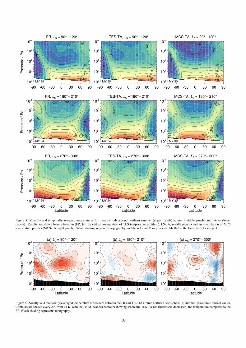
-90 -60 -30 0 30 60 90

103

102

101

100

10-1

Pre

ssure

/ P

a 140

150

150

160

160

170180

190200

210220

FR, LS = 90°− 120°

MY 25

-90 -60 -30 0 30 60 90

103

102

101

100

10-1

140

150

150

160

160

170

180190

200210

220

TES-TA, LS = 90°− 120°

MY 25

-90 -60 -30 0 30 60 90

103

102

101

100

10-1

140

140

150

150

160

160

170180

190200

210220

MCS-TA, LS = 90°− 120°

MY 30

-90 -60 -30 0 30 60 90

103

102

101

100

10-1

Pre

ssu

re /

Pa

140

150

150

160

160

170

170

180

190200

210220

FR, LS = 180°− 210°

MY 24

-90 -60 -30 0 30 60 90

103

102

101

100

10-1

150

150

160

160

160

170180

190

200210

220230

TES-TA, LS = 180°− 210°

MY 24

-90 -60 -30 0 30 60 90

103

102

101

100

10-1

150

150

160

160

160

170

170

170

180

190

200

210

220

MCS-TA, LS = 180°− 210°

MY 30

-90 -60 -30 0 30 60 90Latitude

103

102

101

100

10-1

Pre

ssu

re /

Pa

140

150

150

160

160

170

180190200210

220230240

FR, LS = 270°− 300°

MY 24

-90 -60 -30 0 30 60 90Latitude

103

102

101

100

10-1

140

150

150

160

160

170

180

190

200

210220

230240

TES-TA, LS = 270°− 300°

MY 24

-90 -60 -30 0 30 60 90Latitude

103

102

101

100

10-1

140

150

150

160

160

170

170

180

180

190200

210220

230240

MCS-TA, LS = 270°− 300°

MY 30

Figure 5: Zonally- and temporally-averaged temperatures for three periods around northern summer (upper panels) autumn (middle panels) and winter (lowerpanels). Results are shown from a free-run (FR; left panels) an assimilation of TES temperature profiles (TES-TA; middle panels) and an assimilation of MCStemperature profiles (MCS-TA; right panels). White shading represents topography, and the relevant Mars years are labelled at the lower left of each plot.

-90 -60 -30 0 30 60 90Latitude

103

102

101

100

10-1

Pre

ssure

/ P

a

(a) LS = 90°− 120°

-90 -60 -30 0 30 60 90Latitude

103

102

101

100

10-1

(b) LS = 180°− 210°

-90 -60 -30 0 30 60 90Latitude

103

102

101

100

10-1

(c) LS = 270°− 300°

Figure 6: Zonally- and temporally-averaged temperature differences between the FR and TES-TA around northern hemisphere (a) summer, (b) autumn and (c) winter.Contours are shaded every 2 K from ±1 K, with the (solid, dashed) contours showing where the TES-TA has (increased, decreased) the temperature compared to theFR. Black shading represents topography.

16

0 5 10 15Mass mixing ratio / mg kg-1

103

102

101

100

10-1

Pre

ssure

/ P

a

Initial profile

Iteration 1

Iteration 2

Iteration 3

Figure 1: Example of the scaling process, with the water vapour mixing ra-tio profile scaled each iteration by a factor α (as in Eq. 7) until the column-integrated value agrees with the assimilation. For α > 1 a cutoff is applied at1 Pa, above which no water vapour increase can occur, and points on the profileare not scaled above saturation (dashed line).

0 20 40 60 80Sol

0.0

0.5

1.0

1.5

2.0

Glo

bal sta

ndard

devia

tion / p

r-µ

m

LS = 80°-127°

LS = 174°-235°

LS = 268°-329°

Figure 2: Evolution of σg with time (see Eq. 9) from ensembles of assimila-tions over northern summer (LS = 80◦–127◦), autumn (LS = 174◦–235◦) andwinter (LS = 268◦–329◦). Each ensemble member had different initial con-ditions, obtained by sampling model fields between ±10 sols around the validinitialization time, and then perturbing the initial water vapour fields by ±20%.

0 3 6 9 12 15

Vapour column variance / pr-µm2

(a)

(b)

(c)

Figure 3: Water vapour column variances averaged over the last 10 sols fromensembles of assimilations. Periods are; (a) northern summer, LS = 122◦–127◦,MY 25; (b) northern autumn, LS = 229◦–235◦, MY 24; and (c) northern winter,LS = 323◦–329◦, MY 24. Contours of surface height are plotted to highlight theareas of largest water vapour column variance, which are the Arcadia, Acidaliaand Utopia Planitias, centred at approximately 160◦W, 30◦W and 120◦E.

17

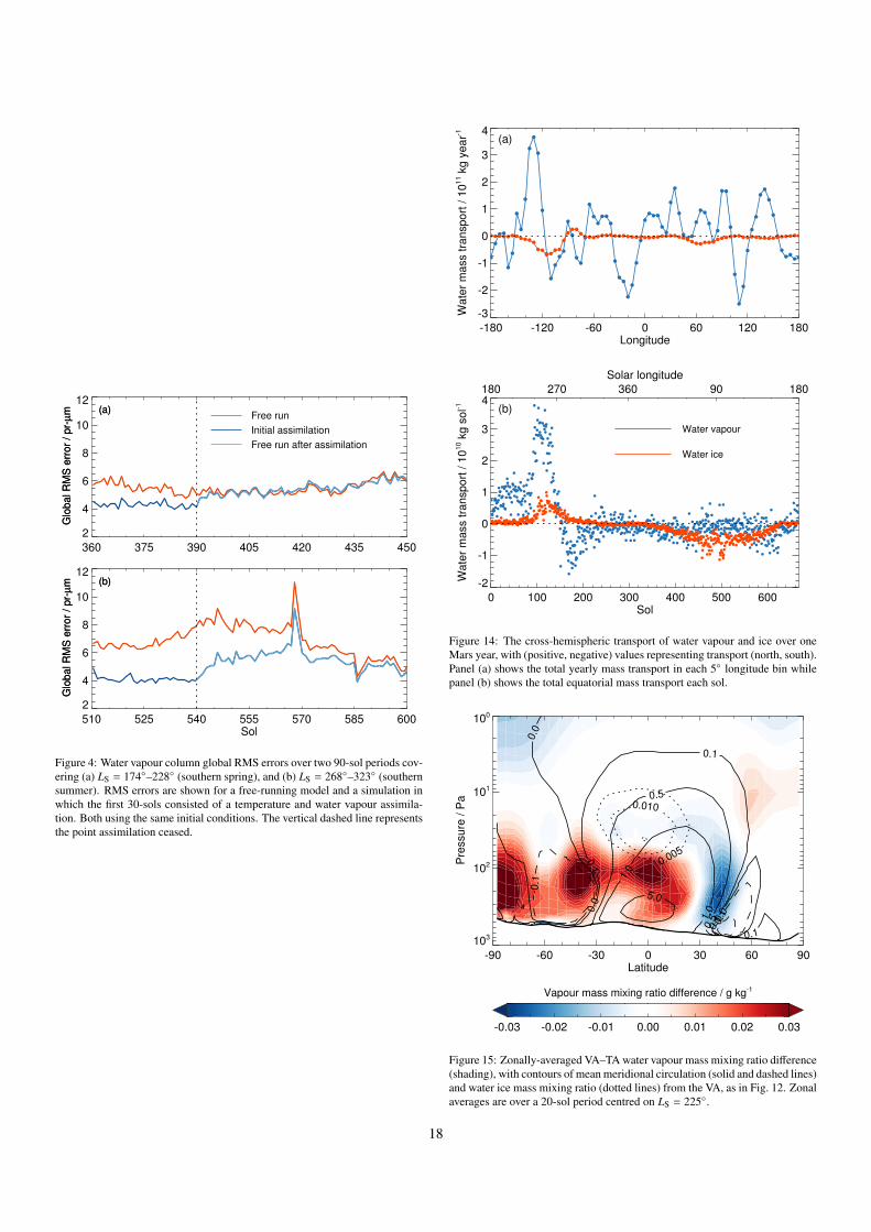
360 375 390 405 420 435 450

2

4

6

8

10

12

Free run

Initial assimilation

Free run after assimilation

Glo

ba

l R

MS

err

or

/ p

r-µ

mG

lob

al R

MS

err

or

/ p

r-µ

m

(a)

(b)

510 525 540 555 570 585 600Sol

2

4

6

8

10

12

Glo

ba

l R

MS

err

or

/ p

r-µ

mG

lob

al R

MS

err

or

/ p

r-µ

m

(a)

(b)

Figure 4: Water vapour column global RMS errors over two 90-sol periods cov-ering (a) LS = 174◦–228◦ (southern spring), and (b) LS = 268◦–323◦ (southernsummer). RMS errors are shown for a free-running model and a simulation inwhich the first 30-sols consisted of a temperature and water vapour assimila-tion. Both using the same initial conditions. The vertical dashed line representsthe point assimilation ceased.

-180 -120 -60 0 60 120 180Longitude

-3

-2

-1

0

1

2

3

4

0 100 200 300 400 500 600Sol

-2

-1

0

1

2

3

4

Water vapour

Water ice

180 270 360 90 180

Solar longitude

(a)

(b)

Wate

r m

ass tra

nsport

/ 1

011 k

g y

ear-1

Wate

r m

ass tra

nsport

/ 1

010 k

g s

ol-1

Figure 14: The cross-hemispheric transport of water vapour and ice over oneMars year, with (positive, negative) values representing transport (north, south).Panel (a) shows the total yearly mass transport in each 5◦ longitude bin whilepanel (b) shows the total equatorial mass transport each sol.

-90 -60 -30 0 30 60 90Latitude

103

102

101

100

Pre

ssure

/ P

a

-0.1

-0.1

0.0

0.0

0.0

0.1

0.1

0.1

0.1

0.5

0.5

1.0

1.0

5.0

0.005

0.010

-0.03 -0.02 -0.01 0.00 0.01 0.02 0.03

Vapour mass mixing ratio difference / g kg-1

Figure 15: Zonally-averaged VA–TA water vapour mass mixing ratio difference(shading), with contours of mean meridional circulation (solid and dashed lines)and water ice mass mixing ratio (dotted lines) from the VA, as in Fig. 12. Zonalaverages are over a 20-sol period centred on LS = 225◦.

18

Simulation No. model levels Data assimilated Vertical extent/resolution of data Mars yearFR 25 None N/A 24/25TES-TA 25 TES temperature profiles ∼40 km / 10 km 24/25MCS-TA 35 MCS temperature profiles ∼85 km / 5 km 30

Table 1: Overview of the simulations performed for the temperature assimilation validation.

Simulation Initial conditions Data assimilatedFR (free run) Model spin-up NoneCR (control run) From assimilation NoneTA (temperature assimilation) From assimilation TES temperature profilesVA (vapour assimilation) From assimilation TES water vapour columns and temperature profiles

Table 2: Overview of the simulations performed for studying the global distribution and transport of water vapour.

180 270 360 90 180Solar longitude

-90

-60

-30

0

30

60

90

Latitu

de

MY24 MY25

0.0

0.5

1.0

1.5

2.0

2.5

3.0

3.5

Num

ber

of observ

ations / 1

03

Figure 7: The number of water vapour column retrievals available for assimilation across each latitude circle, binned by 5◦ in latitude and 2◦ in LS. White areassignify times and locations where there are no data to assimilate.

19

180 270 360 90 180Solar longitude

-90

-60

-30

0

30

60

90

Latitu

de

2

2

2

2

2

2

10 10

10

10

10

10

10

20

20

30

40

0

10

20

30

40

50

Vapour

colu

mn / p

r-µ

m

MY24 MY25

180 270 360 90 180Solar longitude

-90

-60

-30

0

30

60

90

Latitu

de

-5

-5

-5

-5

5

5

5

5

5

5

10

10

15

15

20

-15

-10

-5

0

5

10

15

Vapour

colu

mn d

iffe

rence / p

r-µ

m

180 270 360 90 180Solar longitude

-90

-60

-30

0

30

60

90

Latitu

de

-5

-5

-5-5

5 5

5

5

10

10

15

15

20

(a)

(b)

(c)

Figure 8: Assimilation results over the range LS = 180◦, MY 24 to LS = 180◦, MY 25 showing (a) the zonally-averaged water vapour columns from the VA as afunction of LS and latitude, (b) the VA–TA difference, and (c) the VA–CR difference. The difference plots have shaded contours every 2 pr-µm, with (solid, dashed)lines every 5 pr-µm showing the (positive, negative) differences. The dotted line represents the zero contour. Data are averaged over 2◦ of LS.

20

180 270 360 90 180Solar longitude

0

1

2

3

4

180 270 360 90 180Solar longitude

0

4

8

12

Control run (CR)

Temperature assimilation (TA)

Vapour assimilation (VA)

180 270 360 90 180Solar longitude

-10

-5

0

5

10

MY24 MY25

No

. o

bse

rva

tio

ns /

10

3G

lob

al R

MS

err

or

/ p

r-µ

mG

lob

al m

ea

n e

rro

r /

pr-

µm

(a)

(b)

(c)

Figure 9: (a) The number of water vapour column observations assimilated globally each model time step, with the black line showing the daily average value. (b)Daily average water vapour column global RMS errors. (c) Daily average water vapour column global mean errors. The errors are shown for the CR, TA and VA.The data span the range LS = 180◦, MY 24 to LS = 180◦, MY 25, with the two main gaps centred around LS = 15◦ and 160◦ due to solar conjunction and the MGSspacecraft entering safing mode.

21

180 270 360 90 180Solar longitude

-90

-60

-30

0

30

60

90

La

titu

de

MY24 MY25

(a) TES observations

180 270 360 90 180Solar longitude

-90

-60

-30

0

30

60

90

MY24 MY25

(b) VA results

0.00 0.03 0.06 0.09 0.12 0.15

Ice optical depth / 825 cm-1

Figure 10: Comparison between (a) the absorption-only TES water ice optical depths at 825 cm−1, binned by 5◦ in latitude and 2◦ in LS, and (b) the zonally-averagedwater ice optical depths resulting from the VA, sampled to 2 p.m. local time and averaged over 2◦ of LS (right panel). A mask has been applied to the VA results tomake the comparison clearer.

-180 -120 -60 0 60 120 180

-90

-60

-30

0

30

60

90

La

titu

de

(a) LS = 215°− 235°

-180 -120 -60 0 60 120 180

-90

-60

-30

0

30

60

90

(b) LS = 305°− 325°

-180 -120 -60 0 60 120 180Longitude

-90

-60

-30

0

30

60

90

La

titu

de

(c) LS = 35°− 55°

-180 -120 -60 0 60 120 180Longitude

-90

-60

-30

0

30

60

90

-20

-10

0

10

20

Me

rid

ion

al w

ind

de

via

tio

n /

m s

-1

(d) LS = 125°− 145°

Figure 11: Vertically-averaged meridional wind deviations from the zonal mean between the surface and 100 Pa (∼20 km above the 610 Pa pressure level). Data areaveraged over periods spanning 20◦ of LS, centred on the midpoints of northern hemisphere (a) autumn, (b) winter, (c) spring, and (d) summer.

22

-90 -60 -30 0 30 60 90

103

102

101

100

-90 -60 -30 0 30 60 90

103

102

101

100

Pre

ssure

/ P

a

-90 -60 -30 0 30 60 90

103

102

101

100

0.0

0.0

0.0

0.0

(a) LS = 180°

-90 -60 -30 0 30 60 90

103

102

101

100

-90 -60 -30 0 30 60 90

103

102

101

100

0.0

0.0

0.0

0.0

(b) LS = 225°

-90 -60 -30 0 30 60 90

103

102

101

100

-90 -60 -30 0 30 60 90

103

102

101

100

0.0

0.0

(c) LS = 270°

-90 -60 -30 0 30 60 90

103

102

101

100

-90 -60 -30 0 30 60 90

103

102

101

100

0.0

0.0 0

.0

0.0

(d) LS = 315°

-90 -60 -30 0 30 60 90Latitude

103

102

101

100

Pre

ssure

/ P

a

-90 -60 -30 0 30 60 90

103

102

101

100

0.0

0.0

0.0

(e) LS = 360°

-90 -60 -30 0 30 60 90Latitude

103

102

101

100

-90 -60 -30 0 30 60 90

103

102

101

100

0.0

0.0

(f) LS = 45°

-90 -60 -30 0 30 60 90Latitude

103

102

101

100

-90 -60 -30 0 30 60 90

103

102

101

100

0.0

0.0

(g) LS = 90°

-90 -60 -30 0 30 60 90Latitude

103

102

101

100

-90 -60 -30 0 30 60 90

103

102

101

100

0.0

0.0

0.0

0.0

0.0

(h) LS = 135°

0.00 0.05 0.10 0.15 0.20

Vapour mass mixing ratio / g kg-1

Figure 12: Zonally-averaged water vapour mass mixing ratios from the VA (shaded), with contours of mean meridional circulation (solid and dashed black lines)and ice mass mixing ratio (white lines) overplotted. Each panel shows zonal averages over a 20-sol period centred on the labelled LS values. Panels (a)–(d) arefor MY 24, and panels (e)–(h) for MY 25. The mean meridional circulation contours have pseudo-logarithmic values of [0.1, 0.5, 1, 5]× 109 kg s−1, with (solid,dashed) lines representing (clockwise, anticlockwise) circulation. The ice mass mixing ratio contours denote the values [0.005, 0.01, 0.02, 0.03] g kg−1.

-90 -60 -30 0 30 60 90

-1.0

-0.5

0.0

0.5

1.0(a) LS = 180°

[Qφ]

/ 1

05 k

g s

-1

-90 -60 -30 0 30 60 90

-1.0

0.0

1.0

2.0

3.0

4.0(b) LS = 225°

-90 -60 -30 0 30 60 90

-1.0

0.0

1.0

2.0

3.0

4.0(c) LS = 270°

-90 -60 -30 0 30 60 90

-1.0

-0.5

0.0

0.5

1.0(d) LS = 315°

-90 -60 -30 0 30 60 90Latitude

-1.0

-0.5

0.0

0.5

1.0(e) LS = 360°

[Qφ]

/ 1

05 k

g s

-1

-90 -60 -30 0 30 60 90Latitude

-1.0

-0.5

0.0

0.5

1.0(f) LS = 45°

-90 -60 -30 0 30 60 90Latitude

-1.0

-0.5

0.0

0.5

1.0(g) LS = 90°

-90 -60 -30 0 30 60 90Latitude

-1.0

-0.5

0.0

0.5

1.0(h) LS = 135°

All motions

Mean meridional circulation

Stationary waves

Transient eddies

Figure 13: Vertically-integrated meridional fluxes of water vapour from the VA, with (positive, negative) fluxes representing (northward, southward) transport. Thefluxes have been decomposed into their mean-meridional, stationary wave and transient eddy components, and are averaged over 20 sols centred on the labelled LSvalues. Note the different vertical scale in panels (b) and (c).

23

30 60 90 120 150 180Solar longitude

-90

-60

-30

0

30

60

90

Latitu

de

30 60 90 120 150 180Solar longitude

-90

-60

-30

0

30

60

90

30 60 90 120 150 180Solar longitude

-90

-60

-30

0

30

60

90

0

10

20

30

40

50

Vapour

colu

mn / p

r-µ

m

(a) (b) (c)

Figure 16: Zonally-averaged water vapour columns over the period LS = 30◦–180◦ of MY 25 for (a) the VA, (b) the CR, and (c) the CR with the addition of outlyingwater ice deposits between 120◦–210◦E and 75◦–80◦N. All used the same initial conditions, obtained from the VA.

24