the seasonal variation of interest rates - national bureau of
TRANSCRIPT


52 Essays on Interest Rates
Stable Seasonal Factors
Estimated stable seasonal factors are defined as the mean value ofthe SI ratios for each month. They are called stable or constantbecause they are computed once for the entire sample period. Anydeviation of the SI ratios computed for a given month from thefactor computed for that month is attributed to the irregular com-ponent. In other words, the SI ratios consist of a systematic and arandom component called, respectively, the seasonal and the irregularcomponents. Since the irregular component, expressed as a fractionof the seasonal component, is defined to vary with equal likelihoodabove and below the seasonal component, its ratio to the seasonalcomponent is on average equal to 1. (In the additive case the meanof the irregular component is zero.) Therefore, the mean SI ratio,say for January, is equal to the seasonal component, assumed to bea constant, multiplied by 1. In the absence of seasonality the meanSI ratios would not differ significantly from each other or from 1.
A simple test for the presence of stable seasonality is thereforeto determine the statistical significance of the differences among thecomputed mean SI ratios for each month. The test is a one-wayanalysis of variance of the monthly SI ratios, twelve columns of themfor the twelve months, and the number of rows equalling the numberof annual observations.18 The F-statistic, computed for N full years,is equal to
N times variance of monthly meanstotal variance minus N times variance of monthly means
Except for the graphic method of fitting smooth curves to SIratios of a given month over the years most of the earlier methodsand many of those used currently result in estimates of stable seasonalfactors. For example, the widely used dummy variable technique,whereby the monthly series X is regressed on twelve dummy variables,eleven of which assume the value 1 when the series is measured ina particular month and zero otherwise, the twelfth dummy variablewith the boundaries selected." (Burns and Mitchell, op. cit., p. 49 fn.) Incommenting thus, Burns and Mitchell were concerned with a particular methodof adjustment, the Kuznets amplitude-ratio method (described later); althoughthe principal is apropos of any method.
The X-l I performs the analysis of variance test on the SI ratios after theyhave been modified to reduce the effect of extreme observations. See X-1 1manual, op. cit., p. 5.

Seasonal Variation of Interest Rates 53always assumes the value zero, estimates stable seasonal factors.19 Thecomputation of stable seasonals is justified when there are goodreasons for believing that the parameters are stable in the hypotheticalpopulation from which the observed series is drawn. This belief is notanalogous to the assumed constancy of the parameters in the structuralrelation of, say, consumption and income. A change in the seasonalparameters (as distinct from the estimated factors) of interest ratesdoes not require that the structural relation between, say, interest ratesand money supply change but only that the seasonal pattern of moneysupply change. In fact, by assuming the structural relation fixed, onecan, in principle, estimate it by relating the changes in the seasonalpattern of one series to those in the other.2° Therefore, the assumptionof fixed seasonal parameters for a given series implies the assump-tion of fixed structural relations between this series and others, aswell as of fixed seasonal patterns in these related series.
Moving Seasonal Factors
Typically there are changes not so much in the original cause of theseasonal movement but in the economy's adaptation to it. The in-creased demand for funds in the fall months will result in a seasonalhigh in interest rates only in the absence of a corresponding increasein the supply of funds. The willingness or ability of the bankingsystem to supply the funds will determine whether the increased de-mand will result in higher rates. Seasonal increases in the demand,as well as in the supply, of funds have varied in the postwar period,and the seasonal increase in interest rates has varied along with it.
Changes in seasonal patterns are difficult to distinguish from ir-regular movements—the more difficult, the greater is the varianceof the irregular component relative to that of the total series. Oneidentifies with greater confidence very small changes in the seasonalvariation of money supply, a series with an almost negligible irregular
Michael C. Lovell, "Seasonal Adjustment of Economic Time Series andMultiple Regression Analysis," American Statistical Association Journal, Decem-ber 1963, p. 993.
20 The distinction here is between a structural relation between two economicvariables, on the one hand, and between an economic variable and time, onthe other. Economic models assume constancy in the first case but not thesecond. The fact that a timing relationship has changed does not imply achange in structural relationship since it may reflect merely the timing changeof the variables with which it is structurally related.

54 Essays on Interest Ratescomponent,2' than changes in the seasonal variation of the highlyirregular Treasury bill rate series. The problem of identifying thesechanges is analogous to one of identifying the components themselves:The method already described for that is predicated on the assumedsmoothness of each of the components within its particular frequency;a method for dealing with changes in the components is to assumethese changes themselves evolve along a smooth path. This methodinvolves either fitting by eye a smooth curve to the SI ratios for allthe Januaries, another for the Februaries, and so on, instead of astraight line at the means of the ratios for each month as in thestable factors, or computing a moving average, one month at a time,of the SI ratios adjusted for extreme values. If a simple three-termmoving average were used, for example, the seasonal factor forJanuary 1953 would equal the average of the SI ratios for January1952, 1953, and 1954. In practice, such a simple moving averagewould be used only for series whose irregular component, being small,is in little danger of distorting the evolution of the seasonal factors.A weighted five-term moving average was used to compute the mov-ing seasonal factors of the interest rate series. When the assump-tion of gradually evolving seasonal factors is not apposite, the use ofthis method will impose a spurious similarity on the estimated factorsfor adjacent years of a given month. However, by observing graphsof the SI ratios themselves one may judge the appropriateness of themethod.
There are several alternative methods of caiculating moving seasonalfactors. The simplest one merely divides the whole sample periodinto subperiods and computes stable seasonal factors for each of thesubperiods. This method is particularly useful for separating thesubperiods with clear evidence of seasonality from those without it.There is some evidence, for example, that yields on long-termTreasury securities manifested seasonality during the late fifties butnot before or since. A method based on evolving factors would spreadthe estimated period of seasonality past its true period, at the sametime that it dilutes what seasonality there is. The method is alsouseful when there is an abrupt change in some institutional factoraffecting the seasonal pattern, as, for example, when the Treasury-Federal Reserve accord in 1951 removed the peg on U.S. governmentbonds. Another method is to compute a set of stable factors for thewhole period and, on the assumption that the true factors for any
The variation of the rate of change of the money supply has, of course,a much larger irregular component.

Seasonal Variation of Interest Rates 55
given year remain in fixed relation, compute factors for each yearproportional to the stable factors (that is, with an identical patternbut different amplitude). The proportion used for a given year is theregression coefficient obtained by regressing the SI ratios for that yearon the stable factors, one regression for each year.22 The applicationof this method to the Treasury bill rates would result in an adjustmentnot very different, and perhaps a little better, than that obtained withthe moving average method. This point is considered in the nextsection. Finally, some writers recommend tying the moving seasonalfactors of one series to the variation of related variables. This methodis, of course, limited by the researcher's ability to specify the ap-propriate relations •23
Sometimes the term moving seasonal is applied to a differentphenomenon than the one described above, where the term referredto changes in the true seasonal component requiring an estimationprocedure capable of detecting these changes. If the seasonal com-ponent is a function of the trend cycle component of the same series,then an estimation procedure that assumes the components are in-dependent will yield biased estimates of the moving seasonal factors.The seasonal decline in unemployment, for example, is said to bemilder when the level of unemployment is low than otherwise becausefirms are reluctant to temporarily discharge workers at a time whenthe labor force is fully employed. The appropriate seasonal factorwill therefore vary between periods of high and low unemployment.Unlike the other reason for moving seasonals, this one does notinvolve a change in the relation among the components of the series(sometimes called the structure of the series) but simply a morecomplicated relation among them.
During the four decades preceding the Federal Reserve Act of1913, a problem analogous to that alleged for unemployment pre-vailed on interest rates and the components of the money stock,although with consequences much more severe than the computationof biased estimates of seasonal factors. In his study written for theNational Monetary Commission organized in response to the panicof 1907,24 Kemmerer concluded that the greater incidence of banking
22 See Simon Kuznets, Seasonal Variations in Industry and Trade, New York,NBER, 1933, p. 324.
23 Mendershausen, op. cit., pp. 254—262.24 See also Milton Friedman and Anna Jacobson Schwartz, A Monetary
History of the United States, 1867—1960, Princeton for NBER, 1963, pp.171—172.

56 Essays on Interest Rates
panics in the fall than at other times of the year was due not tothe normal seasonal tightness in the fall money market but to thattightness coming at the same time as a cyclical crisis. The seasonalmovement, in effect, played the role of the proverbial
Even if the seasonal component, expressed as a ratio to the movingaverage, were systematically related to the level of the moving average(or trend-cycle component) the estimated seasonal factors would notreveal this relation. Since the factors are computed from averages ofthe SI ratios across years, the variation of the SI ratios due to thecyclical variation is canceled out in the averaging process. In the caseof an extreme cyclical movement, a related seasonal movement wouldlikely result in an SI ratio that would be regarded as an extreme ob-servation and be eliminated from the computation of the seasonalestimates. However, any relation that exists between the seasonal andcyclical components would present itself in a time series of the SI ratios.Section III considers this point.
Even in the absence of a true relation between the seasonal andcyclical components the inappropriate use of either an additive or multi-plicative adjustment, that is, the use of one when the other is required,will result in an apparent relation between the seasonal and cyclicalcomponents.
When the level of rates is low the basis point equivalent of a multi-plicative adjustment factor is smaller than when the level of rates ishigh. If the true seasonality were additive, and a multiplicative adjust-ment method were used, there would result an inverse relation betweenthe SI ratios and the level of rates. Assume, for example, the true sea-sonal difference for a particular month to be 50 basis points. If inestimating the seasonal variation a multiplicative method were used, theSI ratio computed for this month would be high when the level of rateswere, say, 100 basis points (i.e., 150/100) and low when the levelwere, say, 400 basis points (i.e., 450/400). Application of this test tothe computed SI ratios for the Treasury bill rates does not reveal asystematic inverse relation between these ratios and the level of rates.
28 The evidence on this point is mixed. Kemmerer found that "of the eightpanics which have occurred since 1873 [as of 1910], four occurred in the fallor early winter (i.e., those of 1873, 1890, 1899, and 1907); three broke outin May (i.e., those of 1884, 1893, and 1901); and one (i.e., that of 1903)extended from March until well along in November." After discussing the"minor panics or 'panicky periods,'" he concludes that "The evidence accord-ingly points to a tendency for the panics to occur during the seasons normallycharacterized by a stringent money market." (Op. cit., p. .232.)

Seasonal Variation of Interest Rates 57
However, the opposite procedure designed to test the efficacy of a multi-plicative adjustment, assuming the true seasonal were multiplicativeand the estimates additive, fails to confirm the appropriateness of amultiplicative adjustment. The question is therefore open and invitesdeference to convention—which is to use a multiplicative adjustmentunless an additive one is clearly indicated.26
There is a method that combines elements of both the additive andmultiplicative adjustment. Seasonal-irregular ratios are computed foreach month and the set for each month regressed on the trend-cyclecomponent for that month; twelve regressions in all. The constant termof each regression is an estimate of the additive component of thatmonth's seasonal factor and the regression coefficient of the multipli-cative component. This method, however, assumes stable seasonality inthe sense used earlier in this report.27
Seasonal Adjustment on Computers
The X-1 1 program, used in this study, embodies a series of refine-ments in the original ratio-to-moving-average technique that Macaulaydeveloped in the 1930's. By reducing the cost and virtually eliminatingthe tedium of the vast number of elementary calculations this methodof adjustment requires, the program makes feasible the use of complexweighting schemes in computing moving averages that are both elastic(i.e., remain faithful to the original series) and smooth (i.e., avoidthe irregular wiggles). It allows, moreover, the extensive use of itera-tion to mitigate the obscuring influence of the irregular component onthe separation of the seasonal from the trend-cycle components. Itsmost important advantage is the reduction in the time-cost and skillsrequired in manual adjustments.
26 See Julius Shiskin and Harry Eisenpress, Seasonal Adjustment by ElectronicComputer Methods, Technical Paper 12, New York, NBER, 1958, p. 434.
27 There is clearly room here for variations on a theme. One can adapt theregression method to allow for a moving seasonal by applying the regressionmethod as stated and applying the X-l 1 method to the residuals of theregressions. In that case one could obtain: an additive component, a componentrelated to the trend cycle, and a moving seasonal component. Since this studyuncovered no evidence of a relation between the seasonal and trend-cyclecomponents of the interest rate series there was no reason to experiment withthis method. In his exhaustive article, Mendershausen (op. cii.) describes manyexotic techniques for circumventing this or that problem of conventionalmethods; virtually all of them are in desuetude either because they introducedother problems or they were too unwieldy.

58 Essays on Interest Rates
The program's advantages are particularly obvious through the stagein which the modified seasonal-irregular ratios or differences are com-puted as, of course, are their mean values, or the stable seasonal factors,when relevant. An experienced draftsman, however, can graphically fitmoving seasonals to. the SI ratios as well as the program does, andprobably better than the program does when the series has a prominentirregular component. Moreover, judgment is often required in deter-mining whether an adjustment for any subperiod should be undertakenat all. Since the analysis of variance is a test of the means of the SIratios for the whole sample period, there is some danger that the pres-ence of a relatively strong seasonal component in one subperiod willaffect the means for the whole period sufficiently to lend an apparentsignificance to the computed differences among them. (This effect wouldhave to be large enough to overcome the increased within-group vari-ance as a result of the greater heterogeneity of the SI ratios of a givenmonth that a moving seasonal implies.) The program adjusts the wholeseries regardless of the results of the analysis of variance. The usercannot rely on the F-test alone to decide whether to accept the adjust-ment in its entirety.
The absence of objective criteria for selecting the period of adjust-ment, the extent of the adjustment, or the quality of the results28 pre-cludes an elaborate tabulation of this study's findings replete with stan-dard errors. Nevertheless, from the descriptive statistics, the diagrams,and the verbal entourage, patterns emerge that are worth noting. SectionIII presents this material for seventeen interest rate series.
III. THE EVIDENCE OF SEASONALITYIN INTEREST RATES
This section evaluates the evidence of seasonality in postwar interestrates and suggests suitable adjustments where appropriate. The evalua-tion consists of graphically identifying biases in the SI ratios over orunder the 100.0 level. While the one-way analysis of variance test forseasonality is a useful method for identifying systematic deviations ofthe SI ratios from 100.0, its reference to the entire period makes itineffective as a means of distinguishing the s.ubperiods with evidence of
26 "A statistician who has struggled with seasonal adjustments of numeroustime series is not likely to underestimate the part played by 'hunch' and'judgment' in his operations." (Burns and Mitchell, op. cit., p. 44.)

Seasonal Variation of Interest Rates 59
seasonality from those without it.2° The consistent deviation of a givenmonth's SI ratio in the same direction from the 100.0 line is strongevidence of seasonality regardless of the variation in the magnitude ofthese deviations, that is, in the seasonal amplitude. The evidence ofseasonality is weak when there are constant reversals of direction orwhen the relationship among the patterns of SI ratios is generally un-stable from year to year. The summary statistics that most computerprograms for seasonal adjustment supply (such as the average month-to-month change in the seasonal component by itself or relative to thatof the other components) do not help evaluate the evidence of season-ality since, aside from the analysis of variance test, they only sum-marize what the program has done. They do not provide independentmeasures of either the evidence of seasonality or the quality of the ad-justment. Once the existence of a seasonal pattern is confirmed and theadjustment decided, then the summary statistics provide a useful sum-mary of the results.
In seasonal analysis, as in regression analysis, one places greaterconfidence in tests for the existence of a relation than in its actualmeasurement. In addition to the problem of sampling error commonto both analyses, the moving seasonal amplitude implies changingparameters and requires the adjustment method, in effect, to shoot ata moving target. Except for a few experiments this study does notoriginate any methods of adjustment, nor does it even compare theadjustments obtainable with existing methods.3° Instead, charts of theseasonal factors obtained with the X-1 1 are superimposed on chartsof the corresponding SI ratios to determine the method's success incapturing what appears to be the systematic movement of the SI ratios.There is no question but that one could fit by eye a curve that is morefaithful than is the curve of factors to variation of the SI ratios; in theextreme, one could perfectly fit a curve to the SI ratios by simplyconnecting the points—that is, by simply treating them as the factors.The art of the adjustment is in identifying the systematic movementof the SI ratios. When the pattern of SI ratios is stable from year toyear there is no problem; nor is there any when the seasonal amplitudechanges gradually or the pattern evolves with an apparent method. Butduring transition periods, in which the series has strong irregular move-
20 One can apply the analysis of variance to separate subperiods, but theproblem of choosing the limits of the subperiods remains.
The potential gain from these experiments is not, in this study's view,commensurate with the effort required.
60 Essays on interest Rates
ments, such as 1954, the SI ratios and estimated factors appear to bevirtually unrelated. This study recommends ignoring the adjustmentwhen the gap between the two is pervasive.
Short-Term Securities
Summary Statisfics
Table 2-1 lists some of the summary statistics that are useful in de-scribing the extent and significance of seasonal influence.31 Columns1—3 divide the total variance of the series into the parts due to eachof the three components: the trend-cycle, seasonal, and irregular. Thesefigures are analogous to readings from the spectral density function,which decomposes the variance of a time series according to the fre-quency of the recurring variation.82 Column 4 lists the average month-to-month percentage changes (without regard to sign) of the seasonalcomponent, and column 5 the ratio of column 4 to the correspondingstatistics of the cyclical component. These figures, columns 1 through 5,strike averages for the whole study period, averages not of the trueseasonal but of the estimated one, including a spill-over into periodswithout significant seasonality. Columns 7—10 give the dates and am-plitudes of the highest and lowest seasonal factors observed during thestudy period.
But these figures may be only statistical artifacts; hence, the needexists to ascertain their statistical significance. To partially satisfy thisneed, column 6 records the F statistics.
The F statistic may be low for any of several reasons, the enumera-lion of which will help in evaluating the charts that follow. The most
The statistics are copied directly from the X-1 I printout and are describedmore fully in the X-11 Manual, op. cit.
32 Some recent studies have applied spectral analysis to the problem ofidentifying seasonal variation. While the principle is the same as that in themoving average method—to simultaneously or sequentially filter, or separate,different frequencies of variation—spectral analysis is a more sophisticatedand more rigorous method of doing so. Some of the mathematical advantageis lost, however, in its application to a limited number of observations. Thismethod, moreover, provides no direct adjustment for the seasonal and resembles,in this respect, analysis of variance instead of regression analysis. In Chapter 7of this book, Tom Sargent has applied spectral analysis to interest rates, amongother financial variables, and has reached conclusions virtually identical to thosein the present study with respect to the extent and evolution of the seasonalin interest rates.

TAB
LE 2
-1. M
easu
res o
f the
Rel
ativ
e Im
porta
nce
of th
e Se
ason
al C
ompo
nent
s of t
he F
our S
erie
s of S
hort-
Term
Secu
ritie
s, 19
48—
65
Ave
rage
Rat
io o
fM
onth
-to-M
onth
Col
umn
4D
ate
and
Fact
or o
f Sea
sona
l Hig
h
.
Ser
ies
Perc
enta
ge o
fTo
tal V
aria
nce
ofSe
ries D
ue to
Each
Com
pone
nt
IC
S(1
)(2
)(3
)
Perc
enta
geC
hang
esW
ithou
t Reg
ard
to S
ign
ofSe
ason
alC
ompo
nent
3 (4)
to C
orre
-sp
ondi
ngFi
gure
sfo
r the
Cyc
lical
Com
pone
ntS/
C(5
)
F Te
st fo
rSt
able
Seas
onal
itya
(6)
and
Low
for W
hole
Per
iodb
Hig
hLo
w
Fact
or(p
erce
nt-
Dat
eag
e)D
ate
(7)
(8)
(9)
Fac
tor
(per
cent
-ag
e)(1
0)
Yie
lds o
n:91
-day
bill
s37
.72
42.5
219
.76
2.54
0.68
9.66
2D
ec. 1
957
113.
9Ju
ly 1
957
87.4
9—12
mon
thse
curit
ies
35.9
149
.77
14.3
21.
850.
544.
557
Dec
. 195
610
9.0
June
195
790
.7C
omm
erci
alpa
perc
35.3
842
.98
21.6
41.
81.7
14.
034
Dec
. 195
810
7.5
May
195
992
.8B
anke
rs'
acce
pt-
ance
s24
.57
49.3
926
.04
2.07
.72
11.2
93D
ec. 1
957
111.
4Ju
ly 1
956
89.3
aAll
ratio
s are
stat
istic
ally
sign
ifica
nt a
t the
5 p
er c
ent l
evel
.bA
mov
ing
seas
onal
com
pone
nt w
as e
stim
ated
for b
oth
serie
s. C
olum
ns 7
and
9 li
st th
e da
tes w
hen
the
ampl
itude
s of t
he se
ason
alva
riatio
ns w
ere
grea
test
and
col
umns
8 a
nd 1
0 th
e va
lues
of t
he e
stim
ated
seas
onal
fact
ors f
or th
ese
date
s.C
The
sam
ple
perio
d fo
r com
mer
cial
pap
er ra
tes e
nds i
n Ju
ne 1
965.

62 Essays on interest Ratesimportant reason, of course, is the absence of any bias in the monthlySI ratios away from the mean value of 100.0; in other words, no sea-sonality. But a low F statistic does not imply the absence of seasonalityover the whole sample period. The smaller the subperiod of true sea-sonality the greater the burden on this period's SI ratios to influence themeans for the whole sample period and thereby enlarge the betweenmeans variance, the numerator of the F ratio. The burden is aggravatedby the fact that a moving seasonal component combines with the ir-regular component to enlarge the within-group variance, the denomina-tor of the F ratio. When, for example, the F statistic is computed forlong-term Treasury securities over the entire period, its value (1.787)signifies the absence of seasonality; whereas, when computed overthe period. 1955 through 1962 the result (4.726) confirms the pres-ence of seasonality. Similarly, the F statistic in Table 2-1 for nine-to twelve-month Treasury securities is low because the seasonal pat-tern before 1955 was at best highly irregular. When the seasonalpattern changes over the sample period, even when in each subperiodthe pattern is unambiguous, the F statistic suffers as the differencesamong the mean monthly SI ratios are reduced. Combine this prob-lem with the fact that seasonal patterns do not change instantaneouslybut rather evolve through periods of transition during which a coherentpattern is virtually nonexistent. In the eighteen-year sample periodthe seasonal pattern of commercial paper rates underwent severalchanges, and the low F statistic shown in Table 2-1 in part reflectsthis fact.33 Finally, the F statistic may be low not because there isno seasonality but because of a strong irregular component; the meansof the SI ratios are different from 100.0, but the standard errors ofthe means are high. This condition applies to all the interest rateseries and in particular to commercial paper rates and yields onmunicipal bonds. Here again the diagrams are essential for deter-mining whether the seasonal pattern has sufficient stability to war-rant adjustment.
At its highest the seasonal component pushes the Treasury bill rate14 per cent (rounded to nearest integer) above its trend-cycle value;at its lowest, 13 per cent below. For a bill rate in the neighborhoodof 4 per cent (i.e., 400 basis points) these seasonal factors correspondto about 50 basis points.34 At 11 per cent on either side of the trend-
These changes are described later in the section.These figures are actually underestimates since they embody the dampening
effects of the lower peak levels of adjacent years. Later in this section anexperiment is described that exemplifies this point.

Seasonal Variation of Interest Rates 63
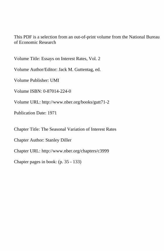
cycle values, the peak seasonal amplitude for yields on bankers' ac-ceptances is somewhat less. Relative to the total variation of theseries, however, the seasonal component of the yields on bankers' ac-ceptances is the most important of the four series, and its F statisticis highest. The diagrams, to be. discussed presently, support the con-clusion that this series evinces the strongest seasonal component. Theseries for which the summary statistics are least reliable is the serieson commercial paper rates, for which, in addition, the F statistic islowest. The diagrams will justify this conclusion as well.
Treasury Bill Rates
Chart 2-7 plots the seasonal factors for Treasury bill rates super-imposed on the corresponding SI ratios. From a relative high inJanuary the Treasury bill rate seasonal pattern typically declines pastseasonally neutral February, downward through the spring monthsto its trough in June or July and then turns sharply upward throughseasonally neutral August to September, from which it rises graduallyto its peak in December.35 Surprisingly, this pattern is quite apparent,although the amplitude is small, in 1948, when the Federal Reservepegged the prices of Treasury bills within narrow limits. This curveis shown in the first panel of Chart 2-7 together with the unmodifiedSI ratios. In subsequent panels of Chart 2-7, the pattern is shown todissolve until about 1953 and then gradually to emerge again, butwith greater amplitude, in the middle fifties, keeping this shape intothe sixties as its amplitude virtually disappeared. By 1965 there waslittle left but a 2 per cent trough in June—July and a 2 per cent peakin December—January.
The factor curves, the broken lines of Chart 2-7, are for the mostpart dampened versions of the corresponding SI ratios, although attimes the factor curve for one year betrays the influence of itspredecessor more than that of its contemporary SI ratios. In thisregard the factor curves ignore certain abrupt movements of the SIratios, as in April 1955, the program being designed to sidesteppoints it regards as extreme.3°
Before 1957, the movement between September and December was notmonotonic.
Briefly, an extreme point is one that falls outside the range of 1.5 standarddeviations, the latter computed for the entire set of data several times toeliminate the effect on it of the extreme points. The extremes are weighted

64 Essays on Interest RatesC}IART 2—7. SI Ratios and Seasonal Factors for Treasury Bill Rates,1948—65
FMAMJ JASON FMAMJ J A
SI ratiosSeasonal factors
Index Index Index

Seasonal Variation of interest Rates 65
The relative stability of the seasonal pattern is in part a measureof the adjustment's effectiveness since the program does not attemptto directly fit the solid lines in Chart 2-7. Instead it smooths the SIratios month by month as shown in Chart 2-8. As a given month'sCHART 2—8. Variation of Monthly Factor Curves and SI Ratios ofTreasury Bill Rates, 1948—65
SI rQtiosSeasonal factors
factors evolve through the years, any persistent change in their rela-tion to another month's factors, that is, any change in the orderinglinearly from 1 to 0 as they fall between 1.5 and 2.5 standard deviations. Anextreme SI ratio different from 100 by two standard deviations is weighted 0.5.See X-11 Manual, op. cii., pp. 4—5.

66 Essays on Interesr Rates
of the twelve factors, will change the seasonal patterns given inChart 2-7. Barring the extremes, the factor curves in Chart 2-8 fit theSI ratios quite closely although severely dampening their movement.One may wish to quarrel with the fit at a few places, but it will soonbe shown that any reasonable alterations would have little quantitativeimportance. The two or three years preceding 1954 and following1960 appear overly dependent on the years in between; and cor-respondingly, the peak period is excessively dampened. Aside fromthe transitional months, February and August, the monthly factorcurves trace out the bell-shaped curves noted earlier, inverted in thelow months, of course, and most of them remain above 100 or below100 throughout the period. While most of the curves as of 1965roughly coincide with the 100.0 line, the curves for July and Decem-ber are still about 2 per cent under and over the line, denoting thepersistence of a small seasonal variation in Treasury bill rates.However, the pattern for the last four years differs somewhat fromthat in earlier years: the trough appears in June instead of July; theJanuary factors become at least as prominent as the ones for Decem-ber; and, in the last two years, the November factors dip below the100.0 line. Similar changes will be shown to have occurred in yieldson bankers' acceptances as well.37
Other Short-Term Rates
The seasonal patterns of the other short-term rates considered, ex-cept for commercial paper rates prior to 1956, are very similar tothe one for Treasury bill rates. The similarity is greatest in the peakperiod, when the patterns for all the series have their greatest stability.Table 2-2 lists the simple correlation coefficients between the twelveseasonal factors for Treasury bill rates and those for the other seriesover selected years. In 1957 the correlations were all in excess of .95,indicating virtual identity among the four patterns; by 1965, however,the correlations were much less, and could be in part the spuriousaftermath of the earlier similarity.
Closest in pattern and evolution to that of Treasury bill rates isthe seasonal movement of yields on bankers' acceptances. As in thecase of bills, the seasonal pattern for yields on bankers' acceptances
The appendix to this section uses alternate adjustment procedures toevaluate the X-I 1 adjustment of Treasury bill rates.
'1

Seasonal Variation of Interest Rates 67TABLE 2-2. Simple Correlation Coefficients Between the Seasonal Factorsfor Treasury Bill Rates and Those for Other Short-Term Rates for SelectedYears
1953(1)
1957(2)
1963(3)
1965(4)
Bankers' acceptances .6430 .9742 .7926 .5283Commercial paper .1380 .9724 .8917 NA9—12 month Treasury securities .8447 .9510 .7700 .6492
NOTE: The numbers are all simple correlation coefficients between the seasonalfactors of Treasury bill rates and the factors in the corresponding years for the otherthree series.
NA = not available.
is fairly stable from 1948 through 1950, but, again like bills, the fitis less adequate from 1951 through 1954. In Chart 2-9 the estimatedfactors are shown to grossly exaggerate the trough in July. Sea-sonality exists in the period (July, for example, is always below the100.0 line and December above), but its pattern is less stable thanand differs from the patterns of other years. During the peak periodits pattern is the familiar high in January, declining past neutral Febru-ary through the spring lows to a trough in July, then climbing steeplyupward to September and, more gradually, to a December peak. Al-though its peak amplitude, at 12 per cent on either side of the corre-sponding trend-cycle values, is somewhat less than the peak in thebill rate seasonal pattern, the seasonal amplitude on yields on bankers'acceptances is more prominent in the total variation of the series(columns 3 and 5 of Table 2-1), and the estimated factors are morefaithful to the SI ratios (Chart 2-9). Beginning in 1959. the patternbegins to change somewhat, the trough shifts from July to June andthe peak from December to January. These changes, as well as thedip in November, are virtually identical to those that occurred some-what later in Treasury bill rates. Chart 2-9 reveals the low and de-clining seasonal amplitude in yields on bankers' acceptances in thesixties. Although the last year of the adjustment period, is alwaystricky, the factors for 1965 appear to signal the end of the seasonalcomponent.
Because its pattern is less stable than the patterns of the two short-term series described above, the seasonal variation of commercialpaper rates is more difficult to isolate. Chart 2-10 plots the SI ratiosand corresponding factors for commercial paper rates. From 1948

68 Essays on Interest RatesCHART 2—9. SI Ratios and Seasonal Factors for Bankers' AcceptanceRates, 1948—65
Index110
SI rotLosSeasonal factors
Index Index
90 -1949
-
110
100
- -
II,...,
90
1950
90 - - 110
110
100
1951
.',._
- -
100
901952
——
90
110
100
90
110
100
- - 110
90
110
100
90
-
1954
-
1956
90 -
I I I II I I I I I
F MAM J .J A SO ND
Index
110

Seasonal Variation of Interest Rates 69CHART 2—10. SI Ratios and Seasonal Factors for Commercial PaperRates, 1948—65
J FM AM J JASON 0
Index
90
110
100
90
110
100
90
110
100
90
Index
SI rattosSeasonal factors
Index Index130
10
100

70 Essays on Interest Rates
through 1950 the seasonal pattern, except for a high in October, isvirtually the mirror image of the pattern in the late fifties—the firsthalf year in the earlier period being above the 100.0 line, the secondhalf below. The pattern evolves through a transition period in 1951to a pattern that extends through 1955 and is quite similar to the onefor long-term rates. Beginning with a low in January the factors dropto a trough in March, turn up through May or June to a peak inOctober and then sharply down. The pattern in 1955 already blendsinto the new pattern that is characteristic of the other short-termseries: From a high in January the factors turn down through neutralFebruary and the springtime lows to a trough in July then go upthrough neutral August to a peak in December. This pattern persiststhroughout the period of peak seasonality in the late fifties, duringwhich, however, the seasonal amplitude never exceeds 8 per cent ofthe corresponding average values of the series. Beginning in 1962 thepattern appears to drift back towards the earlier one that resembledthe pattern of long-term series. Nevertheless, the seasonal amplitudepersists through the end of the period.
As in the case of the other short-term series, there is a repetitiveripple in the yields on nine- to twelve-month Treasury securities from1948 through 1950, but, as Chart 2-11 shows, the factors do not fitthe SI ratios as well as in the case of the other short-term series.Several years of erratic movement follow before the final patternemerges in 1955. Choppy at first, it evolves rapidly into full shapein 1957 and slowly down again but persisting through the end of theperiod. Indeed, in 1965 the amplitude is greater and the pattern morediscernible than in the case of bill rates.
The pattern during the late fifties is very similar to that of the othershort-term series except that the trough comes a month earlier (inJune) and a fall plateau replaces the December peak. This change inpattern is in the direction of the long-term series.
Summary of Short-Term Series
While the seasonal patterns of short-term rates are not entirely uni-form throughout the postwar period, for the most part they have incommon springtime lows and a midyear trough, as well as fall highsand a December peak continuing with some diminution through Jan-uary. This pattern describes all four series in the period of greatestseasonality, 1956 through 1960. Treasury bill rates and yields on

Seasonal Variation of Interest Rates 71
CHART 2—11. SI Ratios and Seasonal Factors for Yields on Nine. toTwelve-Month U .S. Government Securities, 1948—65
SI rutLosSeasonal factors
Index Index Index Index1 130
72 Essays on Interest Ratesbankers' acceptances sustain this pattern throughout the 1948—65period, although not with as much stability and amplitude as duringthe 1956—60 period. The patterns for commercial paper rates prior to1956 are quite different from those of the other short-term rates and,in fact, resemble those of the long-term rates that are described be-low. There are actually two distinct patterns for commercial paperrates during 1948—55, a fact making the adjustment for this periodof questionable value. While the pattern for to twelve-monthTreasury securities prior to 1955 is quite similar to the one for Trea-sury bills (column 1 of Table 2-2), the factors are not sufficiently faith-ful to the SI ratios, in this study's view, to warrant an adjustment. Inthe later period, however, the seasonal influence is unambiguous;Chart 2-12 plots the time series of seasonal factors of the four short-term series considered in this study.
After 1960 the seasonal amplitudes of all the short-term seriesrapidly decline. While some seasonality persists after 1963, an adjust-ment will unavoidably introduce some additional error into the series.Whether the elimination of the true seasonal is worth the increaseddanger of introducing error as a result of adjusting for a spuriousseasonal factor is an isssue the user must decide. Table 2-3 lists theperiods during which, in this study's view, the seasonal is worth ad-justing for.
TABLE 2-3. Suggested Periods for Adjusting Short-Tenn Series
Security Adjustment Period
Treasury bill rates 1948—65Bankers' acceptance rates 1948—63Commercial paper rates 1956—659—12 month Treasury security rates 1955—65
Long-Term SecuritiesSummary Statistics
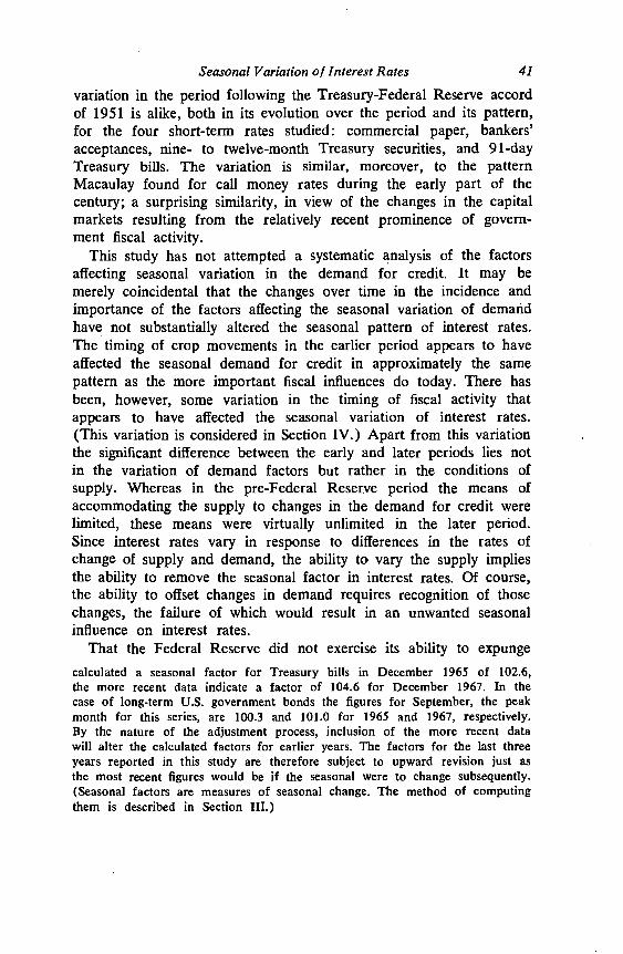
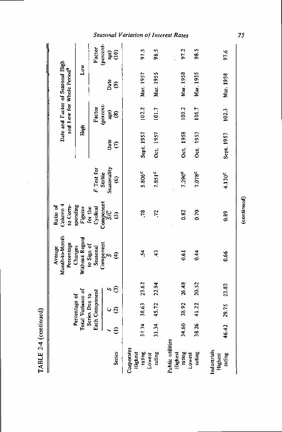
The seasonal amplitudes of yields on long-term bonds are not high.In only two of the thirteen cases listed in Table 2-4 does the highestestimated factor for a given bond exceed 4 per cent and in only fourcases 3 per cent (column 8). Notwithstanding the low amplitudes,the computed F statistics signify stable seasonality in all but twocases and in most cases by a wide margin (column 6). Finally,

CH
AR
T 2—
12. S
easo
nal F
acto
rs fo
r Sho
rt-Te
rm In
tere
st S
erie
s, 19
48—
65In
dex
Inde
xI
II
II
II
II
II
II
II
I
—B
anke
rs a
ccep
tanc
e ra
tes
110-
Co
alat
—
110
100 90
-U
. S. G
ovt.
secu
ritie
s, 9
—12
mon
ths
120
— -C
90 120 10
—T
reas
ury
bill
rate
s
II
II
—1
1948
'51
'53
'55
'57
'59
'61
'63
'65
90
II
II
II
II
I80

TAB
LE 2
-4. M
easu
res o
f the
Rel
ativ
e Im
porta
nce
of th
e Se
ason
al C
ompo
nent
s in
the
Var
iatio
n of
Yie
lds o
n Lo
ng-T
erm
Bon
ds, 1
948
—65
Ave
rage
Rat
io o
fM
onth
-to-M
onth
Col
umn
4D
ate
and
Fact
or o
f Sea
sona
l Hig
h
Perc
enta
ge o
fTo
tal V
aria
nce
ofSe
ries D
ue to
Each
Com
pone
nt
Perc
enta
geC
hang
esW
ithou
t Reg
ard
to S
ign
ofSe
ason
al
to C
one-
spon
ding
Figu
res
for t
heC
yclic
alF
Test
for
and
Low
for W
hole
Per
ioda
Hig
hLo
w
Fact
orFa
ctor
IC
SC
ompo
nent
SC
ompo
nent
S/C
Stab
leSe
ason
ality
(per
cent
-(p
erce
nt-
Dat
eag
e)D
ate
age)
Serie
s(1
)(2
)(3
)(4
)(5
)(6
)(7
)(8
)(9
)(1
0)
Mun
icip
alsb
Hig
hest
ratin
g44
.23
34.7
821
.00
1.18
0.78
Sept
. 195
810
4.7
Feb.
195
896
.6Lo
wes
tra
ting
45.9
736
.30
17.7
20.
860.
701.
515
Sept
. 195
810
2.3
Apr
. 196
097
.7H
igh
grad
e(S
& P
)55
.38
26.7
417
.88
1.05
0.82
Sept
. 195
810
3.5
Feb.
195
507
.1
Rai
lroad
sH
ighe
stra
ting
34.6
545
.46
19.8
90.
440.
667•
230C
Sept
. 195
710
1.8
Mar
. 195
798
.3Lo
wes
tra
ting
36.9
238
.36
24.7
10.
590.
81'L
lllc
Dec
. 195
610
1.6
Mar
. 195
497
.9
(con
tinue
d)
TAB
LE 2
-4 (c
ontin
ued)
0 0 0 0
Ave
rage
Rat
io o
fM
onth
-to-M
onth
Col
umn
4D
ate
and
Fact
or o
f Sea
sona
l Hig
h
Perc
enta
ge o
fTo
tal V
aria
nce
ofSe
ries D
ue to
Each
Com
pone
nt
Perc
enta
geC
hang
esW
ithou
t Reg
ard
to S
ign
ofSe
ason
al
to C
orre
-sp
ondi
ngFi
gure
sfo
r the
Cyc
lical
F Te
st fo
r
and
Low
for W
hole
Pen
oda
Hig
hLo
w
Fact
orFa
ctor
IC
SC
ompo
nent
SC
ompo
nent
S/C
Stab
leSe
ason
ality
(per
cent
-(p
erce
nt-
Dat
eag
e)D
ate
age)
Ser
ies
(1)
(2)
(3)
(4)
(5)
(6)
(7)
(8)
(9)
(10)
Cor
pora
tes
Hig
hest
ratin
g37
.74
38.6
323
.62
.54
.78
5•80
6CSe
pt. 1
957
102.
2M
ar. 1
957
97_s
Low
est
ratin
g31
.34
45.7
222
.94
.43
.72
7•85
1CO
ct.
1957
101.
7M
ar. 1
955
98.5
Publ
ic u
tiliti
es.
Hig
hest
ratin
g34
.60
38.9
226
.48
0.61
0.82
Oct
. 195
810
3.2
Mar
. 195
897
.2Lo
wes
tra
ting
38.2
641
.22
20.5
20.
440.
70O
ct. 1
957
101.
7M
ar. 1
955
98.5
Indu
stria
lsH
ighe
stra
ting
46.4
229
.75
23.8
30.
660.
894j
30C
Sept
. 195
710
2.3
Mar
. 195
897
.6
(con
tinue
d)

TAB
LE 2
-4(c
oncl
uded
)
Ave
rage
Rat
io o
fM
onth
-to-M
onth
Col
umn
4D
ate
and
Fact
or o
f Sea
sona
l Hig
h
Perc
enta
ge o
fTo
tal V
aria
nce
ofSe
ries D
ue to
Each
Com
pone
nt
Perc
enta
geC
hang
esW
ithou
t Reg
ard
to S
ign
ofSe
ason
al
to C
one-
spon
ding
Figu
res
for t
heC
yclic
alF
Test
for
and
Low
for W
hole
Per
ioda
Hig
hLo
w
Fact
orFa
ctor
IC
SC
ompo
nent
SC
ompo
nent
S/C
Stab
leSe
ason
ality
(per
cent
-(p
erce
nt-
Dat
eag
e)D
ate
age)
Ser
ies
(1)
(2)
(3)
(4)
(5)
(6)
(7)
(8)
(9)
(10)
Indu
stria
lsLo
wes
tra
ting
29.1
253
.34
17.5
40.
360.
57O
ct.
1957
101.
4M
ar. 1
958
98.6
U.S
. Tre
asur
yLo
ng te
rm7.
5140
.42
2.08
0.50
0.55
1.78
7Se
pt. 1
957b
102.
8A
pr. 1
957
98.0
3—5
year
s3.
7337
.76
8.51
1.45
0.71
Sept
. 195
710
5.8
Apr
. 195
995
.2
aA m
ovin
g se
ason
al c
ompo
nent
was
est
imat
ed fo
r the
four
serie
s. C
olum
ns 7
and
9 li
st th
e da
tes w
hen
the
ampl
itude
s of t
hese
ason
al c
ompo
nent
wer
e gr
eate
st a
nd c
olum
ns 8
and
10
the
valu
es o
f the
est
imat
ed se
ason
al fa
ctor
s for
thes
e da
tes.
bThe
est
imat
ed se
ason
al fa
ctor
for S
epte
mbe
r 195
8 w
as a
lso
102.
8.cs
igni
fican
t at t
he 1
per
cen
t lev
el.
I

Seasonal Variation of Interest Rates 77
again notwithstanding the low peak amplitudes, as well as the sea-sonal components' relatively low average month-to-month percentagechanges without regard to sign (column 4), the estimated percent-ages of total variation of the series due to the seasonal components(column 3) are roughly comparable and a little higher than thecorresponding figure for Treasury bill rates.
These summary statistics are likely to be more reliable than thecorresponding statistics for short-term securities because in the long-term bond rates, exclusive of the two Treasury series, the seasonalitypersisted throughout most of the study period, although with somechanges in both pattern and amplitude. The summary statistics forthree- to five-year and long-term Treasury securities, however, largelyreflect the seasonal flourish in the. late fifties. Both its small amplitudeand its shifting pattern likely contribute to the persistence of sea-sonality in long-term bonds (as of 1965 the seasonal influence inmost of the series was minute but discernible) since these character-istics in effect obscure the seasonal variation and thereby lessen thelikelihood of investors trading them away.38
Although there is a general bell-shaped pattern to the seasonalamplitudes of the long-term securities during the postwar period, therelative rise in the late fifties is not as pronounced as in the case ofthe short-term securities nor is it as pronounced in the private long-term rates as in the Treasury rates. Table 2-5 lists the variances ofthe seasonal factors of a given year for selected years for all thesecurities considered in this study. The variance of the twelve monthlyfactors is a convenient measure of the over-all seasonal amplitudefor a given year. The bell-shaped pattern refers to the increase inthe securities from 1953 to 1957 and their decrease to 1963. (Thebell is actually quite symmetrical, a fact that is hidden by the differ-ent spans of the two periods.) Except for the railroad (lowest quality)securities, the table supports the generalization stated above.
There is a curious consistency in the relations among the seasonalfactors of the several long-term series, a consistency for which thereis no mechanical explanation. In Table 2-5, for example, the seasonal
88 A small amplitude does not by itself impugn the significance of theseasonal component. The seasonal amplitude for the series on the stock ofmoney, for example, is never more than 3 per cent; although the value ofthe F statistic in the postwar period is a robust 281. A comparison betweencolumn 5 in Tables 2-1 and 2-4 shows that relative to the variation of thecyclical component the seasonal amplitude of long-term bond rates is typicallygreater than that of short-term rates.

78 Essays on interest RatesTABLE 2-5. Variance of Seasonal Factors for Selected Years for AllSecurities Considered
Security 1953 1957 1963 1965
Long-term bondsMunicipals
Highest rating 2.789 6.386 1.395 1.279Lowest rating 1.182 2.085 0.734 0.605High grade (S & P) 2.9 14 3.6 14 1.624 1.445
CorporatesHighest rating 0.516 2.208 0.224 0.145Lowest rating 0.664 1.132 0.071 0.053
IndustrialsHighest rating 0.557 2.286 0.398 0.302Lowest rating 0.588 1.014 0.112 0.075
RailroadsHighest rating 0.386 1.350 0.115 0.062Lowest rating 1.300 0.846 0.211 0.223
Public utilitiesHighest rating 0.762 3.580 0.260 0.144Lowest rating 0.381 2.490 0.094 0.075
U.S. TreasuryLong term 0.231 2.161 0.253 0.096
3—5 years 2.756 14.455 0.992 0.308
Short-term securitiesU.S. Treasury bills 15.453 92.9 10 5.080 2.996Commercial paper 5.684 25.341 4.252 NABankers' acceptances 12.816 67.158 1.603 0.734U.S. Treasury 9—12 months 6.843 42.367 2.425 1.977
NOTE: Each number signifies the variance of the twelve seasonal factors com-puted separately for each of the years and securities shown.
NA = not available.
amplitude in 1957 for yields on lowest rated security groups is inevery case less than the amplitude for the corresponding highest ratedgroup; except for railroad bonds, this relationship holds in 1963 and1965 as well.39 Table 2-6 lists the correlation coefficients for thetwelve monthly factors in 1957 of each of the long-term groups ofsecurities with those of each of the other groups. In almost all cases
Column 3 of Table 2-4 shows that the seasonal accounts for a smallerpart of the total variation of low quality than of high quality bonds and thecyclical component accounts for a higher proportion (except for rails). Thisstudy is unable to explain the phenomenon.

TAB
LE 2
-6. C
oeff
icie
nts A
mon
g th
e Se
ason
al F
acto
rs in
195
7 fo
r All
the
Long
-Ter
m S
ecur
ities
Con
side
red
C.., 0 0 0 0 -t 0 0 0
Mur
sici
pals
Cor
pora
tes
Hig
hest
Low
est
Indu
stria
ls
Hig
hest
Low
est
U.S
.Tr
easu
ry
Long
3—5
Rai
lroad
s
Hig
hest
Low
est
Publ
icU
tiliti
es
Hig
hest
Hig
h G
rade
Hig
hest
Low
est
Serie
s(S
&P)
Rat
ing
Rat
ing
Rat
ing
Rat
ing
Rat
ing
Rat
ing
Term
Yea
rsR
atin
gR
atin
gR
atin
g
Mun
icip
als
Hig
hest
ratin
g.9
627
Low
est r
atin
g.9
385
.959
6C
orpo
rate
sH
ighe
st ra
ting
.964
4.9
349
.913
4Lo
wes
t rat
ing
.722
6.7
040
.756
8.8
263
Indu
stria
lsH
ighe
st ra
ting
.974
9.9
307
.906
7.9
660
.722
3Lo
wes
t rat
ing
.732
0.7
178
.752
9.8
196
.976
5.7
237
U.S
. Tre
asur
yLo
ng te
rm.9
222
.915
3.8
942
.879
3.7
708
.843
8.8
062
3—5
year
s.6
553
.851
4.8
163
.903
6.7
914
.844
0.8
251
.940
0R
ailro
ads
Hig
hest
ratin
g.9
370
.894
3.9
036
.956
8.8
654
.892
3.8
559
.9 1
63.9
346
Low
est r
atin
g.7
920
.698
6.7
568
.875
2.9
126
.808
4.9
168
.756
7.8
334
.899
3P
ublic
util
ities
Hig
hest
ratin
g.9
156
.919
4.8
980
.974
1.8
905
.905
7.8
749
.886
0.9
015
.946
9.8
597
Low
est r
atin
g.6
860
.725
2.7
452
.796
7.9
650
.696
2.9
5 12
.743
5.7
369
.801
5.8
152
.877
4
NO
TE: E
ach
coef
ficie
nt, b
ased
on
twel
ve o
bser
vatio
ns, i
s com
pute
d by
cro
ss c
orre
latin
g th
e tw
elve
fact
ors o
f the
ver
tical
and
horiz
onta
l ser
ies.
Dia
gona
l ele
men
ts a
re o
mitt
ed.

80 Essays on interest Rates
the coefficients exceed .7; in most they exceed .8; and in many theyexceed .9. The high correlations denote the substantial uniformity inthe seasonal patterns of the long-term yields during the period ofpeak seasonality. Moreover, in virtually every case the correlation be-tween any group of securities, say corporates and industrials, isgreater for comparisons among security groups of the same qualityrating. Along the last row, for example, the correlation between thefactors for the lowest rated version of the public utility group andthose for, say, industrials-lowest rating, is greater than the correlationbetween the former and industrials-highest rating. In the row above,the correlations between the factors for the highest rated public utilitygroup are greater in cases where the highest rated version of thepaired group is considered in place of the lowest rated version of thesame group. The correlations, of course, are not as high in years out-side the period of peak seasonality; nor is the characteristic just de-scribed as conspicuous. These figures are shown in Tables 2-7 and 2-8.
By far the lowest correlations are with the long-term Treasurysecurities in 1965. These low coefficients help substantiate the con-clusion that there is no seasonality in the series at the end of thestudy period. Evidence of uniformity is never more than suggestive.However, the more uniformity, the greater are the similarities amongindependently calculated results and the less likely are explanationsof any given result that depend on alleged accidents or quirks in thecomputation. In this sense the similarity of the seasonal patterns andthe curious relations among security groups of homogeneous ratingconstitute prima facie cases for the existence of a seasonal pattern,indictments, so to speak, on which it now behooves this study to ob-tain a conviction.
Before 1955 the typical seasonal pattern for yields on long-termsecurities describes low points in the first four months of the year andhighs for the remainder, excepting a slight dip below 100.0 in Novem-ber. The trough usually appeared in February or March, while thepeak varied between July a.nd December. The pattern changed in the1954—56 period to one with a slight high in January, a rapid fall to atrough usually in March, continued lows through July, then a steepincline to a peak in September, and finally a gradual decline to De-cember, still above the line. Table 2-9 lists the average seasonalfactors for yields on long-term securities for selected years, computedby arithmetically averaging the monthly factors for a given year, oneat a time, of the thirteen long-term series. The recorded Januaryfactor, for example, is the average of all the January factors for the

TAB
LE 2
-7.
Coe
ffici
ents
Am
ong
the
Seas
onal
Fac
tors
in 1
953
for A
ll th
e Lo
ng-T
enn
Secu
ritie
s Con
side
red
Mun
icip
als
Cor
pora
tes
Indu
stria
ls
Hig
hest
Low
est
U.S
.Tr
easu
ry
Long
3—5
Rai
lroad
s
Hig
hest
Low
est
Publ
icU
tiliti
es
Hig
hest
Hig
h G
rade
Hig
hest
Low
est
Hig
hest
Low
est
Serie
s(S
&P)
Rat
ing
Rat
ing
Rat
ing
Rat
ing
Rat
ing
Rat
ing
Term
Yea
rsR
atin
gR
atin
gR
atin
g
Mun
icip
als
Hig
hest
ratin
g.9
609
Low
est r
atin
g.7
981
.808
7C
orpo
rate
sH
ighe
st ra
ting
.867
9.7
863
.745
4Lo
wes
t rat
ing
Indu
stria
ls.7
224
.594
3.5
041
.811
4
Hig
hest
ratin
g.8
880
.826
8.8
020
.918
5.5
921
'
Low
est r
atin
gU
.S. T
reas
ury
.638
4.5
045
.457
7.7
622
.966
9.5
380
Long
term
3—5
year
s.7
881
.347
2.7
092
.187
9.8
303
.305
2.7
772
.609
7.6
281
.585
4.7
944
.426
9.5
338
.590
6.5
879
Rai
lroad
sH
ighe
st ra
ting
.705
6.5
705
.428
9.8
722
.902
1.7
061
.837
3.5
518
.550
5Lo
wes
t rat
ing
.731
6.6
001
.512
7.8
660
.977
4.6
681
.940
7.6
040
.579
2.9
6 19
Publ
ic u
tiliti
esH
ighe
st ra
ting
.846
8.7
739
.747
0.9
737
.816
5.8
522
.790
7.7
718
.673
9.8
037
.838
2Lo
wes
t rat
ing
.558
0.4
714
.426
6.6
534
.917
1.3
765
.933
1.4
897
.608
8.7
142
.854
8.7
272
NO
TE: S
ame
as T
able
2-6
.

TAB
LE 2
-8. C
oeff
icie
nts A
mon
g th
e Se
ason
al F
acto
rs in
196
5 fo
r All
the
Long
-Ter
m S
ecur
ities
Con
side
red
U.S
.Pu
blic
Mun
icip
als
Cor
pora
tes
indu
stria
lsTr
easu
ryR
ailro
ads
Util
lties
Hig
h G
rade
Hig
hest
Low
est
Hig
hest
Low
est
Hig
hest
Low
est
Long
3—5
Hig
hest
Low
est
Hig
hest
Serie
s(S
&P)
Rat
ing
Rat
ing
Rat
ing
Rat
ing
Rat
ing
Rat
ing
Term
Yea
rsR
atin
gR
atin
gR
atin
g
Mun
icip
als
Hig
hest
ratin
g.8
655
Low
est r
atin
g.8
308
.706
3C
orpo
rate
sH
ighe
st ra
ting
.683
7.7
054
.821
8Lo
wes
t rat
ing
.776
2.7
062
.817
4.9
384
Indu
stria
lsH
ighe
st ra
ting
.576
9.5
751
.673
2.9
535
.895
8Lo
wes
t rat
ing
.501
2.5
032
.376
0.6
152
.624
8.6
149
U.S
. Tre
asur
yLo
ngterm
—.0939
—.3798
—.0377
—.1206
.0191
.0169
—.4666
3—5 years
.2306
.0658
.5929
.591
1.55 10
.6210
.1167
.5138
Railroads
Highest rating
.3308
.1636
.6548
.6029
.5654
.5585
.1542
.2523
.8091
Lowest rating
.730
3.6
211
.841
8.8
538
.918
9.7
912
.343
5.1191
.5646
.6900
Public
utili
ties
Hig
hest
ratin
g.7
939
.750
4.8
317
.921
6.8
983
.883
3.6
508
—.1
121
.493
9.3
914
.760
7Lo
wes
t rat
ing
.543
3.3
077
.421
9.6
064
.720
5.7
434
.497
2.4
636
.553
0.4
100
.585
7.6
382
NO
TE: S
ame
as T
able
2-6
.

Seasonal Variation of Interest Rates 83TABLE 2-9. Average Seasonal Factors for Yields on Long-Term Securitiesfor Selected Years
1953 1957 1963 1965
January 99.3 100.4 100.1 99.8February 98.7 98.4 99.6 99.5March 98.8 97.9 99.3 99.6April 99.3 98.3 99.3 99.5May 100.4 98.6 99.3 99.4June 101.1 99.2 100.0 100.0July 100.7 99.4 100.4 100.4August 100.5 103.1 100.3 100.2September 101.1 102.5 100.7 100.6October 100.5 101.9 1,00.5 100.4November 99.8 101.2 100.3 100.1December 100.4 101.0 100.4 100.3
NOTE: The figures for each month are computed by arithmetically averaging theseasonal factors for that month of the thirteen long-term securities considered in thisstudy.
given year. In addition to the change in the seasonal pattern, thedifferences in the seasonal amplitude between the peak period in thelate fifties and that before and after the period are revealed as well.
While Table 2-9 adequately describes the general seasonal pattern,its evolution, and the order of magnitude involved, it necessarily ob-scures important differences in the several series. The high correlationsin Table 2-6 reveal a similarity in the patterns of most series during thelate fifties; although the considerable differences in amplitude revealedin Table 2-5 are not, of course, accounted for. The somewhat lowercorrelations in 1953 and the considerably lower ones in 1965 lessenthe usefulness of the computed average pattern outside the 1955—60period. In addition to the variety of patterns and amplitudes in thelong-term series, there are also differences in the quality of the esti-mates of the seasonal factors. To decide on the extent of appropriateadjustment for each series it is therefore necessary to examine thefamiliar charts of factors and SI ratios, which we do now.
Graphic Analysis of Seasonal Variation
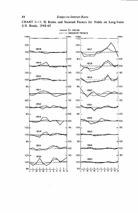
U.S. TREASURY SECURITIES. Chart 2-13 plots the seasonal factors andSI ratios for long-term U.S. Treasury securities (the scale is twicethat used for short-term securities). The pattern prior to 1953 is very
- - 95
1950 -- - 105
1951
100
- - 95
1952
- -105
100
95
- 1956 —
84 Essays on interest. RatesCHART 2—13. SI Ratios and Seasonal Factors for Yields on Long-TermU.S. Bonds, 1948—65
SI ratiosSeasonal factors
Index Index110
105
1948—
Index
105
100
Index
105
100
95
105
100
95
105
100
95
105
100
95
105
100
95
105
100
95
I 11111 liiiJFMAMJJASOND FM AMJ J AS

Seasonal Variation of Interest Rates 85
similar to the early pattern of commercial paper rates, the peak com-ing in midyear and the trough in the fall. Although the amplitude issmall, the pattern is quite real. The reason for the asserted realityresides not only in the similarity between the curves connecting theSI ratios and the ones connecting the factors but also in the positionof the factors, falling as they do between the SI ratios and the 100.0level. The latter result is most conspicuous for 1951 and has theeffect of both dampening the adjusted series and minimizing the possi-bility of the adjustment contributing to the random fluctation of theseries. As in the case of the Treasury bill rates during the late fifties,the assurance that all that is removed is seasonal comes at the expenseof understating what seasonal influence there is. The data for 1952provide a good example of the dilemma involved in adjusting a serieswith a rapidly shifting pattern: the two curves are virtually unrelated.Use of the estimated factors may then introduce random errors intothe series. In 1953 the pattern assumes the shape of the average pat-tern of Table 2-9 and, hence, the high correlations in Table 2-7 be-tween the long-term Treasuries and the other securities. In the follow-ing years the pattern rapidly bends into the one typical of all therates in the late fifties. Even in this period the fit is not very good,although the pattern is clearly there; and the amplitude is among thehighest of the long-term security groups. One notices, even in the latefifties, how the low part of the pattern is gradually extended throughthe summer, as with the short-term securities. By 1965 the pattern isvery different from the average pattern and, in fact, inversely corre-lated with those of most of the long-term series (Table 2-8). It isclear, then, that the low F statistic noted earlier for this series is dueboth to a constantly shifting pattern resulting in a mediocre fit and anunstable pattern even within the periods it describes. That a seasonalpattern existed in the late fifties and even that a systematic ripplepersisted to the end of the study period is, in this study's view, es-tablished. Whether there is reasonable cause to adjust the series Out-side the 1955—59 period is somewhat dubious; and whether it wouldbe meaningful to adjust a series for such a short period is equallydubious. This series is perhaps one that may be profitably left alone.
Chart 2-14 plots the seasonal factors and SI ratios for U.S. Treasurysecurities with three- to five-year maturities. There is a fairly clearpattern for the years 1948—60 followed by several years of erraticmovement—the pattern for 1953 is typical. In 1955 the patternassumes the shape it maintains for the remainder of the decade. In

SI rQtios— Seasonal factors
Index Index Index110 1
86 Essays on interest RatesCHART 2—14. SI Ratios and Seasonal Factors for Yields on U.S. Goyern-ment Three- to Five-Year Securities, 1948—65
48
901949—
Index
110
110-S. — — •_ —
-
RJU
90
ICC1950
90
110-
- 1951110
- 90
100
-11090-
110-
100
- 90
90- —110
100
110- -90
I I I I I I I I I I
J EMAM J J ASO NDthis period the seasonal amplitude of this series is somewhere betweenthe typical amplitude of short- and long-term securities. From 1960on, however, the seasonal pattern is too unstable to justify an adjust-ment.

120 Essays on Interest Rates
(such as income and expected changes in the price level) that de-termine demand are fixed, the demand curve is itself fixed, and theobserved changes in interest rates and money supply may be read aspoints along a given demand curve. The method breaks down, how-ever, when the same variables influence both the demand and the supplycurves (such as, the preponderance of the common cyclical com-ponent in the variables affecting both curves).60
The study of seasonal behavior in the money market partly alleviatesthis problem for two reasons: (1) The use of the ratios-to-movingaverage of the relevant variables, or the smoothed seasonal factors,abstracts from the common cyclical component. This method is, ofcourse, not peculiar to seasonal analysis. More importantly, (2) sea-sonal fluctuations in the demand for money are probably fairly stableover time; so that the seasonal shift in demand relative to the cyclicalcomponent of the shift from, say, November to December is relativelystable from year to year.°7 These seasonal shifts are determined byeconomic forces outside the control of the monetary authorities. Shiftscretion in the matter of seasonality and would bias the estimated elasticity ofdemand for credit, since a simultaneous solution would be required. I am in-debted to Walter Fisher for this point.
Using averages for cyclical stages Cagan is able to show an inverse rela-tionship between interest rates and changes in the money supply. (See hisChanges in the Cyclical Behavior of Interest Rates, Occasional Paper 100, NewYork, NBER, 1966; reprinted as Chapter 1 of this volume.) Note he relateschanges in money supply to levels of interest rates; whereas this study dealswith seasonal changes in both series.
Since demand per se is not observable, this proposition must be hypothe-sized rather than demonstrated. Some evidence in support of the propositionlies in the absence of any systematic variation in the seasonal amplitude ofGNP within the study period. The implicit seasonal factors for the fourthquarter, the period of peak seasonality in the GNP, are given below. The rawdata, of adjusted and nonajjusted series, are given in The National Income andProduct Accounts of the United Slates, 1929—1965, pp. 11 30.
Implicit Factors f,nplicit FactorsYear Fourth Quarter Year Fourth Quarter
1948 107.2 1957 106.01949 106.7 1958 105.91950 ]0$.7 1959 105.9
1951 1960 105,8
1952 105.6 1961 105.8
1953 1962 105.9
1954 105.6 1963 105.8
1955 105.3 1964 105.6
1956 105.9 1965 106.6

Seasonal Variation of Interest Rates 119supply of short-term credit in November results in a given interestrate, RN. In December there is an increase in the demand, depictedby the outward shift in the demand curve. If the Federal Reserve didnot increase the supply at all—that is, in the present context, if therewere no seasonal movement in the money supply—the rate of interestwould rise to At the other extreme, if the Federal Reserve hadfully anticipated the rise in demand and increased the supply of moneycorrespondingly (to S0), the rate of interest would remain at RN. Again,in the present context that would imply a relatively greater seasonalamplitude in the supply of money. Finally, if the Federal Reserveanticipated part but not all of the increase in demand, the rate wouldmove to some intermediate position—say, The necessary seasonalamplitude in the supply of money to effect any given interest, rateclearly would depend on the elasticity of demand for short-term credit:The more elastic the demand for short-term credit is with respect tothe interest rate, the greater must be the seasonal amplitude in monetsupply necessary to prevent the seasonal increases in demand fromimparting a seasonal variation to interest rates.
But how sensitive is the demand for short-term credit to the interestrate? Conversely, how sensitive is the interest rate to variations inthe supply of money? Discussions of these questions typically bogdown in the identification problem—that of distinguishing shifts inthe demand curve from movements along it. In practice one can onlyobserve the change in the interest rate and the change in the moneysupply as of a given time. Since the demand curve is itself varying,there is no sure way to associate the given readings of interest rateand money supply with a particular demand curve and, therefore, toascertain the elasticity of the curve. The problem is soluble insofaras it is feasible to specify the variables that determine the demandcurve and to fix these variables while allowing the variables affectingthe supply curve65 to move freely. In this situation, since the variables
05 Since the supply of new money is largely at the discretion of the FederalReserve, to this extent the variables that affect the supply curve are those thataffect the Federal Reserve's decision. This analysis presumes an autonomouslydetermined supply of money. To the extent that the supply of money respondsto interest rates apart from Federal Reserve activity, the purported separationin the determinants of supply and demand breaks down. While this point mayweaken the analysis, the elasticity of supply with respect to interest rates is notlikely to be sufficient to negate the substance of the analysis. In either case, theseasonal in interest rates depends on the seasonal in demand relative to supply.An endogenous supply would lessen the importance of Federal Reserve dis-

118 Essays on interest Ratesthe Federal Reserve's policy of adjusting the supply to the seasonalchanges in the demand for short-term credit.°3 The series on totalbills outstanding is discussed later. However, if this policy were com-pletely successful,64 there would be no seasonal in interest rates.Figure 2-2 hypothetically depicts the situation. The demand for and
Interestrate
03 The present section considers the monthly changes in the money supplysynonymous with changes in the supply of short-term credit. The appendix tothis section deals briefly with this subject to help evaluate the findings of thissection.
The supply series used in this study conforms to the narrow definition ofpublicly held currency and demand deposits. Since time deposits do not havea significant seasonal, the broad definition of money should yield similar results;the seasonal components of both series are very similar.
04 The word "success" is artificially vital in the current context, since theFederal Reserve did not necessarily intend to smooth out the seasonal variancein short-term rates. The desirability of eliminating the seasonal influence oninterest rate is discussed in Friedman and Schwartz. op. cii., pp. 292—296.
Rp
R0
upply in November
in December
in December
emcind in November
FIGURE 2-2Number' dollars
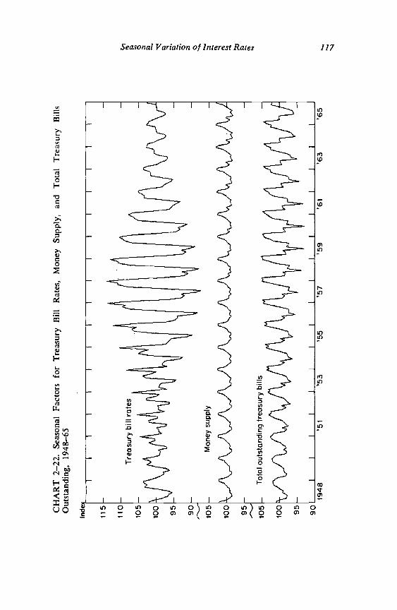
CH
AR
T 2—
22. S
easo
nal F
acto
rs fo
r Tre
asur
y B
illR
ates
, Mon
ey S
uppl
y, a
nd T
otal
Tre
asur
y B
ills
Out
stan
ding
, 194
8—65
-s -S I.- -S

116 Essays on Interest Ratesthe reduced arbitrage, at cyclically high rates—a consideration thatis apparently offset by the one noted earlier.
Aside from the cyclical effect, however, the incentive to arbitrageis influenced by the Federal Reserve's policy toward seasonal changesin the demand for credit. The Federal Reserve's failure to meet thepeak demand for credit in December would by itself produce a risein the bill rate both directly through its own operations and indirectlythrough the effect on the borrowing costs of arbitraguers. Similarly,its failure to absorb redundant credit in June and July would preventthe arbitraguers' sales (to effect their capital gain) from driving therates up. Admittedly, the failure to contract the credit supply, or moregenerally to diminish its rate of increase, during June and July wouldincrease the incentive to arbitrage. This policy combined with an easycredit policy in December would, of course, lower the level of rates;but it would not eliminate the seasonal variance. Alternatively, the at-tempt to keep short rates high by contracting the credit supply in Julyand taking no action at other times would simply diminish the incen-tive to arbitrage and raise the December peak. In effect, it is a tightcredit policy, which affects the level of rates but not the seasonality.'32To counter the seasonal movement in interest rates, as distinct fromthe level of rates, requires, therefore, a relatively easy policy in De-cember and a relatively tight one in July. The seasonal pattern in themoney supply should therefore correspond with the pattern in short-term interest rates, as in fact it does. But the seasonal amplitude inmoney supply (that is, the extent to which the Federal Reserve alter-nates the relative tightness and ease) should be inversely related tothe seasonal amplitude in short-term interest rates: The more theFederal Reserve equilibrates the supply with the demand for short-termcredit, the less will interest rates vary. The final section of this reportinvestigates this relationship.
The Eflect of the Seasonal Amplitude of the Money Supply
Chart 2-22 plots time series of the seasonal factors for Treasury billsand money supply, and total bills outstanding. The relative lows inJune and July and the highs in the fall months are clear evidence of
2 In both cases the change is In the over-all level of rates but not the intra-month relations. By allowing the rates in December and July to fall by thesame amount, the moving average is lowered and the December peak main-tained. This point in a related issue was discussed in Section II.
Seasonal Variation of Interest Rates 115
Since seasonal amplitudes should depend inversely on the slope, theyshould also be inversely related to the level of. rates, or at least thelevel in relation to that of adjacent years. In Section III, we found nosuch relation in the data themselves. It may be, however, that thisproposition works to offset a tendency in the opposite direction: Inperiods of tight money, during cyclical highs, it is harder or morecostly to borrow money in order to arbitrage the seasonal movement.Consideration of this point concludes this section of the study.
There are as many ways to arbitrage the seasonal influence inshort-term rates as there are combinations of relevant maturities. Thefollowing discussion arbitrarily selects nine- and three-month securitiesand deals only with the peak-to-trough and trough-to-peak relation-ships;• although, in principle, arbitrage is feasible between any pairof months.°° The rule in seasonal arbitrage is simply to borrow cheaplyand lend dearly; that is, borrow in July and lend in December. Thereare two ways to effect the transaction: Borrow and sell a nine-monthsecurity in July at high prices and cover the short sale in Decemberat low prices. Alternatively, buy a nine-month security in Decemberand sell it, now a three-month security, the following June. The termstructure would work against the arbitraguer in the first alternativeand for him in the second.61
Given the seasonal spread, the incentive to arbitrage is determinedby the cost of borrowing. In periods near cyclical peaks the incentiveto purchase nine-month securities in December in order to sell themthe following June is limited by the higher borrowing cost. On thisground one might expect a greater seasonal amplitude, because of
In this connection, the smoothness of the seasonal patterns of interest rates,'i.e., the absence of abrupt changes between adjacent months, is understandable.The major cost of seasonal arbitrage is borrowing cost, which is, of course, alinear function of the length of the loan. It is cheaper to arbitrage betweenadjacent months than across' a six-month period, but the smoothness of thepattern reduces the opportunity. Whether the opportunity decreases at a fasterrate than the costs as the span of the transaction decreases is determinable forany specific case.
In addition, short positions are more costly to finance than long positions.The borrower must pay 1/2 of 1 per cent of the value of the security (annualrate) plus the interest that accrues to the security. See A Study of the DealerMarket for Federal Securities, op. cit., p. 20. Moreover, the margin require-ment is much greater on a short position than on 'a' long position: aboutper cent compared with of I per cent on a long position in certificates(ibid., p. 92). It is unlikely, therefore, that this method of arbitrage wouldrecommend itself for smoothing seasonal differentials.

114 Essays on Interest Rates
each year for the months June through November are given inTable
As much as this analysis accurately depicts one aspect of theseasonal problem it implies still another. Typically, though not always,the slope of the yield curve is greatest when the level of rates is low.59
TABLE 2-15. Differential in the Trend-Cycle Values Between Nine- toTwelve-Month and 91-Day Treasury Securities for June Through November,1948—65 (basis points)
Year June July August September October November
1948 6 10 13 14 12 111949 —4 12 8 6 5 41950 0 3 8 4 5 51951 24 10 10 9 10 111952 —1 —7 5 17 13 41953 11 18 23 24 42 171954 1 —7 —13 —12 —2 121955 30 14 15 11 4 131956 11 27 25 26 25 23 .
1957 13 29 38 • 43 31 231958 44 54 19 —5 2 301959 74 78 93 67 66 701960 71 62 65 51 53 551961 44 53 50 71 64 551962 25 0 16 22 19 111963 14 9 6 13 14 231964 15 16 22 23 23 221965 11 9 16 14 14 23
NOTE: The figures are trend-cycle values for nine- to twelve-month securitiesminus trend-cycle values for 91-day bills. The figures indicate the slope of the yieldcurve in the designated range independently of the seasonal and irregular movements.For the present purposes the differential in the seasonally adjusted rates (that is,including the irregular component) is a relevant alternative to the figures presentedhere.
In the jargon of the expectations hypothesis, when current rates are belowtheir normal or typical values they are expected to rise. Longer-term lendersrequire a higher yield in compensation for the expected capital loss. The con-cept is analogous to the one underlying the Keynsian liquidity preference func-tion. Admittedly, the figures in Table 2-15 do not cast a very favorable light onthis hypothesis; although, most sets of term structure data support it. ReubenKessel, op. cit., argues that the very short-term part of the yield curve is domi-nated by liquidity premia which, he argues, are positively related to the levelof rates.

Seasonal Variation of Interest Rates 113
therefore avoided the Treasury Bulletin data. The data do, however,illustrate this section's argument. A direct test for the relation betweenthe seasonal amplitude of one-month rates in December and the non-seasonal yield differential between two- and one-month rates in Novem-ber is available, simply, in a regression of the SI ratios for one-monthbills in December on the differential in the trend-cycle components oftwo- and one-month rates in November. The correlation coefficient ofthis regression is .56; the regression coefficient, 53.56; and its t-value,2.68. In general, the variance of the SI ratios for a given year (thatis, the extent of seasonal amplitude) is directly related to the slopeof the yield curve.57 The converse is also true: the unadjusted term-structure data partly reflect the seasonal pattern—which was Macaulay'spoint.
The point is again manifest in the nonseasonal differential betweennine- to twelve-month Treasury securities and 91-day Treasury bills.The average differential in July58 is considerably greater during theperiod of peak seasonality, 1955—61, than during the earlier or laterperiods. In the period 1948—54, the mean differential in the trend-cycle values of nine- to twelve-month and 91-day Treasury securitieswas 6 basis points; in the period 1955—61, 45 basis points; and in1962—65, 9 basis points (all figures are for July). The figures for
It is obviously necessary to work with the SI ratios, preferably modifiedfor extremes, instead of the seasonal factors themselves since the factors aredesigned to smooth out the effects of year-to-year changes in seasonal amplitude.In other words, to the extent the above analysis is relevant, the X-1 1 methodof seasonal adjustment is inappropriate. There is nothing sacred about theDecember figures. In fact, the SI ratios of all seasonally high months arepositively related to the slope of the yield curve, and those of all seasonallylow months negatively related. In other words, the seasonal amplitude as awhole is positively related to the slope of the yield curve. While the relationfor the seasonally high months is understandable, its application to the lowmonths is less clear. Even if the principle stated in the text applied only to thehigh months, the observed effect on the low months would obtain due to theeffect of the high months on the trend-cycle curve. This point is considered inSection II.
July replaces November in this calculation because of the difference inmaturities involved. Here the borrower, say the U.S. Treasury, avoids the three-month peak rate in December by borrowing for nine months in July insteadof for three months in December, perhaps simultaneously purchasing a six-month security to effect the forward loan. Curiously, the point in the text ismost true for July, when the combination of nine- and three-month securitiesis appropriate to the December peak; although, to a lesser extent it applies toall the months.

112 Essays on Interest Ratesspan forecasts, for which they have more information, than their longerspan forecasts, for which they are likely to rely more on extrapola-tions.55
In evaluating the empirical basis for the expectations hypothesis,Macaulay found evidence of market forecasting in the fact that theseasonal peak in yields on time loans preceded the peak in call loans.50Banks, he said, aware of the seasonal peak in call money rates duringDecember, would not tie up money in, say, November, without insur-ing a return comparable to the average return on call money duringthe two months. The yield on time money would therefore peakearlier. With respect to this phenomenon, its amplitude would have tobe smaller, as well. Consider the same phenomenon from the borrow-er's point of view: To avoid the December rush he can borrow inNóvëmber for two months, perhaps lend the money for one month,and in effect acquire a forward loan for December at the lower Novem-ber rate. These transactions would have the effect Macaulay observed,in addition to smoothing the one-month seasonal. But the borrower'sability to avoid the peak rate depends on the nonseasonal relation be-tween the two-month and one-month rates in November. If the formerwere much greater than the latter, both rates adjusted for seasonality,what the borrower gains by avoiding the seasonal he loses in the termstructure differential. Since this differential is known in November, itin part determines the extent of the seasonal arbitrage and, therefore,of the seasonal amplitude itself. This analysis, thus, suggests that arelation exists between the slope of the yield curve and the seasonalamplitude.
Testing for this relation obviously requires data for different butproximate maturities. The Treasury Bulletin publishes series on one-,two-, and three-month Treasury bills, but these data record the yieldson the last trading day of the month instead of weekly averages, asin the Federal Reserve Bulletin's series on 91-day Treasury bills. TheTreasury Bulletin's series therefore have a considerably greater randomcomponent distorting the estimated seasonal patterns. This study has
There are, in addition, various eclectic theories of the term structure. Theliterature on this subject has grown in recent years—much more, unfortunately,than. our knowledge. Two standard works are: David Meiselman, The TermStructure of Interest Rates, Englewood Cliffs, N.J., 1961; and Reuben Kessel,The Cyclical Behavior of tile Term Structure of Interest Rates, Occasional Paper91, New York, NBER, 1965, and reprinted as Chapter 6 of this volume.
Op. cit., p. 36. Kemmerer, op. cit., p. 18, observed the same phenomenonand had the same explanation for it.

Seasonal Variation of Interest Rates Illmeasure of risk premium.54 While this suggestion helps to illustrate thepotential uses of time series decomposition, it suffers from the sameproblem this study emphasized throughout: the difficulty in distinguish-ing variations in seasonal amplitude from irregular movements.
Short-Term Securities
While the cost-return analysis of seasonal arbitrage applies equallywell to short- as to long-term securities, the calculation of the costcomponent is complicated by the greater yield differentiation amongproximate maturities at the short-end of the yield curve. Whereas thenonseasonal components of the yields on twenty- and nineteen and ahalf-year securities are approximately the same and therefore do notaffect the arbitrage, a substantial differential between a one-month anda two-month or a nine-month and a three-month security may offset anyseasonal differential. The calculated costs of arbitrage must, therefore,take account of the former differential.
The tendency for yield curves, the curves relating yield to maturitywith maturity, to incline at a diminishing rate is a widely observedphenomenon and its explanation a subject of considerable dispute. Somewriters attribute the phenomenon to the greater number of investorswith short-term liabilities who to match the maturities of theirassets and liabilities than investors with long-term liabilities havingsimilar preferences—the so-called hedging theory. Others emphasize in-vestors' preference for short-term securities to minimize their vulner-ability to capital losses—the liquidity preference theory. In either caseyields increase with maturity to equilibrate supply and demand. Finally,the expectations hypothesis associates the yield structure with in-vestors' expectations of future interest rates. While this theory doesnot account for the observed average incline in the yield curve, it canaccount for the greater differentiation among shorter term yields byrecognizing the greater differentiation of investors among their shorter
In this context there is no need to consider differences in cyclical variation,which could further account for aggregate yield differentials ainong the varibusgroups of securities, since the seasonal and irregular components abstract alikefrom the cyclical components of all the series. In principle, this measure ofrisk premium captures the true relation between the relative dispersion ofyields and the yield differential of competitive securities as distinct from differ-ences in the expected yields of the securities.
110 Essays on Interesi Rateslocal issues. This point may account for the difference in the longevityof the seasonal amplitude in the two sets of securities, but the studymakes only a prima facie case for the issue.
The illustrative example implies that, contrary to common opinion,there is nothing in investment behavior to preclude a seasonal influenceon long-term rates provided its amplitude is sufficiently low. Sinceseveral years are required before investors perceive a seasonal, virtuallyany amplitude is possible for a limited period. The low breakeven pointsfor eliciting arbitrage, 0.10 per cent and 0.14 per cent, for 5 per centand 25 per cent margin requirements, respectively, computed in theexample no doubt understate the true values because of additional busi-ness costs not incorporated in the example, as well as the point, notedin the introduction, that arbitrage is in effect at one extreme—speculationis at the other—of a continuum as the certainty of the differential be-tween two situations becomes more remote.5'
Perhaps the greater seasonal amplitude of municipal securities isexplained by the greater prominence of their irregular components. It istempting to generalize this point—the direct relation between seasonalamplitude and relative importance of the irregular component—into anhypothesis. Other influences on these variables, combined with the factthat the seasonal and irregular components are not independently esti-mated,52 would tend to obscure the relation, however. Yet we do findthat the rank correlations between the ratio of the variance of the ir-regular component to that of the whole series (Table 2-4, column 1)and the seasonal amplitude as measured by the variance of the factors(Table 2-5) increases from the earliest to the latest years.53 The in-creasing correlations imply a movement toward an equilibrium trade-offbetween yield and certainty of principal. In the absence of other causesof seasonal differences among long-term securities, the observed differ-entials in seasonal amplitude combined with the observed differences inthe relative importance of the irregular component would produce ameasure of the rate of trade-off between the two or, in other words, a
In this regard it would be better to replace at least in principle theseasonal factors in the illustrative example with confidence intervals or perhapssome form of certainty equivalents.
In fact, the bias in the computation is toward• an inverse relation, whichstrengthens the conclusion.
the years 1953, 1957, 1963, and 1965, the rank correlation coefficientsare .30. .59, .76, and .82, respectively. These figures exclude the two long-termTreasury securities, although there was no attempt to determine how theirinclusion would affect the results.

Seasonal Variation of Interest Rates 109TABLE 2-14 (concluded)
Part B: $5,000 Invested With 25 Per Cent Margin Requirement
Costs
Foregone interesta on $5,000 for sixmonths at assumed annual rate of5 per cent .025 x 5,000 = $125.
Transactions cost (buy and sell)at assumed $5 per $1,000 bond 5 X 20 = 100.
Interest cost of borrowed money forsix months at assumed rate of1 percentage point above bond yield .5 X .01 x 15,000 = 75.
Total cost = $300.
Returns
Price differential (between Septemberand March) at assumed $10.70 per$1,000 bond for each .1 per cent ofseasonal factor 20 X 10.70 = $214.
Required seasonal factors to cover cost 100 + X .1 =100.14%
100 .1 = 99.86
aThe capital on which the foregone interest is computed should include half thetransactions cost and approximately half the borrowing cost. The greater accuracy,however, will not significantly improve the estimates.
an increasing term to maturity, since the longer the term the sooner willa given seasonal amplitude invite arbitrage. This point may explain thegreater amplitude in three- to five-year Treasury securities than in theequivalent long-term securities and in the Treasury bill rates than in thenine- to twelve-month securities, it may also help explain the smalleramplitude of commercial paper rates, which are often six months tomaturity, than in the short-term yields on bankers' acceptances and on91-day Treasury bills.
While margin requirements vary over time and among borrowers,they are always lower for Treasury securities than for private and state-

108 Essays on Interest RatesTABLE 2-14. Costs and Returns of Arbitrage for Twenty-Year SecuritiesBetween Seasonal Peaks and Troughs Under Certain Hypothetical Conditions
Part A: $5,000 Invested With 5 Per Cent Margin Requirement
Costs
Foregone interesta on $5,000 for sixmonths at assumed annual rate of5 per cent .025 X 5,000 = $125.
Transactions cost (buy and sell) atassumed $5 per $1,000 bond 5 X 100 = 500.
Interest cost of borrowed money forsix months at assumed rate of1 percentage point above bond yield .5 X .01 X 95,000 = 475.
Total cost = $1,100.
Returns
Price differential (between Septemberand March) at assumed $10.70 per$1,000 bond for each .1 per cent ofseasonal factor 100 X 10.70 = $1,070.
1,100Required seasonal factors to cover cost 100 +1 070
X .1 =100.10%
100—
X .1 = 99.90
(continued)
cent margin requirement the seasonal factors must exceed 0.10 per centon either side of the level of rates to just cover the arbitrageur's costs.(While the example does not illustrate the point, it is also true that thegreater the term to maturity, the greater the effect on the price differentialof any given differential in yield.) When the margin requirements rise to25 per cent, the required seasonal factors are 0.14 per cent on either sideof the level of rates to just cover costs.
The long-term series considered in this study do not differentiateamong terms to maturity; therefore, this study did not estimate therelation between term to maturity and the breakeven seasonal factors.However, one certainly expects the seasonal amplitude to diminish with

Seasonal Variation of Interest Rates 107average price over the year is the $1,000 par value. Assume aninvestor purchases the bond at its seasonally peak yield in Septemberand sells it, now with nineteen and one half years to maturity, thefollowing March when yields are at their seasonal trough. The presentvalue formula computes the prices in September and March for anydesired seasonal change in yield in the following way:
20 20 20. + 1000September pnce = (1.02 P.F.) + (1.02 P.F.)2 + (1.02
P.F. = peak seasonal factor, e.g., 101.0; T.F. = trough sea-sonal factor, e.g., 99.0; semiannual coupon payment is $20; principalis $1,000; and average yield is 2 per cent per half-year.
The computation leads to the result that for each one-tenth of 1 percent in the seasonal amplitude on either side of the average value (inother words, factors equal to 100.1 and 99.9 for September and March,respectively) the price differential for a $1,000 bond comes to approxi-mately $10.70. For an amplitude of two-tenths of a per cent (i.e., 100.2and 99.8), the price differential is approximately $21.40.
To estimate the seasonal amplitude necessary to encourage arbitrage,this study estimated the costs and returns to this activity in two hypo-thetical situations: $5,000 is invested with a 5 per cent and with a 25per cent margin requirement. In the first case the investor borrows$95,000 and purchases $100,000 worth of bonds; and in the second case$15,000 and purchases $20,000 worth of bonds. Table 2-14 lists theestimated costs in the two situations under the following assumptions:
—Foregone interest on $5,000 at annual rate of 5 per cent—Transaction cost is $5 per $1,000 bond for combined buy and sell—Interest cost of borrowed money exceeds bond yield by 1 per-
centage point per
The required peak and trough seasonal factors are computed for break-even, account being taken of the opportunity costs of the investment.
While the estimated returns obviously depend on the conditions as-sumed to prevail, the orders of magnitude are established. The smallerthe margin requirements, or obversely, the greater the amount borrowedrelative to capital, the smaller is the seasonal amplitude required toproduce the breakeven price differential. In the example, with a 5 per
The greater the difference between the long and short rate the greater isthe incentive to arbitrage.

106 Essays on Interest Ratesparticular time; but when the two situations occur in different periodsthe knowledge of the later period is at best a good forecast. The un-stable character of the seasonal influence on interest rates revealed inSection III implies that using •the term arbitrage in connection withseasonals is somewhat misleading. Certainly, arbitrage shades intospeculation as the seasonal movement becomes more problematic.
The last part of this section relates changes in the seasonal ampli-tude of Treasury bill rates with corresponding changes in the sea-sonal amplitude of other series.48 The seasonal amplitude of Trea-sury bill rates is inversely related to the seasonal amplitude of the stockof money and directly related to that of total bills outstanding. Thisfinding, relevant in its own right as a description of events, servesalso to illustrate the usefulness of decomposing a series to help ex-plain its behavior. For example, when the aggregate series of interestrates and money supply are correlated, the expected inverse relationis usually obscured by the common effect of economic activity on thecyclical components of both series; although the series frequently turnat different stages of the cycle, there are many periods during whichthe series are moving in the same direction. However, when thecyclical component is filtered out, the expected inverse relation ma-terializes. By replacing the original series with their seasonal factors,this study estimates the elasticity of short-term demand for creditwith respect to interest rates to be a very small but statistically sig-nificant
Arbitrage
Long-Term Securities
To determine the opportunity for arbitrage between seasonal phases,this study computed the effect on buying and selling prices, under aset of assumed conditions, of various seasonal amplitudes. Considera twenty-year, 4 per cent bond with semiannual coupons whose
£8 "Seasonal amplitude" refers to the average departure of the monthly factorsfrom 100.0. When the pattern of factors is approximately constant from yearto year the change of a given month's factor from one year to the next is ameasure of the change in seasonal amplitude.
The appropriateness of the concept of elasticity in the present context isevaluated in a brief appendix to this section.

Seasonal Variation of Interest Rates 105
implicit factors, as well as the Kuznets factors, are plotted against theSI ratios. The implicit factors appear to follow the SI ratios slightlybetter than do the original factors; whether they are therefore pref-erable is a question on which one can argue both sides. Althoughthe double adjustment method is used in this study for illustrativepurposes, further experimentation may demonstrate its usçfulness asa method of adjustment when there are abrupt changes in the sea-sonal amplitude. Whether the single or the double adjustment is pre-ferred there is no compelling reason to reject the machine adjustmentfor any part of the sample period, although some users may preferto take the adjusted data back only to about 1953.
IV. DETERMINANTS OF SEASONAL AMPLITUDE
This section considers some topics related to the extent and varia-tion of seasonal amplitudes. One of the topics it deals with is theprofitability of arbitrage between periods of seasonally high and lowyields on long-term securities. It was found that, taking account ofdirect transactions and opportunity costs, a relatively small seasonalwould elicit arbitrage—the more sq the longer is the term to maturity,the smaller the margin and the greater the stability ofthe seasonal. The breakeven point for profitable arbitrage, estimatedthrough use of hypothetical though plausible data, is the sea-sonal amplitude that actually persisted through most the studyperiod. The result implies that a high risk premium isattached to the uncertainty with the seasonal regarded, aswell as the expected dominance of the and com-ponents. The breakeven seasonal for risk thereforebe much larger. Consideration of and .bother costs of anarbitrage operation would also raise the point.
The greater importance of term structure on short-term yield differ-entials complicates the question of arbitrage in the short-term segmentof the securities market. Several authors have observed that the sea-sonal patterns of some short-term securities lead those of shorter termsecurities. Since these leads are evidence of investors' awareness ofthe seasonal movement and more generally of their attempt to fore-cast short-term rates, they are also evidence of what this study is call-ing arbitrage. Arbitrage generally implies bridging a known discrep-ancy between two situations, usually between two markets at a

104 Essays on Interest Rates2—21. SI Ratios, Original and Implicit Seasonal Factors, andFactors for Treasury Bill Rates, Selected Years
_____
SI ratLos————OrLgLnaI seasonal factors
Implicit factors
CHARTKuznets'
SI ratios—— — — Kuznets' factors
Index130
Index
120
110
100
90
80
120
110
100
90
80
110
100
90

Seasonal Variation of Interest Rates 103CHART 2—20. Unmodified SI Ratios, Original and Implicit Seasonal Fac-tors, and Kuznets' Factors for Treasury Bill Rates
Unmodified St ratios
Kuznets' factors
IrTiplicit seasonal factorsOriginal seasonal factors
Unmodified S I ratios
uznets' factors
seasonal factorsseasonal factors
December

t'j
TA
BLE
2-13
. Sea
sona
l Fac
tors
of T
reas
ury
Bill
Rat
es fo
r Sel
ecte
d Y
ears
Com
pute
d fo
r the
Orig
inal
and
the
Seas
onal
lyA
djus
ted
Serie
s, an
d th
e K
uzne
ts' M
etho
d
1953
1958
1965
Orig
inal
Adj
uste
dIm
plic
itK
uzne
tsO
rigin
alA
djus
ted
Impl
icit
Kuz
nets
Orig
inal
Adj
uste
dIm
plic
itK
uzne
tsM
onth
(1)
(2)
(3)
(4)
(5)
(6)
(7)
(8)
(9)
(10)
(11)
(12)
Jan.
102.
198
.910
1.0
102.
310
8.9
101.
611
0.6
112.
310
2.3
99.7
102.
010
1.1
Feb.
97.0
98.5
95.6
100.
098
.499
.998
.398
.110
2.0
100.
510
2.5
99.9
Mar
ch99
.210
0.8
100.
098
.992
.198
.490
.691
.810
0.8
101.
710
2.5
99.3
Apr
il98
.910
1.1
100.
098
.691
.098
.189
.389
.799
.310
1.4
100.
699
.2M
ay98
.710
0.7
99.4
98.5
92.6
95.0
87.9
89.4
97.9
101.
499
.399
.1Ju
ne94
.910
0.1
95.0
97.3
89.4
99.7
89.1
81.9
97.3
101.
498
.798
.5Ju
ly94
.410
3.1
97.3
97.1
87.9
99.1
87.1
80.4
98.0
101.
999
.998
.3A
ug.
102.
910
2.2
105.
299
.996
.299
.796
.097
.899
.810
0.7
100.
199
.9Se
pt.
103.
998
.910
2.7
102.
010
7.4
100.
410
7.8
110.
599
.897
.797
.410
0.9
Oct
.10
1.3
99.2
100.
610
2.0
110.
610
1.7
112.
511
0.5
100.
097
.397
.310
0.9
Nov
.10
0.0
97.7
97.7
101.
911
0.9
102.
811
4.0
110.
110
0.1
97.9
98.0
100.
9D
ec.
108.
499
.410
7.8
103.
811
3.0
102.
411
5.8
121.
610
2.6
98.3
100.
910
1.9

Seasonal Variation of Interest Rates 101
original factor in column 1. Conversely, when the factor in 2 is below100.0, the original estimate is too high (i.e., the seasonal trough un-derestimated) and the factor in 3 is below the factor in 1. When thefactor in 6 is below 100.0, the original estimate of the seasonal peakis exaggerated and correspondingly reduced in 7; when above theoriginal estimate it is too low and therefore increased in 7. From1956 to 1960 the machine understated the seasonal low in July.Some, but very little, seasonal low remains in the adjusted data. Inthe other years, however, the machine converted the original sea-sonal lows in the July data to seasonal highs46 in the adjusted data.In December the seasonal from 1954 to 1960 is understated in theoriginal adjustment and in the remaining years overstated.
Table 2-13 puts the same story a little differently. In 1953 thefactors computed in the second adjustment (column 2) denote, withsome exceptions and with a smaller amplitude, seasonal movementsin the opposite direction from those implied in the original adjust-ment. In 1958, the seasonal timing implied in both columns 5 and 6is the same, reflecting the original adjustment's failure to fully re-move the seasonal variance in the original series. In 1965, again thedirections are reversed.
While these results confirm the expected faultiness in the machine'shandling of a moving seasonal component, they emphasize even morethat the magnitude of error is usually quite small; for the bill rate,with one exception, it is never more than 3 per cent of the originalseries and usually much less." However, during the peak period theKuznets factors differ from the original X-1 1 factors by up to 7percentage points. The order of magnitude involved is shown inChart 2-20 and again in Chart 2-21, where both the original and the
"High" and "low" denotes positions above and below 100.0, respectively;"peak" and "trough" denotes highest and lowest, respectively. The. Kuznetsexperiment implies the same result for July but dates the period of under-statement in 1956 instead of 1954 for December.
The F test for stable seasonality in the second adjustment indicatesinsignificant seasonality at any level. In adjusting the adjusted data, the machineconfronts the same problem of a moving seasonal and therefore similarly under-estimates the extent of the original maladjustment. The magnitudes involvedthere, however, are small, and one may safely ignore this point. In fact, theopposite danger exists that the machine may confuse the relatively muchgreater irregular component with the seasonal one and exaggerate the extentof the original maladjustment. There is no justification, for example, for theimplicit lows in September, October, and November of 1965 (column 11,Table 2-13).
100 Essays on Interest Rateswith the Kuznets method.44 These factors are simply the computedvalues of the regressions described earlier. The X-11 factors (columnsI and 5) clearly dampen the changes in seasonal amplitudes. Ex-cluding 1948 and 1949, the Kuznets factors show larger seasonalamplitudes from 1956 through 1960 than the X-1 1 factors andsmaller amplitudes elsewhere. The differences are greatest in 1957and, expectedly, in 1958. Whereas the X-11's July factors for theseyears ai:e, respectively, 87.4 and 87.9, the corresponding Kuznetsfactors are 85.0 and 80.4; for December the X-1 1 factors are 113.9and 113.0, respectively, for 1957 and 1958, and the correspondingKuznets factors, 118.7 and 121.6.
The adjustment's sensitivity to abrupt changes in amplitude is notsolely a question of preference. One condition for a perfect adjustmentis the absence of seasonality in the adjusted data.45 Perfection aside,the seasonality that remains in the adjusted data betrays the qualityof the original adjustment. In other words, even allowing a graduallychanging seasonal, the moving average of the X-1 1 may not besufficiently elastic to expunge all the variation that by its own criteria(i.e., its response to a second round) are seasonal. The seasonallyadjusted data will in this case retain some remnants of the seasonalpattern. The experiment with the Kuznets method suggests what theseremnants will Jook like.
To illustrate the point, this study ran the seasonally adjusted dataonce again through the X- 11. Columns 1 and 5 of Table 2-12 list thefactors for July and December, respectively, obtained with the originaladjustment; columns 2 and 6 list the factors with the second adjust-ment; and columns 3 and 6 the implicit factors computed by dividingthe twice-adjusted series (i.e., the series obtained by adjusting theseasonally adjusted series) into the orignal series. When the factor incolumn 2 is above 100.0, the original estimate of the July factor istoo low, that is, the seasonal decline is exaggerated; the implicit factorin column 3 is in this case greater (i.e., closer to 100.0) than the
"The other figures in Table 2-12 and curves in Chart 2-10 are explained below.While necessary, this condition is not sufficient. The adjusted data must
also remain faithful to the original in all respects other than seasonality. Thetrend-cycle values, for example, are free of seasonality but do not otherwisequalify as properly adjusted values of, the original series. Lacking perfection,an adjustment method should evince a convergence toward no-seasonality uponsuccessive adjustments of the data, that is, adjustments of the adjusted data.The X-1 1 appears to satisfy this requirement, although the present study hasnot considered this issue in any detail.

TAB
LE 2
-12.
Sea
sona
l Fac
tors
of T
reas
ury
Bill
Rat
es fo
r Jul
y an
d D
ecem
ber C
ompu
ted
for t
he O
rigin
al a
nd th
eSe
ason
ally
Adj
uste
d Se
ries,
and
the
Kuz
nets
'Met
hod
(per
cen
t)
Jul y
Dec
embe
r
Orig
inal
Adj
uste
dIm
plic
itK
uzne
tsO
rigin
alA
djus
ted
Impl
icit
Kuz
nets
Yea
r(1
)(2
)(3
)(4
)(5
)(6
)(7
)(8
)
1948
96.8
100.
096
.995
.110
3.7
99.8
103.
510
4.9
1949
97.0
970.
997
.896
.910
3.9
99.4
103.
310
3.3
1950
97.3
102.
199
.398
.310
4.6
99.3
103.
810
2.1
1951
96.9
102.
999
.899
.010
5.5
99.1
104.
510
1.4
1952
96.2
103.
599
.698
.110
6.9
99.2
106.
010
2.7
1953
94.4
103.
197
.397
.110
8.4
99.4
107.
810
3.8
1954
92.4
102.
394
.592
.911
0.5
100.
111
0.6
107.
719
5589
.810
0.7
90.5
91.0
112.
210
0.9
113.
211
2.0
1956
88.3
99.8
88.1
87.8
113.
810
2.0
116.
111
4.8
1957
87.4
99.1
86.6
85.0
113.
910
2.4
116.
711
8.7
1958
87.9
99.1
87.1
80.4
113.
010
2.4
115.
812
1.6
1959
89.0
99.0
88.2
85.0
110.
510
1.4
112.
111
5.2
1960
91.1
99.6
90.8
89.9
107.
910
0.3
108.
210
9.8
1961
93.3
100.
293
.595
.910
5.1
99.1
104.
210
4.3
1962
95.3
100.
896
.197
.510
3.5
98.5
101.
910
3.1
1963
96.7
101.
398
.098
.210
2.7
98.3
101.
010
2.2
1964
97.6
101.
799
.398
.310
2.7
102.
698
.410
1.1
102.
019
6598
.010
1.9
99.9
98.3
98.3
100.
910
1.9
C-, 0 0 0 0 0 0 0
NO
TE: C
olum
ns 1
and
5 a
re th
e or
igin
al fa
ctor
s com
pute
d w
ith th
e X
-1 1
. Col
umns
2 a
nd 6
are
the
fact
ors c
ompu
ted
for a
djus
ting
the
seas
onal
ly a
djus
ted
serie
s. C
olum
ns 3
and
7 a
re th
e im
plic
it fa
ctor
s obt
aine
d w
ith th
e do
uble
adj
ustm
ent.
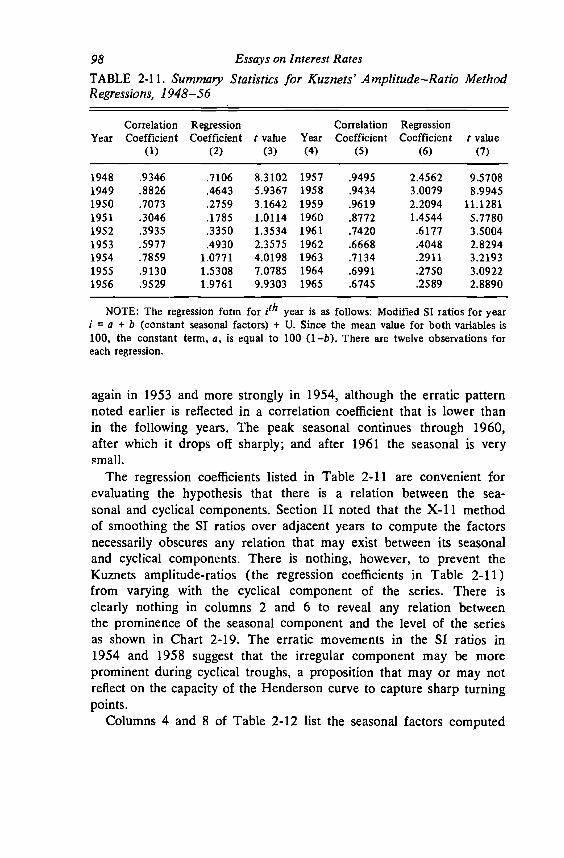
98 Essays on Interest RatesTABLE 2-11. Summary Statistics for Kuznets' Amplitude—Ratio MethodRegressions, 1948—56
YearCorrelationCoefficient
(1)
RegressionCoefficient
(2)t value
(3)Year(4)
CorrelationCoefficient
(5)
RegressionCoefficient
(6)t value
(7)
1948 .9346 .7106 8.3102 1957 .9495 2.4562 9.57081949 .8826 .4643 5.9367 1958 .9434 3.0079 8.99451950 .7073 .2759 3.1642 1959 .9619 2.2094 11.12811951 .3046 .1785 1.0114 1960 .8772 1.4544 5.77801952 .3935 .3350 1.3534 1961 .7420 .6177 3.50041953 .5977 .4930 2.3575 1962 .6668 .4048 2.82941954 .7859 1.0771 4.0198 1963 .7134 .2911 3.21931955 .9130 1.5308 7.0785 1964 .6991 .2750 3.09221956 .9529 1.9761 9.9303 1965 .6745 .2589 2.8890
NOTE: The regression form for year is as follows: Modified SI ratios for yearI = a + b (constant seasonal factors) + U. Since the mean value for both variables is100, the constant term, a, is equal to 100 (1—b). There are twelve observations foreach regression.
again in 1953 and more strongly in 1954, although the erratic patternnoted earlier is reflected in a correlation coefficient that is lower thanin the following years. The peak seasonal continues through 1960,after which it drops off sharply; and after 1961 the seasonal is verysmall.
The regression coefficients listed in Table 2-1 1 are convenient forevaluating the hypothesis that there is a relation between the sea-sonal and cyclical components. Section II noted that the X-1 1 methodof smoothing the SI ratios over adjacent years to compute the factorsnecessarily obscures any relation that may exist between its seasonaland cyclical components. There is nothing, however, to prevent theKuznets amplitude-ratios (the regression coefficients in Table 2-11)from varying with the cyclical component of the series. There isclearly nothing in columns 2 and 6 to reveal any relation betweenthe prominence of the seasonal component and the level of the seriesas shown in Chart 2-19. The erratic movements in the SI ratios in1954 and 1958 suggest that the irregular component may be moreprominent during cyclical troughs, a proposition that may or may notreflect on the capacity of the Henderson curve to capture sharp turningpoints.
Columns 4 and 8 of Table 2-12 list the seasonal factors computed

Seasonal Variation of Interest Rates 97
one may argue that seasonal analysis is concerned not with the rela-tion between climate and soft drink consumption but only withsystematic intrayear changes in consumption regardless of cause. Thispoint of view is predicated on the idea that seasonals are importantbecause they are predictable by mechanical projections of past be-havior; any variation that is not predictable in this way, even whenit is caused by the same variables that cause the predictable variation,is not seasonal. In cases, such as interest rates, where there areabrupt changes in the amplitude of seasonal, or, if you will, intrayear,variation, the choice of the appropriate adjustment depends on whichof the two concepts of a seasonal movement is intended.
To illustrate the practical significance of this issue the study ex-perimented with alternate adjustments of Treasury bill rates. TheKuznets amplitude-ratio method of adjustment is convenient for deal-ing with an abruptly changing seasonal amplitude provided the month-to-month pattern of factors is fixed, and only the amplitude changesfrom year to year. The factors are computed by regressing, one yearat a time, the twelve modified SI ratios42 on the set of constant factorsobtained by averaging, one month at a time, the modified SI ratiosover the whole period. The more similar the particular year's patternis to the average pattern the higher will be the correlation coefficient;when it is equal to one the regression coefficient will exactly measurethe proportionate difference in amplitude between them.43 Table 2-11lists the coefficients of correlation and regression, as well as thelatter's i-value, for the eighteen regressions from 1948 through 1965.All three statistics reveal the bell-shaped pattern in the seasonalamplitude that was noted earlier. Again, the seasonal in 1948 is un-usually clear, its pattern being highly correlated with the averagepattern. In the following two years the seasonal is still inexplicablystrong, although less than in 1948, the pegged prices notwithstanding.After two dormant years in 1951 and 1952, the seasonal emerges
That is, modified to eliminate extreme values. It is clearly important toeliminate the effect of extreme values on a regression computed with twelveobservations, although the X-1 1 modifications, used here, will in some casesdampen the very changes in amplitude the Kuznets method is designed to reveal.
In commenting on this method, Burns and Mitchell (op. cit., pp. 48—49)recommend not accepting the estimate when the correlation coefficient fallsbelow .7. It is clear that when the pattern changes, as in the case ofcommercial paper rates, the method has no value. The pattern for bill rates,however, is fairly stable; therefore, a low correlation coefficient signifies doubt-ful seasonality.

3.5
3.0
2.5
2.0
1.5 1.0 .54.5
4.0CH
AR
T 2—
19. O
rigin
al a
nd S
easo
nally
Adj
uste
d Se
ries o
f Tre
asur
y B
ill R
ates
, 194
8—65
Per
cent
5.0
I

Seasonal Variation of Interest Rates 95
the table includes the findings for all seventeen series considered inthis study.
Appendix: Alternate Adjustments of Treasury Bill RatesThere are several reasons for the differences between the curves ofSI ratios and seasonal factors in Charts 2-7 and 2-8. Most importantamong them is, of course, the seasonal factors' intended eliminationof the irregular component through its smoothing Out the nonrecurringvariation. One-time jumps, therefore, as in May 1960, appropriatelyresult in gaps between the two curves. It is easy to identify theseatypical (or irregular) jumps when they produce inversions (in thecase of May 1960 from a low to a high), but the identification is moredifficult when the atypical events exaggerate the usual fluctuationwithout seriously distorting the pattern. In 1958, for example, thetwo curves are far apart. There are no inversions, but the July troughis well below its value in adjacent years, and the October peak ishigh—both absolutely and relative to adjacent months. Short-terminterest rates were dropping sharply in the spring of 1958 (see Chart2-19), and investors, anticipating a continuing decline, borrowedheavily to purchase maturing Treasury bonds that earned rights to anew issue in June. Short-term capital gains on the new issue appearedcertain as all the indicators agreed the decline in rates would con-tinue. When short-term rates suddenly turned upward in June, theyleft many highly leveraged investors on the wrong end of the fulcrum.In addition to distorting the SI ratios, the resulting chaos invited acongressional investigation.4'
While it is easy and proper to shield the seasonal adjustment fromone-time changes in the pattern of SI ratios, it is much harder toapportion brief changes (whether lasting one or a few years) in theamplitude of a fixed pattern of SI ratios. There is no requirement thatthe seasonal amplitude be stable from year to year or even that itchange only gradually. For example, the seasonal in the consumptionof soft drinks is related to the weather; a particularly warm summerwill result in an atypically large seasonal amplitude. An adjustmentthat is constrained to gradual changes in amplitude will arbitrarilytruncate the seasonal amplitude in the above example. Alternatively,
41 Part of the results of this investigation are recorded in a fascinating studyof the crisis. See The Treasury-Federal Reserve Study of the GovernmentSecurities Market, Part II, Washington, D.C., February 1960.

94 Essays on Interest Ratesseasonal factors described for the short-term rates is less prominentin the case of long-term bonds, although the seasonal factors forsome of the series clearly evolve in this manner.
As in the other series considered in this study, there are some yearsfor which there appears to be no seasonal movement at all or forwhich, whether present or not, the seasonal is too small and uncertainto be measured. There is no accepted method for reliably choosingthe years for which an adjustment is appropriate. Nor do the neces-sary conditions prevail for reliable inference from the summarystatistics. Although there is a large subjective element involved in themethod used in this study, the primary criterion has been the apparentstability in the seasonal patterns regardless of their amplitudes. Butthe judgment involved in this study is restricted to the choice ofaccepting the results of the X-1 1 program. Additional judgment isrequired to improve this adjustment. Table 2-10 presents the sug-gested dates for accepting the machine adjustment. For convenience
TABLE 2-10. Suggested Periods for Accepting Seasonally Adjusted InterestRate Series
Series Period
Treasury bills 1948—659—12 month Treasury securities 1955—653—5 year Treasury securities 1955—59Long-term Treasury securities 1955—59Commercial paper rates 1956—63Bankers' acceptances 1948—63Industrial bondsa 1956—65Industrial bondsb 1950—65Public utility bondsa 1950—65Public utility bondsb 1951—61Corporate bondsa 1952—65Corporate bondsb 1952—65Railroad bondsa 195 3—63Railroad bondsb 1950—65Municipal bondsa 1950—65Municipal bonds1' 1950—65Municipal bondsc 1950—65
a Highest rating.bLowest rating.CHigh grade Standard and Poor.

CH
AR
T 2—
18 (c
oncl
uded
)
Inde
xIn
dex
90-
—11
0Lo
ng-t
erm
U. S
. bon
ds
110-
90C
orpo
rate
bon
ds, h
ighe
st r
atin
g
90-
—11
0C
orpo
rate
bon
ds, l
owes
t rat
ing
100
itO -
Mun
icip
al b
onds
, hig
hest
rat
ing
— g
o
90-
—11
0M
unic
ipal
bon
ds, l
owes
t rat
ing
100
II
9019
48'5
1'5
3'5
5'5
7'5
9'6
1'6
3'6
5

CH
AR
T 2—
18. S
easo
nal F
acto
rs fo
r Lon
g-Te
rm In
tere
st R
ates
, 194
8—65
Inde
xIn
dex
II
1I
II
110
-M
unic
ipal
bon
ds, h
igh
grad
e (S
tand
ard
& P
oor)
-
100
90In
dust
rial b
onds
,ra
ting
100
110
90lo
wes
t rat
ing
100 90
-hi
ghes
t rat
ing
100
90lo
wes
t rat
ing
100
90I
II
I
1948
'51
'53
'55
'57
'59
'61
'63
'65
'.0

Seasonal Variation of Interest Rates 91
CHART 2—17. SI Ratios and Seasonal Factors for Yields on CorporateBonds, Lowest Rating, One Month at a Time, 1948—65
sonality in these series throughout most of the sample period. Startingabout 1950, the seasonal factors are typically below the 100.0 line inthe first four months of the year, the trough usually occurring inMarch, rise above the line in midyear and beyond it to a peak inSeptember or October, then fall back to the 100.0 line in Novemberand December. Starting in 1955, the midyear months stay below the100.0 line, and the months at either end rise a little. The key sea-sonal months—March, April, September, and October—are largelyunaffected by this change. The prominent bell-shaped pattern in the
SI roliosSeasonal factors
Index
961948 '51 '53

1946
¶949
1952
______________
I I I I I 1 .111 1
F MAM J .J As 0 ND
Summary of Long-Term Bonds
In spite of the low seasonal amplitudes in long-term bonds, boththe summary statistics and the diagrams confirm the presence of sea-
90 Essays on Interest RatesCHART 2—16. SI Ratios and Seasonal Factors for Yields on CorporateBonds, Lowest Rating, 1948—65
SI ratiosSeasonal factors
Index Index Index Index105 105
100
95
105
100
95
105
100
95
.105
a
105
100
95
105
100
95
105
100
95
1954 ---
105951955
-
105 -
1956100
100
95
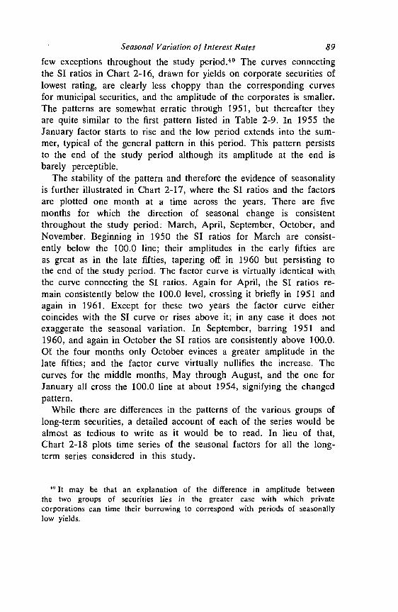
Seasonal Variation of Interest Rates 89
few exceptions throughout the study period.40 The curves connectingthe SI ratios in Chart 2-16, drawn for yields on corporate securities oflowest rating, are clearly less choppy than the corresponding curvesfor municipal securities, and the amplitude of the corporates is smaller.The patterns are somewhat erratic through 1951, but thereafter theyare quite similar to the first pattern listed in Table 2-9. In 1955 theJanuary factor starts to rise and the low period extends into the sum-mer, typical of the general pattern in this period. This pattern persiststo the end of the study period although its amplitude at the end isbarely perceptible.
The stability of the pattern and therefore the evidence of seasonalityis further illustrated in Chart 2-17, where the SI ratios and the factorsare plotted one month at a time across the years. There are fivemonths for which the direction of seasonal change is consistentthroughout the study period: March, April, September, October, andNovember. Beginning in 1950 the SI ratios for March are consist-ently below the 100.0 line; their amplitudes in the early fifties areas great as in the late fifties, tapering off in 1960 but persisting tothe end of the study period. The factor curve is virtually identical withthe curve connecting the SI ratios. Again for April, the SI ratios re-main consistently below the 100.0 level, crossing it briefly in 1951 andagain in 1961. Except for these two years the factor curve eithercoincides with the SI curve or rises above it; in any case it does notexaggerate the seasonal variation. In September, barring 1951 and1960, and again in October the SI ratios are consistently above 100.0.Of the four months only October evinces a greater amplitude in thelate fifties; and the factor curve virtually nullifies the increase. Thecurves for the middle months, May through August, and the one forJanuary all cross the 100.0 line at about 1954, signifying the changedpattern.
While there are differences in the patterns of the various groups oflong-term securities, a detailed account of each of the series would bealmost as tedious to write as it would be to read. In lieu of that,Chart 2-18 plots time series of the seasonal factors for all the long-term series considered in this study.
'° It may be that an explanation of the difference in amplitude betweenthe two groups of securities lies in the greater ease with which privatecorporations can time their borrowing to correspond with periods of seasonallylow yields.
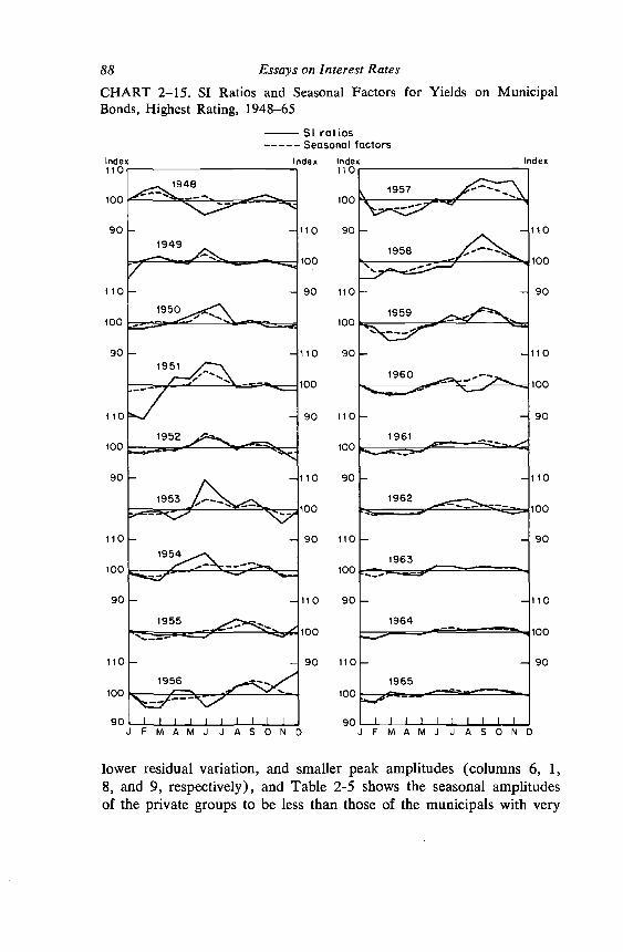
1951
-110
- 110
1 — _j_ 100
Index
1957
- -110
- -110
100
- -901961
— -
- - 110
1962
— - 90
1963
- 110
1964
- 901965
I I I I I I I I I I
J F MAMJ JASON D
lower residual variation, and smaller peak amplitudes (columns 6, 1,8, and 9, respectively), and Table 2-5 shows the seasonal amplitudesof the private groups to be less than those of the municipals with very
88 Essays on Interest RatesCHART 2—15. SI Ratios and Seasonal Factors for Yields on MunicipalBonds, Highest Rating, 1948—65
SI ratLosSeasonal factors
Index Index Index110 110
1948
90
110
100
1949110
109
90
90 - -110
I
110
100
90
110
100
90
100
90
110
100
90
ItO
100
90
110
100
90
110
100
90
110 -
100
90
901956
I IJ FMAMJ J ASOND

Seasonal Variation of Interest Rates 87MUNICIPAL SECURITIES. Of all the long-term securities, the F statisticsare among the lowest and the amplitudes among the highest for theyields on the three municipal bond series considered. The F statistics,however, are not brought down, as in the case of long-term Trea-suries, by constantly shifting patterns of small amplitude and erratictransition periods; nor is the F statistic spuriously high as a result ofthe attenuation of the peak seasonal in the late fifties. Chart 2-15 plotsthe seasonal factors and SI ratios for yields on municipal bonds ofhighest rating. Excluding the first two years, the pattern in the earlyyears is quite similar to the general pattern of this period describedin Table 2-9: lows during the first four months, a June peak, but then,unlike the general pattern, a rapid decline to lows in the last twomonths. The large gaps between the curves, implied in the unusuallylarge irregular component recorded in column 1 of Table 2-4, reflectchanges in the seasonal amplitude of the series rather than an un-stable pattern. Although the greater dispersion of a given month's SIratios results in less reliable estimates of the seasonal factors, thediagrams reveal the SI ratios for given months to fluctuate aboutmeans that clearly remain above or remain below the 100.0 line.From 1949 through 1954, every June is a high, and every Januaryand December are lows. In 1955 the new pattern emerges, againsimilar to the general pattern of the late fifties, with a trough inFebruary or March and a peak in September. The pattern changessomewhat after 1959, but persists in similar form through the endof the study period.
In this case, therefore, and in the case of the other municipal groupsnot shown here, a basis for seasonal adjustment exists in spite of thefeeble F statistics. There is an important difference between the ef-fects of random variations in seasonal amplitude and those in theseasonal pattern on identifying the presence of seasonality. In theformer case, by narrowly defining extreme points, the program candampen the estimated seasonal amplitudes, imposing a downwardbias on the estimated means, and thereby reducing the risk of wronglyaffirming the presence of seasonality. In the latter case, the danger isgreater that the program will impose a seasonal pattern on the series.
PRIVATE LONG-TERM SECURITIES. Although there are differences indetail it is convenient to describe the seasonality of yields on privatelong-term securities for the group as a whole. This group's seasonalpattern differs from that of the municipals by its somewhat smalleramplitude and its greater stability. Table 2-4 records higher F statistics,

Seasonal Variation of Interest Rates 121
in supply, on the other hand, are subject to the discretion of the au-thorities. An estimate of the demand for short-term credit, therefore,is available from successive observations of the rate of interest neces-sary for people to hold the amount of money that is offered. Morespecifically, the analysis reveals the seasonal shift in the interest ratenecessary for people to accept the seasonal shift in supply of money,given their fixed seasonal shift in demand.68 The only fixity in thishypothetical system is in the demand for short-term credit; the interestrate varies as the supply varies—hence, the moving seasonal in in-terest rates.
The immediate purpose of this study is not to estimate the demandfor short-term credit for its own sake, but rather to investigate thecauses of the changing seasonal amplitudes (i.e., from year to year)of the interest rates. Given the above analysis, the first step would beto regress the seasonal factors of Treasury bills on those of moneysupply, one month at a time across years. In other words, regress theJanuary factor for bill rates on the January factor for money supplyin 1948, 1949, . . . , 1965: eighteen observations in each of twelveregressions. The regression coefficients, their t values, and the adjustedcoefficients of determination are listed in Table 2-16. While the resultsare far from conclusive, in the five cases where the regression co-efficients are statistically significant they reveal the expected inverserelation between the demand for money and the interest rate.
While the assumed stability in the seasonal demand for credit isplausible in the case of private demand, the government may haveoccasion to vary its demand both to meet changing fiscal requirementsand, where possible, to take advantage of any seasonal in interestrates that may occur. Introduction of this factor, in the form of varia-tion of total bills outstanding, leads to a considerable improvementin the estimates. The results, analogous to those in Table 2-16 butwith the addition of total bills outstanding, are shown in Table 2-17.Eight instead of five of the money supply coefficients are significant,and each of the eight is negative. Eight of the coefficients of billsoutstanding are positive, and six of these are significant. That is, in
The terminology used here, admittedly awkward, does not imply that thedemand is for money to hold as an asset; a demand for which there is noobvious reason for a seasonal increase in the autumn. In the present contextthe "demand for money" is only an abstraction that may help explain the in-verse correlation between the seasonal amplitudes of money supply and Trea-sury bill rates. This point.is considered in greater detail in the appendix to thissection.

122 Essays on interest Razes
TABLE 2-16. Regression of Seasonal Factors of Treasury Bill Rates onThose of Money Supply, 1948—65
M 2
January 3.9474 .8381 a
February —9.4012 .69622March 1.4503 .4107 a
AprilMay
—.9290—9.2617
—.8665—2.027&'
a
.15460June —4.4874 —1.6004 .08412July 14.3076 .9028 a
August .0644 .0279 a
SeptemberOctober
.6536—20.6351
1.3084—4.047 2b
.04020
.47498November —23.4467 .16545December —8.4171 . .16545
NOTE: Each of the twelve regressions is specified as follows: seasonal factor (billrate) = a + b [seasonal factor (money supply)1 +E. Each regression is run witheighteen observations.
aThe estimated adjusted coefficients of determination are negative.bStatistically significant at the 5 per cent level.
TABLE 2-17. Regression of Seasonal Factors of Treasury Bill Rates onThose of Money Supply and Total Bills Outstanding, 1 948—65
Month bMoN t bT0T t R2(adj)
January —7.8027 2.4944 6•8616a .73768February —12.6356 —.6275 .87787March .1628 .0468 1.5159 1.5604 .03512April —7.7407 6.7563 5•5998a .64973May —9.9774 —1.7788 —.3225 —.2443 .10181June —9.0975 1.3450 55671a .68138July 18.7018 1.0639 —.8688 —.6337 —.05029August —12.1313 3.2720 .35756September .7938 1.7885 —1.2068 .25581October —25.5305 1.8186 1.7840 .53800November ..393554 10.4859 47151a .64137December —2.6776 3.8698 .96636
NOTE: Each of the twelve regressions is specified, as follows: seasonal factor (billrate) = a + b1 [seasonal factor (money supply)] + b2 [seasonal factor (total billsoutstanding)] + E. Each regression is run with eighteen observations.
aStatistically significant at the 5 per cent level.

Seasonal Variation of Interest Rates 123
most, but not all, cases where the coefficients are statistically signifi-cant they have the expected sign: Increases in the money supply re-duce the bill rate; while increases in bills outstanding increase the billrate.
To obtain these results it is obviously necessary to run the regressionsone month at a time across the years (or to use the equivalent dummyvariable technique described below) since the month-to-month changesin the seasonal factors of Treasury bill rates and money supply havevirtually the same directions and are positively correlated. During .acyclical upturn both the demand for money and the supply of moneyincrease, but since the demand increases faster than the supply, theinterest rate increases as well. In this situation, an increase in thesupply of money coincides with an increase in interest rates, and thecareless observer sees a positively sloped demand curve. Similarly,over the course of the year the demand for money changes in thesame direction as the supply but faster, so that the interest rate variesin the same direction as the supply. However, working with deviationsfrom the trend-cycle component isolates the common cyclical componentin the demand and the supply; and estimating the relation between in-terest rates and money supply for one month at a time in effect exploitsthe relative constancy in the seasonal shifts in demand. It is then feasibleto measure the points of intersection between the fixed demand curveand the varying supply curve and, therefore, to estimate the elasticityof demand with respect to the interest rate.
Instead of estimating twelve separate regressions (one for eachmonth) of the seasonal factors for Treasury bill rates on those ofthe money supply and the total number of bills outstanding, it ispreferable to pool all the observations and isolate the intrayear, month-to-month movements by means of dummy variables. Table 2-18 liststhe results of this regression estimated both ways, with and withoutdummy variables. In regression A, without dummy variables, the com-mon seasonal patterns dominate the relation between the seasonalfactors of Treasury bill rates and, money supply, and thus the regres-sion coefficient is positive. In terms of the schematic representation,both the demand and the supply curves vary'S together, the demandvarying more than the supply; therefore, the interest rate varies withthe supply. An analogous result is frequently observed in the positivecorrelation between interest rates and money supply over the businesscycle when no allowance is made for the joint movement of supplyand demand.
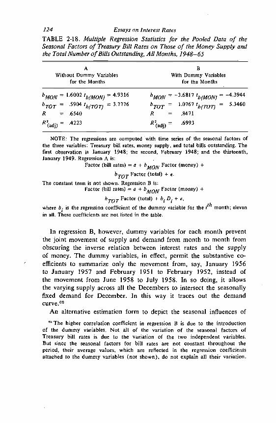
124 Essays on interest RatesTABLE 2-18. Multiple Regression Statistics for the Pooled Data of theSeasonal Factors of Treasury Bill Rates on Those of the Money Supply andthe Total Number of Bills Outstanding, All Months, 1948—65
AWithout Dummy Variables
for the Months
BWith Dummy Variab
for the Monthsles
bMON 1.6002 tb(MON) = 4.93 16 bMON = —3.6817 tb(MON)
bTQT = .5904 tb(TOT) = 3.7776 bTOT = 1.0767 tb(TOT) = 5.3460
R = .6540 R = .8471
R2(adj) — .4223 R2(adj) = .6993
NOTE: The regressions are computed 'with time series of the seasonal factors ofthe three variables: Treasury bill rates, money supply, and total bills outstanding. Thefirst observation is January 1948; the second, February 1948; and the thirteenth,January 1949. Regression A is:
Factor (bill rates) = a + bMON Factor (money) +
bror Factor (total) + e.
The constant term is not shown. Regression B is:Factor (bill rates) = a + bMON Factor (money) +
Factor (total) + b, D, + e,
where b1 is the regression coefficient of the dummy variable for the 1th month; elevenin all. These coefficients are not listed in the table.
In regression B, however, dummy variables for each month preventthe joint movement of supply and demand from month to month fromobscuring the inverse relation between interest rates and the supplyof money. The dummy variables, in effect, permit the substantive co-efficients to summarize only the movement from, say, January 1956to January 1957 and February 1951 to February 1952, instead ofthe movement from June 1958 to July 1958. In so doing, it allowsthe varying supply across all the Decembers to intersect the seasonallyfixed demand for December. In this way it traces out the demandcurve.00
An alternative estimation form to depict the seasonal influences ofThe higher correlation coefficient in regression B is due to the introduction
of the dummy variables. Not all of the variation of the seasonal factors ofTreasury bill rates is due to the variation of the two independent variables.But since the seasonal factors for bill rates are not constant throughout theperiod, their average values, which are reflected in the regression coefficientsattached to the dummy variables (not shown), do not explain all their variation.
Seasonal Variation of Interest Rates 125
money supply and government borrowing makes use of the variancesof the seasonal factors described in Section I. The variance of themonthly factors, computed for each year,- measures the amplitude ofthe seasonal factors. Regressing the variance of Treasury bill ratefactors (eighteen observations) on the variance of money supply andtotal bills outstanding factors reveals the inverse and direct relation-ships, respectively, of the seasonal influence of these two series onthe bill rate seasonal. The results of the regression are recorded inTable 2-19.
TABLE 2-19. Multiple Regression Statistics for the Variance of the SeasonalFactors of Treasury Bill Rates on Those of Money Supply and Total BillsOutstanding, 1948—65
PartialVariable b tb Constant Correlation R R2(adj)
Moneysupply —75.1311 —5.1253 —.7978Total bill 114.4613 .8969 .7783Outstanding 6.7873 6.8102 .8693
NOTE: The regressions are computed with time series of the variances of themonthly seasonal factors for each series. For a given year and series the variance iscomputed for the twelve factors from January through December. Since the meanfactor is 1, a greater seasonal amplitude implies a greater dispersion around the meanand hence a greater variance. The form of the regression is:
Var. (fact. bill rates) = CONST. ± bMON Var (fact. money supply)Var (fact. bills outstanding) + residual.
It is of course not possible to distinguish intentional changes inthe seasonal variation of government borrowing to take advantageof the seasonal in interest rates from the unintentional responses toseasonal fiscal The Treasury's ability to adjust thetiming of its offerings to benefit from seasonal lows in interest ratesis not unlimited, it is pointless to borrow merely because the rate islow. The problem here is analogous to the arbitrage issue discussedearlier in this section.
In the case of the money supply, the Federal Reserve was merely assumedto have discretion over the supply. To the extent this assumption is unwar-ranted the distinction discussed in the text applies to the money supply as well.However, arguments against Federal Reserve control of the money supplyrely to a large extent on the variability of time deposits, which, in the absenceof a seasonal, are not germane to the present discussion.

126 Essays on Interest RatesFrom the above analysis it is a small step to compute the actual
elasticity of demand for money with respect to the short-term interestrate. To do this, the variables in regression B of Table 2-18 havesimply been rearranged.7' Now the seasonal factors for money supplyform the dependent variable, and the seasonal factors for Treasurybill rates form one of the independent variables. Since these variablesare already expressed as percentages of the moving average, the re-gression coefficients signify elasticities. The elasticity of demand forshort-term credit with respect to the short-term interest rate accordingto this method of estimation is —.023 7 (Table 2-20). The puninessTABLE 2-20. Multiple Regression Statistics for the Pooled Data of theSeasonal Factors for Money Supply on Those of Treasury Bill Rates andTotal Bills Outstanding, All Months, 1 948—65
bb,ll = —.0237 tb(bill) = —4.3944
bTot = .0884 tb(Tot) = 5.4861R = 9849a
= 9681a
NOTE: The regression is computed as follows:Factor (money) = a + Factor (bill rate) +
Factor (total) + b3 D, + e,
where Factor (money) is the seasonal factors of money supply; Factor (b ill rate) is theseasonal factors of Treasury bill rates; Factor (total) is the seasonal factors of totalbills outstanding; and is the regression coefficient of dummy variable for month.
aThe correlation coefficient is very high because the dummy variables explain alarge part of the seasonal variation of money supply. The strength of this relationshipis due to the relative stability of the seasonal factors of money supply and theirsusceptibility, therefore, to the dummy variable technique for seasonal adjustment.(This point is considered in Section II.)
of the estimated elasticity by no means implies its economic insignifi-cance. On the contrary, it implies that a relatively small change inmoney supply may have a relatively large short run impact on interestrates. Chart 2-22 foreshadowed this result in the association it showedbetween the relatively small changes in the seasonal amplitude of money•and the relatively large changes in the opposite direction of the sea-sonal amplitude of Treasury bill rates.
The pooled data were used for this experiment since the regression co-efficients computed with the variance data are further removed from the conceptof elasticity.

Seasonal Variation of Interest Rates 127
Interpretation of this result, however, must take account of an im-portant limitation of the estimation procedure used. By definition theseasonal factors for a given month are serially correlated, one yearwith the next. If the factor is high in December 1952, it will be highin December 1953 as well. This serial correlation in the observationsseverely limits the actual degrees of freedom as distinct from the nomi-nal amount. In effect, the seasonal amplitude of Treasury bill ratesis low, then high, then low; and that of the money stock high, thenlow, then high. In addition to these three points, there are smallerchanges in between, especially with respect to the variation of theseveral months; but the total is not even near the nominal 202 degreesof freedom.72 The uncertain degrees of freedom reduces the impor-tance of the estimated test of significance of the estimated elasticities.The figures are therefore less reliable estimates, although there is noreason for thinking them biased. In any case, the relatiàns describedconstitute an hypothesis that further work can corroborate or refute.
Conclusions
This section reached the following conclusions:(1) .A seasonal variation in long-term bonds can survive arbitrage
so long as the amplitude does not exceed some specified amount.This amount will be greater the more important is the irregular com-ponent of the series, the shorter is the maturity of the bond, andthe greater is the margin requirement for borrowing money to pur-chase bonds. There are, no doubt, other factors that this section didnot consider.
(2) The analogous computation for short-term securities is com-plicated by the term structure of interest rates. Other things being thesame, the seasonal amplitude for a given year will be greater, thegreater is the slope of the yield curve. Since the yield curve is typicallysteepest when the level of rates is low, the seasonal amplitude on thisaccount should be greatest when the level of rates is low. This con-sideration is apparently offset by the higher borrowing costs to ar-bitrageurs, when the level of rates is high.
72 The number is computed as follows: 12 months in each of 18 years comesto 216. There are .2 independent variables, a constant term, and 11 dummyvariables. 216 — 14 202. Substitution of the SI ratios for the factors will notsolve this problem (though it would reduce it) because the presence of sea-sonality implies the serial correlation of the SI ratios.

128 Essays on Interest Rates
(3) The variation in the seasonal amplitude of the Treasury billrate is closely related to the movement of the seasonal amplitudesof money supply and total bills outstanding. These relationships dem-onstrate the influence over the seasonal in the Treasury bill rate en-joyed by the Federal Reserve and the U.S. Treasury.
(4) There is an inverse relationship between the seasonal amplitudeof Treasury bill rates and that of money stock. This relationship im-plies a negatively sloped demand curve for money with respect tointerest rates. The elasticity of this curve is very small.
Appendix
There are at least three interpretations of what the text calls the esti-mated elasticity of demand for money with respect to interest rates:the slope in the observed regression of the logarithms of money supplyon interest rates; the elasticity with respect to interest rates of thedemand for money to hold as an asset; and the elasticity with respectto interest rates of the demand for loanable funds.
The first simply describes an observed association and is noncon-troversial. The second implies the interest rate is one determinant ofthe demand for money-as-an-asset. However, there is no reason fora seasonal in this demand; and since the method used to estimatethe elasticity assumes a seasonal shift in demand, this interpretationis not appropriate. The third assumes that the only seasonally opera-tive component of the change in the supply of loanable funds is thesupply of new money so that, given the demand for loanable funds,the shift in supply due to the change in money supply would determinethe interest rate. But with a lower interest rate the demand for money-as-an-asset would rise and offset—partially, totally, or more thanoffset, depending on the relevant elasticities—the new money com-ponent of loanable funds. Therefore, according to the third interpre-tation the estimate of the elasticity of demand for loanable funds isbiased downward (in absolute magnitude) because the change in loan-able funds is lcss than the change in money supply.
This problem is only one illustration of the difficulty in specifyingthe conditions for which a demand curve is drawn. As already noted,the method used here avoids the problem of a cyclical componentcommon to both the supply of and demand for money. Its referenceto month-to-month variation probably alleviates other difficulties en-
Seasonal Variation of Interest Rates 129
countered in demand studies.73 Its short-term character obviates con-sideration of the effect of additional supplies of money combined withlower interest rates on nominal income and, through income, the in-creased demand for money for transactions purposes. Depending onthe relevant elasticities and periods of adjustment, additional moneycould conceivably raise rather than lower the interest rate by increas-ing the demand for money both as an asset and as a medium of ex-change. With the increased income the demand for loanable fundswould rise. All these effects could offset the effect on interest ratesof the increased supply of money. In addition, the short run analysisobviates consideration of the effect of a change in interest rates onthe proportion of income that is saved, which would, in turn, affectthe supply of loanable funds. For the same reason any effect of thechange in money supply on the price level and, through this effect,on interest rates is also outside the scope of this analysis.
These points have in common the difficulty of holding constantnominal (or real) income, fixing the demand curve for money whilethe supply of money is allowed to vary. Variation in money supplyimplies variation in income and that, in turn, implies shifts in thedemand curve for money. The relationship among the three—moneysupply, income, and demand for money—is stronger the greater isthe period allowed for adjustment. Choosing coeval observations ofthe relevant variables that span brief periods (months, for example,instead of years) limits the process of diffusion of the new moneysupply and alleviates the identification problem. To the extent, how-ever, that the diffusion process is anticipated in the market, as, forexample, when increases in money supply are taken to forebode in-flation, estimated parameters based on short-period observations willsuffer from the identification problem.
These problems in demand analysis are by no means peculiar to thisstudy nor even to analyses of the demand for money, although theubiquity of money may aggravate the problems of demand analysis.Ultimately, one is sure only of the first interpretation, namely, thatthe estimated parameters described an observed association. Depend-ing on how the problem is set up—how the demand curve is specified,what is the source of the observations and their time dimension—andwhat relationship among the variables is assumed, the writer can infer
Some of these difficulties are noted by Milton Friedman and Anna Jacob-son Schwartz in Monetary Statistics of the United States: Estimates, Sources,Methods, New York, NBER, 1970.

130 Essays on Interest Rates
behavioral parameters from the observed association. It is then hisresponsibility to justify the inferences.
V. SUMMARY AND CONCLUSIONS
There is compelling evidence of the presence of repetitive seasonalmovements in both long- and short-term interest rates in the yearsbetween 1955 and 1960. Outside this period, both before and after,the evidence is less conclusive, and certainly the seasonal movementsare smaller. Nevertheless, a seasonal pattern apparently existed inmost of the rates studied over a period substantially longer than thebrief period of peak seasonality. This result is largely predicated onthe demonstrated similarities among the seasonal patterns of the sev-eral rates, as well as the relative uniformity of the pattern for a givenrate over an extended period. The study's primary focus is on thequality of the evidence for these conclusions.
The seasonal factors for short-term rates are found typically todecline from a relative high in January through the spring months toa trough in June and then sharply increase to September, from whichthey rise gradually to a peak in December. This pattern is conspicuousin the late fifties but occurs with some variation throughout the post-war period. The amplitudes, however, vary considerably, rising graduallyafter the early fifties through 1957 or 1958 and falling off quiterapidly thereafter. By 1965 the seasonal movement had all but van-ished, although recent evidence not considered in this study indicatessome resurgence in the seasonal.
The seasonal pattern for yields on bankers' acceptances is, perhaps,the most stable of those examined, although its amplitude is some-what less than that of Treasury bill rates. During part of the period ofpeak seasonality, the amplitudes, that is, the variation from seasonalhigh to seasonal low, exceeded 20 per cent of the level of the series.These amplitudes dropped sharply after 1959. By 1963, the seasonalpattern for bankers' acceptances virtually disappeared. The seasonalpattern for Treasury bills appears to have continued through 1965,the end of the study period, although its amplitude then was barely 2per cent of the level of the series. The seasonal movement in com-mercial paper rates is far less stable and its amplitude smaller thanthose of the other two series.
While this study did not specifically evaluate the relation betweenseasonal amplitude and term to maturity, there is an obvious declinein both seasonal amplitude and the period over which there is a
Seasonal Variation of Interest Rates 131
measurable seasonal factor, as the maturity of Treasury securities in-creases. The patterns of the seasonal factors of long-term rates areless stable than those of the short-term rates (except commercialpaper) and have a much smaller amplitude. In the early fifties thepattern typically starts with a January low that falls to a trough inMarch, then rises to a plateau extending from June to October,before declining to an intermediate position for the last two months.The patterns for all the private long-term bonds are alike with respectto their midyear highs and January lows, the characteristic distinguish-ing these patterns from those of the same securities in the laterperiod, as well as from the patterns of the short-term rates. Startingin 1955 the seasonal patterns of private long-term bond rateschange—the January factors from lows to highs and the June andJuly factors from highs to lows. The troughs remain in March andApril and the peaks in September and October. As in the case ofthe short-term rates the amplitude is greatest in the late fifties andtapers off thereafter. By 1965, the amplitude is very low and in somecases nonexistent.
While this evidence strongly supports the view that seasonalityexists in the interest rate series, questions relating to the methods, aswell as the desirability of adjusting the data for seasonal variations,remain. In addition to the sampling problem of drawing from ahypothetically stable population (a common problem of empiricaleconomics), the estimation of seasonal factors must cope with theeffects of a shifting population. That is, the seasonal factors for agiven month estimated for different years differ not merely becauseof random fluctuations but also because the true value, apart fromrandomness, may itself be varying. The difficulty in empirical seasonalanalysis is to distinguish the random from the systematic variation ofthe seasonal factors. While it is possible to devise tests of the sig-nilicance of differences in estimated factors for nonoverlapping periods,a continuous reading of their accuracy from year to year is elusive.Visual comparisons of the adjusted with the nonadjusted data (or,correspondingly, the seasonal factors with the ratios-to-moving-aver-age) may help to determine whether the estimated seasonal com-ponent captures the systematic seasonal movements of the raw data.Unfortunately, this method ties the conclusions to the particularanalyst and invites differences in judgment. Because of the subjectivityof this element, the study merely suggests the periods within whichthe factors are deemed relatively accurate.

132 Essays on interest RatesWhile the similarity in the patterns of all the long-term rates con-
sidered is strong evidence of a seasonal element in the rates, thepatterns themselves may not be sufficiently stable to warrant an at-tempt to eliminate this element. The question whether a seasonalpattern exists is distinct from the question whether the seasonal move-ment is sufficiently stable to justify seasonally adjusting the dataand risking the introduction rather than the elimination of variation.It is often maintained that a seasonal pattern in long-term rates wouldnot persist because of the profits available to those who would ar-bitrage the seasonality away by buying securities in periods of sea-sonally high rates and selling them when the rates are seasonally low.This argument is true only to the extent the seasonal amplitude is suf-ficient to cover the costs of arbitrage, including the risk that onany given occasion the cyclical, trend, or random components mayswamp the seasonal effect, and to the extent the seasonal movementis sufficiently stable to make the arbitrage more than a mere specula-tion. The greater the importance of these two effects—swamping byother components of variation and instability from year to year—thegreater will be the seasonal amplitude that will survive arbitrage.Municipal bond yields, for example, a series with a large irregularcomponent and an unstable seasonal component, has a relatively highseasonal amplitude.
The cause of the variation in seasonal amplitudes, the salientcharacteristic of the seasonals observed in this study, is a complexissue. At the risk of oversimplification this study considered theproblem in the light of the supply of and demand for money. On theassumption that the seasonal variation in the demand for money isrelatively constant from year to year, the change from year to yearin the seasonal patterns for short-term interest rates would depend onthat of the seasonal patterns for the supply of money. In years whenthe seasonal factor for, say, January in money outstanding is highthe corresponding seasonal factor for interest rates would be low; andwhen the former is low the latter would be high. The observed rela-tionship between the changing seasonal factors of money supply andshort period interest rates is, indeed, inverse. Hence, the data areconsistent with the hypothesis that the rise in the amplitude of theseasonal variations in interest rates during the 1950's and its virtualdisappearance during the 1960's is attributable to changes (in theopposite direction) in the seasonal movements in money supply. Thisinverse relationship is more conspicuous when allowance is made

Seasonal Variation of Interest Rates 133
for seasonal movements in the quantity of bills outstanding, a findingconsistent with the hypothesis that the Treasury made some attemptto benefit from the seasonal variation in interest rates. Failure totake account of this effect, which involves a change in demand inthe same direction as the change in supply, obscures the relationbetween money supply and interest rates. When this change in de-mand is statistically nullified the full effect of the change in supplyis observable.