the sedimentation of colloidal nanoparticles in solution
TRANSCRIPT

HAL Id: hal-01637907https://hal.archives-ouvertes.fr/hal-01637907
Submitted on 18 Nov 2017
HAL is a multi-disciplinary open accessarchive for the deposit and dissemination of sci-entific research documents, whether they are pub-lished or not. The documents may come fromteaching and research institutions in France orabroad, or from public or private research centers.
L’archive ouverte pluridisciplinaire HAL, estdestinée au dépôt et à la diffusion de documentsscientifiques de niveau recherche, publiés ou non,émanant des établissements d’enseignement et derecherche français ou étrangers, des laboratoirespublics ou privés.
The sedimentation of colloidal nanoparticles in solutionand its study using quantitative digital photography
Johanna Midelet, Afaf El-Sagheer, Tom Brown, Antonios Kanaras, MartinusH. V. Werts
To cite this version:Johanna Midelet, Afaf El-Sagheer, Tom Brown, Antonios Kanaras, Martinus H. V. Werts. Thesedimentation of colloidal nanoparticles in solution and its study using quantitative digital photogra-phy. Particle and Particle Systems Characterization, Wiley-VCH Verlag, 2017, 34 (10), pp.1700095.�10.1002/ppsc.201700095�. �hal-01637907�

The sedimentation of colloidal nanoparticles insolution and its study using quantitative
digital photography
Johanna Midelet1, Afaf H. El-Sagheer2, Tom Brown2,Antonios G. Kanaras1, and Martinus H. V. Werts*3
1University of Southampton, Physics and Astronomy, Facultyof Physical Sciences and Engineering, Southampton SO171BJ,
U.K.2University of Oxford, Department of Chemistry, 12 Mansfield
Road, Oxford, OX1 3TA, U.K.3Ecole normale superieure de Rennes, CNRS, lab. SATIE,
Campus de Ker Lann, F-35170 Bruz, France
author version, accepted manuscript published asPart. Part. Syst. Charact. 2017, 1700095
DOI: 10.1002/ppsc201700095
Abstract
Sedimentation and diffusion are important aspects of the behaviourof colloidal nanoparticles in solution, and merit attention during thesynthesis, characterisation and application of nanoparticles. Here westudy the sedimentation of nanoparticles quantitatively using digitalphotography and a simple model based on the Mason-Weaver equa-tion. Good agreement between experimental time-lapse photographyand numerical solutions of the model was found for a series of goldnanoparticles. The new method was extended to study for the firsttime the gravitational sedimentation of DNA-linked gold nanoparticledimers as a model system of a higher complexity structure. Addition-ally we derive simple formulas for estimating suitable parameters forthe preparative centrifugation of nanoparticle solutions.
1

1 Introduction
Observations on the sedimentation of colloidal solutions were important his-torically in establishing the physical reality of molecules and providing amolecular basis for thermodynamics in the form of statistical mechanics.[1–3] Nowadays, there is an intense interest in the development of colloidalsolutions of engineered nanocrystals for a variety of applications. These so-lutions should display sedimentation behaviour in line with expectations forthese particles on basis of their shape, composition and suspending medium.
For stable and dilute solutions of sufficiently large particles, the sedimen-tation behaviour (Figure 1) is a result of the particular interplay of nanopar-ticle hydrodynamics, and gravitational and Brownian forces. Under theseconditions, the surface chemistry of the nanoparticles, while ensuring col-loidal stability, does not significantly influence the sedimentation behaviour.For smaller particles (< 10 nm), and in particular ’soft’ particles such aspolymers and proteins, solvation effects on sedimentation may become sig-nificant, as the shell of solvent molecules around the object influences itshydrodynamic behaviour.[4–6] Furthermore, the presence of surfactants in-teracting with colloidal particles may change sedimentation behaviour[7, 8].These effects are not considered in the present work.
A general understanding of the sedimentation of nanoparticle solutionsis useful as it may give rapid and visual clues about the size distributionand colloidal stability of newly synthesised colloids. These clues go beyondthe simple assessment of whether a prepared solution is colloidally stable.Careful monitoring of sedimentation behaviour may be used to verify thenature of the suspended object in its native medium, and is complemen-tary to methods that characterise a limited number of specimens depositedon a substrate, such as electron microsopy. Furthermore, sedimentation,decantation and controlled centrifugation are often purification steps in wet-chemical synthesis of nanoparticles and nanoparticle assemblies, for instancefor the purification of gold nanorods.[9] A further example is the purifica-tion of nanoparticles by flocculation and subsequent sedimentation. Floc-culation under the influence of depletion forces due to specific flocculatantsproduces large aggregates of these nanoparticles that settle rapidly leavingnon-flocculated impurities in the supernatant.[10–12].
When analysing the interaction of nanoparticles with biological systemsin therapeutic and diagnostic applications, their transport properties such asdiffusion and sedimentation need to be taken into account The importanceof sedimentation to in vitro studies of cellular uptake of nanoparticles hasbeen demonstrated.[13]
There is a clear connection between the gravitational sedimentation of
2

Figure 1 – Sedimentation versus Brownian diffusion in colloidal solutions. (a)Gravity tends to direct dense particles to the bottom of the cell, whereas therandom Brownian forces tend to disperse the particles throughout the entirevolume. (b) This leads to the establishment of an equilibrium gradient start-ing from an initial homogeneous distribution of particles. Here we trace thetheoretical initial, transient and equilibrium concentration profiles as a func-tion of vertical position. (c) Experimental observation of sedimentation overtime of colloidal gold (20, 40, 60 nm) in water using quantitative digital pho-tography. The cell at the left of each picture contains water only. Photos weretaken at the start, and after 7, 14 and 35 days, respectively. The rightmostpicture represents the cells at equilibrium: a photograph of the Boltzmanndistribution.
colloidal particles and analytical centrifugation techniques, where sedimen-tation is sped up by increasing g to multiples of the earth gravitationalpull. Analytical ultracentrifugation (AUC), which is well known for itsapplications in biochemistry, has been successfully applied to the study ofnanoparticle solutions.[14–17] Optimisation of the measurement using a spec-troscopic approach in combination with detailed numerical analysis of themulti-wavelength sedimentation profiles has made AUC extremely versatilefor the analysis of nanoparticle preparations.[18] It has furthermore beendemonstrated that information on the shapes of DNA-based nanoparticle as-semblies can also be obtained for AUC sedimentation analysis combined withhydrodynamic modeling.[19]
The rotational speed and centrifugal acceleration in analytical ultracen-trifuges are extremely high, and adapted to proteins and small bioparti-cles. As will be further pointed out later on, many assemblies of inorganicnanoparticles, which have higher density and size, are better analysed with
3

more modest speeds. A relevant recent development in this respect is ana-lytical centrifugation (AC) with space- and time-resolved extinction profiles(STEP),[20, 21] which functions at significantly lower speeds than AUC. Itsapplication to nanoparticle solution analysis is currently emerging.[22, 23]Another analytical centrifuge technique is differential centrifugal sedimen-tation (DCS) which is based on the sedimentation of injected samples in aspinning disk containing a liquid. DCS successfully detects small changes inparticle sedimentation behaviour as a result of their ligand capping,[24] orparticle size variations due to varying synthesis conditions.[25]
For these reasons, it is of fundamental interest and instructive to studythe sedimentation behaviour of nanoparticle solutions in greater detail. Re-cently, Alexander et al. reported a study of gravitational sedimentation ofgold nanoparticles [26]. They focused on measuring the optical density at apre-defined height in the solution as a function of time using an UV-visibleabsorption spectrophotometer. This study was then further extended bymaking estimates of the size distribution of colloidal gold samples by includ-ing a multi-wavelength analysis.[27]. Sedimentation has also been instru-mental for in situ attenuated total internal reflection infrared spectroscopyby concentrating the particles or their aggregates onto the substrate.[28].Magnetic-field enhanced sedimentation of superparamagnetic iron oxide par-ticles has also been investigated.[29]
Here we take advantage of quantitative digital photography[30–32] forexperimentally analyzing the time-evolution of the concentration gradient ofsedimenting nanoparticle solutions. The technique is simple and easily imple-mented. When properly set up, time-lapse imaging of the entire nanoparticleconcentration gradient is possible (Figure 1c). In particular with nanoparti-cles of high overall density (such as those having a gold core) sedimentationmay be readily studied without a centrifuge, using only the gravitationalfield.
The aim of the present work was to monitor the nanoparticle sedimenta-tion process and the establishment of a concentration gradient using quan-titative digital photography, and model this with a simple mathematicaldiffusion-sedimentation equation. We also discuss the practical implicationsof the theoretical model for the analysis and purification of nanoparticleassemblies. Furthermore we obtain a photograph of the Boltzmann distribu-tion (rightmost picture of Figure 1c). This work utilises well-known conceptsfrom colloid chemistry with an emphasis on their practical application inpurification and characterization of colloidal nanoparticle assemblies.
4

2 Sedimentation vs diffusion:
the Mason-Weaver equation
A simple model for sedimentation can be formulated under the assumptionsthat there are no interactions between nanoparticles and that their motionis only governed by random Brownian forces and a directional gravitationalforce. The relevant parameters of the system depend only on the effectivedensity and overall shape of the particles, and on the density, viscosity andtemperature of the suspending liquid. The surface chemistry of the particleshas no influence, nor does the exact composition of the suspending medium.However, these chemical parameters may influence the model indirectly, e.g.by changing density or viscosity of the medium, or by altering particle shapeand effective density. We work under conditions where liquid density andviscosity are not significantly altered by the dissolved ingredients, and at lowdensities of colloid (mass fraction � 1%).
The establishment of a concentration gradient in such a dilute colloidalsolution of independent, non-interacting particles in a homogeneous gravita-tional field is described by the Mason-Weaver equation,[33] a one-dimensionalpartial differential equation. This equation is the direct predecessor to themore well-known Lamm equation[34, 35] which applies for a centrifugal fieldand is extensively used in the analysis of ultracentrifuge data.[36]
The height position in the cell is given by z. The concentration of de-canting particles c satisfies the Mason-Weaver equation (1), with boundaryconditions (2).
∂c
∂t= D
∂2c
∂z2+ sg
∂c
∂z(1)
D∂c
∂z+ sgc = 0(z = zmax, z = 0) (2)
D is the diffusion coefficient, s sedimentation coefficient, g gravitationalconstant, and z = zmax and z = 0, are the top and bottom of the cell; re-spectively. In this work, equations (1) and (2) are solved numerically using aCrank-Nicolson finite-difference method which is described in the SupportingInformation, Section S.2. The numerical solver accepts an arbitrary concen-tration profile as the initial condition.
The initial condition at t = 0 that we are interested in is c = c0 for0 ≤ z < zmax and c = 0 elsewhere. That is, initially the particles arehomogeneously distributed within the cell.
The term sg is the terminal velocity of a particle accelerated by grav-itational force in a viscous liquid (vterm = sg), and represents the velocity
5

(directed towards the bottom of the cell) this particle would have in absenceof Brownian motion. It is written in terms of the sedimentation coefficient s.The sedimentation coefficient s for a specific type of particle in a particularviscous liquid is
s =mb
f(3)
This involves the buoyant mass mb (i.e. the mass of the particle minusthe mass of the liquid displaced by the particle) and the frictional coefficientf . The frictional coefficient depends on the particle’s size and shape and onthe viscosity of the solvent (more on this below). The frictional coefficient falso is of importance for the diffusion coefficient D.
D =kBT
f(4)
For spherical particles we have the well-known results from Stokes’ lawand the Einstein-Smolukowski-Sutherland theory given by equations (5) and(6).
fsphere = 6πηa mb,sphere = 43πa3(ρ− ρfl) (5)
where a is the particle radius, η the viscosity of the liquid, and ρ andρfl the mass density of the particle and the suspending fluid, respectively.An underlying assumption of these relations is the non-slip condition at thesphere-liquid interface.
ssphere =mb
6πηa=
2
9
a2(ρ− ρfl)
ηDsphere =
kBT
6πηa(6)
Table 1 contains diffusion and sedimentation coefficients for gold nanospherescalculated using Eqns. (6) for selected diameters in water at 277K, which isthe temperature used in the experiments (see Experimental Details). Datafor these particles at 298K can be found in the Supporting Information, Ta-bles S2, S3, S4 and S5. The table collects further characteristic values relatedto sedimentation, which will be discussed below.
At longer times, the solution to the Mason-Weaver equation converges tothe concentration distribution at equilibrium, eqn. (7).
c(z) = Bc0 exp
(−zz0
)(7)
The characteristic height of the equilibrium gradient, z0, is
6

Table 1 – Calculated sedimentation parameters and characteristic values forgold nanospheres in water at 277K (4 �, η = 1.56 mPa.s). Diffusion (D)and sedimentation (s) coefficients, characteristic height of concentration gra-dient at equilibrium (z0), approximate time to equilibrium from completelydispersed state (t1cm
sed ), concentration factor (B1cm). The two latter values re-fer to a liquid column height of 1 cm. Further data at 298K can be found inthe Supporting Information.
diam. D s z0 t1cmsed B1cm
nm µm2s−1 10−9 s mm hours13 19.9 0.110 18.5 2579 1.2920 13.0 0.260 5.08 1090 2.2940 6.48 1.04 0.636 272 15.750 5.18 1.62 0.325 174 30.760 4.32 2.34 0.188 121 53.180 3.24 4.16 0.0794 68.1 126100 2.59 6.50 0.0407 43.5 246150 1.73 14.6 0.0121 19.4 830
z0 =D
sg(8)
Interestingly, by combining (3), (4) and (8), we find that
z0 =kBT
mbg(9)
The same result for the equilibrium gradient can be obtained using a sta-tistical mechanical approach, i.e. calculating the Boltzmann distribution fordense suspended particles in a gravitational field (Eparticle = mbgz), illustrat-ing that the digital image of the gold nanoparticle solution at equilibriumis a photograph of a Boltzmann distribution. The concentration profile atequilibrium does not depend on the frictional coefficient nor on the viscosityof the medium, but exclusively on the buoyant mass of the particles. For aspherical particle this translates into
z0,sphere =3kBT
4πa3(ρ− ρfl)g(10)
Some typical values for the characteristic height z0 for gold nanospheresin water are included in Table 1. For diameters from 13 to 60 nm, the
7

characteristic height falls in the 20 to 0.2 mm range, where the gradient isreadily observed with the naked eye.
Going from the initial dispersed solution to the equilibrium gradient leadsto an increase in concentration of the particles near the bottom of the cell.In Eqn. (7) this is expressed in the B constant, which represents the factorby which the particles are concentrated at the bottom. It is obtained byapplying mass conservation to Eqn. (7). With the initial condition being auniform concentration c0 throughout the cell (0 ≤ z < zmax), we obtain eqn.(11). Typical values for gold nanosphere have been added to Table 1.
B =zmax
z0[1− exp(−zmax/z0)](11)
We found that the time to reach sedimentation equilibrium from theinitial homegeneously dispersed state can be roughly estimated from thetime tsed necessary for a hypothetical particle to traverse the cell entirelyfrom top to bottom (distance zmax) at its sedimentation velocity sg.
tsed =zmax
sg(12)
Comparison of the numerical solutions for various ratios of zmax to sg tothe corresponding equilibrium distributions given by Eqn. (7) showed thatthe concentration gradient at tequil ≈ 1.4tsed is in all cases within less thanone percent of the final equilibrium distribution (see Figure S3). This isa useful result which defines the necessary time window for sedimentationexperiments and simulations. Weaver[37] found analytically that the upperlimit for tequil is 2tsed,
A more sophisticated analysis of the time to reach equilibrium is knownin the literature.[38] In the Supporting Information we demonstrate thatthis analysis validates tequil ≈ 1.4tsed as a rough guess (which is already a30 percent time reduction with respect to the Weaver limit), but in manycases the time needed to reach equilibrium is actually shorter still, and foroptimisation of experimental procedures the more elaborate formulation canbe helpful. Moreover, the numerical solver described in the present workenables detailed simulation of the evolution of the concentration profile, andmay be even more complete for optimising the sedimentation and detectionstrategy.
In 1 cm high liquid columns, the time needed to reach equilibrium varyfrom hours to weeks for typical gold nanospheres (Table 1). In practice,with the data analysis demonstrated in this paper, it will not be necessaryto run experiments to complete equilibrium, as good estimates for diffusion
8

and sedimentation coefficients can be extracted using the initial progressionof the concentration gradient.
3 Sedimentation of simple gold nanospheres
Experimental concentration profiles of several settling solutions of gold nanopar-ticles were obtained from digital photographs taken at different moments. Atypical example, using 40 nm gold nanospheres in water, is shown in Figure2. The photographs for this series (of which 4 are shown in Figure 1) weretaken over a 39 day period, and quantitative vertical optical density profileswere obtained using the method detailed in the Experimental section. In thiswork, we only use the green colour channel of the images, since this producesthe strongest optical response for the red-coloured gold nanoparticles.
In the same figure we also show the solution of the Mason-Weaver equa-tion c(z, t) at the same times t. The diffusion and sedimentation coeffi-cients were adjusted independently to obtain best agreement with the ex-perimental observations. The values obtained, D = 5.1 × 10⁻¹² m2s−1 ands = 7.9 × 10⁻¹⁰ s, agree within 20% with those expected from the Einstein-Smolukowski-Sutherland and the Stokes relations for perfect 40 nm diametergold spheres in water at 277 K (Table 1).
Diffusion and sedimentation coefficients were obtained for the entire seriesof gold nanosphere diameters by fitting the Mason-Weaver solutions to theoptical density profiles evolving in time. These coefficients agree reasonablywell (within 20%) with the predicted values (Figure 3). In addition to thepredictions based on the gold core only, we also calculated the expecteddiffusion coefficients for the gold core plus an extra 1 nm of ligand shell(ρ = 900 kg m−1, dotted curve in Fig. 3). This second theoretical curvedemonstrates that the present simple method can not distinguish betweensmall differences in overall hydrodynamic radius and density.
These experiments on simple gold nanosphere solutions demonstrate thefeasibility of quantitative sedimentation measurements using digital photog-raphy. The solutions behave according to the Mason-Weaver model. It isalso illustrated that equilibrium gradients develop for gold nanospheres inthe selected diameter range upon standing undisturbed for prolonged times.These are observable to the naked eye.
The simplicity of the method and its implementation obviously leads toa variety of sources of experimental error. The cumulation of these errorsfinally leads to an overall error in the diffusion and sedimentation coefficientsthat is estimated above to be around 20%, based on the comparison of theexperimental results with the idealized theoretical curves (Figure 3).
9
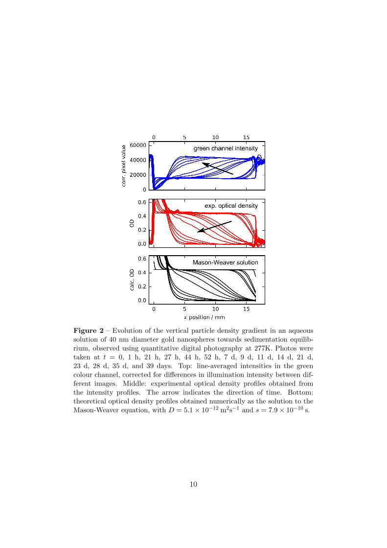
Figure 2 – Evolution of the vertical particle density gradient in an aqueoussolution of 40 nm diameter gold nanospheres towards sedimentation equilib-rium, observed using quantitative digital photography at 277K. Photos weretaken at t = 0, 1 h, 21 h, 27 h, 44 h, 52 h, 7 d, 9 d, 11 d, 14 d, 21 d,23 d, 28 d, 35 d, and 39 days. Top: line-averaged intensities in the greencolour channel, corrected for differences in illumination intensity between dif-ferent images. Middle: experimental optical density profiles obtained fromthe intensity profiles. The arrow indicates the direction of time. Bottom:theoretical optical density profiles obtained numerically as the solution to theMason-Weaver equation, with D = 5.1× 10⁻¹² m2s−1 and s = 7.9× 10⁻¹⁰ s.
10

The back-illumination of the observation cells should be homogeneous,which is not entirely the case in our set-up. The small illumination inho-mogeneities are corrected for by the baseline correction we apply. Smalldeviations in camera positioning from photograph to photograph lead tochanges in optical path lengths across the spectroscopic cells. There arealso fluctuations in illumination intensity; these are small and averaged outwhen quantitatively analyzing the time-lapse series using the Mason-Weavermodel, but lead to additional noise. Stray light is present in the optical sys-tem, i.e. the dark zones of the image are not entirely devoid of light, whichlimits the maximum optical density that can be reliably measured. A specificoptical design with dedicated illumination and detection optics may improvethe analysis of the concentration gradient.
The long duration of the sedimentation in some samples calls for effi-cient sealing of the containers, since solvent evaporation reduces the liquidcolumn height, introducing further uncertaintity in the analysis. Also, thethe meniscus at the top of the liquid column and the optical artefacts (darkzone) related to it limit the precision of the measurement of the gradient.
At present, the numerical analysis assumes an ideally monodisperse dis-tribution of nanoparticles, all being of the same shape and volume. Thediffusion and sedimentation coefficients obtained are effective, average coef-ficients. We have not attempted to analyse the data in terms of continuoussize distributions, in which case an additional weighting should be applied forthe strong dependence of the optical extinction coefficient on the diameterof gold nanoparticles.[39]
There is no fundamental impediment to analyzing the time-lapse opticalextinction profile data sets using models based on continuous polydispersesize distributions, or even multimodal distributions, similarly to what is cur-rently already done in analytical ultracentrifugation.[15, 20, 36] The numeri-cal solver presented here may be used to generate time-resolved concentrationprofiles for individual nanoparticle diameters in a trial distribution. Afterweighting with the effective extinction coefficients these can then be com-bined into the expected overall optical extinction profiles, which can then beoptimised to fit the experimental data. In this respect, multimodal size dis-tributions may be challenging if the different populations display unsufficientcontrast in diffusion and sedimentation coefficients.
11

Figure 3 – Diffusion D and sedimentation s coefficients obtained by analysingthe evolving experimental density gradient of settling gold nanosphere solu-tions (square markers). The solid curves are the expected values for per-fect golden spheres from the Stokes-Einstein-Sutherland equation (top), andStokes’ law (bottom). The dotted curves are for gold spheres with a hypo-thetical 1 nm thick organic layer.
12

4 Application to nanoparticle assemblies
After the initial demonstration of the quantitative analysis of time-lapse pho-tography of settling spherical gold nanoparticles in water, we investigated asample of purified DNA-linked dimers of 13 nm diameter gold nanospheres(Figure 4). This experiment illustrates that studying sedimentation canaid in the chemistry and characterization of biomolecularly-scaffolded multi-nanoparticle assemblies.
Figure 4 – Top left: transmission electron micrograph of purified DNA-linkeddimer sample. Top right: composed image of the time-lapse photography ofsedimenting DNA-linked gold nanosphere dimers (at 277 K). The rightmostcell is a sample of monomeric 13 nm gold nanospheres. Bottom: optical densitytraces as a function of vertical position in the cell, taken at various points intime (red solid lines); the black dotted curves are the solution to the Mason-Weaver equation with D = 5.8× 10⁻¹² m2 s−1 and s = 9.0× 10⁻¹¹ s
.
By adjusting the curves to the experimental data, we obtain D = 5.8 ×10⁻¹² m2 s−1 and s = 9.0× 10⁻¹¹ s, for the diffusion and sedimentation coef-ficients, respectively. The sedimentation coefficient of DNA-linked dimers isslightly smaller than that of a bare 13 nm monomer sphere, i.e. it sedimentseven more slowly. The extra mass from the second gold sphere is counter-balanced by more friction with the solvent due to the larger outer surfacearea of the dimer. The larger volume comes to a large extent from the DNA
13

which has a much lower density than gold.Additionally, the diffusion coefficient is lower than that of a 13 nm monomer
as a result of the larger hydrodynamic volume of the object. For the char-acteristic height (Eqn. 3) we find z0 = 6.6 mm. This value is close to whatwe would expect for an object which simply has the double buoyant massof a 13 nm monomer. Since gold has a much higher density than water,whereas the DNA linker has a density comparatively very close to that ofwater. Any extra volume taken up by the DNA linkage does not significantlycontribute to the buoyant mass of the object, since the displaced water vol-ume is replaced with a substance having a density close to that of water. Thebuoyant mass of the dimer is therefore determined by the two gold cores. Onthe other hand, the bulky DNA structure should indeed have an effect onthe sedimentation and diffusion constants, i.e. sedimentation will be greatlyslowed down compared to an equivalent sphere of the same buoyant mass.
The lower sedimentation coefficients leads to slower establishment of thegradient. However, in combination with the lower diffusion coefficient, itfinally leads to a more pronounced, shorter density gradient. A further anal-ysis of the hydrodynamic behaviour and the resulting combination of D ands of this type of assemblies is not within the scope of this work, but hasreceived recent attention in the literature.[19]
It is also interesting to note that the estimated time to obtain the finalequilibrium gradient (at 277K, with 2 cm liquid height) is on the order of 200days for both the monomers and the DNA-linked dimers. For analysing thetransient concentration profile it is not necessary to wait that long, whichdemonstrates the interest of having the numerical solution to the Mason-Weaver at hand. Nonetheless, 30 days is still a long time, and these samplesare better analysed with centrifuge-based techniques.[14, 16, 19, 24, 25, 40].In this context, it is interesting to note that — as we will see in the following— the required centrifugal acceleration for many inorganic-core nanoparticlesis well within range of standard laboratory centrifuges, instead of higher-speed specialised instruments.
5 Centrifugation of nanoparticle solutions
The results from the Mason-Weaver model may be used to generate intial ap-proximate estimates for preparative and analytical centrifugation. For manynano-assemblies using high-density inorganic core materials, the centrifugalacceleration necessary for rapid sedimentation is well within the capabilitiesof standard table-top laboratory centrifuges. A centrifugal acceleration thatis much higher than strictly necessary may have deleterious consequences
14

for colloidal stability as the density of nanoparticles in the pellet may be-come very high, accelerating aggregation. This is one reason why even arough estimate is of interest. Furthermore, we anticipate that preparativepurification protocols may be developed for nanoparticle assemblies by usingapproximate numerical simulations, using the computer code supplied withthe present work.
As an example we consider the minimal centrifugal acceleration gcfg neededto obtain sedimentation equilibrium for gold colloid solutions in a centrifugewithin a given time tcfg, i.e. we wish to establish the centrifugal conditionsfor a typical nanoparticle ‘centrifugation/re-dispersal’ washing procedure. InSection 2 of this paper, we found that the time to reach equilibrium is 1.4tsed,and using Eqn. (12) we can roughly estimate the centrifugal acceleration gcfg
necessary for the chosen centrifugation time tcfg and a liquid height in thecentrifuge tube ztube.
gcfg =1.4× ztube
s× tcfg
(13)
This can be expressed as ‘relative centrifugal force’ (‘times g’, RCF =gcfg/g, where g = 9.81 m s−1).
RCF =1.4× ztube
g × s× tcfg
(14)
As discussed above and detailed in the Supporting Information, the factor1.4 represents a conservative rough estimate of the time to reach equilibrium.This factor may become smaller as a function of the particle’s sedimentationand diffusion coefficients and the container height, using the formula by VanHolde and Baldwin,[38] or using results from numerical simulation. However,for the sake of simplicity, we will use 1.4 for the following calculations, asthis is a robust albeit conservative choice.
Table 2 contains the calculated RCF values needed for complete cen-trifugation of gold colloids in typical Eppendorf-type vials (liquid heightztube = 3 cm), within tcfg = 30 min. These values were then used in anexperiment in which a selection of colloidal gold solutions were spun for30 min. at the calculated RCF. The samples were subjected to a typicalcentrifugation/re-dispersal cycle, in which 95 vol% of the supernatant wasremoved, followed by redispersal of the (relatively fluid, but highly concen-trated) pellet in fresh water. In most cases the recommended centrifugalacceleration gave remarkably good results (Supporting Information, FigureS7).
Measurement of the UV-visible extinction spectra of the resuspended col-loids confirms the visual impression that the calculated RCF values are indeed
15

Table 2 – Calculated RCF values for complete centrifugation, within 30 min.,of spherical gold nanoparticles in water, using a liquid height of 3 cm. Ex-perimentally determined nanoparticle recovery in a typical centrifugation/re-dispersal washing cycle (n.t. = not tested).
diam. calcd. exp.(nm) RCF % recovery13 11671 n.t.20 4931 94 (a)40 1233 n.t.50 789 9860 548 n.t.80 308 97150 88 97(a) recovery increases to 97% by spinning at 1.2 timesthe calculated RCF
sufficient, and higher speeds for centrifugation are not necessary. In the caseof 20 nm diameter gold spheres, centrifugation at slightly higher acceleration(∼ 20%) was required to concentrate all particles near the bottom of thetube (Supporting Information, Figure S7).
Centrifugation at a given RCF corresponds to a sedimentation gradientlength scale zcfg
0 and corresponding concentration factor Bcfg. The gradientlength should be small enough, such that the nanoparticles are concentratedwell in the pellet. The concentration factor gives an estimate of the concen-tration increase at the bottom of the tube. For spherical particles, coefficients and D for Eqn. (15) are obtained from Eqn. (6).
zcfg0 =
D
s× g × RCFBcfg =
ztube
zcfg0 [1− exp(−ztube/z
cfg0 )]
(15)
For the conditions in Table 2 zcfg0 decreases from 2.1 µm (for 13 nm
diameter gold spheres) to well below 1 µm (larger particles), which indicatesthat the particles are well concentrated near the bottom of the tube.
Prolonged centrifugation may concentrate smaller particles of less densematerials. If we take for instance particles of 8 nm diameter with averagedensity 4.5×10³ kg m−3 in water (a rough estimate for typical[41] CdSe/ZnSquantum dot particles with a small-molecule capping), then it may be an-ticipated that these can be concentrated in a liquid pellet less than 300 µmhigh (zcfg
0 ∼ 31µm) by spinning them for 6 hours at 11000 × g (or 12 hoursat 5500 × g for a zcfg
0 ∼ 63µm), starting from a 3 cm liquid height (typicalEppendorf-type vial). Such centrifugation conditions are well in the range of
16

standard laboratory centrifuges.We may use similar reasoning to find the conditions for minimal centrifu-
gal stress, which will correspond to finding the minimum RCF necessary fora certain pellet compactness (small zcfg
0 ), and applying prolonged centrifuga-tion, the duration in that case given by tcfg.
Here, we were concerned with centrifugation without density gradient,starting from an initially homogeneous solution. For separation purposes,density gradient methods may be more adapted.[42] Moreover, we used theMason-Weaver model which assumes a constant gravitational field, insteadof the gradient found in centrifugation. Nevertheless, this simple model doesprovide a means of predicting the behaviour of nanoparticles in solution ina standard laboratory centrifuge, and is therefore relevant for the rationaldesign of nanoparticle purification protocols.
Another implication of this analysis is that the RCFs needed for thecentrifugal sedimentation of inorganic nanoparticles and their assemblies issignificantly lower than those in analytical ultracentrifuges (∼ 100000 × g).Analytical centrifugation using lower-speed (and simpler) equipment, suchas recent photocentrifuges with space- and time-resolved extinction profiling(STEP),[20–23] is therefore highly relevant for the characterization of inor-ganic nanoparticle solutions. Compared to the low-cost digital photography-based method presented here, such dedicated and optimised equipment pro-vide more rapid, precise and detailed analysis of nanoparticle samples.
6 Conclusion
This work rationalised observations on the settling of nanoparticles in liquidsolution in the framework of the Mason-Weaver model. This is illustrated bythe quantitative agreement between this model and experimental digital pho-tography for the time-evolution of the concentration gradient of suspendednanoparticles submitted to a gravitational field. A simple experimental pro-tocol for observing the sedimentation process is established, using time-lapsedigital photography of the samples in an undisturbed laboratory fridge inorder to avoid thermally induced convection.
By fitting a numerical solution of the Mason-Weaver equation to theexperimental concentration gradient, the diffusion and sedimentation coeffi-cients D and s are obtained, without need to wait for complete equilibrium tobe established. Early studies on sedimentation[3, 43] were mostly concernedwith precise measurement of the equilibrium gradient, which only yields thebuoyant mass mb of the particle as the sole parameter, not the separatecontributions of diffusion and sedimentation coefficients.
17

We demonstrated that measuring the evolving concentration gradient ofsettling solutions distinguishes between individual monomeric nanoparticlesand their dimeric assemblies, by giving a distinct combination of diffusionand sedimentation coefficients for each type of nano-object.
In our experiments on gold nanospheres in dilute solution, no signifi-cant deviations from the simple Mason-Waver model were observed. Col-loidal gold solutions are generally known to be well-behaved in this respect,and we expect many dilute solutions of other non-aggregating (inorganic)nanoparticles to behave in a similar way. Any significant deviations from thepredictions made by the Mason-Waver model would point to stronger inter-particle interactions, aggregation of individual objects, specific solvation[4–6]or surfactant[7, 8] effects, or changes in the properties of the liquid medium.It is important to be aware of such deviations as they may affect other as-pects of the behaviour of the nanoparticles in liquid media, such as theirinteraction with biological entities.
The simple mathematical model and the experimental protocol used herehave obvious limitations, and do not substitute advanced analytical centrifu-gation techniques[14, 16, 19–25, 40]. However, they do provide means for ini-tial and very simple screening of nanoparticle solutions, and rationalise visualobservations made at the bench, or upon prolonged storage in the laboratoryfridge. The use of a standard digital photo-camera limits the applicationsto systems that have detectable optical response in the visible. Many parti-cle systems do indeed have such a response, for instance plasmonic materialssuch as gold, silver, titanium nitride,[44] but also other metal particles, semi-conductor quantum dots,[17] and paramagnetic iron oxide.[29] Attainment ofequilibrium can take quite some time, and an analytical photocentrifuge[20–23] may be a time-saving investment, which also will yield more precise anal-ysis, in particular for broad size distributions and multimodal samples.
Based on the Mason-Weaver model, we obtained simple expressions thatgive useful recommendations for the centrifugation of nanoparticle solutions,so that delicate solutions can be processed with care, instead of spinning atmaximum RCF. The practical insights and simple quantitative expressionsprovided in the present work are of direct interest for wet-chemical synthesis,purification and application of functional nanoparticle assemblies, and willstimulate further interest in sedimentation analysis[4, 19, 23] for functionalnanoparticle solutions.
18

7 Experimental details
Temperature stabilisation. In a non-thermostated environment such asa lab shelf, even modest temperature changes may create temperature gra-dients in the sample that lead to convective motion sufficiently strong toprevent the sedimentation equilibrium from establishing itself. Such convec-tive motion plagued early sedimentation experiments, which were concernedwith precise measurement of the equilibrium distribution.[3, 43] Thermallydriven convection offers an explanation as to why, on a non-thermostatedshelf, many colloidal gold solutions seem not to evolve to a sedimentationequilibrium gradient. In the present work, mechanical and thermal per-turbations were avoided by carrying out the experiments in a undisturbedlaboratory fridge at 277 K.
Quantitative digital photography. In previous work we used quantita-tive colour imaging for measuring concentration profiles in microfluidic chan-nels, using an optical microscope and a dedicated CCD camera.[45] Here weuse a ’consumer-grade’ photo camera. Images were taken using a digitalcamera (Nikon Coolpix P7800, Nikon Corp., Japan) providing the outputof unprocessed (’RAW’) image data, where the individual pixel values areproportional to the detected light intensity for the particular colour chan-nel. This circumvents problems of linearization generally encountered withmost digital cameras.[31] Typically, four samples were photographed in asingle picture. A black area was also included to serve as the source forbackground subtraction.
The ’RAW’ image data were read by ImageJ software[46] using the dcrawplugin.[47] The three colour channels of the images were separated (ImageJ)and treated individually as monochrome intensity images. Intensity gradientprofiles Iraw(z) for all samples (and all colour channels) in each image ofthe time series were extracted by horizontal averaging over a rectangulararea (typically, the visible optical window of the cells). The pixel valuesof the black area were averaged for background substraction, Idark. Thez scaling was calibrated by precise measurements of specific cell features.Each image frame thus obtained its specific calibration of pixel size. Thedigital intensity profiles Iraw(z) were then further treated numerically usingthe Python programming language with scientific extensions.[48–50]
The individual profile traces with their specific z step sizes were re-sampled at a standard higher resolution in order to have profiles with identicalstep sizes, facilitating their processing and comparison with theory. Subse-quently, background-corrected image profiles I(z) were obtained by subtrac-tion of the near-zero dark background.
19

I(z) = Iraw(z)− Idark (16)
The top area of each extracted z profile, which does not contain liquid,was used for calculating I0 by averaging. This corrects slight frame-to-framevariations in illumination intensity. A linear baseline correction, ODbase(z) =k1z+k2, was applied globally to all time-frames for each sample. In all cases,the baseline correction was only modest and not necessary to obtain usefulresults.
The final corrected optical density is obtained using eqn. (17). We notethat we apply this Beer-Lambert-Bouguer formulation despite the conditionof monochromatic light not being rigorously fulfilled: the filters used in colourcameras define large spectral bands (width ∼ 100 nm). As has been discussedpreviously,[45] a linear response of the optical density as a function of concen-tration is still obtained, provided that the extinction spectra of the samplesare sufficiently large and their optical density is sufficiently low (under OD1).
OD(z) = log10
(I0
I(z)
)−ODbase(z) (17)
Comparison of experiment with theory is achieved by converting the con-centration profiles c(z) from the Mason-Weaver model into modeled opticaldensity profiles ODmodel(z) using an ”effective extinction coefficient” whichwe refer here to as k3 and can be adapted to rescale the model concentrationprofile to fit the experimental values.
ODmodel(z) = k3c(z) (18)
Centrifugation. A thermostated bench-top laboratory centrifuge (HettichMikro 220r with 1195-A rotor) was used. The relation between rotationalspeed (rounds per minute, RPM) and relative centrifugal force (RCF) is
RCF = 1.12× 10⁻³ ×R× (RPM)2 (19)
The rotor radius R for the 1195-A rotor used is 0.087 m. The maximumspeed for this rotor is 18000 RPM, corresponding to an RCF of 31500 × g.Samples were generally centrifuged with the centrifuge thermostat at 298K.
Colloidal gold solutions. For the study of the sedimentation of goldnanospheres (Section 3) we used standard aqueous solutions of colloidal goldfrom commercial sources (BBI Solutions, UK, and Sigma-Aldrich, France)and samples synthesised and characterised according to literature procedures.[51]
20

All colloids are stabilised with negatively charged carboxylate ligands, andthe particles have negative zeta potential. The samples were diluted withpure water where necessary. Typical optical densities at the extinction max-imum were in the range 0.3 . . . 1.
The carboxylate ligand layers around the particles are thin compared tothe particle diameter (d > 20 nm), and do not contribute significantly tothe buoyant mass. For smaller particles (< 10 nm) and larger ligands sucheffects may become significant, and will then show up as a deviation fromthe idealised predicted behaviour, and result in a change in effective buoyantmass, and effective diffusion and sedimentation coefficents. Furthermore, sol-vation effects on sedimentation may become significant, as the shell of solventmolecules around the object influences its hydrodynamic behaviour.[4–6]
DNA-linked dimers. The dimers were constructed from 13 nm gold nano-Gold nanoparticles of diameter 13 nm were synthesised according to the
published protocol.[52, 53] Briefly, a solution of sodium tetrachloroaurate (50mL, 1 mM) was heated up to 100 °C under stirring. Once boiling, a solution ofsodium citrate (5 mL, 2 wt.%) was added. After appearance of the typical redcolour, boiling and stirring were maintained for 15 additional minutes beforeletting cool down to room temperature. To stabilise the AuNPs, BSPP wasadded (15 mg) and the solution was left to stir overnight. TEM images wereobtained with a Hitachi H7000 transmission electron microscope, operatingat 75 kV bias. All samples preparation involved deposition and evaporationof a specimen droplet on a carbon film-coated 400 Mesh copper grid. TEManalysis is shown in the Supporting Information, Fig. S2.
Dimers of 13 nm AuNPs were synthesised using DNA hybridisation.[54]BSPP-coated AuNPs of 13 nm (5 pmol) were flocculated using NaCl andcentrifuged for 5 min at RCF 25 000× g (Eppendorf centrifuge 5417R, rotorFA-45-24-11, 8.8 cm radius). The supernatant was taken off and the particleswere re-dispersed in 100 µL buffer (20 mM phosphate, 5 mM NaCl). DNAsingle strands S1 respectively S2 (15 pmol) were added each to a separatenanoparticle solution to achieve a ratio DNA/particles of 3:1. A solution ofBSSP (10 µL, 1 mg/20 µL) was added and the reaction mixture was shakenfor 1 h, in order to deprotect the thiol group on the DNA and to allow itsattachment to the particles. The AuNPs were then centrifuged for 15 min at25 000 × g and redispersed in hybridization buffer (50 µL, 6mM phosphate,80mM NaCl). After mixing the two types of particles (S1 and S2 strands), acomplementary DNA strand S3 (2.5 pmol) was added to create the dimers.Hybridisation was realized by heating up the solution to 70°C and leaving itto cool down slowly and gradually to room temperature. The dimers werepurified by agarose gel electrophoresis (1.75% agarose gel in 0.5 x TBE, 1
21

h at 90V). After extraction from the gel the solution was centrifuged for 10min at 25 000× g and the dimers were redisolved in Milli-Q water.
Acknowledgements
This work was supported by Dstl (UK) in the framework of the France-UKPh.D. programme. MW acknowledges funding by the Agence Nationale dela Recherche (France), grant ANR-2010-JCJC-1005-1 (COMONSENS).
References
[1] M. D. Haw. J. Phys.: Condens. Matter 2002, 14, 33 7769.
[2] P. Ball. Chemistry World 2005, 2 38.
[3] J. Perrin. J. Phys. Theor. Appl. 1910, 9 5.
[4] J. W. Williams, K. E. Van Holde, R. L. Baldwin, H. Fujita. Chem. Rev.1958, 58, 4 715.
[5] T. M. Laue, W. F. Stafford III. Annu. Rev. Biophys. Biomol. Struct.1999, 28, 1 75.
[6] J.-J. Huang, Y. J. Yuan. Phys. Chem. Chem. Phys. 2016, 18, 17 12312.
[7] J. T. Li, K. D. Caldwell. Langmuir 1991, 7, 10 2034.
[8] M. Andersson, K. Fromell, E. Gullberg, P. Artursson, K. D. Caldwell.Anal. Chem. 2005, 77, 17 5488.
[9] V. Sharma, K. Park, M. Srinivasarao. Proc. Nat. Acad. Sci. 2009, 106,13 4981.
[10] K. Park, H. Koerner, R. A. Vaia. Nano Lett. 2010, 10, 4 1433.
[11] L. Scarabelli, M. Coronado-Puchau, J. J. Giner-Casares, J. Langer,L. M. Liz-Marzan. ACS Nano 2014, 8, 6 5833.
[12] F. Liebig, R. M. Sarhan, C. Prietzel, A. Reinecke, J. Koetz. RSC Adv.2016, 6, 40 33561.
[13] E. C. Cho, Q. Zhang, Y. Xia. Nat. Nanotechnol. 2011, 6, 6 385.
22
[14] J. M. Zook, V. Rastogi, R. I. MacCuspie, A. M. Keene, J. Fagan. ACSNano 2011, 5, 10 8070.
[15] R. P. Carney, J. Y. Kim, H. Qian, R. Jin, H. Mehenni, F. Stellacci,O. M. Bakr. Nat. Commun. 2011, 2, May 335.
[16] K. L. Planken, H. Colfen. Nanoscale 2010, 2, 10 1849.
[17] B. Demeler, T.-L. Nguyen, G. E. Gorbet, V. Schirf, E. H. Brookes,P. Mulvaney, A. O. El-Ballouli, J. Pan, O. M. Bakr, A. K. Demeler, B. I.Hernandez Uribe, N. Bhattarai, R. L. Whetten. Anal. Chem. 2014, 86,15 7688.
[18] J. Walter, K. Lohr, E. Karabudak, W. Reis, J. Mikhael, W. Peukert,W. Wohlleben, H. Colfen. ACS Nano 2014, 8, 9 8871.
[19] M. J. Urban, I. T. Holder, M. Schmid, V. Fernandez Espin, J. Garciade la Torre, J. S. Hartig, H. Colfen. ACS Nano 2016, 10 7418.
[20] T. Detloff, T. Sobisch, D. Lerche. Part. Part. Syst. Charact. 2006, 23184.
[21] T. Detloff, T. Sobisch, D. Lerche. Powder Technol. 2007, 174 50.
[22] E. Ibrahim, S. Hampel, J. Thomas, D. Haase, A. U. B. Wolter, V. O.Khavrus, C. Taschner, A. Leonhardt, B. Buchner. J. Nanoparticle Res.2012, 14 1118.
[23] J. Walter, T. Thajudeen, S. Suβ, D. Segets, W. Peukert. Nanoscale2015, 7 6574.
[24] Z. Krpetic, A. M. Davidson, M. Volk, R. Levy, M. Brust, D. L. Cooper.ACS Nano 2013, 7, 10 8881.
[25] A. Knauer, A. Thete, S. Li, H. Romanus, A. Csaki, W. Fritzsche, J. M.Kohler. Chem. Eng. J. 2011, 166, 3 1164.
[26] C. M. Alexander, J. C. Dabrowiak, J. Goodisman. J. Coll. Interf. Sci.2013, 396 53.
[27] C. M. Alexander, J. Goodisman. J. Coll. Interf. Sci. 2014, 418 103.
[28] A. I. Lopez-Lorente, M. Sieger, M. Valcarcel, B. Mizaikof. Anal. Chem.2014, 86 783.
23

[29] V. Prigiobbe, S. Ko, C. Huh, S. L. Bryant. J. Coll. Interf. Sci. 2015,447 58.
[30] M. Stevens, C. A. Paraga, I. C. Cuthill, J. C. Partridge, T. S. Troscianko.Biol. J. Linn. Soc. 2007, 90, 2 211.
[31] J. E. Garcia, A. G. Dyer, A. D. Greentree, G. Spring, P. A. Wilksch.PLoS ONE 2013, 8, 11 e79534.
[32] T. Schwaebel, O. Trapp, U. H. F. Bunz. Chem. Sci. 2013, 4, 1 273.
[33] M. Mason, W. Weaver. Phys. Rev. 1924, 23 412.
[34] O. Lamm. Ark. Mat. Astron. Fys. 1929, 21B 1.
[35] P. H. Brown, P. Schuck. Comp. Phys. Commun. 2008, 178, 2 105.
[36] P. Schuck. Biophys. J. 2000, 78, 3 1606.
[37] W. Weaver. Phys. Rev. 1926, 27, 4 499.
[38] K. E. Van Holde, R. L. Baldwin. J. Phys. Chem. 1958, 62, 6 734.
[39] J. R. G. Navarro, M. H. V. Werts. Analyst 2013, 138 583.
[40] J. B. Falabella, T. J. Cho, D. C. Ripple, V. A. Hackley, M. J. Tarlov.Langmuir 2010, 26, 15 12740.
[41] A. R. Clapp, E. R. Goldman, H. Mattoussi. Nat. Protoc. 2006, 1, 31258.
[42] B. Kowalczyk, I. Lagzi, B. A. Grzybowski. Curr. Opinion Coll. Interf.Sci. 2011, 16, 2 135.
[43] N. Johnston, L. G. Howell. Phys. Rev. 1930, 35 274.
[44] U. Guler, S. Suslov, A. V. Kildishev, A. Boltasseva, V. M. Shalaev.Nanophotonics 2015, 4, 3 269.
[45] M. H. V. Werts, V. Raimbault, R. Texier-Picard, R. Poizat, O. Francais,L. Griscom, J. R. G. Navarro. Lab. Chip 2012, 12 808.
[46] C. A. Schneider, W. S. Rasband, K. W. Eliceiri. Nat. Methods 2012, 9671.
[47] D. Coffin. dcraw. URL http://www.cybercom.net/~coffin/dcraw/.
24

[48] K. J. Millman, M. Aivazis. Comp. Sci. Eng. 2011, 13, 2 9.
[49] S. Van Der Walt, S. C. Colbert, G. Varoquaux. Comp. Sci. Eng. 2011,13, 2 22.
[50] J. D. Hunter. Comp. Sci. Eng. 2007, 9 90.
[51] N. G. Bastus, J. Comenge, V. Puntes. Langmuir 2011, 27, 17 11098.
[52] J. Turkevich, P. C. Stevenson, J. Hillier. Discuss. Faraday Soc. 1951,11, c 55.
[53] J. Turkevich, P. C. Stevenson, J. Hillier. J. Phys. Chem. 1953, 57, 7670.
[54] A. Heuer-Jungemann, R. Kirkwood, A. H. El-Sagheer, T. Brown, A. G.Kanaras. Nanoscale 2013, 5, 16 7209.
25

Supporting Information
for Part. Part. Syst. Charact. 2017, 1700095DOI: 10.1002/ppsc201700095
The sedimentation of colloidal nanoparticles in solution and itsstudy using quantitative digital photography
Johanna Midelet, Afaf H. El-Sagheer, Tom Brown,Antonios G. Kanaras and Martinus H. V. Werts*
S.1 Synthesis of DNA-linked gold nanosphere dimers
Figure S1 – Schematic of the assembly of DNA-linked dimers and subsequent’click’ chemistry.
.
S1

Table S1 – Sequences of single DNA strands S1, S2 and S3.
Figure S2 – Citrate-stabilised gold nanoparticles used for the construction ofDNA-linked dimers. a) TEM image of 13±2 nm spherical gold nanoparticles.Scale bar is 100 nm. b) Corresponding size distribution histogram, N = 500particles
.
S2

S.2 Finite-difference solver for the Mason-Weaver equa-tion
S.2.1 Dimensionless Mason-Weaver equation
A numerical solver has been designed for the dimensionless version of theMason-Weaver equation. Conversion between the Mason-Weaver equationand its dimensionless form can be achieved using:
ζ = z/z0 z0 =D
sg(S1)
and
τ = t/t0 t0 =D
s2g2(S2)
The aim is now to obtain the time-evolving spatial concentration distribu-tion c(ζ, τ) obeying the dimensionless Mason-Weaver equation (S3), startingfrom an arbitrary initial concentration profile c(ζ, 0).
∂c
∂τ=∂2c
∂ζ2+∂c
∂ζ(S3)
∂c
∂ζ+ c = 0 @ ζ = 0, ζ = ζmax (S4)
A finite-difference scheme for numerically solving this equation has beenproposed previously,[26] but unfortunately, in our hands, this did not yield aworking computer code. In particular, the proposed time coordinate trans-formation leads to unsurmountable numerical problems in our implementa-tion. Here, we propose a different finite-difference approximation that yieldsa stable, robust numerical solver, that moreover does not suffer from massconservation problems reported[26] for the previously proposed scheme.
S.2.2 Crank-Nicolson scheme
Time and space are discretised into N +1 and J+1 grid points, respectively.Space is on an evenly spaced grid between 0 and ζmax.
ζj = j∆ζ (j = 0, 1 . . . J) (S5)
∆ζ =ζmax
J(S6)
S3

Time may be on an evenly or unevenly spaced grid. We use an exponen-tially expanding grid, going from 0 to τmax.
τn = exp(kn)− 1 (n = 0, 1 . . . N) (S7)
k =ln(τmax + 1)
N
We make the following Crank-Nicolson style finite-difference approxima-tions for the PDE, where cnj is the value of c(ζj, τn).
∂c
∂τ→ γ(cn+1
j − cnj ) (S8)
∂2c
∂ζ2→ α(cnj+1 − 2cnj + cnj−1 + cn+1
j+1 − 2cn+1j + cn+1
j−1 ) (S9)
∂c
∂ζ→ β(cnj+1 − cnj−1 + cn+1
j+1 − cn+1j−1 ) (S10)
where (noting the factors 2 and 4 in α and β)
γ =1
τn+1 − τnα =
1
2(∆ζ)2β =
1
4∆ζ(S11)
With these finite-difference approximations, and after rearrangement ofthe terms, the discrete Mason-Weaver equation can be written as follows(j = 1, 2 . . . J − 1).
(−α + β)cn+1j−1 + (γ + 2α)cn+1
j + (−α− β)cn+1j+1
= (α− β)cnj−1 + (γ − 2α)cnj + (α + β)cnj+1 (S12)
The boundary conditions are set as follows. At ζ = 0 we choose
c→ 14(cn0 + cn+1
0 + cn1 + cn+11 ) (S13)
∂c
∂ζ→ 2β(cn1 − cn0 + cn+1
1 − cn+10 ) (S14)
Approximation of c using (S13) (instead of simply taking the values atc0) leads to much better behaviour in terms of mass conservation (the sumover all cj), in particular at longer times.
After substitution and rearrangement this results in
S4

(−2β + 14)cn+1
0 + (2β + 14)cn+1
1 = (2β − 14)cn0 + (−2β − 1
4)cn1 (S15)
At ζ = ζmax the equivalent choice was made (using backward differenceinstead of forward difference, naturally).
The equations (discretised PDE and BCs) are assembled into a matrixequation involving tridiagonal matrices. Numerically solving this equationyields the cn+1
j from cnj , i.e. the concentration profile at time τn+1 usingthe concentration profile from time τn. Repeating the process, starting fromthe initial condition at τ0, yields the evolution of the concentration profile,obeying the Mason-Weaver equation.
S.2.3 Implementation
The finite-difference scheme was implemented using Python (with numpy forarray manipulation and sparse matrix routines from scipy). For brevity,we only give the solver code without any plotting, processing or storage ofresults. It consists of a single loop that generates the successive concentrationprofiles cnj at each τn, starting from the initial conditions at τ0.
# -*- coding: utf -8 -*-
import numpy as np
from scipy import sparse
from scipy.sparse import linalg
""" Solver for the adimensional Mason -Weaver equation.
The solution is calculated on an exponentially expanding time
grid (N+1 points), and an evenly spaced space grid (J+1 points ).
Input:
zeta_max (float ): adimensional height of the cell
tau_end (float): calculate solution from tau=0 to tau=tau_end
J (int): number of space points minus 1 on (linear) grid
N (int): number of time points minus 1 on (exponential) grid
Output:
The solution is stored in a two -dimensional array ’c’.
The space grid points are given by the vector ’zeta ’.
The time grid points are given by the vector ’tau ’.
code tested with Python 3.5.2, Anaconda 4.1.1 (64-bit)
"""
def _tridiamatrix(J,ldiagelem ,cdiagelem ,rdiagelem ,
S5

cstart ,rstart ,lend ,cend):
""" utility function that generates a sparse tridiagonal
matrix from given elements """
ldiag = np.empty(J+1)
cdiag = np.empty(J+1)
rdiag = np.empty(J+1)
ldiag.fill(ldiagelem)
cdiag.fill(cdiagelem)
rdiag.fill(rdiagelem)
cdiag [0]= cstart
rdiag [1]= rstart
ldiag [-2]= lend
cdiag [-1]= cend
diag=[ldiag ,cdiag ,rdiag]
N = J+1
return sparse.spdiags(diag ,[-1,0,1],N,N,format="csr")
# set calculation parameters
zeta_max = 10. # height of cell
tau_end = 10. # end tau
J = 400 # number of space points (-1)
N = 200 # number of time points (-1)
c_init = np.ones(J+1) # initial condition
# define time and space grids
k_tau = np.log(tau_end +1)/N
tau = -1.0 + np.exp(k_tau*np.arange(0,N+1))
dltzeta = zeta_max/J
zeta=np.linspace(0,zeta_max ,J+1,endpoint=True)
# create c array for storing result
c = np.zeros ((J+1,N+1))
c[:,0] = c_init
c_n = c_init
dltzeta=dltzeta
tau=tau
# loop generating c^{n+1} from c^{n} starting from c^0
for n in range(0,N):
alpha = 1/(2*( dltzeta **2))
beta = 1/(4* dltzeta)
gamma = 1/(tau[n+1]-tau[n])
# finite difference diagonals Left Hand Side
ldiagelem = -alpha + beta
cdiagelem = gamma + 2* alpha
rdiagelem = -alpha - beta
# boundary conditions LHS
cstart = -2*beta + 0.25
S6

rstart = 2*beta + 0.25
lend = -2*beta + 0.25
cend = 2*beta + 0.25
# create LHS tridiagonal matrix
LHSmat = _tridiamatrix(J,ldiagelem ,cdiagelem ,rdiagelem ,
cstart ,rstart ,lend ,cend)
# finite difference diagonals Right Hand Side
ldiagelem = alpha - beta
cdiagelem = gamma - 2*alpha
rdiagelem = alpha + beta
# boundary conditions RHS
cstart = 2*beta - 0.25
rstart = -2*beta - 0.25
lend = 2*beta - 0.25
cend = -2*beta - 0.25
# create RHS tridiagonal matrix
RHSmat = _tridiamatrix(J,ldiagelem ,cdiagelem ,rdiagelem ,
cstart ,rstart ,lend ,cend)
# construct RHS vector
RHSvec = RHSmat * c_n # c contains concentration profile
# SOLVE the matrix equation , giving c^{n+1} (c_next)
c_next = linalg.spsolve(LHSmat ,RHSvec)
# store c_{n+1} into solution matrix
c[:,n+1] = c_next
# we swap the vectors containing c_n and c_next via cswap
# we cannot simply re-assign c_n = c_next
cswap = c_n
c_n = c_next
c_next = cswap
# plot example
import matplotlib.pyplot as plt
plt.figure (1)
plt.clf()
for i in [0 ,50 ,100 ,150 ,200]:
plt.plot(zeta , c[:,i],label=’tau=’+str(tau[i]))
plt.ylim (0,3)
plt.xlabel(’$\\ zeta$ ’)
plt.ylabel(’$c$’)
plt.legend ()
plt.show()
S7

S.2.4 Validation of the numerical solution
The numerical solver was tested extensively for a wide range of ζmax andτ . Typical values for N and J were on the order of several hundred gridpoints. Numerical mass conservation and convergence of the gradient to theanalytical Boltzmann equilibrium solution were verified.
An example of a numerical solution is given in Figure S3, which alsoillustrates that the numerical solution faithfully converges to the analyticalequilibrium distribution, for τ = 1.4τsed.
Figure S3 – Left: Numerical solution (N = 200, J = 400) to the dimension-less Mason-Weaver equation with ζmax = 10 and τ going from 0 to 30. Right:Comparison of the analytical equilibrium profile and the numerical solutionat longer times, demonstrating (1) that the numerical solution converges tothe analytical equilibrium (Boltzmann) distribution and (2) that at 1.4τsed thesystem is virtually at equilibrium.
Mass conservation is observed in the numerical scheme, as illustrated inFigure S4. A slight increase of the total numerical mass is observed, but thenumerical solution does not diverge at longer simulation times, as a result ofour choice for the boundary conditions, cf. Equation (S13).
S8

Figure S4 – Evolution of the total mass in the numerically simulated system(N = 200, J = 400, ζmax = 10, τ = 0 . . . 30), obtained by summing all spacegrid points. A slight increase (< 2%) of the total numerical mass is observed,but the total mass does not diverge for long simulation times.
S9
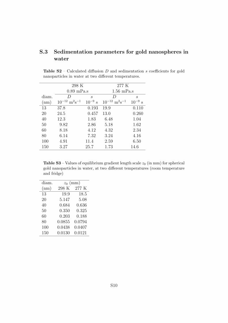
S.3 Sedimentation parameters for gold nanospheres inwater
Table S2 – Calculated diffusion D and sedimentation s coefficients for goldnanoparticles in water at two different temperatures.
298 K 277 K0.89 mPa.s 1.56 mPa.s
diam. D s D s(nm) 10−12 m2s−1 10−9 s 10−12 m2s−1 10−9 s13 37.8 0.193 19.9 0.11020 24.5 0.457 13.0 0.26040 12.3 1.83 6.48 1.0450 9.82 2.86 5.18 1.6260 8.18 4.12 4.32 2.3480 6.14 7.32 3.24 4.16100 4.91 11.4 2.59 6.50150 3.27 25.7 1.73 14.6
Table S3 – Values of equilibrium gradient length scale z0 (in mm) for sphericalgold nanoparticles in water, at two different temperatures (room temperatureand fridge)
diam. z0 (mm)(nm) 298 K 277 K13 19.9 18.520 5.147 5.0840 0.684 0.63650 0.350 0.32560 0.203 0.18880 0.0855 0.0794100 0.0438 0.0407150 0.0130 0.0121
S10

Table S4 – Calculated concentration factor B for spherical gold nanoparticlesin water at 277K (left columns) and 298K (right columns), for cell heights(zmax) of 1 mm and 1 cm
277K 298Kdiam. B(nm) 1 mm 1 cm 1 mm 1 cm13 1.03 1.29 1.03 1.2720 1.10 2.29 1.09 2.1840 1.99 15.7 1.90 14.650 3.22 30.7 3.03 28.660 5.34 53.1 4.97 49.480 12.6 126 11.7 117100 24.6 246 22.9 229150 83.0 830 77.1 771
Table S5 – Calculated sedimentation times (in hours) for gold nanoparticlesin water for a cell with zmax = 1 cm. A good rough estimate for the time toreach equilibrium is tequil ≈ 1.4tsed. These times are directly proportional tocell height.
diam. tsed(h)(nm) 298 K 277 K13 1465 258020 619 109040 155 27250 99.0 17460 68.8 12180 38.7 68.1100 24.8 43.6150 11.0 19.4
S11

S.4 The time needed to reach sedimentation equilib-rium
In the main text we state that a simple but robust approximation for thetime to reach sedimentation equilibrium is 1.4 times the time tsed needed bya particle to traverse the liquid column from top to bottom at its terminalsedimentation velocity. This approximation enables a simple estimate ofthe time needed for centrifugation of nanoparticles at a certain centrifugalacceleration.
A more sophisticated approach to this question is known in the ultra-centrifugation literature.[38] This approach by Van Holde and Baldwin[38]yields the time to arrive near equilibrium within a ’distance’ determined byparameter ε. The choice for this parameter made in [38] is based on thedifference in particle concentration between the top and the bottom of thecell, ∆c = c(0)− c(zmax).
ε = 1− ∆c(t)
∆ceq
(S16)
At the beginning, when the concentration is homogenous, ε = 1. Assedimentation equilibrium is reached ε will tend to zero. A close approach toequilibrium is typically obtained for ε < 0.02. The time to come within this’distance’ ε from equilibrium can then be approximated with the followingexpression.
tequil ≈z2
max
DF (α) (S17)
F (α) = − 1
π2U(α)ln
(π2U2(α)ε
4[1 + cosh(1/2α)]
)(S18)
U(α) = 1 +1
4π2α2(S19)
The time to reach equilibrium is expressed as a function of α, which, inthe context of the present work, is given by
α =kBT
mbgzmax
(S20)
An interesting point is that the parameter α can also be expressed as theratio from the length scale of the equilibrium gradient z0 to the height of theliquid column zmax.
S12

α =kBT
mbgzmax
=z0
zmax
(S21)
It is thus a measure of how the equilibrium gradient ’fits’ in the heightof the liquid column. For ’oversized’ containers (where all particles will fi-nally be concentrated near the bottom of the container), the attainment ofequilibrium for initial homogeneous distribution will be governed by the timeneeded for sedimentation, whereas containers much smaller than the equilib-rium gradient will not show much of the gradient, i.e. when α becomes verylarge, the gradient will be undetectable.
Equation (S17) may be expressed as the ratio of tequil and tsed. It can beshown that this ratio is a pure function of α. It thus depends only on theratio z0/zmax, not on D and s individually.
tequil
tsed
=F (α)
α(S22)
It is important to note that Equation (S17) is an approximation forα > 0.1,[38] and that it is not valid at smaller values. For small α ourapproximation tequil ≈ 1.4tsed is valid and safe. For α > 0.1, we find thatthe time predicted by Eqn (S17) is always shorter than the rough 1.4tsed
estimation (see Figure S5)
Figure S5 – Left: The ratio of the ‘time-to-equilibrium’ tequil and the ‘sedi-mentation time’ tsed as a function of parameter α. Curves (a) are calculatedusing Eqn. (S17), valid for α > 0.1. We chose ε = 0.018, such that themaximum of the curve is at 1.4. Curves (b) use the constant 1.4 ratio fromthis work. Right: Absolute sedimentation times in 2 cm high water column,calculated for spherical gold particles. T = 277.15 K was used. Small valuesof α (left) correspond to large particle diameters (right).
We note that our numerical solver enables full simulation of the sedimen-tation process. This can be used to study in more detail the evolution of theconcentration gradient and the attainment of equilibrium. A different metric
S13

for the distance to equilibrium may be used instead of the difference betweenthe two outermost points, such as the root-mean-square deviation over theentire curve, or a metric that is representative to the particular measurementused.
We performed numerical simulations of the attainment of sedimentationequilibrium for different values of α. The numerical solver allows us to studyalso the case of α < 0.1 not covered by Equation (S17). Figure S6, showshow the ‘distance to equilibrium’ ε (Eqn. S16) evolves over time (relativeto the sedimentation time tsed). For all values of α, equilibration is nearcompletion at t ≈ 1.4tsed, even for the ‘worst case’ α = 0.1. As predicted byEqn. (S17), equilibrium is attained relatively faster (t < 1.4tsed) for larger α(smaller particles).
Figure S6 – Approach to sedimentation equilibrium, obtained using the nu-merical Mason-Weaver solver, for different values of α. Equilibration is alwaysvirtually complete at t = 1.4tsed. For large α, time to equilibrium becomesshorter.
This brief analysis shows that tequil ≈ 1.4tsed is useful as a rough approx-imation. It never underestimates the time to equilibrium. However, it doesoverestimate the time to equilibrium for the smaller particles, in which caseEquation (S22) becomes relevant.
S14

S.5 Experimental test of the centrifugation parame-ters recommmended by the Mason-Weaver model
Figure S7 – Centrifugation of gold nanospheres in water, for 30 min. at thecentrifugal acceleration recommended by the Mason-Weaver model. Diame-ters: (a) 20 nm, (b) 50 nm, (c) 80 nm, (d) 150 nm. Photographs on the left:centrifuge vials before and after centrifugation. Relative centrifugal force: (a)4931 × g, (b) 789 × g, (c) 308 × g, (d) 88 × g. UV-visible extinction spectraon the right: sample before centrifugation (black) and after (blue) re-dispersalof the liquid pellet (5% of the initial volume); red: supernatant (95% of theinitial volume).
S15

Figure S8 – Centrifugation of 20 nm diameter gold nanospheres in water, for30 min., at 6000×g, i.e. 20% higher than the Mason-Weaver recommendation.
S16