the seismic analyzer: interpreting and illustrating 2d seismic...

The Seismic Analyzer: Interpreting and Illustrating 2D Seismic Data

Daniel Patel, Christopher Giertsen, John Thurmond, John Gjelberg, and M. Eduard Groller, Member, IEEE

Abstract—We present a toolbox for quickly interpreting and illustrating 2D slices of seismic volumetric reflection data. Searching foroil and gas involves creating a structural overview of seismic reflection data to identify hydrocarbon reservoirs. We improve the searchof seismic structures by precalculating the horizon structures of the seismic data prior to interpretation. We improve the annotationof seismic structures by applying novel illustrative rendering algorithms tailored to seismic data, such as deformed texturing and lineand texture transfer functions. The illustrative rendering results in multi-attribute and scale invariant visualizations where features arerepresented clearly in both highly zoomed in and zoomed out views. Thumbnail views in combination with interactive appearancecontrol allows for a quick overview of the data before detailed interpretation takes place. These techniques help reduce the work ofseismic illustrators and interpreters.

Index Terms—Seismic interpretation, Illustrative rendering, Seismic attributes, Top-down interpretation

1 INTRODUCTION

Oil and gas are valuable resources accounting for around 64% of thetotal world energy consumption [10]. Oil and gas search and recoveryis an economically valuable but complex task. Imaging the subsurfacefor exploration purposes is highly expensive. The imaging surveysconsist of sending sound waves into the earth and recording and pro-cessing the echoes. Throughout the article we refer to this processeddata as the seismic reflection data.

Due to the measuring expenses, an iterative approach for collectingdata is taken. The first stage of a search typically involves collectingmultiple 2D seismic slices which are analyzed by a team of geolo-gists and geophysicists. If an area showing signs of hydrocarbons isdiscovered, 3D seismic reflection data is collected and analyzed. Iffurther indications of hydrocarbon accumulation are found in the newdata, drilling a well might be considered. Irrespective if the drillinghits a reservoir or not, it will give deeper insight into the data due tothe process of bore hole logging. A bore hole log consists of phys-ical measurements along the well path such as mineral conductivity,radioactivity and magnetism.

The current work flow in searching for oil and gas is to start a de-tailed interpretation of seismic structures. When enough structureshave been interpreted to get an overview of the data, the results arediscussed by an interdisciplinary team. This bottom-up approach istime consuming. The interpretation is challenging due to the low res-olution and noisy nature of the seismic data. In cases of doubt, theinterpreter often creates several alternatives of the same seismic struc-ture. In addition, it is not uncommon that the team disagrees on theinterpretation and decides that parts of the data must be reinterpreted.As soon as a consensus is achieved, the interpretation is documentedfor further dissemination outside the team. As part of the documenta-tion, a seismic illustrator draws illustrations of the interpretation. Tra-ditional illustrating is a time-intensive task and is therefore done latein the work flow.

• Daniel Patel is with Christian Michelsen Research, Bergen, Norway,E-mail: [email protected].

• Christopher Giertsen is with Christian Michelsen Research, Bergen,Norway, E-mail: [email protected].

• John Thurmond is with StatoilHydro, Bergen, Norway, E-mail:[email protected].

• John Gjelberg is with StatoilHydro, Bergen, Norway, E-mail:[email protected].

• Eduard Groller is with Vienna University of Technology, Austria, E-mail:[email protected].

Manuscript received 31 March 2008; accepted 1 August 2008; posted online19 October 2008; mailed on 13 October 2008.For information on obtaining reprints of this article, please sende-mailto:[email protected].

In this work we present a top-down interpretation approach as astep prior to the currently used bottom-up interpretation. This alle-viates some of the issues in the bottom-up approach. The top-downinterpretation is performed with a sketching tool that supports coarseinterpretation and quick creation of communication-friendly seismicillustrations. The inaccuracy in the seismic data and the need for pre-ciseness during bottom-up interpretation can easily lead the interpreterto wrong conclusions based on insufficient information. When rein-terpretation is required due to wrong conclusions, the long time lapsesbetween interpretation and meetings is a big problem. With our top-down procedure, we facilitate short interpretation-to-meeting cycles.This enables earlier and more frequent discussions of interpretationhypotheses. Hypotheses can be clearly annotated, presented and pos-sibly discarded earlier. A common understanding of the data can beachieved before the detailed interpretation starts. This can reduce theneed for reinterpretations during the bottom-up approach. One cansave time identifying which structures to focus on during the bottom-up interpretation. Also, no tools for quickly creating seismic illustra-tions exist. Currently general drawing software is used to illustrateseismic slices.

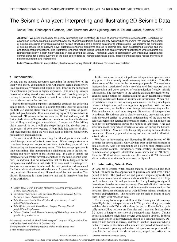
We focus on interpreting and illustrating 2D slices instead of 3Dvolumes for several reasons. Only 2D data exist in the earliest stage ofdata collection. Also it is common to do a slice by slice interpretationof the seismic volume. Furthermore, when creating illustrations forcommunication purposes, illustrators make heavy use of 2D slices.Even for 3D illustrations, cutouts are often used with 2D illustratedslices on the cutout side surfaces as seen in Figure 1.

1.1 Interpreting Seismic DataOil and gas is created when organic material is deposited and thenburied, followed by the application of pressure and heat over a longperiod of time. The produced oil and gas will migrate upwards andaccumulate in reservoir structures such as anticlines (seen in left Fig-ure 1) or fault traps. Oil and gas is searched for by looking for signs ofthese depositional or reservoir structures. Due to the limited resolutionof seismic data, one must work with interpretable events such as thehorizons. Horizons delineate rocks with different mineral densities orporosity characteristics. The horizons can be seen as bright or darklines in gray-level reflection data.

The existing bottom-up work flow at the Norwegian oil companyStatoilHydro is to interpret about each 25th yz slice along the x-axisand then about each 25th xz slice along the y-axis. For each slice, typi-cally around 5 key horizons are identified and traced out. It takes about2-3 hours to interpret one slice of a standard-sized dataset. Certainpoints at a horizon might have several continuation options. In thesecases, each option is interpreted and stored as a separate horizon. De-ciding which horizon is correct, and which is not, is taken later when abetter overview exists. When all slices are interpreted, different meth-ods of automatic growing and surface interpolation are performed tocomplete the horizons in the slices that were jumped over. After an in-

1571

1077-2626/08/$25.00 © 2008 IEEE Published by the IEEE Computer Society

IEEE TRANSACTIONS ON VISUALIZATION AND COMPUTER GRAPHICS, VOL. 14, NO. 6, NOVEMBER/DECEMBER 2008

Manuscript received 31 March 2008; accepted 1 August 2008; posted online 19 October 2008; mailed on 13 October 2008. For information on obtaining reprints of this article, please send e-mail to: [email protected].

Authorized licensed use limited to: IEEE Xplore. Downloaded on November 21, 2008 at 17:45 from IEEE Xplore. Restrictions apply.

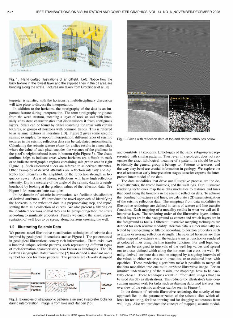
Fig. 1. Hand crafted illustrations of an oilfield. Left: Notice how thebrick texture in the lowest layer and the stippled lines in the oil area arebending along the strata. Pictures are taken from Grotzinger et al. [8]

terpreter is satisfied with the horizons, a multidisciplinary discussionwill take place to discuss the interpretation.

In addition to the horizons, the stratigraphy of the data is an im-portant feature during interpretation. The term stratigraphy originatesfrom the word stratum, meaning a layer of rock or soil with inter-nally consistent characteristics that distinguishes it from contiguouslayers. Strata can be found by either searching for areas with certaintextures, or groups of horizons with common trends. This is referredto as seismic textures in literature [10]. Figure 2 gives some specificseismic examples. To support interpretation, different types of seismictextures in the seismic reflection data can be calculated automatically.Calculating the seismic texture chaos for a slice results in a new slicewhere the value of each pixel encodes the variance of the gradients inthe pixel’s neighbourhood (seen in bottom right Figure 3). The chaosattribute helps to indicate areas where horizons are difficult to trackor to indicate stratigraphic regions containing salt (white area in rightFigure 1). Such calculated slices are referred to as derived attributes.Other examples of derived attributes are reflection intensity and dip.Reflection intensity is the amplitude of the reflection strength in fre-quency space. Areas of strong reflections will have high reflectionintensity. Dip is a measure of the angle of the seismic data in a neigh-bourhood by looking at the gradient values of the reflection data. SeeFigure 3 for some attribute examples.

In the domain of seismic interpretation, we facilitate visualizationof derived attributes. We introduce the novel approach of identifyingthe horizons in the reflection data in a preprocessing step, and repre-senting them as a collection of curves. We also present a filtering onthe identified horizons so that they can be grouped together into strataaccording to similarity properties. Finally we enable the visual repre-sentation of well logs to be spread along horizons crossing the well.

1.2 Illustrating Seismic DataWe present novel illustrative visualization techniques of seismic datainspired by geological illustrations such as Figure 1. The patterns usedin geological illustrations convey rich information. There exist overa hundred unique seismic patterns, each representing different typesof rock-formation characteristics, also known as lithologies. The USFederal Geographic Data Committee [2] has defined a standard and asymbol lexicon for these patterns. The patterns are cleverly designed

Fig. 2. Examples of stratigraphic patterns a seismic interpreter looks forduring interpretation. Image is from Iske and Randen [10].

Fig. 3. Slices with reflection data at top and derived attributes below.

and constitute a taxonomy. Lithologies of the same subgroup are rep-resented with similar patterns. Thus, even if a geologist does not rec-ognize the exact lithological meaning of a pattern, he should be ableto identify the general group it belongs to. Patterns or textures, andthe way they bend are crucial information in geology. We explore theuse of textures at early interpretation stages to easier express the inter-preters inner model of the data.

The data modalities that drive our illustrative process are the de-rived attributes, the traced horizons, and the well logs. Our illustrativerendering techniques map these data modalities to textures and linesthat bend along the horizons in the seismic reflection data. To achievethe ’bending’ of textures and lines, we calculate a 2D parameterizationof the seismic reflection data. The mappings from data modalities toillustrative renderings are defined in terms of texture and line transferfunctions. Each mapping of a modality results in what we call an il-lustrative layer. The rendering order of the illustrative layers defineswhich layers are in the background as context and which layers are inthe foreground as focus. Different illustrative mapping techniques aredefined for each seismic modality. Horizon data is either manually se-lected by user-picking or filtered according to horizon properties suchas angles or average reflection strength. The selected horizons are theneither mapped to textures with the texture transfer function or renderedas coloured lines using the line transfer function. For well logs, tex-tures can be assigned to intervals of the well log values and spreadout to a user-defined width along the horizons that cross the well. Fi-nally, derived attribute data can be mapped by assigning intervals ofthe values to either textures with opacities, or to coloured lines withopacities. These rendering algorithms make it possible to merge allthe data modalities into one multi-attribute illustrative image. For anintuitive understanding of the results, the mappings have to be care-fully chosen. These techniques result in informative images that canbe used directly as illustrations. This reduces the illustrator’s time con-suming manual work for tasks such as drawing deformed textures. Anoverview of the seismic analyzer can be seen in Figure 4.

In the domain of seismic illustrative rendering, the novelty of ourapproach lies in the parameterization of the seismic slice which al-lows for texturing, for line drawing and for dragging out textures fromwell logs. Also we introduce the concept of mapping seismic modal-

1572 IEEE TRANSACTIONS ON VISUALIZATION AND COMPUTER GRAPHICS, VOL. 14, NO. 6, NOVEMBER/DECEMBER 2008


Fig. 4. The seismic analyzer. The brown rounded rectangles representour algorithms and refer to the sections describing them. The ’seismicsurveys’ rectangle represents the process of obtaining the seismic data.The ’derive attributes’ rectangle represents the process of deriving at-tributes using external software.

ities to illustrative layers which achieves multi-attribute visualization,illustrative visualization, and scale invariance.

2 RELATED WORK

Several papers discuss processing and visualization algorithms for 3Dseismic data. The visualization algorithms presented in papers and incommercial solutions are mostly direct volume rendering of the seis-mic data and surface rendering of interpreted objects such as horizons.In slice visualizations, horizons are represented as lines. For accu-rate structural interpretation, some papers deal with horizon extractionas in Castanie et al. [5] or fault extraction as in Jeong et al. [11] andGibson et al. [7]. Pepper and Bejarano [15] give an overview of auto-matic interpretation methods. Plate et al. [16] and Castanie et al. [5]deal with handling large seismic volumes. Ropinski et al. [18] covervolume rendering of seismic data in VR. They present spherical andcubic cutouts which have a different transfer function than the sur-rounding volume. Commercial software used in oil companies includeHydroVR [13] and Petrel [1]. None of these works deal with illustra-tive techniques or top-down interpretation as presented here. Papersthat cover horizon extraction do it semi-automatically. The user hasto select a seedpoint from where the horizon will be grown accordingto some user defined connectivity criteria. Our work differs in that weautomatically pre-grow all horizons.

In our previous work [14] illustrative techniques for seismic datawas also presented. That work dealt with the presentation and valida-tion of interpreted seismic data. In this work we introduce a toolbox

for interpreting and illustrating non-interpreted seismic data. This pro-vides stronger illustrating capabilities than in our previous work. Theparameterization in the previous work [14] required manually inter-preted complete horizons. Now we introduce a parameterization thatworks directly on uninterpreted data by accepting automatically cre-ated horizon patches. We extend the texture transfer function from theprevious work by introducing a flexible GUI and layered illustrativetransfer functions for lines, wells and the automatically extracted hori-zons. Furthermore we propose how these techniques can be used inconcert to improve the current work flow in oil companies by intro-ducing the concept of top-down interpretation.

The 2D parameterization we present in this paper differs from pa-rameterization methods used for texturing in other domains. 2D tex-tures are applied to 2D images in both vector field visualization, suchas Taponecco et al. [19], and in brush stroke synthesis as in Hays andEssa [9]. Our method differs in that we calculate the texture bend-ing so it follows structures specific to seismic reflection data and notgeneral gradient trends or edges. How we create the 2D parameteri-zation is also different. Taponecco et al. [19] create 1D lines that areparameterized in length and then expanded in thickness to create a 2Dparameterization. This procedure is performed locally over a collec-tion of evenly distributed lines that cover the 2D image. This howeverresults in overlapping textures. Our method considers the 2D spaceglobally to create a complete and non-overlapping parameterization.

Much work has been done in multi-attribute visualization, Burgeret al. [4] present a state of the art overview. Crawfis and Allison [6]present a general framework where textures, bump maps and contourlines are used for multi-attribute visualization. Kirby et al. [12] presentmulti-attribute visualization of 2D flows using concepts from painting.They visualize flow attributes using procedural glyphs on a colour-coded background. Taylor [20] takes a general approach by combin-ing colour, transparency, contour lines, textures and spot noise. Hesucceeds in visualizing four attributes simultaneously. However, littlework has been done in multi-attribute visualization of seismic data.

3 EXTRACTING HORIZONS AND PARAMETERIZING THE RE-FLECTION DATA

In this section we describe how the horizon structures are found andhow the 2D parameterization is calculated. The horizon lines are useddirectly in the visualization of the data and as input to the 2D param-eterization. The horizons and the parameterization is calculated in apreprocessing step prior to the visualization.

3.1 Tracing the Horizons

We adapt the method described in Iske and Randen [10] to trace outhorizons. By considering the seismic reflection data as a height field,the horizons are running along valleys and ridges of the height field.We automatically trace out some of these valleys and ridges. Ourmethod differs from existing horizon tracing algorithms since it doesnot require a user defined seed point for each trace. We go through allsamples in the seismic slice and create traces for samples that are lo-cal maxima or minima in a vertical neighbourhood of 3 samples. Theresult is a collection of lines going through the horizons of the slice.

3.2 Parameterization of the Horizons

To achieve the effect of textures and lines following the orientationtrend of the underlying reflection data, we create a parameterizationfrom the traced horizons. The parameterization creates a relationshipbetween image space and parameter space as seen in Figure 5a and b.There are four steps in determining the parameterization. The first stepis to create suggestive line segments that indicate the horizons in thereflection data. We use the extracted horizon lines for this. The secondstep is to calculate the vertical v parameter values from the horizons.Thirdly, from the v parameter values, the horizontal u parameter valuesare calculated. Finally the u parameter values are normalized to mini-mize distortion in the parameterization. The parameterization processwill ensure that horizons are mapped to straight lines in parameterspace. Inversely, this guarantees that straight illustrative textures and

1573PATEL ET AL: THE SEISMIC ANALYZER: INTERPRETING AND ILLUSTRATING 2D SEISMIC DATA


Fig. 5. Relationship between image space (a), and parameter space (b).In (c) is shown the procedure of finding the u parameter for a point (redcircle) in image space by tracing from the point along a curve normal tothe v parameter until it hits a u parameterized v -isocurve.

straight lines in parameter space will be aligned with the horizons inimage space.

In the second step we calculate the v parameter by sweeping a ver-tical line from left to right over the horizons (Red line in Figure 6).The sweep line consists of a set of control points with unique v val-ues. Initially there is one control point at the bottom of the line withv=0 and one at the top with v=1. The v values between control pointsare linearly interpolated. As the sweep line moves to the right, it willintersect the horizon lines. At the position on the sweep line where itintersects the start of a horizon, a new control point is created (doublecircle) which is assigned the interpolated v value at that point on thesweep line. For the following intersections of the same horizon line,the associated control point will update its position according to theintersection but will keep its initially given v value. One can imag-ine the sweep line as a rubber ribbon getting hooked on and off thehorizons. After all points in the slice have been assigned v values, a2D smoothing is performed to smooth out the discontinuities that arisejust behind the horizon ends (see Figure).

Finding the u parameterization involves finding a mapping fromvertical lines in parameter space (vertical black line in Figure 5b) toimage space (Figure 5a). We want the parameterization to be anglepreserving so that for instance the 90 degree angles at the edges ofbricks in a brick texture are more or less preserved when mapped toimage space. For this to be fulfilled, we require that the vertical linesin parameter space are always normal to the v-isocurves. We find aninitial vertical line in parameter space by tracing two lines from themiddle of the image space (blue dot in Figure 5c), one in the normaldirection of the v parameterization, and one against the normal direc-tion. This line is then parameterized according to its curve length andis divided into intervals of length dv (yellow dots in Figure 5c). Fromeach of the interval ends (yellow dots) we span out v-isocurves. Eachv-isocurve is u-parameterized according to its curve length and is setto 0 at the intersection with the left image border. The image spacehas now been divided into strips. Finally, the u value for any point in

Fig. 6. Calculating the v parameterization by sweeping the red line withgreen control points from left to right. The blue lines are the horizons.The numbers are the v parameter values of the control points. Valuesin between the control points of a line are linearly interpolated.

Fig. 7. Part of the reflection data textured with a ball texture to presentthe parameterization. Before (a) and after (b) isotropic correction.

a strip is found by tracing from the point’s position in the v gradientdirection until a v-isocurve is hit (red line in Figure 5c). The point’s uvalue is set to the u value at the isocurve intersection.

We illustrate the resulting parameterization with a ball texture inFigure 7a. Each row of balls represents a parameter strip. One cansee that the balls in the third row from the top become stretched andanisotropic as the strip’s upper and lower v-isocurves diverge. We cor-rect the parameterization so that the u/v ratio is constant as can be seenin the right image. This is done by remapping the u parameter for eachstrip so that it increments along the curve length relative to the thick-ness of the strip at that point. This ensures that textures are drawnwith a consistent width/height ratio. The texture size however doesvary. Varying texture sizes can be useful information during seismicinterpretation since they communicate the degree of divergence of thehorizons in an area.

4 ILLUSTRATIVE RENDERING OF SEISMIC MODALITIES

We present visualization techniques that filter and map the seismicmodalities to visual representations which are more intuitive to un-derstand than their direct representations. Combining filtering andmapping of the data to a visual representation has several advantages.Firstly, often only certain intervals in the value range of a modalityare of interest to show. Uninteresting value ranges can be set to haveno visual representation and value ranges of interest can be mappedto prominent visualizations. Secondly, scale invariance is achievedby changing the sparseness of the visual representation. By this weachieve that the image space is neither underloaded nor overloadedwith visual information no matter how small or large the slice is. Thiswill be discussed in more detail in section 5.1. Our approach also al-lows for multi-attribute and focus+context visualization where one canapply special rendering styles for modalities and value intervals thatare of particular interest. In cases where the visual representations ofseveral illustrative layers overlap, one can define a higher importancefor one illustrative layer by rendering it on top of the others.

We have defined two generic techniques for mapping a seismicmodality to an illustrative layer, i.e. texture transfer functions and linetransfer functions. These two techniques define the data filtering andrepresentation assignment for the seismic modalities. Some modali-ties have additional parameters that determine their appearance. Bymanipulating the texture and line transfer functions, the domain ex-pert has a high degree of freedom to visualize and explore the multi-attribute data in real time. A texture transfer function assigns opacitiesand textures to a value range whereas a line transfer function assignsopacities and coloured lines to a value range. In effect the opacityassignment defines the data filtering, and the texture or colour assign-ment defines the representation mapping.

4.1 The Texture Transfer FunctionThe texture transfer function maps the scalars of a modality to an opac-ity and to a texture. The opacity is defined by a graph along the scalaraxis. The scalar-to-texture mapping is described by discretely posi-tioned texture references along the scalar axis. Scalars between twotexture references will be represented by a weighted blend of the adja-cent textures. The weighting is defined by the relative distance to thetexture references. Examples of texture transfer functions defined inour GUI can be seen on the left side of Figure 8.

The textures are mapped to image space by a 2D parameterization.Either the parameterization of the reflection data or a basic uniform



Fig. 8. Left: Texture transfer functions with blue graphs defining opaci-ties. (a) Right: Textures following the parameterization of the reflectiondata. (b) Right: Textures following a uniform parameterization. Texturelookup values increase linearly from left to right in (a) and (b).

axis aligned parameterization which is independent of the horizon pa-rameterization, is used. The latter parameterization is best suited forvisualizing areas which have poorly defined horizons. Examples areareas that are chaotic, have weak or no reflections or that contain thegeologic discontinuities called faults. Figure 8a and 8b show the twodifferent types of parameterization. For each illustrative layer, multi-plicative factors of the horizontal and vertical repeat rate of the texturesmust be defined by the user. We use the texture transfer function tocontrol the visualization of the horizons, the well logs and the derivedattribute slices.

For the traced horizon lines, we calculate measures like length,strength and angle. Each horizon line has a segmentation mask aroundit where the texturing will take place. The user can decide which hori-zon measure the transfer function will use. An example of a horizontransfer function is seen in Figure 9b. It is also possible for the userto pick, with the mouse, a subset of the horizons to apply the texturetransfer function on.

Well logs, being physical measurements along a vertical line in aslice, are represented by assigning textures and opacities to the welllog values. The textures are spread out horizontally from the well,along the crossing horizons, for a user defined distance. For well logs,the 2D parameterization is used both for the texture parameterizationand for ensuring that the textures move along the horizons outwardsfrom the well log. See Figure 10 for examples.

The well log can be used in a depth mode to define textures that varyas a function of the well depth. This is achieved by using a syntheticwell log with values that increase linearly with the depth. In this mode,the opacity of the texture transfer function defines where to texturealong the depth, and the texture assignment defines which textures touse along the depth. We refer to this as a depth transfer function. In thedepth mode, the user can also move the well horizontally to performthe depth varying texturing at a location that intersects the stratum thatis to be texturized. The use case in Section 5.2 will give examples ofdepth transfer functions.

Fig. 9. a) All extracted horizon lines. b) Horizons with angles between2 and 10 degrees are textured with a brick texture. The original seismicreflection data is shown in Figure 3.

Fig. 10. Two well log transfer functions. Left: a well log with full opacity.Right: a well log with full opacity only for low and high well log values.The vertical line shows the well log path. The blue vertical graph showsthe values of the well log for the well’s gamma-ray radioactivity.

For derived attribute slices, the texture transfer function maps thescalar values to textures and opacities. Transparency, except for in thetransitions into and out of intervals of interest, will create halos aroundthe area of interest (Figure 11). This has the added effect that thehalo thickness suggests the gradient magnitude of the attribute wherethicker halos indicate smaller gradients. In general, texture transferfunctions allow the interior, the transition, and the exterior areas of thevalues of interest to be shown in different ways, with the possibility tosee underlying data.

4.2 The Line Transfer Function

An illustrative layer can also be created by using a line transfer func-tion. The line transfer function defines lines that are curved accordingto the 2D parameterization of the reflection data. The colours andopacities of these lines can be linked to any derived attribute. Thisenables lines to describe a derived attribute by disappearing, reappear-ing, and changing colours. Three further line appearance parameterscan be controlled globally for an illustrative layer. They are the den-sity of the lines, the thickness of each line, and the lines’ stipple repeatrate. The line density defines the minimum distance between two linesin image space. In the bottom image number 7 of Figure 12, twoline layers are shown, one with blue stippled lines and one with a linepartially coloured in red, yellow and black. The blue lines show theangular trend of the reflection data and they are based solely on the 2Dparameterization with no relations to a seismic modality. We refer tosuch lines as streamlines. The opacity for the other line layer is set totransparent for low reflection intensity values. This results in one sin-gle line going through an area of high reflection intensity. The varyingcolours of the line arise from its line transfer function. The differentzoom levels in Figure 12 show line layers with varying density andline stipple settings.

In the same way as the horizons can be assigned textures using atexture transfer function, we can assign colours and opacities to thehorizon lines using a line transfer function. The user decides whichhorizon measure will be used by the line transfer function. Visualizinghorizon lines is a method commonly used by seismic illustrators torepresent the trends in the reflection data in a sparse and illustrativemanner. With our approach, an illustrator can use filtering and horizonselection to draw the lines, such as seen in Figure 9a, as opposed totracing them out manually.



Fig. 11. The transfer functions for the derived chaos and dip attributesare defined at the bottom. The chaos attribute is transparent for lowvalues and semi-transparent for high values with an opaque peak inbetween. The peak creates an opaque halo which separates low andhigh chaos values. A similar effect is seen for the dip attribute. Theoriginal reflection data is seen in the background.

4.3 Combining Illustrative LayersThe illustrative layers are combined into a resulting illustrative imageby compositing them back to front using the over operator as describedby Porter and Duff [17]. Any of the illustrative layers can be turned offto reveal the underlying layers. The user can choose the order of thelayers and put the layer of highest importance in front so it is not visu-ally obstructed by any other layer. In standard seismic illustrations, asopposed to our images, the reflectance data is not visible. We proposeto integrate illustrative rendering with interpretation, therefore we en-able showing the reflectance data, or other derived attributes, in theback most layer for comparison and verification reasons.

5 RESULTS

Preprocessing the data for finding the horizons, using unoptimizedMatlab code, takes from 10 to 20 minutes for a slice of size 500 by500 samples. The parameterization takes less than a minute to cal-culate. The toolbox is implemented in Volumeshop [3]. Renderingrequires little processing and is fast even on low end graphics cards.

In section 5.1 we present an outline of how our methods can facil-itate a top-down approach for interpretation. Section 5.2 describes ause case highlighting the sketching capabilities of our tool.

5.1 Use Case: Top-Down InterpretationTypically interpretation is performed in a time consuming bottom-upfashion with focus on details by looking at the reflection data on afine scale. With our methods it is possible to first perform a coarsetop-down interpretation. In the case a seismic survey lacks potential,a top-down approach allows for termination of the search at an earlystage. This can happen as soon as a sufficient level of understanding isgained to draw conclusions. In the case of a promising survey, the top-down approach is also advantageous. At any stage, the interpretationat the current level can be used for communication purposes.

The data used in this example is a seismic reflection slice and thederived attributes chaos, dip and reflection intensity. The example ispresented in Figure 12 and consists of three zoom levels. The firststep in our approach is to visualize the data highly zoomed out. Thisgives an overview where one can identify interesting areas to inves-tigate closer. Five zoomed out thumbnails can be seen in Figure 12,numbered one to five. The first image shows the gray reflection slicehighly reduced where practically no information is left. This indicatesthat zoomed out overviews in the typical non-illustrative approach arenot particularly useful. To get an impression of the seismic structures,

Fig. 12. A use case of an iterative drill down into the seismic reflectiondata. To get an overview, visual parameters are edited while looking atthumbnail-sized slices (1-5). This is followed by zooming into the datatwice (5-6 and 6-7). a) is a texture transfer function on the derived chaosattribute, b) is a texture transfer function on the derived dip attribute, andc) is a line transfer function on the derived reflection intensity attribute.

we add an illustrative layer with sparse streamlines. In thumbnail im-age 2, the blue lines hint that the upper part of the seismic data is ratherhorizontal, the middle part is horizontal at the right side and angled atthe left, and that the lower part is rather indecisive. For thumbnailimage 3, we add another line layer with red lines in areas of high re-flection intensity. Two areas with high reflection show up. We thenadd a brown brick texture layer in thumbnail 4 in areas with near hor-izontal dip. The top part of the seismic data stands out as brown. Thisarea can be identified as a stratum with parallel seismic texture (seeFigure 2). For thumbnail 5 we add another texture layer for showingchaotic areas. Two areas show up, one at the bottom and one at the leftjust below the parallel stratum. We now have an overview of the trendsin the seismic reflection data and are ready to get a more detailed view.We zoom in on an area with low chaos and strong reflection values inimage 6. At this detail level we manually adjust the texture repeatrate and the line density to get the appropriate detail level in the visu-alization. In image 6 one can clearly see the areas of chaos, the topstratum, and strong reflection values. Finally, in image 7, we decideto zoom in on an area with a flat spot. Flat spots are defined as areasof high reflection intensity and might indicate hydrocarbons. At thislevel we increase the blue line-density and render the lines in a sparsestippled style. We also increase the repeat rate for the textures further.To look closer at the variation of the reflection intensity, we add two



more colours to the line transfer function. At this level one can see thedifferent degrees of chaos by investigating the line density in the chaostexture. The interpreter can adjust the visualization, using the transferfunctions and the layer ordering, so that it most closely matches hisinternal understanding of the data. By saving the visualization, the in-terpreter is able to externalize his gained internal understanding intoan illustrative image that can be used as documentation. This exampletook about 10 minutes to interactively drill through. In this section wedescribed how our methods support performing top-down interpreta-tion as opposed to the existing bottom-up interpretation.

5.2 Use Case: Annotating Seismic Strata

We present a use case for interpreting stratigraphic layering in thesearch for hydrocarbons. This use case is created in cooperation withStatoilHydro who released the seismic data and the derived attributesto test our system. The survey had already been interpreted by theoil company but no interpretation information was given to us. Alsothe seismic interpreter, and the seismic illustrator, both from Statoil-Hydro, involved in this use case had little or no knowledge of thisinterpretation. The reflection data for this study is given in Figure 3.To get an initial high level overview of the data, the different strataare identified. The lithologies of the strata are unknown. The inter-preter suggests the stratification as shown in Figure 13a. In the middleof the image a strong reflector is visually identified. It is thought tobe a horizon separating two strata. While following the horizon fromleft to right the horizon splits up (yellow circle) and gives rise to twopossible continuations seen as stippled lines in Figure 13a. The inter-preter is uncertain whether the area between the stippled lines belongsto stratum 3 or to stratum 4. With our tool, the two stratification alter-natives are sketched for the purpose of discussing them. Also, as moreknowledge is gained, the textures defining the lithologies are changed.

At first, an illustrative layer is created to represent the bottom stra-tum 5. The stratum has a chaotic texture and it contains weak reflec-tions due to its depth and due to strong reflectors above it. The in-terpreter also notices that the stratum contains reflection artifacts andconcludes that the information there is not reliable. Using the param-eterization of the reflection data in this area would be inappropriatesince the horizons are not reliable there. Therefore, a uniform parame-terization and a texture with chaotic lines is used to represent the stra-tum. To capture the stratum region, a depth transfer function is appliedalong a vertical line through the center of the image. The transfer func-tion is set to transparent except in the depth interval where the verticalline intersects the stratum. The resulting region matches well with theinterpreter’s separation line seen in Figure 13b

A new illustrative layer is created and textures following the reflec-tion parameterization are assigned to strata 1 to 4 by again using adepth transfer function. The result seen in Figure 13c matches wellwith the manually drawn strata lines in Figure 13a. However it wasnot possible to make the depth transfer function separate out stratum2. The horizons in stratum 2 are well defined. Therefore stratum 2 isannotated by selecting its horizons by mouse picking and assigning atexture to them using a horizon transfer function. The result is seen inFigure 13d and identifies stratum 2 well. Now, one of the two alterna-tives of the sketch in Figure 13a is reproduced. The other alternativeis quickly derived from the first alternative by moving the end-depthof the yellow texture and start-depth of the blue texture on the transferfunction slightly lower (Figure 13e). The alternatives in Figure 13dand e can now be discussed among the experts. It is noticed that thefourth stratum has a somewhat distinct seismic texture (see section 1.1for a discussion of seismic texture). It is decided to derive the discon-tinuity attribute with external software to see if it highlights stratum 4.If it does, then the membership of the undecided area can be resolvedby comparing the discontinuity attribute to that of stratum 4. The at-tribute is depicted in Figure 3. By looking at the attribute one can seea distinct region in the middle. To compare this region with the anno-tated strata, we create a new illustrative layer with an attribute trans-fer function on the discontinuity attribute. Texturing only values ofhigh discontinuity and overlaying the texturing on the illustrative lay-ers in Figure 13e yields Figure 13f. The new illustrative layer overlaps

closely with stratum 4 except for some random patches. It does notcover the undecided region. It is concluded that Figure 13e is correctsince the region in question is now assumed to belong to stratum 3 butnot to stratum 4. Based on the current stratigraphic mapping and due tothe the strong reflection property of the horizon between stratum 3 and4, a hypothesis is formed that stratum 4 consists of limestone. There-fore, in Figure 13g, the texturing of the fourth stratum is changed to ageological texture denoting limestone. Scrutinizing the reflection dataof the stratum reveals mound structures (similar to the stratigraphicpattern ’Local Chaotic’ in Figure 2). It is further hypothesized that themounds might indicate karst bodies. Karst bodies are hollow struc-tures created by reactions between carbonate rock and water that mayact as hydrocarbon traps. An attribute is derived which is sensitiveto mound like structures. To show these structures, a new illustrativelayer is made. Attribute regions of high mound characteristics are dis-played with one texture, and areas of medium mound characteristicsare displayed with another texture (see Figure 13g and h). Figure 13hshows a zoom-in on some karst bodies. Figure 13i shows the layerswith semi-transparency and opaquely emphasized strata borders andkarst bodies. The interpreter now decides that this is as far as he cango with the current knowledge of the survey. This process took abouthalf an hour and has shown that the investigated area has potential andis worth a further exploration with a detailed bottom-up interpretation.It has also saved the time of unnecessary detailed bottom-up interpre-tation of the topmost stippled horizon. Our tool enabled discussingpossible interpretations and to arrive to conclusions at an early stage.We have also shown that the time spent creating illustrations with oursystem is in the order of minutes. Manually drawing illustrations ofcomparable quality would be in the order of hours.

There are seismic areas such as faults or noisy regions where correctautomatic horizon extraction is not possible. Since the parameteriza-tion depends on the extracted horizons, the texturing will fail in theseareas. As seen, even human interpreters have problems finding cor-rect horizons in difficult areas. To address this, our system can markout areas where parameterization fails, by using uniform texturing asdiscussed in Section 4.1 on an attribute that is sensitive to the prob-lematic areas. This approach was presented in Section 5.1 for chaosareas. Ideally, textures should be discontinuous across faults. Thiswould require the unsolved task of automatic and accurate detectionof the fault surfaces. However with our methods one can use a faultsensitive attribute (there exists robust ones) and an appropriate texturepattern to mark possible fault areas where normal texturing would fail.

6 CONCLUSIONS

We have presented a toolbox with novel interpretation and renderingalgorithms. It supports fast seismic interpretation and fast creationof seismic illustrations. The toolbox offers illustrative visualization,scale invariant visualization, and multi-attribute visualization. Unin-terpreted seismic data has high uncertainties and fits into our quick andcoarse top-down approach. Afterward, the more accurate bottom-upmethod is applied when higher certainty in the data has been gained.We believe our toolbox will increase the efficiency of seismic illustra-tors by automating time consuming tasks such as texture creation andhorizon drawing. These tasks are currently performed with generaldrawing programs. We have informally evaluated the usefulness ofour approach in 2D. We plan to extend it so that the slice plane can bepositioned arbitrarily in 3D at interactive frame rates, and to integratethis approach with standard 3D volume rendering.

REFERENCES

[1] Petrel seismic interpretation software, schlumberger information solu-tions (sis).

[2] Federal Geographic Data Committee, Digital Cartographic Standard forGeological Map Symbolization. Document FGDC-STD-013-2006, 2006.

[3] S. Bruckner, I. Viola, and M. E. Groller. Volumeshop: Interactive di-

rect volume illustration. acm siggraph 2005 dvd proceedings (technical

sketch). In ACM Siggraph Technical Sketch), 2005.

[4] R. Burger and H. Hauser. Visualization of multi-variate scientific data. InEuroGraphics 2007 State of the Art Reports, pages 117–134, 2007.



Fig. 13. Images created during an interpretation. Figure a) shows manually drawn yellow lines for separating strata. Figures b)-i) are rendered withour system. They are discussed in Section 5.2. Ellipses in (d) and (e) pinpoint the difference from the previous image. Arrows in (h) point out areasof medium (orange) and high (blue) mound characteristics.

[5] L. Castanie, B. Levy, and F. Bosquet. Volumeexplorer: Roaming large

volumes to couple visualization and data processing for oil and gas ex-

ploration. Proc. of IEEE Visualization ’05, pages 247–254, 2005.

[6] R. A. Crawfis and M. J. Allison. A scientific visualization synthesizer. In

VIS ’91: Proceedings of the 2nd conference on Visualization ’91, pages

262–267, Los Alamitos, CA, USA, 1991. IEEE Computer Society Press.

[7] D. Gibson, M. Spann, J. Turner, and T. Wright. Fault surface detection

in 3-d seismic data. Geoscience and Remote Sensing, 43(9):2094–2102,2005.

[8] J. Grotzinger, T. H. Jordan, F. Press, and R. Siever. Understanding Earth.

W. H. Freeman and Company, 1994.

[9] J. Hays and I. Essa. Image and video based painterly animation. In NPAR’04: Proc. of the 3rd intn. symposium on Non-photorealistic animationand rendering, pages 113–120, NY, USA, 2004. ACM.

[10] A. Iske and T. Randen, editors. Atlas of 3D Seismic Attributes, Mathemat-ics in Industry, Mathematical Methods and Modelling in HydrocarbonExploration and Production. Springer, Berlin Heidelberg, 2006.

[11] W.-K. Jeong, R. Whitaker, and M. Dobin. Interactive 3d seismic fault

detection on the graphics hardware. Volume Graphics, pages 111–118,

2006.

[12] R. M. Kirby, H. Marmanis, and D. H. Laidlaw. Visualizing multivalued

data from 2D incompressible flows using concepts from painting. In IEEE

Visualization ’99, pages 333–340, San Francisco, 1999.

[13] E. M. Lidal, T. Langeland, C. Giertsen, J. Grimsgaard, and R. Helland.

A decade of increased oil recovery in virtual reality. IEEE ComputerGraphics and Applications, 27(6):94–97, 2007.

[14] D. Patel, C. Giertsen, J. Thurmond, and M. E. Groller. Illustrative render-

ing of seismic data. In H. S. Hendrik. Lensch, Bodo Rosenhahn, editor,

Proceedings of Vision Modeling and Visualization, pages 13–22, 2007.

[15] R. Pepper and G. Bejarano. Advances in seismic fault interpretation au-tomation. In Search and Discovery Article 40170, Poster presentation atAAPG Annual Convention, pages 19–22, 2005.

[16] J. Plate, M. Tirtasana, R. Carmona, and B. Frohlich. Octreemizer: a

hierarchical approach for interactive roaming through very large volumes.

Proc. of VISSYM ’02, pages 53–64, 2002.

[17] T. Porter and T. Duff. Compositing digital images. Computer GraphicsVolume 18, Number 3, pages 253–259, 1984.

[18] T. Ropinski, F. Steinicke, and K. H. Hinrichs. Visual exploration of seis-

mic volume datasets. Journal Proc. of WSCG ’06, 14:73–80, 2006.

[19] F. Taponecco, T. Urness, and V. Interrante. Directional enhancement in

texture-based vector field visualization. In GRAPHITE ’06, pages 197–

204, New York, NY, USA, 2006. ACM.

[20] R. M. Taylor. Visualizing multiple fields on the same surface. IEEEComputer Graphics and Applications, 22(3):6–10, 2002.



the seismic analyzer: interpreting and illustrating 2d seismic...

Documents