the shape of incomplete preferences1

The Shape of Incomplete Preferences1

ROBERT NAUDuke University

Abstract

Incomplete preferences provide the epistemic foundation for models ofimprecise subjective probabilities and utilities that are used in robust Bayesiananalysis and in theories of bounded rationality. This paper presents a simpleaxiomatization of incomplete preferences and characterizes the shape of theirrepresenting sets of probabilities and utilities. Deletion of the completenessassumption from the axiom system of Anscombe and Aumann yields pref-erences represented by a convex set of state-dependent expected utilities,of which at least one must be a probability/utility pair. A strengthening ofthe state-independence axiom is needed to obtain a representation purely interms of a set of probability/utility pairs.

1 Introduction

In the Bayesian theory of choice under uncertainty, a decision maker holds ratio-nal preferences among acts that are mappings from states of nature{s} to conse-quences{c}. It is typically assumed that rational preferences arecomplete, mean-ing that for any two actsX andY, eitherX �∼ Y (“X is weakly preferred toY”)or elseY �∼ X, or both. This assumption, together with other rationality axiomssuch as transitivity and independence, leads to a representation of preferencesby a unique subjective probability distribution on statesp(s) and a unique utilityfunctionu(c) on consequences, such thatX �∼ Y if and only if the subjective ex-pected utility ofX is greater than or equal to that ofY (Savage 1954, Anscombeand Aumann 1963, Fishburn 1982). However, the completeness assumption maybe inappropriate if we have only partial information about the decision maker’spreferences, or if realistic limits on her powers of discrimination are assumed, orif there are actually many decision makers whose preferences may disagree.

Incomplete preferences are generally represented by imprecise (set-valued)probabilities and/or utilities. Varying degrees and types of imprecision have been

1This research was supported by the Fuqua School of Business and by the National Science Foun-dation. The author is grateful to David Rios Insua, Teddy Seidenfeld, James E. Smith, and PeterWakker for comments on earlier drafts.

AMS 2002subject classifications: Primary 62C05; secondary 62A01Key words and phrases: Axioms of decision theory, Bayesian robustness, state-dependent utility,

coherence, partial order, imprecise probabilities and utilities.

1

2 R. NAU

modeled previously in the literature of statistical decision theory and rationalchoice:

i. If probabilities alone are considered to be imprecise, then preferences canbe represented by a set of probability distributions{p(s)} and a unique(perhaps linear) utility functionu(c). The set of probability distributionsis typically convex, so the representation can be derived by separating hy-perplane arguments (e.g., Smith (1961), Suppes (1974), Williams (1976),Giron and Rios (1980), Nau (1992).) Representations of this kind are arewidely used in robust Bayesian statistics; an extensive treatment is given byWalley (1991).

ii. If utilities alone are considered to be imprecise, preferences can be repre-sented by a set of utility functions{u(c)} and a unique (perhaps objectivelyspecified) probability distributionp(s), a representation that has been ax-iomatized and applied to economic models by Aumann (1962). The set ofutility functions in this case is also typically convex, so that separating hy-perplane arguments are again applicable.

iii. If both probabilities and utilities are allowed to be imprecise, they can berepresented by separate sets of probability distributions{p(s)} and utilityfunctions{u(c)} whose elements are paired up arbitrarily. This representa-tion of preferences preserves the traditional separation of information aboutbeliefsfrom information aboutvalueswhen both are imprecise (Rios Insua1990, 1992), but lacks a natural axiomatic basis. Rather, it arises only asa special case of more general representations when probability and utilityassessments are carried out independently.

iv. More generally, we can represent incomplete preferences by sets of prob-ability distributions paired with state-independent utility functions{(p(s),u(c))}, a.k.a. “probability/utility pairs.” This representation has an appeal-ing multi-Bayesian interpretation and provides a normative basis for tech-niques of robust decision analysis (Moskowitz, Preckel and Yang, 1993)and asset pricing in incomplete financial markets (Staum 2002). It has beenaxiomatized by Seidenfeld, Schervish, and Kadane (1995, henceforth SSK),starting from the “horse lottery” formalization of decision theory intro-duced by Anscombe and Aumann (1963). However, as pointed out by SSK,the set of probability/utility pairs is typically nonconvex and may even beunconnected, so that separating hyperplane arguments are hard to apply. In-stead, SSK rely on methods of transfinite induction and indirect reasoningto obtain their results.

The objective of this paper is to derive a simple representation of incompletepreferences for the elementary case of finite state and reward spaces, and to char-acterize the shape of the resulting sets of probabilities and utilities. We begin by

INCOMPLETEPREFERENCES 3

deleting both completeness and state-independence from the horse-lottery axiomsystem of Anscombe and Aumann, showing that this leads immediately to a repre-sentation of preferences by a set of probabilities paired with state-dependentutil-ity functions{(p(s),u(s,c))}. Such pairs will be calledstate-dependent expectedutility (s.d.e.u.) functions. State-dependent utilities have been used in economicmodels by Karni (1985) and Dreze (1987) and are also discussed by Schervish etal. (1990). A set of s.d.e.u. functions is typically convex—unlike a set of prob-ability/utility pairs—so that separating-hyperplane methods are still applicableat this stage. We then re-introduce Anscombe and Aumann’s state-independenceassumption and show that it imposes (only) the further requirement that the rep-resenting set should containat least oneprobability/utility pair. Finally, we con-sider the additional assumptions that must be imposed in order to shrink the rep-resentation to (the convex hull of) a set of probability/utility pairs, and presenta constructive alternative to SSK’s indirect reasoning method. We show that al-though the representing set of probability/utility pairs is nonconvex, it nonethelesshas a simple configuration: it is merely the intersection of a convex set of s.d.e.u.functions with the nonconvex surface of state-independent utilities.

The organization of the paper is as follows. Section 2 introduces basic nota-tion and derives a representation of preferences by convex sets of s.d.e.u. functionswhen neither completeness nor state-independence is assumed. Section 3 incorpo-rates Anscombe and Aumann’s state-independence assumption and shows that itrequires (only) the existence of at least one agreeing state-independent utility. Sec-tion 4 discusses an example of SSK to highlight the implications of different con-tinuity and strictness conditions. Section 5 gives the additional constructive axiomthat is needed to obtain a representation purely in terms of probability/utility pairs,illustrated by another example. Section 6 briefly discusses the results. Proofs aregiven in the appendix.

2 Representation of incomplete preferences

Let S denote a finite set of states and letC denote a finite set of consequences.Let B = {B : S×C 7→ ℜ}. An elementX ∈ B is a horse lotteryif X ≥ 0 and∀s, ∑cX(s,c) = 1, with the interpretation thatX(s,c) is the objective probabil-ity of receiving consequencec when states occurs. Henceforth, the symbolsW,X, Y, Z, andH will be used to denote horse lotteries; the symbolB will de-note an element ofB that is not necessarily a horse lottery (e.g.,B may repre-sent the difference between two horse lotteries). A horse lotteryX is constantif the probabilities it assigns to consequences are constant across states—i.e., ifX(s,c) = X(s′,c) for all s,s′,c. The symbol �∼ will denote weak preference be-tween horse lotteries:X �∼ Y means thatX is preferred or indifferent toY, whichis considered as the behavioral primitive. The domain of�∼ is the set of all horselotteries. The asymmetric part of�∼ will be denoted by�. (Alternatively, strict

4 R. NAU

preference could be used as the behavioral primitive, which is the approach usedby SSK. Strict preference is slightly more general in its capacity to deal withboundary conditions, but weak preference leads to simpler representations and ismore tractable for computation.)

An eventis a subset ofS. The symbolE will be used interchangeably as thename for an event and for its indicator function onS×C. That is,E(s,c) = 1[0] forall c if the eventE includes [does not include] states. Es will denote the indicatorvector for states. That is,Es(s′,c) = 1 for all c if s= s′ and zero otherwise. Ifαis a scalar between 0 and 1, thenαX +(1−α)Y is an objective mixtureof X andY: it yields consequencec in states with probability αX(s,c) + (1−α)Y(s,c).If E is an event, thenEX + (1−E)Y is a subjective mixtureof X and Y: ityields consequencec in states with probability X(s,c) if E(s,c) = 1, and withprobabilityY(s,c) otherwise.

Assume thatC contains a “worst” and a “best” consequence, labeled 0 and 1respectively. This assumption follows Luce and Raiffa (1957) and Anscombe andAumman (1963), and it is technically without loss of generality in the sense thatthe preference order can always be extended to a larger domain that includes twoadditional consequences which by construction are better and worse, respectively,than all the original consequences. (Such an extension is demonstrated by SSK,Theorem 2.) The best and worst consequences ultimately serve to calibrate thedefinition and measurement of subjective probabilities, but even so the probabili-ties remain somewhat arbitrary, as will be shown.

Intermediate consequences consequences are labeled 2,3, . . . ,K. The symbolsHc, for c∈ {0,1,2, . . . ,K}, andHu, for u∈ (0,1), will be used to denote special“reference” horse lotteries. First, for allc ∈ {0,1,2, . . . ,K}, let Hc denote thehorse lottery that yields consequencec with probability 1 in every state. Thatis, Hc(s,c′) = 1 if c = c′ and Hc(s,c′) = 0 otherwise. For example,H2 is thehorse lottery that yields consequence 2 with probability 1 in every state. Next,for all u ∈ (0,1), let Hu denote the horse lottery that yields the best and worstconsequences with probabilitiesu and 1−u in every state, which is the objectivemixture:

Hu ≡ uH1 +(1−u)H0.

For example,H0.5 is the horse lottery that yields consequences 0 and 1 with equalprobability. Later on, consequences 0 and 1 will be assigned utilities of 0 and 1,respectively, so thatHu will have an expected utility ofu by definition.

The reference-lottery notation can be stretched further to defineHE as thehorse lottery that yields the best consequence if eventE occurs and the worstconsequence otherwise, i.e., the subjective mixture:

HE ≡ EH1 +(1−E)H0.

Bounds on subjective probabilities are expressible as preferences between subjec-tive and objective mixtures ofH0 andH1. For example, a preference of the form


HE�∼ Hp for some eventE and p∈ (0,1) means that “the probability ofE is at

leastp,” i.e., thatp is a lower probabilityfor E. Upper probabilities are definedanalogously. IfX is a horse lottery andu is a scalar between 0 and 1, a preferenceof the formX �∼ Hu means that “the expected utility ofX is at leastu.” Equiva-lently, we will say thatu is a lower expected utilityfor X. Upper expected utilitiesare defined analogously. Using the terms defined above, we now introduce the firstgroup of axioms that are assumed to govern rational preference:A1 (Quasi order):�∼ is transitive and reflexive.A2 (Mixture-independence):X �∼ Y ⇔ αX +(1−α)Z �∼ αY +(1−α)Z ∀α ∈(0,1).A3 (Continuity in probability): If{Xn} and{Yn} are convergent sequences suchthatXn

�∼ Yn, then limXn�∼ lim Yn.

A4 (Existence of best and worst): For allc > 1, H1�∼ Hc

�∼ H0.A5 (Coherence, or non-triviality):H1 � H0 (i.e.,not H0

�∼ H1).A1 and A2 are von Neumann and Morgenstern’s first two axioms of expected

utility, minus completeness, as applied to horse lotteries by Anscombe and Au-mann (1963); see also Fishburn (1982). A3 is a strong continuity condition usedby Garcia del Amo and Rios Insua (2002) that also works in infinite-dimensionalspaces. A4 and A5 ensure non-triviality and provide reference points for proba-bility measurement, as noted earlier.DEFINITION (following SSK): A collection of preferences{Xn

�∼ Yn} is abasisfor �∼ under an axiom system if every preferenceX �∼ Y can be deducedfrom {Xn

�∼ Yn} by direct application of those axioms.The primal geometric representation of�∼ is now given by:

Theorem 1 �∼ satisfies A1–A5 if and only if there exists a closed convex coneB∗ ⊂ B, receding from the origin, such that for any horse lotteriesX andY:

X �∼ Y ⇔ X−Y ∈ B∗.

In particular, if {Xn�∼ Yn} is a basis for �∼ under A1–A5, then the coneB∗ is the

closed convex hull of the rays whose directions are{Xn−Yn} for all n togetherwith {H1−Hc} and{Hc−H0} for all c.

Because the direction of preference between two horse lotteriesX andY dependsonly on the direction of the vectorX−Y, it follows that ifEX +(1−E)Z �∼ EY +(1−E)Z whereE is an event, thenEX + (1−E)Z′ �∼ EY + (1−E)Z′ for anyZ′. Consequently, we will simply writeEX �∼ EY to indicate thatEX + (1−E)Z �∼EY+(1−E)Z for all Z, or in other words, “X is preferred toY conditionalon the eventE.” This result enables us to give a simple definition of conditionalprobability or expected utility: ifE is an event andX is a horse lottery, then thepreferenceEX �∼ EHu means that “the conditional expected utility ofX givenEis at leastu.”

Now let a state dependent expected utility (s.d.e.u.) function be defined as afunctionv : S×C 7→ ℜ, with the interpretation thatv(s,c) is the expected utility

6 R. NAU

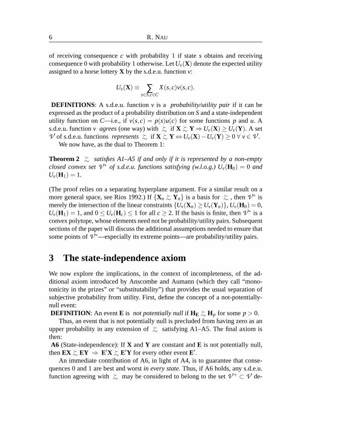
of receiving consequencec with probability 1 if states obtains and receivingconsequence 0 with probability 1 otherwise. LetUv(X) denote the expected utilityassigned to a horse lotteryX by the s.d.e.u. functionv:

Uv(X)≡ ∑s∈S,c∈C

X(s,c)v(s,c).

DEFINITIONS : A s.d.e.u. functionv is a probability/utility pair if it can beexpressed as the product of a probability distribution onSand a state-independentutility function onC—i.e., if v(s,c) = p(s)u(c) for some functionsp andu. As.d.e.u. functionv agrees(one way) with �∼ if X �∼ Y ⇒Uv(X)≥Uv(Y). A setV of s.d.e.u. functionsrepresents�∼ if X �∼ Y ⇔Uv(X)−Uv(Y)≥ 0 ∀ v∈ V .

We now have, as the dual to Theorem 1:

Theorem 2 �∼ satisfies A1–A5 if and only if it is represented by a non-emptyclosed convex setV ∗ of s.d.e.u. functions satisfying (w.l.o.g.) Uv(H0) = 0 andUv(H1) = 1.

(The proof relies on a separating hyperplane argument. For a similar result on amore general space, see Rios 1992.) If{Xn

�∼ Yn} is a basis for�∼ , thenV ∗ ismerely the intersection of the linear constraints{Uv(Xn)≥Uv(Yn)}, Uv(H0) = 0,Uv(H1) = 1, and 0≤Uv(Hc) ≤ 1 for all c≥ 2. If the basis is finite, thenV ∗ is aconvex polytope, whose elements need not be probability/utility pairs. Subsequentsections of the paper will discuss the additional assumptions needed to ensure thatsome points ofV ∗—especially its extreme points—are probability/utility pairs.

3 The state-independence axiom

We now explore the implications, in the context of incompleteness, of the ad-ditional axiom introduced by Anscombe and Aumann (which they call “mono-tonicity in the prizes” or “substitutability”) that provides the usual separation ofsubjective probability from utility. First, define the concept of a not-potentially-null event:DEFINITION : An eventE is not potentially nullif HE

�∼ Hp for somep > 0.Thus, an event that is not potentially null is precluded from having zero as an

upper probability in any extension of�∼ satisfying A1–A5. The final axiom isthen:A6 (State-independence): IfX andY are constant andE is not potentially null,

thenEX �∼ EY ⇒ E′X �∼ E′Y for every other eventE′.An immediate contribution of A6, in light of A4, is to guarantee that conse-

quences 0 and 1 are best and worstin every state. Thus, if A6 holds, any s.d.e.u.function agreeing with�∼ may be considered to belong to the setV + ⊂ V de-


fined by:

V + ≡ {v : 0 = v(s,0) ≤ v(s,c) ≤ v(s,1) ≤ 1 ∀ s∈ S, c≥ 2; ∑s∈S

v(s,1) = 1}.

Henceforth it will be assumed (arbitrarily but w.l.o.g.) that consequences 0 and1 have the same numerical utilities, namely 0 and 1, in every state as well asunconditionally. Then, regardless of whetherv is a probability/utility pair, define

pv(s)≡ v(s,1)

as “the” probability assigned to states by v, since it is the expected utility of ahorse lottery that yields a utility of 1 if states obtains and 0 otherwise. Corre-spondingly, ifE is an event,

pv(E)≡Uv(HE) = ∑s∈E

pv(s)

is the probability assigned toE by v. This method of defining probabilities (alsoused by Karni 1993) is based on the arbitrary assignment of equal utilities tothe best and worst outcomes in all states, hence it should not be interpreted asthe “true” probability of a hypothetical decision maker whose preferences arerepresented byv. The classic definitions of subjective probability given by Savage,Anscombe-Aumann, and others, are all afflicted with the same arbitrariness. Theintrinsic impossibility of inferring true probabilities from material preferencesis discussed by Kadane and Winkler (1988), Schervish et al. (1990), Karni andMongin (2000) and Nau (1995, 2002).)

Correspondingly, define:

uv(s,c)≡ v(s,c)/v(s,1) if v(s,1) > 0,

as the utility assigned to consequencec in states by v. This utility is state-independent ifv is a probability/utility pair, otherwise it is state-dependent. Inthese terms, the expected utility assigned toX by v can be rewritten as:

Uv(X) = ∑s

pv(s)∑c

uv(s,c)X(s,c).

We can now give a dual definition of conditional expected utility in terms ofv inthe obvious way:

Uv(X|E) = Uv(XE)/pv(E).

If the conditional expected utility ofX givenE is at leastuby our primal definition—i.e., if EX �∼ EHu—then dually we haveUv(X|E)≥ u for anyv agreeing with�∼and satisfyingpv(E) > 0, because for any agreeingv:

EX �∼ EHu⇒Uv(EX)≥Uv(EHu) = upv(E)⇔Uv(X|E)≥ u or else pv(E) = 0.

8 R. NAU

Another consequence of A6, in light of Theorem 1, is the property of stochas-tic dominance. In particular, ifX is obtained fromY by shifting probability massto consequence 1 from any other consequence, and/or from consequence 0 toany other consequence, in any state, thenX �∼ Y. To see this, note that A6 to-gether with A4 implies thatEsH1

�∼ EsHc andEsHc�∼ EsH0 for states and any

c > 1. HenceB∗ contains all vectors of the formEs(H1−Hc) andEs(Hc−H0).If X−Y can be expressed as a non-negative linear combination of these vectors,thenX−Y ∈B∗ and henceX �∼ Y. To make this result more precise, let the[ . ]min

(“minimum s.d.e.u.”) operation be defined onB as follows:

[B]min ≡ minv∈V +

Uv(B) = mins∈S

[B(s,1)+ ∑c≥2

min{0,B(s,c)}].

This quantity is the minimum possible state-dependent expected utility that couldbe assigned toB: it is achieved by assigning, within each state, a utility of 0 tothose consequencesc≥ 2 for whichB is positive and a utility of 1 to those conse-quencesc≥ 2 for whichB is negative, then assigning a subjective probability of 1to the state in which the conditional expected utility ofB is minimized. Stochasticdominance and the negative orthant inB can now be defined in a natural way:DEFINITIONS : X ≥∗ [>∗] Y (“X [strictly] dominatesY”) if [X−Y]min≥ [>] 0.The open negative orthantB− consists of thoseB that are strictly dominated bythe zero vector, i.e.,B− = {B ∈ B : 0 >∗ B}.

A6 in conjunction with A1–A5 then implies thatX ≥∗ [>∗] Y ⇒ X �∼ [�] Y.If preferences are complete (i.e., if for any horse lotteriesX andY, eitherX �∼ Yor Y �∼ X or both), then the primal representationB∗ is a half-space, the dualrepresentationV ∗ consists of a unique s.d.e.u. functionv∗, and axiom A6 re-quires the latter to be a probability/utility pair, which is the same result obtainedby Anscombe and Aumann (1963). (A6 implies thatUv∗(Hc|Es) = Uv∗(Hc) inde-pendent of the states.) In the absence of completeness, the contribution of A6 tothe separation of probability and utility is weaker, as summarized by:

Theorem 3 . �∼ satisfies A1–A6 only if it is represented by a nonempty closedconvex setV ∗∗ ⊆ V + of s.d.e.u. functions of which at least one element is aprobability/utility pair.

If {Xn�∼ Yn} is a basis for�∼ under axioms A1–A6, then any probability/utility

pair v that satisfiesUv(Xn) ≥Uv(Yn) for all n, v ∈ V +, belongs to the setV ∗∗.Apart from this fact, it is not easy to characterize the setV ∗∗ in terms of proba-bility/utility pairs, as will be illustrated in the sequel.


4 Strict vs. weak preference: an example

The results of the preceding section establish that a preference relation satisfyingA1–A6 is represented by a closed set of s.d.e.u. functions of which at least oneis a probability/utility pair. The closedness of the representing set is attributableto the use of weak preference as the behavioral primitive, together with a strongcontinuity assumption. In contrast, SSK use strict preference as the behavioralprimitive, together with a weaker continuity assumption, to explicitly allow forthe representation of incomplete preferences by open sets that may fail to containprobability/utility pairs.

The differences in these approaches are illustrated by an example of SSK(Example 4.1) comprising two states and three consequences, i.e.,S= {1,2} andC = {0,1,2}. Consequences 0 and 1 have state-independent utilities of 0 and 1 byassumption, so that a probability/utility pair is completely parameterized by theprobability assigned to state 1 and the utility assigned to consequence 2. Consider,then, the two probability/utility pairs(pi ,ui) in which p0(1) = 0.1 andp1(1) =0.3, andu0(2) = 0.1 andu1(2) = 0.4. Let v0 andv1 denote the correspondings.d.e.u. functions—i.e.,vi(s,c) = pi(s)ui(c) for i = 0,1. ThenUvi (X) denotes theexpected utility assigned to horse lotteryX by (pi ,ui). In particular,Uv0(H2) = 0.1andUv1(H2) = 0.4. Now let� be defined as the preference relation that satisfiesa weak Pareto condition with respect to these two probability/utility pairs—i.e.,X �Y⇔{Uv0(X) >Uv0(Y) and Uv1(X) >Uv1(Y)}. Any s.d.e.u. function that isa convex combination ofv0 andv1 also agrees with�, so the representing setV ∗∗

is the closed line segment whose endpoints arev0 andv1, but none of its interiorpoints are probability/utility pairs.

Next SSK extend� to obtain a new preference relation�′′ by imposing theadditional strict preferencesH0.4 �′′ H2 �′′ H0.1. The effect of this extensionis to chop off the two endpoints of the representing set of s.d.e.u. functions, sothat�′′ is represented by theopen line segment connectingv0 with v1. SSKpoint out that, although�′′ satisfies all their axioms, there is no agreeing prob-ability/utility pair for it, since the only two candidates have been deliberately ex-cluded. They proceed to axiomatize the concept of “almost state-independent”utilities, which agree with a strict preference relation and are “withinε” of beingstate-independent. Clearly,�′′ has an almost-state-independent representation,containing points arbitrarily close tov0 andv1.

In our framework, where weak preference is primitive, there is no way toimplement a constraint such asH2 � H0.1 (i.e., to chop offv0) except by assert-ing thatH2

�∼ H0.1+ε for a specific positiveε. And if this assertion is made, aninteresting thing happens: axiom A6 begins to nibble on thev0 end of the linesegment and continues nibbling until the representation collapses to thev1 end.To illustrate this process, let the non-zero elements of eachv be written out asv=({v(s,c)}) = (v(1,1),v(2,1);v(1,2),v(2,2)). Thus,v0 = (0.1,0.9;0.01,0.09) andv1 = (0.3,0.7;0.12,0.28). (Note that because these are probability/utility pairs,

10 R. NAU

the first two numbers in parentheses are the probabilities of states 1 and 2, andthe last two numbers are the same probabilities multiplied by the utility of con-sequence 2.) Next, let the line segment fromv0 to v1 be parameterized byvα ≡(1−α)v0 +αv1 for α ∈ (0,1). In these terms we obtain:

vα = (0.1+0.2α,0.9−0.2α;0.01+0.11α,0.09+0.19α),

whence:Uvα(H2) = vα(1,2)+vα(2,2) = 0.1+0.3α (4.1)

Uvα(H2|E1) =vα(1,2)vα(1,1)

=0.01+0.11α0.1+0.2α

(4.2)

Uvα(H2|E2) =vα(2,2)vα(2,1)

=0.09+0.19α0.9−0.2α

(4.3)

These are all monotone functions ofα for α between 0 and 1, and they all areequal to 0.1 atα = 0 and 0.4 atα = 1. However, for intermediate values ofα,(4.1) is greater than (4.3) and less than (4.2), and by invoking axiom A6, we canplay the last two off against each other. In particular, it follows from monotonicityof (4.2) that

α≥ α∗⇒Uvα(H2|E1)≥0.01+0.11α∗

0.1+0.2α∗, (4.4)

whereas it follows from monotonicity of (4.3) that

Uvα(H2|E2)≥ u∗⇒ α≥ 0.9u∗−0.090.2u∗+0.19

(4.5)

Let the setV ∗∗ representing the original relation� henceforth be parameterizedasV ∗∗ = {vα|α∈ [0,1]}. Suppose that we now increase the lower utility ofH2 byε = 0.01 by adding the preference assertionH2

�∼ H0.11 to the basis for�. Thisadditional assertion imposes the constraintUvα(H2) ≥ 0.11 for all vα agreeingwith the extended relation, thus excludingv0 as an agreeing s.d.e.u. function. Byapplication of A6, we may conclude thatUvα(H2|E2)≥ 0.11 as well. Substitutingu∗ = 0.11 in (4.5), it follows that the representing set must consist only of thosevαsatisfyingα≥ 0.042453. But now, substitutingα∗ = 0.042453 back into (4.4), wefind that it must also satisfyUvα(H2|E1) ≥ 0.135217. SinceE1 is not potentiallynull, A6 may be applied again to obtainUvα(H2)≥ 0.135217. Thus, if we take onebite out of the line segment by imposing the constraintUvα(H2) ≥ 0.11, we endup concluding that a larger biteUvα(H2)≥ 0.135217 may be taken. If we now re-peat the process by substitutingu∗ = 0.135217 in (4.5), we obtainα∗ = 0.146034,which yieldsUvα(H2|E1)≥ 0.201721 when substituted in (4.4). Successive itera-tions yieldu∗ values of 0.299288, 0.365247, 0.390144, 0.397381, 0.399317, andso on with rapid convergence to 0.4, which is realized (only) atv1. The continuityaxiom then allows us to assert thatH2

�∼ H0.4, which together with the originalconstraintH0.4

�∼H2, establishes that the utility of consequence 2 is precisely 0.4.


If instead we start at the other endpoint, adding the constraintH0.4−ε �∼ H2

for ε > 0, the collapse occurs to the 0.1 value. If both constraints are added—i.e.,if both endpoints are chopped off by finite margins, the entire interval is annihi-lated, yielding incoherence (a violation of A5). Hence, this example is unstablein the sense that anyfinite extension of the original preference relation leads toa collapse to one or the other of the original probability/utility pairs, or else toincoherence.

5 The need for stronger state-independence

The original preference relation in SSK’s example is represented by a set ofs.d.e.u. functions whose extreme points are both probability/utility pairs. In ourframework, if either of these points is excluded, then the intervening points mustbe excluded as well. Thus, in extending that relation, it is impossible to retain anyagreeing state-dependent utilities that are not convex combinations of agreeingstate-independent utilities. A second example shows that this is not always thecase under axioms A1–A6. In other words, a preference relation can satisfy theseaxioms and yet not be represented by utilities that are state-independent or even“almost” state-independent.

Let there be three states and three consequences, and letX denote the horselottery that satisfiesX(1,0) = X(2,2) = X(3,1) = 1. That is,X yields conse-quences 0, 2, and 1 with certainty in states 1, 2, and 3 respectively. Suppose thatall states are judged to have probability at least 0.1, andX is judged to have anunconditional expected utility of at least 0.5. Furthermore, a coin flip betweenXand{consequence 2 if state 1, otherwiseZ} is preferred to a coin flip betweenutility 0.5 and{utility 0.9 if state 1, otherwiseZ}, but also a coin flip betweenXand{utility 0.1 if state 2, otherwiseZ} is preferred to a coin flip between utility0.5 and{consequence 2 given state 2, otherwiseZ}. (The common alternativeZis arbitrary by Theorem 1.) Thus, the basis for�∼ is as follows:

HE�∼ H0.1 for E = E1,E2,E3, (5.1)

12

X +12

Z �∼12

H0.5 +12

Z, (5.2)

12

X +12(E1H2 +(1−E1)Z) �∼

12

H0.5 +12(E1H0.9 +(1−E1)Z), (5.3)

12

X +12(E2H0.1 +(1−E2)Z) �∼

12

H0.5 +12(E2H2 +(1−E2)Z), (5.4)

Notice that (5.3) and (5.4) are obtained from (5.2) by replacingZ by subjectivemixtures ofZ with different constant lotteries on the LHS and RHS. These lasttwo preferences imply that the lower bound on the expected utility ofX amongall probability/utility pairs agreeing with �∼ must be strictly greater than 0.5.

12 R. NAU

To understand this implication, note that under any s.d.e.u. function that agreeswith �∼ , the differences in expected utility between the LHS’s and RHS’s of(5.2), (5.3), and (5.4), must all be non-negative. Moreover, if the s.d.e.u. functionis a probability/utility pair, then in at least one of the two comparisons (5.3) and(5.4), the difference in expected utility between LHS and RHS must be strictlyless than it is in (5.2), a situation that occurs when consequence 2 has a utilitystrictly greater than 0.1 and/or strictly less than 0.9. If the difference in expectedutility between LHS and RHS is non-negative in all cases, then the difference cannever be zero in (5.2)—i.e.,X cannot have a lower expected utility as small as0.5. In fact, the minimum expected utility ofX among all probability/utility pairsagreeing with (5.1–5.4) is 0.564314.

The question is whether, by direct application of axioms A1–A6, we can inferthat the expected utility ofX is strictly greater than 0.5. The answer is: we cannot.The problem is that axiom A6 is useless here because of the common nonconstantterm X in (5.2)–(5.4). In order to apply A6, we must first find non-negative lin-ear combinations of the differences between the LHS’s and RHS’s of (5.1)–(5.4)that are conditionally constant—i.e., of the formEB, whereE is an event andBis constant across states. But the search for such conditionally constant terms isconstrained here by the presence of a common nonconstant termX−H0.5 in thedifferences between LHS’s and RHS’s of (5.2)–(5.4). Furthermore, in order forA6 to “bite,” B needs to have a negative lower expected utility when conditionedon some other eventE′. The effect of applying A6 will then be to raise this lowerexpected utility to zero, which shrinks the set of s.d.e.u. functions representing�∼ . In the example, the few conditionally-constant lottery differencesEB that

can be constructed from (5.1)–(5.4) all turn out to satisfyB ≥∗ 0, which is un-informative. The lower expected utility ofX therefore remains at 0.5 despite thefact that this value is not realized,or even closely approached, by any probabil-ity/utility pair agreeing with �∼ .

This example shows that when preferences are incomplete, axiom A6 is insuf-ficient to guarantee that they are represented by a set of probability/utility pairs(or their convex hull). Evidently, an additional state-independence condition isneeded, such as:A7 (Stochastic substitution): If

αX +(1−α)(EX′+(1−E)Z) �∼ αY +(1−α)(EY′+(1−E)Z)

for someα ∈ (0,1) whereX′ andY′ andZ are constant lotteries andE is notpotentially null, then

αX +(1−α)(pX′+(1− p)Z) �∼ αY +(1−α)(pY′+(1− p)Z)

for somep∈ (0,1].In other words, the subjective mixtures of the constant lotteriesX′ andY′ with

Z can be replaced with objective mixturesagainst the backgroundof a compari-


son between the nonconstant lotteriesX andY. In terms of the primal representa-tion B∗, this assumption means that ifB+EB′ ∈ B∗, whereB′ is constant acrossstates andE is not potentially null, thenB+ pB′ ∈ B∗ for somep > 0. (By com-parison,A2 andA6 imply only that this substitution may be performed in the non-stochastic caseB = 0.) Note that if a collection of preferences{Xn

�∼ Yn} satisfiesA1–A6, then the imposition of A7 cannot produce a contradiction. A1–A6 requirethe existence of at least one probability/utility pair agreeing with{Xn

�∼ Yn}, andany probability/utility pair that agrees with the original preferences will also agreewith any new preferences generated from them by A7.

The new axiomdoesaffect the counterexample discussed above. (5.3) and(5.4) can now be replaced by

12

X +12(pH2 +(1− p)Z) �∼

12

H0.5 +12(pH0.9 +(1− p)Z),

12

X +12(p′H0.1 +(1− p′)Z) �∼

12

H0.5 +12(p′H2 +(1− p′)Z),

for somep, p′ > 0. A mixture of these two comparisons in a ratio ofp′ to p yields:

12

X +12(αH0.1 +αH2 +(1−2α)Z) �∼

12

H0.5 +12(αH0.9 +αH2 +(1−2α)Z),

whereα = pp′/(p+ p′). The LHS must have greater-or-equal expected utilitythan the RHS, which (because of theH0.1 term on the left and theH0.9 term onthe right, and cancellation of the common termsH2 andZ) means thatX musthave strictly greater expected utility than 0.5.

The main result, which generalizes this example, can now be stated as:

Theorem 4 �∼ satisfies A1–A7 if and only if it is represented by a nonempty setV ∗∗∗ of s.d.e.u. functions that is the convex hull of a set of probability/utility pairs.

If {Xn�∼ Yn} is a basis for�∼ under A1–A7, thenV ∗∗∗ is merely the convex hull

of the set of probability/utility pairs that satisfy{Uv(Xn)≥Uv(Yn)}. If the basis isfinite, the construction ofV ∗∗∗ can be carried out as follows. First, form the con-vex polyhedron defined by the constraints{Uv(Xn) ≥Uv(Yn)}, v ∈ V +. Next,take the intersection of this polyhedron with the nonconvex surface consisting ofall probability/utility pairs. (If the latter intersection is empty, the preferences donot satisfy A1–A7: they are incoherent.) Finally, take the convex hull of whatremains: this is the setV ∗∗∗.

14 R. NAU

6 Discussion

It has been shown that, in order to obtain a convenient representation of incom-plete preferences by sets of probability/utility pairs, it does not suffice merely todelete the completeness axiom from the standard axiomatic framework of Anscombeand Aumann. This finding is not due to technical problems with limits or nullevents, but rather to a fundamental weakness of the traditional state-independenceaxiom in the absence of completeness. Our approach is to introduce an additionalstate-independence postulate (A7) that has “bite” in the absence of completeness.SSK follow a different approach in their axiomatization of incomplete strict pref-erences. Instead of directly strengthening the state-independence property, they“fill in the missing preferences” by indirect reasoning, namely, they assume thepreference relation has the property that¬(X �∼ Y)⇒ Y � X, where “¬” standsfor “it is precluded that,” meaning that there is no extension of�∼ satisfyingthe other axioms in whichX �∼ Y (p. 2204 ff.). SSK’s assumption requires thatwherever a weak preference is precluded, the opposite strict preference must beaffirmed. In our framework, this property of�∼ is not implied by axioms A1–A6,hence it amounts to an additional axiom of rationality. The lack of this property isillustrated by the example of the preceding section, in which it is precluded thatHu

�∼ X for any u < 0.5643...., yet it is not implied by A1–A6 thatX � Hu forany u > 0.5. If the “axiom” of indirect reasoning is added to A1–A6, in lieu ofA7, the representation of Theorem 4 follows immediately from Theorem 3.

APPENDIX

Proof of Theorem 1: Suppose thatX − Y ∝ X′ − Y′, i.e., α(X − Y) = (1−α)(X′−Y′) for someα ∈ (0,1), whereX,Y,X′,Y′ are horse lotteries. Then, bythe mixture-independence axiom,X �∼ Y ⇔ αX +(1−α)X′ �∼ αY +(1−α)X′ =αX +(1−α)Y′ ⇔ X′ �∼ Y′, establishing that there is a collection of vectorsB∗

such thatB ∈ B∗ ⇒ αB ∈ B∗ ∀ α > 0 andX �∼ Y ⇔ X −Y ∈ B∗. Mixture-independence and transitivity together imply that ifX �∼ Y and X′ �∼ Y′, thenαX +(1−α)X′ �∼ αY +(1−α)Y′, establishing thatB∗ is convex. The best/worstaxiom establishes thatB∗ is non-empty (in particular, it includesHc−H0 andH1−Hc for c > 1), but coherence requires that it not be the whole space (in par-ticular, it excludesH0−H1), and the continuity axiom implies that it is closed.

Proof of Theorem 2: By duality, a convex coneB∗ is characterized by a convexsetV ∗ of vectors inB such thatB ∈ B∗ if and only if Uv(B) ≡ vTB ≥ 0 for allv∈ V ∗, and coherence requires thatUv(H1−H0) > 0 for all v∈ V ∗. Since theelements ofB∗ are differences between pairs of horse lotteries, their componentssum to zero within states. Hence,Uv(B) ≥ 0⇔ Uv′(B) ≥ 0 wherev′ = αv+ β


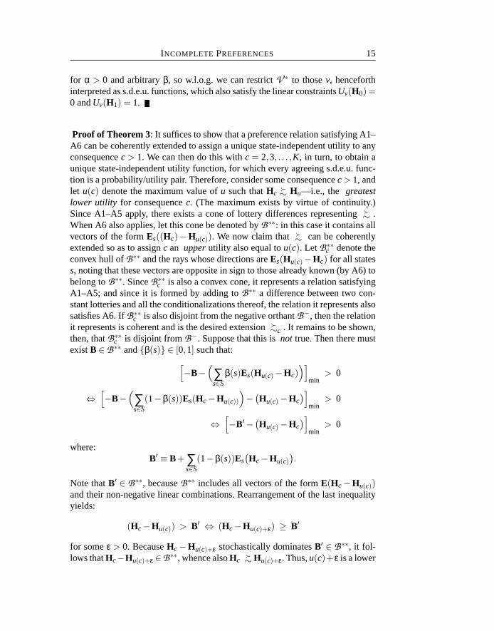
for α > 0 and arbitraryβ, so w.l.o.g. we can restrictV ∗ to thosev, henceforthinterpreted as s.d.e.u. functions, which also satisfy the linear constraintsUv(H0) =0 andUv(H1) = 1.

Proof of Theorem 3: It suffices to show that a preference relation satisfying A1–A6 can be coherently extended to assign a unique state-independent utility to anyconsequencec > 1. We can then do this withc = 2,3, . . . ,K, in turn, to obtain aunique state-independent utility function, for which every agreeing s.d.e.u. func-tion is a probability/utility pair. Therefore, consider some consequencec> 1, andlet u(c) denote the maximum value ofu such thatHc

�∼ Hu—i.e., the greatestlower utility for consequencec. (The maximum exists by virtue of continuity.)Since A1–A5 apply, there exists a cone of lottery differences representing�∼ .When A6 also applies, let this cone be denoted byB∗∗: in this case it contains allvectors of the formEs((Hc)−Hu(c)). We now claim that�∼ can be coherentlyextended so as to assignc an upperutility also equal tou(c). Let B∗∗

c denote theconvex hull ofB∗∗ and the rays whose directions areEs(Hu(c)−Hc) for all statess, noting that these vectors are opposite in sign to those already known (by A6) tobelong toB∗∗. SinceB∗∗

c is also a convex cone, it represents a relation satisfyingA1–A5; and since it is formed by adding toB∗∗ a difference between two con-stant lotteries and all the conditionalizations thereof, the relation it represents alsosatisfies A6. IfB∗∗

c is also disjoint from the negative orthantB−, then the relationit represents is coherent and is the desired extension�∼c . It remains to be shown,then, thatB∗∗

c is disjoint fromB−. Suppose that this isnot true. Then there mustexistB ∈ B∗∗ and{β(s)} ∈ [0,1] such that:[

−B−(∑s∈S

β(s)Es(Hu(c)−Hc))]

min> 0

⇔[−B−

(∑s∈S

(1−β(s))Es(Hc−Hu(c))

)−

(Hu(c)−Hc

)]min

> 0

⇔[−B′−

(Hu(c)−Hc

)]min

> 0

where:B′ ≡ B+ ∑

s∈S

(1−β(s))Es(Hc−Hu(c)

).

Note thatB′ ∈ B∗∗, becauseB∗∗ includes all vectors of the formE(Hc−Hu(c))and their non-negative linear combinations. Rearrangement of the last inequalityyields:

(Hc−Hu(c)) > B′ ⇔ (Hc−Hu(c)+ε) ≥ B′

for someε > 0. BecauseHc−Hu(c)+ε stochastically dominatesB′ ∈ B∗∗, it fol-lows thatHc−Hu(c)+ε ∈B∗∗, whence alsoHc

�∼Hu(c)+ε. Thus,u(c)+ε is a lower

16 R. NAU

utility for c, contradicting the assumption thatu(c) was the greatest lower utilityfor c under the relation�∼ , establishing that the extended relation is coherent.

Proof of Theorem 4: The earlier results (based on A1–A6 only) establish that�∼ is represented by a convex cone of horse-lottery-differences and dually by a

convex set of expected utility functions containing at least one probability/utilitypair. When A7 also holds, let these sets be denoted byB∗∗∗ andV ∗∗∗, respectively.It remains to be shown thatV ∗∗∗ is the convex hull of a set of probability/utilitypairs, which means that for any horse lotteriesX,Y, the minimum ofUv(X)−Uv(Y) over allv∈ V ∗∗∗ is achieved at somev which is a probability/utility pair.Suppose thatd = minv∈V ∗∗∗Uv(X)−Uv(Y). SinceUv(H0) = 0 andUv(Hu) = u,it follows thatd is the maximum value ofu for which

Uv(12

X +12

H0)≥Uv(12

Y +12

Hu) (7.1)

for all v∈ V ∗∗∗, or equivalently the maximum value ofu for which

12

X +12

H0�∼

12

Y +12

Hu,

or equivalently the maximum value ofu for which

X +H0−Y−Hu ∈ B∗∗∗. (7.2)

To prove the result, it must be shown that there is a probability/utility pair forwhich (7.1) holds with equality. For this purpose, it will suffice to prove that�∼has a coherent extension, denoted�∼d , in which the reverse preference also holds,i.e.:

12

Y +12

Hd�∼d

12

X +12

H0, (7.3)

If V ∗∗∗d denotes the set of s.d.e.u. functions representing�∼d , then (7.1) must

hold with equality for allv∈V ∗∗∗d , of which, by Theorem 3, at least one must be a

probability/utility pair. We must still show that the coherent extension�∼d exists.The minimal extension of�∼ which satisfies (7.3) has a primal representationwhich is constructed in the following way. First, add to the convex coneB∗∗∗ theray whose direction isY + Hd −X −H0, noting that this direction is oppositeto the vector on the LHS of (7.2) foru = d, which is an extreme element ofB∗∗∗. Then apply A1–A3, which convexifies the set, yielding an expanded cone.Next apply A6, which means to (i) determine which new vectors of the formEB,whereE is not potentially null andB is constant across states, are in the expandedcone; (ii) then add all other vectors of the formE′B, whereE′ is another event;and (iii) take the convex hull again. (Technically, A7 must also be applied to


the extended collection of preferences in order to complete the characterization of�∼d . However, as noted above, the application of A7 following A6 does not affect

coherence. Therefore, in order to establish that the extended relation is coherent,it suffices to consider the situation following the application of A6.)

It must now be shown that the expanded cone remains disjoint from the neg-ative orthantB−. First, note that adding toB∗∗∗ the ray whose direction isY +Hd−X−H0 and then taking the convex hull cannot by itself produce incoher-ence, becauseB∗∗∗ encloses the positive orthant, and the ray whose direction isY + Hd−X−H0 lies in a supporting hyperplane toB∗∗∗ because it is the op-posite of an extreme element ofB∗∗∗. The question, then, is whether any newpreferences generated between conditionally-constant lotteries will produce in-coherence when propagated by A6 to other conditioning events. Observe that,if EB is in the expanded cone but not the original cone, whereE is not poten-tially null andB is constant across states, thenX +H0−Y−Hd +EB must havebeen in the original cone. Let{EiBi , i = 1,2, . . .} denote the set of allEB pairsof this form. That is,Ei is not potentially null,Bi is constant across states, andX + H0−Y−Hd + EiBi ∈ B∗∗∗ for all i. The result of applying A6 is that allvectors of the formE′Bi are added to the cone and convexified. Suppose that thefinal cone so obtained contains a vector lying in the negative orthant. Since it wasproduced by propagating constant vectors across all possible conditioning events,including the certain event, we may assume w.l.o.g. that the negative vector isconstant across states, and that it can be represented as∑i=0,1,... αiBi , whereB0 isa (constant) element of the original cone

B∗∗∗, {Bi} are the new constant vectors that were added by application of A6,andαi ≥ 0 for all i. Finally, invoke the fact that the original preference relation�∼ satisfies A7 as well as A1–A6. Then there existpi > 0 such that

X +H0−Y−Hd + piBi ∈ B∗∗∗

for i = 1,2, . . . . This also is true fori = 0 since bothX + H0−Y−Hd andB0

are elements ofB∗∗∗. Multiplying through byαi/pi , summing, and invoking theconvexity ofB∗∗∗, yields:

X +H0−Y−Hd +( ∑i=0,1,...

αi/pi)−1 ∑i=0,1,...

αiBi ∈ B∗∗∗

Since∑i=0,1,... αiBi is a negative vector, it must be true thatX + H0−Y−Hu ∈B∗∗∗ for someu> d, contradicting the assumption thatd was the maximum valueof u for whichX +H0−Y−Hu ∈ B∗∗∗.

18 R. NAU

Mathematical programs for the example in section 5: The original basis vec-tors forB∗∗ in this example are as follows:

B1 = E1(H2−H0), B2 = E2(H2−H0), B3 = E3(H2−H0),B4 = E1(H1−H2), B5 = E2(H1−H2), B6 = E6(H1−H2),

B7 = HE1−H0.1, B8 = HE2−H0.1, B9 = HE3−H0.1,

B10 = X−H0.5

B11 = X−H0.5 +E1(H2−H0.9)B12 = X−H0.5 +E2(H0.1−H2)

Note thatB1, . . . ,B6 are the contribution of axioms A4 and A6 together;B7,B8, andB9 are the differences between LHS and RHS of (5.1) forE = E1,E2,E3;andB10, B11, andB12 are the differences between LHS and RHS of (5.2)–(5.4),after dropping the multiplicative constants1

2 and cancelling the commonZ terms.Axioms A1–A4 establish that the coneB∗∗ representing this preference re-

lation minimally consists of the convex hull of the rays whose directions areB1, . . . ,B12. The question is whether axiom A6 enlarges this cone. To prove thatit does not, we can solve a series of linear programs to show that there are no non-negative linear combinations ofB1, . . . ,B12 which are of the formEB, whereE isan event andB is constant, and which are nontrivial in the sense that[B]min < 0.(Recall that[B]min is defined as the minimum possible state-dependent expectedutility assignable toB. If this is not negative, thenB is simply a linear combina-tion of B1, . . . ,B6, as isE′B for any other eventE′, so the application of A6 to thisB does not enlarge the cone.)

If B is constant, then[B]min is the minimum ofB(s,1) andB(s,1)+B(s,2) forany events. To formulate this problem as a linear program, we must separatelyminimize each of these two quantities over all non-negativeα1, . . . ,α12 such that

∑i

αiBi = EB,

B(1,c) = B(2,c) = B(3,c), c = 0,1,2,

for every possible conditioning eventE. There are seven distinct events that aresubsets ofSin this case, namely{E1,E2,E3},{E1,E2},{E1,E3},{E2,E3},{E1},{E2}, and{E3}. Altogether, we must solve 14 linear programs (2 objective func-tions× 7 conditioning events) to see whether any has a negative optimal objec-tive value. As it happens, none does. Hence, the coneB∗∗ is merely the set ofnon-negative linear combinations ofB1, . . . ,B12. To establish the lower expectedutility for X that can be deduced from A1–A6, we can solve the primal inferenceproblem, namely find the maximum value ofu for which

∑i

αiBi = X−Hu


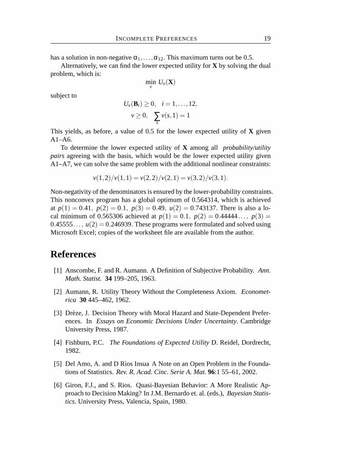
has a solution in non-negativeα1, . . . ,α12. This maximum turns out be 0.5.Alternatively, we can find the lower expected utility forX by solving the dual

problem, which is:min

vUv(X)

subject toUv(Bi)≥ 0, i = 1, . . . ,12,

v≥ 0, ∑s

v(s,1) = 1

This yields, as before, a value of 0.5 for the lower expected utility ofX givenA1–A6.

To determine the lower expected utility ofX among all probability/utilitypairs agreeing with the basis, which would be the lower expected utility givenA1–A7, we can solve the same problem with the additional nonlinear constraints:

v(1,2)/v(1,1) = v(2,2)/v(2,1) = v(3,2)/v(3,1).

Non-negativity of the denominators is ensured by the lower-probability constraints.This nonconvex program has a global optimum of 0.564314, which is achievedat p(1) = 0.41, p(2) = 0.1, p(3) = 0.49, u(2) = 0.743137. There is also a lo-cal minimum of 0.565306 achieved atp(1) = 0.1, p(2) = 0.44444. . . , p(3) =0.45555. . . , u(2) = 0.246939. These programs were formulated and solved usingMicrosoft Excel; copies of the worksheet file are available from the author.

References

[1] Anscombe, F. and R. Aumann. A Definition of Subjective Probability.Ann.Math. Statist.34199–205, 1963.

[2] Aumann, R. Utility Theory Without the Completeness Axiom.Economet-rica 30445–462, 1962.

[3] Dreze, J. Decision Theory with Moral Hazard and State-Dependent Prefer-ences. In Essays on Economic Decisions Under Uncertainty. CambridgeUniversity Press, 1987.

[4] Fishburn, P.C. The Foundations of Expected UtilityD. Reidel, Dordrecht,1982.

[5] Del Amo, A. and D Rios Insua A Note on an Open Problem in the Founda-tions of Statistics.Rev. R. Acad. Cinc. Serie A. Mat.96:1 55–61, 2002.

[6] Giron, F.J., and S. Rios. Quasi-Bayesian Behavior: A More Realistic Ap-proach to Decision Making? In J.M. Bernardo et. al. (eds.),Bayesian Statis-tics. University Press, Valencia, Spain, 1980.

20 R. NAU

[7] Kadane, J.B. and R.L. Winkler. Separating Probability Elicitation from Util-ities. J. Amer. Statist. Assoc.83:402 357–363, 1988.

[8] Karni, E. and P. Mongin. On the Determination of Subjective Probability byChoices.Management Science46233–248, 2000.

[9] Karni, E., Schmeidler, D. and K. Vind. On State-Dependent Preferences andSubjective Probabilities.Econometrica511021–1031, 1983.

[10] Karni, E. Decision Making Under Uncertainty: The Case of State-Dependent Preferences. Harvard University Press, Cambridge, 1985.

[11] Karni, E. A Definition of Subjective Probabilities with State-DependentPreferences.Econometrica61187–198, 1993.

[12] Luce, R.D. and H. Raiffa.Games and Decisions: Introduction and CriticalSurvey.Wiley, New York, 1957.

[13] Moskowitz, Preckel and Yang. Decision Analysis with Incomplete Proba-bility and Utility Information. Operns. Res41864–879, 1993.

[14] Nau, R. Indeterminate Probabilities on Finite Sets.Ann. Statist. 20:41737–1767, 1992.

[15] Nau, R. Coherent Decision Analysis with Inseparable Probabilities and Util-ities. J. Risk and Uncertainty1071–91, 1995.

[16] Nau, R. De Finetti Was Right: Probability Does Not Exist.Theory andDecision5189–124, 2002.

[17] Rios Insua, D. Sensitivity Analysis in Multiobjective Decision Making.Springer-Verlag, 1990.

[18] Rios Insua, D. On the Foundations of Decision Making under Partial Infor-mation. Theory and Decision3383–100, 1992.

[19] Schervish, M.J, T. E. Seidenfeld and J.B. Kadane. State-Dependent Utilities.J. Amer. Statist. Assoc.85:411 840–847, 1990.

[20] Seidenfeld, T., M. J. Schervish and J. B. Kadane. Decisions Without Order-ing. In W. Sieg (ed.)Acting and Reflecting, Reidel, Dordrecht, 1990.

[21] Seidenfeld, T.E., M.J. Schervish and J.B. Kadane. A Representation of Par-tially Ordered Preferences.Ann. Statist.232168–2174, 1995.

[22] Smith, C.A.B. Consistency in Statistical Inference and Decision.J. Roy.Stat. Soc. B231–25, 1961.


[23] Staum, J. Pricing and Hedging in Incomplete Markets: Fundamental Theo-rems and Robust Utility Maximization.Math. Finance, forthcoming.

[24] Suppes, P. The Measurement of Belief.J. Roy. Stat. Soc. B36 160–175,1974.

[25] Walley, P. Statistical Reasoning with Imprecise Probabilities. Chapmanand Hall, London, 1991.

[26] Williams, P.M. Indeterminate Probabilities. In M. Przełecki, K. Szaniawski,and R. Wojcicki (eds.), Formal Methods in the Methodology of EmpiricalSciencesOssolineum and D. Reidel, Dordecht, Holland 229–246, 1976.

FUQUA SCHOOL OFBUSINESS

DUKE UNIVERSITY

DURHAM , NC 27708-0120 [email protected]

the shape of incomplete preferences1

Documents