HYPOTHESIS AND THEORY ARTICLEpublished: 23 August 2013

doi: 10.3389/fncom.2013.00117

The situated HKB model: how sensorimotor spatialcoupling can alter oscillatory brain dynamicsMiguel Aguilera 1*, Manuel G. Bedia1, Bruno A. Santos2,3 and Xabier E. Barandiaran 4

1 Department of Computer Science and Engineering Systems, University of Zaragoza, Zaragoza, Spain2 Department of Informatics, CCNR, University of Sussex, Brighton, UK3 Laboratory of Intelligent Systems, Cefet-MG, Belo Horizonte, Brazil4 Department of Philosophy, IAS-Research Centre for Life, Mind and Society, University School of Social Work, UPV/EHU University of the Basque Country, San

Sebastián, Spain

Edited by:

Rava A. Da Silveira, Ecole NormaleSupérieure, France

Reviewed by:

Tatyana Sharpee, Salk Institute forBiological Studies, USAEmili Balaguer-Ballester,Bournemouth University, UK

*Correspondence:

Miguel Aguilera, Departamento deInformática e Ingeniería deSistemas, Universidad de Zaragoza,Edificio Ada Byron, C/ María deLuna, 1, 50018 Zaragoza, Spaine-mail: miguel.academic@maguilera.net

Despite the increase of both dynamic and embodied/situated approaches in cognitivescience, there is still little research on how coordination dynamics under a closedsensorimotor loop might induce qualitatively different patterns of neural oscillationscompared to those found in isolated systems. We take as a departure point theHaken-Kelso-Bunz (HKB) model, a generic model for dynamic coordination between twooscillatory components, which has proven useful for a vast range of applications incognitive science and whose dynamical properties are well understood. In order to explorethe properties of this model under closed sensorimotor conditions we present what wecall the situated HKB model: a robotic model that performs a gradient climbing task andwhose “brain” is modeled by the HKB equation. We solve the differential equations thatdefine the agent-environment coupling for increasing values of the agent’s sensitivity(sensor gain), finding different behavioral strategies. These results are compared with twodifferent models: a decoupled HKB with no sensory input and a passively-coupled HKBthat is also decoupled but receives a structured input generated by a situated agent. Wecan precisely quantify and qualitatively describe how the properties of the system, whenstudied in coupled conditions, radically change in a manner that cannot be deduced fromthe decoupled HKB models alone. We also present the notion of neurodynamic signatureas the dynamic pattern that correlates with a specific behavior and we show how only asituated agent can display this signature compared to an agent that simply receives theexact same sensory input. To our knowledge, this is the first analytical solution of the HKBequation in a sensorimotor loop and qualitative and quantitative analytic comparison ofspatially coupled vs. decoupled oscillatory controllers. Finally, we discuss the limitationsand possible generalization of our model to contemporary neuroscience and philosophy ofmind.

Keywords: HKB model, situated hkb model, embodied cognition, sensorimotor coupling, coordination dynamics,

dynamical analysis, neurodynamics

1. DYNAMICISM AND SITUATEDNESS IN COGNITIVE(NEURO)SCIENCE

Cognitive science (and cognitive neuroscience in particular) iswitnessing an increasing success of dynamical systems models,often displacing computational and representational conceptionsof cognitive functioning. This change is not new, it can be tracedback to early cybernetics (Ashby, 1952; Walter, 1963; Powers,1973), neuroscience (Holst, 1973) phenomenology (Merleau-Ponty, 1942), and pragmatism (Dewey, 1896, 1922). But it wasnot until the 1990’s that a strong paradigmatic shift began totake place in the fields of autonomous robotics (Brooks, 1991),adaptive behavior (Beer, 1990, 1997), coordination dynamics(Kelso, 1995), neuroscience (Skarda and Freeman, 1987), devel-opmental psychology (Thelen and Smith, 1994), and philoso-phy of mind (Port and Gelder, 1995; Clark, 1997). Dynamicistapproaches have had two central contributions: (a) that cognitive

mechanisms (neural or otherwise) could be better effectivelymodeled and understood in terms of dynamical systems (Haken,1978; Kelso, 1995; Freeman, 2001) instead of symbolic represen-tational algorithms (e.g., Fodor, 1983; Pinker, 1997; Carruthers,2006) and (b) that cognitive behavior could emerge out of recur-rent sensorimotor loops in a self-organized manner, without theneed for explicit encoding and planning on the side of the agent.And yet the relationship between both contributions remains rel-atively under-explored: how does the self-organization of behav-ior change the dynamical properties of brains? What is lost whenwe study brain dynamics in isolation from the sensorimotor loopsthey are naturally embedded in?

Some of the latest progress at both mechanistic (neurody-namic) and behavioral levels of dynamic modeling is relatedto oscillatory dynamics. Interactions between oscillatory com-ponents (neurons, brain regions, limbs or humans interacting

Frontiers in Computational Neuroscience www.frontiersin.org August 2013 | Volume 7 | Article 117 | 1

COMPUTATIONAL NEUROSCIENCE

Aguilera et al. The situated HKB model

with each other) are studied in terms of synchronization andphase-difference at various scales where macroscopic variablesprovide indexes of emergent collective behavior (Strogatz, 2004;Buzsaki, 2006). Oscillations are ubiquitous in nature, from plan-etary motion to circadian rhythms (Pittendrigh, 1960), frompredator-prey populations (Lotka, 1920) to chemical dynamics(Kuramoto, 1984). Oscillatory activity is also present at dif-ferent levels of the nervous system (Freeman, 2001). At theindividual neural level, neurons undergo cyclic alterations ontheir membrane potential following different dynamical regimesdepending on the cell properties (Izhikevich, 2006). At higher lev-els, global oscillations are observed as a collective phenomenongenerated by groups of neural cells that fire synchronously[entrained by pacemaker cells or as a result of recurrent networkactivity with inhibitory-excitatory connections (Buzsaki, 2006)].Different aspects of large-scale brain oscillatory activity (e.g., self-organization of emergent patterns, synchronization and oscilla-tory rhythms) have become a common explanatory resource inbehavioral and cognitive neuroscience. Some of the phenom-ena that have gained explanatory benefit from this approachinclude the binding of the different perceived features of an object(Phillips and Singer, 1997), the representation of position infor-mation in navigation tasks (O’Keefe and Recce, 1993), attention(Deco and Thiele, 2009), memory (Jensen et al., 2007), and con-scious experience (Crick and Koch, 1990; Engel et al., 1999; Varelaet al., 2001).

Despite the significant progress recently achieved by investi-gating oscillatory dynamics in cognitive neuroscience, existingtheoretical frameworks and models are mostly developed with-out taking into account sensorimotor dynamics and, even appearlimited in the establishment of oscillatory correlations after agiven stimulus onset. Computational models are generally builtwithout considering the body and the environment and oftenassuming a representational theory of brain function (that is, theyassume that the main job of the brain is to create a representationor model of the environment, and focus on neuronal mecha-nisms capable of supporting the processing of such a model). As aresult, the focus of oscillatory brain dynamics is often centered onthose aspects of oscillatory activity that might carry informationwithin the brain, without considering the coupled brain-body-environment dynamics. This is even true for non-representationalapproaches to cognition that acknowledge the theoretical rele-vance of situated cognition but conduct most of their studies insearch for cognitive correlates in oscillatory brain activity leav-ing aside the potential effects of the sensorimotor coupling (e.g.,Skarda and Freeman, 1987; Varela et al., 2001).

Sensorimotor coordination implies more than the state-ment that sensory input will, through its influence on brainoscillations, create an action that, in turn, will produce achange that leads to a new perceptual state. The central claimof situated approaches to cognitive behavior is that the agent-environment coupling shapes brain dynamics in a mannerthat is essential to behavioral or cognitive functionality (Steels,1990; Chiel and Beer, 1997; Clark, 1997). In other words,macroscopic functional behavior (e.g., intentional grasping orperception) emerges from microscopic sensorimotor dynam-ics (e.g., proprioceptive and visual feedback in grasping or

saccadic movements in visual perception). Thus, cognitivebehavior is not the result of a linear computational sequenceinvolving sensation→perceptive-categorization→planning→action-selection→motor-execution, but the result of recurrentsensorimotor and brain oscillatory coordination at multiplescales. The central role that sensorimotor dynamics play incognitive phenomenology has been recently highlighted bySensorimotor Contingency Theory (O’Regan and Noë, 2001),defending that what is constitutive of perceptual awareness (and,it could be argued, other cognitive states) is not a specific internalstate of an agent, but the structure of sensorimotor contingencies.To perceive is to act in a specific manner that brings forth thestructure of sensory changes in relation to the activity of theagent. To see or to perceive is something that is done and lies onthe very sensorimotor coupled dynamics of an agent.

Filling the gap between the study of brain oscillatory activ-ity and the situated sensorimotor dynamics is essential if wewant to understand the nature of cognition. However, despitethe repeated emphasis on the importance of sensorimotor cou-pling for neurodynamic approaches 1 (Kelso, 1995; Freeman,2001; Dreyfus, 2007; Chemero, 2009), there are very few exam-ples of these types of models that exploit sensorimotor couplingand almost none for oscillatory models (some recent exceptionsinclude Moioli et al., 2010; Santos et al., 2011). Current under-standing of brain oscillatory dynamics is limited to “passive”conditions. The dynamical properties of oscillatory networks(even when studied within the context of behavioral or cognitiveneuroscience, see Strogatz, 2004) are deduced from mathematicaland computational models that have constant or no input at all,and the effect of sensorimotor or situated dynamics on the oscilla-tory properties of such networks is rarely considered. The goal ofthis paper is to make a theoretical contribution in the direction ofexplicitly quantifying the difference between dynamics that resultfrom isolated vs. situated oscillatory controllers, and those thatresult from actively vs. passively coupled systems.

We have chosen the Haken-Kelso-Bunz (HKB) model as aparadigmatic example of oscillatory dynamics and behavior toaddress these questions. There are a number of good reasons tochoose the HKB model. On the one hand the HKB model is sim-ple enough to be treated analytically, on the other hand it has beenused both to model behavioral phenomena and to model braindynamics (see next section for details). Finally, to our knowl-edge, no variation of the HKB model exists that has used it asa controller of a sensorimotor system and no analytic study existsof a comparison between the dynamics of the HKB studied inisolation (with a parametric analysis) and its dynamics under sen-sorimotor loop conditions (with few exceptions as, for instance,Kelso et al., 2009).

The structure of the paper is as follows: (1) first we intro-duce the well known HKB model and the coordination dynamicsparadigm; (2) next, we characterize the notion of dynamicallycoupled and spatially situated system and present a novel exten-sion of the HKB model with sensorimotor embodiment that we

1By neurodynamic approaches we refer to dynamical system approaches tothe understanding of neural activity (Gelder, 1998; Freeman, 2001; Buzsaki,2006, etc.).

Frontiers in Computational Neuroscience www.frontiersin.org August 2013 | Volume 7 | Article 117 | 2

Aguilera et al. The situated HKB model

call the situated HKB model; (3) then, we analytically solve a par-ticular case of the situated HKB model performing a gradientclimbing task in a 2D environment. Later, (4) we compare theobtained dynamics of the coupled system with the dynamics ofa decoupled HKB and with a passively-coupled HKB model foran equivalent parametric analysis. Qualitative changes betweenthe eigenvalues describing the three HKB-system dynamics willbe identified, as well as experimental measures characterizing thetransformation of the complete phase space of the agent pro-duced by sensorimotor coupling. Finally, (5) we discuss someimplications for the study of oscillatory brain dynamics.

2. THE HKB MODEL AND THE “COORDINATION DYNAMICS”PARADIGM

One of the most important current conceptual and modelingframeworks that might integrate oscillatory dynamics and senso-rimotor coupling is Scott Kelso’s coordination dynamics paradigm(Kelso, 1995) and the different variations of the HKB model(Haken et al., 1985) that have been used to study coordinationphenomena. Coordination dynamics is a mathematical and con-ceptual framework used to investigate coordinated patterns inbrain dynamics and behavior. It was proposed and developedby Kelso (1995), and is based on Haken’s work on synergetics(Haken, 1978). It combines experiments and formal theoreticalmodels to study how the components of a system interact andproduce coherent coordination patterns.

The HKB model has been the driving example for the coor-dination dynamics paradigm, describing the behavior of twonon-linearly coupled oscillators. The model was originally formu-lated in 1985 to explain experimental observations in the relativephase dynamics of bimanual coordination (Haken et al., 1985)but it has been shown to capture the coordination dynamicsof different behavioral (Kelso, 1995), neural (Jirsa et al., 1994),and social (Oullier and Kelso, 2009) phenomena as well. Usingthe language of synergetics (order parameters, control param-eters, instability, etc., see Haken, 1978), the HKB describesa simple non-linearly coupled dynamical system that capturesthe self-organized behavior of two generic coordinated nodesor units (Fuchs et al., 1995). More specifically, the HKB modelwas conceived to provide insights about: (1) the formation ofordered states of coordination; (2) the multistability of thesestates; and (3) the conditions that give rise to switching amongcoordinative states (Kelso, 1995). Moreover, the HKB model hasbeen proven to describe fundamental features of self-organizationsuch as multistability, phase transitions and hysteresis (Kelso,1995).

In this paper we will use the “extended HKB” equation (Kelsoet al., 1990),2 in which a system composed of two coupled oscilla-tors is reduced to a single equation where the main variable is therelative phase between the two oscillators, and whose dynamics

2We shall hereafter use the terms “HKB model” or “HKB system” to referto the “extended HKB model” (Kelso et al., 1990) rather than the original(and simpler) HKB model (Haken et al., 1985). The reason for this is thatwe are further going to distinguish situated, decoupled and passively-coupledversions of the extended HKB model and names would become far too long ifreferred to as, for example, “passively-coupled extended HKB”.

are shaped by the difference between the natural frequency of theoscillators and their coupling strength:

ϕ = �ω − a · sin(ϕ) − 2b · sin(2ϕ) (1)

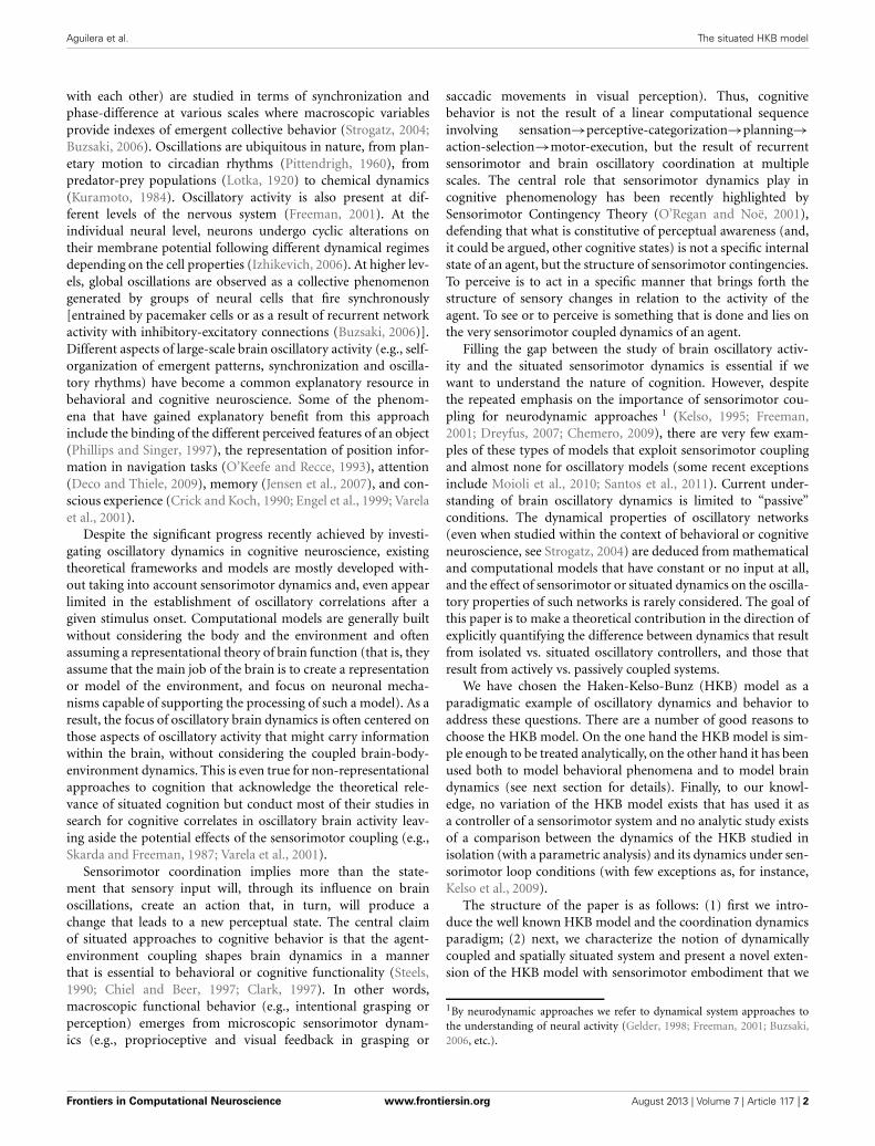
The relative phase or phase difference, ϕ, represents the orderparameter or collective variable that emerges from lower-levelinteractions of the two coupled oscillators, a and b are the cou-pling coefficients between the two oscillators, and �ω is thedifference between their intrinsic frequencies. Despite its sim-plicity, this equation captures a wide range of self-organizedphenomena. Different combinations of the control parameters a,b (or rather b/a) and �ω give rise to different collective behav-iors. For example, when shifting the value of �ω while the valuesof a and b are held fixed, the system experiences phase transitionsbetween three different modes of behavior: monostable, bistableand metastable (Figure 1).

The HKB has been used to model different kinds of coordina-tion phenomena but rarely used as a controller of an embodiedagent. To be fair to the HKB model, that was never the intentof the original authors. The HKB model (and its extended ver-sion) was rather conceived to describe the behavioral dynamics atthe macroscopic level (i.e., ϕ representing the collective variableof phase difference between two “behaving” oscillatory compo-nents, like fingers, oscillating armchairs in social coordination,etc.). It can be said that the HKB model was meant to capturethe global agent-environment dynamics, not any explicit behav-ior generating mechanism that is coupled through sensors andmotors to an environment. In addition, the HKB has also beenused to model inter-areal coordination in the cortex (Tognoliand Kelso, 2009), ignoring the potential influence of the cou-pling between brain and environment. In sum, previous uses of

0 1.57 3.14 4.71−1

0

1

2

3

4

−2

0

2

4

6

FIGURE 1 | Phase space of the extended HKB equation for fixed values

of the coupling coefficients a and b. The system exhibits three differentkinds of phase space depending on the control parameter �ω, showingmultistable (black), monostable (dark gray) or metastable (light gray)dynamics. The filled and empty dots represent respectively the attractorsand repellers of the system for different values of �ω. In this paper, theparameters used are choosen to ensure that the monostable region is theonly one that is stable for the agent.

Frontiers in Computational Neuroscience www.frontiersin.org August 2013 | Volume 7 | Article 117 | 3

Aguilera et al. The situated HKB model

the HKB model involve either full behavioral phenomena or “iso-lated” brain dynamics. However, there is a theoretical modelinggap that remains under-explored: the HKB as a controller of anagent that could modulate the control parameter (influenced bysensory input) through the behavior it generates when embod-ied in a robot. By filling in this gap we can address the followingquestions: How does the HKB model change its properties whensituated (i.e., under closed-loop sensorimotor coupling in a spa-cial environment)? Is there any qualitative change that comes outof this coupling? Can the behavioral properties of an oscillatory“brain”, or controller, be deduced from the study of the brain inisolation or under constant input? Or even from variation of theinput corresponding to those found in the coupled system? In thenext section, we will try to provide answers to these questionsby modeling a “situated HKB” and analytically solving the cou-pled agent-environment system and comparing it with isolatedand passively coupled conditions.

3. SITUATED HKB MODEL3.1. SENSORIMOTOR EMBODIMENT OF THE HKB EQUATIONIn this section we describe what we have called the situated HKBsystem: a robotic model where the HKB equation describes the“neural system” of the agent which is embodied with sensors andmotors and, in turn, situated in an environment. The agent hascircular body of radius R with two diametrically opposed motors(see Figure 2A), that can move forward or backwards with dif-ferent velocities in a 2D arena, and it has only one sensor thatprovides an input to the HKB neural controller.

Thereby, the HKB equation provides the macroscopic descrip-tion of the dynamics of the two coupled oscillators. It allows usto describe the behavior of the situated HKB system in the fol-lowing manner: (1) the agent has a “brain” where two regions(e.g., sensory and motor cortex) oscillate with their correspond-ing natural or intrinsic frequency (the difference between thesefrequencies is expressed by �ω0); (2) when a sensory input Imodifies the natural frequency of one of the oscillators (e.g., sen-sory cortex), the frequency difference term changes;3 (3) since thefrequency difference term is the control parameter of the phasedifference, ϕ, we can consider that the situated HKB agent mod-ulates its control parameter through sensorimotor contingencies:i.e., through the sensory changes that result from motor actionsand the displacements they generate.The dynamics of our agent is driven by:

ϕ = (�ω0 + I) − a · sin(ϕ) − 2b · sin(2ϕ) (2)

It is assumed that the agent is situated in a two-dimensionalenvironment where a radial gradient of a stimulus η is presentwith its peak on the origin of coordinates (one can interpret thisenvironment in different manners, e.g., as a light source or achemical gradient that diffuses from its center symmetrically inall directions).

3The term �ω of the original extended HKB equation has been substitutedby the term �ω0 + I, where I is the sensory input term whose effect is mathe-matically equivalent to changing the natural frequency of one of the oscillators(see Figure 2A).

A

C

B

FIGURE 2 | Situated HKB agent. (A) Structure of the agent, consisting in asensor, two oscillatory controllers, and two motors. (B) Sensorimotor loopof the agent. (C) Representation of the agent interacting with itsenvironment. The position and orientation of the agent respect to thecenter of the gradient are represented through the variables d and α.

With regard to the “sensory system” of the model, since theagent lives in a world of gradients, we designed its sensor not toperceive the absolute amount of stimulus present in the environ-ment but its change. Thus, the agent is sensitive to changes inη mediated by a sensitivity factor s that characterizes the sensorgain:

I = η · s

With respect to the “motor system” of the model, we define theactivations of the motors as functions of the state of the controller,

Mr(ϕ) = m · cos(ϕ)

Ml(ϕ) = m · cos(ϕ + c)

where Mr and Ml represent the right and left motors, respectively,m is a speed parameter, and c is a bias parameter that breaks thesymmetry between the right and left motors.

In this way, the brain-body-environment coupling can beunderstood as a process that repeats a cycled-course of fourstages involving successive transformations of I(t), �ω(t), ϕ(t),M(ϕ(t)) and back to I(t) (see Figure 2B). To fully describe themovement of the agent (see Appendix 6 for a complete deriva-tion of the agent’s description) we include an additional variabledescribing the angle α of the agent’s orientation relative to thepeak of the gradient (see Figure 2C).

Frontiers in Computational Neuroscience www.frontiersin.org August 2013 | Volume 7 | Article 117 | 4

Aguilera et al. The situated HKB model

In Appendix A, the reader can find detailed information onthe mathematical assumptions that we have considered for sim-plicity. As a direct result of assuming radial symmetry in theproblem: (1) we can use a polar coordinates system (distance dof the agent to the center of the gradient, and angle α of ori-entation of the agent relative to the peak of the gradient) as thereference frame, and (2) it is considered that the variation of thegradient in terms of polar coordinates does not depend on theangle, η(d,α) = η(d).

The process can be characterized as follows : (1) with themovement of the agent in the environment (variation of d) thesensor receives a new input I, (2) the input influences the firingrate of the oscillators, changing the frequency difference betweenthe HKB nodes (variation of �ω); (3) these frequency differ-ence translates to a change in the phase difference between theoscillators (variation of ϕ) and, finally, (4) the new value of thephase difference changes the state of the motors [variation ofM(ϕ)] moving the robot (variation of α) and starting the cycleagain.

In terms of polar coordinates and substituting values (seeAppendix A), the behavior of the agent {ϕ(t), M(ϕ(t))} can berepresented by a reduced set of equations describing the system-environment coupling:

ϕ = 1 + η · s − a · sin(ϕ) − 2b · sin(2ϕ)

η = cos(α) · (cos(ϕ) + cos(ϕ + c))

α = −sin(α)/η · (cos(ϕ) + cos(ϕ + c)) + (cos(ϕ)

−cos(ϕ + c)) (3)

where a, b, c, and s are the parameters of the system.

3.1.1. Behaviorial analysisWe have chosen a basic a gradient climbing4 task for our agent tosolve. That is, we ask the agent to climb up a linear gradient andmaintain itself as close as possible to the maximum peak. A simpletrial-and-error hand-tuning of the parameters gives us combi-nations that perform the desired behavior. We chose to adjustthe parameters to a = 5, b = 1, and c = 5, leaving unspecifiedthe sensitivity parameter s in order to have one free parameterto explore different kinds of behavior. This selection is arbi-trary (except for the relation of a/b, which was chosen to ensurethat the HKB is always in a monostable mode of functioning)but other combinations of parameters which result in gradient

4Gradient climbing is a minimal (yet not totally trivial) task, which iswidespread in nature. Most of small scale adaptive behavior occurs alongchemical gradients. The microscopic world is a world of gradients (like ther-mal gradients or light gradients but mostly chemical gradients). The adaptivebehavior of small animals (e.g., C. elegans) and individual motile cells (e.g.,bacteria but also animal cells migrating during development) is mostly agradient-related adaptive behavior. Navigating smell or heat gradients is alsoa stereotypical adaptive task for higher animals. Moreover many instances ofhigher-level behavior can also be interpreted as abstract gradient climbing(e.g., a human can move up a gradient of social popularity or economic wealththat might involve complex strategic decisions combined with an emotionalor sensitive gradient climbing of the perceived result of such strategies).

climbing behavior lead us to similar results in the analysis. Forthe experiments, the value of s will be defined in an intervalof [0, 15].

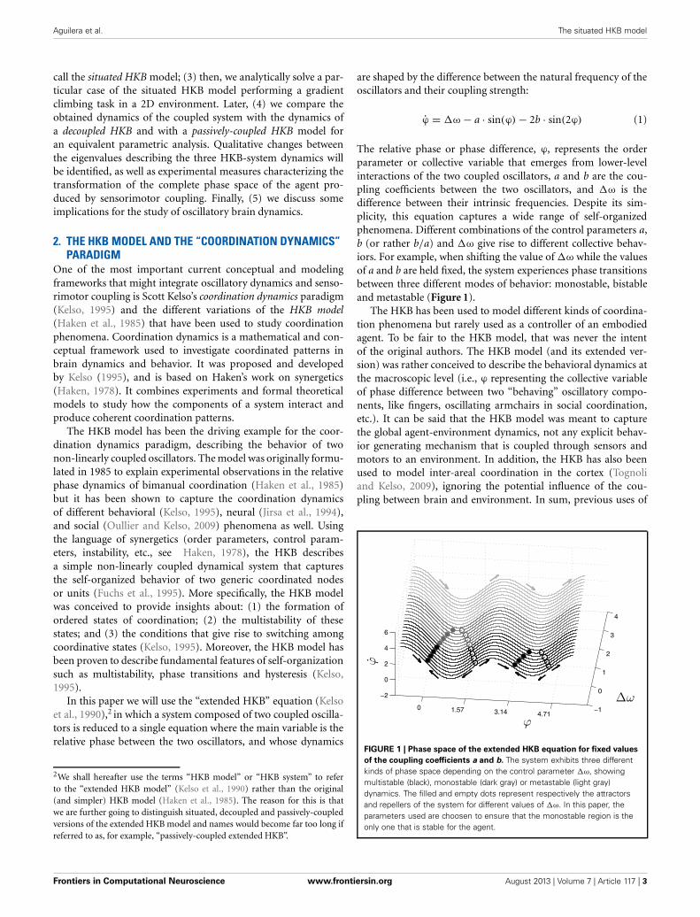
For these parameters, we see that the agent displays differ-ent behavioral strategies depending on the value of its sensitivityparameter s, ranging from: (1) for values of s ∈ [0, 2.4] display-ing cycloidal strategies where the agent turns over itself with acorkscrew-like movement, to (2) spiral paths where the agentslowly climbs the gradient, when s ∈ [2.6, 15]. At the frontierbetween these two behavioral strategies, we find (3) a criticalregion (s = 2.5) where the agent displays the most efficient gradi-ent navigation (in terms of time and trajectory efficiency), takinga curved approximation path ending in an spiral-circular patternaround the peak of the gradient. These different behaviors areshown in Figure 3, where the efficiency of each gradient climb-

ing strategy is computed with a parameter Fd = 1 − d(t = t1)d(t = 0)

, thatrepresents how close the agent gets to the center of the gradient ina given time (it is taken t1 = 40 s).

How do these behavioral strategies work? In the critical region(s = 2.5) the agent maps the highest gradient “sensation” withhigh activation of both motors, moving effectively toward thepeak of the gradient. As we increase the value of s, sensory stim-ulation is more intense, so the agent needs an strategy where theapproaching to the gradient peak is slower in order to maintain acompensated activation between the motors. On the other hand,when the value of s is decreased, the agent experiences difficultiesto maintain an equilibrated velocity for both motors, having toturn around periodically to find again a trajectory where a highsensor input is perceived.

3.2. ANALYTICAL SOLUTION FOR THE SITUATED-HKB SYSTEMWe shall now analytically solve the coupled brain-body-environment system in order to understand the emergence of thequalitatively different kinds of behavior that appear as we increasethe sensitivity s of the agent. As usual, if we want to understandthe behavior of an artifact modeled by a dynamical system, we willneed to calculate the linearization of the system around its fixedpoints (Strogatz, 2001).

Thus, if we take the situated-HKB system of equations to besolved,

ϕ = (1 + η(d,α) · s) − a sin(ϕ) − 2b · sin(2ϕ))

η = cos(α) · (cos(ϕ) + cos(ϕ + c))

α = −sin(α)/η · (cos(ϕ) + cos(ϕ + c)) + (cos(ϕ)

−cos(ϕ + c)) (4)

where the parameter s (sensitivity) will be used as a con-trol parameter to analyse the solutions in our range of inter-est s ∈ [0, 15], it is easy to find that two fixed points can beobtained: (1) the first one is an attractor with values of ϕ, η,α

at (0.11, 2.28,−π/2) and (2) the second one is a repeller at(2.53, 0.43,π/2).

Computing the Jacobian matrix of the system at the fixedpoints, and making an eigenvectors/eigenvalues analysis, we getthe behavior of our dynamical system around the regions ofits state space that bear qualitative significance. In Figure 4, it

Frontiers in Computational Neuroscience www.frontiersin.org August 2013 | Volume 7 | Article 117 | 5

Aguilera et al. The situated HKB model

FIGURE 3 | Different behaviors performed by the situated HKB system.

We observe how different gradient climbing strategies arise depending onthe value of s. For s = 1.5, the agent follows a cycloidal trajectory

continuously turning over itself, for s = 2.5 the agent finds a direct pathtoward the peak of the gradient, and for s = 8 the agent slowly approachesthe gradient peak following an spiral path.

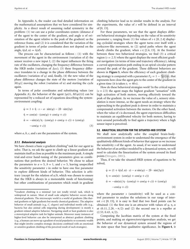
FIGURE 4 | Eigenvalues (λ1, λ2, and λ3) of the attractor (left) and

repeller (right) fixed points of the situated-HKB: force of the

attraction/repulsion vs. variation of the control parameter s. Real part(solid), Imaginary part (dashed).

is illustrated the range of different values of the eigenvalues(denoted by λ1,λ2, and λ3) at each of the fixed points, depend-ing on the parameter s (that corresponds to different observedbehavioral patterns for gradient climbing, see Figure 3). We findregions that present simple attractor/repulsion dynamics (whenλ1, λ2, λ3 are real numbers) whereas other regions present spiralattractions/repulsions (when λ1, λ2, λ3 have complex values).

In the following (see Figure 4), we show a detailed descrip-tion of the relations between eigenvalues and behavior, analyzingthe transitions of the eigenvalues in both the attractor and therepeller and focusing on the correspondences between those

transitions and the respective transitions in the behavioral modes(Figure 5). Concretely, we analyse the transitions from real tocomplex eigenvalues (from regular attraction to spiral attraction),and behavioral transitions from underdamped to overdampedbehavior (the system finds equilibrium with or without oscillat-ing) on one hand and from spiral to cycloidal movement of theagent on the other.

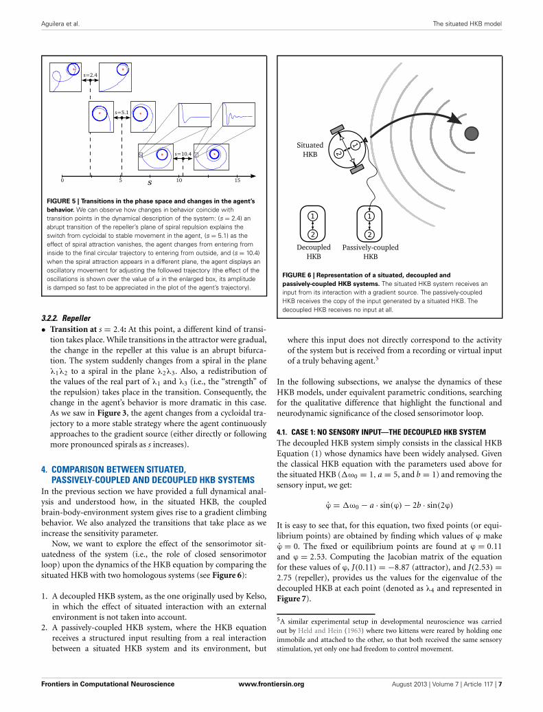
3.2.1. Attractor• Transition at s = 5.1: At this point, the attractor experiences a

change in its dynamics. An spiral attraction in the plane λ1λ2

disappears and the attraction of the system has no longer aspiral shape. At the same point, the approaching strategy ofthe agent experiences a change. For s < 5.1 the agent entersthe final stable circular trajectory from within, whereas for s >

5.1 the agent enters from outside the circle. This approachingstrategies correspond to a under-damped and a over-dampedbehavior of the {ϕ, η,α}−system, respectively.

• Transition at s = 10.4: The attractor changes again into a spi-ral shape, now in the plane λ2λ3. The behavioral change hereis more subtle. It appears at the initial turning behavior of theagent until it finds an stable trajectory and enters into the spiraltrajectory of the robot. When s < 10.4, the robot enters intothe trajectory by softly adjusting the value of α with an over-damped behavior, while when s > 10.4 the value of α oscillatesaround the trajectory, adjusting to the optimal value with anunder-damped behavior. This damping behavior also affectsϕ and η. Oscillations are too small to be clearly appreciatedin the trajectory of the robot. That is why in Figure 5, in theenlarged boxes, we just represent the orientation of the agentα, which shows how the robot adjusts its behavior to the finaltrajectory.

Frontiers in Computational Neuroscience www.frontiersin.org August 2013 | Volume 7 | Article 117 | 6

Aguilera et al. The situated HKB model

FIGURE 5 | Transitions in the phase space and changes in the agent’s

behavior. We can observe how changes in behavior coincide withtransition points in the dynamical description of the system: (s = 2.4) anabrupt transition of the repeller’s plane of spiral repulsion explains theswitch from cycloidal to stable movement in the agent, (s = 5.1) as theeffect of spiral attraction vanishes, the agent changes from entering frominside to the final circular trajectory to entering from outside, and (s = 10.4)when the spiral attraction appears in a different plane, the agent displays anoscillatory movement for adjusting the followed trajectory (the effect of theoscillations is shown over the value of α in the enlarged box, its amplitudeis damped so fast to be appreciated in the plot of the agent’s trajectory).

3.2.2. Repeller• Transition at s = 2.4: At this point, a different kind of transi-

tion takes place. While transitions in the attractor were gradual,the change in the repeller at this value is an abrupt bifurca-tion. The system suddenly changes from a spiral in the planeλ1λ2 to a spiral in the plane λ2λ3. Also, a redistribution ofthe values of the real part of λ1 and λ3 (i.e., the “strength” ofthe repulsion) takes place in the transition. Consequently, thechange in the agent’s behavior is more dramatic in this case.As we saw in Figure 3, the agent changes from a cycloidal tra-jectory to a more stable strategy where the agent continuouslyapproaches to the gradient source (either directly or followingmore pronounced spirals as s increases).

4. COMPARISON BETWEEN SITUATED,PASSIVELY-COUPLED AND DECOUPLED HKB SYSTEMS

In the previous section we have provided a full dynamical anal-ysis and understood how, in the situated HKB, the coupledbrain-body-environment system gives rise to a gradient climbingbehavior. We also analyzed the transitions that take place as weincrease the sensitivity parameter.

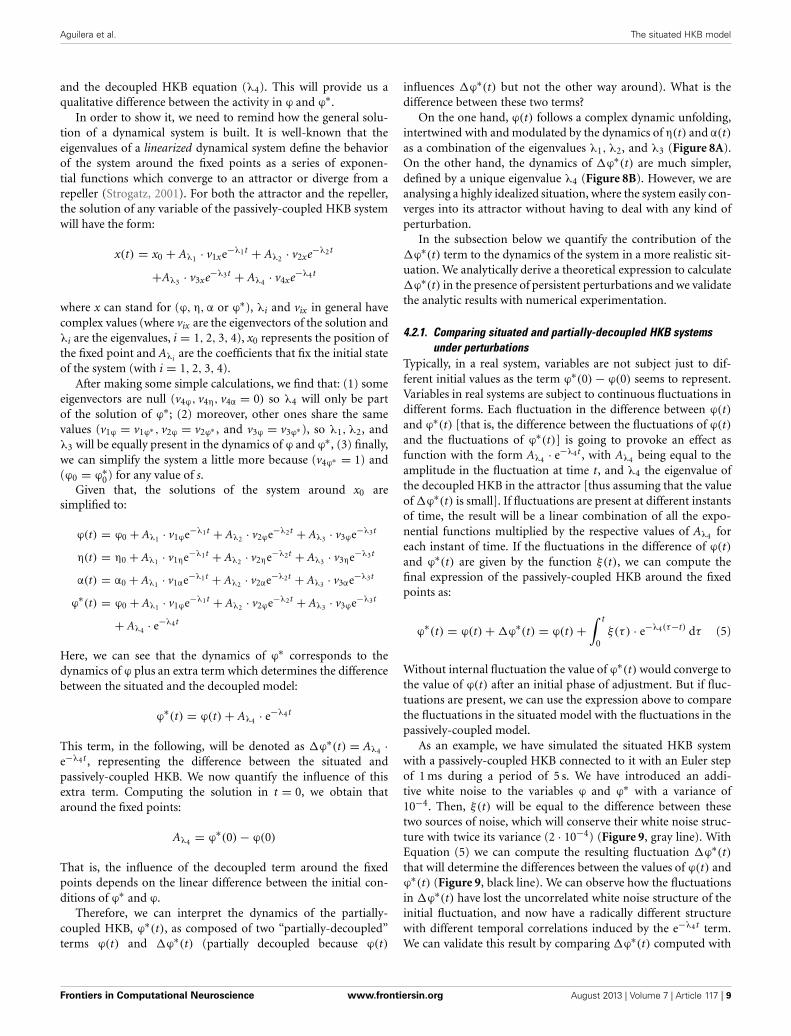
Now, we want to explore the effect of the sensorimotor sit-uatedness of the system (i.e., the role of closed sensorimotorloop) upon the dynamics of the HKB equation by comparing thesituated HKB with two homologous systems (see Figure 6):

1. A decoupled HKB system, as the one originally used by Kelso,in which the effect of situated interaction with an externalenvironment is not taken into account.

2. A passively-coupled HKB system, where the HKB equationreceives a structured input resulting from a real interactionbetween a situated HKB system and its environment, but

FIGURE 6 | Representation of a situated, decoupled and

passively-coupled HKB systems. The situated HKB system receives aninput from its interaction with a gradient source. The passively-coupledHKB receives the copy of the input generated by a situated HKB. Thedecoupled HKB receives no input at all.

where this input does not directly correspond to the activityof the system but is received from a recording or virtual inputof a truly behaving agent.5

In the following subsections, we analyse the dynamics of theseHKB models, under equivalent parametric conditions, searchingfor the qualitative difference that highlight the functional andneurodynamic significance of the closed sensorimotor loop.

4.1. CASE 1: NO SENSORY INPUT—THE DECOUPLED HKB SYSTEMThe decoupled HKB system simply consists in the classical HKBEquation (1) whose dynamics have been widely analysed. Giventhe classical HKB equation with the parameters used above forthe situated HKB (�ω0 = 1, a = 5, and b = 1) and removing thesensory input, we get:

ϕ = �ω0 − a · sin(ϕ) − 2b · sin(2ϕ)

It is easy to see that, for this equation, two fixed points (or equi-librium points) are obtained by finding which values of ϕ makeϕ = 0. The fixed or equilibrium points are found at ϕ = 0.11and ϕ = 2.53. Computing the Jacobian matrix of the equationfor these values of ϕ, J(0.11) = −8.87 (attractor), and J(2.53) =2.75 (repeller), provides us the values for the eigenvalue of thedecoupled HKB at each point (denoted as λ4 and represented inFigure 7).

5A similar experimental setup in developmental neuroscience was carriedout by Held and Hein (1963) where two kittens were reared by holding oneimmobile and attached to the other, so that both received the same sensorystimulation, yet only one had freedom to control movement.

Frontiers in Computational Neuroscience www.frontiersin.org August 2013 | Volume 7 | Article 117 | 7

Aguilera et al. The situated HKB model

FIGURE 7 | Eigenvalues for the decoupled HKB (λ4): Force of the

attraction/repulsion vs. variation of the control parameter s. Real part(solid), Imaginary part (dashed).

As we see, the eigenvalue is a real number at each fixed point,generating a simple pattern of attraction/repulsion in the dynam-ics of the system. Thus, the decoupled HKB alone cannot explainthe behavioral changes shown in Figure 4, where simple patternsof attraction/repulsion were transformed into spiral cycles, orabrupt changes arise changing the plane of the resulting patterns.The decoupled HKB system displays simple attraction and repul-sion forces around every fixed point and, therefore, the dynamicsof the system are going to be described by constant attraction andrepulsion forces regardless of the value of the parameter s.

In the situated HKB, we observed how the system displays“qualitatively different” behaviors, that is, behaviors that are notjust due to gradual variations of a single dynamical regime butas a consequence of a phase transition in the system dynamics.This is a phenomenon that also appears for the original HKBequation (under some conditions the system is able to switchfrom one attractor to another, see Kelso, 1995). However, thesituated-HKB with the parametric configuration used here (a = 5and b = 1) ϕ remains within the monostable region (except forbrief instants of time where the system visits the metastable regionbefore stabilizing in the monostable). Thus, it cannot display thephase transitions observed in the bistable configuration of theHKB. Taking the decoupled HKB as a reference, the situated HKBshould not present, in principle, qualitative changes that are notdue to external factors.

Thus, the observed phase transition in the situated HKB sys-tem cannot be explained by the dynamics of the HKB modelalone. Instead, the reason of this transition lies in the jointdynamics of the agent-environment system, as we illustratedwhen we solved the eigenvalues of the system. However, it is truethat, in a certain sense, the difference of dimensionality of thetwo models is enough to substantially modify the dynamics of thesystem, independently of the fact that these extra dimensions cor-respond to the agent or the environment. The very fact that thesituated HKB has three dimensions instead of one makes bothsystems are somewhat incommensurable.

The eigenvalues that determine the qualitative evolution of thesystem cannot be translated or mapped from the situated to thedecoupled conditions: the whole brain-body-environment systemdefines a new eigenvalue coordinate system where the “brain”contribution cannot be isolated. The main issue is that we aretalking about different systems: one consists of a single differen-tial equation and the other of three coupled differential equations.It is hard if not impossible to compare the dynamics of a onedimensional system with the dynamics of a three dimensionalsystem.

A B

FIGURE 8 | Comparison of the evolution of the system around the

attractor for (A) the situated HKB with s = 2.5 and (B) the decoupled

HKB (with �ω = 1, both with a = 5 and b = 1). The black line in thevertical axis represents the evolution over time (right vertical axis) of ϕ,which has been simulated during 6.5 s with an Euler step of 0.1 witharbitrary initial values of ϕ = 0.65,η = −2.78, and α = −2.07. The blue linerepresents the phase space of the HKB, representing the attractors as filleddots and the repellers as empty dots. We observe how the decoupled HKBis only affected by a simple attraction force with constant strength, while amuch richer dynamics is shown in the situated HKB, where different forcesof attraction interact to modulate the systems evolution.

The decoupled HKB is affected by a constant force of attrac-tion/repulsion (see Figure 8A) while the situated HKB is sub-ject to forces in three different dimensions that continuouslymodulate each other (Figure 8B). Note that even if we wereinducing a constant input (anywhere in the input range displayedby the situated system) the result will be equivalent. The next logi-cal step is to question whether the crucial factor when comparingthe HKB and the situated HKB systems is the specific structureof the input. In order to address this question we introduce thepassively-coupled HKB model where the HKB equation receivesthe exact same input as the freely behaving situated HKB, butwhose output has no effect.

4.2. CASE 2: EXTERNALLY STRUCTURED SENSORY INPUT—THEPASSIVELY-COUPLED HKB SYSTEM

We can model the passively-coupled HKB system by just adding anew variable ϕ∗ that receives the same input as ϕ [i.e., a new equa-tion ϕ∗ = 1 + η · s − a · sin(ϕ∗) − 2b · sin(2ϕ∗) is held togetherwith the previous system (see Equation 4)]. As a result, we have tosolve a four-dimensional system under the same conditions thanbefore (parameters a = 5, b = 1, and c = 5, and the value of sdefined in [0, 15]).

Analogously to the previous system we get two fixedpoints, an attractor at (0.11, 2.28, −π/2, 0.11) and a repeller at(2.53, 0.43,π/2, 2.53), and through the diagonalization of therespective jacobian matrices, four eigenvalues (λ1,λ2,λ3,λ4) areobtained.

As we will see below, although the term λ4 is decoupled fromthe activity of the situated HKB (and therefore independent of thetype of coupling, i.e., independent of the value of s), the behaviorof the new variable ϕ∗ will necessarily be described by a combina-tion of the eigenvalues of the situated HKB system (λ1, λ2, λ3)

Frontiers in Computational Neuroscience www.frontiersin.org August 2013 | Volume 7 | Article 117 | 8

Aguilera et al. The situated HKB model

and the decoupled HKB equation (λ4). This will provide us aqualitative difference between the activity in ϕ and ϕ∗.

In order to show it, we need to remind how the general solu-tion of a dynamical system is built. It is well-known that theeigenvalues of a linearized dynamical system define the behaviorof the system around the fixed points as a series of exponen-tial functions which converge to an attractor or diverge from arepeller (Strogatz, 2001). For both the attractor and the repeller,the solution of any variable of the passively-coupled HKB systemwill have the form:

x(t) = x0 + Aλ1 · v1xe−λ1t + Aλ2 · v2xe−λ2t

+Aλ3 · v3xe−λ3t + Aλ4 · v4xe−λ4t

where x can stand for (ϕ, η,α or ϕ∗), λi and vix in general havecomplex values (where vix are the eigenvectors of the solution andλi are the eigenvalues, i = 1, 2, 3, 4), x0 represents the position ofthe fixed point and Aλi are the coefficients that fix the initial stateof the system (with i = 1, 2, 3, 4).

After making some simple calculations, we find that: (1) someeigenvectors are null (v4ϕ, v4η, v4α = 0) so λ4 will only be partof the solution of ϕ∗; (2) moreover, other ones share the samevalues (v1ϕ = v1ϕ∗ , v2ϕ = v2ϕ∗ , and v3ϕ = v3ϕ∗ ), so λ1,λ2, andλ3 will be equally present in the dynamics of ϕ and ϕ∗, (3) finally,we can simplify the system a little more because (v4ϕ∗ = 1) and(ϕ0 = ϕ∗

0) for any value of s.Given that, the solutions of the system around x0 are

simplified to:

ϕ(t) = ϕ0 + Aλ1 · v1ϕe−λ1t + Aλ2 · v2ϕe−λ2t + Aλ3 · v3ϕe−λ3t

η(t) = η0 + Aλ1 · v1ηe−λ1t + Aλ2 · v2ηe−λ2t + Aλ3 · v3ηe−λ3t

α(t) = α0 + Aλ1 · v1αe−λ1t + Aλ2 · v2αe−λ2t + Aλ3 · v3αe−λ3t

ϕ∗(t) = ϕ0 + Aλ1 · v1ϕe−λ1t + Aλ2 · v2ϕe−λ2t + Aλ3 · v3ϕe−λ3t

+ Aλ4 · e−λ4t

Here, we can see that the dynamics of ϕ∗ corresponds to thedynamics of ϕ plus an extra term which determines the differencebetween the situated and the decoupled model:

ϕ∗(t) = ϕ(t) + Aλ4 · e−λ4t

This term, in the following, will be denoted as �ϕ∗(t) = Aλ4 ·e−λ4t , representing the difference between the situated andpassively-coupled HKB. We now quantify the influence of thisextra term. Computing the solution in t = 0, we obtain thataround the fixed points:

Aλ4 = ϕ∗(0) − ϕ(0)

That is, the influence of the decoupled term around the fixedpoints depends on the linear difference between the initial con-ditions of ϕ∗ and ϕ.

Therefore, we can interpret the dynamics of the partially-coupled HKB, ϕ∗(t), as composed of two “partially-decoupled”terms ϕ(t) and �ϕ∗(t) (partially decoupled because ϕ(t)

influences �ϕ∗(t) but not the other way around). What is thedifference between these two terms?

On the one hand, ϕ(t) follows a complex dynamic unfolding,intertwined with and modulated by the dynamics of η(t) and α(t)as a combination of the eigenvalues λ1,λ2, and λ3 (Figure 8A).On the other hand, the dynamics of �ϕ∗(t) are much simpler,defined by a unique eigenvalue λ4 (Figure 8B). However, we areanalysing a highly idealized situation, where the system easily con-verges into its attractor without having to deal with any kind ofperturbation.

In the subsection below we quantify the contribution of the�ϕ∗(t) term to the dynamics of the system in a more realistic sit-uation. We analytically derive a theoretical expression to calculate�ϕ∗(t) in the presence of persistent perturbations and we validatethe analytic results with numerical experimentation.

4.2.1. Comparing situated and partially-decoupled HKB systemsunder perturbations

Typically, in a real system, variables are not subject just to dif-ferent initial values as the term ϕ∗(0) − ϕ(0) seems to represent.Variables in real systems are subject to continuous fluctuations indifferent forms. Each fluctuation in the difference between ϕ(t)and ϕ∗(t) [that is, the difference between the fluctuations of ϕ(t)and the fluctuations of ϕ∗(t)] is going to provoke an effect asfunction with the form Aλ4 · e−λ4t , with Aλ4 being equal to theamplitude in the fluctuation at time t, and λ4 the eigenvalue ofthe decoupled HKB in the attractor [thus assuming that the valueof �ϕ∗(t) is small]. If fluctuations are present at different instantsof time, the result will be a linear combination of all the expo-nential functions multiplied by the respective values of Aλ4 foreach instant of time. If the fluctuations in the difference of ϕ(t)and ϕ∗(t) are given by the function ξ(t), we can compute thefinal expression of the passively-coupled HKB around the fixedpoints as:

ϕ∗(t) = ϕ(t) + �ϕ∗(t) = ϕ(t) +∫ t

0ξ(τ) · e−λ4(τ−t) dτ (5)

Without internal fluctuation the value of ϕ∗(t) would converge tothe value of ϕ(t) after an initial phase of adjustment. But if fluc-tuations are present, we can use the expression above to comparethe fluctuations in the situated model with the fluctuations in thepassively-coupled model.

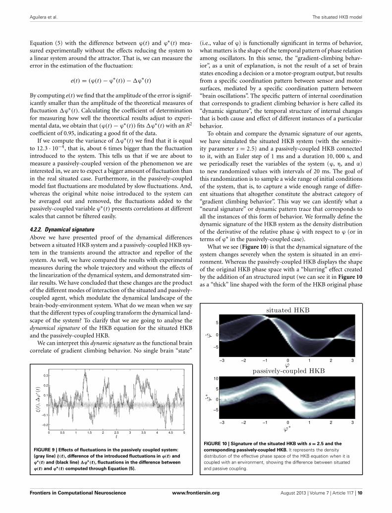
As an example, we have simulated the situated HKB systemwith a passively-coupled HKB connected to it with an Euler stepof 1 ms during a period of 5 s. We have introduced an addi-tive white noise to the variables ϕ and ϕ∗ with a variance of10−4. Then, ξ(t) will be equal to the difference between thesetwo sources of noise, which will conserve their white noise struc-ture with twice its variance (2 · 10−4) (Figure 9, gray line). WithEquation (5) we can compute the resulting fluctuation �ϕ∗(t)that will determine the differences between the values of ϕ(t) andϕ∗(t) (Figure 9, black line). We can observe how the fluctuationsin �ϕ∗(t) have lost the uncorrelated white noise structure of theinitial fluctuation, and now have a radically different structurewith different temporal correlations induced by the e−λ4t term.We can validate this result by comparing �ϕ∗(t) computed with

Frontiers in Computational Neuroscience www.frontiersin.org August 2013 | Volume 7 | Article 117 | 9

Aguilera et al. The situated HKB model

Equation (5) with the difference between ϕ(t) and ϕ∗(t) mea-sured experimentally without the effects reducing the system toa linear system around the attractor. That is, we can measure theerror in the estimation of the fluctuation:

e(t) = (ϕ(t) − ϕ∗(t)) − �ϕ∗(t)

By computing e(t) we find that the amplitude of the error is signif-icantly smaller than the amplitude of the theoretical measures offluctuation �ϕ∗(t). Calculating the coefficient of determinationfor measuring how well the theoretical results adjust to experi-mental data, we obtain that (ϕ(t) − ϕ∗(t)) fits �ϕ∗(t) with an R2

coefficient of 0.95, indicating a good fit of the data.If we compute the variance of �ϕ∗(t) we find that it is equal

to 12.3 · 10−4, that is, about 6 times bigger than the fluctuationintroduced to the system. This tells us that if we are about tomeasure a passively-coupled version of the phenomenon we areinterested in, we are to expect a bigger amount of fluctuation thanin the real situated case. Furthermore, in the passively-coupledmodel fast fluctuations are modulated by slow fluctuations. And,whereas the original white noise introduced to the system canbe averaged out and removed, the fluctuations added to thepassively-coupled variable ϕ∗(t) presents correlations at differentscales that cannot be filtered easily.

4.2.2. Dynamical signatureAbove we have presented proof of the dynamical differencesbetween a situated HKB system and a passively-coupled HKB sys-tem in the transients around the attractor and repellor of thesystem. As well, we have compared the results with experimentalmeasures during the whole trajectory and without the effects ofthe linearization of the dynamical system, and demonstrated sim-ilar results. We have concluded that these changes are the productof the different modes of interaction of the situated and passively-coupled agent, which modulate the dynamical landscape of thebrain-body-environment system. What do we mean when we saythat the different types of coupling transform the dynamical land-scape of the system? To clarify that we are going to analyse thedynamical signature of the HKB equation for the situated HKBand the passively-coupled HKB.

We can interpret this dynamic signature as the functional braincorrelate of gradient climbing behavior. No single brain “state”

FIGURE 9 | Effects of fluctuations in the passively coupled system:

(gray line) ξ(t), difference of the introduced fluctuations in ϕ(t) and

ϕ∗(t) and (black line) �ϕ∗(t), fluctuations in the difference between

ϕ(t) and ϕ∗(t) computed through Equation (5).

(i.e., value of ϕ) is functionally significant in terms of behavior,what matters is the shape of the temporal pattern of phase relationamong oscillators. In this sense, the “gradient-climbing behav-ior”, as a unit of explanation, is not the result of a set of brainstates encoding a decision or a motor-program output, but resultsfrom a specific coordination pattern between sensor and motorsurfaces, mediated by a specific coordination pattern between“brain oscillations”. The specific pattern of internal coordinationthat corresponds to gradient climbing behavior is here called its“dynamic signature”, the temporal structure of internal changesthat is both cause and effect of different instances of a particularbehavior.

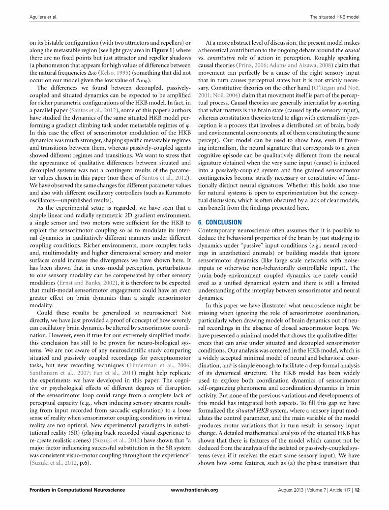
To obtain and compare the dynamic signature of our agents,we have simulated the situated HKB system (with the sensitiv-ity parameter s = 2.5) and a passively-coupled HKB connectedto it, with an Euler step of 1 ms and a duration 10, 000 s, andwe periodically reset the variables of the system (ϕ, η, and α)to new randomized values with intervals of 20 ms. The goal ofthis randomization is to sample a wide range of initial conditionsof the system, that is, to capture a wide enough range of differ-ent situations that altogether constitute the abstract category of“gradient climbing behavior”. This way we can identify what a“neural signature” or dynamic pattern trace that corresponds toall the instances of this form of behavior. We formally define thedynamic signature of the HKB system as the density distributionof the derivative of the relative phase ϕ with respect to ϕ (or interms of ϕ∗ in the passively-coupled case).

What we see (Figure 10) is that the dynamical signature of thesystem changes severely when the system is situated in an envi-ronment. Whereas the passively-coupled HKB displays the shapeof the original HKB phase space with a “blurring” effect createdby the addition of an structured input (we can see it in Figure 10as a “thick” line shaped with the form of the HKB original phase

FIGURE 10 | Signature of the situated HKB with s = 2.5 and the

corresponding passively-coupled HKB. It represents the densitydistribution of the effective phase space of the HKB equation when it iscoupled with an environment, showing the difference between situatedand passive coupling.

Frontiers in Computational Neuroscience www.frontiersin.org August 2013 | Volume 7 | Article 117 | 10

Aguilera et al. The situated HKB model

space), in the situated system the structure of the dynamical sig-nature no longer resembles the original HKB phase space. Thesituated system has modulated or re-shaped its state space into aspecific pattern through sensorimotor coordination.

5. RECAPITULATION, DISCUSSION, AND INTERPRETATIONOF RESULTS

We have just shown how the HKB system displays qualitativelydifferent dynamics under situated conditions, as compared todecoupled and passively-coupled conditions. We can recapitulatethe main results as follows:

1. Transitions between qualitatively different types of sensori-motor behavior, that are generated by the situated HKB withincreasing sensitivity, cannot be deduced from the behaviorof the decoupled HKB nor from the analysis of the passivelycoupled HKB alone. The nature of these transitions can onlybe revealed through the analysis of the whole brain-body-environment system.

2. Even for a single fixed value of the sensitivity parameter thetransient trajectory of the situated HKB system toward itsattractor is far from trivial, it unfolds in different ways at differ-ent temporal scales. The transient trajectory of the decoupledHKB system, instead, is relatively simple and monotonic.

3. A passively-coupled agent receiving an input generated by asituated agent shows correlated and amplified fluctuations thatare not present in the situated agent.

4. Finally, the dynamical signature of the agents shows us how thetype of coupling (passive or situated) severely transforms thephase space of the HKB system. The specificity of functionalneural signatures is lost when studying the brain out of theclosed sensorimotor loop, even if it is subjected to exactly thesame input.

These kinds of differences between situated and decoupled oscil-latory controllers illustrate how much we would miss if weanalysed the “brain” of an agent isolated from its embodied sit-uatedness in an environment. On the one hand, the brain-body-environment system constitutes a dynamical holistic continuumwhere phase transitions can take place, without necessarily cor-responding to phase transitions that would occur in an isolatedbrain. Quite the opposite, in general this joint dynamical struc-ture would be hardly deduced from the isolated controller of anagent. On the other hand, the unfolding of behavior shown by asystem is modulated by the continuous interplay with the envi-ronment at different time-scales that generally are not present inthe dynamics of the controller system alone, giving rise to muchricher behavioral dynamics.

Our situated HKB is a case of double coordination: senso-rimotor coordination of the coordinated dynamics of the twooscillatory components (modeled by the HKB equation). What iscrucial is the fact that under situated conditions the dynamics of theHKB can be modulated by the precise and interactively structuredcoordination between its internal dynamics and the sensorimo-tor environment. The mode in which sensory input (the controlparameter) changes as a function of the motor output (which is inturn generated by internal dynamics) through the environment,

makes possible this higher order coordination. It can be said thatthe agent modulates its internal dynamics through sensorimotorcoordination, in a manner that is not available to the decou-pled or passively-coupled system, resulting in functionally specificinternal patterns that we have demonstrated with the dynamicsignature.

We can learn about the HKB system as a model in(sensori)motor control and oscillatory brain dynamics.Notwithstanding are the important contributions that thismodel has brought with its application to behavioral and neuralsciences. There are, however, important limitations on the type ofmodeling. The most relevant for us is that, for the paradigmaticcases (like finger coordination), there is no genuine sensorimotorcoupling being modeled. A subject is asked to move the fingers incoordination with a metronome but this is the only coupling thatexists. Finger movement is a motor task, driven by a sensory cue(the pace of the metronome) but it is not a sensorimotor task. It isunnatural to instruct or constrain habitual behavior in responseto the tight instructions of an experimenter. Human and animalbehavior is generally the result of a “free” sensorimotor couplingwhere every motor variation carries with it a sensory variation,bringing about a coordinated behavioral pattern. In terms ofthe finger coordination experimental paradigm, the “naturalsituation” would resemble one where a finger movement altersthe metronome’s pace, which in turn alters the finger movement,etc. The HKB model has been applied to other, more complextasks (like social coordination) but, to our knowledge and despitethe emphasis of many advocates of sensorimotor dynamics(Kelso, 1995; Chemero, 2001, 2009), there is no available modelof HKB for sensorimotor coordination itself. It was thereforecrucial to understand the dynamics of the situated HKB toexplore in detail the way in which coordination dynamics canbe radically altered when oscillatory dynamics appear coupledto sensorimotor dynamics. The HKB equation has been usedto model cases of sensorimotor coupling such as (Kelso et al.,2009), where a human subject receives sensory feedback from acomputer screen, and the human’s behavior in turn affects thecomputer. The novelty of the situated HKB model is that thecoupling is spatial and the HKB is not meant to capture the globalfeedback dynamics, but is used directly as a robotic controller. Aswell, whereas in the experiment above part of the interaction wasan human subject, the situated HKB is a model which can be fullydescribed by just three equations. This is a great advantage interms of dynamical analysis, allowing us a much deeper analysisof the system’s behavior.

It is important to note that the present paper has focusedon the most simple configuration of the HKB model; with anextremely simplified body and environment. Regarding the inter-nal configuration of the HKB, we have studied it under thesimplest parametric configuration that produces a single attrac-tor instead of two or none, which is due to the a/b coefficientvalue that we kept fixed. Even for this simple configuration wehave found qualitative differences of the transient dynamics of thesystem before falling into the attractor—see ϕ = 0.11 and tran-sient dynamics around (−1, 2.50) in Figure 8. The behavior ofthe system shows strong differences under the situated and decou-pled conditions. But the HKB can display much richer behavior

Frontiers in Computational Neuroscience www.frontiersin.org August 2013 | Volume 7 | Article 117 | 11

Aguilera et al. The situated HKB model

on its bistable configuration (with two attractors and repellers) oralong the metastable region (see light gray area in Figure 1) wherethere are no fixed points but just attractor and repeller shadows(a phenomenon that appears for high values of difference betweenthe natural frequencies �ω (Kelso, 1995) (something that did notoccur on our model given the low value of �ω0).

The differences we found between decoupled, passively-coupled and situated dynamics can be expected to be amplifiedfor richer parametric configurations of the HKB model. In fact, ina parallel paper (Santos et al., 2012), some of this paper’s authorshave studied the dynamics of the same situated HKB model per-forming a gradient climbing task under metastable regimes of ϕ.In this case the effect of sensorimotor modulation of the HKBdynamics was much stronger, shaping specific metastable regimesand transitions between them, whereas passively-coupled agentsshowed different regimes and transitions. We want to stress thatthe appearance of qualitative differences between situated anddecoupled systems was not a contingent results of the parame-ter values chosen in this paper (nor those of Santos et al., 2012).We have observed the same changes for different parameter valuesand also with different oscillatory controllers (such as Kuramotooscillators—unpublished results).

As the experimental setup is regarded, we have seen that asimple linear and radially symmetric 2D gradient environment,a single sensor and two motors were sufficient for the HKB toexploit the sensorimotor coupling so as to modulate its inter-nal dynamics in qualitatively different manners under differentcoupling conditions. Richer environments, more complex tasksand, multimodality and higher dimensional sensory and motorsurfaces could increase the divergences we have shown here. Ithas been shown that in cross-modal perception, perturbationsto one sensory modality can be compensated by other sensorymodalities (Ernst and Banks, 2002), it is therefore to be expectedthat multi-modal sensorimotor engagement could have an evengreater effect on brain dynamics than a single sensorimotormodality.

Could these results be generalized to neuroscience? Notdirectly, we have just provided a proof of concept of how severelycan oscillatory brain dynamics be altered by sensorimotor coordi-nation. However, even if true for our extremely simplified modelthis conclusion has still to be proven for neuro-biological sys-tems. We are not aware of any neuroscientific study comparingsituated and passively coupled recordings for perceptuomotortasks, but new recording techniques (Linderman et al., 2006;Santhanam et al., 2007; Fan et al., 2011) might help replicatethe experiments we have developed in this paper. The cogni-tive or psychological effects of different degrees of disruptionof the sensorimotor loop could range from a complete lack ofperceptual capacity (e.g., when inducing sensory streams result-ing from input recorded from saccadic exploration) to a loosesense of reality when sensorimotor coupling conditions in virtualreality are not optimal. New experimental paradigms in substi-tutional reality (SR) (playing back recorded visual experience tore-create realistic scenes) (Suzuki et al., 2012) have shown that “amajor factor influencing successful substitution in the SR systemwas consistent visuo-motor coupling throughout the experience”(Suzuki et al., 2012, p.6).

At a more abstract level of discussion, the present model makesa theoretical contribution to the ongoing debate around the causalvs. constitutive role of action in perception. Roughly speakingcausal theories (Prinz, 2006; Adams and Aizawa, 2008) claim thatmovement can perfectly be a cause of the right sensory inputthat in turn causes perceptual states but it is not strictly neces-sary. Constitutive theories on the other hand (O’Regan and Noë,2001; Noë, 2004) claim that movement itself is part of the percep-tual process. Causal theories are generally internalist by assertingthat what matters is the brain state (caused by the sensory input),whereas constitution theories tend to align with externalism (per-ception is a process that involves a distributed set of brain, bodyand environmental components, all of them constituting the samepercept). Our model can be used to show how, even if favor-ing internalism, the neural signature that corresponds to a givencognitive episode can be qualitatively different from the neuralsignature obtained when the very same input (cause) is inducedinto a passively-coupled system and fine grained sensorimotorcontingencies become strictly necessary or constitutive of func-tionally distinct neural signatures. Whether this holds also truefor natural systems is open to experimentation but the concep-tual discussion, which is often obscured by a lack of clear models,can benefit from the findings presented here.

6. CONCLUSIONContemporary neuroscience often assumes that it is possible todeduce the behavioral properties of the brain by just studying itsdynamics under “passive” input conditions (e.g., neural record-ings in anesthetized animals) or building models that ignoresensorimotor dynamics (like large scale networks with noise-inputs or otherwise non-behaviorally controllable input). Thebrain-body-environment coupled dynamics are rarely consid-ered as a unified dynamical system and there is still a limitedunderstanding of the interplay between sensorimotor and neuraldynamics.

In this paper we have illustrated what neuroscience might bemissing when ignoring the role of sensorimotor coordination,particularly when drawing models of brain dynamics out of neu-ral recordings in the absence of closed sensorimotor loops. Wehave presented a minimal model that shows the qualitative differ-ences that can arise under situated and decoupled sensorimotorconditions. Our analysis was centered in the HKB model, which isa widely accepted minimal model of neural and behavioral coor-dination, and is simple enough to facilitate a deep formal analysisof its dynamical structure. The HKB model has been widelyused to explore both coordination dynamics of sensorimotorself-organizing phenomena and coordination dynamics in brainactivity. But none of the previous variations and developments ofthis model has integrated both aspects. To fill this gap we haveformalized the situated HKB system, where a sensory input mod-ulates the control parameter, and the main variable of the modelproduces motor variations that in turn result in sensory inputchange. A detailed mathematical analysis of the situated HKB hasshown that there is features of the model which cannot not bededuced from the analysis of the isolated or passively-coupled sys-tems (even if it receives the exact same sensory input). We haveshown how some features, such as (a) the phase transition that

Frontiers in Computational Neuroscience www.frontiersin.org August 2013 | Volume 7 | Article 117 | 12

Aguilera et al. The situated HKB model

takes place modifying a sensitivity parameter, (b) the attractionpatterns, (c) the neurodynamic signatures, and (d) the mod-ulatory capacity of the situated system. All of them need tobe explained by a framework that takes into account the cou-pled dynamics of the brain-body-environment system. How farthese results can be generalized to experimental neuroscienceremains open to experimentation, the present contribution wasa theoretical one aiming at making a formal characterizationand a proof of concept of how sensorimotor dynamics can alterthe oscillatory coordination properties of behavior-generatingmechanisms.

ACKNOWLEDGMENTSThe work presented here benefited from the economic supportof the Retecog Network (Red Española de Ciencia Cognitiva,FFI2010-09796-E, Ministerio de Ciencia e Innovación. AccionesComplementarias a Proyectos de Investigación Fundamental no

orientada, Government of Spain) that financed a 1 month stanceof Dr. Manuel Bedia, Miguel Aguilera and Bruno Santos atthe IAS-Research Centre for Life, Mind and Society at theUniversity of the Basque Country. Miguel Aguilera and ManuelG. Bedia were supported in part by the project TIN2011-24660funded by the Spanish “Ministerio de Ciencia e Innovación”.Miguel Aguilera currently holds a FPU predoctoral fellow-ship from the Spanish “Ministerio de Educación.” Bruno A.Santos acknowledges financial support from Brazilian NationalCouncil of Research, CNPq. During the development of thispaper Dr. Xabier E. Barandiaran hold a postdoctoral positionfunded by FP7 project eSMCs IST-270212. XEB also acknowl-edges funding from research project “Autonomía y Nivelesde Organización” financed by the Spanish Government (ref.FFI2011-25665) and IAS-Research group funding IT590-13 fromthe Basque Government (of which MB and MA are alsocollaborators).

REFERENCESAdams, F., and Aizawa, K. (2008). The

Bounds of Cognition. Malden, MA:John Wiley & Sons.

Ashby, W. R. (1952). Design for aBrain. 2nd Edn. New York, NY: JohnWiley.

Beer, R. D. (1990). Intelligenceas Adaptive Behaviour: AnExperiment in ComputationalNeuroethology. Boston: AcademicPress.

Beer, R. D. (1997). The dynamicsof adaptive behavior: a researchprogram. Rob. Auton. Syst. 20,257–289. doi: 10.1016/S0921-8890(96)00063-2

Brooks, R. A. (1991). Intelligence with-out representation. Artif. Intell. 47,139–159. doi: 10.1016/0004-3702(91)90053-M

Buzsaki, G. (2006). Rhythms ofthe Brain. 1st Edn. Oxford:Oxford University Press.doi: 10.1093/acprof:oso/9780195301069.001.0001

Carruthers, P. (2006). TheArchitecture of the Mind.Oxford: Oxford University Press.doi: 10.1093/acprof:oso/9780199207077.001.0001

Chemero, A. (2001). Dynamicalexplanation and mental repre-sentations. Trends Cogn. Sci. 5,141–142. doi: 10.1016/S1364-6613(00)01627-2

Chemero, A. (2009). Radical EmbodiedCognitive Science. Cambridge, MA:The MIT Press.

Chiel, H., and Beer, R. (1997). Thebrain has a body: adaptive behav-ior emerges from interactions ofnervous system, body and envi-ronment. Trends Neurosci. 20,553–557. doi: 10.1016/S0166-2236(97)01149-1

Clark, A. (1997). The dynamical chal-lenge. Cogn. Sci. 21, 461–481. doi:10.1207/s15516709cog2104_3

Crick, F., and Koch, C. (1990). Towardsa neurobiological theory of con-sciousness. Semi. Neurosci. 2,263–275.

Deco, G., and Thiele, A. (2009).Attention – oscillations and neu-ropharmacology. Eur. J. Neurosci.30, 347–354. doi: 10.1111/j.1460-9568.2009.06833.x

Dewey, J. (1896). The reflex arc con-cept in psychology. Psychol. Rev. 3,357–370. doi: 10.1037/h0070405

Dewey, J. (1922). Human Nature andConduct. New York, NY: CourierDover Publications.

Dreyfus, H. L. (2007). Why hei-deggerian AI failed and howfixing it would require makingit more heideggerian. Philos.Psychol. 20, 247–268. doi: 10.1080/09515080701239510

Engel, A. K., Fries, P., König, P., Brecht,M., and Singer, W. (1999). Temporalbinding, binocular rivalry, and con-sciousness. Conscious. Cogn. 8,128–151. doi: 10.1006/ccog.1999.0389

Ernst, M. O., and Banks, M. S. (2002).Humans integrate visual and hapticinformation in a statistically opti-mal fashion. Nature 415, 429–433.doi: 10.1038/415429a

Fan, D., Rich, D., Holtzman, T., Ruther,P., Dalley, J. W., Lopez, A., et al.(2011). A wireless multi-channelrecording system for freely behav-ing mice and rats. PLoS ONE6:e22033. doi: 10.1371/journal.pone.0022033

Fodor, J. A. (1983). The Modularityof Mind: An Essay on FacultyPsychology. Cambridge, MA: MITPress.

Freeman, W. J. (2001). How BrainsMake Up Their Minds. 1st Edn.New York, NY: Columbia UniversityPress.

Fuchs, A., Jirsa, V., Haken, H., andKelso, J. A. S. (1995). Extending theHKB model of coordinated move-ment to oscillators with differenteigenfrequencies. Biol. Cybern. 74,21–30. doi: 10.1007/BF00199134

Haken, H. (1978). Synergetics: Anintroduction: Nonequilibrium phasetransitions and self-organization inphysics, chemistry, and biology. 2ndEdn. Berlin: Springer-Verlag.

Haken, H., Kelso, J. A. S., and Bunz, H.(1985). A theoretical model of phasetransitions in human hand move-ments. Biol. Cybern. 51, 347–356.doi: 10.1007/BF00336922

Held, R., and Hein, A. (1963).Movement-produced stimula-tion in the development of visuallyguided behavior. J. Comp. Physiol.Psychol. 56, 872–876. doi: 10.1037/h0040546

Izhikevich, E. M. (2006). DynamicalSystems in Neuroscience: TheGeometry of Excitability andBursting. 1st Edn. Cambridge, MA:The MIT Press.

Jensen, O., Kaiser, J., and Lachaux, J.-P.(2007). Human gamma-frequencyoscillations associated with atten-tion and memory. Trends Neurosci.30, 317–324. doi: 10.1016/j.tins.2007.05.001

Jirsa, V. K., Friedrich, R., Haken, H.,and Kelso, J. A. S. (1994). A theo-retical model of phase transitions inthe human brain. Biol. Cybern. 71,27–35. doi: 10.1007/BF00198909

Kelso, J. A. S. (1995). Dynamic Patterns:The Self-organization of Brain andBehavior. Cambridge, MA: MITPress.

Kelso, J. A. S., de Guzman, G. C.,Reveley, C., and Tognoli, E. (2009).Virtual partner interaction (VPI):exploring novel behaviors viacoordination dynamics. PLoS ONE4:e5749. doi: 10.1371/journal.pone.0005749

Kelso, J. A. S., Delcolle, J., and Schöner,G. (1990). “Action-perception asa pattern formation process”, inAttention and Performance XIII,ed M. Jeannerod (Hillsdale, NJ:Erlbaum), 139–169.

Kuramoto, Y. (1984). ChemicalOscillations, Waves, and Turbulence.Berlin: Springer Verlag. doi:10.1007/978-3-642-69689-3

Linderman, M. D., Gilja, V.,Santhanam, G., Afshar, A., Ryu, S.,Meng, T. H., et al. (2006). Neuralrecording stability of chronic elec-trode arrays in freely behavingprimates. Conf. Proc. IEEE Eng.Med. Biol. Soc. 1, 4387–4391. doi:10.1109/IEMBS.2006.260814

Lotka, A. (1920). Analytical noteon certain rhythmic relations inorganic systems. Proc. Natl. Acad.Sci. U.S.A. 6:410. doi: 10.1073/pnas.6.7.410

Merleau-Ponty, M. (1942). TheStructure of Behavior. Boston:Beacon Press.

Moioli, R. C., Vargas, P. A., andHusbands, P. (2010). “Exploringthe Kuramoto model of coupledoscillators in minimally cognitiveevolutionary robotics tasks,” inIEEE Congress on EvolutionaryComputation (CEC) (Barcelona),2483–2490.

Noë, A. (2004). Action in Perception.Cambridge, MA: MIT Press.

O’Keefe, J., and Recce, M. (1993). Phaserelationship between hippocampalplace units and the EEG theta

Frontiers in Computational Neuroscience www.frontiersin.org August 2013 | Volume 7 | Article 117 | 13

Aguilera et al. The situated HKB model

rhythm. Hippocampus 3, 317–330.doi: 10.1002/hipo.450030307

O’Regan, J., and Noë, A. (2001). Asensorimotor account of vision andvisual consciousness. Behav. BrainSci. 24, 939–1031. doi: 10.1017/S0140525X01000115

Oullier, O., and Kelso, J. A. S. (2009).Coordination from the perspectiveof social coordination dynamics.Phase Trans. Umr 6149, 1–31.

Phillips, W., and Singer, W. (1997).In search of common foundationsfor cortical computation. Behav.Brain Sci. 20, 657–722. doi: 10.1017/S0140525X9700160X

Pinker, S. (1997). How the Mind Works.New York, NY: W. W. Norton &Company.

Pittendrigh, C. S. (1960). Circadianrhythms and the circadian orga-nization of living systems. ColdSpring Harb. Symp. Quant. Biol. 25,159–184.

Port, R. F., and Gelder, T. V. (1995).Mind as Motion: Explorations in theDynamics of Cognition. Cambridge,MA: MIT Press.

Powers, W. (1973). Behavior: TheControl of Perception. IllustratedEdition. Chicago: AldineTransaction.

Prinz, J. (2006). Putting the brakeson enactive perception. Psyche 12,1–19.

Santhanam, G., Linderman, M., Gilja,V., Afshar, A., Ryu, S., Meng, T.,

et al. (2007). HermesB: a con-tinuous neural recording systemfor freely behaving primates.IEEE Trans. Biomed. Eng. 54,2037–2050. doi: 10.1109/TBME.2007.895753

Santos, B., Barandiaran, X., Husbands,P., Aguilera, M., and Bedia, M.(2012). Sensorimotor coordinationand metastability in a situatedHKB model. Connect. Sci. 24,143–161. doi: 10.1080/09540091.2013.770821

Santos, B. A., Barandiaran, X. E., andHusbands, P. (2011). “Metastabledynamical regimes in an oscillatorynetwork modulated by an agent’ssensorimotor loop,” in 2011 IEEESymposium on Artificial Life (ALIFE)(Paris), 124–131.

Skarda, C. A., and Freeman, W. J.(1987). How brains make chaosin order to make sense of theworld. Behav. Brain Sci. 10, 161. doi:10.1017/S0140525X00047336

Steels, L. (1990). “Towards a theoryof emergent functionality,” inProceedings of the First InternationalConference on Simulation ofAdaptive Behavior on From Animalsto Animats (Cambridge, MA: MITPress), 451–461.

Strogatz, S. (2001). Nonlinear Dynamicsand Chaos: With Applications toPhysics, Biology, Chemistry andEngineering. New York, NY: PerseusBooks Group.

Strogatz, S. H. (2004). Sync: How OrderEmerges From Chaos In the Universe,Nature, and Daily Life. New York,NY: Hyperion.

Suzuki, K., Wakisaka, S., and Fujii, N.(2012). Substitutional reality sys-tem: a novel experimental plat-form for experiencing alternativereality. Scientific Reports 2:459. doi:10.1038/srep00459

Thelen, E., and Smith, L. (1994).A Dynamic Systems Approach tothe Development of Cognition andAction. Vol. 2. Cambridge, MA: MITPress.

Tognoli, E., and Kelso, J. A. S. (2009).Brain coordination dynamics: trueand false faces of phase synchronyand metastability. Prog. Neurobiol.87, 31–40. doi: 10.1016/j.pneurobio.2008.09.014

Van Gelder, T. (1998). The dynam-ical hypothesis in cognitivescience. Behav. Brain Sci. 21,615–628. doi: 10.1017/S0140525X98001733

Varela, F., Lachaux, J. P., Rodriguez,E., and Martinerie, J. (2001). Thebrainweb: phase synchronizationand large-scale integration. Nat.Rev. Neurosci. 2, 229–239. doi:10.1038/35067550

Von Holst, E. (1973). The BehaviouralPhysiology of Animals and Man:The Collected Papers of Erich vonHolst. Coral Gables, FL: Universityof Miami Press.

Walter, W. G. (1963). The Living Brain.New York, NY: W. W. Norton andCompany, Inc.

Conflict of Interest Statement: Theauthors declare that the researchwas conducted in the absence of anycommercial or financial relationshipsthat could be construed as a potentialconflict of interest.

Received: 13 February 2013; accepted: 04August 2013; published online:2013.Citation: Aguilera M, Bedia MG, SantosBA and Barandiaran XE (2013) Thesituated HKB model: how sensorimo-tor spatial coupling can alter oscilla-tory brain dynamics. Front. Comput.Neurosci. 7:117. doi: 10.3389/fncom.2013.00117This article was submitted to thejournal Frontiers in ComputationalNeuroscience.Copyright © 2013 Aguilera, Bedia,Santos and Barandiaran. This is anopen-access article distributed underthe terms of the Creative CommonsAttribution License (CC BY). The use,distribution or reproduction in otherforums is permitted, provided the origi-nal author(s) or licensor are credited andthat the original publication in this jour-nal is cited, in accordance with acceptedacademic practice. No use, distributionor reproduction is permitted which doesnot comply with these terms.

Frontiers in Computational Neuroscience www.frontiersin.org August 2013 | Volume 7 | Article 117 | 14

23 August

Aguilera et al. The situated HKB model

A. APPENDIXA.1. DEVELOPMENT OF THE THREE-DIMENSIONAL EQUATION OF THESITUATED-HKB MODEL

FIGURE A1 | The equations of the movement of the agent can be

deduced from this schema.

As we have seen, the behavior of the situated HKB agent willbe completely addressed by the variable ϕ(t) and the position ofthe motors of the agent M(ϕ(t)) at each time t.

• Assumption 1: The choice of polar coordinates (d represent-ing the distance to the source and α representing the relativeangle between the agent’s orientation and the source), insteadof cartesian coordinates, will allow us to simplify the dimen-sionality of the model.Assuming that the agent’s mass is small enough to be neglected(in order to avoid inertial resistance), we can describe the speedof the agent as follows: the translational speed of the robot Vt iscalculated as the vectorial average of the motor velocities, andthe angular speed Va as the difference of the motor velocitiesdivided by the body diameter).

Vt(ϕ) = (Mr(ϕ) + Ml(ϕ))/2

Va(ϕ) = (Mr(ϕ) − Ml(ϕ))/2 · R

Knowing the tangential and angular velocities of the robot Vt

and Va, we can deduce the movement of the agent in terms ofpolar coordinates (see Figure A1):Taking �t,�d,�α → 0, we get

Vt · �t · cos(α) + (d + �d)cos(�α) = d

from which, the next equation is easily obtained

d = −cos(α) · Vt (6)

Similarly, if we take

Vt · �t + (d + �d) · cos(α + �α + Vt · �t) = d · cos(α)

we find that

Vt + d · sin(α) · (α + Va) + d · cos(α) = 0 (7)

Putting together Equations (6) and (7), we obtain the move-ment equations:

d = −cos(α) · Vt

α = sin(α)/d · Vt + Va

where we know that Vt and Va depend on the speed of themotors:

• Assumption 2: For simplicity, it is considered that η = d0 − d,where d is the distance to the center of the gradient and d0 isthe intensity of the stimulus at the center of the gradient, whichwill decrease linearly with d.Since η and d are inversely proportional and radial symme-try allows us to dismiss the angle of the position of the agentrespect to the gradient when we describe it in polar coordi-nates, so the change of the perceived gradient only depends onthe position of the agent and the gradient itself,

η = F(d, α) = ∂F(d, α)/∂d · d + ∂F(d, α)/∂α · α

and the set of equations describing the system-environmentcoupling can be reduce to only three:

ϕ = �ω0 + η · s − a sin(ϕ) − 2b · sin(2ϕ)

η = cos(α) · (Mr(ϕ) + Ml(ϕ))/2

α = sin(α)/(d0 − η) · (Mr(ϕ) + Ml(ϕ))/2

+(Mr(ϕ) − Ml(ϕ))/(2R)

• Assumption 3: Without loss of generality, we choose m = 2,�ω0 = 1, d0 = 0 and radius of the body R = 1, and we get:

ϕ = 1 + η · s − a · sin(ϕ) − 2b · sin(2ϕ)

η = cos(α) · (cos(ϕ) + cos(ϕ + c))

α = −sin(α)/η · (cos(ϕ) + cos(ϕ + c)) + (cos(ϕ)

−cos(ϕ + c)) (8)

where a, b, c, and s are the parameters of the system.

Frontiers in Computational Neuroscience www.frontiersin.org August 2013 | Volume 7 | Article 117 | 15