the social impact of algorithmic decision making: economic
TRANSCRIPT

The social impact of algorithmic decision making:Economic perspectives
Maximilian Kasy
March 2021
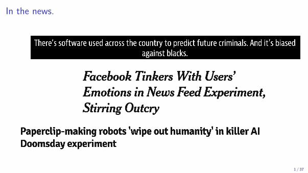
In the news.
1 / 37

Introduction• Algorithmic decision making in consequential settings:
Hiring, consumer credit, bail setting, news feed selection, pricing, ...
• Public concerns:Are algorithms discriminating?Can algorithmic decisions be explained?Does AI create unemployment?What about privacy?
• Taken up in computer science:
“Fairness, Accountability, and Transparency,”“Value Alignment,” etc.
• Normative foundations for these concerns?How to evaluate decision making systems empirically?
• Economists (among others) have debated related questionsin non-automated settings for a long time!
2 / 37
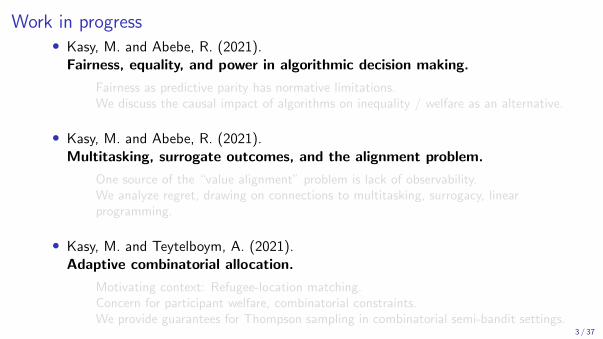
Work in progress• Kasy, M. and Abebe, R. (2021).
Fairness, equality, and power in algorithmic decision making.
Fairness as predictive parity has normative limitations.We discuss the causal impact of algorithms on inequality / welfare as an alternative.
• Kasy, M. and Abebe, R. (2021).Multitasking, surrogate outcomes, and the alignment problem.
One source of the “value alignment” problem is lack of observability.We analyze regret, drawing on connections to multitasking, surrogacy, linearprogramming.
• Kasy, M. and Teytelboym, A. (2021).Adaptive combinatorial allocation.
Motivating context: Refugee-location matching.Concern for participant welfare, combinatorial constraints.We provide guarantees for Thompson sampling in combinatorial semi-bandit settings.
3 / 37

Drawing on literatures in economics
• Social Choice theory.
How to aggregate individual welfare rankings into a social welfare function?
• Optimal taxation.
How to choose optimal policies
subject to informational constraints and distributional considerations?
• The economics of discrimination.What are the mechanisms driving inter-group inequality,
and how can we disentangle them?
• Labor economics, wage inequality, and distributional decompositions.
What are the mechanisms driving rising wage inequality?
4 / 37

Literatures in economics, continued
• Causal inference.
How can we make plausible predictions
about the impact of counterfactual policies?
• Contract theory, mechanism design, and multi-tasking.
What are the dangers of incentives based on quantitative performance measures?
• Experimental design and surrogate outcomes.
How can we identify causal effects if the outcome of interest is unobserved?
• Market design, matching and optimal transport.
How can two-side matching markets be organized without a price mechanism?
5 / 37
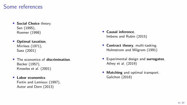
Some references
• Social Choice theory.Sen (1995),Roemer (1998)
• Optimal taxation.Mirrlees (1971),Saez (2001)
• The economics of discrimination.Becker (1957),Knowles et al. (2001)
• Labor economics.Fortin and Lemieux (1997),Autor and Dorn (2013)
• Causal inference.Imbens and Rubin (2015)
• Contract theory, multi-tasking.Holmstrom and Milgrom (1991)
• Experimental design and surrogates.Athey et al. (2019)
• Matching and optimal transport.Galichon (2018)
6 / 37

Introduction
Fairness, equality, and power in algorithmic decision makingFairnessInequality
Value alignment, multi-tasking, and surrogate outcomesMulti-tasking, surrogatesMarkov Decision Problems, Reinforcement learning
Adaptive combinatorial allocationMotivation: Refugee resettlementPerformance guarantee
Conclusion

Introduction
• Public debate and the computer science literature:Fairness of algorithms, understood as the absence of discrimination.
• We argue: Leading definitions of fairness have three limitations:
1. They legitimize inequalities justified by “merit.”
2. They are narrowly bracketed; only consider differencesof treatment within the algorithm.
3. They only consider between-group differences.
• Two alternative perspectives:
1. What is the causal impact of the introduction of an algorithm on inequality?
2. Who has the power to pick the objective function of an algorithm?
7 / 37

Fairness in algorithmic decision making – Setup
• Binary treatment W , treatment return M (heterogeneous), treatment cost c .Decision maker’s objective
µ = E [W · (M − c)].
• All expectations denote averages across individuals (not uncertainty).
• M is unobserved, but predictable based on features X .For m(x) = E [M|X = x ], the optimal policy is
w∗(x) = 1(m(X ) > c).
8 / 37
Examples
• Bail setting for defendants based on predicted recidivism.
• Screening of job candidates based on predicted performance.
• Consumer credit based on predicted repayment.
• Screening of tenants for housing based on predicted payment risk.
• Admission to schools based on standardized tests.
9 / 37

Definitions of fairness• Most definitions depend on three ingredients.
1. Treatment W (job, credit, incarceration, school admission).
2. A notion of merit M (marginal product, credit default, recidivism, test performance).
3. Protected categories A (ethnicity, gender).
• I will focus, for specificity, on the following definition of fairness:
π = E [M|W = 1,A = 1]− E [M|W = 1,A = 0] = 0
“Average merit, among the treated, does not vary across the groups a.”
This is called “predictive parity” in machine learning,the “hit rate test” for “taste based discrimination” in economics.
• “Fairness in machine learning” literature: Constrained optimization.
w∗(·) = argmaxw(·)
E [w(X ) · (m(X )− c)] subject to π = 0.
10 / 37
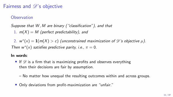
Fairness and D ’s objective
Observation
Suppose that W ,M are binary (“classification”), and that
1. m(X ) = M (perfect predictability), and
2. w∗(x) = 1(m(X ) > c) (unconstrained maximization of D ’s objective µ).
Then w∗(x) satisfies predictive parity, i.e., π = 0.
In words:
• If D is a firm that is maximizing profits and observes everythingthen their decisions are fair by assumption.
– No matter how unequal the resulting outcomes within and across groups.
• Only deviations from profit-maximization are “unfair.”
11 / 37
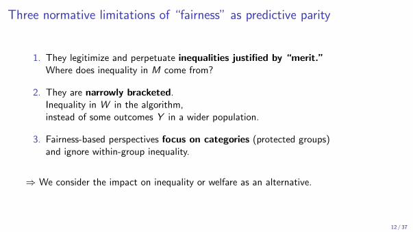
Three normative limitations of “fairness” as predictive parity
1. They legitimize and perpetuate inequalities justified by “merit.”Where does inequality in M come from?
2. They are narrowly bracketed.Inequality in W in the algorithm,instead of some outcomes Y in a wider population.
3. Fairness-based perspectives focus on categories (protected groups)and ignore within-group inequality.
⇒ We consider the impact on inequality or welfare as an alternative.
12 / 37
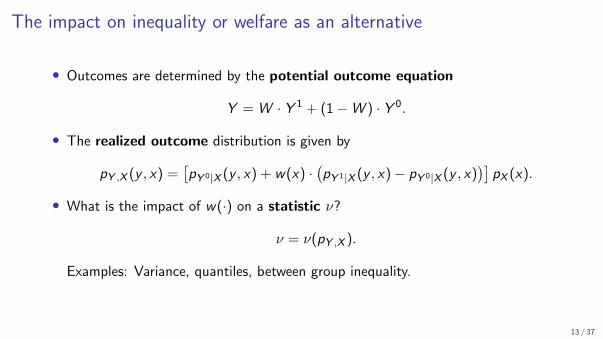
The impact on inequality or welfare as an alternative
• Outcomes are determined by the potential outcome equation
Y = W · Y 1 + (1−W ) · Y 0.
• The realized outcome distribution is given by
pY ,X (y , x) =[pY 0|X (y , x) + w(x) ·
(pY 1|X (y , x)− pY 0|X (y , x)
)]pX (x).
• What is the impact of w(·) on a statistic ν?
ν = ν(pY ,X ).
Examples: Variance, quantiles, between group inequality.
13 / 37
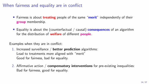
When fairness and equality are in conflict
• Fairness is about treating people of the same “merit” independently of theirgroup membership.
• Equality is about the (counterfactual / causal) consequences of an algorithmfor the distribution of welfare of different people.
Examples when they are in conflict:
1. Increased surveillance / better prediction algorithms:Lead to treatments more aligned with “merit”Good for fairness, bad for equality.
2. Affirmative action / compensatory interventions for pre-existing inequalities:Bad for fairness, good for equality.
14 / 37
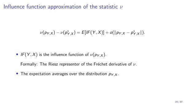
Influence function approximation of the statistic ν
ν(pY ,X )− ν(p∗Y ,X ) = E [IF (Y ,X )] + o(‖pY ,X − p∗Y ,X‖).
• IF (Y ,X ) is the influence function of ν(pY ,X ).
Formally: The Riesz representer of the Frechet derivative of ν.
• The expectation averages over the distribution pY ,X .
15 / 37

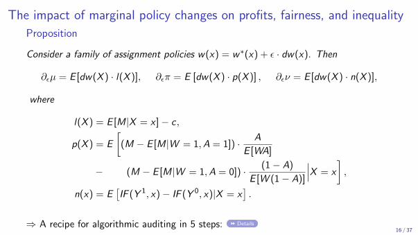
The impact of marginal policy changes on profits, fairness, and inequality
Proposition
Consider a family of assignment policies w(x) = w∗(x) + ε · dw(x). Then
∂εµ = E [dw(X ) · l(X )], ∂επ = E [dw(X ) · p(X )] , ∂εν = E [dw(X ) · n(X )],
where
l(X ) = E [M|X = x ]− c ,
p(X ) = E
[(M − E [M|W = 1,A = 1]) · A
E [WA]
− (M − E [M|W = 1,A = 0]) · (1− A)
E [W (1− A)]
∣∣∣X = x
],
n(x) = E[IF (Y 1, x)− IF (Y 0, x)|X = x
].
⇒ A recipe for algorithmic auditing in 5 steps: Details16 / 37

Power
• Both fairness and equality are about differences between peoplewho are being treated.
• Elephant in the room:• Who is on the other side of the algorithm?
• Who gets to be the decision maker D – who gets to pick the objective function µ?
• Political economy perspective:• Ownership of the means of prediction.
• Data and algorithms.
17 / 37

Introduction
Fairness, equality, and power in algorithmic decision makingFairnessInequality
Value alignment, multi-tasking, and surrogate outcomesMulti-tasking, surrogatesMarkov Decision Problems, Reinforcement learning
Adaptive combinatorial allocationMotivation: Refugee resettlementPerformance guarantee
Conclusion

The value alignment problem
• Much recent attention; e.g. Russell (2019):
[...] we may suffer from a failure of value alignment—we may, perhaps in-advertently, imbue machines with objectives that are imperfectly alignedwith our own
• The debate in tech & CS focuses on robotics and the grand, e.g. Bostrom (2003):
Suppose we have an AI whose only goal is to make as many paper clips aspossible. The AI will realize quickly that it would be much better if therewere no humans because humans might decide to switch it off. [...]
18 / 37
Value alignment and observability
• No need to wait for the singularity:There are many examples (outside robotics) in the social world, right now.
Social media feeds maximizing clicks.Teachers promoted based on student test scores.Doctors paid per patient....
• One unifying theme: Lack of observability of welfare.
• How to design
reward functions,incentive systems,adaptive treatment assignment algorithms,
when our true objective is not observed?
19 / 37

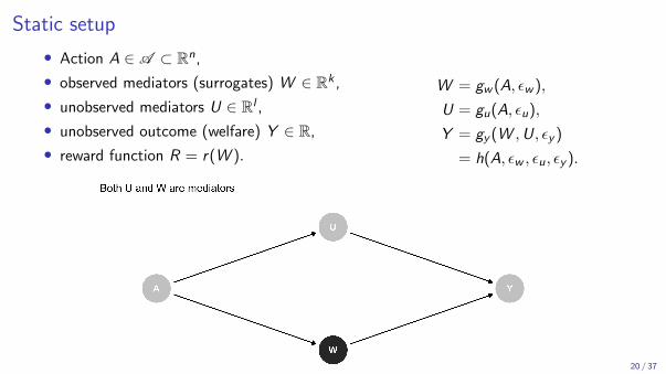
Static setup
• Action A ∈ A ⊂ Rn,
• observed mediators (surrogates) W ∈ Rk ,
• unobserved mediators U ∈ Rl ,
• unobserved outcome (welfare) Y ∈ R,
• reward function R = r(W ).
W = gw (A, εw ),
U = gu(A, εu),
Y = gy (W ,U, εy )
= h(A, εw , εu, εy ).
20 / 37
Static setup
• Action A ∈ A ⊂ Rn,
• observed mediators (surrogates) W ∈ Rk ,
• unobserved mediators U ∈ Rl ,
• unobserved outcome (welfare) Y ∈ R,
• reward function R = r(W ).
W = gw (A, εw ),
U = gu(A, εu),
Y = gy (W ,U, εy )
= h(A, εw , εu, εy ).
20 / 37

Mis-specified reward and regret
• We want to analyze algorithms that maximize the reward Rrather than true welfare Y .
• Expected welfare and expected reward:
y(a) = E [Y |do(A = a)] r(a) = E [R|do(A = a)]
(Using the do-calculus notation of Pearl 2000).
• Optimal and pseudo-optimal action:
a∗ = argmaxa∈A
y(a), a+ = argmaxa∈A
r(a).
• Regret:∆ = y(a∗)− y(a+).
21 / 37
Related literature 1: Multi-tasking
• Holmstrom and Milgrom (1991):Why are high-powered economic incentives rarely observed?
• Agent chooses effort A ∈ R2,to maximize their expectation of utility R,which depends on a monetary rewardthat in turn is a linear function of noisy measures of effort, (W1,W2).
22 / 37
Multi-tasking, continued
• In their model, the certainty equivalent of agent rewards equals
r(a) = α + β1a1 + β2a2 − C (a1 + a2)− 1
2r(β21σ
21 + β22σ
22
).
where C (·) is the increasing and concave cost of effort.
• ⇒ Positive effort aj on both dimension only if β1 = β2.
• If σj =∞ for one j (unobservable component),β1 = β2 = 0 for the optimal contract.
23 / 37

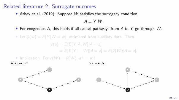
Related literature 2: Surrogate oucomes• Athey et al. (2019): Suppose W satisfies the surrogacy condition
A ⊥ Y |W .
• For exogenous A, this holds if all causal pathways from A to Y go through W .
• Let y(w) = E [Y |W = w ], estimated from auxiliary data. Then
y(a) = E [E [Y |A,W ]|A = a]
= E [E [Y | W ]|A = a] = E [y(W )|A = a].
• Implication: For r(W ) = y(W ), a+ = a∗!
24 / 37

Discrete actions, linear rewards• Suppose the set of feasible actions is finite.
• Allow for randomized actions.
A ∈
{a :
∑i
ai = 1, ai ≥ 0
}.
• Notation:• ej denote the unit vectors in Rk , p(w , a) = P(W = w |A = a),• y denotes the vector with elements y(ej), similarly for r ,
p denotes the matrix with elements p(w , ej),• ‖ · ‖∞ is the sup-norm.
• The best possible action and reward maximizing action are given by corners of thesimplex:
a∗ = e j∗ , j∗ ∈ argmaxj
yj ,
a+ = e j+ , j+ ∈ argmaxj
(r · p)j , ∆ = y(ej∗)− y(ej+).25 / 37

Bounding regret
Lemma
For arbitrary rewards r ,0 ≤ ∆ ≤ 2 · ‖y − r · p‖∞ .
Thus:
• For surrogate rewards r sur = y ,
∆ ≤ 2 · ‖y − y · p‖∞ .
• For optimal rewards ropt ∈ argmax r :‖r‖=1 yj+ ,
∆ ≤ 2 ·minr‖y − r · p‖∞ .
26 / 37

Dynamic version:Markov Decision Problems and Reinforcement Learning
• Sutton and Barto (2018); Francois-Lavet et al. (2018)).
• States s, actions a, transition probabilities p(s, a, s ′),and conditionally expected true rewards y(s, a).
• Probability x(s, a) of choosing action a.⇒ Markov process with stationary distribution π(s, a), average welfare
Vx = plimT→∞
1
T
T∑t=1
Y (ST ,AT ) =∑s,a
y(s, a)π(s, a).
• Two equivalent problems:Optimal policy x(s, a) ⇔ Optimal stationary distribution π(s, a).
27 / 37

Lemma (Linar programming formulation)
The optimal stationary distribution of the MDP is given by
π∗Y (·) = argmaxπ(·)
∑s,a
y(s, a) · π(s, a), subject to∑s,a
π(s, a) = 1, π(s, a) > 0 for all s, a.∑a
π(s ′, a) =∑s,a
π(s, a) · p(s, a, s ′) for all s ′ (1)
28 / 37
Mis-specified rewards in the dynamic setting
• Replacing y(s, a) with potentially misspecified expected rewards r(s, a)⇒ π+, with expected regret
∆ =∑s,a
y(s, a) ·(π∗(s, a)− π+(s, a)
).
• This is equivalent to the static linear setup,with the added constraint (1)!
29 / 37
Introduction
Fairness, equality, and power in algorithmic decision makingFairnessInequality
Value alignment, multi-tasking, and surrogate outcomesMulti-tasking, surrogatesMarkov Decision Problems, Reinforcement learning
Adaptive combinatorial allocationMotivation: Refugee resettlementPerformance guarantee
Conclusion
Motivation: Ethics of experimentation
• “Active learning” often involves experimentation in social contexts.
• This is especially sensitive when vulnerable populations are affected.
• (When) is it ethical to experiment on humans?
Kant (1791):
Act in such a way that you treat humanity, whether in your own personor in the person of any other, never merely as a means to an end, butalways at the same time as an end.
30 / 37
Combinatorial allocation problems
• Our motivating example:• Refugee resettlement in the US: By resettlement agencies (like HIAS).• Small number of slots in various locations.• Refugees without prior ties: Distributed pretty much randomly.• Alex Teytelboym’s prior work with HIAS, Annie MOORE:
Estimate refugee-location match effects on employment, using past data,find optimal matching, implement.
• This project: Learning while matching.
• Many policy problems have a similar form:• Resources / agents / locations get allocated to each other.• Various feasibility constraints.• The returns of different options (combinations) are unknown.• The decision has to be made repeatedly.
31 / 37
Sketch of setup
• There are J options (e.g., matches).
• Every period, our action is to choose at most M options.
• Before the next period, we observe the outcomes of every chosen option.
• Our reward is the sum of the outcomes of the chosen options.
• Our objective is to maximize the cumulative expected rewards.
Notation:
• Actionsa ∈ A ⊆ {a ∈ {0, 1}J : ‖a‖1 = M}.
• Expected reward:R(a) = E[〈a,Yt〉|Θ] = 〈a,Θ〉.
32 / 37

Thompson sampling
• Take a random action a ∈ A, sampled according to the distribution
Pt(At = a) = Pt(A∗t = a),
where Pt is the posterior at the beginning of period t.
• Introduced by Thompson (1933) for treatment assignment in adaptiveexperiments.
33 / 37
Regret bound
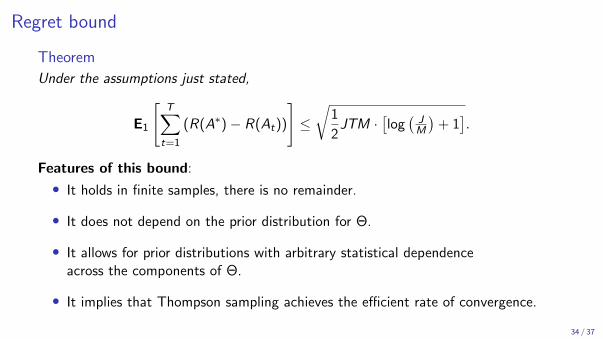
Theorem
Under the assumptions just stated,
E1
[T∑t=1
(R(A∗)− R(At))
]≤√
1
2JTM ·
[log(JM
)+ 1].
Features of this bound:
• It holds in finite samples, there is no remainder.
• It does not depend on the prior distribution for Θ.
• It allows for prior distributions with arbitrary statistical dependenceacross the components of Θ.
• It implies that Thompson sampling achieves the efficient rate of convergence.
34 / 37

Regret bound
Theorem
Under the assumptions just stated,
E1
[T∑t=1
(R(A∗)− R(At))
]≤√
1
2JTM ·
[log(JM
)+ 1].
Verbal description of this bound:
• The worst case expected regret (per unit) across all possible priorsgoes to 0 at a rate of 1 over the square root of the sample size, T ·M.
• The bound grows, as a function of the number of possible options J, like√J
(ignoring the logarithmic term).
• Worst case regret per unit does not grow in the batch size M,despite the fact that action sets can be of size
( JM
)!
35 / 37

Key steps of the proof
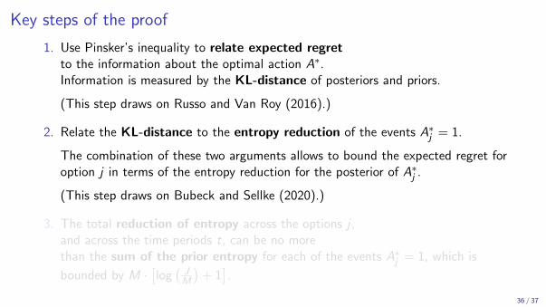
1. Use Pinsker’s inequality to relate expected regretto the information about the optimal action A∗.Information is measured by the KL-distance of posteriors and priors.
(This step draws on Russo and Van Roy (2016).)
2. Relate the KL-distance to the entropy reduction of the events A∗j = 1.
The combination of these two arguments allows to bound the expected regret foroption j in terms of the entropy reduction for the posterior of A∗j .
(This step draws on Bubeck and Sellke (2020).)
3. The total reduction of entropy across the options j ,and across the time periods t, can be no morethan the sum of the prior entropy for each of the events A∗j = 1, which is
bounded by M ·[log(JM
)+ 1].
36 / 37
Key steps of the proof
1. Use Pinsker’s inequality to relate expected regretto the information about the optimal action A∗.Information is measured by the KL-distance of posteriors and priors.
(This step draws on Russo and Van Roy (2016).)
2. Relate the KL-distance to the entropy reduction of the events A∗j = 1.
The combination of these two arguments allows to bound the expected regret foroption j in terms of the entropy reduction for the posterior of A∗j .
(This step draws on Bubeck and Sellke (2020).)
3. The total reduction of entropy across the options j ,and across the time periods t, can be no morethan the sum of the prior entropy for each of the events A∗j = 1, which is
bounded by M ·[log(JM
)+ 1].
36 / 37
Conclusion and summary
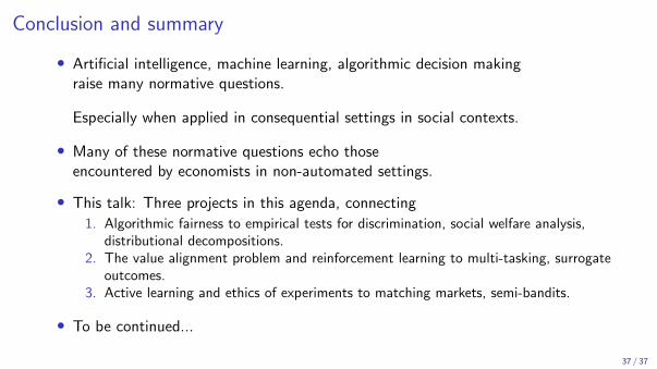
• Artificial intelligence, machine learning, algorithmic decision makingraise many normative questions.
Especially when applied in consequential settings in social contexts.
• Many of these normative questions echo thoseencountered by economists in non-automated settings.
• This talk: Three projects in this agenda, connecting
1. Algorithmic fairness to empirical tests for discrimination, social welfare analysis,distributional decompositions.
2. The value alignment problem and reinforcement learning to multi-tasking, surrogateoutcomes.
3. Active learning and ethics of experiments to matching markets, semi-bandits.
• To be continued...
37 / 37

Thank you!

A recipe for algorithmic auditing in 5 steps
1. Normative choices
• Relevant outcomes Y for individuals’ welfare?• Measures of welfare or inequality ν? Quantiles are a good default!
2. Calculation of influence functions
• At the appropriate baseline distribution,• evaluated for each (Yi ,Xi ), and stored in a new variable.
3. Causal effect estimation
• Estimate and impute n(x) = E[IF (Y 1, x)− IF (Y 0, x)|X = x
].
• E.g., assume W ⊥ (Y 0,Y 1)|X ,estimate n(·) using causal forest approach of Wager and Athey (2018).

A recipe for algorithmic auditing in 5 steps, continued
4. Counterfactual assignment probabilities
• Impute ∆w(xi ) = w(xi )− w∗(xi ) for all i in the sample.
5. Evaluation of distributional impact
• Calculate ∆ν = α · 1n∑
i ∆w(xi ) · n(xi ).
Back