the sparc data initiative: comparison of upper troposphere

The SPARC Data Initiative: Comparison of uppertroposphere/lower stratosphere ozone climatologiesfrom limb-viewing instruments and the nadir-viewingTropospheric Emission SpectrometerJ. L. Neu1, M. I. Hegglin2, S. Tegtmeier3, A. Bourassa4, D. Degenstein4, L. Froidevaux1, R. Fuller1,B. Funke5, J. Gille6, A. Jones7, A. Rozanov8, M. Toohey3, T. von Clarmann9, K. A. Walker7,and J. R. Worden1

1Jet Propulsion Laboratory, California Institute of Technology, Pasadena, California, USA, 2Department ofMeteorology, Universityof Reading, Reading, UK, 3GEOMAR Helmholtz Centre for Ocean Research, Kiel, Germany, 4Department of Physics andEngineering Physics, University of Saskatchewan, Saskatoon, Saskatchewan, Canada, 5Instituto de Astrofisica de Andalucia, CSIC,Granada, Spain, 6Department of Oceanic and Atmospheric Sciences, University of Colorado Boulder, Boulder, Colorado, USA,7Department of Physics, University of Toronto, Toronto, Ontario, Canada, 8Department of Physics and Electrical Engineering,University of Bremen, Bremen, Germany, 9Department of Physics, Karlsruhe Institute of Technology, Karlsruhe, Germany

Abstract We present the first comprehensive intercomparison of currently available satellite ozoneclimatologies in the upper troposphere/lower stratosphere (UTLS) (300–70 hPa) as part of theStratosphere-troposphere Processes and their Role in Climate (SPARC) Data Initiative. The TroposphericEmission Spectrometer (TES) instrument is the only nadir-viewing instrument in this initiative, as well as the onlyinstrument with a focus on tropospheric composition. We apply the TES observational operator to ozoneclimatologies from the more highly vertically resolved limb-viewing instruments. This minimizes the impact ofdifferences in vertical resolution among the instruments and allows identification of systematic differences inthe large-scale structure and variability of UTLS ozone. We find that the climatologies from most of thelimb-viewing instruments show positive differences (ranging from 5 to 75%) with respect to TES in thetropical UTLS, and comparison to a “zonal mean” ozonesonde climatology indicates that these differenceslikely represent a positive bias for p≤ 100 hPa. In the extratropics, there is good agreement among theclimatologies regarding the timing andmagnitude of the ozone seasonal cycle (differences in the peak-to-peakamplitude of <15%) when the TES observational operator is applied, as well as very consistent midlatitudeinterannual variability. The discrepancies in ozone temporal variability are larger in the tropics, with differencesbetween the data sets of up to 55% in the seasonal cycle amplitude. However, the differences among theclimatologies are everywhere much smaller than the range produced by current chemistry-climate models,indicating that the multiple-instrument ensemble is useful for quantitatively evaluating these models.

1. Introduction

Ozone is the third largest component of radiative forcing [Solomon et al., 2007], with maximum radiativeeffect in the upper troposphere and lower stratosphere (UTLS) [Forster and Shine, 2002]. Yet the processesthat control the UTLS distribution of ozone and its trends and variability, including the exchange of airbetween the stratosphere and troposphere, are not well quantified [World Meteorological Organization, 2011].The UTLS region is characterized by strong vertical and horizontal ozone gradients and complex and rapidlyevolving small-scale features such as tropopause folds [Gettelman et al., 2011, and references therein]. Aircraftmeasurements are well suited for characterizing UTLS chemistry and dynamics because of their high spatialand temporal resolution. However, aircraft have only sparsely sampled the UTLS, raising questions about therepresentativeness of these measurements for applications such as evaluating free-running global chemistry-climate models [Stratosphere-troposphere Processes and their Role in Climate Chemistry-Climate Model Validation(SPARC CCMVal), 2010; Hegglin et al., 2010]. Current satellite instruments lack the spatiotemporal resolutionto resolve some UTLS features, such as thin, highly dynamic filaments. Furthermore, they can have low signal-to-noise in the UTLS because of the small ozone abundance there relative to the middle stratosphere, andclouds can interfere with trace gas retrievals. However, satellites provide much greater spatial and temporal

NEU ET AL. ©2014. American Geophysical Union. All Rights Reserved. 6971

PUBLICATIONSJournal of Geophysical Research: Atmospheres

RESEARCH ARTICLE10.1002/2013JD020822

Special Section:The SPARC Data Initiative –Intercomparison of VerticallyResolved Chemical Trace Gasand Aerosol Climatologies

Key Points:• First comprehensive intercomparisonof UTLS ozone climatologies

• Compares climatologies from limbsounders to the TES nadir sounder

• Accounts for differences invertical resolution

Correspondence to:J. L. Neu,[email protected]

Citation:Neu, J. L., et al. (2014), The SPARC DataInitiative: Comparison of uppertroposphere/lower stratosphere ozoneclimatologies from limb-viewinginstruments and the nadir-viewingTropospheric Emission Spectrometer,J. Geophys. Res. Atmos., 119, 6971–6990,doi:10.1002/2013JD020822.

Received 4 SEP 2013Accepted 28 APR 2014Accepted article online 4 MAY 2014Published online 12 JUN 2014

http://publications.agu.org/journals/

http://onlinelibrary.wiley.com/journal/10.1002/(ISSN)2169-8996

http://dx.doi.org/10.1002/2013JD020822

http://dx.doi.org/10.1002/2013JD020822

http://onlinelibrary.wiley.com/journal/10.1002/(ISSN)2169-8996/specialsection/SPARC1




coverage than aircraft, at a vertical resolution that is commensurate with that of most models [SPARC CCMVal,2010;Hegglin et al., 2010], and their measurements have provided extensive improvements in our understandingof UTLS structure and processes [e.g., Hegglin et al., 2009; Manney et al., 2011; Peevey et al., 2012].

The purpose of the SPARC Data Initiative (M. I. Hegglin and S. Tegtmeier, SPARC Data Initiative report on theevaluation of trace gas and aerosol climatologies from satellite limb sounders, manuscript in preparation,2014; M. I. Hegglin et al., SPARC Data Initiative: A multi-instrument comparison of stratospheric limbmeasurements, manuscript in preparation, Journal of Geophysical Research, 2014) is to better understandthe differences between measurements of stratospheric trace gases and aerosols from different satelliteinstruments in order to reduce uncertainties in model evaluations, trends, and process studies. Tegtmeieret al. [2013] provides a detailed description and comparison of the ozone climatologies from limb-viewinginstruments submitted to the Data Initiative, with a primary focus on the stratosphere. Here we compare theclimatologies from six limb-viewing instruments (Atmospheric Chemistry Experiment-Fourier TransformSpectrometer (ACE-FTS), Aura-Microwave Limb Sounder (MLS), High Resolution Dynamics Limb Sounder(HIRDLS), Michelson Interferometer for Passive Atmospheric Sounding (MIPAS), Optical Spectrograph andInfrared Imager System (OSIRIS), and Scanning Imaging Absorption Spectrometer for Atmospheric Chartography(SCIAMACHY)), with vertical ranges that extend into the UTLS, to those from the nadir-viewing TroposphericEmission Spectrometer (TES) instrument over 300–70hPa for 2005–2010. The TES instrument is focused ontropospheric composition. Its ozone measurements have good sensitivity from the surface to 10hPa and arewell validated against ozonesondes in the UTLS [Nassar et al., 2008; Boxe et al., 2010], as discussed in section 2.1.BecauseTES is nadir viewing, it has relatively coarse vertical resolution (~6–7 km) compared to the limb-viewinginstruments discussed here, most of which have vertical resolution of ~2–4 km. While TES has much finerhorizontal resolution (<10 km) than the limb sounders (~200 km), the spacing between measurements is182 km; thus, its ability to resolve horizontal features is not much different than that of the limb sounders.

Assessing the differences between satellite measurements in the UTLS is critical to advancing ourunderstanding of this region and evaluating UTLS processes in models because uncharacterized biases insatellite data can lead to incorrect conclusions about UTLS chemistry or radiative forcing. However, given thestrong gradients and small-scale structure of trace gas fields in the UTLS, differences in sampling and invertical and horizontal resolution among instruments can lead to large differences that reflect sampling orsmoothing error rather than systematic bias. Toohey et al. [2013] addresses the issue of sampling bias andshows, for example, that the construction of the zonal mean climatologies used here leads to biases of a fewpercent in the subtropical jet regions (~30°N and S) due to a combination of the sloping ozone surfaces inthese regions and the increase in sampling density with latitude. To address differences in verticalresolution, one approach is to smooth the measurements to a common resolution, which allows for an“apples-to-apples” comparison [Rodgers and Connor, 2003]. Here we use the TES observational operator(averaging kernel + constraint) to vertically smooth the climatologies from the limb sounders and provide acommon basis for assessment of systematic differences in large-scale vertical and horizontal gradients aswell as seasonal and interannual variability of ozone within the UTLS.

We use TES data as the common reference because TES ozone data have been extensively validated againstozonesondes for a wide range of geophysical states and latitudes. Studies have shown that there are noobservable changes in biases in the TES ozone data over time, and the bias is well characterized as a functionof latitude [Worden et al., 2007; Verstraeten et al., 2013]. In addition, the sonde comparisons indicate that thecalculated random errors are in agreement with actual errors. This means that evaluating other satellitemeasurements against TES provides an assessment of instrument bias rather than unquantified errors in theTES retrieval.

TES measures over the entire wavelength range of ozone infrared absorption and can thus provide thesensitivity of outgoing longwave radiation (OLR) to the vertical distribution of ozone [Worden et al., 2008,2011]. As part of the Atmospheric Chemistry and Climate Model Intercomparison Project (ACCMIP) TEStropospheric ozone and its effect on OLR have been compared to the same quantities derived from modelsand used to reduce uncertainties in ozone radiative forcing [Bowman et al., 2013]. TES is also extensively usedfor the evaluation of upper tropospheric ozone and its precursors in chemistry transport models [e.g., Joneset al., 2009]. Assessing the differences between TES and other instruments measuring ozone in the UTLSregion will provide a better understanding of the ozone gradients and variability that TES fails to capture due

Journal of Geophysical Research: Atmospheres 10.1002/2013JD020822


to its coarse resolution. Furthermore, improved characterization of satellite measurements of ozone in thisregion will allow us to better quantify the significance ofmodel-measurement differences in precursor emissionsand radiative forcing in the UTLS.

2. Data

Detailed information on the limb-viewing satellite instruments used here (ACE-FTS, Aura-MLS, HIRDLS, MIPAS,OSIRIS, and SCIAMACHY) can be found inM. I. Hegglin et al. (manuscript in preparation, 2014), while Tegtmeieret al. [2013] provide a discussion of their ozonemeasurements and SPARC Data Initiative ozone climatologies.The data versions used here are the same as those in Tegtmeier et al. [2013] (Table 1). The climatologiesconsist of zonal monthly mean ozone abundances for 36 latitude bins (midpoints at 87.5°S, 82.5°S,…, 87.5°N)calculated on a standard pressure grid, with 11 levels where p≥ 70 hPa (300, 250, 200, 170, 150, 130, 115, 100,90, 80, and 70 hPa). Toohey et al. [2013] and Funke and von Clarmann [2012] discuss potential errors inconstructed climatologies due to differences in instrument sampling and averaging technique, respectively.

2.1. TES Ozone Measurements

TES is a Fourier transform spectrometer that was launched on the NASA Earth Observing System Aura satellite in2004 [Beer, 2006; Beer et al., 2001]. The Aura satellite is in a Sun-synchronous polar orbit with equator crossingtimes of ~13:43 (ascending node) and ~1:43 (descending node) and a 16day repeat cycle. TES measures in thethermal infrared (650–3050 cm�1) with a spectral resolution of 0.06 cm�1 and provides line-width-limiteddiscrimination of radiatively active species, including O3, CO, H2O, HDO, CH4, CO2, NH3, CH3OH, and HCOOH,with greatest sensitivity in the troposphere. At the nadir, the horizontal resolution is 0.5 × 5 km, and the footprintis 5.3× 8.5 km, with a separation of ~182 km between consecutive measurements. In cloud-free conditions, TESnadir ozone profiles have approximately 4 degrees of freedom for signal, with ~2 in the troposphere and ~2 inthe stratosphere (below~5hPa), equivalent to a vertical resolution of ~6–7 km (Figure 1a). While TESmeasures inboth Global Survey and Special Observations modes, here we use only global survey data, which provide near-global coverage in 16 orbits (~26h). The retrievals and error estimation are based on the optimal estimationapproach [Rodgers, 2000] and are described inWorden et al. [2004], Bowman et al. [2002, 2006], and Kulawik et al.[2006]. TES data, including averaging kernels and error covariance matrices, are publicly available. For moreinformation, see http://tes.jpl.nasa.gov/.

We use TES data covering the period July 2005 to December 2010. TES provides global coverage from July2005 through May 2008. To extend the life of the instrument, the latitudinal coverage was reduced in June2008 to 60°S–82°N and in July 2008 to 50°S–70°N. From January to April 2010, the instrument went offlinedue to problems with the scanning mechanism. When operations resumed in May 2010, the latitudecoverage was further reduced to 30°S–50°N and the calibration strategy was changed to reduce wear on thepointing mechanism of the instrument. Reducing the number of calibration scans resulted in a 25% increasein the number of observations per global survey and regular but nonuniform spacing between themeasurements (ground track separation cycles through 56 km, 195 km, 187 km, and 122 km and then returnsto 56 km), with no discernible impact on data quality [e.g., Verstraeten et al., 2013]. A second data gap of~ 3weeks occurred in October 2010, with only two Global Surveys conducted that month.

The TES SPARC Data Initiative ozone climatology is based on Level 2 version 4 (V4) data [Boxe et al., 2010].Vertical profiles are retrieved as log(vmr), where vmr is volume mixing ratio, on a 67 Level pressure grid, andare interpolated in log(pressure) to the SPARC Data Initiative pressure grid. Only retrievals that pass themaster quality flag have been used, and there is an additional screening to eliminate “C curve” ozone profiles.

Table 1. Information on Limb-Viewing Instrumentsa

Instrument and Data Version Vertical Range Vertical Resolution References

ACE-FTS v2.2 update 5–95 km 3–4 km Dupuy et al. [2009]Aura-MLS v2.2 12–75 km 3 km Froidevaux et al. [2008] and Jiang et al. [2007]HIRDLS v6.0 10–55 km 1 km Nardi et al. [2008] and Gille et al. [2008]MIPAS v220 6–70 km 2.7–3.5 km von Clarmann et al. [2009]OSIRIS v5-0 10–60 km 2 km Degenstein et al. [2009]SCIAMACHY v2.5 10–60 km 3–5 km Mieruch et al. [2012]

aData version, vertical range, vertical resolution, and references for the six limb-viewing instruments used in this study.



http://tes.jpl.nasa.gov/

These profiles, which represent approximately 1–2%of TES V4 ozone data, result from nonlinearities inthe retrieval in the presence of clouds. Thesenonlinearities can lead to convergence to anunphysical state in which the ozone profile takeson a “C” shape under particular thermal conditions.While we do not perform any cloud screening inthe selection of profiles for the climatology, themaster quality flag does screen out profiles withcloud optical depth> 50 from 975 to 1200 cm�1.

TES measurements are retrieved, and thustypically averaged in, log-space. However, forproper comparison to other data sets shown here,we have used linear averaging. Simpleunweighted means of the available data arecalculated for each month and latitude bin. Aminimum of five observations per bin is required,but in practice the minimum number of profiles is28, and in most cases the number is >1000.

TES ozone measurements have been extensivelyvalidated against ozonesondes [Nassar et al., 2008;Boxe et al., 2010; Verstraeten et al., 2013]. In the300–70 hPa region evaluated here, TES ispositively biased with respect to sondes in alllatitude regions except the southern low andmiddle latitudes (15–60°S), where it is negativelybiased. The mean bias is smaller than 20% in alllatitude regions. In the northern midlatitudes, thebias is +15–20% for 100 hPa< p< 300 hPaand<+5% for 70 hPa< p< 100 hPa. The biascurve is “c shaped” in the southern midlatitudeUTLS, with near-zero bias at 300 and 70 hPa and amaximum value of �20% at 150 hPa. In thetropical UTLS, TES shows a small positive bias(<10%) with respect to sondes. An analysis ofseasonal variations in the northern midlatitude(35–56°N) bias showed relatively small seasonaldifferences, except during summer when the biasdecreases to <10% everywhere. In this paper, weinclude a comparison of the SPARC Data Initiativeclimatologies to a “zonal mean” ozonesondeclimatology (sections 3.4 and 3.5) and finddifferent biases for the TES climatology than those

reported in the TES validation literature in some regions. These differences likely result from not accountingfor (1) the sampling locations of the ozonesonde profiles and (2) the difference in vertical resolution betweenTES and the sondes in the climatological comparisons.

2.2. Use of Zonal Mean Monthly Mean Averaging Kernels

As discussed above, TES retrievals use the optimal estimation technique, with the retrieved profile, x̂ (ln(vmr)),given by the following:

x̂ ¼ xa þ Axx x � xað Þwhere x (ln(vmr)) is the true state, xa (ln(vmr)) is the a priori profile, and Axx is the averaging kernel matrix. Forthe comparisons shown here, the climatologies of the higher vertical resolution limb-viewing instruments are

-50 0 50Latitude

300

100

70

Pre

ssur

e(hP

a)

Influence of TES a priori on x, MIPAS 2008

150

200

a)

b)

Figure 1. (a) Sample TES averaging kernel. The lines show therelative contribution of the true mixing ratio at each pressurelevel to the retrieved mixing ratio at 500–1000hPa (green),100–500hPa (blue), and 10–100hPa (purple). TES ozone aver-aging kernels vary with temperature, surface properties, clouds,and ozone. (b) Influence of the TES a priori on the virtual retrievalfor MIPAS. Annual mean value of the ratio of Ax, the contributionof the original climatology to the virtual retrieval, to xa�Axa, thecontribution of the TES a priori to the virtual retrieval, for MIPASfor 2008. Results are very similar for other instruments and years.When the ratio is close to 1, the terms are of similar magnitudeso that the a priori and true profiles contribute equally to theretrieved ozone. Contour values of 1, 10, and 20 are shown.



taken to be the “true” state, x, and the TES observational operator (a priori and averaging kernel) are used tosimulate a “virtual” TES retrieval, x̂. Normally, this type of comparison is done on a profile-by-profile basis.However, due to the large number of instruments involved in this comparison and the focus on zonal meanclimatologies, we apply the monthly mean zonal mean observational operator to the monthly mean zonalmean SPARC Data Initiative climatologies. The use of monthly mean zonal mean averaging kernels can bejustified by the fact that the variations in TES averaging kernels are not highly correlated with variations inozone. In the troposphere, ozone explains less than 25% of the variance in the averaging kernel diagonal at alllatitudes due to the strong dependence of the averaging kernels on clouds, water vapor, and temperature, asdiscussed by Aghedo et al. [2011]. In the UTLS region, ozone explains up to 35% of the variance in theaveraging kernel diagonal in midlatitudes, with a minimum value at ~150–200 hPa where the sensitivity isrelatively low and the a priori has a significant impact on the retrievals (see below). In the tropical UTLS,ozone explains 20–60% of the variance in the averaging kernel diagonal, with maximum correlation at~150 hPa. However, at all latitudes the dependence of the averaging kernel diagonal on ozone abundance isweak for ozone within 40% of the mean value at each level; the correlations are primarily driven by ozoneabundances more than 40% higher than the mean value. In the midlatitudes, ozone abundances that aretwice as large as the mean value at a given pressure level have a ~30% higher averaging kernel diagonalvalue. In the tropics the slope of the relationship is somewhat higher, and a 100% increase in ozone over themean value is associated with a 45% larger averaging kernel diagonal.

Aghedo et al. [2011] examined the error associated with using monthly mean averaging kernels in twoclimate models for p ≥ 100 hPa. They found differences in ozone of at most 3% when using monthlymean as compared to time-varying averaging kernels. To test the error involved in using zonal meanaveraging kernels with zonal mean data, we examined the difference between TES and Aura-MLSmeasurements for 2006 gridded at 5° × 10°, using the 5° × 10° gridded TES averaging kernels to smooththe Aura-MLS measurements. The zonal mean of this difference is always within 10% of the differencebetween zonal mean TES and Aura-MLS measurements using zonal mean averaging kernels, andfurthermore, the difference in the zonal mean data sets is always less than the difference in gridded datasets except in high southern latitudes during October. In addition, the difference between using zonalmean averaging kernels aggregated from individual profiles and using the zonal mean of the griddedaveraging kernels is negligible (<2% everywhere). We therefore conclude that using zonal mean averagingkernels with zonal mean data provides a lower estimate that is within ~10%of the true difference between eachinstrument and TES. However, we note that because the averaging kernels are not fully independent of theozone abundance, comparison using the TES observational operator may not accurately reflect the differencebetween TES and another instrument if there are large systematic differences between them. Given the factthat the averaging kernels depend only weakly on the ozone abundance for ozone within 40% of the meanvalue, we do not expect this to be an issue except where instruments differ from TES bymore than 40%. In suchcases, which are rare (see the discussion of Figure 4 below), the error associated with using an averaging kernelthat has sensitivity that is not appropriate for the ozone observed by the other instrument can only bequantified by recalculating the averaging kernel to “match” the instrument’s ozone, which is beyond the scopeof this paper.

2.3. Applying the TES Observational Operator

For each instrument, we interpolate the monthly mean zonal mean climatologies from the SPARC pressuregrid to the TES retrieval levels (67 levels between the surface and 0.1 hPa). We fill in the levels below thelowest measurement in each latitude bin using the monthly mean, zonal mean TES a priori as a “fill profile.”The virtual TES retrievals are calculated and then interpolated back to the SPARC pressure grid, and weaverage over all of the available data from 2005 to 2010 to create the climatologies shown here. We use the apriori as a fill profile because it makes A(x� xa) = 0 in the troposphere (defined as p≥ pmax for eachinstrument) since x= xa there, which is equivalent to applying the observational operator only to the levelswhere the limb-viewing instruments provide measurements. However, the fill profile can still impact thecomparison to TES due to the vertical smearing of the averaging kernels. The difference between the virtualretrieval for a given instrument (x̂ INST) and TES (x̂TES) can be written as

x̂ INST � x̂TES ¼ ASS xSTRATTrue � xSTRATINST

� �� AST xTROPTrue � xTROPINST

� �



where ASS is the “stratospheric” component of the averaging kernel matrix (p< pmax), xSTRATINST is the ozoneprofile measured by the limb-viewing instrument, AST represents the cross terms of the averaging kernelthat define the tropospheric influence on the stratosphere, and xTROPINST is the fill profile. To test the sensitivityof our results to our approach of using the TES a priori to fill in the profiles below the lowest measurementlevel, we have also calculated virtual retrievals in which we scale the TES a priori using the percentdifference between the ozone value at pmax for each latitude bin for each of the other instruments andthe TES a priori at this same latitude and pressure. Comparison of the virtual retrievals using the twodifferent filling methods allows us to identify regions where our results are highly dependent on ourassumptions for p> pmax, as discussed below.

3. Intercomparison of Zonal Mean Ozone Climatologies

As in Tegtmeier et al. [2013], we use a series of diagnostics to evaluate differences in the vertical, latitudinal,and temporal structure of ozone as represented by the SPARC Data Initiative climatologies. These diagnosticsinclude zonal mean cross sections, vertical and latitudinal profiles, seasonal cycles, and interannual variability.However, rather than examining differences from the multi-instrument mean, we use the TES climatology asthe standard to which the other climatologies are compared and, in some cases, include climatologicalozonesonde measurements as an additional validation tool. We also analyze the impact of the TESobservational operator on the climatologies from the limb-viewing instruments and assess how the use ofthe observational operator affects the ozone intercomparison.

3.1. Zonal Mean Cross Sections

Figure 2 (left) shows the zonal mean ozone climatology for each instrument from 300 to 70hPa averaged over2005–2010 (2005–2007 for HIRDLS) using the data directly from the SPARC Data Initiative archive. All of theinstruments show similar features, including the typical low tropical values, strong subtropical gradients, andrelatively flat midlatitude isopleths that reflect the competing effects of the stratospheric overturning circulationandmixing with the troposphere. The instruments also all show lower ozone values in the Southern Hemispherethan in the Northern Hemisphere in the annual mean due to the asymmetry in the overturning circulation. Afew instruments show features not seen in the climatologies from any of the other instruments. The MIPASclimatology has an unusual contour shape in the tropics between ~200 and 100hPa, with a slight “double ear”structure in the subtropics and a deep minimum near the equator, and Aura-MLS has very flat, tightly spacedcontours near 100hPa. It is likely that some of the differences in the climatologies in the upper tropicaltroposphere arise from differences in the impact of clouds on the retrievals and in criteria used for cloudscreening, which can cause sampling artifacts (T. von Clarmann, personal communication, 2013). The OSIRISclimatology has an unusually strong zonal gradient at ~75°N below 250hPa, which appears to reflect samplingbias in the climatology resulting from a lack of measurements in polar winter [Toohey et al., 2013].

3.2. Impact of TES Observational Operator

Figure 2 (middle) shows the virtual retrievals using the TES observational operator, and Figure 2 (right) showsthe percent difference between the virtual TES retrieval (VTR) and the original climatology (OC) for eachinstrument (100 × (VTR�OC)/OC). Hatched regions in Figure 2 (right) indicate where the choice of fill profile(TES a priori or scaled a priori) has a significant impact on the VTR, quantified (arbitrarily) as where thedifference between the VTRs using the two fill profiles exceeds 10%. The HIRDLS climatology shows the mostuniform and smallest changes in ozone after the application of the TES observational operator. The operatoracts to smooth out the small-scale features seen in the MIPAS, Aura-MLS, and OSIRIS climatologies, as seen inFigure 2 (middle), due to the vertical smearing of the broad averaging kernels. In the tropics, theobservational operator tends to increase ozone for p≤ 80 hPa and decrease it for p> 80 hPa relative to theoriginal climatologies (with strong increases at 100 hPa associated with the unusual features in MIPAS andAura-MLS). MIPAS and Aura-MLS are the only two instruments for which the choice of the fill profile has asignificant impact in the tropics. It is unclear why this is the case for Aura-MLS, but the MIPAS tropical ozonevalues are very low at p> 250 hPa compared to the other instruments, and there is a very large differencebetween the TES a priori and the a priori scaled using the MIPAS measurements in this region.

In the extratropics, the observational operator tends to increase ozone at ~150 hPa and decrease it above andbelow, which increases the vertical and horizontal gradients of ozone in the virtual retrievals compared to the



Figure 2. Cross sections of annual mean zonal mean ozone from 300 to 70hPa for 2005–2010. (left) Ozone cross sections fromACE-FTS, Aura-MLS, HIRDLS (2005–2007), MIPAS, OSIRIS, SCIAMACHY, and TES. (middle) Cross sections from ACE-FTS, Aura-MLS,HIRDLS, MIPAS, OSIRIS, and SCIAMACHY after application of the TES observational operator. (right) Percent change in annualmean zonal mean ozone introduced by the TES observational operator (100× (VTR�OC)/OC, where VTR=virtual TES retrievaland OC=original climatology). Hatching indicates regions where the difference between the virtual retrievals using the TES apriori as the fill profile and those using the scaled a priori as the fill profile exceeds 10%. See text for details.



original climatologies. This increase in gradient clearly cannot result from the TES averaging kernels, whichsmooth and flatten vertical gradients. Rather, the increase results from the influence of the a priori;comparison of the terms Ax, the contribution of the true profile from each climatology to the virtual retrieval,and xa� Axa, the contribution of the TES a priori to the virtual retrieval, (Figure 1b) shows that TES’s sensitivityis lowest, and the a priori profile makes the largest contribution to x̂ , in the midlatitudes at ~150–200 hPa, aswell as in the southern high latitudes at p> 150 hPa.

Figure 3. Vertical profiles of zonal mean ozone for 2005–2010. (left column) Ozone profiles from the original clima-tology for each instrument. (middle column) Ozone profiles after application of the TES observational operator. TESmeasurements are the same as in the Figure 3 (left column). (right column) The percent change in the ozoneprofiles introduced by the TES observational operator for all instruments except TES (100 × (VTR�OC)/OC). Dashedlines indicate portions of the profile where the difference between the virtual retrievals using the TES a priori as thefill profile and those using the scaled a priori as the fill profile exceeds 10%. (top row) Zonal mean ozone profilesand differences for 40–45°N for April 2005–2010. (middle row) Annual mean zonal mean ozone profiles anddifferences for 5°S–5°N for 2005–2010. (bottom row) Zonal mean ozone profiles and differences for 40–45°S forOctober 2005–2010.



The sensitivity to the fill profile is largestin the extratropics, in particular for theclimatologies whose range does notextend to 300 hPa (Aura-MLS, OSIRIS,and SCIAMACHY). Between ~200 and300 hPa there are large vertical gradientsin midlatitude ozone that are not wellrepresented by the TES a priori so thatthere is a large difference between thetwo fill profiles (the a priori and thescaled a priori). Furthermore, theaveraging kernels spread theinformation from 300 hPa upward to~100 hPa in the extratropics so thatchanging ozone at 300 hPa has asignificant influence over a largevertical range.

Figure 3 shows a comparison of zonalmean vertical profiles in the northernmidlatitudes (April), tropics (annual mean),and southern midlatitudes (October).Figure 3 (left column) is once again theoriginal SPARC Data Initiative climatologyfor each instrument, while Figure 3(middle and right columns) show thevirtual retrievals using the TES observationoperator and the percent differencebetween the virtual retrievals and theoriginal data (100× (VTR�OC)/OC),respectively. Dashed lines in Figure 3(right column) indicate where thechoice of fill profile affects the VTR bymore than 10%. In the midlatitudes,the observational operator smoothesthe vertical profiles; it decreases ozonefor p> 150 hPa and increases it forp< 150hPa for all instruments for whichthe virtual retrievals do not dependstrongly on the fill profile. In the tropics,as discussed above, the observationaloperator acts to slightly increase ozone atp< 80hPa and slightly decrease it atp> 80hPa, as well as to smooth small-scale vertical structures.

3.3. Percent Difference From TES

Figure 4 shows the percent differencebetween the annual mean climatologyfor each instrument and TES(100 × (OC� TES)/TES, left) and thepercent difference between the virtualretrievals for each instrument and TES(100 × (VTR-TES)/TES, Figure 4, right).

Figure 4. Cross sections of annual mean zonal mean ozone differencesfrom 300 to 70 hPa for 2005–2010. (left) Annual mean zonal meanozone percent differences between the climatology from each instru-ment and TES for 2005–2010 (HIRDLS: 2005–2007) (100× (OC� TES)/TES).(right) Percent differences between the virtual retrieval from eachinstrument and TES after application of the TES observational operator(100× (VTR� TES)/TES). Hatched regions indicate where the difference inthe virtual retrieval using the two different fill profiles exceeds 50% of thedifference between the virtual retrieval and TES.



The hatched regions in Figure 4 (right) indicate where differences in the VTR due to the choice of fill profileexceed 50% of the difference between the VTR and TES for each instrument. While 50% is an arbitrarychoice, it highlights a combination of regions where the fill profile has a >10% impact on the virtualretrievals (see Figure 2 above) and regions where differences between the virtual retrievals and TES aresmall so that even <10% differences due to the fill profile are large relative to VTR-TES. The originalclimatologies from all instruments except ACE-FTS and OSIRIS show positive differences of more than 25%with respect to TES in the tropics. However, except for HIRDLS, which is affected by uncorrected emissionfrom aerosols in the tropics (J. Gille, private communication, 2013), the biases are not uniform in pressure,and there are some regions with negative biases, including for p< 70 hPa (which can impact the region ofinterest when the TES observational operator is applied). The virtual retrievals represent the combinedinfluence of the vertical smoothing of the TES averaging kernel and the a priori, whose influence is notnegligible due to TES’s imperfect sensitivity. Together these act to both vertically smooth the differencesfrom TES and reduce them to≤ 25% for the virtual retrievals from all instruments except HIRDLS. However,for the Aura-MLS and MIPAS virtual retrievals, the biases with respect to TES are robust (i.e., not stronglydependent on the fill profile) only for p<~100 hPa. For ACE-FTS, which is a solar occultation instrumentand has very sparse sampling in the tropics due to its orbit, the difference from TES may largely reflect a>5% tropical sampling bias in the climatology [Toohey et al., 2013].

HIRDLS andMIPAS also have annual mean positive differences of 10–30%with respect to TES at p≥ 150 hPa inthe northern middle and high latitudes. Again, the differences with respect to TES can be seen in the originalclimatologies, but the vertical extent of the positive biases is greater in the virtual retrievals. The climatologiesfrom the other instruments also show positive differences from TES in the same region, but for the most partthese are not seen in the original climatologies and are an artifact of the impact of the fill profile. In theSouthern Hemisphere, the original climatologies are generally negatively biased with respect to TES,especially above 200 hPa. The TES observational operator strongly reduces the difference between theoriginal data sets and TES in the Southern Hemisphere, such that the virtual retrievals agree with the TESclimatology to within ~10%. This is likely because the differences between the original climatologies and TESoccur largely in the region where TES has low sensitivity and the a priori plays an important role in the virtualretrievals (Figure 1b). OSIRIS and SCIAMACHY, which measure only in the sunlit portion of the atmosphere,have>5% negative sampling biases in their climatologies in the southern middle and high latitudes [Tooheyet al., 2013], which may at least partially explain their larger differences with respect to TES relative to theclimatologies from other instruments.

3.4. Latitudinal Gradients on Pressure Surfaces

Figure 5 shows the 2005–2010 mean April ozone from each instrument as a function of latitude on fourpressure surfaces. The original data sets (first column), virtual retrievals (second column), and percentdifferences between the original data sets and TES (100 × (OC� TES)/TES, third column) and virtual retrievalsand TES (100 × (VTR� TES)/TES, fourth column) are all shown. Dashed lines in Figure 5 (fourth column) indicatewhere differences in the VTR due to the choice of fill profile exceed 50% of the difference between the VTR andTES for an instrument. In addition to the satellite climatologies, Figure 5 (first column) also includes a“zonal mean” ozone climatology from ozonesonde measurements at 48 stations from the data sets describedby Logan [1999] (representative of 1980–1993) and Thompson et al. [2003] (representative of 1997–2011)(Table 2). We note that there are at most four ozonesonde stations in a given latitude band, andmany latitudebands contain only one station, likely leading to large sampling biases. Furthermore, no attempt has beenmade to account for differences in vertical resolution between the satellites and the sondes, primarilybecause it is unclear whether the use of zonal mean averaging kernels would exacerbate the sampling bias.Nevertheless, we include the ozonesonde climatology to demonstrate the good agreement between thesatellites and the sondes and to provide an additional tool to investigate biases in the satellite climatologies.

At p≤ 200 hPa, the absolute differences between the climatologies are mostly small, except at high latitudes(>50o, Figure 5, first column). Given the large ozone abundance at high latitudes, however, the absolutedifferences between the instruments translate to small relative differences; the limb-viewing instrumentsagree with each other and with TES (Figure 5, third column) to within ~30% at middle and high latitudes forp≤ 200 hPa. The ozonesonde measurements suggest that the TES climatology is positively biased by ~20% inthe Northern Hemisphere extratropics for 80 hPa< p< 200 hPa, in good agreement with the TES validation



Figure 5. Meridional profiles of monthly mean zonal mean ozone for 2005–2010. (first column) Meridional zonal mean ozone profiles from the climatology for eachinstrument at (top row) 250hPa, (second row) 150 hPa, (third row) 100 hPa, and (bottom row) 80 hPa for April 2005–2010. Black circles show the ozonesondeclimatology; vertical bars represent the standard deviation of climatological mean values for latitude bands with more than one station. (second column) Meridionalprofiles after application of the TES observational operator to climatologies from each instrument. The TES measurements are the same as in Figure 5 (first column).(third column) Percent difference between each instrument and TES as a function of latitude on each pressure surface. (100× (OC� TES)/TES) Black circles showthe ozonesonde climatology; vertical bars are as above. (fourth column) Same as Figure 5 (third column) but for virtual retrievals with the TES observational operatorapplied (100 × (VTR� TES)/TES). Dashed lines indicate portions of the virtual retrieval where the difference in the virtual retrieval using the two different fill profilesexceeds 50% of the difference between the virtual retrieval and TES.



studies. In the Southern Hemisphere extratropics, the TES climatology shows positive biases of 20–30% withrespect to the ozonesonde climatology for p> 100 hPa and negative biases of 20–30% for p< 100 hPa. Theinconsistency between this comparison and the validation results discussed in section 2.1 likely arises fromthe sparse ozonesonde coverage in the Southern Hemisphere, the fact that we have not applied the TES

Table 2. Station Information for the Ozonesonde Climatologya

Station Name Latitude Longitude Soundings/Month Data Record Latitude Bin

Forsterb 71°S 12°E 28 1985–1991 70–75°SSyowab 69°S 39°E 18 1986–1993 65–70°SMarambiob 64°S 57°W 20 1988–1995 60–65°SLauderb 45°S 170°E 24 1986–1990 45–50°SAsp_Lavertonb 38°S 145°E 24 1980–1995 35–40°SPretoriab 26°S 28°E 11 1990–1993 25–30°SIrenec 26°S 28°E 19 1998–2012 25–30°SLa Reunionc 21°S 56°E 31 1998–2012 20–25°SSuvac 18°S 178°E 22 1998–2011 15–20°STahitic 18°S 149°W 6 1998–1999 15–20°SAm. Samoa (Thompson)c 14°S 170°W 37 1998–2012 10–15°SAm. Samoa (Logan)b 14°S 170°W 13 1986–1996 10–15°SAscension Islandc 8°S 14°W 45 1998–2010 5–10°SWatukosekc 8°S 113°E 24 1998–2012 5–10°SNatal (Logan)b 6°S 35°W 23 1978–1992 5–10°SNatal (Thompson)c 5°S 35°W 39 1998–2011 5–10°SBrazzavilleb 4°S 14°E 7 1990–1992 0–5°SMalindic 3°S 40°E 8 1999–2006 0–5°SNairobic 1°S 37°E 46 1998–2012 0–5°SSan Cristobalc 1°S 89.6°W 31 1998–2012 0–5°SKuala Lumpurc 3°N 102°E 23 1998–2012 0–5°NParamariboc 6°N 55°W 33 1999–2012 5–10°NCotonouc 6°N 2°E 7 2005–2007 5–10°NPanamab 9°N 80°W 4 1966–1969 5–10°NHerediac 10°N 84°W 6 2005–2012 10–15°NPoonab 19°N 74°E 11 1966–1986 15–20°NHilo (Thompson)c 19°N 155°W 50 1998–2012 15–20°NHilo (Logan)b 20°N 155°W 30 1985–1993 20–25°NHa Noic 21°N 106°E 9 2004–2012 20–25°NNahab 26°N 128°E 15 1989–1995 25–30°NKagoshimab 32°N 131°E 19 1980–1995 30–35°NTatenob 36°N 140°E 37 1980–1995 35–40°NAzoresb 38°N 29°W 22 1983–1995 35–40°NCagliarib 39°N 9°E 25 1968–1980 35–40°NBoulderb 40°N 105°W 27 1985–1993 40–45°NSapporob 43°N 141°E 21 1980–1995 40–45°NSofiab 43°N 23°E 16 1982–1991 40–45°NBiscarosseb 44°N 1°W 28 1976–1983 40–45°NPayerneb 47°N 7°E 95 1980–1993 45–50°NHohenpeissenbergb 48°N 11°E 135 1980–1993 45–50°NLindenbergb 52°N 99°E 18 1980–1995 50–55°NEdmontonb 53°N 114°W 41 1980–1993 50–55°NGoose_Bayb 53°N 60°W 45 1980–1993 50–55°NChurchillb 59°N 147°W 43 1980–1993 55–60°NSodankylab 67°N 27°E 20 1989–1992 65–70°NResoluteb 75°N 95°W 45 1980–1993 75–80°NNy_Alesundb 79°N 12°E 19 1990–1993 75–80°NAlertb 83°N 62°W 29 1988–1993 80–85°N

aThe latitude, longitude, average number of soundings per month, and length of data record for each ozonesondestation used in the climatology is given, along with the zonal mean latitude bins (which are the same as those usedfor the satellite climatologies). Entries in italics show the stations that are averaged to calculate the seasonal cycle in thetropics (15°S–15°N) and northern and southern midlatitudes (40–45°N and 40–45°S) in Figure 6. We include Asp. Laverton,located at 38°S, in the calculation of the southern midlatitude seasonal cycle to avoid the use of a single station.

bThe data are from Logan [1999].cThe data are from Thompson et al. [2003].



operator to the ozonesonde measurements, and the comparison here being limited to a single month(results for the seasonal cycle are discussed in section 3.5). For latitudes>~40°N/S and p≤ 200 hPa, it appearsthat the differences between the climatologies from the limb instruments and the TES climatology likelyreflect biases in TES rather than any significant bias in the limb sounders’ climatologies. The directcomparison of the satellite climatologies to TES, using the TES operational operator, results in agreement ofall of the satellite climatologies at the 10% level for this region (Figure 5, fourth column). However, in reducingthe difference between the limb sounders and TES, the use of the observational operator also introducessome of the TES bias into the virtual retrievals.

In the tropics, where ozone abundances are low, small absolute differences translate into large relativedifferences, as also seen in Figure 4. The limb-viewing instruments differ from one another and from TES byup to 90% in the tropics and subtropics (Figure 5, third column). The TES climatology does not differsystematically from the ozonesonde climatology in the tropics for p< 200 hPa, except at 150 hPa, where it ispositively biased by ~25%. Thus, the greater ozone abundances in the limb sounder climatologies representan overestimate of tropical ozone throughout most of the UTLS for this month. However, althoughdifferences between the annual mean climatologies are generally similar to or smaller than the differencesshown here for April, the annual mean TES climatology at 150 hPa is actually biased low by >20% relative tothe annual mean ozonesonde climatology over much of the tropics (see also section 3.5). Thus, annual meanpositive differences between the limb sounder climatologies and TES seen in Figure 4 likely reflect truepositive biases for the limb climatologies only for p< 150 hPa. With the exception of HIRDLS, which has highozone values over a deep vertical extent (thus limiting the impact of smoothing), the TES observationaloperator greatly reduces the differences between the climatologies, with agreement to within ~30% in thetropics and subtropics. The comparison to TES is most robust for p< 100 hPa, where the virtual retrievals arerelatively free of influence from the fill profile. While the annual mean pattern of differences between HIRDLSand TES is more or less centered at the equator (Figure 4), the HIRDLS climatology shows the largestdifferences from TES and from the other climatologies in the southern subtropics in April, suggesting perhapsa seasonal variability in the aerosol effect on the ozone retrievals.

3.5. Seasonal Cycle

Figure 6 shows the seasonal cycle of ozone in the southern midlatitudes, tropics, and northern midlatitudesaveraged over 2005–2010 for the original climatologies as well as for the virtual retrievals using the TESobservational operator. Dashed lines in the right column of plots for each latitude region again indicate wheredifferences in the VTR due to the choice of fill profile exceed 50% of the difference between the VTR and TES foran instrument. The ozonesonde climatology is included in the left column for each region. The seasonalvariability of ozone is largely driven by seasonal changes in the Brewer-Dobson circulation [Folkins et al., 2006;Randel et al., 2007]. In the midlatitudes, there is an annual cycle in ozone at all pressure levels, with maxima andminima in September andMarch, respectively, in the Southern Hemisphere andMarch and August, respectively,in the Northern Hemisphere [Logan, 1999]. In the tropics, there is a weak semiannual cycle driven primarilyby mixing below ~150hPa [Konopka et al., 2010; Ploeger et al., 2012], with maxima in June and September,transitioning to a strong single peak with a maximum in August at 100 hPa and above.

There are large differences among the climatologies in the timing and magnitude of the seasonal cycle in thetropical upper troposphere (p≥ 100 hPa). The OSIRIS climatology has the largest difference in peak-to-peakamplitude (>100%) relative to TES, while the SCIAMACHY climatology has the largest difference in timing,with a single broad peak fromMarch to September. However, while the TES climatology seasonal cycle showsreasonable agreement with the sonde climatology at these levels (though with a general negative bias), thestation-to-station variability in ozone from the sonde measurements is so large that the sonde climatologyencompasses all of the satellite climatologies. The differences between the satellite climatologies arereduced in the comparison with the TES observational operator so that the differences in seasonal cycleamplitude among all of the virtual retrievals are less than 50% but are still much larger than in any otherregion. We note that the choice of fill profile significantly impacts most of the virtual retrievals in the tropicalupper troposphere so that, combined with the large variability in the sonde climatology, our conclusionsare less robust here than anywhere else. We also note that as discussed in section 3.4, the difference betweenthe TES and ozonesonde climatologies is smaller in April than any other time of the year at 150 hPa and thatthe TES climatology is negatively biased with respect to the sondes for p≥ 150 hPa.



In the tropical lower stratosphere (70hPa< p≤ 100hPa), there are also large discrepancies between the satelliteclimatologies, with differences in the magnitude of the seasonal cycle of up to 85% relative to TES for theoriginal climatologies. Here, however, the TES seasonal cycle agrees very well with that from the ozonesondes,and the variability in the ozonesonde climatology is largely diminished. The smoothing by theTES observationaloperator greatly improves the consistency in the seasonal cycle amplitude (to within 20% except for HIRDLS,which differs in peak-to-peak amplitude fromTES by 25–45% at these pressure levels), with the largest impact at100 hPa. In the original data sets there are differences of up to 2months in the timing of the ozone minimumand maximum; with the observational operator the consistency is improved to ±1month. The changes intiming result from some combination of smoothing the seasonal cycle signal over a deep layer, with differencesin phase throughout the layer, and the influence of the seasonal cycles in the TES a priori and averaging kernel.

There is excellent agreement among the satellite climatologies regarding the timing and magnitude of theseasonal cycle in northern midlatitudes for p< 200 hPa; additionally, they all agree well with the ozonesonde

Figure 6. Seasonal cycle of ozone in the UTLS for 2005–2010. Seasonal cycle of ozone from (two left columns) 40 to 45°S, (twomiddle columns) 15S to 15°N, and (tworight columns) 40 to 45°N at (first row) 250 hPa, (second row) 150 hPa, (third row) 100 hPa, and (fourth row) 80 hPa. The left column in each grouping shows theseasonal cycle for each climatology; the right column in each grouping shows the seasonal cycle after application of the TES observational operator. The TESmeasurements are the same in both left and right columns of each group. Dashed lines in the figures in the right column of each group indicate portions of thevirtual retrieval where the difference in the virtual retrieval using the two different fill profiles exceeds 50% of the difference between the virtual retrieval and TES.Black circles in the left columns of each grouping show the ozonesonde climatology; vertical bars represent the standard deviation of the climatological ozonesondemeasurements from the stations in each latitude band.



climatology. For all instruments except ACE-FTS (which has limited sampling), the seasonal cycle peak-to-peakamplitude is consistent to within 25% for the original climatologies and for all instruments including ACE-FTSit is consistent within <5% using the TES observational operator. At p≥ 200 hPa, the MIPAS, SCIAMACHY,and HIRDLS climatologies have a 50–75% larger seasonal cycle than TES, whose climatology agrees well withthe sondes. However, the magnitudes of the seasonal cycle in the satellite climatologies are consistent towithin 5%when they are compared with the TES observational operator, with only the MIPAS virtual retrievalsbeing strongly dependent on the fill profile. In the southern midlatitudes, the amplitude and timing of theTES seasonal cycle agree well with the ozonesonde climatology (though with a positive bias throughoutthe year at 150 hPa) at all levels except 100 hPa, where the ozone maximum in the TES climatology isalmost 150 ppb larger than that seen in the ozonesondes and HIRDLS, MIPAS, and Aura-MLS climatologies.At p≤ 100 hPa, the SCIAMACHY and OSIRIS have a 15% smaller seasonal cycle than those of the otherinstruments and sondes; the flatness results from an underestimate of the ozone maximum relative to theother climatologies and may be due to their limited sampling during winter. When the TES observationaloperator is applied to the climatologies, they agree to within 5% except for SCIAMACHY and OSIRIS. Thevertical smoothing of the TES operator, in fact, spreads the low winter values in these climatologies to all ofthe pressure levels. We note that the increases in ozone at 150 and 100 hPa in the HIRDLS, MIPAS, and Aura-MLS virtual retrievals relative to the original climatologies represent another example of the TES operatorintroducing possible biases in the virtual retrievals.

3.6. Interannual Variability

Figure 7 shows the deviations from the 2005–2010 climatological monthly mean ozone for each instrument inthe southern midlatitudes, tropics, and northern midlatitudes using the original climatologies as well as thevirtual retrievals with the TES observational operator. As for the seasonal cycle, the differences between theclimatologies are largest in the tropics, and the TES observational operator damps out much of the smaller-scalevariability particularly for p≥100hPa and greatly improves the consistency in this region. The HIRDLS climatologyshows the largest differences in tropical interannual variability relative to the other instruments for p≤100hPa,and the TES observational operator spreads the information downward so that it increases the apparentdifferences between HIRDLS and the other instruments for p> 100hPa in the virtual retrievals. ACE-FTS alsoshows large differences in interannual variability from the other instruments at p≤100hPa, likely due to its sparsesampling of the tropics. The interannual variability in OSIRIS ozone is somewhat noisier than that of the otherinstruments, even with the TES observational operator, but it is generally consistent with the other climatologiesfor p< 100hPa, where the fill profile has little influence on the virtual retrieval. Overall, the interannual variabilityin ozone is relatively low in the tropics, as expected, and the only signal that is observed by all of the instruments isa pronounced minimum in early 2010 throughout the UTLS region. This minimum can be seen in the originalclimatologies and is not an artifact of the TES observational operator. The low ozone values result from changesin convection and an increase in the Brewer-Dobson circulation associated with the 2009–2010 El Niño andcoincident strong easterly shear phase of the stratospheric quasi-biennial oscillation (QBO) [Neu et al., 2014].

The interannual variability is more consistent between the various climatologies in the northern and southernmidlatitudes than in the tropics, both in the original data sets and in the vertically smoothed virtual retrievals.As was the case for the seasonal cycle, the HIRDLS climatology and virtual retrievals agree very well withthose from the other instruments in midlatitudes, despite their large differences from the other instrumentsin the tropics. The largest discrepancies in midlatitude interannual variability can be seen in the climatologiesfrom ACE-FTS and OSIRIS in the Southern Hemisphere. In the case of ACE-FTS, the sampling is likely to blame,though we note that there may be a contribution from the fact that the lowest retrieval level (and thus theinfluence of the fill profile) varies throughout the year and between years more for ACE-FTS than for any otherinstrument. OSIRIS does not continuously sample the 40°–45°S latitude band so that the climatological monthlymean and deviations from themean are not well defined in Southern Hemisphere winter. The TES observationaloperator reduces the ozone variability somewhat in midlatitudes, but the major deviations in northernmidlatitude ozone in 2008 and 2010 are well preserved, except during the January–April 2010 TES data gap. Thenorthernmidlatitude ozoneminimum in 2008 andmaximum in 2010 result from changes in the Brewer-Dobsoncirculation associated with La Niña/westerly shear QBO and El Niño/easterly shear QBO, respectively [Neu et al.,2014]. In the southern midlatitudes, the climatologies all showmaxima in 2005 and 2007 andminima in 2006 atp≤100hPa. The TES observational operator reduces the maxima in the virtual retrievals due to the verticalsmearing. TES stopped sampling south of 30°S in January 2010.



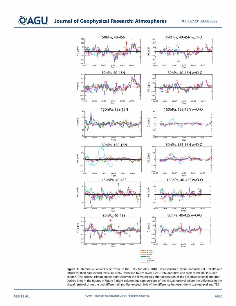
Figure 7. Interannual variability of ozone in the UTLS for 2005–2010. Deseasonalized ozone anomalies at 150 hPa and80 hPa for (first and second rows) 40–45°N, (third and fourth rows) 15°S–15°N, and (fifth and sixth rows) 40–45°S. (leftcolumn) The original climatologies; (right column) the climatologies after application of the TES observational operator.Dashed lines in the figures in Figure 7 (right column) indicate portions of the virtual retrieval where the difference in thevirtual retrieval using the two different fill profiles exceeds 50% of the difference between the virtual retrieval and TES.



4. Discussion

While the use of zonal mean climatologiesfor detailed UTLS process studies isobviously limited, the SPARCData Initiativeclimatologies nevertheless represent ourbest knowledge of the abundance andtemporal variability of ozone in the UTLS,and the characterization of the data setspresented here will provide valuableinformation for model evaluation. Forexample, a recent paper examinedclimatological differences in ozonebetween the suite of AtmosphericChemistry and Climate ModelIntercomparison Project (ACCMIP)models and TES and found that largebiases in the models’ UTLS ozone relativeto TES correspond to biases in ozone’seffect on outgoing longwave radiation(OLR) exceeding 10mW/m2 [Bowmanet al., 2013]. However, the biases anduncertainties of the TES measurementswere not considered in the study. Figure 8shows the range of differences in annualmean zonal mean ozone between themodels and TES as a function of latitudeat 100hPa. The TES observational operatorhas not been applied to the modelsbecause it was not used in the originalanalysis. The models differ from TES byup to a factor of 2 in either direction

(differences between the stratosphere-focused Chemistry-Climate Model Validation 2 (CCMVal-2) projectmodels and observations were similar in magnitude in the tropics and ~10% smaller in the extratropics [SPARCCCMVal, 2010]). The relative differences between the original satellite climatologies, as well as the ozonesondeclimatology, and TES are also shown and are much smaller than the model-TES differences at all latitudes.The measurements thus provide meaningful constraints for the models. The black dashed lines represent a“best estimate range” for ozone (defined by including a preponderance of the measurements) based onthe measurement climatologies and could be used to quantitatively evaluate the models with a robustcharacterization of the uncertainty in our knowledge of the ozone abundances. We note that theuncertainty range could be further reduced by accounting for differences in vertical resolution betweenthe climatologies (applying the TES observational operator to both the satellite and ozonsonde climatologies)and accounting for the sparse sampling of the ozonesonde climatology. The range of model differencesfrom TES would likewise be reduced by applying the observational operator but would still be much largerthan the measurement range.

The characterization of the SPARC Data Initiative climatologies presented here can also be used to providerobust quantification of the seasonal cycle in ozone in the UTLS, which has been used to evaluate modelrepresentation of transport and photochemistry [e.g., SPARC CCMVal, 2010; Gettelman et al., 2010; Hegglinet al., 2010]. The seasonal cycle of ozone near the tropical tropopause (~100 hPa) is determined by chemicalproduction, vertical transport, and mixing in of extratropical air, and the amplitude and phase reflectvariations in the relative contributions of these processes. While the climatologies differ in amplitude by upto 85% at 100 hPa in the tropics, the peak-to-peak amplitude of the seasonal cycle in the CCMVal-2 modelsvaried by a factor of >5 at 100 hPa in the same region, and two of the models misrepresented the phaseby> 4months [SPARC CCMVal, 2010; Gettelman et al., 2010]. In the extratropical lowermost stratosphere,

-50 0 50Latitude

-100

-50

0

50

100

Figure 8. Meridional profile of differences between ACCMIP models/SPARC Data Initiative climatologies and TES for 2005–2010. Grey shadedregion shows the range of relative differences in 100 hPa annual meanzonal mean ozone between the ACCMIP models and TES ((Model� TES)/TES) from Bowman et al. [2013]. The TES observational operator has notbeen applied to the model output because it was not used in the originalstudy. Colored lines show the differences between the SPARC DataInitiative climatologies and TES, and black circles represent the ozone-sonde climatology relative difference from TES. Black dashed lines showthe range of ozone consistent with a preponderance of the observationalclimatologies at each latitude.



the seasonal cycle has been used to evaluate the balance between the large-scale stratospheric circulation,which carries photochemically aged air downward into the region [Logan, 1999], and the breaking ofsynoptic-scale waves above the subtropical jet that brings in “young” tropical air masses [e.g., SPARC CCMVal,2010; Hegglin et al., 2010]. These processes together act to determine the distribution of radiatively activespecies in the UTLS.

The CCMVal-2 models reproduce the 100hPa seasonal cycle in midlatitudes much more consistently than inthe tropics but still vary in peak-to-peak amplitude by almost a factor of 2, while the measurements agree towithin 15% (with the exception of TES in the southern midlatitudes). This analysis provides a well-characterizeddata set for quantitative evaluation of model representation of the ozone seasonal cycle, as well as El Niño–Southern Oscillation/QBO variability in midlatitude ozone (section 3.6), for future studies.

5. Summary and Conclusions

We have presented the first comprehensive intercomparison of the currently available satellite climatologiesin the UTLS region. Comparing climatologies from instruments with different viewing geometries, samplingpatterns, and vertical resolution requires methodologies that account for these differences, particularly inregions with strong trace gas gradients such as the UTLS. To compare the monthly mean, zonal meanozone climatologies from the SPARC Data Initiative, we used the TES observational operator to verticallysmooth the climatologies from the higher-resolution limb-viewing instruments. This approach provides acommon basis for comparison of the large-scale ozone morphology as well as the seasonal and interannualvariability of ozone within the UTLS. However, our approach has several limitations, including the fact thatthe virtual retrievals can be sensitive to how one chooses to “fill in” the profiles below lowest measurementlevel of the limb sounders, that the TES sensitivity varies in the UTLS such that the a priori profile has asignificant influence near 150hPa in the extratropics, and that the averaging kernels are not fully independentof the ozone abundance, resulting in errors in the virtual retrievals that are difficult to quantify. We have triedto account for these factors when possible and to focus on robust differences in the UTLS climatologies.

The TES observational operator smoothes small-scale ozone structures and due to the influence of the a prioritends to increase tropical-extratropical ozone gradients as well as midlatitude vertical ozone gradients in theclimatologies from the limb-viewing instruments. It also reduces and vertically smoothes the differencesbetween the limb climatologies and TES. The TES observational operator reduces the temporal variability ofthe ozone climatologies from the high-resolution instruments but also greatly improves the consistencybetween them. This indicates that the differences in vertical resolution among the limb-viewing instrumentsmake a substantial contribution to differences in their retrieved ozone distributions both relative to TES andrelative to one other.

Most of the limb-viewing instruments have climatological mean positive differences (ranging from 5 to 75%)relative to TES ozone in the tropics, though for several instruments the differences depend strongly on thefill profile below ~100 hPa. For p≤ 100 hPa, the positive difference from TES likely reflect true positive biasesfor the climatologies given TES’s lack of bias with respect to the ozonsonde climatology. In the NorthernHemisphere extratropics, only the HIRDLS and MIPAS climatologies have differences with respect to TESthat are >15% and are also independent of the fill profile (Figure 4). In the southern extratropics, the TESobservational operator greatly reduces differences between the limb sounder climatologies and TES dueto TES’s low sensitivity at the pressure levels where the differences between the original climatologies andTES are largest.

There are large differences in the timing andmagnitude of the seasonal cycle in the tropical upper troposphere,though the amplitude differences are only ~1/3 those seen in models. At p≤ 100hPa, the climatologies showa more consistent tropical seasonal cycle, particularly when smoothed to the TES vertical resolution. The TESobservational operator reduces the differences in seasonal cycle amplitude to within 20% of TES for allinstruments except HIRDLS. In general, there is very good agreement among the climatologies regardingboth the timing and magnitude of the seasonal cycle in midlatitudes, except that ozone from the OSIRIS andSCIAMACHY climatologies is ~15% low relative to the other instruments during the southern midlatitudemaximum, likely due to their limited sampling of this region. All of the climatologies show low interannualvariability in the tropics (except for HIRDLS) and higher variability in midlatitudes, with northern midlatitudeinterannual variability greatly exceeding that in southern midlatitudes for p> 80hPa. The sampling of the



ACE-FTS instrument is insufficient to capture interannual variability on monthly time scales in the tropics.The TES observational operator greatly reduces the interannual variability in ozone from the limb sounderclimatologies for p> 100 hPa in the tropics and p> 200 hPa in midlatitudes. This improves the consistencybetween the data sets but may limit the usefulness of the virtual retrievals for quantifying UTLS variability.

This work represents an important first step in assessing the differences between satellite climatologies inthe UTLS region and provides a template for comparison of measurements from limb- and nadir-viewinginstruments. It also provides a well-characterized data set for model evaluation of zonal mean ozoneabundances and the seasonal and interannual variability of ozone. However, a much more detailed UTLSintercomparison using high spatial and temporal resolution measurements of multiple species is needed tofully characterize differences between instruments in this region and has been proposed as a follow on to theSPARC Data Initiative. It will require diagnostic tools that minimize geophysical variability and differencesin sampling and resolution such as tracer-tracer correlations, probability distribution functions, tropopause-relative vertical coordinates, and jet-based coordinates [e.g., Hegglin et al., 2008; SPARC CCMVal, 2010;Manneyet al., 2011]. Such an analysis promises to not only provide a detailed assessment of the quality of the satellitedata but also to improve our understanding of UTLS structure and processes.

ReferencesAghedo, A. M., K. W. Bowman, D. T. Shindell, and G. Faluvegi (2011), The impact of orbital sampling, monthly averaging and vertical resolution on

climate chemistry model evaluation with satellite observations, Atmos. Chem. Phys., 11(13), 6493–6514, doi:10.5194/acp-11-6493-2011.Beer, R. (2006), TES on the aura mission: Scientific objectives, measurements, and analysis overview, IEEE Trans. Geosci. Remote Sens., 44(5),

1102–1105, doi:10.1109/TGRS.2005.863716.Beer, R., T. A. Glavich, and D. M. Rider (2001), Tropospheric emission spectrometer for the Earth Observing System’s Aura satellite, Appl. Opt.,

40, 2356–2367, doi:10.1364/AO.40.002356.Bowman, K. W., T. Steck, H. M. Worden, J. Worden, S. Clough, and C. Rodgers (2002), Capturing time and vertical variability of tropospheric

ozone: A study using TES nadir retrievals, J. Geophys. Res., 107(D23), 4723, doi:10.1029/2002JD002150.Bowman, K. W., et al. (2006), Tropospheric Emission Spectrometer: Retrieval method and error analysis, IEEE Trans. Geosci. Remote Sens., 44(5),

1297–1307, doi:10.1109/TGRS.2006.871234.Bowman, K. W., et al. (2013), Evaluation of ACCMIP outgoing longwave radiation from tropospheric ozone using TES satellite observations,

Atmos. Chem. Phys., 13, 4057–4072, doi:10.5194/acp-13-4057-2013.Boxe, C. S., et al. (2010), Validation of northern latitude Tropospheric Emission Spectrometer stare ozone profiles with ARC-IONS sondes

during ARCTAS: Sensitivity, bias and error analysis, Atmos. Chem. Phys., 10, 9901–9914, doi:10.5194/acp-10-9901-2010.Degenstein, D. A., A. E. Bourassa, C. Z. Roth, and E. J. Llewellyn (2009), Limb scatter ozone retrieval from 10 to 60 km using a multiplicative

algebraic reconstruction technique, Atmos. Chem. Phys., 9(17), 6521–6529, doi:10.5194/acp-9-6521-2009.Dupuy, E., et al. (2009), Validation of ozone measurements from the Atmospheric Chemistry Experiment (ACE), Atmos. Chem. Phys., 9(2),

287–343, doi:10.5194/acp-9-287-2009.Folkins, I., P. Bernath, C. Boone, G. Lesins, N. Livesey, A. M. Thompson, K. Walker, and J. C. Witte (2006), Seasonal cycles of O3, CO, and con-

vective outflow at the tropical tropopause, Geophys. Res. Lett., 33, L16802, doi:10.1029/2006GL026602.Forster, P. M., and K. P. Shine (2002), Assessing the climate impacts of trends in stratospheric water vapour, Geophys. Res. Lett., 29, 1086–1089,

doi:10.1029/2001GL013909.Froidevaux, L., et al. (2008), Validation of Aura Microwave Limb Sounder stratospheric ozone measurements, J. Geophys. Res., 113, D15S20,

doi:10.1029/2007JD008771.Funke, B., and T. von Clarmann (2012), How to average logarithmic retrievals?, Atmos. Meas. Tech., 5(4), 831–841, doi:10.5194/amt-5-831-2012.Gettelman, A., et al. (2010), Multimodel assessment of the upper troposphere and lower stratosphere: Tropics and global trends, J. Geophys.

Res., 115, D00M08, doi:10.1029/2009JD013638.Gettelman, A., P. Hoor, L. L. Pan, W. J. Randel, M. I. Hegglin, and T. Birner (2011), The extra tropical upper troposphere and lower stratosphere,

Rev. Geophys., 49, RG3003, doi:10.1029/2011RG000355.Gille, J., et al. (2008), High Resolution Dynamics Limb Sounder: Experiment overview, recovery, and validation of initial temperature data,

J. Geophys. Res., 113, D16S43, doi:10.1029/2007JD008824.Hegglin, M. I., C. D. Boone, G. L. Manney, T. G. Shepherd, K. A. Walker, P. F. Bernath, W. H. Daffer, P. Hoor, and C. Schiller (2008), Validation of

ACE-FTS satellite data in the upper troposphere/lower stratosphere (UTLS) using non-coincident measurements, Atmos. Chem. Phys., 8,1483–1499, doi:10.5194/acp-8-1483-2008.

Hegglin, M. I., C. D. Boone, G. L. Manney, and K. A. Walker (2009), A global view of the extratropical tropopause transition layer from AtmosphericChemistry Experiment Fourier transform spectrometer O3, H2O, and CO, J. Geophys. Res., 114, D00B11, doi:10.1029/2008JD009984.

Hegglin, M. I., et al. (2010), Multi-model assessment of the upper troposphere and lower stratosphere: Extra-tropics, J. Geophys. Res., 115,D00M09, doi:10.1029/2010JD013884.

Jiang, Y. B., et al. (2007), Validation of Aura Microwave Limb Sounder ozone by ozonesonde and lidar measurements, J. Geophys. Res., 112,D24S34, doi:10.1029/2007JD008776.

Jones, D. B. A., K. W. Bowman, J. A. Logan, C. L. Heald, J. Liu, M. Luo, J. Worden, and J. Drummond (2009), The zonal structure of tropical O3 andCO as observed by the Tropospheric Emission Spectrometer in November 2004. Part I. Inverse modeling of CO emissions, Atmos. Chem.Phys., 9, 3547–3562, doi:10.5194/acp-9-3547-2009.

Konopka, P., J. U. Grooß, G. Günther, F. Ploeger, R. Pommrich, R. Müller, and N. Livesey (2010), Annual cycle of ozone at and above the tropicaltropopause: Observations versus simulations with the Chemical Lagrangian Model of the Stratosphere (CLaMS), Atmos. Chem. Phys., 10,121–132, doi:10.5194/acp-10-121-2010.

Kulawik, S. S., et al. (2006), TES atmospheric profile retrieval characterization: An orbit of simulated observations, IEEE Trans. Geosci. RemoteSens., 44(5), 1324–1332, doi:10.1109/TGRS.2006.871207.

AcknowledgmentsThe authors thank the relevant instru-ment teams and space agencies fortheir data and support. We also thankthe ISSI in Bern for facilitating two suc-cessful team meetings in Bern as part ofthe ISSI International Team activity pro-gram, and the SPARC Toronto office andSPARC/WCRP for travel support. Work atthe Jet Propulsion Laboratory, CaliforniaInstitute of Technology, was performedunder contract from the NationalAeronautics and Space Administration.John Gille and the work of the HIRDLSteam in the U.S. was supported by NASAcontract NAS5-97046. Michaela IHegglin’s work within the SPARC DataInitiative was supported by the CSA andESA. IAA was supported by the SpanishMINECO under grant AYA2011-23552and EC FEDER funds. The work of theUniversity of Bremen team on theSCIAMACHY ozone climatology wasfunded in part by the GermanAerospace Agency (DLR) within theproject SADOS (50EE1105) and by thestate and University of Bremen. ACE is aCanadian-led mission mainly supportedby the Canadian Space Agency (CSA).Development of the ACE-FTS climatolo-gies was supported by grants from theCanadian Foundation for Climate andAtmospheric Sciences and the CSA. Theozonesonde climatology and ACCMIPmodel results were provided by PaulYoung of Lancaster University and KevinBowman of the Jet PropulsionLaboratory, respectively.



http://dx.doi.org/10.5194/acp&hyphen;11&hyphen;6493&hyphen;2011

http://dx.doi.org/10.1109/TGRS.2005.863716

http://dx.doi.org/10.1364/AO.40.002356

http://dx.doi.org/10.1029/2002JD002150






http://dx.doi.org/10.1029/2006GL026602

http://dx.doi.org/10.1029/2001GL013909

http://dx.doi.org/10.1029/2007JD008771

http://dx.doi.org/10.5194/amt&hyphen;5&hyphen;831&hyphen;2012

http://dx.doi.org/10.1029/2009JD013638

http://dx.doi.org/10.1029/2011RG000355

http://dx.doi.org/10.1029/2007JD008824


http://dx.doi.org/10.1029/2008JD009984

http://dx.doi.org/10.1029/2010JD013884

http://dx.doi.org/10.1029/2007JD008776




Logan, J. A. (1999), An analysis of ozonesonde data for the troposphere: Recommendations for testing 3-D models, and development of agridded climatology for tropospheric ozone, J. Geophys. Res., 104, 16,115–16,149, doi:10.1029/1998JD100096.

Manney, G. L., et al. (2011), Jet characterization in the upper troposphere/lower stratosphere (UTLS): Applications to climatology andtransport studies, Atmos. Chem. Phys., 11, 6115–6137, doi:10.5194/acp-11-6115-2011.

Mieruch, S., et al. (2012), Global and long-term comparison of SCIAMACHY limb ozone profiles with correlative satellite data (2002–2008),Atmos. Meas. Tech., 5(4), 771–788, doi:10.5194/amt-5-771-2012.

Nardi, B., et al. (2008), Initial validation of ozone measurements from the High Resolution Dynamics Limb Sounder, J. Geophys. Res., 113,D16S36, doi:10.1029/2007JD008837.

Nassar, R., et al. (2008), Validation of Tropospheric Emission Spectrometer (TES) nadir ozone profiles using ozonesonde measurements,J. Geophys. Res., 113, D15S17, doi:10.1029/2007JD008819.

Neu, J. L., T. Flury, G. L. Manney, M. L. Santee, N. J. Livesey, and J. Worden (2014), Tropospheric ozone variations governed by changes instratospheric circulation, Nature Geosci., 7, 340–344, doi:10.1038/ngeo2138.

Peevey, T. R., J. C. Gille, C. E. Randall, and A. Kunz (2012), Investigation of double tropopause spatial and temporal global variability utilizingHigh Resolution Dynamics Limb Sounder temperature observations, J. Geophys. Res., 117(D01), 105, doi:10.1029/2011JD016443.

Ploeger, F., P. Konopka, R. Müller, S. Fueglistaler, T. Schmidt, J. C. Manners, J.-U. Grooß, G. Günther, P. M. Forster, andM. Riese (2012), Horizontaltransport affecting trace gas seasonality in the Tropical Tropopause Layer (TTL), J. Geophys. Res., 117, D09303, doi:10.1029/2011JD017267.

Randel, W. J., M. Park, F. Wu, and N. Livesey (2007), A large annual cycle in ozone above the tropical tropopause linked to the Brewer-Dobsoncirculation, J. Atmos. Sci., 64, 4479–4488, doi:10.1175/2007JAS2409.1.

Rodgers, C. (2000), Inverse Methods for Atmospheric Sounding: Theory and Practice, World Scientific, London.Rodgers, C. D., and B. J. Connor (2003), Intercomparison of remote sounding instruments, J. Geophys. Res., 108(D3), 4116, doi:10.1029/2002JD002299.Solomon, S., et al. (Eds.) (2007), Contribution of Working Group I to the Fourth Assessment Report of the Intergovernmental Panel on Climate

Change, 2007, Cambridge Univ. Press, Cambridge.Stratosphere-troposphere Processes and their Role in Climate Chemistry-Climate Model Validation (SPARC CCMVal) (2010), SPARC CCMVal

report on the evaluation of Chemistry-Climate Models, SPARC Rep. 5, WCRP-132, WMO/TD-1526, edited by D. W. Waugh, V. Eyring,and T. G. Shepherd, Zurich, Switzerland.

Tegtmeier, S., et al. (2013), SPARC Data Initiative: A comparison of ozone climatologies from international satellite limb sounders, J. Geophys.Res. Atmos., 118, 12,229–12,247, doi:10.1002/2013JD019877.

Thompson, A. M., et al. (2003), Southern Hemisphere Additional Ozonesondes (SHADOZ) 1998–2000 tropical ozone climatology 1.Comparison with Total Ozone Mapping Spectrometer (TOMS) and ground-based measurements, J. Geophys. Res., 108(D2), 8238,doi:10.1029/2001JD000967.

Toohey, M., et al. (2013), Characterizing sampling biases in the trace gas climatologies of the SPARC Data Initiative, J. Geophys. Res. Atmos.,118, 11,847–11,862, doi:10.1002/jgrd.50874.

Verstraeten, W. W., K. F. Boersma, J. Zörner, M. A. F. Allaart, K. W. Bowman, and J. R. Worden (2013), Validation of six years of TES troposphericozone retrievals with ozonesonde measurements: Implications for spatial patterns and temporal stability in the bias, Atmos. Meas. Tech., 6,1413–1423, doi:10.5194/amt-6-1413-2013.

von Clarmann, T., et al. (2009), Retrieval of temperature, H2O, O3, HNO3, CH4, N2O, ClONO2 and ClO fromMIPAS reduced resolution nominalmode limb emission measurements, Atmos. Meas. Tech., 2(1), 159–175, doi:10.5194/amt-2-159-2009.

Worden, H. M., et al. (2007), Comparisons of Tropospheric Emission Spectrometer (TES) ozone profiles to ozonesondes: Methods and initialresults, J. Geophys. Res., 112, D03309, doi:10.1029/2006JD007258.

Worden, H. M., K. W. Bowman, J. R. Worden, A. Eldering, and R. Beer (2008), Satellite measurements of the clear-sky greenhouse effect fromtropospheric ozone, Nat. Geosci., 1, 305–308, doi:10.1038/ngeo182.

Worden, H.M., K.W. Bowman, S. S. Kulawik, andA.M. Aghedo (2011), Sensitivity of outgoing longwave radiative flux to the global vertical distributionof ozone characterized by instantaneous radiative kernels from Aura TES, J. Geophys. Res., 116, D14115, doi:10.1029/2010JD015101.

Worden, J. S., S. S. Kulawik, M. Shepard, S. Clough, H. Worden, K. Bowman, and A. Goldman (2004), Predicted errors of Tropospheric EmissionSpectrometer nadir retrievals from spectral window selection, J. Geophys. Res., 109, D09308, doi:10.1029/2004JD004522.

World Meteorological Organization (2011), Scientific Assessment of Ozone Depletion: 2010, Global Ozone Research and Monitoring Project-Report 52, 516 pp., Geneva, Switzerland.



http://dx.doi.org/10.1029/1998JD100096



http://dx.doi.org/10.1029/2007JD008837

http://dx.doi.org/10.1029/2007JD008819

http://dx.doi.org/10.1038/ngeo2138

http://dx.doi.org/10.1029/2011JD016443

http://dx.doi.org/10.1029/2011JD017267

http://dx.doi.org/10.1175/2007JAS2409.1

http://dx.doi.org/10.1029/2002JD002299

http://dx.doi.org/10.1002/2013JD019877

http://dx.doi.org/10.1029/2001JD000967

http://dx.doi.org/10.1002/jgrd.50874



http://dx.doi.org/10.1029/2006JD007258

http://dx.doi.org/10.1038/ngeo182

http://dx.doi.org/10.1029/2010JD015101

http://dx.doi.org/10.1029/2004JD004522

the sparc data initiative: comparison of upper troposphere

Documents