A structure-preserving split finite element discretization of

the split 1D wave equations

Werner Bauer∗, Jorn Behrens†

Abstract

We introduce a new finite element (FE) discretization framework applicable for covariantsplit equations. The introduction of additional differential forms (DF) that form pairs with theoriginal ones permits the splitting of the equations into topological momentum and continuityequations and metric-dependent closure equations that apply the Hodge-star operator. Ourdiscretization framework conserves this geometrical structure and provides for all DFs properFE spaces such that the differential operators (here gradient and divergence) hold in strongform. We introduce lowest possible order discretizations of the split 1D wave equations,in which the discrete momentum and continuity equations follow by trivial projections ontopiecewise constant FE spaces, omitting partial integrations. Approximating the Hodge-star bynontrivial Galerkin projections (GP), the two discrete metric equations follow by projectionsonto either the piecewise constant (GP0) or piecewise linear (GP1) space.

Out of the four possible realizations, our framework gives us three schemes with significantlydifferent behavior. The split scheme using twice GP1 is unstable and shares the dispersion re-lation with the P1–P1 FE scheme that approximates both variables by piecewise linear spaces(P1). The split schemes that apply a mixture of GP1 and GP0 share the dispersion relationwith the stable P1–P0 FE scheme that applies piecewise linear and piecewise constant (P0)spaces. However, the split schemes exhibit second order convergence for both quantities ofinterest. For the split scheme applying twice GP0, we are not aware of a corresponding stan-dard formulation to compare with. Though it does not provide a satisfactory approximationof the dispersion relation as short waves are propagated much too fast, the discovery of thenew scheme illustrates the potential of our discretization framework as a toolbox to study andfind FE schemes by new combinations of FE spaces.

Keywords. Split linear wave equations, Split finite element method, Dispersion relation, Structure-preserving discretization, Shallow-water wave equation

2010 MSC. 76M10 (Primary), 65M60 (Secondary)

1 Introduction

The Finite Element (FE) method provides a powerful framework to discretize partial differentialequations (PDEs) and includes methods to prove the discrete models’ convergence, stability, andaccuracy properties (see e.g. [8, 20]). By offering flexibility in the choice of computational (unstruc-tured, h/p-adapted) meshes (cf. [6]) while providing an approximation of the continuous PDEswith the required order of accuracy, FE discretizations are nowadays appreciated in all researchareas that apply numerical modeling.

Discretizations using finite element methods provide one important advantage over other meth-ods: Starting from a variational formulation the discretization follows simply by substituting thecontinuous by discrete function spaces (Galerkin methods) while the differential operators remainunchanged. There exist a large variety of different suitable FE spaces to choose from. However,not all choices lead to well-behaving schemes. In particular mixed FE schemes suffer from this

∗Department of Mathematics, Imperial College London, London, United Kingdom; w.bauer@imperial.ac.uk†Department of Mathematics/CEN-Center for Earth System Research and Sustainability, Universitat Hamburg,

Hamburg, Germany

1

arX

iv:1

703.

0765

8v2

[m

ath.

NA

] 1

5 Ju

n 20

17

problem, where different variables of the PDE system are represented by different FE spaces. Insuch schemes, certain combinations of FE spaces lead to instabilities that exhibit spurious modes,rendering the solutions useless, in particular when studying nonlinear phenomena. A famous ex-ample for an unstable scheme is given by an approximation of both velocity and height fields ofthe 1D shallow-water equations by piecewise linear functions (cf. [23] and Sect. 3), where it is wellknown that equal order FE pairs are always unstable [10].

In order to avoid unsuitable choices, the Finite Element Exterior Calculus (FEEC) method[2, 3] provides means for choosing a suitable pair of FE spaces that is guaranteed to lead to astable mixed discretization. In particular, FEEC puts geometrical constraints on the FE spacessuch that geometric properties, like the Helmholtz decomposition of vector-fields, are preserved inthe discrete case. As a result, FEEC pairs of spaces always satisfy the inf-sup condition [1] whilecombinations of FE spaces that are not stable are ruled out. For the above mentioned 1D waveequations, approximating the velocity with piecewise linear and the height field with piecewiseconstant spaces satisfies the requirements of FEEC and gives indeed a stable scheme (cf. again[23] and Sect. 3).

Although providing a very general mathematical framework, naturally there are issues for whichFEEC yields no satisfying answers. Let us consider, for instance, problems in geophysical fluiddynamics (GFD), in which an additional Coriolis term in the equations considers effects caused bythe earth’s rotation [22]. For an atmosphere in rest, the Coriolis force that depends on the velocityand the gradient of the pressure (or height) are in geostrophic balance. To maintain this balancein the discretization, the pressure (or height) field should be represented discretely at one order ofconsistency higher than that of the velocity field. Unfortunately, this contradicts the requirementimposed by FEEC on this FE pair. In [10], this issue could be resolved by applying a combinationof FE and Discontinuous Galerkin (DG) spaces.

Moreover, in order to meet the regularity requirement of the chosen FE pairs, FEEC requiresthe PDEs to be written in weak variational form, in which partial integration has been performed.As pointed out recently in [15], the conventional mixed (weak) form of the equations causes cer-tain operators, such as the co-derivative, to be non-local (global) operators. As a consequence,such FEEC methods are not locally volume preserving, which reduces the quality of the localrepresentation of the quantities of interest (cf. [15]).

In this manuscript our main goal is to introduce a FE discretization framework that providesan alternative methodology to avoid mentioned unsuitable FE choices with GFD in mind. Morespecifically, we develop a framework that applies two FEEC pairs instead of one, therefore providinga larger variety of different combinations of FE spaces, in which both derivatives and co-derivativesare local operators. This framework is based on formulating the PDEs in split form, as introducedin [4, 5] for the GFD equations. The split equations consist of a topological and metric part whileemploying straight and twisted differential forms to adequately model the physical quantities ofinterest. The FE discretization framework translates this geometrical structure from the continuousto similarly structured discrete equations (cf. Sect. 2).

Our approach shares some basic ideas with other discretization techniques, in particular mimeticdiscretizations (see e.g. [9, 7, 13], and [21] for a historical overview). There, the PDEs are alsoformulated by differential forms and a clear distinction between purely topological and metricterms is achieved. Applying algebraic topology as discrete counterpart to differential geometry,the discrete equations mimic the underlying geometrical structure and are therefore denoted asstructure-preserving (cf. [14]). Similar ideas of distinguishing between metric-dependent andmetric-free terms in a GFD related context can also be found in [12] introducing FEEC discretiza-tions of the nonlinear rotating shallow-water equations. In spite of these similarities, none of theschemes associate a proper FE space to each variable, as suggested by our framework.

For the sake of a clear exposition, we focus on a simple example, the split 1D linear shallow-water set of equations. Extending our framework to treat also more practically relevant equations,such as the nonlinear rotating shallow-water equations, is subject of ongoing and future work. Byinvestigating structure-preserving methods that apply lowest order (piecewise linear and constant)FE spaces to keep computational costs low, we address the requirements of GFD in developingschemes that satisfy first principle conservation laws (i.e mass and momentum conservation) andthat are suited for simulations with integration times in the order of years and longer.

We structure the manuscript as follows. In Sect. 2, we introduce the split set of 1D wave

2

equations and motivate the use of the split form of equations as principle formulation for theirdiscretization. Recalling in Sect. 3 two low-order mixed FE schemes, namely the unstable P1–P1and the stable P1–P0 pairs, we introduce in Sect. 4 the new discretization framework, referred toas split FE method. We suggest a solving algorithm and present the schemes’ discrete dispersionrelations. Comparing them if possible with the conventional mixed schemes, we perform in Sect. 5numerical simulations to investigate conservation behavior, convergence rates, and accuracy of allschemes. Finally in Sect. 6, we draw conclusions and provide an outlook for ongoing and futurework.

2 Hierarchical structuring of the wave equation

In order to convey the basic ideas to the reader most clearly and comprehensively, we developour FE discretization framework on a simple example, the set of 1D wave equations. As the splitform of the equations (cf. [5]) is an essential ingredient of our approach, we first introduce thecorresponding split 1D wave equations and compare them with conventional formulations.

A hierarchical structuring of the wave equation. Compared to conventional formulations,the split 1D wave equations arrange themselves in the following hierarchy of linear wave equations:

1. one 2nd-order equation:∂2h(x, t)

∂t2− c2 ∂

2h(x, t)

∂x2= 0, (1)

with phase velocity c = ω/k for wave frequency ω and wave number k and with boundarycondition (BC) h(0, t) = h(L, t)∀t;

2. two 1st-order equations:

∂u(x, t)

∂t+ g

∂h(x, t)

∂x= 0,

∂h(x, t)

∂t+H

∂u(x, t)

∂x= 0, (2)

with phase velocity c =√gH and BCs h(0, t) = h(L, t), u(0, t) = u(L, t)∀t;

3. two 1st-order equations and two closure equations:

∂u(1)

∂t+ gdh(0) = 0,

∂h(1)

∂t+Hdu(0) = 0,

u(0) = ?u(1), h(1) = ?h(0),

(3)

with phase velocity c =√gH and BCs h(0)(0, t) = h(0)(L, t), u(0)(0, t) = u(0)(L, t)∀t;

for a periodic domain x ∈ [0, L]. The smooth function h(x, t) denotes the height elevation withmean fluid height H while assuming a trivial bottom topography. The smooth function u(x, t) de-notes the velocity of some fluid parcel in direction of x at time t ∈ [0, T ] ⊂ R. g is the gravitationalacceleration. Describing the momentum and height of a shallow water column, equations (2) areusually referred to as shallow-water equations. Throughout this manuscript however, we will referto the preceding formulations as wave equations.

The splitting of equations (3) into topological (first line) and metric parts (second line) isbased on their formulation in terms of differential forms: u(1) ∈ (Λ1; 0, T ) denotes a time-dependentstraight 1-form and h(0) ∈ (Λ0; 0, T ) a time-dependent straight 0-form (straight function) – straight

forms do not change their signs when the orientation of the manifold changes; u(0) ∈ (Λ0; 0, T )

denotes a time-dependent twisted 0-form and h(1) ∈ (Λ1; 0, T ) a time-dependent twisted 1-form –twisted forms compensate the change in signs which would result from a change in orientation. Thelatter property is shared by the twisted Hodge-star operator ? : Λk → Λ(1−k) (resp. Λk → Λ(1−k))mapping from straight (resp. twisted) k-forms to twisted (resp. straight) (1 − k)-forms, here for

k = 0, 1, as we are in one dimension. The index (k) denotes the degree, and Λk, Λk the space of allk-forms.

3

The exterior derivative is defined as the map d : Λ0 → Λ1 (or d : Λ0 → Λ1 for twisted forms,cf. diagram (25)). It reduces in one dimension to the total derivative of a smooth function f(x),i.e. for f (0) ∈ Λ0,df (0) = ∂xf(x)dx ∈ Λ1. The map of d on twisted forms is defined analogously.

We refer the reader to Sec. 4.1 for an explicit representation of the split wave equations (3) inthe local coordinate x ∈ [0, L], and to [5] for an elaborated discussion about straight and twistedforms, the twisted Hodge-star operators, and the derivation of n-dimensional split equations ofGFD.

The split wave equations: We argued in detail in [5] why it is favorable to represent theequations of GFD in terms of differential forms rather than vector-calculus notation, and wediscussed advantages of the split form in particular. Here, the split representation of the waveequations fits naturally into the arrangement of wave equations presented above, in which thesaddle point (mixed) form (2) results from a splitting of the standard form (1), and the splitform (3) from a further splitting of the saddle point form (2). This somehow suggests to study inmore detail possible benefits of a discretization based on the split form (3) rather than on the mixedform (2), just as there exist cases in which discretizations based on equations (2), usually discretizedby mixed FE methods, perform better than schemes resulting from standard FE approaches thatrely on formulation (1).

Let us first elaborate on the latter point, for which we present two examples where standardFE schemes even fail to provide correct solutions. As pointed out in [3], the standard FE solutionto the vector Poisson equation on non-convex polyhedral domains will converge to a false solutionof the problem for almost all forcing functions f . The same happens when calculating standard FEsolutions for the vector Laplacian on an annulus. However, correct solutions can be obtained whenusing mixed formulations, in particular those based on FEEC [3]. In addition, mixed formulations,in which two or even more FE spaces are used to approximate separate variables, are well suitedfor saddle point problems. These arise, for instance, in constrained minimization problems (Stokesequations or Darcy flow), in which the elimination of one of the variables is not possible (cf. [20],Chapter 36). In this latter case, equations in form (1) do even not exist. There are also somephysical and numerical reasons in favor of mixed FE methods. According to [18], it is the first-order system, such as (2), that follows from physics (i.e. from first conservation principles of massand momentum) and not the second-order equation, such as (1). In particular, efficient numericalschemes can be derived more easily from the first-order system.

Following in particular the latter line of argumentation, the split form more accurately modelsthe physical properties than the first-order system, because system (3) provides for each variablethe adequate (straight or twisted) differential form that suits in dimension and orientation thecorresponding property of a real fluid (cf. [5], Section 7). It seems appropriate during the dis-cretization process to provide for each variable a suitable FE space too. As a proof of concept, oneaim of this manuscript is to exploit this additional freedom in the choice of FE spaces and study,in terms of convergence, accuracy, stability and dispersion relation, possible advantages, but alsodrawbacks, that come along with this generalized FE method.

More precisely, by using the split form of the equations, we approximate each variable by a FEspace such that the discrete version of the exterior derivative d satisfies the mappings Λ0

h → Λ1h

and Λ0h → Λ1

h. Λih, Λih, i = 0, 1, are FE spaces that approximate the corresponding continuous

spaces. As pointed out later in more detail, this approach guarantees correct discrete topologicalequations up to projection error caused by projecting the continuous equations into the FE spaces.Any additional errors are caused by the metric-dependent closure equations that are realized bynontrivial projections between straight and twisted spaces (cf. Sect. 4). Such a clear separationbetween projection and additional errors, the latter caused by partial integrations in the weakform, is not obvious in mixed FE methods. Part of future work will be to study how these differenterror sources relate.

3 The mixed finite element method

In this section, we briefly review two examples of the general idea behind mixed FE methods andwe introduce notations and definitions required for the remainder of the paper. First, we observe

4

xl=1 = 0 xN+1 = Lxlxl−1 xl+1xm−1 xm

l = 1m = 1

ll − 1 l + 1 l = N

m− 1 m m = Nm+ 1

xm+1

χm+1(x)φl(x)

b

b

b

b

b

b

b

b

b

b

b

b

b b b b b b

bb

b b b

Figure 1: Discretization of the periodic domain x ∈ [0, L] by N subintervals (elements) and Nindependent nodes; the former are denoted by m, the latter by l for m, l = 1, .., N . φl(x) are thebasis functions of V 1

h and χm(x) of V 0h (cf. Appendix A for their definition).

that there are two equations for two prognostic variables in equation (2). In order to discretizethem one has the choice of mixing the corresponding FE spaces, which gives rise to the namingconvention. Here we consider (i) similar (V 1

h , V1h , ) or (ii) mixed FE spaces (V 1

h , V0h ), where V 1

h

refers to a linear and V 0h to a constant FE space.

In more detail, we subdivide the domain [0, L] into N subintervals [xl, xl+1], for l = 1, . . . N,as shown in Figure 1. We denote the points xl as nodes l and the subintervals as elements mwith centers xm := 1

2 (xl + xl+1) and element sizes ∆xm = (xl+1 − xl), for l,m = 1, . . . N . Basisfunctions and coefficients at nodes carry the subindices l and l′ and those at element centers thesubindices m and m′. To impose periodic boundary conditions, we identify the nodes at x = 0 andat x = L with each other and consider only 1 Degree of Freedom (DoF) associated to this node.We have thus N independent DoF for both nodes and elements.

Throughout this manuscript we will use the Lagrange functions {φl(x)}Nl=1 as basis for thepiecewise linear FE space V 1

h and the step functions {χm(x)}Nm=1 as basis for the piecewise constantFE space V 0

h (cf. Appendix A for their definitions).

3.1 The unstable P1–P1 finite element discretization

In order to find approximate solutions of the wave equations (2), we apply Galerkin’s method.To this end, we formulate the wave equations in variational form and approximate u(x, t) andh(x, t) by suitable discrete functions. Being aware of the problems of spurious modes (discussedbelow), we start with a naive choice of a pair of FE spaces approximating both u(x, t) and h(x, t)by piecewise linear (P1) functions uh(x, t) ∈ (V 1

h ; 0, T ) and hh(x, t) ∈ (V 1h ; 0, T ). We refer to this

scheme as P1–P1 scheme.The discrete variational form of the wave equations is then given by: find (uh(x, t), hh(x, t)) ∈

(V 1h ; 0, T )× (V 1

h ; 0, T ), such that∫L

(∂uh(x, t)

∂t+ g

∂hh(x, t)

∂x

)φ(x)dx = 0, ∀φ(x) ∈ V 1

h ⊂ V 1,∫L

(∂hh(x, t)

∂t+H

∂uh(x, t)

∂x

)φ(x)dx = 0, ∀φ(x) ∈ V 1

h ⊂ V 1,

(4)

for any test function φ(x) in the test space V 1h . Expanding the variables in terms of the basis of

the trial space V 1h ,

uh(x, t) ≈N∑l=1

ul(t)φl(x) and hh(x, t) ≈N∑l=1

hl(t)φl(x) , (5)

with time dependent coefficients ul(t) and hl(t), and varying the test functions φ(x) over the basis

5

functions {φl′(x)}Nl′=1 of the test space V 1h , we obtain

N∑l=1

∂tul(t)

∫L

φl(x)φl′(x)dx+ g

N∑l=1

hl(t)

∫L

dφl(x)

dxφl′(x)dx = 0, for l′ = 1, . . . , N,

N∑l=1

∂thl(t)

∫L

φl(x)φl′(x)dx+H

N∑l=1

ul(t)

∫L

dφl(x)

dxφl′(x)dx = 0, for l′ = 1, . . . , N.

(6)

This discrete system can analogously be written in matrix-vector formulation. Defining the co-efficient vectors un = (u1(t), ..., ul(t), ..., uN (t)) and hn = (h1(t), ..., hl(t), ..., hN (t)), with subindexn for nodes, we obtain the following linear system of algebraic equations:

Mnn ∂un∂t

+ gDnnhn = 0, Mnn ∂hn∂t

+HDnnun = 0, (7)

in which Mnn is a (N ×N) mass-matrix with metric-dependent coefficient

Mll′ =

∫L

φl(x)φl′(x)dx, (8)

and Dnn a (N ×N) stiffness-matrix with metric-independent coefficients

Dll′ =

∫L

dφl(x)

dxφl′(x)dx . (9)

In Appendix A, we provide explicit representations of these matrices for the mesh of Figure 1subject to periodic boundary conditions.

Time discretization. To discretize the semi-discrete equations (7) in time, we use the Crank-Nicolson (CN) scheme, a symmetric, implicit time discretization method. Then, for the timet ∈ [0, T ] and a time step size of ∆t, the full discretized matrix-vector equations read

Mnnunt+1 = Mnnun

t +1

2∆tgDnnhn

t +1

2∆tgDnnhn

t+1, (10)

Mnnhnt+1 = Mnnhn

t +1

2∆tHDnnun

t +1

2∆tHDnnun

t+1. (11)

We will solve these equations by fixed point iteration, even though they could be solved directly dueto the linearity. The motivation for this inefficient algorithmic choice lies in future work on non-linear equations and the possibility to treat possible kernels for the discrete Hodge-star operatorsin the split schemes (cf. (43)). For more details on the solver, we refer to Sect. 4.3 in which weintroduce a corresponding algorithm for the split finite element schemes.

The choice of using an iterative algorithm does not alter the results discussed in this paper.Only the time step size has to be restricted, in spite of the unconditional stability of the CN scheme.Similarly to the CFL number in explicit schemes, ∆t must not exceed a certain threshold µ in orderto guarantee that even the fastest waves are sufficiently well resolved and that the iterative solverconverges. Defining the CFL number for the 1D wave equations by

µ =√gH

∆t

∆x, (12)

we restrict ∆t for a given ∆x such that µ is smaller that some constant. This constant, determinedempirically for all test cases and mesh resolutions applied in this manuscript, is given for theunstable scheme by µ ≤ 1.15 (see Sect. 4.3 for more details).

Discussion about spatial stability. Throughout this paper, we study the stability propertiesof each discrete scheme by investigating whether it supports spurious modes. Such spurious modesare free modes, i.e. unphysical, very oscillatory small-scale waves on the grid scale that are notconstrained by the discrete equations. In case of nonlinear equations, these modes get coupled

6

to the smooth solution and grow fast, making the scheme unusable. Besides studying the inf-supcondition (see, e.g. [8]), one way of investigating the occurrence of such spurious modes is todetermine the dispersion relation of the discrete scheme.

For the unstable P1–P1 FE scheme, we associate spurious modes with those modes that showzero group velocity ω, for some wave numbers k. These modes are trapped to the grid scale andmay lead to the just described instabilities. More precisely, the angular frequency ω = ω(k) satisfiesthe dispersion relation (see Appendix B)

cd =ω

k= ±

√gH

sin(k∆x)

k∆x

[3

2 + cos(k∆x)

]. (13)

For small k → 0, the discrete dispersion relation converges to the continuous one with cd → c =√gH. However, besides the correct zero frequency at k = 0, this dispersion relation has at the

shortest wave length k = π∆x a second zero solution (spurious mode) with zero wave speed leading

to an unphysical standing wave.

3.2 The stable P1–P0 finite element discretization

The instability demonstrated in the previous subsection, caused by a choice of similar FE spacesfor both variables, is a general feature of methods with same FE spaces for approximating u and h(cf. [11]). To avoid this problem, we present a stable mixed FE method using different FE spacesto approximate velocity and height.

As proposed by other authors (e.g. [16]), we approximate u(x, t) by the piecewise linear (P1)function uh(x, t) ∈ (V 1

h ; 0, T ) and h(x, t) by the piecewise constant (P0) function hh(x, t) ∈(V 0h ; 0, T ) and we apply Galerkin’s method to find these approximations. We refer to this scheme

as P1–P0 scheme.The formulation of the wave equations (2) in variational form implies multiplication of the

momentum equation by a test function φ(x) ∈ V 1h and of the continuity equation by a test function

χ(x) ∈ V 0h . Because the derivative of hh(x, t) is not well-defined globally, the corresponding term

in the momentum equation requires integration by parts, whereas for the remaining terms trivialprojections into the corresponding spaces are suitable.

The discrete variational/weak form of the wave equations is thus given by: find (uh(x, t), hh(x, t)) ∈(V 1h ; 0, T )× (V 0

h ; 0, T ), such that∫L

(∂uh(x, t)

∂tφ(x)− ghh(x, t)

∂φ(x)

∂x

)dx = 0, ∀φ(x) ∈ V 1

h ⊂ V 1,∫L

(∂hh(x, t)

∂t+H

∂uh(x, t)

∂x

)χ(x)dx = 0, ∀χ(x) ∈ V 0

h ⊂ V 0.

(14)

The momentum equation is given in weak form, due to the integration by parts, while the continuityequations remains in variational form. The boundary terms from integration by parts in the weakmomentum equation vanish because of the periodic boundary conditions and continuity conditionsat cell interfaces. This special treatment is a source of additional error, while the trivially projectedterms do not introduce further errors beyond those caused by the approximation of the initialconditions by the FE spaces [11].

Expanding the variables in terms of the corresponding bases yields

uh(x, t) ≈N∑l=1

ul(t)φl(x) and hh(x, t) ≈N∑m=1

hm(t)χm(x). (15)

Substituting these expansions into equations (14) gives

N∑l=1

∂tul(t)

∫L

φl(x)φl′(x)dx− gN∑m=1

hm(t)

∫L

χm(x)dφl′(x)

dxdx = 0, for l′ = 1, . . . , N,

N∑m=1

∂thm(t)

∫L

χm(x)χm′(x)dx+H

N∑l=1

ul(t)

∫L

dφl(x)

dxχm′(x)dx = 0, for m′ = 1, . . . , N.

(16)

7

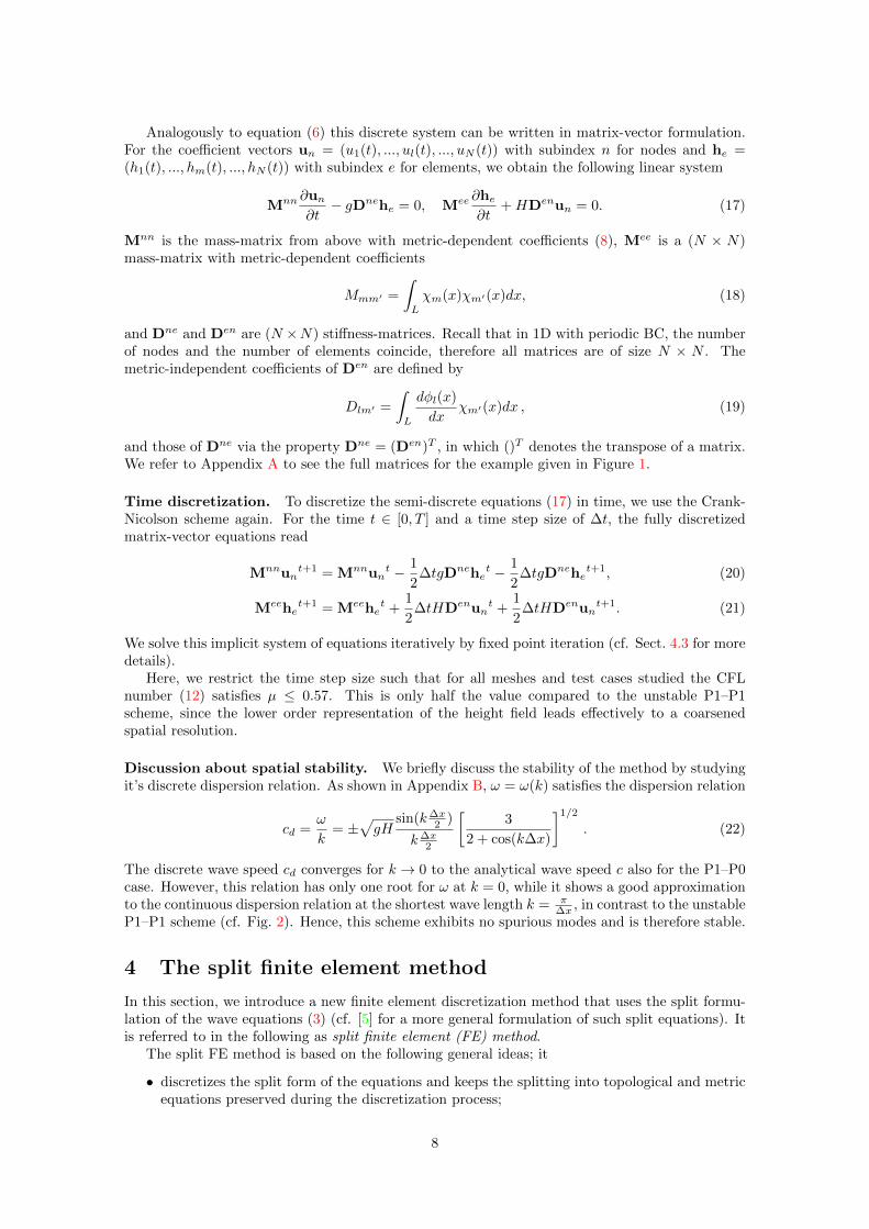
Analogously to equation (6) this discrete system can be written in matrix-vector formulation.For the coefficient vectors un = (u1(t), ..., ul(t), ..., uN (t)) with subindex n for nodes and he =(h1(t), ..., hm(t), ..., hN (t)) with subindex e for elements, we obtain the following linear system

Mnn ∂un∂t− gDnehe = 0, Mee ∂he

∂t+HDenun = 0. (17)

Mnn is the mass-matrix from above with metric-dependent coefficients (8), Mee is a (N × N)mass-matrix with metric-dependent coefficients

Mmm′ =

∫L

χm(x)χm′(x)dx, (18)

and Dne and Den are (N ×N) stiffness-matrices. Recall that in 1D with periodic BC, the numberof nodes and the number of elements coincide, therefore all matrices are of size N × N . Themetric-independent coefficients of Den are defined by

Dlm′ =

∫L

dφl(x)

dxχm′(x)dx , (19)

and those of Dne via the property Dne = (Den)T , in which ()T denotes the transpose of a matrix.We refer to Appendix A to see the full matrices for the example given in Figure 1.

Time discretization. To discretize the semi-discrete equations (17) in time, we use the Crank-Nicolson scheme again. For the time t ∈ [0, T ] and a time step size of ∆t, the fully discretizedmatrix-vector equations read

Mnnunt+1 = Mnnun

t − 1

2∆tgDnehe

t − 1

2∆tgDnehe

t+1, (20)

Meehet+1 = Meehe

t +1

2∆tHDenun

t +1

2∆tHDenun

t+1. (21)

We solve this implicit system of equations iteratively by fixed point iteration (cf. Sect. 4.3 for moredetails).

Here, we restrict the time step size such that for all meshes and test cases studied the CFLnumber (12) satisfies µ ≤ 0.57. This is only half the value compared to the unstable P1–P1scheme, since the lower order representation of the height field leads effectively to a coarsenedspatial resolution.

Discussion about spatial stability. We briefly discuss the stability of the method by studyingit’s discrete dispersion relation. As shown in Appendix B, ω = ω(k) satisfies the dispersion relation

cd =ω

k= ±

√gH

sin(k∆x2 )

k∆x2

[3

2 + cos(k∆x)

]1/2

. (22)

The discrete wave speed cd converges for k → 0 to the analytical wave speed c also for the P1–P0case. However, this relation has only one root for ω at k = 0, while it shows a good approximationto the continuous dispersion relation at the shortest wave length k = π

∆x , in contrast to the unstableP1–P1 scheme (cf. Fig. 2). Hence, this scheme exhibits no spurious modes and is therefore stable.

4 The split finite element method

In this section, we introduce a new finite element discretization method that uses the split formu-lation of the wave equations (3) (cf. [5] for a more general formulation of such split equations). Itis referred to in the following as split finite element (FE) method.

The split FE method is based on the following general ideas; it

• discretizes the split form of the equations and keeps the splitting into topological and metricequations preserved during the discretization process;

8

• treats straight and twisted variables independently and provides for each of them suitableFE spaces such that the topological momentum and continuity equations can be written invariational form without partial integration;

• provides FE spaces that form a pair of straight and twisted cohomology chains, in which dmaps between either straight or twisted chain elements according to diagram (25);

• represents the metric closure equations (Hodge-star operators) as projections between thestraight and twisted FE spaces (cf. diagram (25)).

Following these algorithmic ideas, the discretization of the topological equations is a trivial projec-tion into the corresponding FE spaces with only the projection error occurring. Additional errorsare introduced by metric-dependent closure equations, in which the discretization of the continuousHodge-star operators is performed by non-trivial projections between straight and twisted spaces.

4.1 Variational formulation of the split wave equation

Starting from the split wave equations (3), we seek a discretization by standard FE techniques.In particular, we want to apply Galerkin’s method, which implies to formulate the split waveequations in variational form.

Employing the notation of differential forms, we notice that the time-dependent differentialforms in (3) can be represented in the local coordinate x ∈ [0, L] with time parameter t ∈ [0, T ].Denoting with dx the dual basis to the tangential basis ∂x := ∂

∂x , the 1-forms are given by

u(1) = u(1)(x, t)dx ∈ (Λ1; 0, T ) and h(1) = h(1)(x, t)dx ∈ (Λ1; 0, T ). The 0-forms can be written

as h(0) = h(0)(x, t) ∈ (Λ0; 0, T ) and u(0) = u(0)(x, t) ∈ (Λ0; 0, T ). To distinguish the coordinatefunctions from the respective forms, the former carry the notation (x, t). The exterior derivative

d : Λ0 → Λ1 and d : Λ0 → Λ1 maps the corresponding 0-forms to the 1-forms dh(0)h = ∂xh

(0)h (x, t)dx

and du(0)h = ∂xu

(0)h (x, t)dx.

Furthermore, this coordinate representation allows us to describe the action of ? more precisely.It is defined via its action on the dual basis dx and the constant function 1 describing the unitvolume. In other words, denoting a choice of orientation as direct frame ’Or’ and it’s oppositeorientation as skew frame ’-Or’, then ? maps the straight 1-form dx ∈ Λ1 to the twisted 0-from ?dx = {1 in Or,−1 in -Or} ∈ Λ1 or the straight function 1 ∈ Λ1 to the twisted 1-form

?1 = {dx in Or,−dx in -Or} ∈ Λ1. For both the straight and the twisted Hodge-star operators aself-adjoint property holds (e.g. ?? = Id. cf. [5] for more details).

The idea behind the definition of twisted forms and the twisted Hodge-star is to guarantee thatthe equations remain the same in both direct and skew frames. To enhance readability, we willtherefore assume for the remainder of the manuscript to be in the direct frame ’Or’ in which ? mapsto the positive valued forms and skip an analogous derivation for the case of ’-Or’. However, wewill keep the notation˜ to distinguish between the various spaces. Using this local representation,the metric closure equations in (3) read:

u(0) = ?u(1) = u(1)(x, t)?dx = u(1)(x, t) and h(1) = ?h(0) = h(0)(x, t)?1 = h(0)(x, t)dx.

Split variational form of the split 1D wave equations. Using these local representations in(3) and multiplying the resulting equations by a test function χ(x) ∈ Λ1, we obtain the variational

form for the topological equations: find (u(1)(x, t), h(0)(x, t), h(1)(x, t), u(0)(x, t)) ∈ (Λ1; 0, T ) ×(Λ0; 0, T )× (Λ1; 0, T )× (Λ0; 0, T ) such that∫

L

(∂u(1)(x, t)

∂t+ g

∂h(0)(x, t)

∂x

)χ(x)dx = 0 , ∀χ(x) ∈ Λ1,∫

L

(∂h(1)(x, t)

∂t+H

∂u(0)(x, t)

∂x

)χ(x)dx = 0 , ∀χ(x) ∈ Λ1,

(23)

9

subject to the variational metric equations∫L

u(0)(x, t)τ i(x)dx =

∫L

u(1)(x, t)τ i(x)dx , ∀τ i(x) ∈ Λi, i = 0, 1,∫L

h(1)(x, t)τ j(x)dx =

∫L

h(0)(x, t)τ j(x)dx , ∀τ j(x) ∈ Λj , j = 0, 1.

(24)

The latter equations follow by multiplying the local representation of the metric equations in (3)with the test functions τ i,j(x), i, j = 0, 1, that can be elements of either Λ0 or Λ1.

Having four equations for four unknowns (the two straight and two twisted ones), the system isclosed. We will refer to this set of equations as split variational form of the split 1D wave equations.

4.2 Discrete split variational formulation

To discretize the split variational form (23) and (24) with Galerkin’s method, we approximate

the variables u(1), h(0), h(1), u(0) by suitable discrete k-forms u(1)h , h

(0)h , h

(1)h , u

(0)h , respectively. Fol-

lowing the above general ideas of the split FE method, the discrete k-forms with their straightand twisted FE spaces that approximate the corresponding continuous spaces should satisfy thefollowing diagram:

h(0)h ∈ Λ0

hd−−−−→ Λ1

h 3 u(1)h

?h1 /?h0

y y ?u1 /?u0h

(1)h ∈ Λ1

hd←−−−− Λ0

h 3 u(0)h

(25)

In the following we will provide definitions for these spaces and mappings.The preceding diagram is satisfied by the following set of FE spaces:

• Λ0h = V 1

h and Λ0h = V 1

h ;

• Λ1h = {ω(1)

h = ω(1)h (x)dx : ω

(1)h (x) ∈ V 0

h };

• Λ1h = {ω(1)

h = ω(1)h (x)dx : ω

(1)h (x) ∈ V 0

h };

with FE spaces V 1h and V 0

h from Sect. 3 with piecewise linear basis {φl(x)}Nl=1 and piecewiseconstant basis {χm(x)}Nm=1, respectively. Note that the superindices in V ih , i = 0, 1, correlate withthe polynomial degree whereas the superindices in Λih, i = 0, 1, denote the degree of the differentialforms. Choosing other, higher order FE spaces is also possible as long as the relationship betweenthese spaces satisfy diagram (25). For this manuscript however, we use the lowest order FE spacespossible. To establish time-dependent k-forms, we proceed as above for the mixed FE methods.

Approximating the continuous by discrete k-forms taken from the above FE spaces and sub-stituting into (23) and (24) give the discrete split variational form of the split 1D wave equations:

find (u(1)h (x, t), h

(0)h (x, t), h

(1)h (x, t), u

(0)h (x, t)) ∈ (Λ1

h; 0, T )× (Λ0h; 0, T )× (Λ1

h; 0, T )× (Λ0h; 0, T ) such

that ∫L

(∂u

(1)h (x, t)

∂t+ g

∂h(0)h (x, t)

∂x

)χ(x)dx = 0 , ∀χ(x) ∈ Λ1

h ⊂ Λ1,

∫L

(∂h

(1)h (x, t)

∂t+H

∂u(0)h (x, t)

∂x

)χ(x)dx = 0 , ∀χ(x) ∈ Λ1

h ⊂ Λ1,

(26)

for any test function χ(x) of the test space Λ1h ⊆ Λ1

h subject to the discrete variational metricequations

u(0)h = ?

u1−iu

(1)h by

∫L

u(0)h (x, t)τ i(x)dx =

∫L

u(1)h (x, t)τ i(x)dx , ∀τ i(x) ∈ Λih ⊂ Λi, i = 0, 1, (27)

h(1)h = ?

h1−jh

(0)h by

∫L

h(1)h (x, t)τ j(x)dx =

∫L

h(0)h (x, t)τ j(x)dx , ∀τ j(x) ∈ Λjh ⊂ Λj , j = 0, 1, (28)

10

for any test functions τ i,j(x) of the test spaces Λi,jh ⊆ Λi,jh . Equations (27) and (28) define the

discrete Hodge-star operators. We use the notation ?u1−i and ?

h1−j for i, j = 0, 1 to indicate that

?u1 /?

h1 project on piecewise linear (P1) and ?

u0 /?

h0 on piecewise constant (P0) spaces.

Equations (26) are trivial projections of the topological equations into the test space Λ1h of

piecewise constant test functions. The discrete exterior derivative d is a surjective map from piece-wise linear to piecewise constant functions and can be represented by the metric-free coincidencematrix Den (see below). The discrete topological equations are therefore exact up to the errorsthat occur by the projections into the piecewise constant spaces.

Equations (27) and (28) are nontrivial Galerkin projections between different spaces and pro-vide approximations of the Hodge-star operator. For solving the system, the discrete Hodge-staroperator – unlike d – has to be inverted, which requires special treatment in case ?

h1 or ?

h0 has

a non-trivial kernel (cf. Sect. (4.3)). Consequently, the discrete metric closure equations intro-duce additional errors into the systems, similarly to those occurring by partial integrations whenformulating the wave equations weakly.

Note that a projection of the topological equations into the twisted test spaceΛ1h would result in

the same variational form because all minus signs carried by the twisted forms would compensate.However, a projection into a combination of straight and twisted spaces is not allowed as it wouldchange the sign of the original wave equations. This statement holds also for the projection of themetric equations.

In the next section we will derive suitable matrix-vector representations of the split schemes.Following our ideas of treating topological and metric equations separately, let us first consider thediscrete topological equations in Sect. 4.2.1 and then the discrete metric equations in Sect. 4.2.2that close the system of equations.

4.2.1 Discrete topological equations

We expand the four variables by means of the above introduced FE spaces:

• momentum pair (straight forms): u(1)h (x, t) =

∑Nm=1 um(t)χm(x), h

(0)h (x, t) =

∑Nl=1 hl(t)φl(x);

• continuity pair (twisted forms): h(1)h (x, t) =

∑Nm=1 hm(t)χm(x), u

(0)h (x, t) =

∑Nl=1 ul(t)φl(x);

and substitute them into (26). Varying the test functions χ(x) over the basis {χm′(x)}Nm′=1 of Λ1h,

we obtain

N∑m=1

∂tum(t)

∫L

χm(x)χm′(x)dx+ gN∑l=1

hl(t)

∫L

dφl(x)

dxχm′(x)dx = 0 , for m′ = 1, . . . , N,

N∑m=1

∂thm(t)

∫L

χm(x)χm′(x)dx+H

N∑l=1

ul(t)

∫L

dφl(x)

dxχm′(x)dx = 0 , for m′ = 1, . . . , N.

(29)

The preceding equations are similar in form to the second equation of (16). They can thereforebe written in matrix-vector form analogously to the continuity equation in (17) by using thematrices Mee with metric-dependent coefficients (18) and Den with metric-free coefficients (19).Defining the vector ∆xe = (∆x1, . . .∆xm, . . .∆xN ) containing metric information of the mesh, wenote that Mee = Id ·∆xe. The metric coefficients combined with the coefficients for velocity and

height constitute the discrete 1-forms u(1)e and h

(1)e that approximate the respective continuous

1-forms. The discrete topological (metric-free) equations then read

∂u(1)e

∂t+ gDenh(0)

n = 0,∂h

(1)e

∂t+HDenu(0)

n = 0, (30)

using the following definitions:

• u(1)e = (u1(t)∆x1, . . . , um(t)∆xm, . . . uN (t)∆xN ) approximates the 1-form u(1) ∈ (Λ1; 0, T );

• h(1)e = (h1(t)∆x1, . . . hm(t)∆xm, . . . hN (t)∆xN ) approximates the 1-form h(1) ∈ (Λ1; 0, T );

11

• u(0)n = (u1(t), . . . ul(t), . . . uN (t)) approximates the 0-form u(0) ∈ (Λ0; 0, T );

• h(0)n = (h1(t), . . . hl(t), . . . hN (t)) approximates the 0-form h(0) ∈ (Λ0; 0, T ).

Because the stiffness matrix Den is a metric-free approximation of the exterior derivative dapplied in both straight and twisted sequences of FE spaces, the discrete topological momentumand continuity equations (30) provide metric-free approximations of the corresponding continuoustopological equations in (3).

4.2.2 Discrete metric closure equations

For the given choice of FE spaces, there exist four realizations of the discrete metric equations(27) and (28). We will classify these realizations into three groups depending on how accuratelythey approximate the continuous metric closure equations: (i) high accuracy closure using the

pair (?u1 , ?

h1 ), (ii) low accuracy closure using the pair (?

u0 , ?

h0 ), and (iii) medium accuracy closure

using either (?u1 , ?

h0 ) or (?

u0 , ?

h1 ). As the discrete Hodge-star operators are realized by nontrivial

Galerkin projections (GP) onto either the piecewise constant (GP0) or piecewise linear (GP1)space, we denote these schemes also by: (i) GP1u– GP1h, (ii) GP0u– GP0h, and (iii) GP1u– GP0hor GP0u– GP1h, respectively, in analogy to the conventional notation for mixed P1–P1 and P1–P0schemes.

High accuracy closure (GP1u– GP1h). The most accurate approximation of the metric closure

equations (24) is achieved by using the discrete Hodge-stars ?u1 and ?

h1 in (27) and (28), respectively.

Hence,

N∑l=1

{ul(t)hl(t)

}∫L

φl(x)φl′(x)dx =

N∑m=1

{um(t)

hm(t)

}∫L

χm(x)φl′(x)dx , for l′ = 1, . . . , N. (31)

To write equations (31) in matrix-vector form, we note that the terms on the left hand side aresimply the metric-dependent coefficients (8) of Mnn, while those on the right form the (N × N)mass-matrix Mne with metric-dependent coefficients

Mml′ =

∫L

χm(x)φl′(x)dx. (32)

This matrix can be written equivalently as Mne = Pne(∆xe)T , where Pne is a metric-free (N×N)

matrix representing a projection operator Λ1h → Λ0

h and Λ1h → Λ0

h. The explicit representationof this projection (resp. mass-matrix) corresponds to determining node values from averagingthe neighboring cell values (resp. area-weighted cell values) (cf. Appendix A). We obtain themetric-dependent equations

Mnnu(0)n = Pneu(1)

e , Mnnh(0)n = Pneh(1)

e , (33)

in which we have combined the elements of ∆xe denoting the area weights of each element with

the coefficients for velocity and height to the discrete 1-forms u(1)e and h

(1)e , respectively.

Low accuracy closure (GP0u– GP0h). The most inaccurate approximation of the metric clo-

sure equations (24) results from using ?u0 and ?

h0 in (27) and (28), respectively:

N∑l=1

{ul(t)hl(t)

}∫L

φl(x)χm′(x)dx =

N∑m=1

{um(t)

hm(t)

}∫L

χm(x)χm′(x)dx , for m′ = 1, . . . , N. (34)

In terms of matrix-vector formulation, these discrete metric-dependent equations read

Menu(0)n = Ideeu(1)

e , Menh(0)n = Ideeh(1)

e , (35)

in which the metric-dependent (N × N) mass-matrix Men can be easily computed by Men =(Mne)T . For the terms on the right hand side, we exploit the fact that Mee = Idee (∆xe)

T , whichagain allows us to combine the area weights of ∆xe with the corresponding coefficients for velocity

or height to the 1-forms u(1)e resp. h

(1)e for each element.

12

Medium accuracy closure (GP1u– GP0h/GP0u– GP1h). An approximation to the metric clo-sure equations (24) at an intermediate accuracy results from applying the approximations ?

u1 and

?h0 in (27) and (28), respectively:

N∑l=1

ul(t)

∫L

φl(x)φl′(x)dx =

N∑m=1

um(t)

∫L

χm(x)φl′(x)dx , for l′ = 1, . . . , N,

N∑l=1

hl(t)

∫L

φl(x)χm′(x)dx =

N∑m=1

hm(t)

∫L

χm(x)χm′(x)dx , for m′ = 1, . . . , N.

(36)

Using the matrices defined above, these discrete metric-dependent equations yield the matrix-vectorform:

Mnnu(0)n = Pneu(1)

e , Menh(0)n = Ideeh(1)

e . (37)

A similarly accurate approximation of the metric closure equations (24) follows from applying

the approximations ?u0 and ?

h1 in (27) and (28), respectively:

N∑l=1

ul(t)

∫L

φl(x)χm′(x)dx =

N∑m=1

um(t)

∫L

χm(x)χm′(x)dx , for m′ = 1, . . . , N,

N∑l=1

hl(t)

∫L

φl(x)φl′(x)dx =N∑m=1

hm(t)

∫L

χm(x)φl′(x)dx , for l′ = 1, . . . , N.

(38)

In matrix-vector form, they read

Menu(0)n = Ideeu(1)

e , Mnnh(0)n = Pneh(1)

e . (39)

Equations (33), (35), and (37)/(39) provide discrete metric-dependent approximations to themetric equations in (3). More precisely, we can determine the discrete Hodge-star operators withrespect to the two possible accuracy levels by

u(0) = ?u(1) ≈ u(0)n = (Mnn)−1Pne︸ ︷︷ ︸

=:?u1

u(1)e or u(0)

n = (Men)−1Idee︸ ︷︷ ︸=:?u0

u(1)e ,

h(1) = ?h(0) ≈ h(1)e = (Pne)−1Mnn︸ ︷︷ ︸

=:?h1

h(0)n or h(1)

e = (Idee)−1Men︸ ︷︷ ︸=:?h0

h(0)n ,

(40)

which allows us to write diagram (25) in terms of matrix-vector formulation as

h(0)n ∈ Λ0

hDen

−−−−→ Λ1h 3 u

(1)e

(Pne)−1Mnn/(Idee)−1Men

y y(Mnn)−1Pne/(Men)−1Idee

h(1)e ∈ Λ1

hDen

←−−−− Λ0h 3 u

(0)n

(41)

using the matrix representations of d = Den.Together with (30) each of these realizations of the metric equations forms a closed system

of semi-discrete matrix-vector equations that approximate the split wave equations. In the nextsection, we will discuss the time-discretization of these sets of equations and introduce a solutionmethod for the resulting systems of algebraic equations.

4.3 Time discretization and solving algorithm.

As for the mixed FE schemes, we use the symmetric, implicit Crank-Nicolson time discretization.For a time t ∈ [0, T ] with time step size ∆t, each fully discretized split FE scheme reads

u(1)t+1 = u

(1)t +

1

2∆tgDenh

(0)t +

1

2∆tgDenh

(0)t+1 ,

h(1)t+1 = h

(1)t +

1

2∆tHDenu

(0)t +

1

2∆tHDenu

(0)t+1 ,

(42)

13

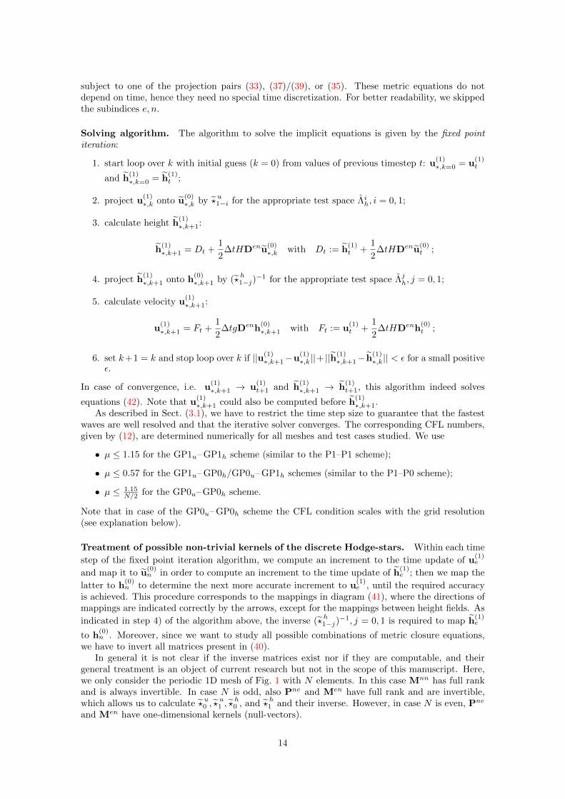
subject to one of the projection pairs (33), (37)/(39), or (35). These metric equations do notdepend on time, hence they need no special time discretization. For better readability, we skippedthe subindices e, n.

Solving algorithm. The algorithm to solve the implicit equations is given by the fixed pointiteration:

1. start loop over k with initial guess (k = 0) from values of previous timestep t: u(1)∗,k=0 = u

(1)t

and h(1)∗,k=0 = h

(1)t ;

2. project u(1)∗,k onto u

(0)∗,k by ?

u1−i for the appropriate test space Λih, i = 0, 1;

3. calculate height h(1)∗,k+1:

h(1)∗,k+1 = Dt +

1

2∆tHDenu

(0)∗,k with Dt := h

(1)t +

1

2∆tHDenu

(0)t ;

4. project h(1)∗,k+1 onto h

(0)∗,k+1 by (?

h1−j)

−1 for the appropriate test space Λjh, j = 0, 1;

5. calculate velocity u(1)∗,k+1:

u(1)∗,k+1 = Ft +

1

2∆tgDenh

(0)∗,k+1 with Ft := u

(1)t +

1

2∆tHDenh

(0)t ;

6. set k+1 = k and stop loop over k if ||u(1)∗,k+1−u

(1)∗,k||+ ||h

(1)∗,k+1− h

(1)∗,k|| < ε for a small positive

ε.

In case of convergence, i.e. u(1)∗,k+1 → u

(1)t+1 and h

(1)∗,k+1 → h

(1)t+1, this algorithm indeed solves

equations (42). Note that u(1)∗,k+1 could also be computed before h

(1)∗,k+1.

As described in Sect. (3.1), we have to restrict the time step size to guarantee that the fastestwaves are well resolved and that the iterative solver converges. The corresponding CFL numbers,given by (12), are determined numerically for all meshes and test cases studied. We use

• µ ≤ 1.15 for the GP1u– GP1h scheme (similar to the P1–P1 scheme);

• µ ≤ 0.57 for the GP1u– GP0h/GP0u– GP1h schemes (similar to the P1–P0 scheme);

• µ ≤ 1.15N/2 for the GP0u– GP0h scheme.

Note that in case of the GP0u– GP0h scheme the CFL condition scales with the grid resolution(see explanation below).

Treatment of possible non-trivial kernels of the discrete Hodge-stars. Within each time

step of the fixed point iteration algorithm, we compute an increment to the time update of u(1)e

and map it to u(0)n in order to compute an increment to the time update of h

(1)e ; then we map the

latter to h(0)n to determine the next more accurate increment to u

(1)e , until the required accuracy

is achieved. This procedure corresponds to the mappings in diagram (41), where the directions ofmappings are indicated correctly by the arrows, except for the mappings between height fields. As

indicated in step 4) of the algorithm above, the inverse (?h1−j)

−1, j = 0, 1 is required to map h(1)e

to h(0)n . Moreover, since we want to study all possible combinations of metric closure equations,

we have to invert all matrices present in (40).In general it is not clear if the inverse matrices exist nor if they are computable, and their

general treatment is an object of current research but not in the scope of this manuscript. Here,we only consider the periodic 1D mesh of Fig. 1 with N elements. In this case Mnn has full rankand is always invertible. In case N is odd, also Pne and Men have full rank and are invertible,which allows us to calculate ?

u0 , ?

u1 , ?

h0 , and ?

h1 and their inverse. However, in case N is even, Pne

and Men have one-dimensional kernels (null-vectors).

14

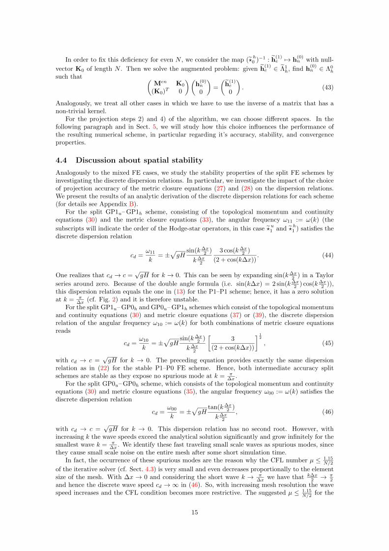
In order to fix this deficiency for even N , we consider the map (?h0 )−1 : h

(1)e 7→ h

(0)n with null-

vector K0 of length N . Then we solve the augmented problem: given h(1)e ∈ Λ1

h, find h(0)n ∈ Λ0

h

such that (Men K0

(K0)T 0

)(h

(0)n

0

)=

(h

(1)e

0

). (43)

Analogously, we treat all other cases in which we have to use the inverse of a matrix that has anon-trivial kernel.

For the projection steps 2) and 4) of the algorithm, we can choose different spaces. In thefollowing paragraph and in Sect. 5, we will study how this choice influences the performance ofthe resulting numerical scheme, in particular regarding it’s accuracy, stability, and convergenceproperties.

4.4 Discussion about spatial stability

Analogously to the mixed FE cases, we study the stability properties of the split FE schemes byinvestigating the discrete dispersion relations. In particular, we investigate the impact of the choiceof projection accuracy of the metric closure equations (27) and (28) on the dispersion relations.We present the results of an analytic derivation of the discrete dispersion relations for each scheme(for details see Appendix B).

For the split GP1u– GP1h scheme, consisting of the topological momentum and continuityequations (30) and the metric closure equations (33), the angular frequency ω11 := ω(k) (the

subscripts will indicate the order of the Hodge-star operators, in this case ?u1 and ?

h1 ) satisfies the

discrete dispersion relation

cd =ω11

k= ±

√gH

sin(k∆x2 )

k∆x2

3 cos(k∆x2 )

(2 + cos(k∆x)). (44)

One realizes that cd → c =√gH for k → 0. This can be seen by expanding sin(k∆x

2 ) in a Taylor

series around zero. Because of the double angle formula (i.e. sin(k∆x) = 2 sin(k∆x2 ) cos(k∆x

2 )),this dispersion relation equals the one in (13) for the P1–P1 scheme; hence, it has a zero solutionat k = π

∆x (cf. Fig. 2) and it is therefore unstable.For the split GP1u– GP0h and GP0u– GP1h schemes which consist of the topological momentum

and continuity equations (30) and metric closure equations (37) or (39), the discrete dispersionrelation of the angular frequency ω10 := ω(k) for both combinations of metric closure equationsreads

cd =ω10

k= ±

√gH

sin(k∆x2 )

k∆x2

[3

(2 + cos(k∆x))

] 12

, (45)

with cd → c =√gH for k → 0. The preceding equation provides exactly the same dispersion

relation as in (22) for the stable P1–P0 FE scheme. Hence, both intermediate accuracy splitschemes are stable as they expose no spurious mode at k = π

∆x .For the split GP0u– GP0h scheme, which consists of the topological momentum and continuity

equations (30) and metric closure equations (35), the angular frequency ω00 := ω(k) satisfies thediscrete dispersion relation

cd =ω00

k= ±

√gH

tan(k∆x2 )

k∆x2

, (46)

with cd → c =√gH for k → 0. This dispersion relation has no second root. However, with

increasing k the wave speeds exceed the analytical solution significantly and grow infinitely for thesmallest wave k = π

∆x . We identify these fast traveling small scale waves as spurious modes, sincethey cause small scale noise on the entire mesh after some short simulation time.

In fact, the occurrence of these spurious modes are the reason why the CFL number µ ≤ 1.15N/2

of the iterative solver (cf. Sect. 4.3) is very small and even decreases proportionally to the elementsize of the mesh. With ∆x → 0 and considering the short wave k → π

∆x we have that k∆x2 → π

2and hence the discrete wave speed cd →∞ in (46). So, with increasing mesh resolution the wavespeed increases and the CFL condition becomes more restrictive. The suggested µ ≤ 1.15

N/2 for the

15

1

2

3

1 2 3

ω11

ω10

ω00

ω

k∆x

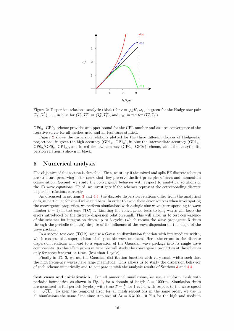
Figure 2: Dispersion relations: analytic (black) for c =√gH, ω11 in green for the Hodge-star pair

(?u1 , ?

h1 ), ω10 in blue for (?

u1 , ?

h0 ) or (?

u0 , ?

h1 ), and ω00 in red for (?

u0 , ?

h0 ).

GP0u– GP0h scheme provides an upper bound for the CFL number and assures convergence of theiterative solver for all meshes used and all test cases studied.

Figure 2 shows the dispersion relations plotted for the three different choices of Hodge-starprojections: in green the high accuracy (GP1u– GP1h), in blue the intermediate accuracy (GP1u–GP0h/GP0u– GP1h), and in red the low accuracy (GP0u– GP0h) scheme, while the analytic dis-persion relation is shown in black.

5 Numerical analysis

The objective of this section is threefold. First, we study if the mixed and split FE discrete schemesare structure-preserving in the sense that they preserve the first principles of mass and momentumconservation. Second, we study the convergence behavior with respect to analytical solutions ofthe 1D wave equations. Third, we investigate if the schemes represent the corresponding discretedispersion relations correctly.

As discussed in sections 3 and 4.4, the discrete dispersion relations differ from the analyticalones, in particular for small wave numbers. In order to avoid these error sources when investigatingthe convergence properties, we perform simulations with a single sine wave (corresponding to wavenumber k = 1) in test case (TC) 1. Limiting the convergence tests to long waves will keep theerrors introduced by the discrete dispersion relation small. This will allow us to test convergenceof the schemes for integration times up to 5 cycles (which means the wave propagates 5 timesthrough the periodic domain), despite of the influence of the wave dispersion on the shape of thewave package.

In a second test case (TC 2), we use a Gaussian distribution function with intermediate width,which consists of a superposition of all possible wave numbers. Here, the errors in the discretedispersion relations will lead to a separation of the Gaussian wave package into its single wavecomponents. As this effect grows in time, we will study the convergence properties of the schemesonly for short integration times (less than 1 cycle).

Finally in TC 3, we use the Gaussian distribution function with very small width such thatthe high frequency waves have large magnitude. This allows us to study the dispersion behaviorof each scheme numerically and to compare it with the analytic results of Sections 3 and 4.4.

Test cases and initialization. For all numerical simulations, we use a uniform mesh withperiodic boundaries, as shown in Fig. 1, for a domain of length L = 1000 m. Simulation timesare measured in full periods (cycles) with time T = L

c for 1 cycle, with respect to the wave speedc =

√gH. To keep the temporal error for all mesh resolutions in the same order, we use in

all simulations the same fixed time step size of ∆t = 6.3102 · 10−04 s for the high and medium

16

accuracy, and ∆t = 12006.3102 · 10−04 s for the low accuracy schemes. These values follow from the

CFL number presented in Sect. 4.3 and from the grid spacing of the highest resolved mesh applied.We use the following analytical solutions of the 1D wave equations with x ∈ [0, L] and t ∈ R

as initializations at time t = 0 and to determine the convergence rates:

Analytical solution for TC 1; single sine wave:

h(x, t) = H +∆H

2sin

(2π

L

(x− ct

))+

∆H

2sin

(2π

L

(x+ ct

)),

u(x, t) =c∆H

2Hsin

(2π

L

(x− ct

))− c∆H

2Hsin

(2π

L

(x+ ct

)),

(47)

with parameters: c =√gH, H = 1000 m, ∆H = 75 , and gravitational acceleration g = 9.81 m/s2.

Analytical solution for TC 2/TC 3; Gaussian distribution with intermediate/small width:

h(x, t) = H +∆H

2e−(

∆w2π sin

(πL (x−ct−xc)

))2

+∆H

2e−(

∆w2π sin

(πL (x+ct−xc)

))2

,

u(x, t) = +c∆H

2He−(

∆w2π sin

(πL (x−ct−xc)

))2

− c∆H

2He−(

∆w2π sin

(πL (x+ct−xc)

))2

,

(48)

with parameters: ∆w = 40, xc = 12L. For TC 3, we use the preceding analytical solution with

very small width by setting ∆w = 1000.A direct calculation shows that both analytical expressions are indeed solutions of the 1D wave

equations (2) or (3). To initialize the discrete schemes, we project the functions h(x, 0) and u(x, 0)onto either the piecewise constant or piecewise linear FE spaces (analogously to Sect. 3 and 4).

Structure-preserving nature of the split schemes. As shown in Sect. 4.2, the split FEschemes are structure-preserving in the sense that the corresponding discrete sets of equationspreserve the splitting into topological and metric parts. Here, we illustrate that these discreteequations also fulfill the first principles of mass and momentum conservation.

In the continuous case with solutions of the wave equations for velocity u(x, t) and heighth(x, t), we define the mass m(t) of the water column and it’s momentum p(t) by

m(t) :=

∫L

h(x, t)dx, p(t) :=

∫L

h(x, t)u(x, t)dx. (49)

In fact, the first principles of mass and momentum conservation allow for the derivation of momen-tum and continuity equations (see e.g. [5]). Therefore, we require our structure preserving schemesto conserve these principles discretely.

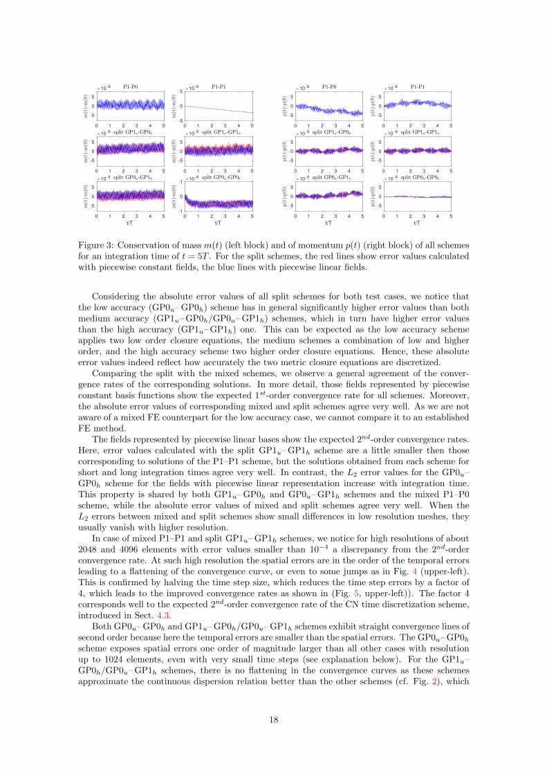
In Fig. 3, we present relative errors for mass and momentum with respect to the correspondinginitial values for all schemes. The results are determined using TC 2 for an integration time oft = 5T on a mesh with 1024 elements for the time step sizes mentioned above. For other meshresolutions and time step sizes, these values remain conserved at the same order of accuracy. Moreprecisely, all schemes expose a mass conservation error (left block) at the order of 10−9 with theunstable P1–P1 FE scheme being the only exception with an error of approx. 10−6. The error inthe momentum (right block) is of the order of 10−9 for all schemes.

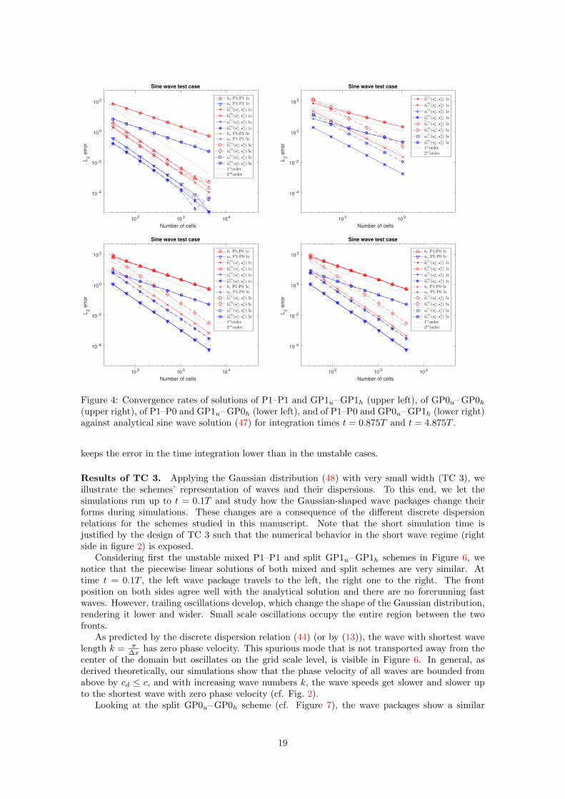
Results for TC 1 and TC 2. Figure 4 shows convergence towards the analytical sine wavesolutions (47) for integration times t = 0.875T and t = 4.875T . Similarly, in Figure 5 convergencesto the analytical Gaussian-shaped solutions (48) for integration times t = 0.125T and t = 0.875Tare given. To determine convergence rates valid for any smooth solution given in the form ofequations (47) and (48), we use values for t that are not multiples of T/4 such that neither heightnor velocity solutions coincide with constant functions.

The reduction in integration time from about 5 cycles for TC 1 down to about 1 cycle forTC 2 is a consequence of the errors caused by the discrete dispersion relations. These lead toa deformation of the Gaussian-shaped wave package and to the development of high oscillatorywaves, which prevents us from determining convergence rates in case of long integration times.

17

0 1 2 3 4 5

-5

0

5

m(t)-m(0)

×10-9 P1-P0

0 1 2 3 4 5

-5

0

5

m(t)-m(0)

×10-9 split GP1u-GP0h

0 1 2 3 4 5

t/T

-5

0

5

m(t)-m(0)

×10-9 split GP0u-GP1h

0 1 2 3 4 5

-5

0

5

m(t)-m(0)

×10-6 P1-P1

0 1 2 3 4 5

-5

0

5

m(t)-m(0)

×10-9 split GP1u-GP1h

0 1 2 3 4 5

t/T

-1

0

1

m(t)-m(0)

×10-8 split GP0u-GP0h

0 1 2 3 4 5

-5

0

5

p(t)-p(0)

×10-9 P1-P0

0 1 2 3 4 5

-5

0

5

p(t)-p(0)

×10-9 split GP1u-GP0h

0 1 2 3 4 5

t/T

-5

0

5

p(t)-p(0)

×10-9 split GP0u-GP1h

0 1 2 3 4 5

-5

0

5

p(t)-p(0)

×10-9 P1-P1

0 1 2 3 4 5

-5

0

5

p(t)-p(0)

×10-9 split GP1u-GP1h

0 1 2 3 4 5

t/T

-5

0

5

p(t)-p(0)

×10-9 split GP0u-GP0h

Figure 3: Conservation of mass m(t) (left block) and of momentum p(t) (right block) of all schemesfor an integration time of t = 5T . For the split schemes, the red lines show error values calculatedwith piecewise constant fields, the blue lines with piecewise linear fields.

Considering the absolute error values of all split schemes for both test cases, we notice thatthe low accuracy (GP0u– GP0h) scheme has in general significantly higher error values than bothmedium accuracy (GP1u– GP0h/GP0u– GP1h) schemes, which in turn have higher error valuesthan the high accuracy (GP1u– GP1h) one. This can be expected as the low accuracy schemeapplies two low order closure equations, the medium schemes a combination of low and higherorder, and the high accuracy scheme two higher order closure equations. Hence, these absoluteerror values indeed reflect how accurately the two metric closure equations are discretized.

Comparing the split with the mixed schemes, we observe a general agreement of the conver-gence rates of the corresponding solutions. In more detail, those fields represented by piecewiseconstant basis functions show the expected 1st-order convergence rate for all schemes. Moreover,the absolute error values of corresponding mixed and split schemes agree very well. As we are notaware of a mixed FE counterpart for the low accuracy case, we cannot compare it to an establishedFE method.

The fields represented by piecewise linear bases show the expected 2nd-order convergence rates.Here, error values calculated with the split GP1u– GP1h scheme are a little smaller then thosecorresponding to solutions of the P1–P1 scheme, but the solutions obtained from each scheme forshort and long integration times agree very well. In contrast, the L2 error values for the GP0u–GP0h scheme for the fields with piecewise linear representation increase with integration time.This property is shared by both GP1u– GP0h and GP0u– GP1h schemes and the mixed P1–P0scheme, while the absolute error values of mixed and split schemes agree very well. When theL2 errors between mixed and split schemes show small differences in low resolution meshes, theyusually vanish with higher resolution.

In case of mixed P1–P1 and split GP1u– GP1h schemes, we notice for high resolutions of about2048 and 4096 elements with error values smaller than 10−4 a discrepancy from the 2nd-orderconvergence rate. At such high resolution the spatial errors are in the order of the temporal errorsleading to a flattening of the convergence curve, or even to some jumps as in Fig. 4 (upper-left).This is confirmed by halving the time step size, which reduces the time step errors by a factor of4, which leads to the improved convergence rates as shown in (Fig. 5, upper-left)). The factor 4corresponds well to the expected 2nd-order convergence rate of the CN time discretization scheme,introduced in Sect. 4.3.

Both GP0u– GP0h and GP1u– GP0h/GP0u– GP1h schemes exhibit straight convergence lines ofsecond order because here the temporal errors are smaller than the spatial errors. The GP0u– GP0hscheme exposes spatial errors one order of magnitude larger than all other cases with resolutionup to 1024 elements, even with very small time steps (see explanation below). For the GP1u–GP0h/GP0u– GP1h schemes, there is no flattening in the convergence curves as these schemesapproximate the continuous dispersion relation better than the other schemes (cf. Fig. 2), which

18

102

103

104

Number of cells

10-4

10-2

100

102

L2 e

rro

rSine wave test case

hn P1-P1 1cun P1-P1 1c

h(1)e (⋆u1 , ⋆

h1 ) 1c

h(0)n (⋆u1 , ⋆

h1 ) 1c

u(1)e (⋆u1 , ⋆

h1 ) 1c

u(0)n (⋆u1 , ⋆

h1 ) 1c

hn P1-P1 5cun P1-P1 5c

h(1)e (⋆u1 , ⋆

h1 ) 5c

h(0)n (⋆u1 , ⋆

h1 ) 5c

u(1)e (⋆u1 , ⋆

h1 ) 5c

u(0)n (⋆u1 , ⋆

h1 ) 5c

1storder

2ndorder

102

103

Number of cells

10-4

10-2

100

102

L2 e

rro

r

Sine wave test case

h(1)e (⋆u0 , ⋆

h0 ) 1c

h(0)n (⋆u0 , ⋆

h0 ) 1c

u(1)e (⋆u0 , ⋆

h0 ) 1c

u(0)n (⋆u0 , ⋆

h0 ) 1c

h(1)e (⋆u0 , ⋆

h0 ) 5c

h(0)n (⋆u0 , ⋆

h0 ) 5c

u(1)e (⋆u0 , ⋆

h0 ) 5c

u(0)n (⋆u0 , ⋆

h0 ) 5c

1storder

2ndorder

102

103

104

Number of cells

10-4

10-2

100

102

L2 e

rro

r

Sine wave test case

he P1-P0 1cun P1-P0 1c

h(1)e (⋆u1 , ⋆

h0 ) 1c

h(0)n (⋆u1 , ⋆

h0 ) 1c

u(1)e (⋆u1 , ⋆

h0 ) 1c

u(0)n (⋆u1 , ⋆

h0 ) 1c

he P1-P0 5cun P1-P0 5c

h(1)e (⋆u1 , ⋆

h0 ) 5c

h(0)n (⋆u1 , ⋆

h0 ) 5c

u(1)e (⋆u1 , ⋆

h0 ) 5c

u(0)n (⋆u1 , ⋆

h0 ) 5c

1storder

2ndorder

102

103

104

Number of cells

10-4

10-2

100

102

L2 e

rro

r

Sine wave test case

he P1-P0 1cun P1-P0 1c

h(1)e (⋆u0 , ⋆

h1 ) 1c

h(0)n (⋆u0 , ⋆

h1 ) 1c

u(1)e (⋆u0 , ⋆

h1 ) 1c

u(0)n (⋆u0 , ⋆

h1 ) 1c

he P1-P0 5cun P1-P0 5c

h(1)e (⋆u0 , ⋆

h1 ) 5c

h(0)n (⋆u0 , ⋆

h1 ) 5c

u(1)e (⋆u0 , ⋆

h1 ) 5c

u(0)n (⋆u0 , ⋆

h1 ) 5c

1storder

2ndorder

Figure 4: Convergence rates of solutions of P1–P1 and GP1u– GP1h (upper left), of GP0u– GP0h(upper right), of P1–P0 and GP1u– GP0h (lower left), and of P1–P0 and GP0u– GP1h (lower right)against analytical sine wave solution (47) for integration times t = 0.875T and t = 4.875T .

keeps the error in the time integration lower than in the unstable cases.

Results of TC 3. Applying the Gaussian distribution (48) with very small width (TC 3), weillustrate the schemes’ representation of waves and their dispersions. To this end, we let thesimulations run up to t = 0.1T and study how the Gaussian-shaped wave packages change theirforms during simulations. These changes are a consequence of the different discrete dispersionrelations for the schemes studied in this manuscript. Note that the short simulation time isjustified by the design of TC 3 such that the numerical behavior in the short wave regime (rightside in figure 2) is exposed.

Considering first the unstable mixed P1–P1 and split GP1u– GP1h schemes in Figure 6, wenotice that the piecewise linear solutions of both mixed and split schemes are very similar. Attime t = 0.1T , the left wave package travels to the left, the right one to the right. The frontposition on both sides agree well with the analytical solution and there are no forerunning fastwaves. However, trailing oscillations develop, which change the shape of the Gaussian distribution,rendering it lower and wider. Small scale oscillations occupy the entire region between the twofronts.

As predicted by the discrete dispersion relation (44) (or by (13)), the wave with shortest wavelength k = π

∆x has zero phase velocity. This spurious mode that is not transported away from thecenter of the domain but oscillates on the grid scale level, is visible in Figure 6. In general, asderived theoretically, our simulations show that the phase velocity of all waves are bounded fromabove by cd ≤ c, and with increasing wave numbers k, the wave speeds get slower and slower upto the shortest wave with zero phase velocity (cf. Fig. 2).

Looking at the split GP0u– GP0h scheme (cf. Figure 7), the wave packages show a similar

19

102

103

104

Number of cells

10-4

10-2

100

102

L2 e

rro

rGaussian distribution test case

hn P1-P1 0.1cun P1-P1 0.1c

h(1)e (⋆u1 , ⋆

h1 ) 0.1c

h(0)n (⋆u1 , ⋆

h1 ) 0.1c

u(1)e (⋆u1 , ⋆

h1 ) 0.1c

u(0)n (⋆u1 , ⋆

h1 ) 0.1c

hn P1-P1 0.9cun P1-P1 0.9c

h(1)e (⋆u1 , ⋆

h1 ) 0.9c

h(0)n (⋆u1 , ⋆

h1 ) 0.9c

u(1)e (⋆u1 , ⋆

h1 ) 0.9c

u(0)n (⋆u1 , ⋆

h1 ) 0.9c

h(0)n (⋆u1 , ⋆

h1 )0.9c ∆t/2

u(0)n (⋆u1 , ⋆

h1 )0.9c ∆t/2

1storder

2ndorder

102

103

Number of cells

10-4

10-2

100

102

L2 e

rro

r

Gaussian distribution test case

h(1)e (⋆u0 , ⋆

h0 ) 0.1c

h(0)n (⋆u0 , ⋆

h0 ) 0.1c

u(1)e (⋆u0 , ⋆

h0 ) 0.1c

u(0)n (⋆u0 , ⋆

h0 ) 0.1c

h(1)e (⋆u0 , ⋆

h0 ) 0.9c

h(0)n (⋆u0 , ⋆

h0 ) 0.9c

u(1)e (⋆u0 , ⋆

h0 ) 0.9c

u(0)n (⋆u0 , ⋆

h0 ) 0.9c

1storder

2ndorder

102

103

104

Number of cells

10-4

10-2

100

102

L2 e

rro

r

Gaussian distribution test case

he P1-P0 0.1cun P1-P0 0.1c

h(1)e (⋆u1 , ⋆

h0 ) 0.1c

h(0)n (⋆u1 , ⋆

h0 ) 0.1c

u(1)e (⋆u1 , ⋆

h0 ) 0.1c

u(0)n (⋆u1 , ⋆

h0 ) 0.1c

he P1-P0 0.9cun P1-P0 0.9c

h(1)e (⋆u1 , ⋆

h0 ) 0.9c

h(0)n (⋆u1 , ⋆

h0 ) 0.9c

u(1)e (⋆u1 , ⋆

h0 ) 0.9c

u(0)n (⋆u1 , ⋆

h0 ) 0.9c

1storder

2ndorder

102

103

104

Number of cells

10-4

10-2

100

102

L2 e

rro

r

Gaussian distribution test case

he P1-P0 0.1cun P1-P0 0.1c

h(1)e (⋆u0 , ⋆

h1 ) 0.1c

h(0)n (⋆u0 , ⋆

h1 ) 0.1c

u(1)e (⋆u0 , ⋆

h1 ) 0.1c

u(0)n (⋆u0 , ⋆

h1 ) 0.1c

he P1-P0 0.9cun P1-P0 0.9c

h(1)e (⋆u0 , ⋆

h1 ) 0.9c

h(0)n (⋆u0 , ⋆

h1 ) 0.9c

u(1)e (⋆u0 , ⋆

h1 ) 0.9c

u(0)n (⋆u0 , ⋆

h1 ) 0.9c

1storder

2ndorder

Figure 5: Convergence rates of solutions of P1–P1 and GP1u– GP1h (upper left), of GP0u– GP0h(upper right), of P1–P0 and GP1u– GP0h (lower left), and of P1–P0 and GP0u– GP1h (lower right)against analytical Gaussian wave solution (48) for integration times t = 0.125T and t = 0.875T .

general behavior as in the previous case. However, the differing discrete dispersion relation (46)leads to differently deformed Gaussian-shaped wave packages compared to the previous unstableschemes. As above, the peaks become smaller and wider. However, in the GP0u– GP0h schemethe central part between the packages is free from high frequency modes, which indicates thatthe scheme does not support a standing spurious mode. On the other hand the high frequencyspurious waves occur outside the central part, hence the scheme supports a fast traveling spuriousmode. In fact, all waves travel with speeds equal to or larger than c, the analytically correct wavespeed, and increase with wave number k up to very large wave speeds. This is why we find wavesoccupying the entire outer region, and why our time step size is so much smaller when comparedto the other schemes (cf. Sect. 4.4). This observation agrees very well with the discrete dispersionrelation for the split GP0u– GP0h scheme shown in Fig. 2.

Let us finally study simulations of TC 3 performed with the mixed P1–P0, the split GP1u–GP0h, and the split GP0u– GP1h schemes. First of all we note that the solutions of the P1–P0and of both split schemes agree very well. This can be inferred from Figures 8 and 9, in which thesolutions of the P1–P0 scheme (green lines) and those of the split schemes (blue and red lines) showonly tiny differences. Again, propagation directions are correct, while the peaks become smallerand wider. In between the peaks, no high frequency waves occupy the central region, similarly tothe split GP0u– GP0h scheme. In contrast to the latter however, the high frequency waves do notoccupy the entire outer region but only some parts directly in front of the traveling wave packages.This reflects very well the theoretical findings described by the discrete dispersion relation (45),which states that all waves travel equal to, or faster then c, but not faster than about 1.1c (cf.Fig. 2).

20

350 400 450 500

m

999.5

1000

1000.5

1001

1001.5

1002m

h(x, 0)h(x, t)hn P1-P1

h(1)e (⋆u1 , ⋆

h1 )

h(0)n (⋆u1 , ⋆

h1 )

0 200 400 600 800 1000

m

990

995

1000

1005

1010

1015

1020

1025

1030

1035

1040

m

350 400 450 500

m

-0.5

-0.4

-0.3

-0.2

-0.1

0

0.1

m/s

u(x, 0)u(x, t)un P1-P1

u(1)e (⋆u1 , ⋆

h1 )

u(0)n (⋆u1 , ⋆

h1 ) 0 200 400 600 800 1000

m

-3

-2

-1

0

1

2

3

m/s

Figure 6: Illustration of the effects of the discrete dispersion relation (44) of the unstable P1–P1and GP1u– GP1h schemes on Gaussian-shaped height and velocity peaks after a simulation timeof t = 0.1T .

350 400 450 500

m

999.5

1000

1000.5

1001

1001.5

1002

m

h(x, 0)h(x, t)

h(1)e (⋆u0 , ⋆

h0 )

h(0)n (⋆u0 , ⋆

h0 )

0 200 400 600 800 1000

m

990

995

1000

1005

1010

1015

1020

1025

1030

1035

1040

m

0 50 100 150 200 250 300 350 400

m

-0.5

-0.4

-0.3

-0.2

-0.1

0

0.1

m/s

u(x, 0)u(x, t)

u(1)e (⋆u0 , ⋆

h0 )

u(0)n (⋆u0 , ⋆

h0 )

0 200 400 600 800 1000

m

-3

-2

-1

0

1

2

3

m/s

Figure 7: Illustration of the effects of the discrete dispersion relation (46) of the GP0u– GP0hscheme on Gaussian-shaped height and velocity peaks after a simulation time of t = 0.1T .

6 Summary, Conclusions, Outlook

We developed a new finite element (FE) discretization framework based on the split 1D waveequations (3) with the long term objective to apply this framework to derive structure-preservingdiscretizations for Geophysical Fluid Dynamics (GFD) [5]. The splitting of these covariant equa-tions into topological momentum/continuity equations and metric-dependent closure equationsrelies on the introduction of additional differential forms (DF). These establish pairs with the orig-inal DFs, which are connected by the Hodge-star operator. By providing proper FE spaces for allDFs such that the differential operators (here gradient and divergence) hold in strong form, oursplit FE framework provides discretizations that preserve geometrical structure. In particular, thediscrete momentum and continuity equations are metric-free and hold in strong form (no partialintegration is required). They are therefore exact up to the errors introduced by the trivial pro-jections into the correspond FE spaces. Additional errors are however introduced by the discretemetric-dependent closure equations that provide approximations to the Hodge-star operator bynontrivial Galerkin projections (GP).

Requirements from structure preservation together with our objective to develop a lowest-order scheme for the split 1D wave equations impose certain conditions on the choice of FE spacesthat approximate the corresponding DFs. In detail, both topological equations are projectedonto piecewise constant spaces, whereas each of the two metric equations is projected onto bothpiecewise constant and piecewise linear spaces. Although this gives four possible realizations,

21

350 400 450 500

m

999.5

1000

1000.5

1001

1001.5

1002m

h(x, 0)h(x, t)he P1-P0

h(1)e (⋆u1 , ⋆

h0 )

h(0)n (⋆u1 , ⋆

h0 )

0 200 400 600 800 1000

m

990

995

1000

1005

1010

1015

1020

1025

1030

1035

1040

m

0 50 100 150 200 250 300 350 400

m

-0.5

-0.4

-0.3

-0.2

-0.1

0

0.1

0.2

m/s

u(x, 0)u(x, t)un P1-P0

u(1)e (⋆u1 , ⋆

h0 )

u(0)n (⋆u1 , ⋆

h0 )

0 200 400 600 800 1000

m

-3

-2

-1

0

1

2

3

m/s

Figure 8: Illustration of the effects of the discrete dispersion relation (45) of the stable P1–P0and GP1u– GP0h schemes on Gaussian-shaped height and velocity peaks after a simulation timeof t = 0.1T .

350 400 450 500

m

999.5

1000

1000.5

1001

1001.5

1002

m

h(x, 0)h(x, t)he P1-P0

h(1)e (⋆u0 , ⋆

h1 )

h(0)n (⋆u0 , ⋆

h1 )

0 200 400 600 800 1000

m

990

995

1000

1005

1010

1015

1020

1025

1030

1035

1040

m

0 50 100 150 200 250 300 350 400

m

-0.5

-0.4

-0.3

-0.2

-0.1

0

0.1

0.2

m/s

u(x, 0)u(x, t)un P1-P0

u(1)e (⋆u0 , ⋆

h1 )

u(0)n (⋆u0 , ⋆

h1 )

0 200 400 600 800 1000

m

-3

-2

-1

0

1

2

3

m/s

Figure 9: Illustration of the effects of the discrete dispersion relation (45) of the stable P1–P0and GP0u– GP1h schemes on Gaussian-shaped height and velocity peaks after a simulation timeof t = 0.1T .

we find in principle three classes of schemes: a high accuracy scheme (GP1– GP1), in which theGalerkin projections map onto piecewise linear (GP1) spaces, a low accuracy scheme (GP0– GP0),in which the Galerkin projections map onto piecewise constant (GP0) spaces, and two mediumaccuracy schemes (GP1– GP0), in which one Galerkin projection maps onto piecewise linear, theother to piecewise constant space.

A comparison to conventional methods, the unstable P1–P1 scheme that applies piecewiselinear (P1) spaces to approximate both velocity and height fields, and the stable P1–P0 schemethat approximates the velocity by a piecewise linear and the height by a piecewise constant (P0)field, was performed with respect to conservation of mass and momentum, dispersion relations,and convergence behavior. Analytical derivations showed that the discrete dispersion relations ofthe unstable P1–P1 and GP1– GP1 schemes as well as of the stable P1–P0 and both GP1– GP0schemes coincide, in spite of the differences in how they are derived. In particular, the GP1– GP1scheme and the P1–P1 scheme share the problem of permitting spurious modes, whereas the stableP1–P0 scheme and the two GP1– GP0 schemes are free of such modes.

The piecewise linear fields of P1–P1 and GP1– GP1 schemes show more or less the same con-vergence rates of second order. Applying four instead of only two FE spaces, we illustrated thatthe piecewise constant fields, present only in the split schemes, showed the expected first orderconvergence rate. Similarly, the corresponding fields of the P1–P0 and both GP1– GP0 schemesagree in their convergence behavior. Both piecewise constant height fields show first order and

22

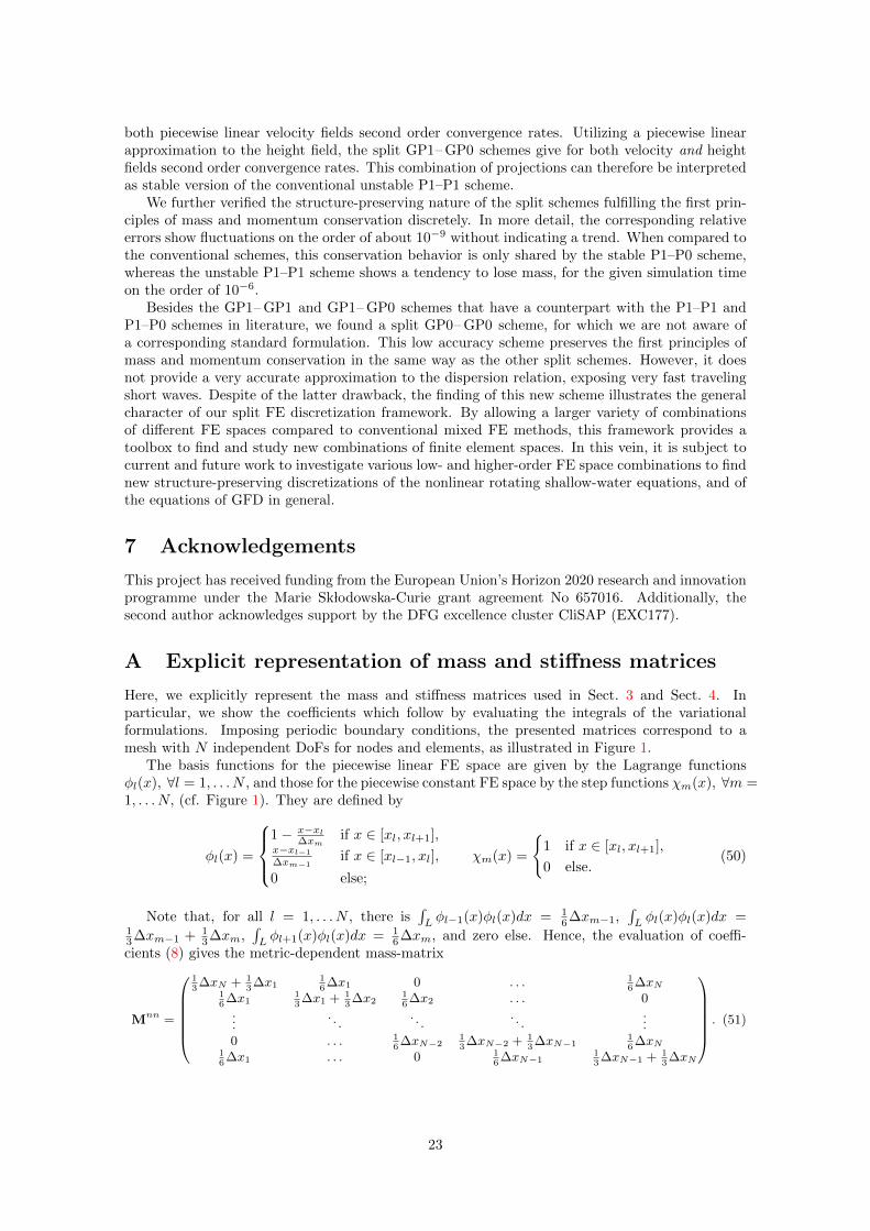
both piecewise linear velocity fields second order convergence rates. Utilizing a piecewise linearapproximation to the height field, the split GP1– GP0 schemes give for both velocity and heightfields second order convergence rates. This combination of projections can therefore be interpretedas stable version of the conventional unstable P1–P1 scheme.

We further verified the structure-preserving nature of the split schemes fulfilling the first prin-ciples of mass and momentum conservation discretely. In more detail, the corresponding relativeerrors show fluctuations on the order of about 10−9 without indicating a trend. When compared tothe conventional schemes, this conservation behavior is only shared by the stable P1–P0 scheme,whereas the unstable P1–P1 scheme shows a tendency to lose mass, for the given simulation timeon the order of 10−6.

Besides the GP1– GP1 and GP1– GP0 schemes that have a counterpart with the P1–P1 andP1–P0 schemes in literature, we found a split GP0– GP0 scheme, for which we are not aware ofa corresponding standard formulation. This low accuracy scheme preserves the first principles ofmass and momentum conservation in the same way as the other split schemes. However, it doesnot provide a very accurate approximation to the dispersion relation, exposing very fast travelingshort waves. Despite of the latter drawback, the finding of this new scheme illustrates the generalcharacter of our split FE discretization framework. By allowing a larger variety of combinationsof different FE spaces compared to conventional mixed FE methods, this framework provides atoolbox to find and study new combinations of finite element spaces. In this vein, it is subject tocurrent and future work to investigate various low- and higher-order FE space combinations to findnew structure-preserving discretizations of the nonlinear rotating shallow-water equations, and ofthe equations of GFD in general.

7 Acknowledgements

This project has received funding from the European Union’s Horizon 2020 research and innovationprogramme under the Marie Sk lodowska-Curie grant agreement No 657016. Additionally, thesecond author acknowledges support by the DFG excellence cluster CliSAP (EXC177).

A Explicit representation of mass and stiffness matrices

Here, we explicitly represent the mass and stiffness matrices used in Sect. 3 and Sect. 4. Inparticular, we show the coefficients which follow by evaluating the integrals of the variationalformulations. Imposing periodic boundary conditions, the presented matrices correspond to amesh with N independent DoFs for nodes and elements, as illustrated in Figure 1.

The basis functions for the piecewise linear FE space are given by the Lagrange functionsφl(x), ∀l = 1, . . . N , and those for the piecewise constant FE space by the step functions χm(x), ∀m =1, . . . N, (cf. Figure 1). They are defined by

φl(x) =

1− x−xl

∆xmif x ∈ [xl, xl+1],

x−xl−1

∆xm−1if x ∈ [xl−1, xl],

0 else;

χm(x) =

{1 if x ∈ [xl, xl+1],

0 else.(50)

Note that, for all l = 1, . . . N , there is∫Lφl−1(x)φl(x)dx = 1

6∆xm−1,∫Lφl(x)φl(x)dx =

13∆xm−1 + 1

3∆xm,∫Lφl+1(x)φl(x)dx = 1

6∆xm, and zero else. Hence, the evaluation of coeffi-cients (8) gives the metric-dependent mass-matrix

Mnn =

13∆xN + 1

3∆x1

16∆x1 0 . . . 1

6∆xN

16∆x1

13∆x1 + 1

3∆x2

16∆x2 . . . 0

.... . .

. . .. . .

...0 . . . 1

6∆xN−2

13∆xN−2 + 1

3∆xN−1

16∆xN

16∆x1 . . . 0 1

6∆xN−1

13∆xN−1 + 1

3∆xN

. (51)

23

Because of the periodic boundary, we identify here and throughout the entire manuscript φ0(x) with

φN (x) and φN+1(x) with φ1(x). Moreover, for all l = 1, . . . N , there is∫Ldφl∓1(x)

dx φl(x)dx = ∓ 12 ,

and zero else. Therefore, the evaluation of coefficients (9) gives the metric-free stiffness matrix

Dnn =

0 1

2 0 . . . 12

− 12 0 1

2 . . . 0...

. . .. . .

. . ....

0 . . . − 12 0 1

212 . . . 0 − 1

2 0

. (52)

Applying the values∫Lχm(x)χm(x) = ∆xm for all m = 1, . . . N , zero else, to evaluate co-

efficients (18) and∫L

dφl/l+1(x)

dx χm(x)dx = −1/1 for all m = 1, . . . N , zero else, to calculate co-efficients (19), there follow the metric-dependent mass-matrix Mee and the metric-free stiffnessmatrix Den:

Mee =

∆x1 0 . . . 0

0 ∆x2 . . . 0...

.... . .

...0 0 . . . ∆xN

, Den =

−1 1 0 . . . 00 −1 1 . . . 0...

.... . .

. . ....

0 0 . . . −1 11 0 . . . 0 −1

,

with Dne = (Den)T .Finally, using the values

∫Lχm−1/m(x)φl(x)dx = 1

2∆xm−1/12∆xm for all l = 1, . . . N , zero else,

the evaluation of coefficients (32) gives the metric-dependent mass-matrix Mne with correspondingmetric-free projection matrix Pne:

Mne =

12∆x1 0 . . . 1

2∆xN12∆x1

12∆x2 . . . 0

.... . .

. . ....

0 . . . 12∆xN−1

12∆xN

, Pne =

12 0 . . . 1

212

12 . . . 0

.... . .

. . ....

0 . . . 12

12

.

B Derivation of the discrete dispersion relations

In this section we present a detailed derivation of the discrete dispersion relations, presented inSect. 3 for the mixed, and in Sect. 4 for the split schemes. For the mixed schemes we mainly followthe approach presented in [23]. For the split schemes, we adapt this approach such that it suits tothe split form of the wave equations.

B.1 The analytical case

To explain the method, we first determine the dispersion relation for the analytical wave equations.As above, we consider the domain L with coordinates x ∈ [0, L] ⊂ R and time variable t ∈ R. Weassume that the solutions can be formulated as periodic in space and time. In more detail, we seekperiodic solutions of the equations (2), i.e. we decompose the solutions like

u(x, t) = u(x)eiωt = ueiωt−ikx, h(x, t) = h(x)eiωt = heiωt−ikx, (53)

in which u, h are constants. ω is the angular frequency and k is the wave number.Applying the first decomposition of (53) with respect to time to evaluate the time derivative

of (2), we obtain equations in harmonic form

iωu(x) + g∂h(x)

∂x= 0, iωh(x) +H

∂u(x)

∂x= 0 . (54)

Using further the second decomposition of (53) in wave vector space with wave vector k, we find(iω igkiHk iω

)(u

h

)= 0 . (55)

24

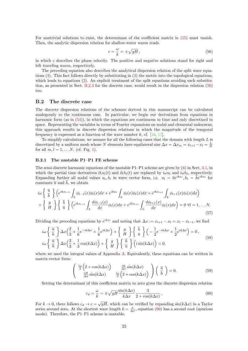
For nontrivial solutions to exist, the determinant of the coefficient matrix in (55) must vanish.Then, the analytic dispersion relation for shallow-water waves reads

c =ω

k= ±

√gH , (56)

in which c describes the phase velocity. The positive and negative solutions stand for right andleft traveling waves, respectively.

The preceding equation also describes the analytical dispersion relation of the split wave equa-tions (3). This fact follows directly by substituting in (3) the metric into the topological equations,which leads to equations (2). An explicit treatment of the split equations avoiding such substitu-tion, as presented in Sect. B.2.3 for the discrete case, would result in the dispersion relation (56)too.

B.2 The discrete case

The discrete dispersion relations of the schemes derived in this manuscript can be calculatedanalogously to the continuous case. In particular, we begin our derivations from equations inharmonic form (as in (54)), in which the equations are continuous in time and only discretized inspace. Representing the variables in terms of Fourier expansions on nodal and elemental unknowns,this approach results in discrete dispersion relations in which the magnitude of the temporalfrequency is expressed as a function of the wave number k, cf. [16, 17].

To simplify calculations, we assume for all the following cases that the domain with length L isdiscretized by a uniform mesh whose N elements have equilateral size ∆x = ∆xm = xl+1−xl = L

Nfor all m, l = 1, . . . N , (cf. Fig. 1).

B.2.1 The unstable P1–P1 FE scheme

The semi-discrete harmonic equations of the unstable P1–P1 scheme are given by (6) in Sect. 3.1, inwhich the partial time derivatives ∂tul(t) and ∂thl(t) are replaced by iωul and iωhl, respectively.Expanding further all nodal values ul, hl in wave vector form, i.e. ul = ueikxl , hl = heikxl forconstants u and h, we obtain

iω

{u

h

}(eikxl−1

∫L

φl−1(x)φl(x)dx+ eikxl∫L

φl(x)φl(x)dx+ eikxl+1

∫L

φl+1(x)φl(x)dx)

+

{gH

}{hu

}(eikxl−1

∫L

dφl−1(x)

dxφl(x)dx+ eikxl+1

∫L

dφl+1(x)

dxφl(x)dx

)= 0 ∀l = 1, . . . N.

(57)

Dividing the preceding equations by eikxl and noting that ∆x := xl+1 − xl = xl − xl−1, we find

iω

{u

h

}∆x(2

3+

1

6e−ik∆x +

1

6eik∆x

)+

{gH

}{hu

}(− 1

2e−ik∆x +

1

2eik∆x

)= 0 ,

iω

{u

h

}∆x(2

3+

1

3cos(k∆x)

)+

{gH

}{hu

}(i sin(k∆x)

)= 0,

(58)

where we used the integral values of Appendix A. Equivalently, these equations can be written inmatrix-vector form: iω

3

(2 + cos(k∆x)

)ig∆x sin(k∆x)

iH∆x sin(k∆x) iω

3

(2 + cos(k∆x)

) ( u

h

)= 0. (59)

Setting the determinant of this coefficient matrix to zero gives the discrete dispersion relation

cd =ω

k= ±

√gH

sin(k∆x)

k∆x

3

2 + cos(k∆x). (60)

For k → 0, there follows cd → c =√gH, which can be verified by expanding sin(k∆x) in a Taylor

series around zero. At the shortest wave length k = π∆x , equation (60) has a second root (spurious

mode). Therefore, the P1–P1 scheme is unstable.

25

B.2.2 The stable P1–P0 FE scheme

In case of the stable P1–P0 scheme introduced in Sect. 3.2, the semi-discrete harmonic equationsare given by (16), with ∂tul(t) and ∂thm(t) replaced by iωul and iωhm, respectively. Here weexpand the variables for all nodes as ul = ueikxl and for all elements as hm = heikxm .

Then, the discrete momentum equation reads

iωu(eikxl−1

∫L

φl−1(x)φl(x)dx+ eikxl∫L

φl(x)φl(x)dx+ eikxl+1

∫L

φl+1(x)φl(x)dx)

− gh(eikxm−1

∫L

χm−1(x)dφl(x)

dxdx+ eikxm

∫L

χm(x)dφl(x)

dxdx)

= 0, ∀ l = 1, . . . N,

(61)

and the continuity equation reads

iωheikxm∫L

χm(x)χm(x)dx+

Hu(eikxl

∫L

dφl(x)

dxχm(x)dx+ eikxl+1

∫L

dφl+1(x)

dxχm(x)dx

)= 0, ∀ m = 1, . . . N.

(62)

Dividing the former equation by eikxl and the latter by eikxm , noting that ∆x2 = xl+1 − xm =

xm − xl−1 on a uniform mesh, and using the integral values of Appendix A, the momentumequation becomes

iωu∆x(2

3+

1

6e−ik∆x +

1

6eik∆x

)+ gh

(− e−ik∆x

2 + eik∆x2

)= 0 ,

iωu∆x(2

3+

1

3cos(k∆x)

)+ gh2i sin

(k

∆x

2

)= 0 ,

(63)

and the continuity equation becomes

iωh∆x+Hu(− e−ik∆x

2 + eik∆x2

)= 0 ,

iωh∆x+Hu2i sin

(k

∆x

2

)= 0 .

(64)

In matrix-vector formulation, the preceding set of discrete equations yields(iω3 (2 + cos(k∆x)) i2g

∆x sin(k∆x2 )

i2H∆x sin(k∆x

2 ) iω

)(u

h

)= 0 . (65)

Setting the determinant of this coefficient matrix to zero results in the discrete dispersionrelation

cd =ω

k= ±

√gH

sin(k∆x2 )

k∆x2

[3

2 + cos(k∆x)

]1/2

. (66)

Also here, cd → c for k → 0. However, in contrast to the unstable P1–P1 scheme, there is nosecond root at shortest wave length k = π

∆x . Instead, the discrete dispersion relation approximateswell the analytical one. Therefore, we consider this scheme as stable.

B.2.3 The split FE schemes

For the split schemes derived in Sect. 4, the semi-discrete harmonic topological equations aregiven by (29), with ∂tum(t) and ∂thm(t) replaced by iωum and iωhm, respectively. Here weexpand the coefficient of velocity and height in wave vector form as follows: at nodal values as

ul = ueikxl , hl = heikxl , and at elemental values as hm = heikxm , um = ueikxm , with constants

u, h, h, and u. We obtain

iω

{u

h

}(eikxm

∫L

χm(x)χm(x)dx)

+

{gH

}{h

u

}(eikxl

∫L

dφl(x)

dxχm(x)dx+ eikxl+1

∫L

dφl+1(x)

dxχm(x)dx

)= 0, ∀m = 1, . . . N.

(67)

26

Dividing the preceding equations by eikxm and using ∆x2 = xl+1−xm = xm−xl−1 and the integral

values of Appendix A, there follows

iω

{u

h

}∆x+

{gH

}{h

u

}(eik

∆x2 − e−ik∆x

2

)= 0 ,

iω

{u

h

}+

{gH

}{h

u

}2i

∆xsin

(k

∆x

2

)= 0 .

(68)

In Sect. 4.2.2, we presented four realizations of discrete metric equations as closure conditions tothe topological equations (30). Here we proceed similarly and derive discrete metric equations thatclose the harmonic equations (68), i.e. we distinguish between high, medium, and low accuracyclosures.

High accuracy closure. The discrete metric closure equations for the high accuracy case aregiven by (31). Representing the variables in wave vector form at nodal and elemental values usingthe expansion as for the topological equations, we obtain{

u

h

}(eikxl−1

∫L

φl−1(x)φl(x)dx+ eikxl∫L

φl(x)φl(x)dx+ eikxl+1

∫L

φl+1(x)φl(x)dx)

=

{u

h

}(eikxm−1

∫L

χm−1(x)φl(x)dx+ eikxm∫L

χm(x)φl(x)dx)∀l = 1, . . . N.

(69)

Dividing the preceding equation by eikxl , using ∆x2 = xl+1 − xm = xm − xl−1, and applying the

integral values of Appendix A, we find{u

h

}∆x(2

3+

1

6e−ik∆x +

1

6eik∆x

)=

{u

h

}∆x

2

(e−ik

∆x2 + eik

∆x2

),

{u

h

}(2

3+

1

3cos(k∆x)

)=

{u

h

}cos

(k

∆x

2

).

(70)

The combination of these latter with the discrete topological equations (68) gives the matrix-vectorequations:

iω i 2g∆x sin(k∆x

2 ) 0 00 0 i 2H

∆x sin(k∆x2 ) iω

− cos(k∆x2 ) 0

(23 + 1

3 cos(k∆x))

0

0(

23 + 1

3 cos(k∆x))

0 − cos(k∆x2 )

u

h

u

h

= 0 . (71)

To find nontrivial solutions of this equation, we set the determinant of this coefficient matrixto zero. There follows the discrete dispersion relation

cd =ω11

k= ±

√gH

sin(k∆x2 )

k∆x2

3 cos(k∆x2 )

(2 + cos(k∆x)). (72)

For k → 0, there follows cd → c. The high accuracy scheme GP1u– GP1h has a root solu-tion at k = π

∆x and is hence unstable. Because of the double angle formula (i.e. sin(k∆x) =

2 sin(k∆x2 ) cos(k∆x

2 )), this dispersion relation equals the one in (60) for the unstable P1–P1 scheme.

Low accuracy closure. In the low accuracy case, the discrete metric equations are given by(34), in which the variables at nodal and elemental values are expanded as for the topologicalequations. Then, {

u

h

}(eikxl

∫L

φl(x)χm(x)dx+ eikxl+1

∫L

φl+1(x)χm(x)dx)

=

{u

h

}eikxm

∫L

χm(x)χm(x)dx, ∀m = 1, . . . N.

(73)

27

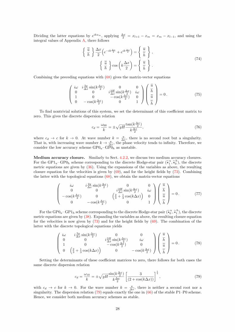
Dividing the latter equations by eikxm , applying ∆x2 = xl+1 − xm = xm − xl−1, and using the

integral values of Appendix A, there follows{u

h

}∆x

2

(e−ik

∆x2 + eik

∆x2

)=

{u

h

},

{u

h

}cos

(k

∆x

2

)=

{u

h

}.

(74)

Combining the preceding equations with (68) gives the matrix-vector equationsiω i 2g

∆x sin(k∆x2 ) 0 0

0 0 i 2H∆x sin(k∆x

2 ) iω1 0 − cos(k∆x

2 ) 00 − cos(k∆x

2 ) 0 1

u

h

u

h

= 0 . (75)

To find nontrivial solutions of this system, we set the determinant of this coefficient matrix tozero. This gives the discrete dispersion relation

cd =ω00

k= ±

√gH

tan(k∆x2 )

k∆x2

, (76)

where cd → c for k → 0. At wave number k = π∆x , there is no second root but a singularity.

That is, with increasing wave number k → π∆x , the phase velocity tends to infinity. Therefore, we

consider the low accuracy scheme GP0u– GP0h as unstable.

Medium accuracy closure. Similarly to Sect. 4.2.2, we discuss two medium accuracy closures.For the GP1u– GP0h scheme corresponding to the discrete Hodge-star pair (?

u1 , ?

h0 ), the discrete

metric equations are given by (36). Using the expansions of the variables as above, the resultingclosure equation for the velocities is given by (69), and for the height fields by (73). Combiningthe latter with the topological equations (68), we obtain the matrix-vector equations

iω i 2g∆x sin(k∆x

2 ) 0 00 0 i 2H

∆x sin(k∆x2 ) iω

− cos(k∆x2 ) 0

(23 + 1

3 cos(k∆x))

0

0 − cos(k∆x2 ) 0 1

u

h

u

h

= 0 . (77)

For the GP0u– GP1h scheme corresponding to the discrete Hodge-star pair (?u0 , ?

h1 ), the discrete

metric equations are given by (38). Expanding the variables as above, the resulting closure equationfor the velocities is now given by (73) and for the height fields by (69). The combination of thelatter with the discrete topological equations yields

iω i 2g∆x sin(k∆x

2 ) 0 00 0 i 2H

∆x sin(k∆x2 ) iω

1 0 − cos(k∆x2 ) 0

0(

23 + 1

3 cos(k∆x))

0 − cos(k∆x2 )

u

h

u

h

= 0 . (78)

Setting the determinants of these coefficient matrices to zero, there follows for both cases thesame discrete dispersion relation

cd =ω10

k= ±

√gH

sin(k∆x2 )

k∆x2

[3

(2 + cos(k∆x))

] 12

, (79)

with cd → c for k → 0. For the wave number k = π∆x , there is neither a second root nor a

singularity. The dispersion relation (79) equals exactly the one in (66) of the stable P1–P0 scheme.Hence, we consider both medium accuracy schemes as stable.

28

Remark. Considering the matrix-vector equations for all four cases, we realize that the first two linesremain unchanged while the second two lines change with the choice of discrete metric equations.Incorporating how the straight and twisted forms are connected, it is the choice of the metricequations that determine – by these last two lines – the schemes’ discrete dispersion relations.

References

[1] Arnold, D. N. [2002], Differential complexes and numerical stability. Proceedings of the In-ternational Congress of Mathematicians, Beijing, 1, 137–157.

[2] Arnold, D. N., Falk, R. S., and Winther, R. [2006], Finite element exterior calculus, homo-logical techniques, and applications. Acta Numerica, 15, 1–155.

[3] Arnold, D. N., Falk, R. S., and Winther, R. [2010], Finite element exterior calculus: fromHodge theory to numerical stability. Bull. Amer. Math. Soc. (N.S.), 47, 281–354.

[4] Bauer, W. [2013], Toward Goal-Oriented R-adaptive Models in Geophysical Fluid Dynam-ics using a Generalized Discretization Approach. PhD thesis, Department of Geosciences,University of Hamburg.

[5] Bauer, W. [2016], A new hierarchically-structured n-dimensional covariant form of rotatingequations of geophysical fluid dynamics, GEM - International Journal on Geomathematics,7(1), 31–101.

[6] Behrens, J. [2006], Adaptive Atmospheric Modeling - Key Techniques in Grid Generation,Data Structures, and Numerical Operations with Applications. Lecture Notes in Computa-tional Science and Engineering, 54, Springer Verlag, Berlin, Heidelberg, doi:10.1007/3-540-33383-5.

[7] Bochev, P. and Hyman, J. [2006], Principles of mimetic discretizations of differential opera-tors. Compatible Spatial Discretizations, The IMA Volumes in Mathematics and its Applica-tions, 142, 89–119.

[8] Boffi, Daniele and Fortin, Michel and Brezzi, Franco [2013], Mixed finite element methods andapplications, Springer series in computational mathematics, Springer, Berlin, Heidelberg.

[9] Bossavit, A. [2001], ’Generalized finite differences’ in computational electromagnetics,Progress In Electromagnetics Research (PIER), 32, 45–64.

[10] Cotter, C.J. and Ham, D.A. and Pain, C.C. and Reich, S. [2009], LBB stability of a mixedGalerkin finite element pair for fluid flow simulations, Journal of Computational Physics.

[11] Cotter, C.J. and McRae, A.T.T. [2014], Compatible finite elements for numerical weatherprediction, arXiv:1401.0616, https://arxiv.org/abs/1401.0616.

[12] Cotter, C.J., Thuburn, J. [2012], A finite element exterior calculus framework for the rotatingshallow-water equations, Journal of Computational Physics, 257(B), 1506–1526.

[13] Desbrun, M., Hirani, A. N., Leok, M., and Marsden, J. E. [2005], Discrete exterior calculus,arXiv:math/0508341v2 [math.DG].

[14] Kreeft, J. J. and Palha, A. and Gerritsma, M. I. [2010], Mimetic spectral element methodfor generalized convection-diffusion problems. In Proceedings of the European Conference onComputational Fluid Dynamics (ECCOMAS CFD).

[15] Lee, J. J., and Winther, R. [2016], Local coderivatives and approximation of Hodge Laplaceproblems, To appear. arXiv preprint 1610.07954, https://arxiv.org/abs/1610.07954.

[16] Le Roux, D. Y. and Rostand, V. and Benoit, P. [2007], Analysis of Numerically InducedOscillations in 2D Finite-Element Shallow-Water Models Part I: Inertia-Gravity Waves SIAMJ. Sci. Comput., 29(1), 331–360.

29

[17] Le Roux, D. Y. and Pouliot, B. [2008], Analysis of Numerically Induced Oscillations in Two-Dimensional Finite-Element Shallow-Water Models Part II: Free Planetary Waves, SIAM J.Sci. Comput., 30(4), 1971–1991.

[18] LeVeque, R. J. [2002], Finite Volume Methods for Hyperbolic Problems, Cambridge Univer-sity Press, ISBN 0-521-81087-6.

[19] Lipnikov, K. and Manzini, G. and Shashkov, M. [2013], Mimetic finite difference method, J.Comput. Phys., 257(B), 1 – 107, http://dx.doi.org/10.1016/j.jcp.2013.07.031..

[20] Logg, A. and Mardal, K.-A. and Wells, G. N., et al. [2012], Automated Solution of DifferentialEquations by the Finite Element Method, Springer, doi:10.1007/978-3-642-23099-8.

[21] Palha, A. and Rebelo, P. P. and Hiemstra, R. and Kreeft, J. and Gerritsma, M. [2014],Physics-compatible discretization techniques on single and dual grids, with application tothe Poisson equation of volume forms, Journal of Computational Physics, 257(B), 1394 –1422.

[22] Pedlosky, J. [1979], Geophysical fluid dynamics. Springer Verlag, New York.

[23] Walters, R. A., Carey, G. F. [1983], Analysis of spurious oscillation modes for the shallow-water and Navier-Stokes equations, Computers and Fluids, 11(1), 51–68.

30