the stability of localized spikes for the 1-d …ward/papers/brus_revise.pdf · have been...
TRANSCRIPT
Under consideration for publication in EJAM 1
The Stability of Localized Spikes for the 1-D Brusselator
Reaction-Diffusion Model
J. C. TZOU, Y. NEC, M. J. WARD
Justin Tzou, Dept. of Engineering Sciences and Applied Mathematics, Northwestern University, 2145 Sheridan Road, Evanston, Illinois,
60208-3125 USA (corresponding author),
Yana Nec and Michael Ward; Department of Mathematics, University of British Columbia, Vancouver, British Columbia, V6T 1Z2, Canada.
(Received 15 January 2013)
In a one-dimensional domain, the stability of localized spike patterns is analyzed for two closely related singularly per-
turbed reaction-diffusion (RD) systems with Brusselator kinetics. For thefirst system, where there is no influx of the inhibitor
on the domain boundary, asymptotic analysis is used to derive a nonlocaleigenvalue problem (NLEP) whose spectrum deter-
mines the linear stability of a multi-spike steady-state solution. Similar to previousNLEP stability analyses of spike patterns
for other RD systems, such as the Gierer-Meinhardt (GM) and Gray-Scott (GS) models, a multi-spike steady-state solution
can become unstable to either a competition or an oscillatory instability depending on the parameter regime. An explicit
result for the threshold value for the initiation of a competition instability, which triggers the annihilation of spikes in a
multi-spike pattern, is derived. Alternatively, in the parameter regime when a Hopf bifurcation occurs, it is shown from a
numerical study of the NLEP that anasynchronous, rather than synchronous, oscillatory instability of the spike amplitudes
can be the dominant instability. The existence of robust asynchronous temporal oscillations of the spike amplitudes has not
been predicted from NLEP stability studies of other RD systems. For the second system, where there is an influx of inhibitor
from the domain boundaries, an NLEP stability analysis of a quasi-steady-state two-spike pattern reveals the possibility of
dynamic bifurcations leading to either a competition or an oscillatory instability ofthe spike amplitudes depending on the
parameter regime. It is shown that the novelasynchronousoscillatory instability mode can again be the dominant instability.
For both Brusselator systems, the detailed stability results from NLEP theoryare confirmed by rather extensive numerical
computations of the full PDE system.
Key words: Brusselator, singular perturbations, quasi-equilibria,nonlocal eigenvalue problem, Hopf bifurcation, asyn-chronous oscillatory instability, dynamically triggeredinstability.
1 Introduction
Spatially localized patterns arise from a wide variety of reaction-diffusion systems, with applications to chemical
dynamics and biological modelling (cf. [29]), the spatial distribution of urban crime (cf. [24, 14]), electronic gas-
discharge systems (cf. [23]), and many other areas. In particular, it is now well-knownthat localized spot patterns can

2 J. C. Tzou, Y. Nec, M. J. Ward
exhibit a wide range of different instabilities including,spot oscillation, spot annihilation, and spot self-replication be-
haviour. Various topics related to the analysis of far-from-equilibrium patterns modelled by PDE systems are discussed
in [19] and [11].
In this broad context, in this paper we study the stability oflocalized spike-type solutions to two closely related RD
systems with Brusselator-type kinetics. The Brusselator system (see e.g., [18], [28], or [20] and the references therein)
is a well-known theoretical model for a simplified autocatalytic reaction. It describes the space-time dependence of
the concentrations of the intermediate productsU (the activator) andV (the inhibitor) in the sequence of reactions
E → U , B + U → V + P , 2U + V → 3U , U → Q . (1.1)
Assuming (without loss of generality) that all rate constants of the reactions in (1.1) are unity, the conventional dimen-
sionless Brusselator model in a one-dimensional domain, with slow diffusion of the activator and constant influx of
the inhibitor from the boundaries, can be written as
Ut = ǫ20Uxx + E0 − (B0 + 1)U + V U2 , −1 < x < 1 , Ux(±1, t) = 0 , t > 0 , (1.2a)
Vt = D0Vxx +B0U − V U2 , −1 < x < 1 , Vx(±1, t) = ±A0 , t > 0 , (1.2b)
supplemented by appropriate initial conditions. HereU ≥ 0, V ≥ 0, 0 < ǫ0 ≪ 1, andA0,B0,D0 andE0 are all non-
negative constants. The constantA0 represents a boundary feed term for the inhibitor, while theconstantE0 represents
a constant bulk feed for the activator. Our key assumption inthe model is that there is an asymptotically large ratio of
the diffusivities forU andV .
In the absence of a boundary feed-term, so thatA0 = 0 in (1.2b), then spikes for (1.2) occur whenE0 = O(ǫ1/20 )
(see Appendix A and [27]). Upon writingE0 = ǫ1/20 E0 whereE0 = O(1), the scaling analysis in Appendix A yields
ut = ǫ2uxx + ǫ− u+ fvu2 , −1 < x < 1 , ux(±1, t) = 0 , t > 0 , (1.3a)
τvt = Dvxx +1
ǫ
(
u− vu2)
, −1 < x < 1 , vx(±1, t) = 0 , t > 0 , (1.3b)
wheret is a different time-scale than in (1.2). HereD, τ , ǫ, andf , are defined by
D ≡ D0(B0 + 1)3/2
E20
, τ ≡ (B0 + 1)5/2
E20
, ǫ ≡ ǫ0√B0 + 1
, f ≡ B0
B0 + 1. (1.4)
In contrast, when both the boundary and bulk feed terms are non-vanishing, and are asymptotically small of the
orderO(ǫ1/20 ) so thatE0 = ǫ
1/20 E0 andA0 = ǫ
1/20 A0, whereE0 andA0 areO(1), then the appropriate re-scaled form
of (1.2) is (see Appendix A below)
ut = ǫ2uxx + ǫE − u+ fvu2 , −1 < x < 1 , ux(±1, t) = 0 , t > 0 , (1.5a)
τvt = Dvxx +1
ǫ
(
u− vu2)
, −1 < x < 1 , vx(±1, t) = ±1 , t > 0 , (1.5b)
whereD, E, τ , ǫ, andf are now defined by
D ≡ D0A20
√B0 + 1
B20
, E ≡ E0A0
B0
√B0 + 1
, τ ≡ A20(B0 + 1)3/2
B20
, ǫ ≡ ǫ0√B0 + 1
, f ≡ B0
B0 + 1. (1.6)
The spatially uniform steady-state solution of (1.3) isue = ǫ/(1− f) andve = ǫ−1(1−f). For arbitraryǫ > 0, it is
well-known that this solution undergoes either a Turing or Hopf instability depending on the parameter ranges in (1.3)
(cf. [18]). Near the bifurcation points for the onset of these instabilities, small amplitude patterns emerge and they
have been well-studied in a multi-spatial dimensional context through canonical amplitude equations that are readily

The Stability of Localized Spikes for the 1-D Brusselator Reaction-Diffusion Model 3
derived from a multi-scale weakly nonlinear analysis (see [20] and the references therein). For a detailed survey of
normal form theory as applied to the study of 1-D pattern formation in the Brusselator model see [36]. More recently, a
weakly nonlinear analysis was used in [26] to study pattern formation near a Turing-Hopf bifurcationin a Brusselator
model with superdiffusion.
In contrast, with an asymptotically large diffusivity ratio as in (1.3), localized large amplitude patterns are readily
observed in full numerical simulations of (1.3) with initial conditions close to the spatially uniform state(ue, ve). A
standard calculation shows that forf > 1/2, 0 < ǫ≪ 1, andτ = O(1), the band of unstable wave numbersm for an
instability mode of the form(u, v) = (ue, ve) + eλt+imx(Φ, N) satisfies
ǫ1/2 [(2f − 1)(1− f)D]−1/2
< m <(2f − 1)1/2
ǫ, as ǫ→ 0 . (1.7)
The maximum growth rate within this instability band is calculated asλmax ∼ (2f − 1)− 2ǫ2m2, which occurs when
m = mmax, where
mmax ∼(
f
D(f − 1)2
)1/4
ǫ−1/4 , as ǫ→ 0 . (1.8)
Therefore, the instability has a short wavelength ofO(ǫ1/4), In contrast, our results below (see (1.9) and (1.10)), show
that stable localized spikes occur only atO(1) inter-spike separation distances. This suggests that starting from initial
data a coarsening process must occur, which eventually leads to localized spikes. For a particular parameter set, in
Fig. 1 we show the formation of a two-spike pattern as obtained from the numerical solution of (1.3).
0.0
0.2
0.4
0.6
0.8
1.0
1.2
−1.00 −0.75 −0.50 −0.25 0.00 0.25 0.50 0.75 1.00
u
x
(a) u at t = 18 andt = 46
0.0
0.2
0.4
0.6
0.8
1.0
1.2
−1.00 −0.75 −0.50 −0.25 0.00 0.25 0.50 0.75 1.00
u
x
(b) u at t = 193 andt = 837
Figure 1. Plot of numerical solutionu of (1.3) at different times for the parameter setǫ = 0.02, f = 0.8, D = 0.1,
andτ = 0.001, with initial conditionu(x, 0) = ue(1 + 0.02 × rand) andv(x, 0) = ve(1 + 0.02 × rand), where
ue = ǫ/(1− f), ve = ǫ−1(1 − f), andrand is a uniformly generated random number in[0, 1]. Left: the small
amplitude pattern att = 18 leads to the two-spike pattern shown att = 46. Right figure: Ast increases fromt = 193
to t = 837 the two spikes slowly drift to their equilibrium locations at x = ±0.5.
Rigorous results for the existence of large amplitude equilibrium solutions for some generalizations of the Brusse-
lator model (1.3) in the non-singular perturbation limitǫ = 1 have recently been obtained in [21] and [22] (see also the
references therein). However, to date, there is no comprehensive stability theory for these large amplitude solutions.
In a more general 1-D context, there are now many results for the existence and stability of localized equilibrium

4 J. C. Tzou, Y. Nec, M. J. Ward
spike patterns for various singularly perturbed two-component RD systems such as the Gierer-Meinhardt (GM) model
[34, 2, 8, 32], the Gray-Scott (GS) model [5, 16, 17, 12, 1], and the Schnakenberg model [10, 31]. A explicit charac-
terization of the slow dynamics of spike patterns, and theirinstability mechanisms, is given in [3, 4, 9, 6, 25, 7] for
various RD systems in one space dimension. A central featurein all of these previous studies is that the determination
of the spectrum of various classes of nonlocal eigenvalue problems (NLEP’s) is critical for characterizing the stability
of both equilibrium and quasi-equilibrium multi-spike patterns. A survey of NLEP theory is given in [35].
The goal of this paper is to provide a detailed analysis of thestability of multi-spike equilibria of (1.3), and a detailed
study of the dynamics and stability of two-spike solutions for the Brusselator model (1.5) with a non-zero boundary
feed term. Although much of the general theoretical framework for the spike-stability analysis is closely related to
that developed in previous works for GM, GS, and Schnakenberg RD systems, there are important differences both in
the details of the analysis required and in the stability results that are obtained. The stability results obtained herein
complement the results obtained in the companion paper [27] for the dynamics of spikes in the Brusselator model.
We now summarize our main results. In§2.1 we begin by briefly outlining the asymptotic construction of symmetric
N -spike equilibrium solutions to (1.3). We refer to a symmetric N -spike solution as one for which the spikes are
equally spaced and, correspondingly, each spike has the same amplitude. The main focus of§2, not considered in
[27], is to analyze the stability of symmetricN -spike equilibrium solutions to (1.3). A singular perturbation analysis
is used in§2.2 to derive a nonlocal eigenvalue problem (NLEP) that determines the stability of this solution toO(1)
time-scale instabilities. The derivation of this NLEP is rather more intricate than for related RD systems in [2, 5, 8, 10,
12, 17, 31, 32] owing primarily to the presence of two separate nonlocal terms resulting from theO(ǫ−1) coefficient
in (1.3b), and secondarily from the nontrivial background state forthe activator resulting from the constant feed term
of orderO(ǫ) in (1.3a). From an analysis of this NLEP there are two distinct mechanisms through which the solution
can go unstable as the bifurcation parametersτ andD are varied.
Firstly, for τ sufficiently small, our analysis of the NLEP in§2.3 reveals the existence of a critical thresholdNc+
such that a pattern consisting ofN spikes withN > 1 is unstable to a competition instability if and only ifN > Nc+.
This instability, which develops on anO(1) time scale asǫ → 0, is due to a positive real eigenvalue, and it triggers
the collapse of some of the spikes in the overall pattern. This critical thresholdNc+ > 0 is the unique root of (see
Principal Results 2.3 and 2.4 below)
N (1 + cos (π/N))1/3
=
(
2f2
3(1− f)D
)1/3
. (1.9)
In addition, from the location of the bifurcation point associated with the birth of an asymmetricN -spike equilibrium
solution, a further thresholdNc− is derived that predicts that anN -spike equilibrium solution withN > 1 is stable
with respect to slow translational instabilities of the spike locations if and only ifN < Nc−, where (see (2.47))
Nc− =
(
2f2
3(1− f)D
)1/3
. (1.10)
SinceNc− < Nc+, the stability properties of anN -spike equilibrium solution to (1.3) withN > 1 andτ sufficiently
small are as follows: stability whenN < Nc−; stability with respect to fastO(1) time-scale instabilities but unstable
with respect to slow translation instabilities whenNc− < N < Nc+; a fastO(1) time-scale instability dominates when
N > Nc+. We remark that for (1.3) posed on a domain of lengthL, then by a scaling argument we need only replace
D in (1.9) and (1.10) with4D/L2. As an example, consider the parameter setǫ = 0.02, f = 0.8, andτ = 0.001 ≪ 1.

The Stability of Localized Spikes for the 1-D Brusselator Reaction-Diffusion Model 5
Then, the threshold (1.10) withNc− = 2 predicts that a two-spike pattern is stable to both fast and slow instabilities
whenD < 0.133. The numerical results shown in Fig. 1 withD = 0.1 confirm this prediction.
For the caseτ > 0 in (1.3), we show that anN -spike equilibrium solution to (1.3) is unstable whenN > Nc+, or
equivalently whenD > DcN (see Principal Result 2.3 below), where
DcN ≡ 2f2
3N3(1− f)(
1 + cos πN
) .
ForD < DcN , in §2.4 we show from a numerical computation of the spectrum of the NLEP that there is a critical value
τH of τ for which anN -spike equilibrium solution undergoes a Hopf bifurcation.In contrast to the previous NLEP
stability studies of [32, 30, 12] for the GM and GS models, where a synchronous oscillation inthe spike amplitudes
was always the dominant instability, our results show that there is a parameter regime where the Hopf bifurcation
for the Brusselator (1.3) triggers robustasynchronoustemporal oscillations of the spike amplitudes. Furthermore, we
establish the scaling lawτH ∼ c/D asD → 0 for someO(1) constantc > 0. Therefore, in contrast to the previous
analyses for the GM and GS models (cf. [32, 12] where τH = O(1) asD → 0, this new scaling law indicates
that spikes that are isolated from their neighbours or from the domain boundaries (i.e.D small) do not undergo an
oscillatory instability unlessτ is very large.
For the boundary-flux system (1.5), in§3.1 we derive an ODE for the slow evolution of a two-spike quasi-steady
pattern. In the presence of boundary flux, equilibrium spikes are not equally spaced, and depending on the parameter
values, slowly drifting spikes may annihilate against the domain boundaries. In§3.2 we derive an NLEP governing
the stability of the two-spike quasi-steady pattern toO(1) time-scale instabilities. From an analytical and numerical
study of this NLEP, in§3.3 and§3.4 we show the possibility of dynamic bifurcations leadingto either a competition
or an oscillatory instability of the spike amplitudes depending on the parameter regime. As in the study of the no-flux
system (1.3), the novelasynchronousoscillatory instability mode can again be the dominant instability.
For both Brusselator systems, the detailed stability results are confirmed and illustrated by rather extensive numerical
computations of the full PDE systems.
2 Stability of Symmetric N -Spike Equilibria with No Boundary Flux
In this section, we constructN -spike symmetric equilibrium solutions of (1.3). By a symmetric spike solution we
refer to a pattern of spikes with a common height and equal spacing. We then linearize about this equilibrium solution
to derive an NLEP governing the stability of the equilibriumpattern toO(1) eigenvalues. Stability with respect to
the smallO(ǫ2) eigenvalues as well as the existence of asymmetric equilibria were studied in [27]. We highlight
the differences between the NLEP derived here and analogousNLEP’s derived for the Gray-Scott ([12]) and Gierer-
Meinhardt ([32]) models. We also draw similarities to the aforementioned NLEP’s and appeal to results of [32] to
determine criteria for competition and oscillatory instabilities. Numerical results computed from (1.3) are used to
validate our stability results.
2.1 Asymptotic Construction of N -Spike Equilibria
To construct anN -spike symmetric equilibrium solution, characterized by spikes of a common amplitude and equal
spacing, we employ the “gluing” technique used in [31]. We first consider a one-spike solution on the interval|x| < ℓ
centered atx = 0. In the inner region of widthO(ǫ), we introduce the stretched spatial variabley = ǫ−1x and let
6 J. C. Tzou, Y. Nec, M. J. Ward
U(y) = u(ǫy). Becausev varies on anO(1) length scale, thenv ∼ vc in the inner region where the constantvc is to
be found. Then, by (1.3a), we obtain to leading order thatU satisfiesUyy − U + fvcU2 = 0. The spike solution to
this problem is
U(y) =1
fvcw(y) , (2.1)
wherew = 32 sech
2(y/2) is the homoclinic solution to
w′′ − w + w2 = 0 , −∞ < y <∞ , w → 0 as |y| → ∞ , w′(0) = 0, w(0) > 0 , (2.2)
for which∫ ∞
−∞
w dy =
∫ ∞
−∞
w2 dy = 6. (2.3)
In the outer region, we obtain from (1.3a) thatu = O(ǫ) so thatvu2 ≪ u. Thus,u ∼ ǫ to leading order in the outer
region. The resulting leading-order composite solution for u is then given by
u ∼ ǫ+1
fvcw(x/ǫ) , (2.4)
wherew(y) is defined by (2.2). Sinceu is localized nearx = 0, the terms involvingu in (1.3b) can be represented in
the outer region as delta functions. Upon using (2.3) and (2.4) we calculate that
1
ǫ(u− vu2) ∼ 1 +
(
1
fvc
∫ ∞
−∞
w dy − 1
f2vc
∫ ∞
−∞
w2 dy
)
δ(x) = 1 +6
fvc
(
1− 1
f
)
δ(x) . (2.5)
Therefore, in the outer region we obtain forǫ→ 0 thatv satisfies
Dvxx + 1 =6
fvc
(
1
f− 1
)
δ(x) , −ℓ < x < ℓ , vx(±ℓ) = 0 . (2.6)
Integrating this equation over|x| ≤ ℓ and imposing thatvx = 0 atx = ±ℓ, we obtain
vc =3
fℓ
(
1
f− 1
)
> 0 , (2.7)
sincef satisfies0 < f < 1. To obtain anN -spike equilibrium solution for (1.3) on the domain of length two, we
must set2 = 2Nℓ and periodically extend our solution on|x| < l to [−1, 1]. Thus, we identify thatl = 1/N and (2.7)
becomes
vc =3N
f
(
1
f− 1
)
. (2.8)
Before solving for the outer solution forv, we make some remarks. Firstly,vc in (2.8) increases withN , and so,
by (2.1), the common spike amplitude decreases as the numberof spikes increases. Also, the common amplitude is
independent ofD, which will not be the case when we construct spike solutionsunder the presence of boundary flux
in §3. Secondly, by usingℓ = 1/N , the center of each spike is located at
xj = −1 +2j + 1
N, j = 0, . . . , N − 1 . (2.9)
This equally-spaced spike result will be shown not to hold in§3 when we allow for the presence of boundary flux.
Lastly, the uniqueness of the solution to (2.6) is achieved by imposing the matching conditionv(xj) = vc.
Using the last remark, we write the equation forv on the interval−1 < x < 1 as
Dvxx + 1 =6
fvc
(
1
f− 1
)N−1∑
j=0
δ(x− xj) , −1 < x < 1 , vx(±1) = 0 , (2.10)

The Stability of Localized Spikes for the 1-D Brusselator Reaction-Diffusion Model 7
wherevc satisfies (2.8). The solution to (2.10) can be written in terms of the Neumann Green’s functionG(x;xj) as
v = v +6
fvc
(
1
f− 1
)N−1∑
j=0
G(x;xj) , (2.11)
for some constantv to be determined. HereG(x;xj) satisfies
DGxx(x;xj) +1
2= δ(x− xj) , −1 < x < 1 ; Gx(±1;xj) = 0 ,
∫ 1
−1
G(x;xj) dx = 0 , (2.12)
which has the explicit solution
G(x;xj) = − 1
4D(x2 + x2j ) +
1
2D|x− xj | −
1
6D. (2.13)
The constantv is determined by the matching conditionv(xi) = vc, yielding
v = vc −6
fvc
(
1
f− 1
)N−1∑
j=0
G(xi;xj) , (2.14)
where the right-hand side of (2.14) is readily shown to be independent ofi. We summarize our result as follows:
Principal Result 2.1: Letǫ→ 0 in (1.3). Then, the leading order composite approximation for the symmetricN -spike
equilibrium solution foru is
ue(x) ∼ ǫ+1
fvc
N−1∑
j=0
w[ǫ−1(x− xj)] . (2.15a)
Alternatively, the outer solution forv valid for |x− xj | ≫ O(ǫ) andj = 0, . . . , N − 1 is given asymptotically by
ve(x) ∼ v +6
fvc
(
1
f− 1
)N−1∑
j=0
G(x;xj) . (2.15b)
Herew(y) satisfies(2.2), whilevc, xj , v, andG(x;xj) are given in(2.8), (2.9), (2.14), and(2.13), respectively.
Next, we calculate the critical valueDsN of D for which an asymmetricN -spike equilibrium solution, charac-
terized by spikes of different height and non-uniform spacing, bifurcates from the symmetricN -spike symmetric
solution branch. This bifurcation point corresponds to a zero eigenvalue crossing along the symmetric branch, and for
τ sufficiently small it characterizes the stability threshold of symmetricN -spike equilibria with respect to the small
eigenvalues withλ→ 0 asǫ→ 0 in the linearization of (1.3) (cf. [27]).
To determine this bifurcation point, we computev(l) for the one-spike equilibrium solution to (1.3) on the domain
−l < x < l. From (2.6) and (2.7), we readily calculate that
v(l) =1
2D
(
l2 +b
l
)
, b ≡ 6D
f2(1− f) .
The bifurcation point for the emergence of an asymmetricN -spike solution on a domain of length two, is obtained by
calculating the minimum point of the graph ofv(l) versusl, and then setting2Nl = 2 (cf. [27]). This occurs at the
valueD = DsN , where
DsN ≡ f2
3(1− f)N3. (2.16)
2.2 Derivation of Nonlocal Eigenvalue Problem
To analyze the stability of the equilibrium solution constructed above, we linearize aboutue andve, whereue andve
are given in (2.15a) and (2.15b), respectively. We substituteu = ue + eλtΦ andv = ve + eλtΨ into (1.3), where
8 J. C. Tzou, Y. Nec, M. J. Ward
|Φ| ≪ 1 and|Ψ| ≪ 1. This leads to the eigenvalue problem
ǫ2Φxx − Φ+ 2fueveΦ+ fu2eΨ = λΦ , −1 < x < 1 , Φx(±1) = 0 , (2.17a)
DΨxx +1
ǫ
[
Φ− 2ueveΦ− u2eΨ]
= τλΨ , −1 < x < 1 , Ψx(±1) = 0 . (2.17b)
To analyze the large eigenvalues that areO(1) asǫ→ 0, we look for a localized eigenfunction forΦ of the form
Φ ∼N−1∑
j=0
Φj [ǫ−1(x− xj)] , (2.18)
with Φj → 0 exponentially as|y| → ∞. In the inner region near thejth spike we obtain from (2.17b) thatΨ ∼ Ψj ,
whereΨj is a constant to be found. Since bothue andΦ are localized near eachxj , we calculate in the sense of
distributions that
1
ǫ
[
Φ− 2ueveΦ− u2eΨ]
∼(∫ ∞
−∞
Φj dy −2
f
∫ ∞
−∞
wΦj dy −Ψj
f2v2c
∫ ∞
−∞
w2 dy
)
δ(x− xj) . (2.19)
Substituting (2.18) into (2.17a) and (2.19) into (2.17b), and using (2.3) for the last integral in (2.19), we obtain that
Φ′′
j − Φj + 2wΦj +1
fv2cw2Ψj = λΦj , −∞ < y <∞ , Φj → 0 as |y| → ∞ , (2.20a)
and
Ψxx − µ2Ψ = −N−1∑
j=0
ωjδ(x− xj) , −1 < x < 1 , Ψx(±1) = 0 , (2.20b)
where we have definedµ andωj by
µ ≡√
τλ
D, ωj ≡
1
D
[∫ ∞
−∞
Φj dy −2
f
∫ ∞
−∞
wΦj dy −6Ψj
f2v2c
]
. (2.21)
To derive an NLEP forΦj , we must computeΨj for j = 0, . . . , N − 1 from (2.20b). To do so, we writeΨ(x) as
Ψ =
N−1∑
j=0
G(µ)(x;xj)ωj , (2.22)
whereG(µ)(x;xj) is the Green’s function satisfying
G(µ)xx − µ2G(µ) = −δ(x− xj) , −1 < x < 1 ; G(µ)
x (±1;xj) = 0 . (2.23)
Evaluating (2.22) atx = xi we obtain thatΨ(xi) = Ψi =∑N−1
j=0 G(µ)i,j ωj , whereG(µ)
i,j ≡ G(µ)(xi, xj) andωj is given
in (2.21). In matrix form, this system can be written as
Ψ = G(µ)
(
ω − 6
f2v2cDΨ
)
, (2.24)
where
Ψ ≡
Ψ0
...
ΨN−1
, G(µ) ≡
G(µ)0,0 G
(µ)0,1 . . . G
(µ)0,N−1
G(µ)1,0
. .. · · · G(µ)1,N−1
......
. . ....
G(µ)N−1,0 G
(µ)N−1,1 · · · G
(µ)N−1,N−1
, (2.25)
The Stability of Localized Spikes for the 1-D Brusselator Reaction-Diffusion Model 9
and
ω =1
D
[∫ ∞
−∞
Φ dy − 2
f
∫ ∞
−∞
wΦ dy
]
, Φ ≡
Φ0
...
ΦN−1
. (2.26)
Solving forΨ in (2.24), we obtain
Ψ = C−1G(µ)ω ; C ≡ I +
6
f2v2cDG(µ) , (2.27)
whereI is theN ×N identity matrix.
Having obtainedΨ in terms ofΦ, we now derive a vector NLEP forΦ. Upon defining the local operatorL0 by
L0φ ≡ φ′′ − φ+ 2wφ , (2.28)
we then use (2.26) forω to write (2.20a) in vector form as
L0Φ+w2
fv2cDC−1G(µ)
[∫ ∞
−∞
(
Φ− 2
fwΦ
)
dy
]
= λΦ . (2.29)
To obtainN uncoupled scalar NLEP’s, we diagonalizeC−1 andG(µ) by using the eigenpairsG(µ)vj = κjvj for
j = 0, . . . , N − 1 of G(µ). This yields,
G(µ) = SΛS−1 , C−1 = S [I + β0Λ]−1 S−1 ; β0 ≡ 6
f2v2cD, (2.30)
whereS is the non-singular matrix whose columns are the eigenvectors of G(µ) andΛ is the diagonal matrix of the
eigenvaluesκ0, . . . , κN−1. From the observation that(
G(µ))−1
is a tridiagonal matrix, explicit formulae for these
eigenvalues were calculated in Proposition 2 of [8] as
κj =1
µσj, j = 0, . . . , N − 1 , (2.31)
whereσj for j = 0, . . . , N − 1 are given by
σ0 = eλ + 2fλ; σj = eλ + 2fλ cos
(
jπ
N
)
, j = 1, . . . , N − 1 . (2.32a)
Hereeλ andfλ are defined in terms ofµ ≡√
τλ/D by
eλ ≡ 2 coth
(
2µ
N
)
, fλ ≡ − csch
(
2µ
N
)
. (2.32b)
The corresponding eigenvectors ofG(µ) are
vt0 = (1, . . . , 1) ; vℓ,j = cos
[
jπ
N(ℓ− 1/2)
]
, j = 1, . . . , N − 1 , (2.32c)
wheret denotes the transpose andvℓ,j denotes theℓth component of the vectorvj .
Upon substituting (2.30) into (2.29), and making use of the transformationΦ = SΦ, we obtain the diagonal NLEP
L0Φ+ fβ0 [I + β0Λ]−1
Λw2
∫∞
−∞
(
Φ− 2fwΦ
)
dy∫∞
−∞w2 dy
= λΦ , (2.33)
whereβ0 is defined in (2.30), and where we have used that∫∞
−∞w2 dy = 6. While the components ofΦ are generally
different, for notational convenience we labelΦ = Φe, wheree is theN -vector(1, . . . , 1)t. SinceΛ is the diagonal
10 J. C. Tzou, Y. Nec, M. J. Ward
matrix of eigenvaluesκj , this substitution leads toN uncoupled scalar NLEP’s of the form
L0Φ + fχjw2
∫∞
−∞
(
Φ− 2fwΦ
)
dy∫∞
−∞w2 dy
= λΦ , j = 0 , . . . , N − 1 , (2.34)
whereχj is defined by
χj ≡β0κj
1 + β0κj. (2.35)
In contrast to the NLEP problems for the Gierer-Meinhardt and Gray-Scott models analyzed in [32] and [12], the
NLEP (2.34) involves the two separate nonlocal terms∫∞
∞Φ dy and
∫∞
∞wΦ dy. These terms arise from the fact that
theO(ǫ−1) term in (1.3b) involves the sum of two localized terms. Due to this complication, it initially appears that
the general theory developed in [32] is not applicable. However, as we now show, by a simple manipulation we can
recast (2.34) into the same general form as the NLEP analyzedin [32].
To do so, we first defineI1 andI2 asI1 ≡∫∞
−∞Φ dy andI2 ≡
∫∞
−∞wΦ dy. Then, by using (2.28) forL0Φ, together
with the condition thatΦ → 0 as|y| → ∞, we integrate (2.34) over−∞ < y <∞ to obtain
−I1 + 2I2 + fχj
[
I1 −2
fI2
]
= λI1 , (2.36)
which is then re-arranged to yield
I1 −2
fI2 = − 2
f
[
1 + λ− f
1 + λ− χjf
]
I2 . (2.37)
Finally, using (2.37) in (2.34), we obtain the NLEP problem
L0Φ− χjw2
(∫∞
−∞wΦ dy
∫∞
−∞w2 dy
)
= λΦ , χj ≡ 2χj
[
1 + λ− f
1 + λ− χjf
]
, (2.38)
whereχj is defined in terms ofκj in (2.35).
The NLEP in (2.38) is of the form given in Proposition 2.3 of [32] for the GM model and in Principal Result 3.2 of
[12] for the GS model. However, because the activator in the Brusselator model acts as two separate sources for the
inhibitor, the identity (2.37) is needed, which results in arather complicated coefficient in front of the nonlocal term
in (2.38). Finally, by substituting (2.35) and (2.31) into (2.38) we obtain the following main result:
Principal Result 2.2: Let ǫ → 0 in (1.3) and consider theN -spike equilibrium solution constructed in§2.1. The
stability of this solution on anO(1) time-scale is determined by the spectrum of the NLEP
L0Φ− χjw2
(∫∞
−∞wΦ dy
∫∞
−∞w2 dy
)
= λΦ , −∞ < y <∞ , Φ → 0 as |y| → ∞ , (2.39a)
whereχj is given explicitly by
χj =2
1 + µσj/β0
[
1 +fµσj
fβ0 − (1 + λ)(β0 + µσj)
]
. (2.39b)
Hereσj is defined in terms ofµ in (2.32a), µ is defined in terms ofλ in (2.21), andβ0 is defined in(2.30).
We make a few remarks concerning (2.39). Firstly, the dependence ofχj in (2.39) onτ is strictly through the
parameterµ =√
τλ/D, the importance of which will be discussed in the following section. From the explicit formula
(2.32a), it follows thatχj does not have a branch point at the originλ = 0. Secondly, the spectrum of (2.39) is well-
known for the local eigenvalue problem corresponding to setting χj = 0. In this case, it is known from [15] and [2]
that, in addition to the zero eigenvalue associated with translation invariance,L0 has a unique positive eigenvalue
The Stability of Localized Spikes for the 1-D Brusselator Reaction-Diffusion Model 11
ν0 = 5/4 corresponding to an eigenfunctionφ0 of constant sign, and has an additional discrete eigenvalueon the
negative real line atν2 = −3/4.
Finally, the spectrum of the NLEP for (2.39) is recast into a more convenient form by first writing
Φ = χj
(∫∞
−∞wΦ dy
∫∞
−∞w2 dy
)
(L0 − λ)−1w2 ,
and then multiplying both sides of this equation byw and integrating over the real line. In this way, we obtain that the
eigenvalues of (2.39) are the roots of the transcendental equationsgj(λ) = 0, for j = 0, . . . , N − 1, where
gj(λ) ≡ Cj(λ)− F (λ) , Cj(λ) ≡1
χj(λ), F (λ) ≡
∫∞
−∞wψ dy
∫∞
−∞w2 dy
, ψ ≡ (L0 − λ)−1w2 . (2.40)
2.3 Competition Instabilities
In this sub-section, we seek criteria in terms ofD that guarantee that there is a positive real solution to (2.40) in the
limit τ → 0+. Such a root corresponds to an unstable real positive eigenvalue of the NLEP (2.39). Forτ → 0+ it will
be shown that such a linear instability is of competition type in the sense that it conserves the sum of the amplitudes
of the spikes. The instability threshold condition onD will also be shown to apply to the case whereτ > 0.
We begin the analysis by recalling key properties of the functionF (λ) whenλ is real and positive as determined in
Proposition 3.5 of [32]. We then determine the behaviour ofCj(λ) in (2.40) in the limitτ → 0+. Using the properties
of Cj(λ) in this limit, together with the properties ofF (λ), we obtain criteria for which there exists a positive real
value ofλ at whichCj(λ) andF (λ) intersect. Some global properties ofF (λ) whenλ is real and positive, which were
rigorously established in [32], are as follows:
F (λ) > 0 , F ′(λ) > 0 , F ′′(λ) > 0 , for 0 < λ < 5/4 ; F (λ) < 0 , for λ > 5/4 . (2.41a)
Furthermore, sinceL0w = w2 and since the operator(L0 − λ) is not invertible atλ = 5/4, we obtain that
F (0) = 1 , F (λ) → +∞ , as λ→ 5/4−. (2.41b)
To determine the behaviour ofCj(λ) asτ → 0+, we first writeCj(λ) in terms ofσj as
Cj(λ) =1
2
[
1 + ξj +fξj
1 + λ− f
]
; ξj =µσjβ0
, j = 0, . . . , N − 1 . (2.42)
For any branch of√λ, this function is analytic in the finiteλ plane except at the simple poleλ = −1+ f , which is on
the negative real axis since0 < f < 1. Upon taking the limitµ → 0+ in σj in (2.32a), we see thatξj in (2.42) has
the behaviour
ξ0 → 0+ ; ξj →Najβ0
, aj ≡ 1− cos
(
jπ
N
)
, j = 1, . . . , N − 1 , as τ → 0+ , (2.43)
whereβ0 is defined in (2.30).
Firstly, by (2.43) and (2.42), we have thatC0(λ) ≡ 1/2 for all λ whenτ = 0. Thus, by (2.41), it follows that
g0(λ) 6= 0 for anyλ ≥ 0. Moreover, from the rigorous study of [34] (see Corollary 1.2 of [34]), we can conclude,
more strongly, that whenC0 = 1/2 there are no roots tog0(λ) = 0 in the unstable right-half plane Re(λ) > 0 (see
(2.4)). Thus, the(1, . . . , 1)t mode, governing synchronous instabilities of the amplitudes of the spikes, is always stable
in the limit τ → 0+.
Next, consider the modesj = 1, . . . , N − 1. Sinceξj in (2.43) forj > 0 is independent ofλ in the limit τ → 0+, it

12 J. C. Tzou, Y. Nec, M. J. Ward
follows from (2.42) thatC ′j(λ) < 0 andCj(λ) > 0 for λ ≥ 0 whenj = 1, . . . , N −1. Thus, from (2.41), we conclude
that if maxj Cj(0) < 1 for j = 1, . . . , N − 1, then there are no real positive eigenvalues whenτ = 0. A simple
calculation using (2.42) and (2.43) shows that asτ → 0+, we have the orderingCN−1(0) > CN−2(0) > . . . > C1(0).
Therefore, in the limitτ → 0+, (2.39) has no real positive eigenvalues when
CN−1(0) =1
2
[
1 + ξN−1 − f
1− f
]
< 1 . (2.44)
If CN−1(0) > 1, there is an unstable positive real eigenvalue whenτ → 0+. The threshold valueDcN of D, as given
below in (2.45), is obtained by settingCN−1(0) = 1, and then using (2.43) forξN−1 together with (2.30) forβ0.
Although for the caseτ > 0 it is no longer true thatCN−1(λ) is monotonically decreasing, we still have that
CN−1(0) > 1 whenD > DcN . Hence, by the properties ofF (λ) given in (2.41) it follows that there must still be a
positive root toCN−1(λ) = F (λ). However, whenτ > 0 it is possible that there can now be further real positive roots
where the other curvesCj(λ) for j = 0, . . . , N − 2 intersectF (λ). We summarize our instability result as follows:
Principal Result 2.3: Let ǫ → 0 andτ ≥ 0 in (1.3). Then theN -spike equilibrium solution (N ≥ 2) constructed in
§2.1 is unstable when
D > DcN ≡ 2f2
3N3(1− f)(
1 + cos πN
) , 0 < f < 1 , (2.45)
and the spectrum of the NLEP(2.39)contains at least one unstable positive real eigenvalue. For τ → 0+, the instability
is of competition type in the sense that any linearly unstable eigenvectorvj for the spike amplitudes must satisfy
(1, . . . , 1) · vj = 0.
We now make some remarks. Firstly, for the limiting caseτ → 0+, in §2.4 a winding number calculation will be used
to prove that there are no unstable complex eigenvalues in the right half-plane whenD < DcN . Therefore, forτ → 0+,
the thresholdDcN gives a necessary and sufficient condition for stability. Secondly, by comparing (2.45) with (2.47),
we see that asτ → 0+, theN -spike equilibrium solution (2.15) is stable if and only if it is stable to small eigenvalues.
Thirdly, the term competition instability is due to the factthat when such an instability is triggered, some spikes grow
in amplitude while other decrease. This is due to the difference in signs of the components of the eigenvectorsvj for
j = 1, . . . , N − 1. As shown in the numerical experiments below, computed fromthe full Brusselator model (1.3),
this linear instability triggers a nonlinear event that leads to spike annihilation. In contrast, as was shown above, the
synchronous mode corresponding tov0 = (1, . . . , 1)t is always stable whenτ is sufficiently small. Fourthly,DcN
decreases as∼ N−3 whenN is large, which is the same scaling as for the Schnakenberg model (Corollary 3.1 of
[31]). In contrast, the GM (Proposition 7 of [8]) and GS ([12]) models have a more robustN−2 scaling in terms of the
ability to support additional spikes. SinceD is inversely proportional to the square length of the domain, (2.45) shows
that in order to maintain stability the domain size must increase as the number of spikes increases. Finally, in terms of
the original Brusselator parametersB0,D0 andE0 in (1.6), we have the stability criterion
D0 < D0cN ≡ 2E20B
20
3N3(B0 + 1)5/2(
1 + cos πN
) . (2.46)
Thus a spike pattern can be stabilized with smallD0 or largeE0. Note that, by (1.4),E20 = O(τ−1) so thatD0cN =
O(τ−1) asτ → 0+. However, if we require thatD = O(1) with respect toτ , thenD0 must also beO(τ−1) by (1.4).
Also, if τ = (B0 + 1)5/2/E20 is held constant, then increasingB0 in (2.46) relaxes the stability criterion. This fact is
reflected in terms of the rescaled variables in (2.45), whereincreasingf = B0/(B0+1) towards unity increasesDcN .
Finally, we remark that the eigenvalue problem (2.17) admits another class of eigenvalues associated with translation-
type instabilities, and these eigenvalues are of the orderλ = O(ǫ2) asǫ→ 0. These eigenvalues, studied in [27], were
The Stability of Localized Spikes for the 1-D Brusselator Reaction-Diffusion Model 13
found to be real negative whenτ = O(1) if and only ifD < DsN , where (cf. [27])
DsN ≡ f2
3N3(1− f)< DcN . (2.47)
This threshold value is the same as that calculated in (2.16)for the bifurcation point corresponding to the emergence
of asymmetricN -spike equilibria from a symmetricN -spike equilibrium solution branch.
2.4 Complex Eigenvalues and Oscillatory Instabilities
For the caseD < DcN andτ = 0, we now use a winding number argument to prove that (2.39) hasno unstable
eigenvalues with Re(λ) > 0. To calculate the number of zeros ofgj(λ) in the right-half plane, we compute the
winding ofgj(λ) over the contourΓ traversed in the counterclockwise direction composed of the following segments
in the complexλ- plane:Γ+I (0 < Im(λ) < iR, Re(λ) = 0), Γ−
I (−iR < Im(λ) < 0, Re(λ) = 0), andΓR is the
semi-circle in the right-half plane defined by|λ| = R > 0, −π/2 < arg(λ) < π/2, whereR > 0.
Each functiongj(λ) in (2.40) forj = 0, . . . , N − 1 is analytic in Re(λ) ≥ 0 except at the simple poleλ = 5/4
corresponding to the unique positive eigenvalue of the operatorL0 in (2.28). Therefore, by the argument principle we
obtain thatMj − 1 = (2π)−1 limR→∞ [arg gj ]Γ, whereMj is the number of zeros ofgj in the right half-plane, and
where[arg gj ]Γ denotes the change in the argument ofgj overΓ. Furthermore from (2.40), (2.42) and (2.43) it follows
thatgj → (1 + ξj)/2 as|λ| → ∞ on the semi-circleΓR, so thatlimR→∞ [arg gj ]ΓR= 0. For the contourΓ−
I , we
use thatgj(λ) = gj(λ) so that[arg gj ]Γ−
I
= [arg gj ]Γ+
I
. By summing the roots of theN separate functionsgj(λ) for
j = 0, . . . , N − 1, we obtain that the numberM of unstable eigenvalues of the NLEP (2.39) whenτ = 0 is
M = N +1
π
N−1∑
j=0
[arg gj ]Γ+
I
. (2.48)
Here[arg gj ]Γ+
I
denotes the change in the argument ofgj as the imaginary axisλ = iλI is traversed fromλI = +∞to λI = 0.
To explicitly calculate[arg gj ]Γ+
I
whenτ = 0, we substituteλ = iλI into (2.42) forCj , and separate the resulting
expression into real and imaginary parts to obtain
Cj(iλI) = CjR(λI) + iCjI(λI) , (2.49a)
where
C0R(λI) =1
2, C0I(λI) = 0 , (2.49b)
CjR(λI) =1
2
[
1 + ξj +fξj(1− f)
(1− f)2 + λ2I
]
, CjI(λI) = − fξjλI(1− f)2 + λ2I
, j = 1, . . . , N − 1 . (2.49c)
In (2.49) we use the limiting behaviour forξj asτ → 0+ as given in (2.43).
Similarly, we separate the real and imaginary parts ofF (iλI), whereF (λ) was defined in (2.40), to obtain that
F (iλI) =
∫∞
−∞wL0
[
L20 + λ2I
]−1w2 dy
∫∞
−∞w2 dy
+ i
(
λI∫∞
−∞w[
L20 + λ2I
]−1w2 dy
∫∞
−∞w2 dy
)
≡ FR(λI) + iFI(λI) , (2.50)
which determinesg(iλI) from (2.40) as
gj(iλI) = CjR(λI)− FR(λI) + i [CjI(λI)− FI(λI)] ≡ gjR(λI) + igjI(λI) . (2.51)
In order to calculate[arg gj ]Γ+
I
, we require the following properties ofFR(λI) andFI(λI), as established rigorously

14 J. C. Tzou, Y. Nec, M. J. Ward
in Propositions 3.1 and 3.2 of [32]:
FR(0) = 1 ; F ′
R(λI) < 0 , λI > 0 ; FR(λI) = O(λ−2I ) , λI → +∞ , (2.52a)
FI(0) = 0 ; FI(λI) > 0 , λI > 0 ; FI(λI) = O(λ−1I ) , λI → +∞ . (2.52b)
By using (2.49) and (2.52), we obtain from (2.51) thatg0R < 0 andg0I = 0 atλI = 0, while g0R > 0 andgI0 = 0
asλI → +∞. In addition, sinceFI(λI) > 0, we conclude thatg0I < 0 for λI > 0. Therefore,[arg g0]Γ+
I= −π, and
hence (2.48) becomes
M = N − 1 +1
π
N−1∑
j=1
[arg gj ]Γ+
I
. (2.53)
The calculation of[arg gj ]Γ+
I
for j = 1, . . . , N−1 is similar, but depends on the range ofD. Suppose thatD < DcN ,
whereDcN is the threshold of (2.45), so thatCjR(0) < 1 for all j = 1, . . . , N − 1. Then, from (2.49), (2.52), and
(2.51), we calculate thatg0R < 0 andg0I = 0 atλI = 0, while g0R > 0 andgI0 = 0 asλI → +∞. In addition, since
FI(λI) > 0 andC0I(λI) < 0, we getg0I < 0 for all λI > 0. This gives[arg gj ]Γ+
I
= −π for j = 1, . . . , N − 1.
From (2.53), we then obtain the following result:
Principal Result 2.4: Let τ → 0+ and ǫ → 0. Then, whenD < DcN , whereDcN is the threshold of(2.45), the
NLEP(2.39)has no unstable eigenvalues in Re(λ) > 0. Therefore, forτ → 0+, the thresholdDcN gives a necessary
and sufficient condition for the stability of theN -spike equilibrium solution(2.15a) of (1.3).
We remark that asD is increased above the thresholdDcN in such a way thatCN−1(0) > 1 butCj(0) < 0 for
j = 1, . . . , N − 2, we readily calculate from (2.49), (2.52), and (2.51), that[arg gN−1]Γ+
I= 0 and[arg gj ]Γ+
I
= −πfor j = 1, . . . , N − 2. Therefore, from (2.53) we conclude thatM = 1, and the only eigenvalue entering the right-
half plane is the real eigenvalue corresponding to the competition instability analyzed in§2.3. We remark that since
τ appears only through the factorτλ, then increasingτ cannot result in a competition instability. Thus, the threshold
criterion (2.45) for stability is also valid for a range of0 < τ < τ0 for someτ0 > 0 to be determined.
Next, we show that for0 < D < DcN , there are exactly2N unstable eigenvalues in Re(λ) > 0 whenτ > 0 is
sufficiently large, and that these eigenvalues are on the positive real axis in0 < λ < 5/4. Forτ ≫ 1, we obtain from
(2.42) and (2.32a) thatCj = O(√λτ) onΓR, so thatlimR→∞ [arg gj ]ΓR
= π/2. In this way, we obtain in place of
(2.48) that
M =5N
4+
1
π
N−1∑
j=0
[arg gj ]Γ+
I
. (2.54)
For τ ≫ 1 andλ = iλI , we obtain from (2.42) and (2.32a) that
Cj =1
2
[
1 + κ√
iτλI +fκ
√iτλI
1− f + iλI
]
, κ ≡ 2
β0√D. (2.55)
Separating into real and imaginary parts, withCj = CjR + iCjI , we get forτ ≫ 1 andλI 6= 0 that
CjR =κ√τλI2
|1 + iλI ||(1− f) + iλI |
cos(π
4+ θ0 − θ1
)
+1
2, CjI =
κ√τλI2
|1 + iλI ||(1− f) + iλI |
sin(π
4+ θ0 − θ1
)
,
(2.56a)
whereθ0 andθ1 are defined by
θ0 = arctan(λI) , θ1 = arctan(λI/(1− f)) . (2.56b)
SinceλI > 0, and0 < f < 1, then0 < θ0 < θ1 < π/2. Notice thatCjR > 0 for anyλI > 0 on this range ofθ0 and
θ1.

The Stability of Localized Spikes for the 1-D Brusselator Reaction-Diffusion Model 15
For τ ≫ 1, we havegj ∼ ceiπ/4√λI , wherec > 0 is a real constant, asλI → +∞. Therefore, we have arg(gj) =
π/4 asλI → +∞. Now for λI = 0, we havegjR < 0 andgjI = 0 whenD < DcN , so that arg(gj) = π when
λI = 0. In order to prove that[arg gj ]Γ+
I
= 3π/4, we must show thatgjI > 0 whenevergRj = 0. SinceFR > 0 and
CjR(λI) > 0 for λI > 0, butCjR = O(√τ) ≫ 1 for τ ≫ 1, it follows that any rootλ∗I of gRj = 0 must be such that
λ∗I = O(τ−1) ≪ 1. Thus, forτ ≫ 1, we haveθ0 → 0 andθ1 → 0 asλI → 0, and so we conclude from (2.56) that
CjI > 0 with CjI = O(1) atλ∗I = O(τ−1). Finally, sincegjI = CjI − FI , andFI(0) = 0, we conclude thatgjI > 0
at any rootλ∗I ≪ 1 of gjR = 0. This proves that[arg gj ]Γ+
I
= 3π/4 for eachj = 0, . . . , N − 1. Finally, from (2.54)
we conclude thatM = 2N .
To determine more precisely the location of these unstable eigenvalues we proceed as in§2.3. Forτ ≫ 1, and on
the positive real axis in0 < λ < 5/4 we obtain from (2.42) and (2.32a) thatCj(λ) is a concave monotone increasing
function. SinceCj(0) < F (0) = 1 whenD < DcN for j = 0, . . . , N − 1, it follows from the properties ofF (λ) in
(2.41) that for eachj, Cj(λ) = F (λ) must have two roots on the interval0 < λ < 5/4. We summarize the result as
follows:
Principal Result 2.5: Let τ → ∞ andǫ → 0. Then, when0 < D < DcN , whereDcN is the threshold of(2.45), the
NLEP(2.39)has exactly2N unstable eigenvalues in Re(λ) > 0. These eigenvalues are located on the real axis in the
interval0 < λ < 5/4.
Therefore, for the parameter range0 < D < DcN , and by the continuity of the branches of eigenvalues with respect
to τ , we conclude that for eachj = 0, . . . N − 1, there must be a minimum valueτ0j > 0 of τ for which the NLEP
(2.39) has a complex conjugate pair of eigenvalues atλ = ±iλ0Ij , corresponding to each eigenmode in (2.32c). We
define the oscillatory stability thresholdτ0 as the minimum of these thresholds, i.e.τ0 = minj τ0j . Our numerical
results show thatτ0 is a Hopf bifurcation point, in the sense that an unstable complex conjugate pair of eigenvalues
enters the right half-plane forτ slightly aboveτ0. From (2.32c) the j = 0 mode corresponds to synchronous spike
amplitude oscillations, while the other modes correspond to asynchronous oscillations in the spike amplitudes. For the
Gierer-Meinhardt model, as studied in [32], an ordering principleτ0j < τ0j+1, j = 0, . . . , N − 2 was observed for
all values of the parameters tested. That is, the dominant oscillatory instability is that of synchronous oscillationsof
the spike amplitudes. In contrast, for all values of the parameterf tested, we find an interval ofD in 0 < D < DcN
in which this ordering principle is reversed. Thus, the Brusselator admits asynchronous oscillations not observed in
previous studies of the stability of spike solutions. We conjecture that this is due to the activator acting as two separate
sources for the inhibitor, necessitating the manipulation(2.37) to obtain the multiplier of the nonlocal term in the
NLEP (2.38). We illustrate asynchronous oscillatory phenomena for two-, three-, and four-spike examples in§2.5.
To determine the smallest valueτ0j for which there are two eigenvaluesλ = ±iλ0Ij with λ0Ij > 0, on the imaginary
axis, and no eigenvalues in the right-half plane, we solve the coupled systemgRj = gIj = 0 given in (2.51) forτ0j
andλ0Ij . In (2.51),CjR(λI) = Re(Cj(iλI)) andCjI(λI) = Im(Cj(iλI)), whereCj(λ) is defined in (2.42) in terms
of σj as given in (2.32a). The critical valueτ0 is then defined by
τ0 = minjτ0j . (2.57)
For given parametersD andf , we used theMATLAB functionfsolve() to solve the systemgRj = gIj = 0
for τ0j andλ0Ij . To evaluateFR(λI) andFI(λI) in (2.50), we discretized the operator[L20 + λ2I ] over the interval
−20 < y < 20 using500 grid points and usedMATLAB’s inversion algorithm to solve the boundary value problem.
The trapezoidal rule was used to evaluate the integrals inFR(λI) andFI(λI). Halving the number of grid points, or
halving the interval length, did not significantly affect the calculated values ofFR(λI) andFI(λI). In all subsequent

16 J. C. Tzou, Y. Nec, M. J. Ward
plots ofτ0j andλ0Ij , we treatD as the bifurcation parameter and holdf fixed at a particular value. For the values off
tested in the interval0 < f < 1, the qualitative behaviour ofτ0j(D) remained unchanged.
In Figure 2(a), we plot the curvesτ0j(D) for N = 2 andf = 0.5. The critical valueDc2 is indicated by the vertical
dotted line in the figure. WhenD = Dc2, thej = 1 curve ends as the corresponding pair of imaginary eigenvalues
meet at the origin, as shown in the plot ofλ0Ij(D) in Figure 2(c). AsD increases aboveDc2, one eigenvalue moves
on the real axis into the right-half plane. Because thej = 0 mode does not undergo such a bifurcation, thej = 0
curve continues beyondDc2 but is not plotted. In general, thejth curve ends when thejth mode becomes unstable to
a real eigenvalue crossing into the right-half plane from the origin. In Figure 2(b), we magnify the interval in Figure
2(a) where the ordering principleτ01 < τ00 holds. ForD in this interval, we expect asynchronous oscillations to be
the dominant instability. ForD to the right of this interval, the familiar ordering principle τ00 < τ01, guaranteeing
synchronous oscillatory instabilities, is restored.
0 0.005 0.01 0.015 0.02 0.025 0.03 0.035 0.04 0.0450
0.2
0.4
0.6
0.8
1
1.2
1.4
1.6
1.8
2
D
τ 0j(D
)
(a) τ0j(D) for N = 2
4.5 5 5.5 6 6.5 7 7.5
x 10−3
0.8
0.9
1
1.1
1.2
1.3
1.4
1.5
D
τ 0j(D
)
(b) τ0j(D) for N = 2 closeup
0 0.005 0.01 0.015 0.02 0.025 0.03 0.035 0.04 0.0450
0.1
0.2
0.3
0.4
0.5
0.6
0.7
D
λ0 Ij(D
)
(c) λ0
Ij(D) for N = 2
Figure 2. Plots ofτ0j(D) (left and center figures) andλ0Ij(D) (right figure) forN = 2 andf = 0.5. The critical value
Dc2 ≈ 0.0417 is indicated by the vertical dotted line. In all figures, the solid and dashed curves correspond toj = 0
andj = 1, respectively. In the magnified interval shown in the centerfigure,τ01 < τ00, indicating the possibility of
asynchronous oscillations.
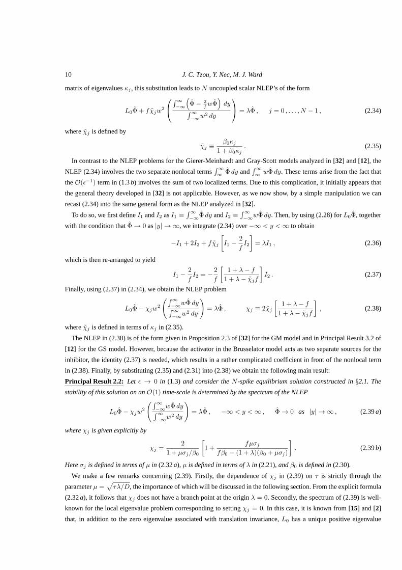
In Figure 3(a), we show a plot ofτ0j(D) for a three-spike example withf = 0.6. We again plot only the interval
0 < D < Dc3 above which thej = 2 curve ceases to exist. In the plot ofλ0Ij(D) in Figure 3(c), we see thatλ0I2 → 0
asD → D−
c3. In Figure 3(b), the reverse ordering principle is again observed for an interval ofD, indicating the
possibility of asynchronous oscillations. As similar to the previous two-spike case, forD to the right of this interval,
the usual ordering principle guaranteeing synchronous oscillatory instabilities is restored. The same characteristics of
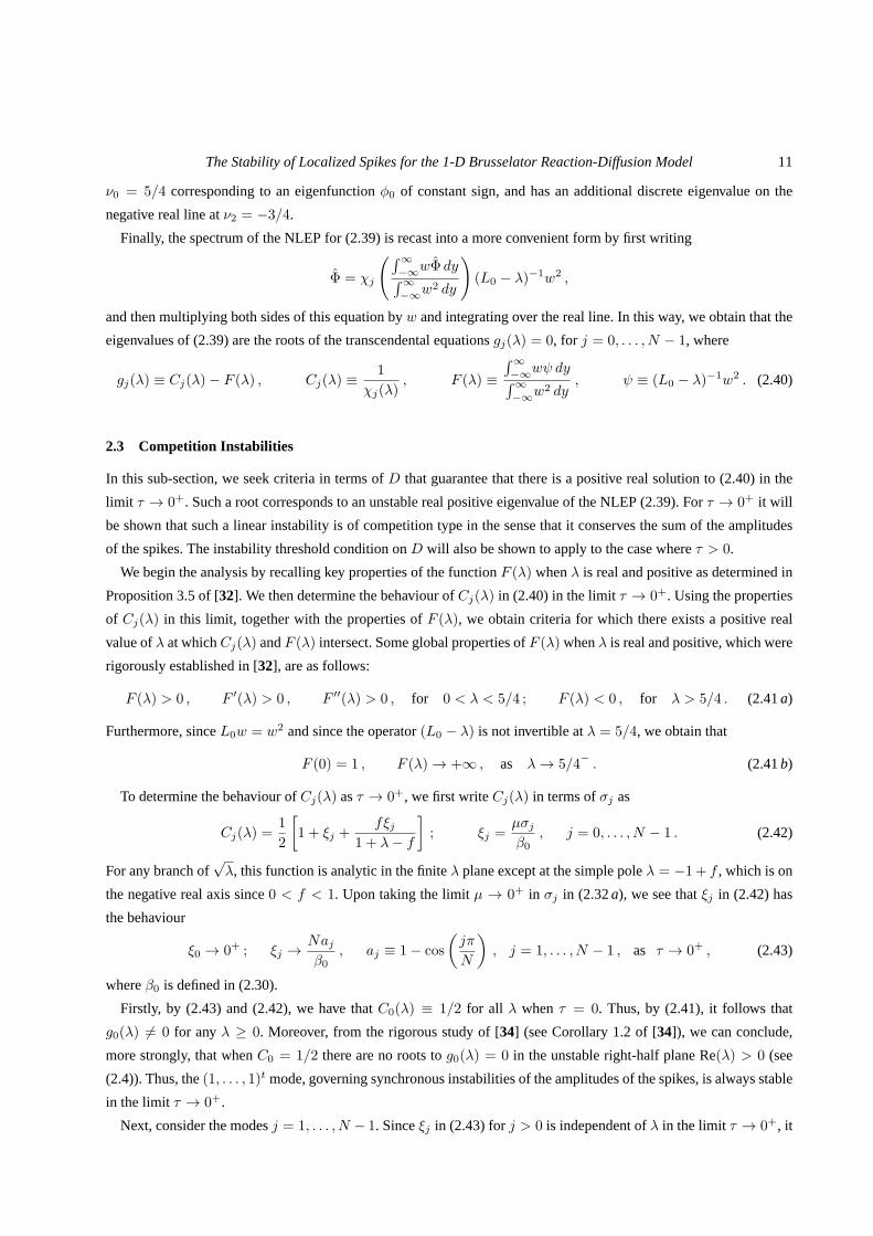
τ0j(D) andλ0Ij(D) for a four-spike example withf = 0.6 are seen in Figures 4(a)-4(c).
For the two-spike example of Figure 2 withf = 0.5, we trace the paths of the pair of complex conjugate eigenvalues
in the right-half plane asτ increases past the Hopf bifurcation value computed in Figures 2(a) and 2(b). For the two
modesj = 0 (Figure 5(a)) andj = 1 (Figure 5(b)), we start with the pair(τ, λ) = (τ0j(D), λ0Ij) and solveg(λ) = 0
in (2.40) for increasingly larger values ofτ . For thej = 0 mode we takeD = 0.03 while for thej = 1 mode, we take
D = 0.006 so that in both cases the eigenvalues being tracked are the first ones to cross into the right-half plane. The
eigenvalues converge onto the positive real axis whenτ is sufficiently large. Asτ is increased further, the eigenvalues
split and migrate along the positive axis toward0 andν0 = 5/4 asτ → ∞, whereν0 is the principal eigenvalue of the
operatorL0.
Two key characteristics shared by Figures 2-4 are the behaviours ofτ0j andλ0Ij for small values ofD. These figures
The Stability of Localized Spikes for the 1-D Brusselator Reaction-Diffusion Model 17
0 0.005 0.01 0.0150
0.5
1
1.5
2
2.5
3
3.5
4
D
τ 0j(D
)
(a) τ0j(D) for N = 3
2.6 2.8 3 3.2 3.4 3.6 3.8 4 4.2
x 10−3
1.2
1.3
1.4
1.5
1.6
1.7
1.8
1.9
2
2.1
Dτ 0
j(D
)
(b) τ0j(D) for N = 3 closeup
0 0.005 0.01 0.0150
0.1
0.2
0.3
0.4
0.5
0.6
0.7
D
λ0 Ij(D
)
(c) λ0
Ij(D) for N = 3
Figure 3. Plots ofτ0j(D) (left and center figures) andλ0Ij(D) (right figure) forN = 3 andf = 0.6. The critical value
Dc3 ≈ 0.0148 is indicated by the vertical dotted line. In all figures, the solid, dashed, and dotted curves correspond to
j = 0, 1, 2, respectively. In the magnified interval shown in the centerfigure,τ02 < τ01 < τ00.
0 1 2 3 4 5 6
x 10−3
0
0.5
1
1.5
2
2.5
3
3.5
4
D
τ 0j(D
)
(a) τ0j(D) for N = 4
1.1 1.2 1.3 1.4 1.5 1.6 1.7
x 10−3
0.9
1
1.1
1.2
1.3
1.4
1.5
1.6
D
τ 0j(D
)
(b) τ0j(D) for N = 4 closeup
0 1 2 3 4 5 6
x 10−3
0
0.1
0.2
0.3
0.4
0.5
D
λ0 Ij(D
)
(c) λ0
Ij(D) for N = 4
Figure 4. Plots ofτ0j(D) (left and center figures) andλ0Ij(D) (right figure) forN = 4 andf = 0.6. The critical value
Dc4 ≈ 0.0055 is indicated by the vertical dotted line. In all figures, the solid, dashed, dotted, and dash-dotted curves
correspond toj = 0, 1, 2, 3, respectively. In the magnified interval shown in the centerfigure,τ03 < τ02 < τ01 < τ00.
suggest thatτ0j → ∞ asD → 0 independent ofj, while λ0Ij approaches a constant value also independent ofj. We
now provide a simple analytical explanation for this limiting behaviour. We remark that this unbounded behaviour of
τ0j asD → 0 is in marked contrast to the finite limiting behaviour as obtained in [12] or [32] for the Gray-Scott and
Gierer-Meinhardt RD models, respectively.
In the limitD → 0, a simple scaling argument shows that|µ| → ∞, whereµ =√
τλ/D. We then readily obtain
from (2.32a) thatσj → 2 asD → 0 and thatβ0 = O(D−1). Therefore, from (2.42), we get the limiting behaviour
Cj ∼ C ≡ 1
2
[
1 + αz√λ+
αfz√λ
1− f + λ
]
, z =√τD, α =
α2v2c3
, j = 0, . . . , N − 1 . (2.58)
We setλ = iλI , whereλI > 0, and then separate (2.58) into real and imaginary parts to get
C ≡ CR(λI) + iCI(λI) ≡1
2
[
1 +αz√2
√
λIM+
]
+ i1
2√2αz√
λIM− ; M± ≡ 1− f ± λIf + λ2I(1− f)2 + λ2I
. (2.59)
SinceC is independent ofj, it follows that the rootτ = τ0l andλI = λIl to the limiting coupled systemCR(λI) =
FR(λI) andCI(λI) = FI(λI) must be independent ofj.
For this coupled system to possess a root, it is readily seen that we must havez =√τD = O(1) asD → 0, which

18 J. C. Tzou, Y. Nec, M. J. Ward
0 0.2 0.4 0.6 0.8 1 1.2−0.8
−0.6
−0.4
−0.2
0
0.2
0.4
0.6
0.8
λR
λI
(a) D = 0.03, j = 0
0 0.2 0.4 0.6 0.8 1 1.2−0.4
−0.3
−0.2
−0.1
0
0.1
0.2
0.3
0.4
λR
λI
(b) D = 0.006, j = 1
Figure 5. Plots of the paths ofλ = λI + iλR with N = 2, andf = 0.5 for (D, j) = (0.03, 0) (left) and(D, j) =
(0.006, 1) (right) asτ increases past its Hopf bifurcation valueτ0j(D). The arrows denote the direction of traversal for
increasingτ . The eigenvalues converge onto the positive real axis whenτ reaches some valueτc(D) > τ0j(D). The
eigenvalues split, with one tending to0 and the other tending toν0 = 5/4 asτ → ∞, whereν0 is the unique positive
eigenvalue of the operatorL0.
implies thatτ0l = O(D−1) asD → 0. We use (2.59) to eliminatez between the coupled systemCR(λI) = FR(λI)
andCI(λI) = FI(λI). In this way, we obtain thatλIl must be a root of
HR(λI) = HI(λI) , (2.60a)
whereHR(λI) andHI(λI) are defined by
HR(λI) =2FR(λI)− 1
λ2I + fλI + 1− f, HI =
2FI(λI)
λ2I − fλI + 1− f. (2.60b)
Therefore, forD → 0, we conclude thatλIl depends only onf and is independent ofN . The scalingτ0l = O(D−1)
was not observed in the analysis of the Gray-Scott [12] or Gierer-Meinhardt models [32].
We now prove the existence of a solutionλIl > 0 to (2.60). We begin by noting thatHR(0) = (1−f)−1 > 0 and that
HR(λI) has no poles whenλI ≥ 0. Also, becauseFR → 0 asλI → ∞, we find from (2.60b) thatHR ∼ −1/λ2I < 0
asλI → ∞. To show the existence of an intersection betweenHR andHI , there are two cases to consider. The first
case is when0 < f < 2(√2−1) so that the denominator ofHI is always positive. SinceFI(0) = 0 < FR(0) = 1, and
FI(λI) > 0 for λI > 0, then by the properties ofHR there must exist a solution to (2.60a). When2(√2−1) < f < 1,
HI(λI) has two poles on the positive real axis atλI = λl,rI ordered0 < λlI < λrI with λlI → 0+ asf → 1−. Therefore,
HI → +∞ asλI → λl−I . BecauseHR(0) > 0 and is bounded for allλI whileHI(0) = 0, there must exist a solution
to (2.60a) on the interval0 < λI < λlI . This completes the proof of the existence of a rootλIl > 0 under the scaling
τ = O(D−1) asD → 0. While we have not been able to show analytically thatλIl is unique, we have not observed
numerically an example that yields more than one solution to(2.60a).
In Figure 6(a), we show the log-log relationship betweenτ0j and smallD for the examples shown in Figures 2 - 4.
Note that in each case, all curves corresponding to modesj = 0, . . . , N − 1 are plotted. However, as stated above,
τ0j is independent ofj for smallD and thus the curves are indistinguishable in the plot. In Figure 6(b), we plot theN

The Stability of Localized Spikes for the 1-D Brusselator Reaction-Diffusion Model 19
curves ofλ0Ij as a function off with D small forN = 2, 3, 4. We also plot the solution to (2.60a). Although for each
value ofN we use a different value ofD specified asD = DcN/10, all curves are indistinguishable at the resolution
allowed by the figure. BecauseλlI → 0+ asf → 1−, we expect theoretically thatλIl → 0+ in this limit. Numerically,
however, the problem (2.60a) for 1 − f small becomes ill-conditioned and our numerical solver fails whenf is too
close tof = 1.
10−5
10−4
10−3
10−2
10−1
100
101
102
103
D
z
(a) log-log plot of τ0j(D) for N = 2, 3, 4 andD ≪ 1
0 0.2 0.4 0.6 0.8 10
0.1
0.2
0.3
0.4
0.5
f
λ0 Ij
(b) λ0
Ij versusf for N = 2, 3, 4 andD ≪ 1
Figure 6. The log-log relationship betweenτ0j and smallD with parameters from Figures 2 - 4 (left) andλ0Ij versus
f with D small forN = 2, 3, 4 (right). In the left figure, the solid lines are numerically computed solutions ofgRj =
gIj = 0, while the dotted lines all have slope−1. The top line corresponds toN = 2, f = 0.5, the center line to
N = 3, f = 0.6, and the bottom line toN = 4 andf = 0.6. The different curves of each example corresponding to
modesj = 0, . . . , N − 1 are indistinguishable. In the right figure, the curves ofλ0Ij versusf generated by the solution
to gRj = gIj = 0 are plotted, as is the solution to (2.60a). These curves are indistinguishable at the resolution allowed
by the figure.
The main limitation of our analysis is that we are unable to determine whether, for each functiongj , a complex
conjugate pair of pure imaginary eigenvalues exists at onlyone value ofτ0j for all the ranges of the parameters. Our
numerical experiments suggest that for0 < τ < τ0j andD < D0cN , the pattern is stable. This indicates that our
computed thresholdsτ0j are the minimum values ofτ for which an oscillatory instability occurs.
One possible way to obtain a rigorous bound onτ0j is to use the following inequality, as derived in equation (2.29)
of [33] (see also equation (5.62) of [35]), for any eigenvalueλ of the NLEP of (2.39) with multiplierχj :
|χj − 1|2 + Re(
λχj
)
(∫∞
−∞w2 dy
∫∞
−∞w3 dy
)
≤ 0 . (2.61)
Upon evaluating the integral ratio, and then usingχj = 1/Cj and Re(z) = Re(z), we obtain that (2.61) reduces to
|Cj − 1|2 + 5
6Re(λCj) ≤ 0 . (2.62)
For the reaction-diffusion systems in [33] and§5 of [35] for which Cj is a simple rational function ofλ, (2.62) was
used successfully to obtain a rigorous bound on the Hopf bifurcation threshold ofτ . However, for the Brusselator,Cj
20 J. C. Tzou, Y. Nec, M. J. Ward
in (2.42) is not rational inλ, and it is not clear how to use (2.62) to obtain an explicit analytical bound on the Hopf
bifurcation thresholdτ0j .
2.5 Numerical Validation
Next, we illustrate the theory presented in§2.3 and§2.4 regarding competition and oscillatory instabilities of N -
spike equilibria. We solve the Brusselator model without boundary flux (1.3) numerically using theMATLAB partial
differential equations solverpdepe() with non-uniformly spaced grid points distributed according to the mapping
y = x+
N−1∑
i=0
tanh
[
x− xi2ǫ
]
; −1−N < y < 1 +N,
wherex is the physical grid. The initial conditions were taken to bea perturbation of the equilibrium spike solution of
the form
u(x, 0) = u∗e(x)
[
1 + δ
N−1∑
k=0
dke−(x−xk)
2/(4ǫ2)
]
, v(x, 0) = v∗e(x), (2.63)
whereδ ≪ 1 is taken to be0.002, anddk is the(k + 1)th component of the vectord to be defined below. Either2000
(ǫ = 0.005) or 4000 (ǫ = 0.001) grid points were used to produce the numerical results below. In (2.63), instead of
ue, ve given in (2.15), we use the true equilibriumu∗e, v∗e calculated using smallτ starting from the initial conditions
ue, ve. Becauseτ does not influence the equilibrium solution,u∗e, v∗e may be used as valid initial conditions for any
value ofτ . We briefly explain the reason for this procedure. With an insufficiently small choice forτ while starting
with ue andve as initial conditions, we observe an immediate annihilation of one or more of the spikes. We conjecture
that this is due to the inaccuracy of the asymptotic solutionassociated with the non-zero background of the activator,
coupled with the sluggish response of the inhibitor. However, for τ sufficiently small, the inhibitor is able to respond
quickly to prevent an annihilation, allowing the system to evolve to a spike equilibrium stateu∗e, v∗e .
In (2.63), the choice of the vectord depends on the phenomenon that we illustrate. In computations illustrating
competition instabilities,d is taken to be a multiple ofvN−1, the eigenvector given in (2.32c) associated with the
eigenvalue that first crosses into the right-half plane asD is increased aboveDcN whenτ is sufficiently small. The
values ofD in the experiments illustrating competition instabilities will be such that only thej = N − 1 mode is
unstable. In computations illustrating oscillatory instabilities,d is taken to be a multiple of the vector∑N−1
j=0 vj , with
vj given in (2.32c), which allows for all the modes to be present initially. We track the evolution of the modes through
the quantitybampj , defined as the amplitude of the oscillations ofbj given by
bj = |∆utmvj | , ∆um ≡ (um0 − u∗e(x0, 0) , . . . , umN−1 − u∗e(xN−1, 0))
t ; j = 0, . . . , N − 1 , (2.64)
allowing clear identification of which modes grow or decay. Hereumn denotes the numerically computed solution at
thejth equilibrium spike location defined byumj ≡ u(xj , t) wherexj = −1 + (2j + 1)/N with j = 0, . . . , N − 1.
In all experiments,d is normalized so thatmaxk dk = 1.
We consider three experiments with two, three, and four spikes. In each experiment,f is fixed while different
combinations ofτ andD are used to illustrate the theory for competition and oscillatory instabilities. The results are
presented using plots of the amplitude of each spikeumn ≡ u(xn, t) versus time. For certain oscillatory examples, we

The Stability of Localized Spikes for the 1-D Brusselator Reaction-Diffusion Model 21
also plot the quantitybampj versus time. In our computations, we limit the time-scale tomuch less thanO(ǫ−2) so that
the spikes remain approximately stationary over the time intervals shown.
Experiment 1: In this experiment we consider competition and oscillatoryinstabilities of a two-spike equilibrium
with f = 0.5. We begin with an example of competition instability. Forǫ = 0.005 andD = 0.043, in Figure 7(a) we
plot the initial conditions foru andv on the left and right axes, respectively. Note the non-zero background ofu. Using
the results depicted in Figure 2(a), we calculate thatτ0(D) = 0.165, while using (2.45) we calculateDc2 = 0.0417.
For τ = 0.01 < τ0(D) andD > Dc2, we expect a competition instability in which one spike is annihilated with
no oscillation in the amplitudes. In Figure 7(b), we plot theamplitudesum0 andum1 of the two spikes as a function
of time. As suggested by the eigenvectorv1 in (2.32c), one spike annihilates as time increases. Note that the spike
amplitude decays to approximately the value of the non-zerobackground state.
−1 −0.5 0 0.5 10
0.1
0.2
0.3
x
ue
−1 −0.5 0 0.5 112
13
14
15v e
(a) initial condition foru andv
0 50 100 150 2000
0.05
0.1
0.15
0.2
0.25
0.3
0.35
0.4
0.45
0.5
t
um
(b) um versust
Figure 7. Experiment 1: The left figure is the initial condition foru (solid curve and left axis) andv (dashed curve and
right axis) forN = 2 with ǫ = 0.005, f = 0.5 andD = 0.043 > Dc2 = 0.0417. The right figure shows the amplitudes
of the left (solid curve) and right (dashed curve) spikes forτ = 0.01 versus time. The right spike annihilates as time
increases.
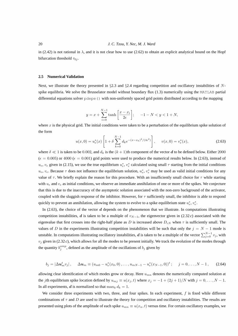
We now illustrate oscillatory phenomena. In Figure 8(a), weplot the spike amplitudes whenD = 0.03 < Dc2
andτ = 0.17 < τ0(D) = τ00 = 0.183. As expected, no spike annihilations occur while initial oscillations decay.
While the equilibrium is stable to large eigenvalues for thiscombination ofD andτ , we calculate from (2.47) that
D > D∗2 = 0.021. Thus, we expect to observe a drift-type instability whent = O(ǫ−2). Next, for the same value of
D, we setτ = 0.191 > τ0(D) so that the synchronous mode undergoes a Hopf bifurcation. The spike amplitudes are
plotted in Figure 8(b). As expected, the spike amplitudes synchronize quickly and oscillate with growing amplitude
in time. The eventual annihilation of the spikes suggests that the Hopf bifurcation is subcritical for these parameter
values.
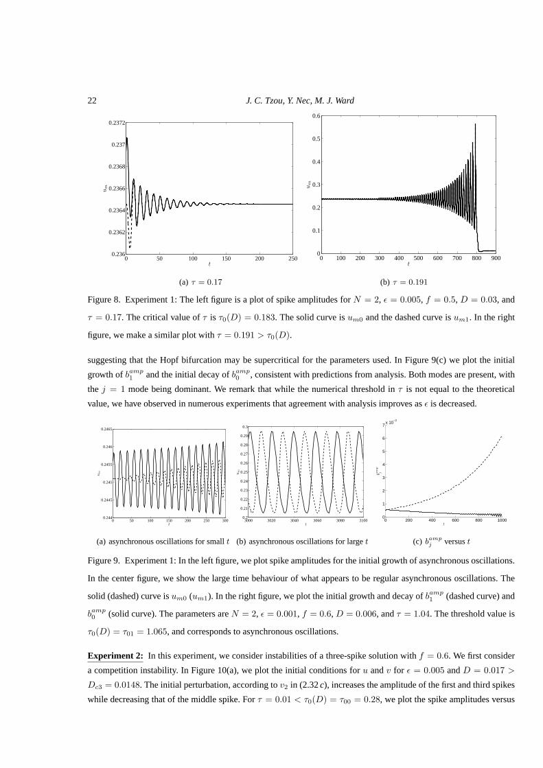
In the next example, we takeǫ = 0.001 andD = 0.006. In Figure 2(b) we see that for this value ofD, the
asynchronous oscillatory mode is unstable ifτ > τ0(D) = τ01 = 1.065 while the synchronous mode is stable if
τ < τ00 = 1.083. In Figure 9(a), we plot the spike amplitudes whenτ = 1.04 during the initial growth of the
oscillations. Note the clear contrast between Figure 9(a) and Figure 8(b) where the spikes oscillate out of phase in
the former and in phase in the latter. In Figure 9(b), we show what appears to be regular asynchronous oscillations,
22 J. C. Tzou, Y. Nec, M. J. Ward
0 50 100 150 200 2500.236
0.2362
0.2364
0.2366
0.2368
0.237
0.2372
t
um
(a) τ = 0.17
0 100 200 300 400 500 600 700 800 9000
0.1
0.2
0.3
0.4
0.5
0.6
t
um
(b) τ = 0.191
Figure 8. Experiment 1: The left figure is a plot of spike amplitudes forN = 2, ǫ = 0.005, f = 0.5, D = 0.03, and
τ = 0.17. The critical value ofτ is τ0(D) = 0.183. The solid curve isum0 and the dashed curve isum1. In the right
figure, we make a similar plot withτ = 0.191 > τ0(D).
suggesting that the Hopf bifurcation may be supercritical for the parameters used. In Figure 9(c) we plot the initial
growth ofbamp1 and the initial decay ofbamp
0 , consistent with predictions from analysis. Both modes arepresent, with
the j = 1 mode being dominant. We remark that while the numerical threshold inτ is not equal to the theoretical
value, we have observed in numerous experiments that agreement with analysis improves asǫ is decreased.
0 50 100 150 200 250 3000.244
0.2445
0.245
0.2455
0.246
0.2465
t
um
(a) asynchronous oscillations for smallt
3000 3020 3040 3060 3080 31000.2
0.21
0.22
0.23
0.24
0.25
0.26
0.27
0.28
0.29
0.3
t
um
(b) asynchronous oscillations for larget
0 200 400 600 800 10000
1
2
3
4
5
6
7x 10
−3
t
bam
pj
(c) bamp
j versust
Figure 9. Experiment 1: In the left figure, we plot spike amplitudes for the initial growth of asynchronous oscillations.
In the center figure, we show the large time behaviour of what appears to be regular asynchronous oscillations. The
solid (dashed) curve isum0 (um1). In the right figure, we plot the initial growth and decay ofbamp1 (dashed curve) and
bamp0 (solid curve). The parameters areN = 2, ǫ = 0.001, f = 0.6,D = 0.006, andτ = 1.04. The threshold value is
τ0(D) = τ01 = 1.065, and corresponds to asynchronous oscillations.
Experiment 2: In this experiment, we consider instabilities of a three-spike solution withf = 0.6. We first consider
a competition instability. In Figure 10(a), we plot the initial conditions foru andv for ǫ = 0.005 andD = 0.017 >
Dc3 = 0.0148. The initial perturbation, according tov2 in (2.32c), increases the amplitude of the first and third spikes
while decreasing that of the middle spike. Forτ = 0.01 < τ0(D) = τ00 = 0.28, we plot the spike amplitudes versus

The Stability of Localized Spikes for the 1-D Brusselator Reaction-Diffusion Model 23
time in Figure 10(b), observing that the middle spike annihilates while the other two spikes increase in amplitude. This
increase in amplitude, also observed in Figure 7(b) of Experiment 1, is expected because the common spike amplitude
increases when the number of spikes decreases (see (2.8) and(2.15a)). For a perturbation in the−v2 direction we
observe the annihilation of the first and third spikes (not shown).
−1 −0.5 0 0.5 10
0.05
0.1
0.15
0.2
0.25
x
ue
−1 −0.5 0 0.5 19
10
11
12
13
14
v e
(a) initial conditions foru andv
0 20 40 60 80 100 1200
0.05
0.1
0.15
0.2
0.25
0.3
0.35
0.4
t
um
(b) um versust
Figure 10. Experiment 2: The left figure is the initial condition for u (solid curve and left axis) andv (dashed curve
and right axis) forN = 3 with ǫ = 0.005, f = 0.6, andD = 0.017 > Dc3 = 0.0148. In the right figure, we plot
um0 andum2 (solid curve) andum1 (dashed curve) versus time withτ = 0.01. The second spike annihilates as time
increases.
To illustrate oscillatory behaviour, we takeǫ = 0.005 andD = 0.009 so that all real eigenvalues lie in the left-
half plane if τ is small enough. Using Figure 3(a), we calculateτ0(D) = τ00 = 0.3994. In Figure 11(a), we set
τ = 0.37 < τ0(D) so that oscillations decay in time. For stability also to small eigenvalues, however, we require
D < D∗3 = 0.011. In Figure 11(b), we setτ = 0.42 so that the spike amplitudes quickly synchronize and the
subsequent oscillations grow in time. As in Experiment 1, weobserve the annihilation of the spikes, suggesting that
the Hopf bifurcation is subcritical.
We next decreaseD toD = 0.0034 so that, as suggested by Figure 3(b), asynchronous oscillations are the dominant
instability. We calculate thatτ0(D) = τ02 = 1.518, τ01 = 1.544, andτ00 = 1.557. In Figures 12(a) and 12(b) we
plot, respectively, the transient and large time behaviourof the spike amplitudes forǫ = 0.001 andτ = 1.51. In clear
contrast to Figure 11(b), the spike amplitudes oscillate out of phase for both small and large time. In Figure 12(b), as
the form of the eigenvectorv2 in (2.32c) suggests, the first and third spikes oscillate approximately in phase with each
other while out of phase with the second spike. For large time, the oscillations occur within an envelope that oscillates
slowly in time relative to the oscillations of the spike amplitudes. In Figure 12(c), we plot the initial growth and decay
of bampj for all three modes. Consistent with the results depicted inFigure 3(b), thej = 2 mode grows while the other
two modes decay. For large time, all modes are present with the dominant mode beingj = 2.
Experiment 3: In this experiment, we illustrate instabilities of a four-spike equilibrium withf = 0.6. In Figure
13(a), we plot the initial conditions foru andv with ǫ = 0.005 andD = 0.0057. We calculate from (2.45) that
Dc4 = 0.0055 < D. With τ = 0.01 < τ0(D) = 0.2344, we expect an annihilation of one or more spikes without
oscillatory behaviour. The form ofv3 in (2.32c) suggests that the second spike is the first to annihilate while the fourth

24 J. C. Tzou, Y. Nec, M. J. Ward
0 50 100 150 200 2500.2362
0.2363
0.2364
0.2365
0.2366
0.2367
0.2368
0.2369
0.237
0.2371
0.2372
t
um
(a) τ = 0.37
0 100 200 300 400 500 600 7000
0.05
0.1
0.15
0.2
0.25
0.3
0.35
0.4
0.45
t
um
(b) τ = 0.42
Figure 11. Experiment 2: In the left figure, we plotum0 (solid curve),um1 (dashed curve), andum2 (dotted curve)
for N = 3, ǫ = 0.005, f = 0.6, D = 0.009, andτ = 0.37. The right figure is similar except thatτ is increased to
τ = 0.42. The critical value ofτ is τ0(D) = 0.3994.
0 50 100 150 2000.2445
0.245
0.2455
0.246
0.2465
0.247
t
um
(a) asynchronous oscillations for smallt
3000 3020 3040 3060 3080 31000.2
0.21
0.22
0.23
0.24
0.25
0.26
0.27
0.28
0.29
0.3
t
um
(b) asynchronous oscillations for larget
0 200 400 600 800 10000
0.5
1
1.5
2
2.5
3
3.5
4
x 10−3
t
bam
pj
(c) bamp
j versust
Figure 12. Experiment 2: In the left and center figures, we plot, respectively, the transient and large time asynchronous
oscillations ofum0 (solid curve),um1 (dashed curve), andum2 (dotted curve). The first and third spikes oscillate almost
in phase for large time. In the right figure, we plot the initial growth and decay ofbampj for j = 0 (solid curve),j = 1
(dashed curve), andj = 2 (dotted curve). The parameters areN = 3, ǫ = 0.001, f = 0.6,D = 0.0034, andτ = 1.51.
The threshold value isτ0(D) = τ02 = 1.518.
spike decays in amplitude as the other two spikes grow. Once the first annihilation occurs, the resulting three-spike
pattern is no longer in equilibrium and thus evolves according to the dynamics derived in [27], and any subsequent
annihilations should they occur are beyond the scope of thisanalysis. In Figure 13(b), we plot the spike amplitudes up
to the time of the annihilation of the second spike.
To show oscillatory phenomena, we takeǫ = 0.005 andD = 0.004. Using the data from Figure 4(a), we calculate
τ0(D) = τ00 = 0.287. In Figure 14(a), we plot the spike amplitudes forτ = 0.27 so that the equilibrium solution
is stable to large eigenvalues. Here, we requireD < D∗4 = 0.00469 for the equilibrium to also be stable to small

The Stability of Localized Spikes for the 1-D Brusselator Reaction-Diffusion Model 25
−1 −0.5 0 0.5 10
0.05
0.1
0.15
0.2
x
ue
−1 −0.5 0 0.5 112
14
16
18
20
v e
(a) initial conditions foru andv
0 50 100 150 200 250 3000
0.05
0.1
0.15
0.2
0.25
t
um
(b) um versust
Figure 13. Experiment 3: The left figure is the initial condition for u (solid curve and left axis) andv (dashed curve
and right axis) forN = 4 with ǫ = 0.005, f = 0.6, andD = 0.0057 > Dc4 = 0.0055. In the right figure, we plot
um0 (solid curve),um1 (dashed curve),um2 (dotted curve), andum3 (dash-dotted) curve versus time withτ = 0.01.
The second spike annihilates as time increases. All complexeigenvalues are in the stable left-half plane.
eigenvalues. In Figure 14(b), we plot the spike amplitudes for τ = 0.31 so that synchronous oscillations grow in time
until all spikes annihilate. As in Experiment 2, we observe oscillatory behaviour subsequent to annihilation.
0 50 100 150 200 2500.1738
0.1739
0.174
0.1741
0.1742
0.1743
0.1744
0.1745
0.1746
t
um
(a) τ = 0.27
0 100 200 300 400 5000
0.05
0.1
0.15
0.2
0.25
0.3
0.35
0.4
t
um
(b) τ = 0.31
Figure 14. Experiment 3: In the left figure, we plotum0 (solid curve),um1 (dashed curve), andum2 (dotted curve)
andum3 (dash-dotted curve) forN = 4, ǫ = 0.005, f = 0.6, D = 0.004, andτ = 0.27. The right figure is similar
exceptτ = 0.31. The critical value ofτ is τ0(D) ≈ 0.287.
Lastly, we illustrate asynchronous oscillations withǫ = 0.001 andD = 0.0015. According to the data in Figure
4(b), we calculate thatτ0(D) = τ03 = 1.084, τ02 = 1.098, τ01 = 1.112, andτ00 = 1.118. Takingτ = 1.06, we plot
the initial growth of asynchronous oscillations in Figure 15(a). The form ofv3 suggests that the first and fourth spikes
oscillateπ radians out of phase as should the second and third spikes, while no spikes oscillate in phase. This is shown
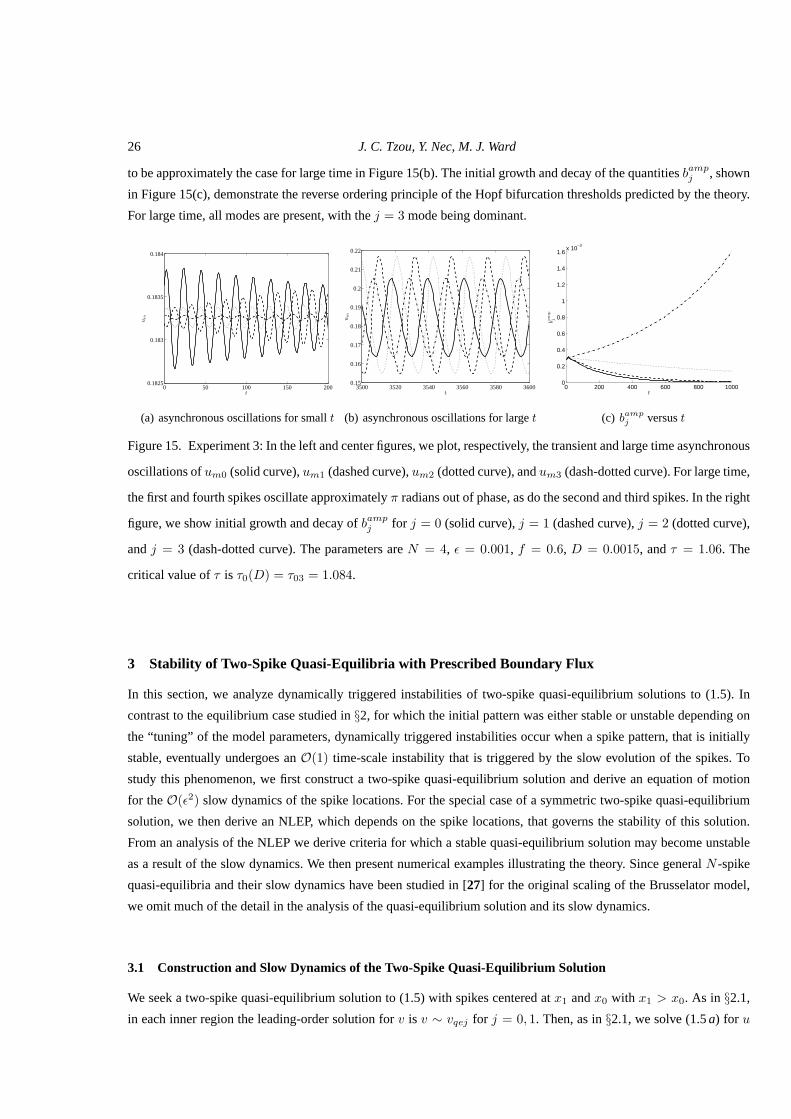
26 J. C. Tzou, Y. Nec, M. J. Ward
to be approximately the case for large time in Figure 15(b). The initial growth and decay of the quantitiesbampj , shown
in Figure 15(c), demonstrate the reverse ordering principle of the Hopf bifurcation thresholds predicted by the theory.
For large time, all modes are present, with thej = 3 mode being dominant.
0 50 100 150 2000.1825
0.183
0.1835
0.184
t
um
(a) asynchronous oscillations for smallt
3500 3520 3540 3560 3580 36000.15
0.16
0.17
0.18
0.19
0.2
0.21
0.22
t
um
(b) asynchronous oscillations for larget
0 200 400 600 800 10000
0.2
0.4
0.6
0.8
1
1.2
1.4
1.6x 10
−3
t
bam
pj
(c) bamp
j versust
Figure 15. Experiment 3: In the left and center figures, we plot, respectively, the transient and large time asynchronous
oscillations ofum0 (solid curve),um1 (dashed curve),um2 (dotted curve), andum3 (dash-dotted curve). For large time,
the first and fourth spikes oscillate approximatelyπ radians out of phase, as do the second and third spikes. In theright
figure, we show initial growth and decay ofbampj for j = 0 (solid curve),j = 1 (dashed curve),j = 2 (dotted curve),
andj = 3 (dash-dotted curve). The parameters areN = 4, ǫ = 0.001, f = 0.6, D = 0.0015, andτ = 1.06. The
critical value ofτ is τ0(D) = τ03 = 1.084.
3 Stability of Two-Spike Quasi-Equilibria with Prescribed Boundary Flux
In this section, we analyze dynamically triggered instabilities of two-spike quasi-equilibrium solutions to (1.5). In
contrast to the equilibrium case studied in§2, for which the initial pattern was either stable or unstable depending on
the “tuning” of the model parameters, dynamically triggered instabilities occur when a spike pattern, that is initially
stable, eventually undergoes anO(1) time-scale instability that is triggered by the slow evolution of the spikes. To
study this phenomenon, we first construct a two-spike quasi-equilibrium solution and derive an equation of motion
for theO(ǫ2) slow dynamics of the spike locations. For the special case ofa symmetric two-spike quasi-equilibrium
solution, we then derive an NLEP, which depends on the spike locations, that governs the stability of this solution.
From an analysis of the NLEP we derive criteria for which a stable quasi-equilibrium solution may become unstable
as a result of the slow dynamics. We then present numerical examples illustrating the theory. Since generalN -spike
quasi-equilibria and their slow dynamics have been studiedin [27] for the original scaling of the Brusselator model,
we omit much of the detail in the analysis of the quasi-equilibrium solution and its slow dynamics.
3.1 Construction and Slow Dynamics of the Two-Spike Quasi-Equilibrium Solution
We seek a two-spike quasi-equilibrium solution to (1.5) with spikes centered atx1 andx0 with x1 > x0. As in §2.1,
in each inner region the leading-order solution forv is v ∼ vqej for j = 0, 1. Then, as in§2.1, we solve (1.5a) for u

The Stability of Localized Spikes for the 1-D Brusselator Reaction-Diffusion Model 27
in the inner region of thejth spike to get
u ∼ 1
fvqejw(yj) , yj = ǫ−1(x− xj) , for j = 0, 1 ,
wherew(y) is the solution to (2.2). In the outer regionu ∼ ǫE +O(ǫ2). Then, upon representing the terms involving
u in (1.5b) as delta masses, we proceed as in§2.1 and use (2.3) to obtain that the outer equation forv is
Dvxx + E − 6
f2(1− f)
1∑
j=0
δ(x− xj)
vqej= 0 , −1 < x < 1 ; vx(±1) = ±1 . (3.1)
Upon integrating (3.1) over the interval−1 < x < 1 and applying the boundary conditions, we calculate that
1∑
j=0
1
vqej=
(E +D)
3
f2
1− f> 0 . (3.2)
For the special case of a symmetric two-spike quasi-equilibrium wherex1 = −x0 = α, thenvqe0 = vqe1 ≡ vcqe,
wherevcqe is given by
vcqe =6
f2(D + E)(1− f) > 0 . (3.3)
Note that due to the presence of boundary flux, the spike amplitudes depend on the inhibitor diffusion coefficient.
Next, we letv = x2/2+ ν(x) and solve forν(x) in terms ofG, as defined in (2.13). Then, we impose the matching
condition thatv(xj) = vqej for j = 0, 1. In this way, we obtain the following result for the quasi-equilibrium solution:
Principal Result 3.1: Let ǫ→ 0 in (1.5)and consider a two-spike quasi-equilibrium solution with spikes centered at
x1 andx0 with x1 > x0. Then, the leading order composite solution foru is
uqe ∼ ǫE +1
fvqe0w[
ǫ−1(x− x0)]
+1
fvqe1w[
ǫ−1(x− x1)]
, (3.4a)
while the leading order outer solutionvqe for v is given by
vqe ∼ ν +x2
2+
6
f2(1− f)
1∑
j=0
1
vqejG(x;xj) , (3.4b)
whereG is the Green’s function defined in(2.13). Herevqe0, vqe1, andν satisfy the coupled system consisting of (3.2)
and
vqe0 = ν +x202
+6
f2(1− f)
(
G(x0;x0)
vqe0+G(x0;x1)
vqe1
)
, (3.5a)
vqe1 = ν +x212
+6
f2(1− f)
(
G(x1;x0)
vqe0+G(x1;x1)
vqe1
)
. (3.5b)
By subtracting the two equations in (3.5), and then using (2.13) forG, we obtain thatvqe0 andvqe1 satisfy
vqe1 − vqe0 = a− b
(
1
vqe1− 1
vqe0
)
,1
vqe0+
1
vqe1= c , (3.6a)
where we have defineda, b, andc, by
a ≡ − E
2D(x21−x20) , b ≡ ζ0(x1−x0) > 0 , c ≡ 1
ζ0
(
1 +E
D
)
> 0 , ζ0 ≡ 3
Df2(1− f) > 0 . (3.6b)
By eliminatingvqe0 in (3.6a), we readily derive that
vqe0 =ξ
c(ξ − 1), vqe1 =
ξ
c, (3.7a)

28 J. C. Tzou, Y. Nec, M. J. Ward
whereξ is a root of the cubic
K(ξ) ≡ (ξ − 2)(ξ2 − bc2ξ + bc2) + acξ(1− ξ) = 0 , (3.7b)
on the intervalξ > 1.
In discussing the solvability of (3.7) we will consider two cases: Case 1 wherex1 = −x0 and Case 2 wherex1 6= x0.
For Case I, suppose that the initial data is such thatx1 = −x0 at timet = 0. Sincea = 0, we obtain that (3.7b) has a
unique rootξ = 2 whenc < 2/√b, and it has three rootsξ = 2 andξ = ξ± > 1 whenc > 2/
√b, whereξ± is defined
by
ξ± =bc2
2
[
1±√
1− 4
bc2
]
, for c > 2/√b . (3.8)
Therefore, whenx1 = −x0, we have a symmetric two-spike quasi-equilibrium solutionwith vqe0 = vqe1 = 2/c, and
two asymmetric quasi-equilibrium solutions with eithervqe0 < vqe1 or vqe1 < vqe0 that exist whenc > 2/√b. These
asymmetric quasi-equilibria arise from a pitchfork bifurcation at the critical valuec = 2/√b.
Remark 1. From an analysis of an NLEP in§3.2 below (see equation (3.29)), we will show that the two asymmetric
quasi-equilibria forx1 = −x0 andc > 2/√b are unstable on anO(1) time-scale for anyτ ≥ 0.
Next, we briefly consider the generic Case II wherex1 6= x0 so thata 6= 0. Then, sinceK(1) = −1 < 0 and
K → +∞ asξ → +∞, there is always a root to (3.7b) on ξ > 1. Therefore, there always exists a two-spike quasi-
equilibrium state for anyx1 > x0. By plottingK(ξ) it readily follows that there is a unique root toK(ξ) = 0 when
|a| ≫ 1. For smaller values of|a| and whenbc2 > 4, there can be three quasi-equilibrium states. SinceK(ξ) is a cubic,
which therefore has at most two critical points, a sufficientcondition forK(ξ) = 0 to have a unique root onξ > 1 is
thatK′(1) < 0. This yields the inequalitybc2 − ac < 1.
Next, we derive theO(ǫ2) slow dynamics of the spike locations. We introduce the slow time variableσ = ǫ2t and
we retain the next terms in the asymptotic series for the inner solutions ofu andv nearxj as
u =1
fvqejw(yj) + ǫU1j(yj) , v = vqej + ǫV1j(yj) ; yj = ǫ−1 [x− xj(σ)] , σ = ǫ2t . (3.9)
Substituting (3.9) into (1.5), and collecting terms of similar orders, we obtain that
L0U1j = − xjfvqej
w′ − E − w2
fv2qejV1j , −∞ < yj <∞ , U ′
1j → 0 as |yj | → ∞ , (3.10a)
DV ′′
1j = − w
fvqej+
w2
f2vqej, −∞ < yj <∞ , V ′
1j → vqex(x±
j ) as yj → ±∞ , (3.10b)
wherexj ≡ dxj/dσ and the operatorL0 is defined in (2.28). The limiting condition in (3.10b) comes from matching
the gradients of the inner and outer solutions ofv. In (3.10a), L0 has a one-dimensional kernel with eigenfunctionw′.
Thus, the right-hand side of (3.10a) must be orthogonal tow′. This solvability condition yields
− xjfvqej
∫ ∞
−∞
(w′)2 dyj − E
∫ ∞
−∞
w′ dyj −1
fv2qej
∫ ∞
−∞
w′w2V1j dyj = 0 .
Sincew′ is odd andw′w2 = (w3)′/3, we can integrate by parts and usew → 0 as|yj | → ∞ to obtain
xj
∫ ∞
−∞
(w′)2 dyj =1
3vqej
∫ ∞
−∞
w3V ′
1j dyj . (3.11)
Next, we integrate by parts on the right-hand side of (3.11).Using the facts that∫ yj
0w3(s) ds is odd and that, by

The Stability of Localized Spikes for the 1-D Brusselator Reaction-Diffusion Model 29
(3.10b), V1j is even, we calculate that
xj
∫ ∞
−∞
(w′)2 dyj =1
6vqej
∫ ∞
−∞
w3 dyj[
V ′
1j(∞) + V ′
1j(−∞)]
. (3.12)
Finally, since∫
∞
−∞w3 dyj∫
∞
−∞(w′)2 dyj
= 6, we can apply the limiting conditions forV1j in (3.10b) to reduce (3.12) to
xj =1
vqej
[
vqex(x+j ) + vqex(x
−
j )]
. (3.13)
To calculate the right-hand side of (3.13), we use (3.4b) and (2.13). In this way, we obtain the following ODE-DAE
system characterizing the slow dynamics ofx0 andx1:
Principal Result 3.2: Consider the quasi-equilibrium solution(3.4) of (1.5) with spikes centered atx1 andx0 with
−1 < x0 < x1 < 1. Then, forǫ → 0, and provided that the quasi-equilibrium profile is stable to O(1) time-scale
instabilities, the spikes drift with speedO(ǫ2) according to the asymptotic ODE-DAE system
x0 ∼ 2
vqe0
[
x0 − ζ0
(
x0vqe0
+(1 + x0)
vqe1
)]
, x1 ∼ 2
vqe1
[
x1 + ζ0
(
(1− x1)
vqe0− x1vqe1
)]
. (3.14)
Herevqe0 andvqe1, which depend onx0 andx1, are positive solutions of the nonlinear algebraic system (3.6), while
ζ0 is defined in (3.6 b).
For the special case of a symmetric two-spike quasi-equilibrium solution withx1 = −x0 ≡ α andvqe1 = vqe0 =
vcqe, we use (3.3) to simplify (3.14). This leads to the followingresult:
Principal Result 3.3: Consider the quasi-equilibrium solution(3.4)of (1.5)with spikes centered atx1 = −x0 ≡ α
for 0 < α < 1, for which the spikes have a common amplitude, i.e.vqe0 = vqe1 = vcqe. Then, forǫ→ 0, and provided
that the quasi-equilibrium profile is stable toO(1) time-scale instabilities, the spikes drift with speedO(ǫ2) according
to the ODE
dα
dt∼ ǫ2H(α) ; H(α) ≡ 1
vcqe
[
1 +E
D− 2αE
D
]
. (3.15)
Herevcqe, which is independent of the spike locations, is defined in(3.3). The equilibrium locations of the spikes are
at ±αe whereH(αe) = 0, which yields
αe =1
2+
D
2E. (3.16)
Due to the imposed boundary flux, these equilibrium locations are not at the symmetry locations±1/2 of the no
boundary flux system studied previously in§2. From (3.16), we observe that for the equilibrium locations to be inside
the domain, we must have thatD/E < 1. SinceH′(αe) < 0, the equilibrium points of the ODE are always stable.
We limit our study to the parameter range where the inequality D/E < 1 is satisfied. We note that the symmetric
equilibrium is stable under the dynamics (3.15), which was derived under the assumption thatx0 = −x1. That is,
the equilibrium (3.16) is stable only to perturbations thatpreserve this symmetry. For the equilibrium to be stable to
any perturbation, including to those that break the symmetry, the parametersD, E andf must satisfy the condition
(cf. [27])
1− f
Ef2<
1
24
E
D
[
1 +D
E
]3
. (3.17)
The criterion (3.17), as derived in [27], is the condition that must be satisfied for a two-spike symmetric equilibrium
solution to be stable to eigenvalues ofO(ǫ2).

30 J. C. Tzou, Y. Nec, M. J. Ward
3.2 Derivation of the NLEP
In this subsection, we study the stability of the two-spike quasi-equilibrium solution with respect to the large eigenval-
ues withλ = O(1) asǫ→ 0. This is done by first deriving the NLEP governing the stability on anO(1) time-scale of
the two-spike quasi-equilibrium solution of Principal Result 3.1 associated with (1.5). Since this NLEP has the same
form as in (2.39), differing only in the coefficient of the nonlocal term, we will only briefly outline its derivation.
We linearize about the quasi-equilibrium solution of (3.4)by writing u = uqe + eλtΦ and v = vqe + eλtΨ.
Substituting this into (1.5), we then follow the same procedure as used in (2.17)–(2.39). In place of the vector NLEP
(2.29) we obtain thatΦ ≡ (Φ0,Φ1)t satisfies
L0Φ+w2
fDVC−1G(µ)
[∫ ∞
−∞
(
Φ− 2
fwΦ
)
dy
]
= λΦ , (3.18)
whereC, the Green’s matrixG(µ), and the diagonal matrixV are defined by
C = I +6
f2DG(µ)V , G(µ) ≡
G(µ)(x0;x0) G(µ)(x0;x1)
G(µ)(x1;x0) G(µ)(x1;x1)
, V ≡
1/v2qe0 0
0 1/v2qe1
. (3.19)
HereG(µ)(x;xj) is the Green’s function satisfying (2.23).
To obtain two uncoupled scalar NLEP’s, we diagonalizeC−1 andG(µ) by using the spectral decomposition ofG(µ)Vgiven by
G(µ)V = SΛS−1 , C−1G(µ)V = S[
I +6
f2DΛ
]−1
ΛS−1 , (3.20)
whereΛ is the diagonal matrix of the eigenvaluesκ0 andκ1 of G(µ)V. Then, upon substituting (3.20) andΦ = VSΦinto (3.18), we obtain in place of (2.34) the two uncoupled NLEP’s
L0Φ + fχjw2
∫∞
−∞
(
Φ− 2fwΦ
)
dy∫∞
−∞w2 dy
= λΦ , j = 0, 1 ; χj ≡κj
κj +Df2
6
. (3.21)
Finally, by proceeding as in (2.36)–(2.37) to eliminate oneof the nonlocal terms in (3.21) we obtain the following
result:
Principal Result 3.4: For ǫ→ 0, consider the quasi-equilibrium solution(3.4)of (1.5)with spikes centered atx1 and
x0 with−1 < x0 < x1 < 1. Then the stability of this solution on anO(1) time-scale is determined by the spectrum of
the NLEP
L0Φ− χjw2
(∫∞
−∞wΦ dy
∫∞
−∞w2 dy
)
= λΦ , (3.22)
whereχj = χj(λ) is defined by
χj ≡ 2χj
[
1 + λ− f
1 + λ− χjf
]
, χj =κj
κj +Df2
6
, j = 0, 1 . (3.23)
Hereκj for j = 0, 1, which also depend onλ, are the eigenvalues of the matrix productG(µ)V defined in (3.19).
We now analyze this NLEP to derive an instability threshold for a two-spike quasi-equilibrium solution with ar-
bitrary spike locationsx1 > x0. The analysis in§3.3 below proves that ifχj(0) < 1 for eitherj = 0, 1, then the
NLEP in (3.22) has a positive real eigenvalue for anyτ ≥ 0. If χj(0) = 1, thenλ = 0 is an eigenvalue of (3.22) with
eigenfunctionΦ = w. Furthermore, ifχj(0) > 1 for j = 0, 1, then Re(λ) < 0 for τ sufficently small. Upon using

The Stability of Localized Spikes for the 1-D Brusselator Reaction-Diffusion Model 31
(3.23), we obtain that the conditionχj(0) < 1 is equivalent to
κj |λ=0 <Df2
6(1− f). (3.24)
To calculate the two eigenvaluesκj of G(µ)V for λ = 0, we expandG(µ) asµ2 → 0, to obtain that
G(µ) ∼ 1
2µ2
1 1
1 1
−
G(x0;x0) G(x0;x1)
G(x1;x0) G(x1;x1)
, (3.25)
whereµ2 = τλ/D andG(x;xj) is the Neumann Green’s function of (2.12) withD = 1. By using (2.13) forG with
D = 1, we calculate forµ2 ≪ 1 that
G(µ)V ∼(
1
2µ2+
1
6
)
A+D , A ≡
1/v2qe0 1/v2qe1
1/v2qe0 1/v2qe1
, D ≡
x20
2v2qe0
(x20+x2
1)
4v2qe1
− (x1−x0)2v2
qe1
(x20+x2
1)
4v2qe0
− (x1−x0)2v2
qe0
x21
2v2qe1
.
(3.26)
To leading order inµ, the eigenvectorsvj and eigenvaluesκj of G(µ)V are the eigenvectors ofA. Therefore, for
µ2 ≪ 1, we getv0 ∼ (1, 1)t andv1 ∼ (v2qe0,−v2qe1)t. This shows thatκ0 → +∞ asλ → 0, so thatχ0(0) = 2 > 1.
We conclude that the synchronous modev0 ∼ (1, 1)t does not generate any instabilities whenτ ≪ 1. Alternatively,
for the competition modev1, we haveAv1 = 0 so thatκ1 = O(1) asµ2 → 0. From a routine matrix eigenvalue
perturbation calculation we calculate forµ2 = τλ/D ≪ 1 that
κ1 ∼ vt1Dv1vt1v1
=1
2(v4qe0 + v4qe1)
[
(x21 − x20)
2
(
v2qe1 − v2qe0)
+ (x1 − x0)(
v2qe0 + v2qe1)
]
. (3.27)
By combining (3.27) and (3.24), we obtain an instability criterion for the arbitrary two-spike quasi-equilibrium solution
of Principal Result 3.1.
Principal Result 3.5: The two-spike quasi-equilibrium solution of Principal Result 3.1 is unstable on anO(1) time-
scale for anyτ ≥ 0, when
1
2(v4qe0 + v4qe1)
[
(x21 − x20)
2
(
v2qe1 − v2qe0)
+ (x1 − x0)(
v2qe0 + v2qe1)
]
<Df2
6(1− f)=
1
2ζ0, (3.28)
whereζ0 is defined in (3.6 b). Herevqe0 andvqe1 is any solution to the nonlinear algebraic system (3.6).
We now use (3.28) to prove for the casex1 = −x0 that the two asymmetric quasi-equilibrium solutions obtained in
(3.8) for c > 2/√b are unstable on anO(1) time-scale. This will establish Remark 1 of§3.1. Forx1 = −x0, (3.28)
implies that we have instability when
(v2qe0 + v2qe1)
(v4qe0 + v4qe1)<
1
2ζ0x1=
1
b. (3.29)
However, sincevqe0 = b/vqe1 when a = 0 in (3.6a), this instability inequality holds whenv2qe1 + b4/v4qe1 >
b(
v2qe1 + b2/v2qe1)
. Upon settingy = vqe1/√b, this inequality reduces to showing thaty4 + 1/y4 > y2 + 1/y2
for all 0 < y < ∞ with y 6= 1. Defining z by z = y2 + 1/y2, for which z > 2 for any y 6= 1, the inequality
y4 + 1/y4 > y2 + 1/y2 is equivalent to showing the obvious result thatz2 − z − 2 > 0 whenz > 2. This establishes
Remark 1.
The instability criterion (3.28) can be used together with anumerical simulation of the DAE system in Principal
Result 3.2 to characterize when the slow spike motion, as predicted by (3.14), ceases to be valid due to the triggering
of anO(1) time-scale instability. Rather than investigating this problem numerically, for the remainder of this section
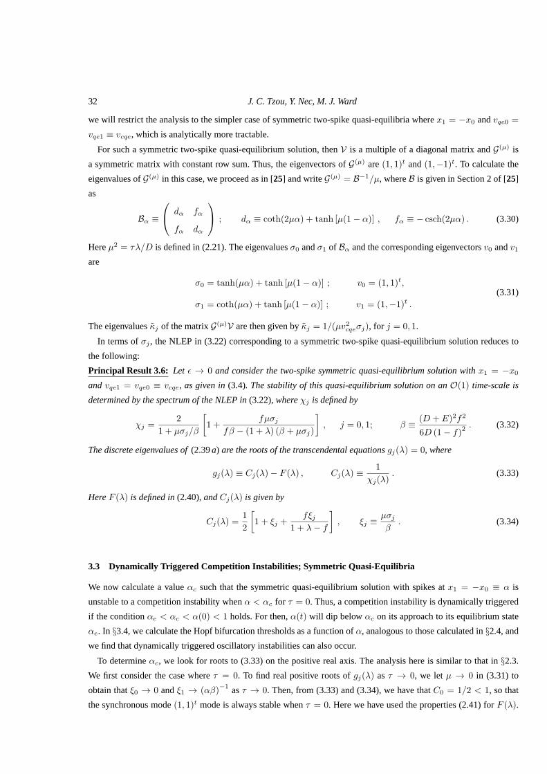
32 J. C. Tzou, Y. Nec, M. J. Ward
we will restrict the analysis to the simpler case of symmetric two-spike quasi-equilibria wherex1 = −x0 andvqe0 =
vqe1 ≡ vcqe, which is analytically more tractable.
For such a symmetric two-spike quasi-equilibrium solution, thenV is a multiple of a diagonal matrix andG(µ) is
a symmetric matrix with constant row sum. Thus, the eigenvectors ofG(µ) are(1, 1)t and(1,−1)t. To calculate the
eigenvalues ofG(µ) in this case, we proceed as in [25] and writeG(µ) = B−1/µ, whereB is given in Section 2 of [25]
as
Bα ≡
dα fα
fα dα
; dα ≡ coth(2µα) + tanh [µ(1− α)] , fα ≡ − csch(2µα) . (3.30)
Hereµ2 = τλ/D is defined in (2.21). The eigenvaluesσ0 andσ1 of Bα and the corresponding eigenvectorsv0 andv1
are
σ0 = tanh(µα) + tanh [µ(1− α)] ; v0 = (1, 1)t,
σ1 = coth(µα) + tanh [µ(1− α)] ; v1 = (1,−1)t .
(3.31)
The eigenvaluesκj of the matrixG(µ)V are then given byκj = 1/(µv2cqeσj), for j = 0, 1.
In terms ofσj , the NLEP in (3.22) corresponding to a symmetric two-spike quasi-equilibrium solution reduces to
the following:
Principal Result 3.6: Let ǫ → 0 and consider the two-spike symmetric quasi-equilibrium solution with x1 = −x0andvqe1 = vqe0 ≡ vcqe, as given in(3.4). The stability of this quasi-equilibrium solution on anO(1) time-scale is
determined by the spectrum of the NLEP in(3.22), whereχj is defined by
χj =2
1 + µσj/β
[
1 +fµσj
fβ − (1 + λ) (β + µσj)
]
, j = 0, 1; β ≡ (D + E)2f2
6D (1− f)2 . (3.32)
The discrete eigenvalues of(2.39a) are the roots of the transcendental equationsgj(λ) = 0, where
gj(λ) ≡ Cj(λ)− F (λ) , Cj(λ) ≡1
χj(λ). (3.33)
HereF (λ) is defined in(2.40), andCj(λ) is given by
Cj(λ) =1
2
[
1 + ξj +fξj
1 + λ− f
]
, ξj ≡µσjβ
. (3.34)
3.3 Dynamically Triggered Competition Instabilities; Symmetric Quasi-Equilibria
We now calculate a valueαc such that the symmetric quasi-equilibrium solution with spikes atx1 = −x0 ≡ α is
unstable to a competition instability whenα < αc for τ = 0. Thus, a competition instability is dynamically triggered
if the conditionαe < αc < α(0) < 1 holds. For then,α(t) will dip below αc on its approach to its equilibrium state
αe. In §3.4, we calculate the Hopf bifurcation thresholds as a function ofα, analogous to those calculated in§2.4, and
we find that dynamically triggered oscillatory instabilities can also occur.
To determineαc, we look for roots to (3.33) on the positive real axis. The analysis here is similar to that in§2.3.
We first consider the case whereτ = 0. To find real positive roots ofgj(λ) asτ → 0, we letµ → 0 in (3.31) to
obtain thatξ0 → 0 andξ1 → (αβ)−1 asτ → 0. Then, from (3.33) and (3.34), we have thatC0 = 1/2 < 1, so that
the synchronous mode(1, 1)t mode is always stable whenτ = 0. Here we have used the properties (2.41) forF (λ).
The Stability of Localized Spikes for the 1-D Brusselator Reaction-Diffusion Model 33
Alternatively, whenτ = 0, we have from (3.34) that
C1(λ) =1
2
[
1 + ξ1 +fξ1
1 + λ− f
]
, ξ1 ≡ 1/(αβ) . (3.35)
SinceC1(λ) is a positive decreasing function ofλwhileF (λ) has the properties in (2.41), theng1 has a unique positive
real root ifC1(0) > 1 and no roots ifC1(0) < 1. A winding number argument similar to that used in§2.3 can be used
to show that no other roots exist in the right-half plane. This leads to the following stability criteria:
Principal Result 3.7: For τ = 0, consider the quasi-equilibrium solution(3.4) to (1.5) with spikes centered atx =
±α for 0 < α < 1, and where the spikes have a common amplitude. The solution is stable on anO(1) time-scale if
and only if
α > αc; αc ≡6D(1− f)
(D + E)2f2. (3.36)
If the inequality in(3.36) is reversed, the quasi-equilibrium profile is unstable to one real positive eigenvalue cor-
responding to the(1,−1)t mode, which conserves the sum of the amplitudes of the spikes. Note that ifD ≪ 1 but
D ≫ O(ǫ2), we have thatαc ∼ 6D(1− f)/(E2f2) ≪ 1 so that the region of stability spans almost the entire range
0 < α < 1. Also, from(3.36), we see thatαc ∼ O(D−1) asD → ∞. We remark that the conditionα > αc is
equivalent to the conditionc > 2/√b in the analysis of the quasi-equilibria in (3.8).
As discussed earlier, a symmetric two-spike quasi-equilibrium solution can undergo a dynamic competition insta-
bility wheneverαe < αc < 1. By using the expression forαe in (3.16), we have the following result:
Principal Result 3.8: The quasi-equilibrium solution in(3.4) with a rightmost initial spike locationα(0) satisfying
α(0) > αc will undergo a dynamic competition instability at some timet > 0 whenαe < αc < 1. These inequalities
hold when
1
12
E
D
[
1 +D
E
]3
<1− f
Ef2<
1
6
E
D
[
1 +D
E
]2
. (3.37)
The region described by (3.37) is plotted in Figure 16. Abovethe dotted curve a competition instability occurs
starting att = 0 for anyα(0), while below the solid curve the two-spike quasi-equilibrium solution is stable to the
large eigenvalues and there is no competition instability for anyα(0) with α(0) > αe.
By comparing the lower bound of (3.37) with (3.17), we conclude that forτ = 0 the two-spike equilibrium solution
is stable if and only if it is stable to the small eigenvalues in the limit τ → 0. The result is written as:
Principal Result 3.9: The symmetric two-spike equilibrium solution in(3.4)withα = αe is stable with respect to the
large eigenvalues but unstable with respect to the small eigenvalues when
1
24
E
D
[
1 +D
E
]3
<1− f
Ef2<
1
12
E
D
[
1 +D
E
]3
. (3.38)
It is stable with respect to the small eigenvalues when(3.17)holds.
For the caseτ > 0, it is difficult, owing to the non-monotonicity of the curvesCj(λ), to obtain explicit results that
count the number of positive real eigenvalues in the right half-plane. However, the following (less precise) results are
readily proved.
Principal Result 3.10: Suppose thatτ ≥ 0 and that0 < α < αc. Then, the NLEP in Principal Result 3.3 admits
at least one real positive eigenvalue. Hence, the quasi-equilibrium pattern in unstable. Alternatively, suppose that
αc < α < 1. Then, forτ > 0 sufficiently large, the NLEP in Principal Result 3.3 admits four real positive eigenvalues.
To prove the first statement, we note thatC1(0) > 1 whenα < αc. Therefore, the curvesC1(λ) andF (λ) must
have at least one intersection inλ > 0 whenτ ≥ 0. To prove the second statement we notice thatCj(0) < 1 when

34 J. C. Tzou, Y. Nec, M. J. Ward
0 0.2 0.4 0.6 0.8 10
1
2
3
4
5
6
D/E
(1−
f)/
(Ef
2)
Figure 16. The region between the two curves is the parameterspace in which a dynamic competition instability is
possible for a two-spike pattern with initial stateα(0) with αe < α(0) < 1. The horizontal axis is on the range
0 < D/E < 1 for which a two-spike equilibrium solution exists.
α > αc for j = 0, 1 and thatCj(λ) = O(√
τλ)
for λ > 0 whenτ ≫ 1. It follows from the concavity ofCj(λ) in the
largeτ limit and the convexity ofF (λ) (see properties (2.41)) that for bothj = 0 andj = 1, there are two intersection
points ofCj(λ) = F (λ) on0 < λ < 5/4.
3.4 Dynamically Triggered Oscillatory Instabilities; Symmetric Quasi-Equilibria
For the parameter rangeαc < α < 1, we calculate the thresholdτ0 for which the NLEP has a complex conjugate pair
of eigenvalues on the imaginary axis. More specifically, we calculate the valuesτ = τ0j(α) such thatgj = 0 has a
pair of complex conjugate solutionsλ = ±iλ0Ij(α) on the imaginary axis. The quantity
τ0(α) = min(τ00, τ01) , (3.39)
is then defined to be the Hopf instability threshold. As in§2.4, either thej = 0 mode, which corresponds to syn-
chronous oscillations, or thej = 1 mode, which corresponds to asynchronous oscillations, canbe the dominant
instability, depending on the value ofα. In contrast, for the GM and GS models studied in [25] the synchronous mode
was always the dominant instability. Using the numerical procedure used to produce the Hopf bifurcation curves of
§2.4, we solvegj(iλI) = 0 to obtain curvesτ0j(α) andλ0Ij(α).
Treatingα as the independent variable, we fixD andE and generate Hopf curves for values off in the interval
fc < f ≤ 0.9, whereαc = 1 whenf = fc. In Figure 16, this corresponds to a vertical traversal fromthe dotted
curve down toward theD/E-axis. Results are presented on a semi-log plot for three ratios ofD/E. In Figures 17(a) -
17(c), we takeE = 1 andD = 0.2, 0.4 and0.6. Similar plots were made (not shown) for the same ratios ofD/E but
with D = 1 andE = 5, 2.5, 1.67, yielding qualitatively similar plots. For values ofα where the curves are solid, the
synchronous mode is the dominant instability (τ0 ≡ τ00), whereas for the portions of the curves where they are dashed,
the asynchronous mode is dominant (τ0 ≡ τ01). The curves are ordered such that for a givenα, τ0(α) increases with
increasingf . We end the plot forα < αc, that is, values ofα for which theτ01 curve does not exist; the corresponding

The Stability of Localized Spikes for the 1-D Brusselator Reaction-Diffusion Model 35
complex conjugate imaginary eigenvalues approach the origin asα → α+c the same way thatλ0I1 → 0 asD → D−
c2
as discussed in§2.4. The equilibrium locationαe is denoted by a dot; in the absence of a dot, the conditionαe < αc
is satisfied and a dynamic competition instability is possible. In Figure 17(a),τ00 and τ01 are almost equal forα
sufficiently near unity, and the breaks in the curves appear to be due to differences in decimal places beyond the
precision of the solver.
0 0.2 0.4 0.6 0.8 110
−1
100
101
102
103
α
τ 0
(a) D = 0.2, E = 1
0 0.2 0.4 0.6 0.8 110
0
101
102
103
α
τ 0
(b) D = 0.4, E = 1
0 0.2 0.4 0.6 0.8 110
0
101
102
103
α
τ 0
(c) D = 0.6, E = 1
Figure 17. Plot ofτ0 versusα for variousf with E = 1 andD = 0.2 (left), D = 0.4 (center) andD = 0.6 (right).
The extent of the curves inα increases inf , as does the value ofτ0 for any givenα. Forα where the curves are solid
(dashed), the dominant instability is the synchronous (asynchronous) mode. The dot denotes the equilibrium location
αe; for curves without a dot, a dynamic competition instability is possible. The values off are as follows: left figure:
f = 0.6181, 0.6494, 0.6808, 0.7121, 0.7434, 0.7747, 0.8060, 0.8374, 0.8687, 0.9000; center figure:f = 0.6772,
0.7019, 0.7267, 0.7514, 0.7762, 0.8010, 0.8257, 0.8505, 0.8752, 0.9000; right figure:f = 0.6980, 0.7204, 0.7429,
0.7653, 0.7878, 0.8102, 0.8327, 0.8551, 0.8776, 0.9000.
For a givenα, the quasi-equilibrium is stable (unstable) whenτ is below (above) the curve. Thus, because the spike
motion from (3.15) is directed monotonically towards the equilibrium location, dynamic oscillatory instabilities are
only possible when either the slope ofτ0 is negative whenα < αe or positive whenα > αe. From Figures 17(a)
- 17(c), we see that forf nearfc, the only possibility for a dynamic oscillatory instability is when the initial spike
locations satisfyα(0) > αe andτ satisfiesτ0(αe) < τ < τ0(α(0)) (or τ0(αc) < τ < τ0(α(0)) if αe < αc), leading
to the triggering of synchronous spike oscillations at somet > 0 asα → α+e . For largerf , a similar scenario is
possible for asynchronous oscillations. For still largerf , synchronous oscillations may be triggered when the initial
spike location satisfiesα(0) < αe. This may occur after passage through a region of instability to asynchronous
oscillations. In the next section, we illustrate these scenarios by numerically solving the full PDE system (1.5).
3.5 Numerical Validation: Symmetric Quasi-Equilibria
We now illustrate five different scenarios involving spike dynamics with parameters used to generate curves in Figure
17(a). For clarity, we reproduce the curves in Figure 18 on which we qualitatively annotate the dynamics ofα(t)
for each run. Below, we present the results of each run by plotting the spike amplitudesum and spike locationsxj
versus time, produced by solving (1.5) with4000 grid points usingMATLAB’s pdepe() solver. In all runs, we took
ǫ = 0.005, D = 0.2 andE = 1, with f andτ being varied between the runs. The initial conditions are treated in

36 J. C. Tzou, Y. Nec, M. J. Ward
the same way as described in§2.5, where the quasi-equilibrium solution in (3.4) is takenas the initial conditions, and
a small value ofτ is used to solve forward in time until a true quasi-equilibrium solution is reached. While the time
required for the initiation process is small compared toǫ−2, the spikes still drift during this time. As such, appropriate
compensations were made in the initial conditions so that the spike locations were in their desired locations at the end
of the initiation. All values for the initial spike locationsα(0) quoted below refer to their locations at the end of the
initiation.
0 0.2 0.4 0.6 0.8 1
100
101
α
τ 0
Run 1Run 2
Run 3
Run 5
Run 4
Figure 18. Hopf stability curves for (bottom to top)f = 0.6494, 0.7121, and0.806. The arrows indicate the evolution
of α(t), while the height of the arrows is only indicative of the value ofτ used in the runs. Runs 1 and 2 are associated
with the lowest curve, Run 3 with the middle curve, and Runs 4 and 5 with the top curve. Solid curves indicate that
τ0 ≡ τ00 (synchronous mode) while dashed curves indicate thatτ0 ≡ τ01 (asynchronous mode). The curves are cut off
on the left atα = αc. The equilibrium pointαe = 0.6 is indicated by a dot when the conditionαe > αc is satisfied.
In Run 1, we takeα(0) = 0.85, f = 0.6494, andτ = 1.05 < τ0(α(0)) so that the quasi-equilibrium is initially
stable att = 0. However, as indicated in Figure 18, our theory predicts that a dynamic synchronous oscillatory
instability is triggered at somet > 0 whenα decreases below the synchronous stability threshold indicated by the
solid curve in this figure. That is, for some timet > 0, the conditionτ > τ0(α(t)) is satisfied, at which time the
solution becomes unstable to synchronous oscillations. InFigure 19(a) we show the amplitudes of the two spikes,
which are indistinguishable, after the onset of the synchronous Hopf instability. The spikes annihilate beforeα reaches
αc, implying that the annihilation was not due to a competitioninstability. In Figure 19(b), we show a favorable
comparison between the slow time evolution of the location of the spikes and the dynamics in (3.15) before the time
of annihilation.
With the initial conditions and the other parameters unchanged, for Run 2 we decreaseτ to τ = 0.8 so that the Hopf
stability threshold is not crossed at any point in the dynamics. However, becauseαe < αc, a competition instability
occurs asα(t) decreases belowαc. This scenario is illustrated in Figure 18. In Figure 20(a),we show the annihilation
of one of the spikes after the thresholdα(t) < αc is crossed. In Figure 20(b), we show a favorable comparison between
the numerical spike dynamics and that predicted by (3.15) upto the time of the annihilation of the right spike. After
the annihilation, the remaining spike evolves according tothe one-spike dynamical result of [27].
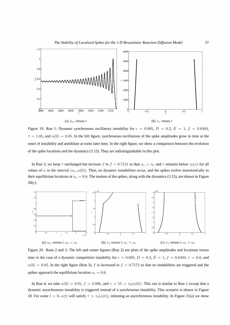
The Stability of Localized Spikes for the 1-D Brusselator Reaction-Diffusion Model 37
4800 4850 4900 4950 5000 5050 5100 51500
0.2
0.4
0.6
0.8
1
1.2
t
um
(a) um versust
−1 −0.5 0 0.5 10
1000
2000
3000
4000
5000
6000
x
t(b) xj versust
Figure 19. Run 1: Dynamic synchronous oscillatory instability for ǫ = 0.005, D = 0.2, E = 1, f = 0.6494,
τ = 1.05, andα(0) = 0.85. In the left figure, synchronous oscillations of the spike amplitudes grow in time at the
onset of instability and annihilate at some later time. In the right figure, we show a comparison between the evolution
of the spike locations and the dynamics (3.15). They are indistinguishable in this plot.
In Run 3, we keepτ unchanged but increasef to f = 0.7121 so thatαc < αe andτ remains belowτ0(α) for all
values ofα in the interval(αe, α(0)). Thus, no dynamic instabilities occur, and the spikes evolve monotonically to
their equilibrium locations atαe = 0.6. The motion of the spikes, along with the dynamics (3.15), are shown in Figure
20(c).
0 0.5 1 1.5 2 2.5
x 104
0
0.2
0.4
0.6
0.8
1
1.2
1.4
t
um
(a) um versust, αe < αc
−1 −0.5 0 0.5 10
0.5
1
1.5
2
2.5x 10
4
x
t
(b) xj versust, αe < αc
−1 −0.5 0 0.5 10
0.5
1
1.5
2
2.5
3
3.5
4x 10
4
x
t
(c) xj versust, αe > αc
Figure 20. Runs 2 and 3: The left and center figures (Run 2) are plots of the spike amplitudes and locations versus
time in the case of a dynamic competition instability forǫ = 0.005, D = 0.2, E = 1, f = 0.6494, τ = 0.8, and
α(0) = 0.85. In the right figure (Run 3),f is increased tof = 0.7172 so that no instabilities are triggered and the
spikes approach the equilibrium locationαe = 0.6.
In Run 4, we takeα(0) = 0.91, f = 0.806, andτ = 15 < τ0(α(0)). This run is similar to Run 1 except that a
dynamic asynchronous instability is triggered instead of asynchronous instability. This scenario is shown in Figure
18. For somet > 0, α(t) will satisfy τ > τ0(α(t)), initiating an asynchronous instability. In Figure 21(a) we show

38 J. C. Tzou, Y. Nec, M. J. Ward
asynchronous spike amplitude oscillations resulting fromthe triggering of an asynchronous Hopf instability. As in Run
1, the spikes annihilate at some time after onset but beforeα has reachedαc, implying that the annihilation was not
due to a competition instability. In Figure 21(b), we show a favorable comparison between the slow spike dynamics
before the annihilation event and that predicted by (3.15).For this run, we perturbed the initial condition as in (2.63),
whered0 = 1 andd1 = −1 in accordance with the eigenvector associated with the asynchronous mode. While the
perturbation initially decayed and appeared to be unnoticeable by the time the spikes approached the asynchronous
instability threshold, enough of the initial perturbationremained to trigger the asynchronous instability. Withoutthe
initial perturbation, a synchronous instability developed due to the nearby synchronous instability threshold (not shown
in Figure 18).
1100 1150 1200 1250 1300 1350 14000
0.5
1
1.5
t
um
(a) um versust
−1 −0.5 0 0.5 10
500
1000
1500
x
t
(b) xj versust
Figure 21. Run 4: Dynamic asynchronous oscillatory instability for ǫ = 0.005,D = 0.2, E = 1, f = 0.806, τ = 15,
andα(0) = 0.91. In the left figure, asynchronous oscillations of the left (solid) and right (dashed) spike amplitudes
grow in time at the onset of instability and annihilate at some later time. In the right figure, we show a comparison
between the evolution of the spike locations and the dynamics (3.15) up to the time of annihilation.
In Run 5, we keep the parameters as in Run 4, except we setα(0) = 0.28 andτ = 6.6 so thatτ > τ0(α(0)) = τ01.
Thus, the solution starts above the asynchronous stabilitythreshold but gains stability asα(t) increases towardsαe.
However, before reachingαe, a loss of stability to synchronous oscillations occurs before stability is regained after
α(t) drifts across the zone of synchronous instability. The evolution through the zones of stability and instability is
depicted in Figure 18. In Figures 22(a) and 22(b), we show thespike amplitudes and locations versus time for the en-
tire duration of the dynamics. Note that the spikes evolve according to (3.15) even whenα(t) is in an unstable region.
Figure 22(a) shows the triggering of two distinct types of instabilities, each of which are eventually extinguished as
time increases. The first of these instabilities, as previously mentioned, is to the asynchronous mode and is magnified
in Figure 22(c). The initial conditions were perturbed in the same way as in Run 4. After an initial growth in the
amplitude of asynchronous oscillations, the spike amplitudes approach their quasi-equilibrium value as they move into
the zone of stability. At a later time, shown in Figure 22(d),the spikes move into a zone of synchronous instability
where the amplitude of synchronous oscillations grow. These oscillations decay as the spikes move out of the unstable
region and towards their equilibrium locations. Note that the frequency of synchronous oscillations is approximately

The Stability of Localized Spikes for the 1-D Brusselator Reaction-Diffusion Model 39
four times that of the asynchronous oscillations, which is consistent with our calculations (not shown). In other exper-
iments, it was observed that starting too far above the asynchronous stability curve led to an annihilation of one of the
spikes. Further, the movement of the spikes through a zone ofinstability without annihilating may be facilitated by
ǫ sufficiently large; for smallǫ where the times spent in unstable regions are significantly longer, annihilation events
may occur.
Finally, we note that all of these experiments involve onlyO(1) instabilites. For numerical computations involving
instabilities toO(ǫ2) eigenvalues, see [27].
0 5000 10000 150001.18
1.19
1.2
1.21
1.22
1.23
1.24
1.25
1.26
1.27
1.28
t
um
(a) um versust
−1 −0.5 0 0.5 10
5000
10000
15000
x
t
(b) xj versust
0 200 400 600 800 10001.18
1.19
1.2
1.21
1.22
1.23
1.24
1.25
1.26
1.27
1.28
t
um
(c) um versust, first instability: asynchronous
8000 8200 8400 8600 8800 90001.18
1.19
1.2
1.21
1.22
1.23
1.24
1.25
1.26
1.27
1.28
t
um
(d) um versust, second instability: synchronous
Figure 22. Run 5: Synchronous and asynchronous instabilities forǫ = 0.005, D = 0.2, E = 1, f = 0.806, τ = 6.6,
andα(0) = 0.28. The top left figure shows the spike amplitudes as the spikes move through zones of stability and
instability and eventually to their equilibrium locations(top right). The first instability is to the asynchronous mode
(bottom left) and the second instability is to the synchronous mode (bottom right). In the bottom left figure, the
solid (dashed) curve is the amplitude of the left (right) spike. In the bottom right figure, the spike amplitudes are
indistinguishable.
40 J. C. Tzou, Y. Nec, M. J. Ward
4 Discussion
We have analyzed the stability of localized spike patterns for two closely related singularly perturbed RD systems with
Brusselator kinetics. The derivation of the NLEP for the Brusselator is more intricate than in previous stability analyses
of spike patterns for the GM and GS models [32, 30, 12], owing to the non-trivial background state for the activator
and the existence of two nonlocal terms arising from theO(ǫ−1) coefficient in (1.3b) and (1.5b). A combination of
rigorous and numerical analysis was used to obtain stability thresholds from this NLEP, and the results have been
confirmed with full numerical simulations of the PDE systems. For (1.5), an NLEP stability theory is applied to a
quasi-steady two-spike evolution, and our results show theexistence of dynamically triggered instabilities depending
on the parameter regime.
For both Brusselator models (1.5) and (1.3), our NLEP stability results show that asτ increases above a threshold,
a Hopf bifurcation triggers either a synchronous or an asynchronous oscillation in the spike amplitudes. The nature of
the oscillation depends on the parameter values off andD, and for (1.5), also on the inter-spike distance. Our full
numerical simulations of the PDE systems confirm the two modes of oscillation. Furthermore, our numerical results
suggest that the synchronous instability, which leads to the annihilation of spikes, is subcritical, while the asynchronous
instability is supercritical. The existence of robust asynchronous spike amplitude oscillations observed in our analysis
of the Brusselator model has not been reported in NLEP stability studies of other RD (cf. [32, 12]).
A key open problem, suggested by our results, is to perform a weakly nonlinear theory on the Brusselator model, and
on related RD systems with spike solutions, to analyze whether spike amplitude oscillations are sub- or super-critical.
Another interesting open problem is to try to extend the pulse-splitting analysis of [5, 16, 13] to analyze a similar
pulse-splitting phenomena for the Brusselator model (1.3)that occurs in the regime whef approaches unity. Starting
from a one-pulse quasi-equilibrium state, in Fig. 23 we shownumerical results computed from (1.3) for the parameter
setǫ = 0.01, A = 0, D = 0.02, f = 0.95, andτ = 0.001. Such a pulse-splitting behaviour has not been reported
previously for the Brusselator model.
A final open problem is to analyze (1.3) in a two-dimensional spatial domain, where localized spot patterns undergo
either self-replication, competition, or oscillatory, instabilities depending on the parameter regime. The determina-
tion of phase diagrams in parameter space for these instabilities is critical for characterizing dynamic bifurcationsof
localized spot patterns.
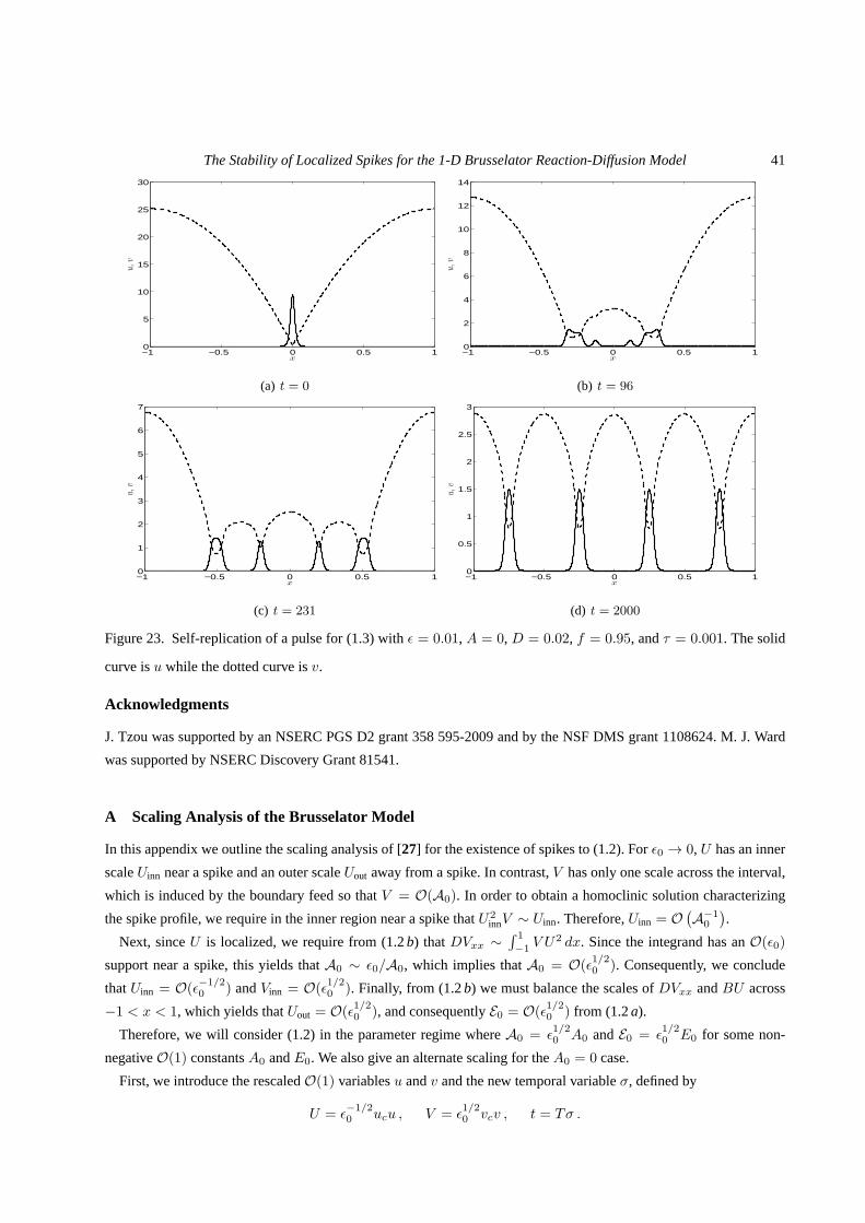
The Stability of Localized Spikes for the 1-D Brusselator Reaction-Diffusion Model 41
−1 −0.5 0 0.5 10
5
10
15
20
25
30
x
u,v
(a) t = 0
−1 −0.5 0 0.5 10
2
4
6
8
10
12
14
x
u,v
(b) t = 96
−1 −0.5 0 0.5 10
1
2
3
4
5
6
7
x
u,v
(c) t = 231
−1 −0.5 0 0.5 10
0.5
1
1.5
2
2.5
3
x
u,v
(d) t = 2000
Figure 23. Self-replication of a pulse for (1.3) withǫ = 0.01, A = 0,D = 0.02, f = 0.95, andτ = 0.001. The solid
curve isu while the dotted curve isv.
Acknowledgments
J. Tzou was supported by an NSERC PGS D2 grant 358 595-2009 andby the NSF DMS grant 1108624. M. J. Ward
was supported by NSERC Discovery Grant 81541.
A Scaling Analysis of the Brusselator Model
In this appendix we outline the scaling analysis of [27] for the existence of spikes to (1.2). Forǫ0 → 0, U has an inner
scaleUinn near a spike and an outer scaleUout away from a spike. In contrast,V has only one scale across the interval,
which is induced by the boundary feed so thatV = O(A0). In order to obtain a homoclinic solution characterizing
the spike profile, we require in the inner region near a spike thatU2innV ∼ Uinn. Therefore,Uinn = O
(
A−10
)
.
Next, sinceU is localized, we require from (1.2b) thatDVxx ∼∫ 1
−1V U2 dx. Since the integrand has anO(ǫ0)
support near a spike, this yields thatA0 ∼ ǫ0/A0, which implies thatA0 = O(ǫ1/20 ). Consequently, we conclude
thatUinn = O(ǫ−1/20 ) andVinn = O(ǫ
1/20 ). Finally, from (1.2b) we must balance the scales ofDVxx andBU across
−1 < x < 1, which yields thatUout = O(ǫ1/20 ), and consequentlyE0 = O(ǫ
1/20 ) from (1.2a).
Therefore, we will consider (1.2) in the parameter regime whereA0 = ǫ1/20 A0 andE0 = ǫ
1/20 E0 for some non-
negativeO(1) constantsA0 andE0. We also give an alternate scaling for theA0 = 0 case.
First, we introduce the rescaledO(1) variablesu andv and the new temporal variableσ, defined by
U = ǫ−1/20 ucu , V = ǫ
1/20 vcv , t = Tσ .

42 J. C. Tzou, Y. Nec, M. J. Ward
From (1.2), we then obtain the system
1
T (B0 + 1)uσ =
(
ǫ0√B0 + 1
)2
uxx +ǫ0E0
uc(B0 + 1)− u+
ucvcB0 + 1
vu2 , (A.1a)
√B0 + 1
u2cTvσ =
D0
√B0 + 1
u2cvxx +
√B0 + 1
ǫ0
(
B0
ucvcu− vu2
)
. (A.1b)
ChoosingT = 1/(B0 + 1) anducvc = B0 in (A.1), and defining the new parametersǫ,D, E, f , andτ as
ǫ ≡ ǫ0√B0 + 1
, D ≡ D0
√B0 + 1
u2c, E ≡ E0
uc√B0 + 1
, f ≡ B0
B0 + 1, τ ≡ (B0 + 1)3/2
u2c, (A.2)
we obtain the system
uσ = ǫ2uxx + ǫE − u+ fvu2 , −1 < x < 1 , ux(±1, σ) = 0 , (A.3a)
τvσ = Dvxx +1
ǫ
(
u− vu2)
, −1 < x < 1 , vx(±1, σ) = ±A0/vc , (A.3b)
valid forA0 ≥ 0. If A0 > 0, we choosevc = A0 so thatuc = B0/A0. Replacing the time variableσ with t in (A.3),
the Brusselator model with asymptotically small boundary feed of the inhibitor is written in the form (1.5) whereσ is
replaced byt, andǫ, f , E,D andτ are defined in terms of the original variables by (1.6).
Alternatively, if A0 = 0, we may chooseuc = E0/√B0 + 1 so thatvc = B0
√B0 + 1/E0, resulting in the
parameterE in (A.2) and (A.3) being unity. In this case, the Brusselatormodel with no flux boundary conditions is
(1.3) whereǫ, f ,D, andτ are as defined in (1.4).
References
[1] W. Chen, M. J. Ward,Oscillatory Instabilities and Dynamics of Multi-Spike Patterns for the One-Dimensional Gray-Scott
Model, Europ. J. Appl. Math20(2), (1999), pp. 187–214.
[2] A. Doelman, R. A. Gardner, T. J. Kaper,Large Stable Pulse Solutions in Reaction-Diffusion Equations, Indiana U. Math. J.,
50(1), (2001), pp. 443–507.
[3] A. Doelman, W. Eckhaus, T. J. Kaper,Slowly-Modulated Two-Pulse Solutions in the Gray-Scott Model I: Asymptotic Con-
struction and Stability, SIAM J. Appl. Math.,61(3), (2000), pp. 1080–1102.
[4] A. Doelman, W. Eckhaus, T. J. Kaper,Slowly Modulated Two-Pulse Solutions in the Gray–Scott Model II: Geometric Theory,
Bifurcations, and Splitting Dynamics, SIAM J. Appl. Math.,66(6), (2001), pp. 2036–2062.
[5] A. Doelman, R. A. Gardner, T. J. Kaper,Stability Analysis of Singular Patterns in the 1D Gray-Scott Model: A Matched
Asymptotic Approach, Physica D,122, (1998), pp. 1–36.
[6] A. Doelman, T. Kaper,Semistrong Pulse Interactions in a Class of Coupled Reaction-Diffusion Equations, SIAM J. Appl.
Dyn. Sys.,2(1), (2003), pp. 53–96.
[7] A. Doelman, T. J. Kaper, K. Promislow,Nonlinear Asymptotic Stability of the Semistrong Pulse Dynamics in a Regularized
Gierer-Meinhardt Model, SIAM J. Math. Anal.,38(6), (2007), pp. 1760–1787.
[8] D. Iron, M. J. Ward, J. Wei,The Stability of Spike Solutions to the One-Dimensional Gierer-Meinhardt Model, Physica D,
150(1-2), (2001), pp. 25–62.
[9] D. Iron, M. J. Ward,The Dynamics of Multi-Spike Solutions for the One-Dimensional Gierer-Meinhardt Model, SIAM J.
Appl. Math.,62(6), (2002), pp. 1924–1951.

The Stability of Localized Spikes for the 1-D Brusselator Reaction-Diffusion Model 43
[10] D. Iron, J. Wei, M. Winter,Stability Analysis of Turing Patterns Generated by the Schnakenberg model, J. Math. Biol.,49(4),
(2004), pp. 358–390.
[11] B. S. Kerner, V. V. Osipov,Autosolitions: A New Approach to Problem of Self-Organization and Turbulence, Kluwer Academic
Publishers, Dordrecht, (1994).
[12] T. Kolokolnikov, M. J. Ward, J. Wei,The Existence and Stability of Spike Equilibria in the One-Dimensional Gray-Scott
Model: The Low Feed Rate Regime, Studies in Appl. Math.,115(1), (2005), pp. 21–71.
[13] T. Kolokolnikov, M. J. Ward, J. Wei,The Existence and Stability of Spike Equilibria in the One-Dimensional Gray-Scott
Model: The Pulse-Splitting Regime, Physica D.,202(3-4), (2005), pp. 258–293.
[14] T. Kolokolnikov, M. J. Ward, J. Wei,The Stability of Steady-State Hot-Spot Patterns for a Reaction-Diffusion Model of Urban
Crime, DCDS-B, submitted, (2011), (34 pages).
[15] C. S. Lin, W. M. Ni, I. Takagi,Large Amplitude Stationary Solutions to a Chemotaxis System, J. Diff. Eq.,72, (1988), pp. 1–27.
[16] C. B. Muratov, V. V. Osipov,Static Spike Autosolitons in the Gray-Scott Model, J. Phys. A: Math. Gen.,33, (2000), pp. 8893–
8916.
[17] C. B. Muratov, V. V. Osipov,Stability of the Static Spike Autosolitons in the Gray–Scott Model, SIAM J. Appl. Math.,62(5),
(2002), pp. 1463–1487.
[18] G. Nicolis, I. Prigogine,Self-Organization in Nonequilibrium Systems, Wiley, New York, 1977.
[19] Y. Nishiura, Far-From Equilibrium Dynamics, Translations of Mathematical Monographs, Vol. 209, AMS Publications,
(2002), Providence, Rhode Island.
[20] B. Pena, C. Perez-Garcia,Stability of Turing Patterns in the Brusselator Model, Phys. Rev. E.,64, (2001), 056213
[21] R. Peng, M. Wang,Pattern Formation in the Brusselator System, J. Math. Anal. Appl.,309(1), (2005), pp. 151–166.
[22] R. Peng, M. Yang,On Steady-State Solutions of the Brusselator-Type System, Nonlinear Analysis: Theory, Methods, and
Appl., 71(3-4), (2009), pp. 1389–1394.
[23] C. P. Schenk, M. Or-Guil, M. Bode and H. Purwins,Interacting Pulses in Three-Component Reaction-Diffusion Systems on
Two-Dimensional Domains, Phys. Rev. Lett.,78(19), (1997), pp. 3781–3784.
[24] M. B. Short, A. L. Bertozzi, P. J. Brantingham,Nonlinear Patterns in Urban Crime - Hotpsots, Bifurcations, and Suppression,
SIAM J. Appl. Dyn. Sys.,9(2), (2010), pp. 462–483.
[25] W. Sun, M. J. Ward, R. Russell,The Slow Dynamics of Two-Spike Solutions for the Gray-Scott and Gierer-Meinhardt Systems:
Competition and Oscillatory Instabilities, SIAM J. Appl. Dyn. Sys.,4(4), (2005), pp. 904–953.
[26] J. C. Tzou, A. Bayliss, B. J. Matkowsky, V. A. Volpert,Interaction of Turing and Hopf Modes in the Superdiffusive Brusselator
Model Near a Codimension Two Bifurcation Point, Math. Model. Nat. Phenom.,6(1), (2011), pp. 87–118.
[27] J. C. Tzou, A. Bayliss, B. J. Matkowsky, V. A. Volpert,Stationary and Slowly Moving Localized Pulses in a Singularly
Perturbed Brusselator Model, European J. Appl. Math.,22(5), (2011), pp. 423–453.
[28] V. K. Vanag,Waves and Patterns in Reaction Diffusion Systems. Belousov-ZhabotinskyReaction in Water-in Oil Microemul-
sions, Phys.-Usp.47, (2004), pp. 923–941.
[29] V. K. Vanag, I. R. Epstein,Localized Patterns in Reaction-Diffusion Systems, Chaos,17(3), (2007), 037110.
[30] H. Van der Ploeg, A. Doelman,Stability of Spatially Periodic Pulse Patterns in a Class of Singularly Perturbed Reaction-
Diffusion Equations, Indiana Univ. Math. J.,54(5), (2005), pp. 1219-1301.
[31] M. J. Ward, J. Wei,The Existence and Stability of Asymmetric Spike Patterns for the Schnakenberg Model, Studies in Appl.
Math.,109(3), (2002), pp. 229–264.

44 J. C. Tzou, Y. Nec, M. J. Ward
[32] M. J. Ward, J. Wei,Hopf Bifurcations and Oscillatory Instabilities of Spike Solutions for the One-Dimensional Gierer-
Meinhardt Model, J. Nonlinear Sci.13(2), (2003), pp. 209–264.
[33] M. J. Ward, J. Wei,Hopf Bifurcation of Spike Solutions for the Shadow Gierer-Meinhardt Model, Europ. J. Appl. Math.,14(6),
(2003), pp. 677-711.
[34] J. Wei,On Single Interior Spike Solutions for the Gierer-Meinhardt System: Uniqueness and Spectrum Estimates, Europ. J.
Appl. Math.,10(4), (1999), pp. 353–378.
[35] J. Wei,Existence and stability of spikes for the Gierer-Meinhardt system, book chapter inHandbook of Differential Equations,
Stationary Partial Differential Equations, Vol. 5 (M. Chipot ed.), Elsevier, (2008), pp. 489–581.
[36] R. Wittenberg, P. Holmes,The Limited Effectiveness of Normal Forms: A Critical Review and Extension of Local Bifurcation
Studies of the Brusselator PDE, Physica D,100, (1997), pp. 1–40.