the statistics of causal inference: a view from political...

The Statistics of Causal Inference: A View fromPolitical Methodology

Luke Keele

Department of Political Science, 211 Pond Lab, Penn State University, University Park, PA 19130

e-mail: [email protected] (corresponding author)

Edited by R. Michael Alvarez

Many areas of political science focus on causal questions. Evidence from statistical analyses is often used

to make the case for causal relationships. While statistical analyses can help establish causal relationships,

it can also provide strong evidence of causality where none exists. In this essay, I provide an overview of the

statistics of causal inference. Instead of focusing on specific statistical methods, such as matching, I focus

more on the assumptions needed to give statistical estimates a causal interpretation. Such assumptions are

often referred to as identification assumptions, and these assumptions are critical to any statistical analysis

about causal effects. I outline a wide range of identification assumptions and highlight the design-based

approach to causal inference. I conclude with an overview of statistical methods that are frequently used for

causal inference.

1 Introduction

One central task of the scientific enterprise is establishing causal relationships. Take one examplefrom the comparative politics literature. One well-known finding is that democracies are less likelyto engage in the repression of human rights (Poe and Tate 1994). We can just treat this as adescriptive finding: democratic governance is correlated with lower levels of repression. This de-scriptive finding, however, begs a causal question: if a country becomes more democratic, will itthen engage in less repression? Rarely are we content with statistical associations. Instead, we oftenseek to establish causal relationships.

Causality is something we all understand, since we use it in our daily life. It refers to the rela-tional concept where one set of events causes another. Causal inference is the process by which wemake claims about causal relationships. While causality seems a simple concept in everyday life, theestablishment of causal relationships in many contexts is a difficult enterprise. Early models ofcausality focused on unique causes such as gravity. Gravity always causes things to fall to the earthand is the unique cause of that action. In biological and social applications, outcomes rarely haveunique causes, as causes tend to be contingent. In such contexts, the counterfactual model ofcausality is useful. Under the counterfactual model, rather than define causality purely in termsof observable events, causation is defined in terms of observable and unobservable events. Thus, Isay, if Iraq had been democratic, war would not have broken out. This is a counterfactual state-ment about the world that asserts that if a cause had occurred an effect would have followed. Thiscounterfactual approach is based on the idea that some of the information needed to make a causalinference is unobserved and thus some assumptions must be made before I can make a causalinference.1

Authors’ note: For comments I thank the editors and the four anonymous reviewers. I also thank Rocıo Titiunik, JasjeetSekhon, Paul Rosenbaum, and Dylan Small for many insightful conversations about these topics over the years. In theonline Supplementary Materials, I provide further information about software tools to implement many of themethodologies discussed in this essay. Supplementary materials for this article are available on the Political AnalysisWeb site.1See Hidalgo and Sekhon (2011) for an overview of different models of causality and the rise of the counterfactualmodel.

Advance Access publication April 22, 2015 Political Analysis (2015) 23:313–335doi:10.1093/pan/mpv007

� The Author 2015. Published by Oxford University Press on behalf of the Society for Political Methodology.All rights reserved. For Permissions, please email: [email protected]

313

at Pennsylvania State University on A

ugust 13, 2015http://pan.oxfordjournals.org/

Dow

nloaded from

http://pan.oxfordjournals.org/lookup/suppl/doi:10.1093/pan/mpv007/-/DC1

http://pan.oxfordjournals.org/lookup/suppl/doi:10.1093/pan/mpv007/-/DC1

http://pan.oxfordjournals.org/

In the social sciences, data and statistical analyses are often used to test causal claims. Over thelast 20 years, the potential outcomes framework, a manifestation of the counterfactual model ofcausality, has come to dominate statistical thinking about causality. What is behind the popularityof this approach? Why do some, myself included, view this framework as an improvement over thepast and not simply a “re-labeling” of existing statistical concepts? First, the counterfactualapproach has provided new insights into the assumptions needed for data to be informativeabout causality. Specifically, there has been a renewed interest in the assumptions needed forcausal inference and unpacking the exact meaning of those assumptions. Second, there has beena renewed emphasis on research design and the design-based approach. As I discuss below, thephrase “design-based approach” does not have universal definition, but there is widespread agree-ment that statistical analyses are more convincing when the research design has been carefullyconstructed to bolster assumptions before estimation.

In this essay, I provide a roadmap to the statistics of causal inference. I divide the statistics ofcausal inference into three parts: causal identification, the design-based approach, and statisticaltools. I begin with an introduction to the concept of causal identification and identificationanalyses. An identification analysis identifies the assumptions needed for statistical estimatesto be given a causal interpretation. Next, a researcher must select an identification strategy orresearch design. In this section, I also provide a brief overview of several common identificationstrategies.

Once an identification strategy has been selected, the analyst can often use elements of thedesign-based approach to improve the research design. The design-based approach is a set oftechniques that can make identification more credible without the use of parametric statisticalmodels and without using outcomes. Finally, I provide a brief overview of statistical tools likematching and inverse probability (IP) weighting, which are commonly used for the final part of acausal analysis: estimation of treatment effects. In this section, I also review how the mode ofstatistical inference changes when the focus is on causal effects. Through this structure, I clarifythe distinctions among identification, design, and statistical analysis.

2 Identification

I begin with a summary of identification, which is an extremely important concept in causal infer-ence. One way to describe whether a statistical estimate can be given a causal interpretation is todiscuss whether its target causal estimand, defined below, is identified or not. Identificationconcepts are invoked (often implicitly) in any analysis that purports to present a causal effect.Confusion often develops, however, since the concept of identification is more general.Identification problems arise in a number of different settings in statistics. I start with a generaldiscussion of identification, but then outline the specific identification problem that underlies causalinference.

2.1 Basics of Identification

Informally, we say a parameter in a model is identified if it is theoretically possible to learn the truevalue of that parameter with an infinite number of observations (Matzkin 2007, sec. 3.1).Conversely, for problems of identifiability, there are cases where even if we have an infinitenumber of observations, we don’t have enough information to learn about the true value of aparameter in the model. Manski (1995) separates the problem of inference into two components:identification and statistical. Under the identification part of inference, we seek to describe theconclusions that can be drawn with an infinite sample. If identification fails, nothing can be learnedeven if the sample is infinite. Studies of statistical inference, on the other hand, focus on what can belearned with finite samples.

There are many identification problems in statistics. For example, studies of ecological inferenceare based on an identification problem, where one attempts to identify the parameters of mixturesof probability distributions using only knowledge of the marginal distributions. This type of iden-tification problem occurs when we attempt to make inferences about units based on aggregates such

L. Keele314



Dow

nloaded from


as inferences about voters based on aggregating voting data. Inferences based on missing data forma different identification problem. Causal inference is yet another identification problem.Importantly, the causal inference identification problem can only be resolved through assumptions,which is not always the case for other identification problems. Consider the identification problemcreated by missing data. We can solve that identification problem using a set of assumptions aboutthe missing data. Alternatively, we might alter the data collection process such that no data aremissing, thus avoiding the use of assumptions. Under causal inference, there is no alternativemethod to resolve the identification problem other than through assumptions, since certain coun-terfactual quantities are unobservable.

To understand whether causal identification holds, we must perform an identification analysis. Inan identification analysis, we consider whether it is possible to compute a causal effect from datawith an infinite sample. In an identification analysis, the analyst provides both a formal statementof the set of assumptions needed to identify a particular causal effect and a proof that thoseassumptions lead to an identified causal effect. For example, one could state and prove the as-sumptions that must hold to compute a causal effect from a randomized experiment conducted withan infinite sample. More commonly one invokes an existing identification analysis and stipulatesidentification under that set of assumptions.

Often analysts perform a nonparametric identification analysis. In a nonparametric identificationanalysis, we formally prove which non-model-based (functional form) assumptions are needed foridentification.2 Nonparametric identification analyses are considered important since they allowone to state the weakest set of assumptions needed for identification. Nonparametric identificationassumptions are the assumptions that must hold to compute a causal effect with some hypotheticalset of data that is infinite in size and without reference to any specific statistical model. As I willoutline later, nonparametric identification often leads to a preference for nonparametric estimationmethods.

Next, I consider the source of the identification problem in causal inference. The potentialoutcomes framework (see, e.g., Rubin 1974), often referred to as the Rubin Causal Model(RCM) (Holland 1986), is one way to formalize the causal inference identification problem. TheRCM is the dominant model of causality in statistics at the moment. Like all models it is wrong, butit is also quite useful. In fact, the RCM is not the only model of causality that is embedded within astatistical framework. Dawid (2000) develops a decision theoretic approach to causality that rejectscounterfactuals. Pearl (1995, 2009a) advocates for a model of causality based on nonparametricstructural equations and path diagrams.

In the potential outcomes model, each unit has multiple potential outcomes but only one actualoutcome. Potential outcomes represent unit-level behavior in the presence or absence of an inter-vention or treatment, and the actual outcome depends on actual treatment received. I denote abinary treatment with Di 2 f0; 1g, though the treatment need not be binary. The potential outcomesare YiD. The actual outcome is a function of treatment assignment and potential outcomes suchthat Yi ¼ DiYi1 þ ð1�DiÞYi0. Under this framework, we can define various forms of the unit-levelcausal effect of Di, which are comparisons of unit-level potential outcomes. One possible compari-son is a difference in potential outcomes, Yi1 � Yi0, but in general the comparisons can take dif-ferent forms, such as a ratio: Yi1=Yi0.

We cannot estimate this unit-level causal effect since we do not observe the potential outcomes.The potential outcomes model formalizes the idea that the individual-level causal effect of Di isunobservable, which is sometimes called the fundamental problem of causal inference and encapsu-lates the identification problem we face as causal inferences are based on comparisons of counter-factual quantities that can’t be observed (Holland 1986). In general, we focus on the averagetreatment effect (ATE):

ATE ¼ E ½Yi1 � Yi0�: ð1Þ

2Linearity and additivity, for example, are model-based functional form assumptions.

The Statistics of Causal Inference 315



Dow

nloaded from


This is known as a causal estimand, since it based on a contrast of potential outcomes. It is separatefrom a statistical estimator or a specific point estimate that would be derived from observable data.In an identification analysis, we seek to identify specific estimands. The ATE is the average differ-ence in the pair of potential outcomes averaged over the entire population of interest. Often causalestimands are defined as averages over specific subpopulations. For example, we might averageover subpopulations defined by pretreatment covariates such as sex and estimate the ATE forfemales only. When the estimand is defined for a specific subpopulation, it is said to be morelocal. Frequently, the ATE is defined for the subpopulation exposed to the treatment or theATE on the treated (ATT):

ATT ¼ E ½Yi1 � Yi0jDi ¼ 1�: ð2Þ

Finally, we can define the relevant subpopulation in terms of potential outcomes. As I discuss later,the most well-known estimand to be defined in terms of a subpopulation based on potentialoutcomes comes from instrumental variables (IVs).3

I should note that I have followed common practice and written the estimands as averages.Causal identification rarely implies that only the middle (as represented by an average) of thetreated and control distributions will differ. Analysts should always consider that causal effectsmight only be apparent at particular quantiles. I revisit this topic later when I consider methods ofinference for causal effects.

For all these estimands, we face an identification problem, since there are terms in the estimandthat are unobservable. Even if we had samples of infinite size, we still could not estimate the averagecausal effect without observing both potential outcomes. Using potential outcomes, we can clearlyelucidate the unobservable quantities in the ATE estimand. I define � as the proportion of thesample assigned to the treatment condition. Using �, I can decompose the true ATE as a functionof potential outcomes as follows:

E ½Yi1 � Yi0�

¼ pfE ½Yi1jDi ¼ 1� � E ½Yi0jDi ¼ 1�g þ ð1� pÞfE ½Yi1jDi ¼ 0� � E ½Yi0jDi ¼ 0�g:ð3Þ

In equation (3), the ATE is a function of five quantities. Without additional assumptions we canestimate only three of those quantities directly from observed data. We can estimate � using E½Di�.We can also readily estimate E ½Yi1jDi ¼ 1� and E ½Yi0jDi ¼ 0� using E ½YijDi ¼ 1� and E ½YijDi ¼ 0�.However, we cannot estimate E ½Yi1jDi ¼ 0� and E½Yi0jDi ¼ 1� from the data without assumptions.One is the average outcome under treatment for those units in the control condition, and the otheris the average outcome under control for those in the treatment condition. That is, we face anidentification problem, since these two quantities are unobserved counterfactuals, and no add-itional amount of data will allow us to estimate these quantities. Therefore, we must find a setof assumptions that allow for identification.

In causal inference, identification generally rests on the assumption that treatment status isindependent of potential outcomes. Formally, this assumption is

Yi1;Yi0oDi: ð4Þ

Why does this assumption identify causal effects? The expectation of the observed outcome con-ditional on Di¼ 1 can be written as

E ½YijDi ¼ 1� ¼ E ½Yi0 þDiðYi1 � Yi0ÞjDi ¼ 1�

¼ E ½Yi1jDi ¼ 1�

¼ E ½Yi1�;

ð5Þ

3Here, I implicitly invoke the SUTVA, which permits the assumption that we are actually observing the potentialoutcomes associated with each treatment condition. I discuss SUTVA in more detail later in this section.

L. Keele316



Dow

nloaded from


where the last step follows from the assumption of independence. That is, taking the expectation of

the observed outcome provides the expectation of the potential outcome when independence holds.

Independence between treatment status and potential outcomes allows us to connect the observed

outcomes to the potential outcomes. By the same logic, E ½YijDi ¼ 0� ¼ E ½Yi0�. It follows from the

above statements that

ATE ¼ E ½Yi1 � Yi0�

¼ E ½Yi1� � E ½Yi0�

¼ E ½YijDi ¼ 1� � E ½YijDi ¼ 0�:

ð6Þ

That is, under the assumption of independence, the expectation of the unobserved potential

outcomes is equal to the conditional expectations of the observed outcomes conditional on treat-

ment assignment. The independence assumption allows us to connect unobservable potential

outcomes to observed quantities in the data, though one additional assumption is also needed. I

outline that additional assumption in the next section. When are we justified in assuming that

independence holds between the treatment and the potential outcomes? I take up that question

in the next section on identification strategies.While independence between treatment and potential outcomes is one assumption often used for

identification, typically additional assumptions are necessary for identification. Typically, we must

also assume that the stable unit treatment value assumption (SUTVA) holds (Rubin 1986). SUTVA

is made up of the two following components: (1) there are no hidden forms of treatment, which

implies that for unit i under Di¼ d, we assume that Yid ¼ Yi and (2) a subject’s potential outcome is

not affected by other subjects’ exposure to the treatment.The first component of SUTVA is often referred to as the consistency assumption in the epi-

demiological literature, and under this assumption we assume that for units exposed to a treatment

we observe the potential outcomes for that treatment. The consistency assumption is somewhat

controversial. Hernan and VanderWeele (2011) argue that the consistency assumption must be

evaluated by analysts since it links observed data to the counterfactual outcomes. They argue

that in the absence of consistency, one would not know which counterfactual contrast is being

estimated by the data, which makes it difficult to base decision-making on a causal analysis. For

example, if the treatment were “15min of exercise,” there are many different forms of exercise. They

contend that it will be difficult to justify any decision-making based on effect estimates since we may

not know which form of exercise actually made the treatment effective. In contrast, van der Laan,

Haight, and Tager (2005) say that consistency is an axiom which can be taken for granted, while

Pearl (2010) maintains that consistency immediately follows so long as the causal model is correct.

In some sense, there are elements of truth to both sides. If potential outcomes are independent of

the exercise treatment, we can rule out the presence of other causes. However, generating policy

recommendations about this treatment may be difficult given the fact that the treatment may

contain a large number of components.The second part of the SUTVA assumption tends to be a more serious problem in many social

science settings. The problem is that if we treat a unit and that unit can then spread some of that

treatment to a control unit or units, the comparison is no longer between treated and control, but

between a treated unit and partially treated unit. If one specifies a model of contagion for how the

treatment spreads, one can make some progress toward identification, but if we have no knowledge

of treatment spillovers, causal parameters will not be identified. Taking interference into account is

currently a very active area of research in both the social sciences and statistics (Sinclair,

McConnell, and Green, 2012; Tchetgen and VanderWeele 2012; Bowers, Fredrickson, and

Panagopoulos 2013). Treatments that vary over time can also lead to SUTVA violations, as well

as other complications. There has been considerable focus on treatments that vary over time in the

biostatistics literature, and I suspect time-varying treatments will eventually be a topic of interest in

political science (Robins 1997, 1999).Next, I briefly review the two most common threats to identification. The first is confounding

due to a common cause. Figure 1a contains a causal diagram of confounding. Confounding in




Dow

nloaded from


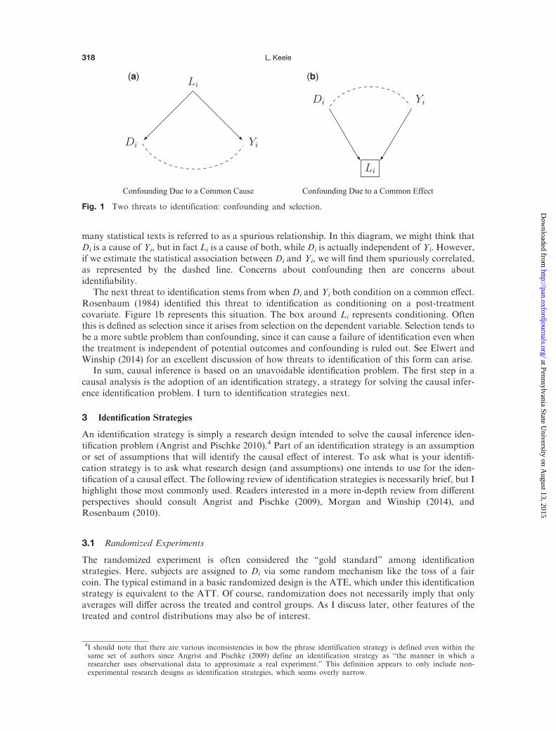
many statistical texts is referred to as a spurious relationship. In this diagram, we might think thatDi is a cause of Yi, but in fact Li is a cause of both, while Di is actually independent of Yi. However,if we estimate the statistical association between Di and Yi, we will find them spuriously correlated,as represented by the dashed line. Concerns about confounding then are concerns aboutidentifiability.

The next threat to identification stems from when Di and Yi both condition on a common effect.Rosenbaum (1984) identified this threat to identification as conditioning on a post-treatmentcovariate. Figure 1b represents this situation. The box around Li represents conditioning. Oftenthis is defined as selection since it arises from selection on the dependent variable. Selection tends tobe a more subtle problem than confounding, since it can cause a failure of identification even whenthe treatment is independent of potential outcomes and confounding is ruled out. See Elwert andWinship (2014) for an excellent discussion of how threats to identification of this form can arise.

In sum, causal inference is based on an unavoidable identification problem. The first step in acausal analysis is the adoption of an identification strategy, a strategy for solving the causal infer-ence identification problem. I turn to identification strategies next.

3 Identification Strategies

An identification strategy is simply a research design intended to solve the causal inference iden-tification problem (Angrist and Pischke 2010).4 Part of an identification strategy is an assumptionor set of assumptions that will identify the causal effect of interest. To ask what is your identifi-cation strategy is to ask what research design (and assumptions) one intends to use for the iden-tification of a causal effect. The following review of identification strategies is necessarily brief, but Ihighlight those most commonly used. Readers interested in a more in-depth review from differentperspectives should consult Angrist and Pischke (2009), Morgan and Winship (2014), andRosenbaum (2010).

3.1 Randomized Experiments

The randomized experiment is often considered the “gold standard” among identificationstrategies. Here, subjects are assigned to Di via some random mechanism like the toss of a faircoin. The typical estimand in a basic randomized design is the ATE, which under this identificationstrategy is equivalent to the ATT. Of course, randomization does not necessarily imply that onlyaverages will differ across the treated and control groups. As I discuss later, other features of thetreated and control distributions may also be of interest.

Confounding Due to a Common Cause Confounding Due to a Common Effect

(a) (b)

Fig. 1 Two threats to identification: confounding and selection.

4I should note that there are various inconsistencies in how the phrase identification strategy is defined even within thesame set of authors since Angrist and Pischke (2009) define an identification strategy as “the manner in which aresearcher uses observational data to approximate a real experiment.” This definition appears to only include non-experimental research designs as identification strategies, which seems overly narrow.

L. Keele318



Dow

nloaded from


See Rosenbaum (2010, chap. 2) and Gerber and Green (2012) for details on experiments. Here, Iwant to convey what is special about this identification strategy. The key strength of experiments isthat the researcher has the ability to impose independence between treatment status and potentialoutcomes on a set of units because he or she can impose a particular type of assignment process. AsI outlined above, if the treatment is independent of the potential outcomes, then the treatment effectparameter is identified. Short of incorrectly generating random treatment assignments, under thisidentification strategy the analyst knows that independence holds, which allows the researcher toassert that the treated and control groups will be identical in all respects, observable and unobserv-able, save receipt of the treatment with arbitrarily high probability as the sample size grows large.This implies that randomization allows us to rule out confounding due to a common cause.

Of course, randomization is not a cure-all. We must assume SUTVA holds. Moreover, experi-ment may not give valid causal estimates when attrition is present. Attrition is when subjectoutcomes are not available after randomization, and this missingness is correlated with treatmentstatus. Another complication in experiments is noncompliance. It is often the case that subjects donot comply with their assigned treatment status. A full discussion of noncompliance and attrition isbeyond the scope of this article. See Gerber and Green (2012) for a detailed discussion of bothtopics. Later I discuss noncompliance in more detail, since it forms a separate identificationstrategy.

Finally, a randomized experiment identifies the treatment effect within the population used in thestudy. This treatment effect may or may not extrapolate to other populations. To ensure validextrapolation, one either needs random sampling in addition to randomization of treatment oradditional assumptions. Given this fact, experiments are often said to be internally valid, but theymay lack external validity (Campbell and Stanley 1963). Whether this is a feature or a bug is amatter of substantial disagreement. Many of those who label themselves as interested in causalinference tend to value internal validity over external validity. If our concern is observing a causaleffect, we might place more value on a well-executed laboratory experiment than an observedassociation from a very large representative sample of data. As we will see, some identificationstrategies explicitly work based on comparisons of comparable but unrepresentativesubpopulations. I explain the logic behind the value placed on internal validity in the next section.

3.2 Natural Experiments

The next identification strategy is based on natural experiments. A natural experiment is a real-world situation that produces haphazard assignment to a treatment (Rosenbaum 2010, 67). Thehope is that a natural intervention will create as-if randomized treatment assignment and therebyproduce independence between treatment assignment and unit level potential outcomes. Of course,randomization in an experiment is a fact, while haphazard treatment assignment often requiresconsiderable judgment to justify it as as-if random. The circumstances of the natural experimentspeak to whether the claim of as-if random assignment is credible, but there is no way to knowwhether assignment is as good as randomized. An example is helpful.

Lyall (2009) seeks to understand whether indiscriminate violence increases insurgent attacks. Tothat end, he exploits shelling patterns by Russian troops in Chechnya that appear to be at worstindiscriminate and at best as-if random. He does find that the treatment, being shelled, appears tobe uncorrelated with pre-treatment covariates, as would be the case in a randomized experiment.The difficulty is that, unlike with randomization, we don’t know whether the patterns are trulyrandom since they are beyond the control of the analyst. As such, natural experiments often requirecareful justification for the as-if random nature of assignment. The basic template, however, ispresent in the study by Lyall (2009). He finds a real-world situation that appears to mimic arandomized experiment. Exploiting such circumstances is often a very credible identificationstrategy. Like randomized experiments, the focus is on internal validity. We have no way ofknowing whether the causal effect in Chechnya would hold in another circumstance, but whatwe hope to observe is a causal effect operating in relative isolation from the very real threats ofconfounding.




Dow

nloaded from


3.3 Instrumental Variables

Informally, an instrument is a random push to accept a treatment, but the push can only affect theoutcome if it induces units to take the treatment. Holland (1988) outlined the randomized encour-agement design as the prototype of an instrument. He described this design as an experiment wheresome participants are encouraged to exercise. While subjects are randomly encouraged to exercise,subjects then select their exposure to the exercise treatment in that they select whether to exercise ornot. Moreover, some of those assigned to the non-exercise arm will decide to exercise. Later allparticipants are measured on the outcome.

There are two effects of interest in designs of this type. In this design, the effect of being assignedto encouragement is identified since this has been randomly assigned. This estimand is often calledthe intention-to-treat (ITT) effect. This estimand tells us whether encouragement changes theoutcome. Under additional assumptions, the method of IV identifies the effect of the treatment,exercise, as opposed to the effect of being assigned to exercise encouragement (Angrist, Imbens, andRubin 1996). Specifically, IV identifies the average effect among those induced to take the treatmentby a randomized encouragement. The IV estimand is often referred to as either the complieraverage causal effect (CACE) or the local ATE (LATE). The IV estimand is local since it isdefined for a subpopulation: the compliers. However, this subpopulation is defined in terms ofpotential outcomes, since compliance status is unobservable for any particular unit (Angrist,Imbens, and Rubin 1996).

For IV to provide valid causal inferences, the five assumptions outlined by Angrist, Imbens, andRubin (1996) must hold. The assumptions needed for the IV estimand to be identified are (1)ignorable (as-if random) assignment of the encouragement; (2) the SUTVA; (3) no direct effectof the instrument (here, encouragement) on the outcome also known as the exclusion restriction;(4) monotonicity; and (5) the instrument must have a nonzero effect on the treatment. The first twoassumptions are identical to those needed to identify the ITT effect. The other three are additionalassumptions needed to identify the CACE.

Real-life circumstances can create circumstances that mimic the randomized encouragementdesign. More broadly, we can define an instrument as a haphazard nudge to accept a treatment.Here, IV becomes identification strategy based on a type of natural experiment. Hansford and Gomez(2010) are one example of using IV as a natural experiment identification strategy. They seek tounderstand whether lower turnout reduces the vote share for the Democratic Party. They exploit thefact that rainfall appears to decrease turnout on election day; and use it as an as-if random discour-agement for turnout. If rainfall is a valid instrument, this allows them to identify the local effect ofturnout on vote share among the counties discouraged to vote by rain on election day. While the IVidentification strategy can be credible, when used as a natural experiment it requires great care. SeeBound, Jaeger, and Baker (1995) for one example of a fairly spectacular failure of IV. See Sovey andGreen (2011) for a more detailed overview of the IV identification strategy.

One important insight that originated in the statistical literature on IVs was the role of implicitconstant effect assumptions. Angrist, Imbens, and Rubin (1996) clearly demonstrated that regres-sion-based IV estimates required an assumption that the effect of the treatment was constant acrossunits. They showed that under the nonparametric potential outcomes framework such assumptionscould be relaxed. This insight has led to closer examination of implicit constant effects assumptionsin many other identification strategies.

3.4 Regression Discontinuity Designs

The regression discontinuity (RD) design is another identification strategy that is typically classifiedas a type of natural experiment. In an RD design, assignment of the binary treatment, Di, is afunction of a known continuous covariate, Si, usually referred to as the forcing variable or the score.In the sharp RD design, treatment assignment is a deterministic function of the score, where allunits with score less than a known cutoff, c, are assigned to the control condition (D¼ 0) and allunits above the cutoff are assigned to the treatment condition (Di¼ 1). In the fuzzy RD design,assignment to the treatment is a random variable given the score, but the probability of receiving

L. Keele320



Dow

nloaded from


treatment conditional on the score, PðDi ¼ 1jSiÞ, must jump discontinuously at c. This implies thatit is possible for some units with scores below c to receive the treatment. The fuzzy RD designresults in an equivalence between RD and IV (Hahn, Todd, and van der Klaauw 2001). See Lee andLemieux (2010) for a much lengthier description of RD designs.

Hahn, Todd, and van der Klaauw (2001) demonstrate that for the sharp RD design to beidentified the potential outcomes must be a continuous function of the score in the neighborhoodaround the discontinuity. Under this continuity assumption, the potential outcomes can be arbi-trarily correlated with the score, so that, for example, people with higher scores might have higherpotential gains from treatment. The continuity assumption is a formal statement of the idea thatindividuals very close to the cutoff but on opposite sides of it are comparable or good counterfac-tuals for each other. Thus, continuity of the conditional regression function is enough to identifythe causal effect at the cutoff. The idea is that if nothing in the potential outcomes changes abruptlyat the cutoff other than the probability of receiving treatment, any jump in the conditional expect-ation of the outcome variable at the cutoff is attributed to the effects of the treatment. Often it isassumed that there is a neighborhood around the cutoff where treatment status is considered asgood as randomly assigned. Such an interpretation requires an additional identification assumption(Cattaneo, Frandsen, and Titiunik 2014). Here, the analyst must choose a neighborhood or windowaround the cutoff where treatment status is assumed to be as-if randomly assigned.

The RD design is another example of where the estimand changes as a function of the design.The RD design identifies a LATE for the subpopulation of individuals whose value of the score is ator near c, so the estimand is restricted to a subset of units on either side of the threshold that arethought to be good counterfactuals. In this design, it is only possible to identify the treatment effectamong a small subpopulation around the cutoff. Here, complications can arise since unmodelednonlinearity can be mistaken for a treatment effect. See Angrist and Pischke (2010) for an exampleof this.

Lee and Lemieux (2010) note that one strength of the RDD is that it is a design. Like random-ization, some decision-maker must implement a treatment assignment mechanism based on a con-tinuous score and a cutoff for a population of subjects. Lee and Lemieux (2010) emphasize thisaspect of an RDD which distinguishes it from many natural experiments that rely on an instrumentsuch as rainfall, which is certainly stochastic in some sense, but is not a controlled treatmentassignment mechanism. Moreover, RD designs have gained further credibility by recovering ex-perimental benchmarks (Cook, Shadish, and Wong 2008). However, see Caughey and Sekhon(2011) for one example where the assumptions of an RD design fail.

3.5 Selection on Observables

Under the “selection on observables” identification strategy, the analyst asserts that there is someset of covariates such that treatment assignment is random conditional on these covariates(Barnow, Cain, and Goldberger 1980). Under this assumption, there are no unobservable differ-ences between the treated and control groups. This assumption has a number of different names,which include “conditional ignorability” and “no omitted variables.” All of these are statements ofthe same idea: we seek to make the treatment independent of the potential outcomes conditional onobserved covariates. Under this identification strategy, we assume that the treatment is condition-ally independent of potential outcomes. Critically, the selection on observables assumption isnonrefutable, insofar as it cannot be verified with observed data (Manski 2007).

Given this set of “correct” covariates, we can use statistical adjustment methods such as regres-sion, matching, or weighting to make conditional independence hold. In regression terms, thisimplies that we tend to prefer longer specifications to shorter specifications. Of course, there aredangers in pursuing overly long specifications. While we need to include all covariates that predictthe outcome and treatment, we cannot condition on any covariates that are affected by treatment(Rosenbaum 1984) without further assumptions. Even in a randomized experiment, conditioningon covariates that are affected by the treatment will bias our estimate of the treatment effect. This issometimes known as over or bad control. See Angrist and Pischke (2009, 69) for an accessiblereview of the formal statement of the bias that arises from controlling for post-treatment covariates.




Dow

nloaded from


In an experiment, we can clearly delineate between the pre-treatment and post-treatment timeperiods. In observational data, that is often more difficult. In survey data, for example, it can bedifficult to delineate any covariates as either pre- or post-treatment.

In a further complication, Pearl (2009a, 2009b) warns that adjustment for certain types of pre-treatment covariates can cause bias. This is known as “M-Bias” and arises from conditioning whenthere is a particular structure of unobservable covariates that create what is known as a “collider.”Ding and Miratrix (forthcoming) show that while M-Bias is generally small, there are rare caseswhere blind inclusion of pre-treatment covariates can induce severe bias. As such, one must choosespecifications with some care. I can’t emphasize enough that selection on observables is a verystrong assumption. It is often difficult to imagine that selection on observables is plausible in manycontexts. Generally, selection on observables needs to be combined with a number of differentdesign elements before it becomes plausible. I outline design elements in the next section.

3.6 Selection on Observables with Temporal Data

As I noted above, the selection on observables identification strategy requires that all differencesbetween treated and control are observable. We can weaken this assumption when we observe unitsacross multiple time periods. When there are data at multiple time periods, three different identi-fication strategies are possible: fixed effects, differences-in-differences (DID), and identificationbased on lags. See Angrist and Pischke (2009, chap. 5) for a more in-depth overview of theserelated identification strategies.

Under the fixed effects identification strategy, if we use repeated observations on individuals, weassume that treatment is independent of potential outcomes so long as any confounders are timeinvariant. Therefore, if confounders are time invariant it doesn’t matter if they are unobserved.However, we must also assume that the treatment effect is linear and additive, which is a strongconstraint on how units respond to treatment. DID is a second identification strategy based onrepeated observations. Angrist and Pischke (2009, 228) describe DID as a fixed effects identificationstrategy using aggregate data. Here, the key identifying assumption is that trends in the outcomewould be the same across treated and control groups in absence of the treatment. That is, we mustassume that no other events beside the treatment alter the temporal path of either the treated orcontrol groups.

The next identification strategy conditions on unobservables in an indirect fashion using pastoutcomes. Under this identification strategy, we assume selection on observables, but we conditionon some number of lags of the outcome. Why is this an improvement over simply conditioning onobservables? The key insight is that lagged outcomes are a function of both observable covariatesand unobservables. As such, if we condition on lagged outcomes we can indirectly condition onunobservables. The method of synthetic case control relies on this identification strategy (Abadieand Gardeazabal 2003; Abadie, Diamond, and Hainmueller 2010).

While all these methods do allow for conditioning on unobservables, they all require the unob-servables to have a very specific configuration. For all three strategies, the key assumption remainsuntestable. See Arceneaux, Gerber, and Green (2006) for one example of where identification basedon lags fails. This should serve a useful reminder that identification under any version of theselection on observables assumption is fraught with uncertainty.

3.7 Partial Identification

The goal under most identification strategies is point identification—identification of a single par-ameter that describes the causal effect of Di. An alternative approach is to instead place bounds onthe treatment effect, which can typically be done with weaker assumptions. The method of partialidentification is most closely linked to the work of Manski (1990, 1995). See Mebane and Poast(2013) and Keele and Minozzi (2012) for examples in political science. Under partial identification,the analyst acknowledges that there is a fundamental tension between the credibility of assumptionsand the strength of conclusions. As such the analysis proceeds by starting with the no-assumptionbounds and adding assumptions about the nature of treatment response or assignment. By adding

L. Keele322



Dow

nloaded from


the assumptions individually, it allows one to observe exactly which assumption provides an in-formative inference. Assumptions can also be combined for sharper inferences.

The partial identification strategy can be very useful. The discipline of adding assumptions in aspecific order and debating the credibility of those assumptions is an important exercise. Moreover,it can be applied to any identification strategy. Lee (2009) uses a partial identification approach forrandomized experiments with missing outcome data. Balke and Pearl (1997) use partial identifica-tion to relax the monotonicity assumption and exclusion restriction under the IVs identificationstrategy. Finally, partial identification also underpins many forms of sensitivity analysis.

3.8 Mediation Analysis

The final identification strategy I outline is rather different from those above. In an analysis ofcausal effects, we can broadly define three types of effects: total, direct, and indirect effects. Thetotal effect is equivalent to the ATE. In a mediation analysis, we seek to decompose the total effectinto indirect and direct effects. One criticism of the total effect is that it cannot tell the analyst whythe treatment works, only that it does or does not. In a mediation analysis, the analysts posit acausal mechanism which depends on Mi, known as a mediating variable, which occurs post-treat-ment and is assumed to be affected by the treatment. The causal mediation effect represents theindirect effect of the treatment on the outcome through the mediating variable (Pearl 2001; Robins2003). While the indirect effect represents the effect of the treatment through Mi, the direct effectrepresents the effect of the treatment through all other possible mediators. The goal in a mediationanalysis is to decompose the total effect into its indirect and direct components.

Identification in a mediation analysis proceeds in two parts. First, one makes the case foridentifiability of the total effect. Identification of the direct and indirect effects requires an add-itional assumption. Typically analysts use an assumption known as sequential ignorability, whichrules out confounding between Mi and Yi (Imai et al. 2011). That is, the analysts must assume thatall pre-treatment covariates that might confound the relationship between the mediator andoutcome are observed. Thus, the focus here is on the identification assumptions for the indirectand direct effects, while identification of the total effect depends on one of the identificationstrategies listed above. As such, this identification strategy is generally secondary since one mustfirst make a case for the identifiability of the total effect. If identifiability of the total effect isdoubtful, there is little use in pursuing a mediation analysis.

3.9 Reasoning About Assumptions

Finally, I highlight one of the more important skills needed for causal inference. Critically, theplausibility of an identification strategy depends on the empirical context. For every identificationstrategy outlined above, one can find contexts where it is plausible and other contexts where thatsame strategy is indefensible.

Take the selection on observables identification strategy, which is generally viewed as theweakest identification strategy. Sekhon and Titiunik (2012) present an example of estimating in-cumbency effects based on the redistricting process, where selection on observables is credible. Intheir example, voters are assigned to an incumbency treatment in the redistricting process. Theynote that since we know that state legislators use observable data to decide how to draw districts,we have good reason to believe the treatment assignment process is observable. That is, selection totreatment is based on observables. Thus, redistricting makes selection on observables a plausibleidentification strategy. Take DID as a second example. Gordon (2011) is one example where a DIDidentification strategy is highly plausible. Alternatively, Keele and Minozzi (2012) outline anexample where a DID identification strategy generally fails.

As such, reasoning about the plausibility of an identification strategy in a specific empiricalcontext is a critical part of any statistical analysis that purports to be causal. Since untestableassumptions are unavoidable in causal inference, it is only through the careful understanding ofthose assumptions that one can make a case for their plausibility in a given context. As such,the researcher must think deeply about the assumptions and part of the analysis should be a




Dow

nloaded from


well-reasoned defense of the identification strategy. Qualitative information is often critical fordefending the identification strategy. Reasoning about assumptions is often not part of a statisticalanalysis, but it must be when the goal is to identify causal effects.

A number of important contributions in the literature on causal inference stem from a re-articu-lation of identification assumptions in a way that allows for a better understanding of those assump-tions. For example, Lee (2008) developed a useful way to interpret the continuity assumption in theRD design. He defines the score as Si ¼Wi þ ei, where Wi represents efforts by agents to sort aboveand below c and ei is a stochastic component. When e is small, this implies that agents are able toprecisely sort around the threshold, treatment is mostly determined by self-selection, and identifica-tion is less plausible. However, when ei is larger, agents will have difficulty self-selecting into treat-ment, and whether an agent is above or below the threshold is essentially random. This behavioralinterpretation of the continuity assumption allows aids in the assessment of the RD design.

The rewriting of IVs using the potential outcomes framework is another example of howrestating assumptions can be incredibly important. Angrist, Imbens, and Rubin (1996) took thetraditional statement of IV assumptions based on covariance restrictions and restated them into aform that allows for better reasoning about their plausibility. Many of the mistakes that are madewith IV as a natural experiment identification strategy could be avoided if researchers used thepotential outcomes framework to reason about the IV assumptions. One way to do this is to use therandomized encouragement design as a template for any IV-based natural experiment, as thisgenerally helps the analyst to understand whether IV assumptions are plausible in a givensetting. In sum, reasoning about identification assumption is a critical skill.

4 The Design-Based Approach

Throughout the causal inference literature one will invariably notice many references to the im-portance of design and a general emphasis on the design-based approach. Unfortunately there isn’ta widely agreed-upon definition of what it means to use a design-based approach. Dunning (2012)maintains that only natural experiments can be classified as design based.5 Imbens (2010, 403) usesa much broader definition, saying that under the design-based approach the analyst places anexplicit emphasis on reducing heterogeneity, clarity about identifying assumptions, a concernabout endogeneity, and the role of research design.

We might define the design-based approach by saying it is a mode of statistical analysis thatemphasizes design rather than statistical modeling. This begs the question of what design is. Rubin(2008, 810) defines design as all contemplating, collecting, organizing, and analyzing of data thattakes place prior to seeing any outcome data. Here, I outline a non-exhaustive list of importantinsights and techniques that have become part of the design-based approach. Each technique, aloneor in combination, can be used to bolster the credibility of an identification strategy. These aretechniques that allow the analyst to argue that he or she is more likely to distinguish treatmenteffects from plausible alternatives or biases. As such, these methods can generally be combined withany identification strategy.

4.1 Reducing Heterogeneity

In causal inference, one key challenge is separating possible treatment effects from characteristics ofunits that may be correlated with treatment status. If the units were exactly identical before treatment,then any differences after treatment could be ascribed to the treatment. The difficulty is that in thesocial sciences the study units display considerable heterogeneity. Any kind of variability among thestudy units may be termed heterogeneity. While randomization deals with heterogeneity withouteliminating it, there is often reason to reduce heterogeneity in any research design. In randomizedexperiments the reduction of heterogeneity can occur through blocking before randomization and

5Dunning (2012) generally uses the phrase “design-based inference” instead of “design-based approach.” I exclusively usethe term “design-based approach” to avoid confusion with an older use of the term “design-based inference” used in theliterature on survey sampling.

L. Keele324



Dow

nloaded from


allows for more precise estimation of the treatment effect. In an observational study, reducing het-erogeneity often means reducing the sample size to a smaller, more comparable subset.

An example is useful. In a study to understand whether wearing a helmet on a motorcyclereduces the risk of death, Norvell and Cummings (2002) restricted their study to only caseswhere there were two riders on the motorcycle and one used a helmet but the other rider didnot. They reduced heterogeneity by looking at the within-motorcycle pairs instead of simplycomparing crashes where one rider had a helmet to other crashes where the rider did not use ahelmet. By using the within-pair comparison, they reduced heterogeneity in factors such as roadconditions, traffic patterns, and different speeds. Natural experiments often focus on unrepresen-tative portions of the population where heterogeneity is lower.

One might object to this practice since throwing away data will reduce statistical efficiency.However, efficiency should generally be a secondary concern in observational students. Why is effi-ciency a secondary concern in observational studies? The basic insight is from Cochran and Chambers(1965), who demonstrate that if there is a fixed bias that does not decrease as the sample size grows,then as the sample size increases this bias will dominate the mean-squared error for the estimate of thetreatment effect. In other words, increasing the sample size can shrink the confidence intervals to apoint that excludes the true treatment effect point estimate. In a randomized experiment, where theestimate is known to be unbiased, adding additional observations simply increases power. In anobservational study, any additional data that contribute to the heterogeneity may increase bias.

In general the call to reduce heterogeneity arises from differential concerns about samplinguncertainty and uncertainty from unobserved confounding. In observational data, the amount ofbias that results from unobserved confounders is a far greater source of uncertainty than uncer-tainty from a limited sample size. Increasing the sample size, moreover, does nothing to reduce thebias from unobserved confounders. Rosenbaum (2004, 2005a) has analytically demonstrated thatreducing unit heterogeneity in observational data reduces sensitivity to bias from unobservedconfounders. Reducing unit heterogeneity amounts to restricting the analysis to a more homoge-neous subset of the entire data set. One might argue that the concomitant reduction in sample sizewill reduce the power to detect treatment effects, but this is not the case. Rosenbaum (2004, 2005a)proves that when treatments are nonrandomly assigned, reducing unit heterogeneity reduces bothsampling variability and sensitivity to bias from unobserved covariates. In short, there are reasonsfor focusing on small samples where differences across treated and control units are reduced not bystatistical means but by the design.

This move to reduce heterogeneity has led to a specific practice in observational studies.Sometimes it is quite difficult to find a control group that we judge to be similar enough to thetreated group. In short, the analyst judges that there is too much heterogeneity across the twogroups. Often this occurs because there are treated observations that are very different from any ofthe control units. One solution is to drop the incomparable treated units from the study and restrictthe analysis to the subset of the treated units that are comparable. Crump et al. (2009), Rosenbaum(2012), and King, Lucas, and Nielsen (2014) have developed methods for dropping incomparabletreated observations. See Zubizarreta et al. (2013) and Keele, Titiunik, and Zubizarreta (2014) forexamples of analyses of this type. Importantly, these methods change the estimand. As soon as asingle treated unit is dropped, the estimand is some more local version of the ATT. The difficulty isthat we no longer have a well-defined estimand. As such, a tension develops between having a well-defined causal estimand and making a credible claim that treated and control groups are compar-able in all observable respects. Is this defensible? I would argue that it is.

Identification under the RD design presents a similar dilemma. Strictly speaking, the causaleffect is identified exactly at the cutoff, but in practice, we use some subset of observationsabove and below the cutoff. While there are a number of principled methods for selecting thisneighborhood, we are selecting a somewhat arbitrary set of the treated units that are deemedcomparable to the controls.6 As Rosenbaum (2012) notes, “often the available data do not

6See Imbens and Kalyanaraman (2012) and Calonico, Cattaneo, and Titiunik (2013) for recent methods on selecting theneighborhood.




Dow

nloaded from


represent a natural population, and so there is no compelling reason to estimate the effect of thetreatment on all people recorded in this source of data” In general, it is not worth holding theestimand inviolate in the face of observable bias. So, researchers have two choices when subjectslack comparability. Give up and declare the identification strategy implausible, or alter theestimand and focus on a subset of the sample where heterogeneity is not a threat. If the analystsadopts the latter strategy, they should be quite clear that the estimand had to change in order tomake the identification strategy credible.

4.2 Falsification Tests

Falsification tests come in various forms, but generally focus on testing for treatment effects inplaces where the analyst knows they should not exist. Causal theories may do more than predict thepresence of a causal effect; causal theories may also predict an absence of causal effects. When wefind causal effects where they should not be, this is often a sign of hidden confounders and a failureof the identification strategy.

Rosenbaum (2002b) relates a useful example of using a falsification test. In a study of treatedand control groups, researchers were interested in whether eating fish contaminated withmethylmercury caused chromosomal damage.7 In this study, the researchers used a selection onobservables identification strategy in forming the treated and control groups, where the treatedgroup was known to have consumed contaminated fish. One way we might understand whetherselection on observables is reasonable is to use a falsification test. We cannot prove that selection onobservables holds, but we may find clear evidence that it does not hold. In the study, researcherscollected data on a number of health-related outcomes, including whether subjects had asthma.There is currently no evidence that methylmercury causes asthma in any form. Researchers couldthen test for a treatment effect on asthma since it is an outcome known to be unaffected by thetreatment. The presence of an effect on asthma would serve as evidence against the selection onobservables assumption. That is, a treatment effect on asthma indicates that there is some unob-servable difference across the treated and control groups that creates a treatment effect where noneshould exist. Falsification tests are often used with RD designs. In an RD design, we shouldn’t findthat the discontinuity has an effect on any pre-treatment covariates. Falsification tests of this typeare often referred to as placebo tests. It is important to emphasize that falsification tests arenegative in nature. They provide evidence against the validity of an identification strategy, butno evidence that identification does actually hold.

4.3 Sensitivity Analysis

Sensitivity analyses are another element of a design-based approach. Many sensitivity analyses arebased on a partial identification strategy, where bounds are placed on quantities of interest while akey assumption is relaxed. The phrase “sensitivity analysis” is often used informally. Formally asensitivity analysis is designed to quantify the degree to which a key identification assumption mustbe violated in order for a researcher’s original conclusion to be reversed. A sensitivity analysisprovides a quantifiable statement about the plausibility of an identification strategy. If a causalinference is sensitive, a slight violation of the assumption may lead to substantively different con-clusions. The first sensitivity analysis explored whether it was possible for an unobservedconfounder to explain the leftover variation in lung cancer rates after accounting for the associationwith smoking (Cornfield et al. 1959). While a sensitivity analysis can be conducted for any iden-tification strategy, most sensitivity analyses focus on the selection on observables assumption(Rosenbaum 1987; Imbens 2003). For many identification strategies, specific forms of sensitivityanalysis have not yet been developed.

Briefly, I outline the logic behind one form of sensitivity analysis. Rosenbaum (2002b) hasdeveloped a method of bounds to understand whether the selection on observables identification

7The original study was conducted by Skerfving et al. (1974).

L. Keele326



Dow

nloaded from


assumption is sensitive to the presence of a hidden confounder. Under this method, one placesbounds on quantities such as the treatment effect point estimate or p-value based on a conjecturedlevel of confounding. That is, the analyst states that he or she thinks the level of the confounding isa given magnitude. For that level of confounding, one can calculate bounds on the treatment effectpoint estimate. If zero is included in those bounds, a failure of the identification strategy wouldreverse the study conclusions for that level of confounding. One can vary the level of confoundingto observe whether a small or large amount of confounding would reverse the study conclusions.

4.4 Pattern Specificity

I conclude this section with one final observation. Statistical results from a single analysis are rarelyconsidered to provide definite proof of a causal relationship. Instead, analysts demonstrate causalrelationships by building a multifaceted pattern of evidence. Rosenbaum (2005b) uses the phrase“pattern specificity” to describe the evidence-building process needed in a causal analysis. Theconcept behind pattern specificity is simple: one should test as many relevant implications of acausal theory as possible. Confirmation of each additional implication strengthens the evidence fora causal effect. Thus, a pattern of specific confirmatory tests provides better evidence than a singletest. As Cook and Shadish (1994, 95) write: “Successful prediction of a complex pattern of multi-variate results often leaves few plausible alternative explanations.” Under pattern specificity, part ofthe design is the generation and testing of a large number of hypotheses based on the causal theory.If a series of tests are successful, it lends greater credibility to the causal theory. Many of thetechniques described above are often key elements in pattern specificity as one might use falsifica-tion tests and sensitivity analysis as part of a single research design.

In this section, I have highlighted the importance of the design-based approach. In general,causal analysis under a design-based approach seeks a plausible identification strategy and thenoften employs the techniques above to bolster the credibility of that strategy. While none of thesetechniques in isolation can rule out the presence of hidden bias, they can often increase the cred-ibility of many identification strategies.

5 Tools for Causal Inference

In this final section, I provide an overview of a number of methods that are often used in theanalysis of treatment effects. Most of these methods are concerned with estimation of treatmenteffects and statistical inference for those estimates. That is, once an identification strategy has beenselected and the design is complete, the analyst next turns to the estimation of causal effects.A number of new methods have been developed for the estimation of causal effects. I providelittle detail on these various methods, as they are covered in much greater depth elsewhere. Theappendix contains links and references for software tools available for the methods discussedbelow.

5.1 Directed Acyclic Graphs

One tool that is sometimes applied in the literature on causal inference is that of causal graphs ordirected acyclic graphs (DAGs) (Pearl 1995). Unlike the other methods outlined in this section,DAGs are a tool for identification as opposed to statistical analysis. DAGs are often useful forreasoning about causal structure, since they allow us to formalize identification concepts in agraphical manner. From a given graph, we can derive nonparametric identification results andidentify which variable or sets of variables are necessary for identification. Pearl (2009a) maintainsthat DAGs are essential to any causal analysis. A more limited view of DAGs would say that aDAG is meant to represent the analyst’s reasoned view of the causal structure between a set ofvariables. Once the DAG is written down, it can be defended as a causal representation of a theory.Based on that structure one can then derive whether a causal effect is nonparametrically identifiedor not. However, in cases where identification conditions are well understood, a DAG may addlittle to the analysis. That is, in a well-conducted randomized experiment or a good natural




Dow

nloaded from


experiment, the design creates such a simple DAG that they are of little use. However, underselection on observables, DAGs can be a useful way to clarify the necessary conditioning set foridentification to hold.

5.2 Estimation Methods

The number and variety of statistical methods used in the estimation of causal effects is well beyondthe scope of this article. Below, I provide a high-level overview of the methods used. While iden-tification is, strictly speaking, separate from estimation, an emphasis on nonparametric identifica-tion tends to influence estimation. When nonparametric identification holds, it implies a validnonparametric estimator. Thus, if a convincing case can be made for nonparametric identification,in theory nonparametric estimation provides a straightforward way to estimate the identified treat-ment effect.

What is the problem with straying too far from the implied nonparametric estimator? Thedanger is that if the analyst selects an overly restrictive method of statistical estimation, estimatesof nonparametrically identified causal effects will be biased due to overly restrictive modeling as-sumptions. For example, assume that selection on observables holds but unit response to treatmentis nonlinear. If the analyst applies an estimation method that assumes a linear response to treat-ment, functional form misspecification may bias the effect such that one might think the treatmentis without effect when in fact the effect is simply nonlinear. It would be unfortunate to wasteidentification due to functional form misspecification. The possibility of bias from functionalform misspecficiation leads to a strong preference for nonparametric or semiparametric estimationmethods.8 While data or other practical limitations may make nonparametric estimation infeasible,many of the methods used in causal analyses tend to be either nonparametric or semiparametric.

5.2.1 Regression

Here, I use the word “regression” broadly to include not only least squares but also models withnonlinear links such as logistic regression models. The primary use of regression models is to adjustfor confounders under selection on observables. However, regression models may be used in con-junction with most of the identification strategies described in this essay. For example, regression-based methods are often used under both the IVs and RD design identification strategies. Thisillustrates why statistical techniques are secondary to identification strategies. The credibility of theestimator is often a function of the identification strategy, and many methods of estimation havesome applicability across different identification strategies.

Many researchers view regression models as estimators of causal effects with suspicion given thestrong functional form assumptions needed. Regression models need not be wedded to restrictivefunctional forms, though. They can be made more flexible through the use of splines or kernelmethods (Keele 2008; Hainmueller and Hazlett 2013). Hill, Weiss, and Zhai (2011) and Hill (2011)show how very flexible nonparametric methods that are loosely regression based can be used toestimate causal effects.

Many critiques of regression, however, extend beyond the restrictive functional form. Regressionmodels have been strongly critiqued as a method of the estimation of causal effects (Freedman2005; Berk 2006). For example, regression models often produce treatment effect estimates basedon extrapolation that is not readily observable to the analyst. The basic interpretation of theregression coefficient as a marginal effect can lead to causal interpretations of regression modelswhere identification is questionable. That is, the statement that the � coefficient in a regressionmodel is the amount Y changes for a unit change in X is an implicitly causal statement that isunjustified without careful consideration of the identification strategy.

Regression models, however, also serve auxiliary purposes in a causal analysis. For example, thepropensity score is the probability of being exposed to a specific treatment, and they are often used

8There are always exceptions. See Angrist and Pischke (2009, chap. 3) for a dissenting view.

L. Keele328



Dow

nloaded from


in matching or weighting analyses. In both cases, a logistic regression model is typically used toestimate the propensity score and thus is not the estimator of the causal effect, but the regressionmodel serves a key role in the analysis.

5.2.2 Matching

Matching methods are often used in analyses that focus on causal effects. Most frequently,matching is used in conjunction under selection on observables to make treated and controlgroups identical in terms of observed covariates. Matching is equivalent to a specific form ofnonparametric regression. See Angrist and Pischke (2009, 69) for a discussion of the equivalencies.Matching, like regression, has a wide variety of uses across different identification strategies. Oftennatural experiments based on instruments require statistical adjustment; this form of adjustmentcan also be done via matching (Rosenbaum 2002a). Recently, matching has been adapted to RDdesigns (Keele, Titiunik, and Zubizarreta 2014). I credit the more recent popularity of matching towork in economics where matching recovered the estimate from a randomized experiment based onobserved covariates (Dehejia and Wahba 1999). This has also led to some confusion, wherematching has been mistaken for an identification strategy. See Sekhon (2009) and Arceneaux,Gerber, and Green (2006) for overviews of this confusion. However, it is worth repeating thatmatching is a statistical technique that is devoid of any identification assumptions. When matchingis applied to an IV application, the identification assumptions are completely different from whenmatching is applied to an application where identifiability is based on selection on observables.

The main attraction of matching is that it is a completely nonparametric form of adjustment.I also think it has advantages in that one can completely customize the form of statistical adjust-ment. For example, one might dictate very close or exact matches on key variables and looserconstraints on covariates that are less important. Balance testing also makes it readily apparentwhether matching has succeeded in creating an observably comparable control group for thetreated. Matching, however, is simply a tool and cannot compensate for a poor identificationstrategy. Matching can also be part of the design. For example, matching can be used as a formof blocking in randomized experiments (Greevy et al. 2004). Here, units are made more comparablebefore treatments are assigned.

5.2.3 Weighting

Besides regression methods and matching, IP weighting is the other major statistical method thathas been developed specifically for the estimation of treatment effects (Robins, Rotnitzky, andZhao 1994; Robins 1999). IP weighting methods can be used to estimate treatment effects in avariety of situations but have seen widespread use in contexts with repeated and time-varyingtreatments. Glynn and Quinn (2010) provide a useful overview of these methods in a socialscience context.

Under this method of estimation, the analyst reweights observations to create a pseudo-popu-lation where treated and control units are conditionally independent of treatment status. Thispseudo-population is created by weighting each unit in the study by the inverse of what isknown as the propensity score. I define x as a matrix of covariates that are thought to be predictiveof treatment status, and eðxÞ ¼ PðDi ¼ 1jxÞ as the conditional probability of exposure to treatmentgiven observed covariates x. The quantity eðxÞ is generally known as the propensity score(Rosenbaum and Rubin 1983). The treatment effect estimate is simply the difference in meansacross treatment status within the pseudo-population. A number of alternative methods forestimating weights are available, and the estimation of these weights forms an area of activeresearch. IP weighting techniques are also closely identified with what are known as “doublyrobust” methods, though double robustness can also be achieved using matching methods(Ho et al. 2007). Double-robust methods model both the treatment assignment mechanism andthe outcome. If at least one of these models is correctly specified, the estimate of the ATE will beconsistent (Scharfstein, Rotnitzky, and Robins 1999). The double-robust property is no magicbullet since poor estimation of the weights or misspecification of both models may cause bias




Dow

nloaded from


(Kang and Schafer 2007). One advantage of IP weighting is that it can also be used to modelmissingness in the outcomes. Moreover, variance calculations that take into account uncertainty in

both the model of treatment and outcome are also straightforward.

5.3 Inferential Methods

In the analysis of causal effects, one could easily assume that little changes in terms of statisticaltests. For example, in the analysis of an experiment, the usual t-test is typically applied to test

whether the ATE is zero. In reality, a subtle change has occurred in the underlying logic of thestatistical test. The standard justification for statistical inference is to characterize uncertainty about

a random sample from a population. Of course, many experiments are not conducted with repre-sentative samples, and yet they can still lead to valid inferences about causal effects for the unitsunder study. Generally in studies of causal effects, the mode of statistical inference is different. Our

main source of uncertainty is about whether a causal effect is real or instead a chance outcome dueto the stochastic nature of the treatment assignment mechanism. That is, we wish to characterizethe probability that an observed treatment effect estimate is large due strictly to chance. The

difference in the nature of statistical inference prompted Rubin (1991) to advise analysts to ask:what is your mode of inference?

This question is important since in the study of causal effects, statistical measures of uncertainty

depend on how the treatment is assigned. The simplest example arises in randomized experiments.In many randomized experiments, treatments are assigned at the unit level. For example, a GOTVtreatment could be assigned to individual-level voters. However, we might instead conduct a group

randomized trial, where groups of units are assigned to treatment or control. Under a group RCT,the GOTV treatment might be assigned to households or entire precincts. The difference in assign-ment mechanisms has implications for measures of statistical uncertainty. If we analyze the group

trial as if it were an individual-level trial, the analyst will underestimate statistical uncertainty, sincethe number of groups is more relevant to calculations of statistical uncertainty than the number of

individuals. Thus, it is important to have clarity about how treatments are assigned, since statisticalinference directly depends on the treatment assignment mechanism. The mode of inference questionbecomes more complex outside of experiments since we often do not directly observe how treat-

ments were assigned. In observational data, it is often unclear whether the treatment assignmentmechanism operates at a unit or group level, so analysts must carefully consider how to characterize

statistical uncertainty. As such, it is important that analysts understand how statistical inferencediffers when causal effects are the goal.

Statistical inference for treatment effects is typically defined using one of two different frame-works. The first framework is associated with Jerzy Neyman, and the second framework was

developed by Ronald Fisher. Here, I briefly point out differences between the two frameworksand discuss why I think it is important to be familiar with both frameworks. Under the Neymanframework, we ask what would be the average outcome if all units were exposed to treatment and

how that would compare to the average outcome if all units were exposed to control. The statisticaltest under the Neyman framework is whether the average causal effect is zero. In the Fisherian

framework, we test what is known as the sharp null hypothesis. Under the sharp null hypothesis,the analyst tests whether the treatment effect is zero for every unit. In potential outcomes notation,if the sharp null hypothesis holds, then Y1i ¼ Y0i for every i. In the Fisherian approach, there is no

way to test the null hypothesis that the average effect is zero (Imbens and Rubin 2015).9 This mightstrike some readers as a major drawback, since this would seem to be a very restrictive null hy-

pothesis. One advantage of testing average effects is that we can accommodate heterogeneousresponses to treatment. That is, under a test of the average effect, the units can have some mixof positive and negative responses to treatment.

9There are a number of other features that are unique to the Fisherian framework, including that it can be used as amethod of estimation. Keele, McConnaughy, and White (2012) provide a basic overview of Fisher’s approach.

L. Keele330



Dow

nloaded from


However, only testing for average causal effects has pathologies of its own. Take an examplefrom Imbens and Rubin (2015). Let’s say that Y0i ¼ 2. For one-third of the units in the study, thetreatment effect is 2, but for two-thirds of the units, the effect is �1. Here, the average effect is zero,

but the sharp null is not. Again the mode of inference matters, in that we might detect an effect withone mode of inference but miss it with another. One particular strength of the Fisherian frameworkis that it can accommodate a wide variety of tests about quantities other than averages. Thus far, Ihave described estimands only as averages. However, there is nothing that specifically implies that a

treatment will only change the middle of the treated and control distributions as summarized by theaverage. In the most extreme example, the treatment might only change the variance of the treateddistribution. Under the Fisherian framework, we can apply the Kolmogorov–Smirnov statistic,which tests the maximum discrepancy in the empirical cumulative distribution functions (CDFs)

and can detect differences in any of the moments of the distribution. The Fisherian framework hasalso been extended in other fruitful ways. It serves as the basis for one common method of sensi-tivity analysis (Rosenbaum 2002b). Bowers, Fredrickson, and Panagopoulos (2013) use it toanalyze empirical applications with treatment spillovers.

I would argue that analysts need to be familiar with both frameworks. A clear understanding ofboth is useful in two ways. One is that it clarifies how the mode of statistical inference matters.

Under the Fisherian framework, it is obvious how the mode of inference changes depending on theassignment mechanism. Moreover, it allows for testing quantities other than average effects. TheNeyman framework, however, allows for tests of average effects, which are at a minimum a usefulstarting point. This framework also accommodates sampling from populations, which arises when

randomized experiments are conducted with random samples from populations. Generally, after anexamination of average effects, analysts should consider whether other features of the treated andcontrol distributions differ and test for such differences.

6 Discussion

The reader may notice that this essay is heavily tilted toward identification rather than on theintricacies of matching methods or the relative merits of doubly robust estimators. It is not becauseestimation and inference aren’t important, but it is due to the fact that no statistical method cansave a poor identification strategy. Many of the pathologies in the statistical analysis of causal

effects stem from confusion over the separate roles of identification and estimation. Understandingthis distinction provides an important check on what it is that analysts think they can learn fromdata. Much of the language in statistics has long obscured the importance of assumptions. To saythat a model is unbiased when correctly specified is a true statement, and yet seriously understates

how difficult it can be to achieve the correct specification when the goal is estimation of causaleffects. An understanding of what it means for something to be correctly specified (i.e., identified)reveals the limits of what can generally be learned from data about causal effects, especially withobservational data. Moreover, it reveals that complex statistical estimators may do nothing to aid

an identification strategy. Causal inference, particularly in relation to topics where randomizedexperiments are impossible, will probably remain a difficult task that requires a series of differentidentification strategies across a number of different contexts before conclusions can be reached.

To that end, one goal in this essay was to illuminate an important paradox that lies within thestatistics of causal inference. This paradox occurs in the fact that the most credible causal inferencesrequire the least amount of statistical analysis. In fact, when a causal inference is credible, most of

the work will have been done before the outcome data are collected. If the analyst has taken thetime to develop a randomized treatment assignment mechanism and reduce or eliminatenoncompliance and attrition, often the analysis of the causal effect is reduced to a simplecontrast in measures of distributional location. The analyst is successful at identifying the causal

effect not because of the complex statistical methods that are applied to the data, but due to theeffort in developing a design before data are collected. A quote by Fisher (1938) is instructive onthis point: “To consult the statistician after an experiment is finished is often merely to ask him toconduct a post-mortem examination. He can perhaps say what the experiment died of.”




Dow

nloaded from


To conclude, I reflect briefly on what remains to be done. I think one open question is the extentto which everyday statistical practice will absorb the view of causality presented in this essay. Muchof this view stands at odds with what might be called standard statistical practice. It is certainlydifferent from what I was taught in graduate school. A causal inference approach based on iden-tification tends to take a rather skeptical view of statistical analyses based on selection on observ-ables. Many methodologists who focus on causal inference also take a dim view of regressionmodels, which remain by far and way the most commonly used statistical method. I think thereis much work to be done simply in terms of communication to the larger discipline. This essay ismeant to serve as one initial step in that direction. I think the identification approach can lead tomuch greater credibility in social science research, but only if applied analysts understand the valueof this framework.

There are also many avenues of active research. Many applications in political science could beconsidered to have dynamic treatments that repeat over time. The literature on dynamic treatmentsin biostatistics has developed mostly in response to a specific type of clinical trial that bears littleresemblance to social science applications. There is much that could be done in terms of developingdynamic methods for social science contexts. Causal inference in the presence of interference acrossunits will continue to be an important avenue for future research given that social interaction willinvariably be a feature of many political processes. Finally, I also think that, given the difficulty ofconducting randomized trials in many areas of political science, the partial identification strategydeserves greater use. Current partial identification strategies tend to be quite general and veryconservative. There is much work to be done on the development of partial identification strategiesthat can help us understand whether inferences outside of experiments are credible. Partial iden-tification lacks the certainty of point estimates, but allows one to clearly communicate how esti-mates change as assumptions are relaxed. In conclusion, our understanding of the role thatstatistics play in causal inference has changed greatly. Causal inference is difficult, but progresscan be made.

Conflict of interest statement. None declared.

References

Abadie, Alberto, Alexis Diamond, and Jens Hainmueller. 2010. Synthetic control methods for comparative case studies:

Estimating the effect of California’s tobacco control program. Journal of the American Statistical Association

105(490):493–505.

Abadie, Alberto, and Javier Gardeazabal. 2003. The economic costs of conflict: A case study of the Basque country.

American Economic Review 93(1):112–32.

Angrist, Joshua D., Guido W. Imbens, and Donald B. Rubin. 1996. Identification of causal effects using instrumental

variables. Journal of the American Statistical Association 91(434):444–55.

Angrist, Joshua D., and Jorn-Steffen Pischke. 2009. Mostly harmless econometrics. Princeton, NJ: Princeton University

Press.

———. 2010. The credibility revolution in empirical economics: How better research design is taking the con out of

econometrics. Journal of Economic Perspectives 24(2):3–30.

Arceneaux, Kevin, Alan S. Gerber, and Donald P. Green. 2006. Comparing experimental and matching methods using a

large-scale voter mobilization study. Political Analysis 14(1):37–62.

Balke, Alexander, and Judea Pearl. 1997. Bounds on treatment effects from studies with imperfect compliance. Journal of

the American Statistical Association 92(439):1171–1176.

Barnow, B. S., G. G. Cain, and A. S. Goldberger. 1980. Issues in the analysis of selectivity bias. In Evaluation studies, eds.

E. Stromsdorfer and G. Farkas, Vol. 5, 43–59. San Francisco: Sage Publications.

Berk, Richard A. 2006. Regression analysis: A constructive critique. Thousand Oaks, CA: Sage Publications.

Bound, J., D. A. Jaeger, and R. M. Baker. 1995. Problems with instrumental variables estimation when the correlation

between the instruments and the endogenous explanatory variable is weak. Journal of the American Statistical

Association 90(430):443–50.

Bowers, Jake, Mark M. Fredrickson, and Costas Panagopoulos. 2013. Reasoning about interference between units: A

general framework. Political Analysis 21(1):97–124.

Calonico, Sebastian, Matias Cattaneo, and Rocio Titiunik. 2013. Robust nonparametric confidence intervals for regres-

sion-discontinuity designs. Econometrica 82(6):2295–326.

Campbell, Donald T., and Julian C. Stanley. 1963. Experimental and quasi-experimental designs for research. Chicago:

Rand McNally.

L. Keele332



Dow

nloaded from


Cattaneo, Matias, Brigham Frandsen, and Rocıo Titiunik. 2014. Randomization inference in the regression-discon-

tinuity design: An application to party advantages in the U.S. Senate. Journal of Causal Inference. Unpublished

manuscript.

Caughey, Devin, and Jasjeet S. Sekhon. 2011. Elections and the regression discontinuity design: Lessons from close U.S.

House races, 1942–2008. Political Analysis 19(4):385–408.

Cochran, William G., and S. Paul Chambers. 1965. The planning of observational studies of human populations. Journal

of Royal Statistical Society, Series A 128(2):234–65.

Cook, T. D., and W. R. Shadish. 1994. Social experiments: Some developments over the past fifteen years. Annual Review

of Psychology 45:545–80.

Cook, Thomas D., William R. Shadish, and Vivian C. Wong. 2008. Three conditions under which experiments and

observational studies produce comparable causal estimates: New findings from within-study comparisons. Journal of

Policy Analysis and Management 27(4):724–50.

Cornfield, J., W. Haenszel, E. Hammond, A. Lilienfeld, M. Shimkin, and E. Wynder. 1959. Smoking and lung cancer:

Recent evidence and a discussion of some questions. Journal of National Cancer Institute 22:173–203.

Crump, Richard K., V. Joseph Hotz, Guido W. Imbens, and Oscar A. Mitnik. 2009. Dealing with limited overlap in

estimation of average treatment effects. Biometrika 96(1):187–99.

Dawid, A. Philip. 2000. Causal inference without counterfactuals. Journal of the American Statistical Association

95(450):407–24.

Dehejia, Rajeev, and Sadek Wahba. 1999. Causal effects in non-experimental studies: Re-evaluating the evaluation of

training programs. Journal of the American Statistical Association 94(448):1053–1062.

Ding, Peng, and Luke W. Miratrix. 2015. To adjust or not to adjust? Sensitivity analysis of M-bias and butterfly-bias.

Journal of Causal Inference 3(1):41–57.

Dunning, Thad. 2012. Natural experiments in the social sciences: A design-based approach. Cambridge, UK: Cambridge

University Press.

Elwert, Felix, and Christopher Winship. 2014. Endogenous selection bias: The problem of conditioning on a collider

variable. Annual Review of Sociology 40(1):31–53.

Fisher, R. A. 1938. Presidential address. Sankhya: The Indian Journal of Statistics 4(1):14–7.

Freedman, D. A. 2005. Linear statistical models for causation: A critical review. Encyclopedia of Statistics in Behavioral

Science.

Gerber, Alan S., and Donald P. Green. 2012. Field experiments: Design, analysis, and interpretation. New York: Norton.

Glynn, Adam N., and Kevin M. Quinn. 2010. An introduction to the augmented inverse propensity weighted estimator.

Political Analysis 18(1):36–56.

Gordon, Sanford C. 2011. Politicizing agency spending authority: Lessons from a bush-era scadal. American Political

Science Review 105(4):717–34.

Greevy, Robert, Bo Lu, Jeffery H. Silber, and Paul Rosenbaum. 2004. Optimal multivariate matching before random-

ization. Biostatistics 5(2):263–75.

Hahn, Jinyong, Petra Todd, and Wilbert van der Klaauw. 2001. Identification and estimation of treatments effects with a

regression-discontinuity design. Econometrica 69(1):201–9.

Hainmueller, Jens, and Chad Hazlett. 2014. Kernel regularized least squares: Reducing misspecification bias with a

flexible and interpretable machine learning approach. Political Analysis 22(2):143–168.

Hansford, Thomas G., and Brad T. Gomez. 2010. Estimating the electoral effects of voter turnout. American Political

Science Review 104(2):268–88.

Hernan, Miguel A., and Tyler J. VanderWeele. 2011. Compound treatments and transportability of causal inference.

Epidemiology 22(3):368–77.

Hidalgo, Daniel F., and Jasjeet S. Sekhon. 2011. Causation. In International Encyclopedia of Political Science, eds.

Bertrand Badie, Dirk Berg-Schlosser, and Leonardo Morlino, 203–10. Thousand Oaks, CA: Sage Publications.

Hill, Jennifer, Christopher Weiss, and Fuhua Zhai. 2011. Challenges with propensity score strategies in a high-

dimensional setting and a potential alternative. Multivariate Behavioral Research 46(3):477–513.

Hill, Jennifer L. 2011. Bayesian nonparametric modeling for causal inference. Journal of Computational and Graphical

Statistics 20(1):217–40.

Ho, Daniel E., Kosuke Imai, Gary King, and Elizabeth A. Stuart. 2007. Matching as nonparametric preprocessing for

reducing model dependence in parametric causal inference. Political Analysis 15(3):199–236.

Holland, Paul W. 1986. Statistics and causal inference. Journal of the American Statistical Association 81(396):945–60.

———. 1988. Causal inference, path analysis, and recursive structural equation models. Sociological Methodology

18:449–84.

Imai, Kosuke, Luke Keele, Dustin Tingley, and Teppei Yamamoto. 2011. Unpacking the black box of causality: Learning

about causal mechanisms from experimental and observational studies. American Political Science Review

105(4):765–89.

Imbens, Guido W. 2003. Sensitivity to exogeneity assumptions in program evaluation. American Economic Review Papers

and Proceedings 93(2):126–32.

———. 2010. Better LATE than nothing: Some comments on Deaton (2009) and Heckman and Urzua (2009). Journal of

Economic Literature 48(2):399–423.

Imbens, Guido W., and Donald B. Rubin. 2015. Causal inference for statistics, social, and biomedical sciences: An intro-

duction. Cambridge, UK: Cambridge University Press.




Dow

nloaded from


Imbens, Guido W., and Karthik Kalyanaraman. 2012. Optimal bandwidth choice for the regression discontinuity esti-

mator. Review of Economic Studies 79(3):933–59.

Kang, Joseph D. Y., and Joseph L. Schafer. 2007. Demystifying double robustness: A comparison of alternative strategies

for estimating a population mean from incomplete data. Statistical Science 22(4):523–39.

Keele, Luke. 2008. Semiparametric regression for the social sciences. Chichester, UK: Wiley and Sons.

Keele, Luke J., Corrine McConnaughy, and Ismail K. White. 2012. Strengthening the experimenter’s toolbox: Statistical

estimation of internal validity. American Journal of Political Science 56(2):484–99.

Keele, Luke J., and William Minozzi. 2012. How much is Minnesota like Wisconsin? Assumptions and counterfactuals in

causal inference with observational data. Political Analysis 21(2):193–216.

Keele, Luke, Rocıo Titiunik, and Jose Zubizarreta. 2014. Enhancing a geographic regression discontinuity design through

matching to estimate the effect of ballot initiatives on voter turnout. Journal of the Royal Statistical Society, Series A

178(1):223–39.

King, Gary, Christopher Lucas, and Richard Nielsen. 2014. The balance-sample size frontier in matching methods for

causal inference. Unpublished Manuscript.

Lee, David S. 2008. Randomized experiments from non-random selection in U.S. House elections. Journal of

Econometrics 142(2):675–97.

———. 2009. Training, wages, and sample selection: Estimating sharp bounds on treatment effects. Review of Economic

Studies 76(3):1071–102.

Lee, David S., and Thomas Lemieux. 2010. Regression discontinuity designs in economics. Journal of Economic Literature

48(2):281–355.

Lyall, Jason. 2009. Does indiscriminate violence incite insurgent attacks? Evidence from Chechnya. Journal of Conflict

Resolution 53(3):331–62.

Manski, Charles F. 1990. Nonparametric bounds on treatment effects. American Economic Review Papers and Proceedings

80(2):319–23.

———. 1995. Identification problems in the social sciences. Cambridge, MA: Harvard University Press.

———. 2007. Identification for prediction and decision. Cambridge, MA: Harvard University Press.

Matzkin, Rosa L. 2007. Nonparametric identification. Handbook of Econometrics 6:5307–68.

Mebane, Walter R., and Paul Poast. 2013. Causal inference without ignorability: Identification with nonrandom assign-

ment and missing treatment data. Political Analysis 22(2):169–82.

Morgan, Stephen L., and Christopher Winship. 2014. Counterfactuals and causal inference: Methods and principles for

social research. 2nd ed. New York: Cambridge University Press.

Norvell, Daniel C., and Peter Cummings. 2002. Association of helmet use with death in motorcycle crashes. American

Journal of Epidemiology 156(5):483–87.

Pearl, Judea. 1995. Causal diagrams for empirical research. Biometrika 82(4):669–710.

Pearl, Judea. 2001. Direct and indirect effects. Proceedings of the Seventeenth Conference on Uncertainty in Artificial

Intelligence. San Francisco, CA: Morgan Kaufmann Publishers.

Pearl, Judea. 2009a. Causality: models, reasoning, and inference. 2nd ed. New York: Cambridge University Press.

———. 2009b. Letter to the editor. Statistics in Medicine 28:1415–1416.

———. 2010. On the consistency rule in causal inference: Axiom, definition, assumption, or theorem? Epidemiology

21(6):872–5.

Poe, Steven C., and C. Neal Tate. 1994. Repression of human rights to personal integrity in the (1980s): A global analysis.

American Political Science Review 88(04):853–72.

Robins, James M. 1997. Causal inference from complex longitudinal data. Latent variable modeling and applications to

causality, 69–117. New York: Springer.

———. 1999. Marginal structural models versus structural nested models as tools for causal inference. In Statistical

methods in epidemiology: The environment and clinical trials, eds. E. Halloran and D. Berry, 95134. New York: Springer-

Verlag.

Robins, James M., Andrea Rotnitzky, and Lue Ping Zhao. 1994. Estimation of regression coefficients when some

regressors are not always observed. Journal of the American Statistical Association 89(427):846–66.

Robins, J. M. 2003. Semantics of causal DAG models and the identification of direct and indirect effects. In Highly

structured stochastic systems, eds. P. J. Green, N. L. Hjort, and S. Richardson, 70–81. Oxford: Oxford University Press.

Rosenbaum, Paul R. 1984. The consequences of adjusting for a concomitant variable that has been affected by the

treatment. Journal of the Royal Statistical Society, Series A 147(5):656–66.

———. 1987. Sensitivity analysis for certain permutation inferences in matched observational studies. Biometrika

74(1):13–26.

———. 2002a. Covariance adjustment in randomized experiments and observational studies. Statistical Science

17(3):286–387.

———. 2002b. Observational studies. 2nd ed. New York: Springer.

———. 2004. Design sensitivity in observational studies. Biometrika 91(1):153–64.

———. 2005a. Heterogeneity and causality: Unit heterogeneity and design sensitivity in observational studies. American

Statistician 59(2):147–52.

———. 2005b. Observational study. In Encyclopedia of statistics in behavioral science, eds. Brian S. Everitt and David

C. Howell, Vol. 3, 1451–1462. Chichester, UK: John Wiley and Sons.

———. 2010. Design of observational studies. New York: Springer-Verlag.

L. Keele334



Dow

nloaded from


———. 2012. Optimal matching of an optimally chosen subset in observational studies. Journal of Computational and

Graphical Statistics 21(1):57–71.

Rosenbaum, Paul R., and Donald B. Rubin. 1983. The central role of propensity scores in observational studies for

causal effects. Biometrika 76(1):41–55.

Rubin, Donald B. 1974. Estimating causal effects of treatments in randomized and nonrandomized studies. Journal of

Educational Psychology 6:688–701.

———. 1986. Which ifs have causal answers. Journal of the American Statistical Association 81(396):961–62.

———. 1991. Practical implications of modes of statistical inference for causal effects and the critical role of the assign-

ment mechanism. Biometrics 47(4):1213–34.

———. 2008. For objective causal inference, design trumps analysis. Annals of Applied Statistics 2(3):808–40.

Scharfstein, Daniel O., Andrea Rotnitzky, and James M. Robins. 1999. Adjusting for nonignorable drop-out using

semiparametric nonresponse models. Journal of the American Statistical Association 94(448):1096–1120.

Sekhon, Jasjeet S. 2009. Opiates for the matches: Matching methods for causal inference. Annual Review of Political

Science 12:487–508.

Sekhon, Jasjeet S., and Rocıo Titiunik. 2012. When natural experiments are neither natural nor experiments. American

Political Science Review 106(1):35–57.

Sinclair, Betsy, Margaret McConnell, and Donald P. Green. 2012. Detecting spillover in social networks: Design and

analysis of multilevel experiments. American Journal of Political Science 56(4):1055–1069.

Skerfving, S., K. Hansson, C. Mangs, J. Lindsten, and N. Ryman. 1974. Methylmercury-induced chromosome damage in

man. Environmental Research 7(1):83–98.

Sovey, J. Allison, and Donald P. Green. 2011. Instrumental variables estimation in political science: A readers’ guide.

American Journal of Political Science 55(1):188–200.

Tchetgen, Eric J. Tchetgen, and Tyler J. VanderWeele. 2012. On causal inference in the presence of interference.

Statistical Methods in Medical Research 21(1):55–75.

van der Laan, Mark J., Thaddeus J. Haight, and Ira B. Tager. 2005. “van der Laan et al. respond to ‘Hypothetical

interventions to define causal effects’”. American Journal of Epidemiology 162(7):621–22.

Zubizarreta, Jose R., Dylan S. Small, Neera K. Goyal, Scott Lorch, and Paul R. Rosenbaum. 2013. Stronger instruments

via integer programming in an observational study of late preterm birth outcomes. Annals of Applied Statistics

7(1):25–50.




Dow

nloaded from


the statistics of causal inference: a view from political...

Documents