1

The story of fission begins in 1934 with these words from Ida Noddack, a German chemist and

physicist. She was criticizing Fermi’s assertion that he had created transuranic elements by neutron

bombardment of uranium.

Unfortunately her remarks were largely ignored, and it wasn’t until 1938 that she would be proven

right by Otto Hahn and Fritz Strassmann who showed by chemical analysis that the presumed

transuranic elements were in fact isotopes of barium.

That was 80 years ago, and there is still a lot we don’t yet understand about fission!

2

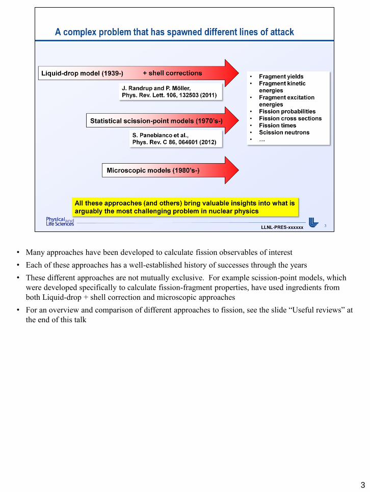
• Many approaches have been developed to calculate fission observables of interest

• Each of these approaches has a well-established history of successes through the years

• These different approaches are not mutually exclusive. For example scission-point models, which

were developed specifically to calculate fission-fragment properties, have used ingredients from

both Liquid-drop + shell correction and microscopic approaches

• For an overview and comparison of different approaches to fission, see the slide “Useful reviews” at

the end of this talk

3

• At the heart of the microscopic approach to fission is the self-consistent construction of the nuclear

Hamiltonian from effective (i.e., in-medium) interactions

• This type of approach began in the 50’s, with early attempts to understand and model the nuclear

force which led to the development of the first effective nuclear potentials (see, e.g., T.H.R. Skyrme,

Nucl. Phys. 9, 615 (1959))

• The idea is to relegate the phenomenological input (i.e., parameters that need to be adjusted to data)

to the effective interaction

• For nuclear properties calculated in a microscopic approach over the entire chart of the nuclei see,

e.g., S. Hilaire and M. Girod’s AMEDEE database:

http://www-

phynu.cea.fr/science_en_ligne/carte_potentiels_microscopiques/carte_potentiel_nucleaire_eng.htm

• For properties of even-even nuclei in particular see, e.g., J.-P. Delaroche et al., Nucl. Phys. A771,

103 (2006)

4

• One advantage of a microscopic approach is that the complexity of the quantum many-body

problem can be treated in stages, through a hierarchy of successive improvements

• The starting point is the mean-field description, where the individual nucleons only feel an average

potential, generated by the combination of all nucleons

• This pure mean field approach has been very successful in describing magic and near-magic nuclei

• The mean field is a coarse approximation, but it works well in magic nuclei because the residual

interaction (the part of the nucleon interaction that is not account for in the mean-field

approximation) is small compared to the energy of the first excited state. Thus, in magic nuclei, the

mean-field approximation gives a reasonably good description of the ground state

• Far from magicity (as will be the case for fission, in general) it may no longer be the case that the

residual interaction can be neglected compared to the excitation energy of low-lying states. In that

case, quantum mechanics couples the ground and excited states, and the residual interaction can no

longer be neglected

• Thus, we can follow a program of adding in the components of the residual interaction beyond the

mean field in order of importance

5

• For the fission problem, such a microscopic approach is appealing for a variety of reasons

• The fissioning nucleus explores a variety of exotic “shapes” that cannot be directly probed by

experimental measurements

• It also occurs in systems that are too short-lived to easily measure in the laboratory

• The parameters that enter into the microscopic approach (i.e., in the effective interaction) do not

need to be readjusted for different nuclei, different shapes, or different energies of those nuclei. In

particular, the same interaction can be used for the parent nucleus and its daughters

• Another appealing aspect of microscopic approaches is that collective motion (e.g., vibrations) are

built up from the underlying single-particle degrees of freedom. In this way, the single-particle and

collective motion are treated on an equal footing

• Furthermore, because the system is described by a Hamiltonian of interacting nucleons, quantum

mechanics can be built in from the start

• But, of course, there are major challenges in implementing such a program

6

• The first challenge we must contend with is that, despite the fact that great strides are being taken in

understanding the nucleon-nucleon interaction, we do not yet have a fundamental description of the

nuclear interaction (i.e., derived entirely from QCD)

• The problem is that QCD is non-perturbative in the low-energy regime of nuclear physics

• In any case, whatever nucleon-nucleon interaction we could derive from QCD would be modified

by complicated many-body effects inside the nucleus

• Thus, it makes more sense to use effective interaction, which are meant to capture the essential

features of the bare interaction modified by the nuclear medium

• For an introductory overview of current trends in research into effective nucleon-nucleon

interactions, see the course by D. Lacroix at

http://www.cenbg.in2p3.fr/heberge/EcoleJoliotCurie/coursannee/cours/D_lacroix.pdf

• For a more in-depth discussion see, e.g., E. Epelbaum et al., Rev. Mod. Phys. 81, 1773 (2009)

7

• For an introduction to the Brueckner-Goldstone expansion technique, see B. D. Day, Reviews of

Modern Physics 39, 719 (1967)

• See also M. de Llano, American Journal of Physics 38, 151 (1970) for a brief introduction to

effective interactions

• For a discussion of the formal connection between the theory of infinite nuclear matter and one type

of phenomenological interaction see J. W. Negele and D. Vautherin, Phys. Rev. C 5, 1472 (1972)

8

• Over the years, several functional forms have been used for these effective interactions

• One of the earliest, introduced by Skyrme, is the delta function

• The delta-function formulation has advantages (mathematical tractability) and disadvantages

(pathologies due to infinities)

• Skyrme interaction are still widely used for a variety of applications in nuclear physics, including

fission (see, e.g., J. McDonnell et al. in Proc. ICFN5, Sanibel Island FL (2012), p. 597, and

references therein)

• In order to avoid the pathologies associated with the delta function, D. Gogny introduced a (finite-

range) Gaussian form for the effective nucleon interaction. This is the form we will assume for the

rest of this lecture

9

• Like any effective interaction, the finite-range interaction has parameters that must be adjusted to

data

• In the traditional approach, those parameters are fitted to only a handful of nuclear data (namely

properties of infinite and semi-infinite nuclear matter), and measured properties of a few finite

nuclei

• More recent approaches have opted for a different strategy, fitting the parameters to a large number

of experimental data (e.g. nuclear masses: S. Goriely et al., Phys. Rev. Lett. 102, 242501 (2009))

• For this talk, we will assume the traditional approach of fitting very few data that are not a-priori

related to the fission observables of interest

10

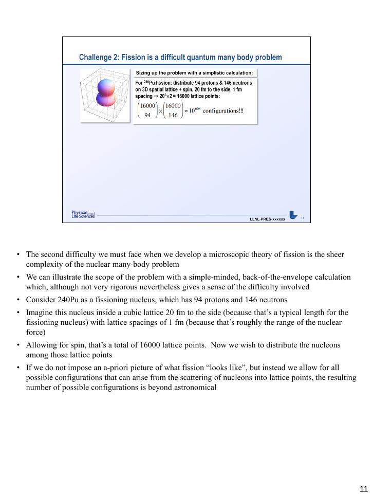
• The second difficulty we must face when we develop a microscopic theory of fission is the sheer

complexity of the nuclear many-body problem

• We can illustrate the scope of the problem with a simple-minded, back-of-the-envelope calculation

which, although not very rigorous nevertheless gives a sense of the difficulty involved

• Consider 240Pu as a fissioning nucleus, which has 94 protons and 146 neutrons

• Imagine this nucleus inside a cubic lattice 20 fm to the side (because that’s a typical length for the

fissioning nucleus) with lattice spacings of 1 fm (because that’s roughly the range of the nuclear

force)

• Allowing for spin, that’s a total of 16000 lattice points. Now we wish to distribute the nucleons

among those lattice points

• If we do not impose an a-priori picture of what fission “looks like”, but instead we allow for all

possible configurations that can arise from the scattering of nucleons into lattice points, the resulting

number of possible configurations is beyond astronomical

11

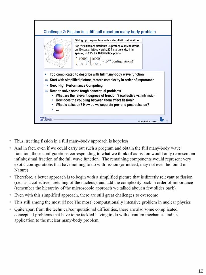
• Thus, treating fission in a full many-body approach is hopeless

• And in fact, even if we could carry out such a program and obtain the full many-body wave

function, those configurations corresponding to what we think of as fission would only represent an

infinitesimal fraction of the full wave function. The remaining components would represent very

exotic configurations that have nothing to do with fission (or indeed, may not even be found in

Nature)

• Therefore, a better approach is to begin with a simplified picture that is directly relevant to fission

(i.e., as a collective stretching of the nucleus), and add the complexity back in order of importance

(remember the hierarchy of the microscopic approach we talked about a few slides back)

• Even with this simplified approach, there are still great challenges to overcome

• This still among the most (if not The most) computationally intensive problem in nuclear physics

• Quite apart from the technical/computational difficulties, there are also some complicated

conceptual problems that have to be tackled having to do with quantum mechanics and its

application to the nuclear many-body problem

12

• Once again: since the full many-body wave function is too complicated, we have to start from a

simpler picture

• To put it in simple terms, the complication arises from the combinatorics of distributing many

nucleons among many states

• Traditionally, there are two main approaches to build this simple picture:

• The shell model, which reduces the number of states and nucleons that have to be considered

• The Hartree-Fock approximation, which replaces the full many-body wave function and its

enormous number of terms with a much simpler Slater determinant form

• Of course, this is an approximation, and the Slater determinant will never contain all the correlations

of the full wave function

• Furthermore, in order to describe the lowest states of the fissioning nucleus, we must find Slater

determinants that minimize the energy of the system (note that the Slater determinant that

minimizes the energy is not unique, we will have more to say on this later in the lecture)

• Finding a Slater determinant that minimizes the energy is usually done through an iterative

procedure that we will describe next

13

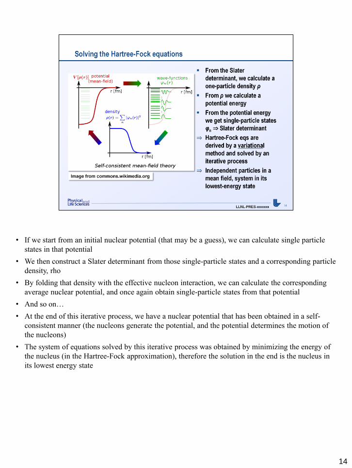
• If we start from an initial nuclear potential (that may be a guess), we can calculate single particle

states in that potential

• We then construct a Slater determinant from those single-particle states and a corresponding particle

density, rho

• By folding that density with the effective nucleon interaction, we can calculate the corresponding

average nuclear potential, and once again obtain single-particle states from that potential

• And so on…

• At the end of this iterative process, we have a nuclear potential that has been obtained in a self-

consistent manner (the nucleons generate the potential, and the potential determines the motion of

the nucleons)

• The system of equations solved by this iterative process was obtained by minimizing the energy of

the nucleus (in the Hartree-Fock approximation), therefore the solution in the end is the nucleus in

its lowest energy state

14

• The exchange term is present because of the anti-symmetrization of the overall wave function

15

• As we mentioned before, the Hartree-Fock approximation works best in magic nuclei, where the

residual interaction (beyond the mean field) is small compared to the energy of the first excited state

• For most nuclei, and for fission, this will not likely be a good approximation

• In particular, we know from experimental evidence that pairing plays an important role in the

structure and properties of most nuclei

• In order to include pairing correlations, we must go beyond the Hartree-Fock approximation. This

was done by M. Baranger, Phys. Rev. 122, 992 (1961), who generalized the Hartree-Fock method to

“Hartree-Fock-Bogoliubov” in order to take pairing into account

• In the microscopic approach, no additional parameters are required to describe pairing; is arises

from the sum of the effective interaction over correlated pairs of time-reversed states

16

• If we wish to consider subsets of the nucleus, the terms in the sum can be re-grouped to reflect the

contributions from the individual parts and their interactions

• This also means that the same effective interaction can be used for the parent nucleus from start to

scission, and for the daughters

• And the same applies to pairing of course

17

• So far the Hartree-Fock procedure we have described will always yield the state that is a (local)

minimum in energy

• But what if we are in the situation shown above, with a two-minimum potential. Which solution

will the Hartree-Fock procedure pick?

• The answer is that it depends on the starting point of the calculation (i.e., the initial potential or

initial Slater determinant that the iterative process starts from)

• For fission, we will need not just some local minima but the entire potential energy surface

• In order to explore that surface, we can introduce constraints through the method of Lagrange

multipliers

18

• Two commonly used constraints in the description of fission are the quadrupole and octupole

moments of the fissioning nucleus

• The quadrupole moment (roughly) controls the elongation of the nucleus as it stretches toward its

breaking points

• The octupole moment (roughly) controls the mass asymmetry of the nucleus, which eventually leads

to its division into a light and heavy fragment

19

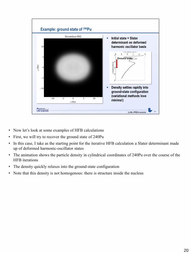
• Now let’s look at some examples of HFB calculations

• First, we will try to recover the ground state of 240Pu

• In this case, I take as the starting point for the iterative HFB calculation a Slater determinant made

up of deformed harmonic-oscillator states

• The animation shows the particle density in cylindrical coordinates of 240Pu over the course of the

HFB iterations

• The density quickly relaxes into the ground-state configuration

• Note that this density is not homogenous: there is structure inside the nucleus

20

• Next, we look at a solution far from the ground state, with a quadrupole moment of 200 barns

(compared to 28 for the ground state)

• Here, we need to introduce a constraint on Q20 to force the system to this deformation

• Normally such a calculation would be started from a nearby solution (e.g., one at Q20 = 196 barns),

but in order to demonstrate the robustness of the convergence in the HFB iterations, we start from

the ground-state solution obtained in the previous slide

• This time, more iterations are required, both because the starting point is far away, and because this

solution is not at a stable minimum of the system

• Note the mass asymmetry of the nuclear “shape” at the end. HFB has broken the right-left

symmetry that we began with, and we can start seeing a hint of what will become a light and a

heavy fragment

21

• Finally, let’s stretch the nucleus to its breaking point by imposing the constraint Q20 = 380 b

• Starting from the solution in the previous slide with Q20 = 200 b, this time it takes over 400

iterations to reach a fully converged result

• But, in this way, we can explore all configurations relevant to fission; from the ground state, out to

scission

22

• We see examples of collective motion in systems, built up from the simpler motion of its

constituents, at all scales in nature, for example:

• Murmuration of starlings (shown here)

• Flight of a swarm of bees

• Translational, rotational, vibrational, etc. motion can be decomposed into coherent sets of “single-

particle excitations”

• In a classical picture, the different collective configurations can then be assembled into a sequence

of frames which form a movie like the one shown here

23

• In quantum mechanics, all configurations exist at the same time, but each has its own weight

• This is the principle of quantum superposition

24

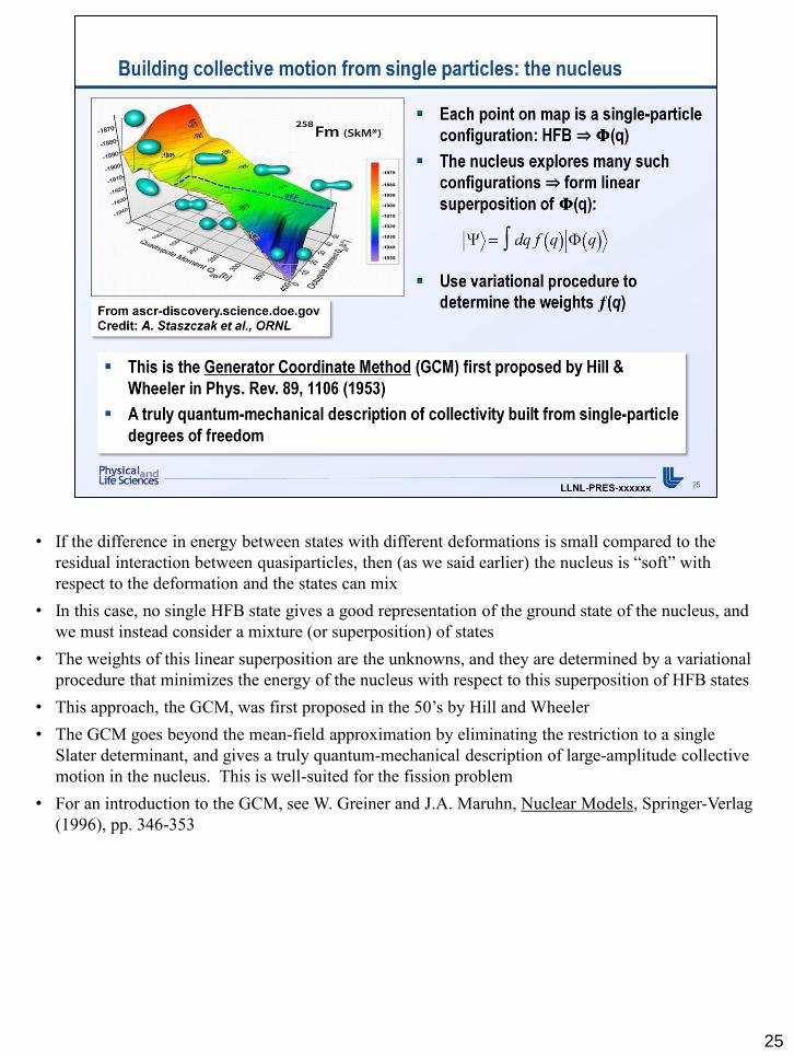
• If the difference in energy between states with different deformations is small compared to the

residual interaction between quasiparticles, then (as we said earlier) the nucleus is “soft” with

respect to the deformation and the states can mix

• In this case, no single HFB state gives a good representation of the ground state of the nucleus, and

we must instead consider a mixture (or superposition) of states

• The weights of this linear superposition are the unknowns, and they are determined by a variational

procedure that minimizes the energy of the nucleus with respect to this superposition of HFB states

• This approach, the GCM, was first proposed in the 50’s by Hill and Wheeler

• The GCM goes beyond the mean-field approximation by eliminating the restriction to a single

Slater determinant, and gives a truly quantum-mechanical description of large-amplitude collective

motion in the nucleus. This is well-suited for the fission problem

• For an introduction to the GCM, see W. Greiner and J.A. Maruhn, Nuclear Models, Springer-Verlag

(1996), pp. 346-353

25

• We illustrate the principle of the GCM with a simple example: the harmonic oscillator. This

example is discussed in more detail on p. 348 of W. Greiner and J.A. Maruhn, Nuclear Models,

Springer-Verlag (1996)

• In a variational approach, we would explore all possible values of the weights f(q) (and the complex

conjugate f*(q)) independently to find stationary points in the energy functional, as illustrated here

26

• Applying the variational principle with this new, configuration-mixing wave function leads to the

Hill-Wheeler (H-W) equation which involves integrals, derivatives, non-local and non-linear forms

• Note also that, in general, there is no reason to expect that HFB solutions at different deformations

will be orthogonal, hence we are left with norm overlaps <𝚿|𝚿>

• In principle, the H-W equation could be solved numerically, but this is a tremendous technical

challenge. In practice, the numerical solution of the full H-W equation has only been performed in

cases with limited number of constraints q (see for example P.H. Heenen, in the Joliot-Curie school

of 1991)

• We will take a different, more tractable approach here. Under certain conditions, the H-W equation

can be brought into the form of a Schrodinger-like equation. The first step is a change of

coordinates.

27

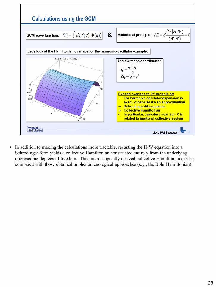
• In addition to making the calculations more tractable, recasting the H-W equation into a

Schrodinger form yields a collective Hamiltonian constructed entirely from the underlying

microscopic degrees of freedom. This microscopically derived collective Hamiltonian can be

compared with those obtained in phenomenological approaches (e.g., the Bohr Hamiltonian)

28

• We show here a calculation of the collective Schrodinger equation for 240Pu

• On the left, the potential energy term is shown along with the components of the inertia tensor

(since there are now two coordinates, these components introduce quadrupole-quadrupole,

quadrupole-octupole, and octupole-octupole couplings)

• On the right, we show results of the solution of the collective Schrodinger equation

• At the top right we show the spectrum of collective states obtained. Note that the second barrier has

been extrapolated to higher energies (dotted red line): this is done so that we can calculate quasi-

stationary vibrational states localized in the first and second wells (see for example, O. Serot et al.,

Nucl. Phys. A569, 562 (1994) for further discussion)

• The bottom right panel shows the wave function for one of the collective states near the top of the

barrier. Note how this wave function is localized in the second well.

29

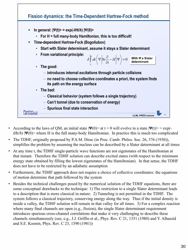
• According to the laws of QM, an initial state |𝝭(0)> at t = 0 will evolve to a state |𝝭(t)> = exp(-

iHt/) |𝝭(0)> where H is the full many-body Hamiltonian. In practice this is much too complicated

• The TDHF, originally proposed by P.A.M. Dirac (in Proc. Camb. Philos. Soc. 26, 376 (1930)),

simplifies the problem by assuming the nucleus can be described by a Slater determinant at all times

• At any time t, the TDHF single-particle wave functions are not eigenstates of the Hamiltonian at

that instant. Therefore the TDHF solution can describe excited states (with respect to the minimum

energy state obtained by filling the lowest eigenstates of the Hamiltonian). In that sense, the TDHF

does not have to be restricted by an adiabatic assumption

• Furthermore, the TDHF approach does not require a choice of collective coordinates: the equations

of motion determine that path followed by the system

• Besides the technical challenges posed by the numerical solution of the TDHF equations, there are

some conceptual drawbacks to the technique: 1) The restriction to a single Slater determinant leads

to a description that is more classical in nature. 2) Tunneling is not permitted in the TDHF. The

system follows a classical trajectory, conserving energy along the way. Thus if the initial density is

inside a valley, the TDHF solution will remain in that valley for all times. 3) For a complex reaction

where many final channels are open (e.g., fission), the single Slater determinant requirement

introduces spurious cross-channel correlations that make it very challenging to describe these

channels simultaneously (see, e.g., J.J. Griffin et al., Phys. Rev. C 21, 1351 (1980) and Y. Alhassid

and S.E. Koonin, Phys. Rev. C 23, 1590 (1981))

30

• Despite the difficulties, the TDHF has been used to gain a deeper understanding of fission dynamics

• The advantages of the TDHF mentioned previously (e.g., non-adiabatic features, automatically

determined fission path) make it an appealing tool for future research in fission

• For the purposes of this lecture, we will return instead to a time-dependent version of the GCM,

which avoids many of the difficulties of the TDHF approach by not limiting the wave function to a

single Slater determinant

31

• The GCM ansatz can be generalized so that the weights include a time dependence. Applying the

variational principle and expanding about the non-locality yields a time-dependent Schrodinger

equation in the collective coordinates. In the process, we recover again the collective Hamiltonian

that we obtained with the static GCM

• In order to solve this differential equation we need an initial condition, which is supplied by the

collective states calculated in the static GCM a few slides back

32

• The same microscopic ingredients (energy surface, inertia tensor) as in the static GCM calculations

enter into the calculation

• The result shown in the animation is a wave packet that evolves in time in the Q20-Q30 plane

toward the scission configurations

33

• So far, we have only considered collective modes in the fission calculations

• It is entirely possible that intrinsic (i.e., few quasiparticle) degrees of freedom can be excited as well

during the fission process. These intrinsic excitations are not normally considered in microscopic

fission calculations because of the technical complexity they introduce into the calculations

• From a conceptual point of view, the GCM can be readily extended to include such excitation with

respect to the HFB minima. Following the usual procedure (variation, expansion about the non-

locality) a generalized H-W equation is obtained that is no longer restricted to adiabatic conditions

• What is interpreted as dissipation in a semi-classical picture can now be described in a quantum-

mechanical framework as coupling between collective and intrinsic degrees of freedom

• This type of approach is currently in development. See the work of R. Bernard et al. and references

therein for further details

34

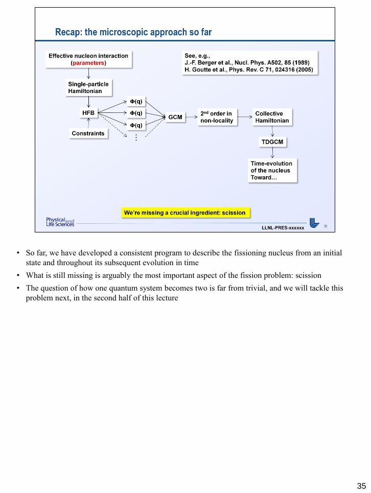
• So far, we have developed a consistent program to describe the fissioning nucleus from an initial

state and throughout its subsequent evolution in time

• What is still missing is arguably the most important aspect of the fission problem: scission

• The question of how one quantum system becomes two is far from trivial, and we will tackle this

problem next, in the second half of this lecture

35

36

• As a first step, let us consider scission from a geometrical perspective, by looking at the nucleon

density in the final stages of fission

• Although there may be some question about the exact point at which scission occurs, there is clearly

a “before” (first panel) and “after” (last panel)

• But in fact, this is an illusion…

37

• In quantum mechanics, geometric arguments based on the density can be misleading

• A better indicator of scission is the nuclear interaction energy between the two fragments. Since the

nuclear force has a very short range (~ 1 fm), we expect this interaction energy to quickly vanish as

the fragments move apart

• In a microscopic approach we can readily calculate this interaction energy without the need for any

new ingredients, and we find that the energy is far from negligible (compared, e.g., to the separation

energy of a nucleon, or ~ 6 MeV)

• In fact, this interaction energy never becomes negligible, even at relatively large separations

between the fragments

• If this is truly the case, then scission never really occurs…

38

• What is happening here is a beautiful manifestation of the non-local nature of quantum mechanics,

and another example of the richness of the microscopic approaches

• We can get a better picture of what is going on by plotting separately the densities of the left and

right fragments (to do this, we associate the single particle states whose wave functions are more

localized on the left fragment with that fragment, and likewise for the right fragment).

• On a log scale, we see that these single-particle states are not completely localized on their

respective fragment. Thus, each fragment has a tail extending into its complementary partner

• These tails may look small, but because they extend deeply into the heart of the complimentary

fragments, they can give rise to very large nuclear energies. In fact, our calculations show that each

particle in the tail contributes about an additional 50 MeV of binding energy between the fragments

39

• It is important to understand that this effect is not a consequence of any technical limitations in the

calculations (e.g., numerical accuracy or basis choice)

• It is well known for example that the solution of the Schrodinger equation for a double-well

potential in one dimension gives rise to delocalized orbitals. See for example the textbook by R.

Gilmore.

• In this example, we use square wells so that the solution can be written exactly and explicitly in

each region

• The question then is how do we define fission? And how do we recognize the pre-fragments

progressively, as we approach fission, so that we may extract their properties at scission?

• In the microscopic approach I have described so far, this is the central point:

• We use wave functions throughout

• We want to recognize the pre-fragments on those wave functions

40

• Here we simulate the pre-fragments moving apart before scission as the nucleus elongates by

separating the 1D wells

• Note that the tails disappear!

41

• As the parent nucleus evolves toward scission however, the potential wells of the pre-fragments also

change

• Here, we simulate this by making the well on the right progressively deeper

• As a consequence, single-particle levels move around, and can become degenerate in energy

• When a degeneracy occurs, the tails can reappear!

42

• The problem of delocalized orbitals is well-known in molecular physics.

• In addition, already in 1949, Sir Lennard-Jones had observed that orthogonal transformations of the

components of a Slater determinant leave all the properties of the system unchanged

• Based on this observation, molecular physicists use orthogonal transformations to recast the

delocalized electron orbitals produced in Hartree-Fock calculations into more physically meaningful

states that can be identified with, e.g., valence, bond, core orbitals (see, e.g., Jan H. Jensen,

“Molecular Modeling Basics” CRC Press (2010).)

• We can extend this concept to nuclear scission

• The HFB solution that is obtained by the usual variational procedure is not unique. In fact, any

unitary transformation of this solution will produce another with the same energy, same values of

the constraints, same global properties of the nucleus

• We illustrate this here using our simple 1D double-well example

43

• We have already noted that the very large nuclear interaction energies between the fragments was

caused by delocalized orbitals creating tails that extend into the complementary fragment

44

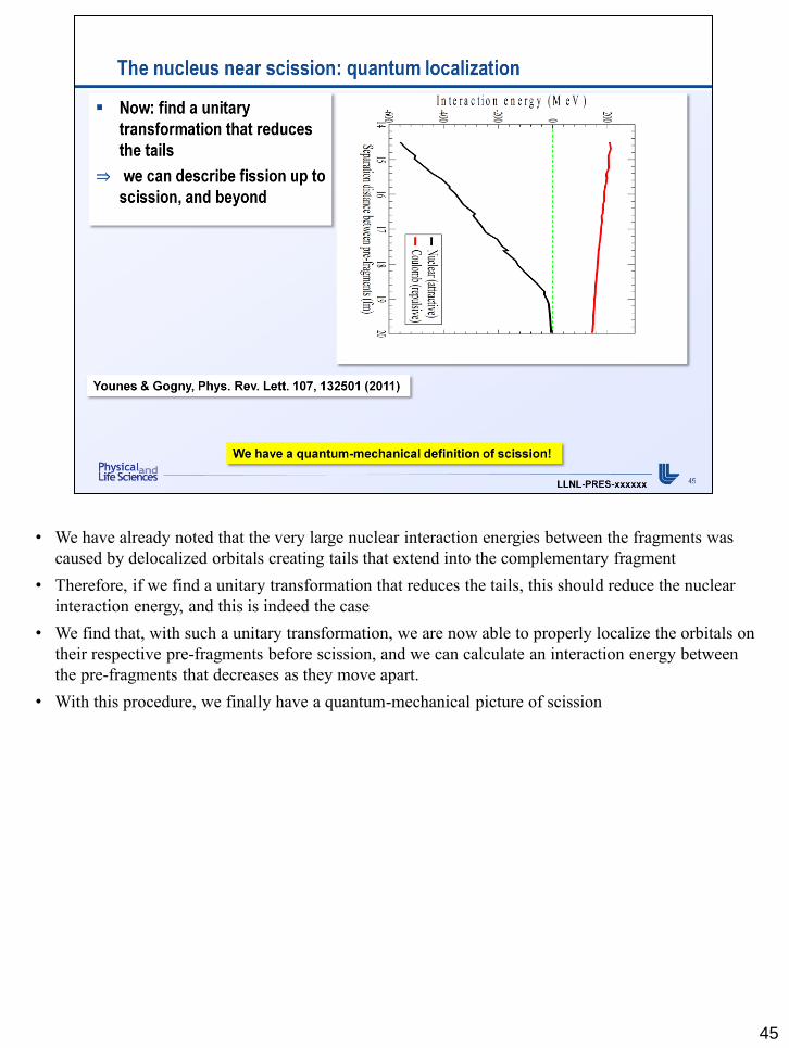
• We have already noted that the very large nuclear interaction energies between the fragments was

caused by delocalized orbitals creating tails that extend into the complementary fragment

• Therefore, if we find a unitary transformation that reduces the tails, this should reduce the nuclear

interaction energy, and this is indeed the case

• We find that, with such a unitary transformation, we are now able to properly localize the orbitals on

their respective pre-fragments before scission, and we can calculate an interaction energy between

the pre-fragments that decreases as they move apart.

• With this procedure, we finally have a quantum-mechanical picture of scission

45

• We are now in a position to give scission criteria that incorporate the non-local aspects of quantum

mechanics

• First, we expect at scission that the Coulomb force (which pushes the fragments apart) is much

larger than the nuclear force (which tries to keep them together). This criterion is commonly used in

other approaches, but in the microscopic approach, the forces are calculated in a consistent way

from a single effective interaction between the fragments

• As a second criterion, we require that the exchange energy (which is a purely quantum-mechanical

quantity) is small. This indicates that, to a good approximation, we can neglect the anti-

symmetrization between fragments

• Finally, we should be able to generate quasiparticle excitation localized on each fragment. To put it

another way, it should be possible to excite the individual fragments without destroying their

localization

• With these criteria verified, we can truly treat the fragments as separate entities

46

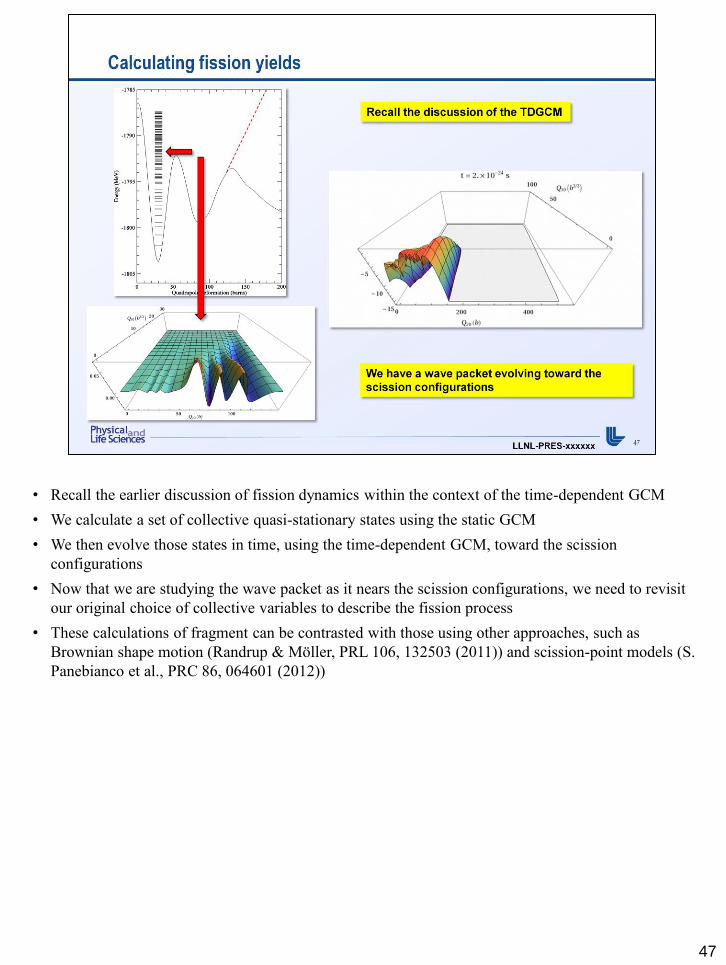
• Recall the earlier discussion of fission dynamics within the context of the time-dependent GCM

• We calculate a set of collective quasi-stationary states using the static GCM

• We then evolve those states in time, using the time-dependent GCM, toward the scission

configurations

• Now that we are studying the wave packet as it nears the scission configurations, we need to revisit

our original choice of collective variables to describe the fission process

• These calculations of fragment can be contrasted with those using other approaches, such as

Brownian shape motion (Randrup & Möller, PRL 106, 132503 (2011)) and scission-point models (S.

Panebianco et al., PRC 86, 064601 (2012))

47

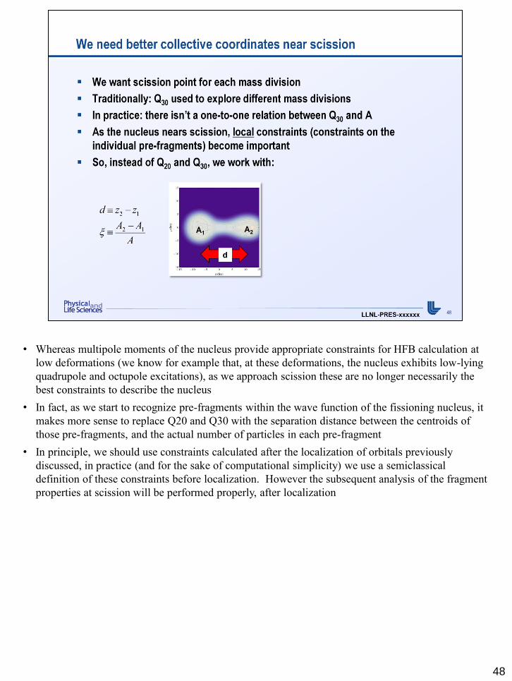
• Whereas multipole moments of the nucleus provide appropriate constraints for HFB calculation at

low deformations (we know for example that, at these deformations, the nucleus exhibits low-lying

quadrupole and octupole excitations), as we approach scission these are no longer necessarily the

best constraints to describe the nucleus

• In fact, as we start to recognize pre-fragments within the wave function of the fissioning nucleus, it

makes more sense to replace Q20 and Q30 with the separation distance between the centroids of

those pre-fragments, and the actual number of particles in each pre-fragment

• In principle, we should use constraints calculated after the localization of orbitals previously

discussed, in practice (and for the sake of computational simplicity) we use a semiclassical

definition of these constraints before localization. However the subsequent analysis of the fragment

properties at scission will be performed properly, after localization

48

• The scission configurations form a line in the 2D plane defined by the new coordinates

• This scission line defines a boundary between a region where we have one nucleus (the parent), and

two nuclei (the fragments)

• Note: with the new (d,AH) (or, equivalently, (d,ξ)) coordinates, we have scission points for each

mass division

49

• Here we show the probability current for an initial state at low energy (corresponding to thermal

fission)

• Note:

• very little flow for symmetric fission (A = 120)

• most of the flow is concentrated near most probable fission (A ~ 134 for heavy fragment and A ~

106 for light fragment)

• the flow is fairly slow

• From this current, a flux can be calculated all along the scission line. We interpret this flux as a

fission rate, and integrate it over time to get mass distributions for the fragments

50

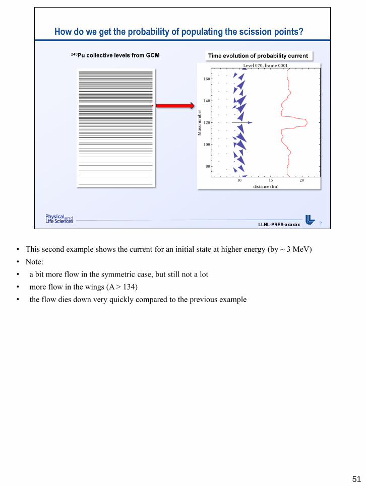
• This second example shows the current for an initial state at higher energy (by ~ 3 MeV)

• Note:

• a bit more flow in the symmetric case, but still not a lot

• more flow in the wings (A > 134)

• the flow dies down very quickly compared to the previous example

51

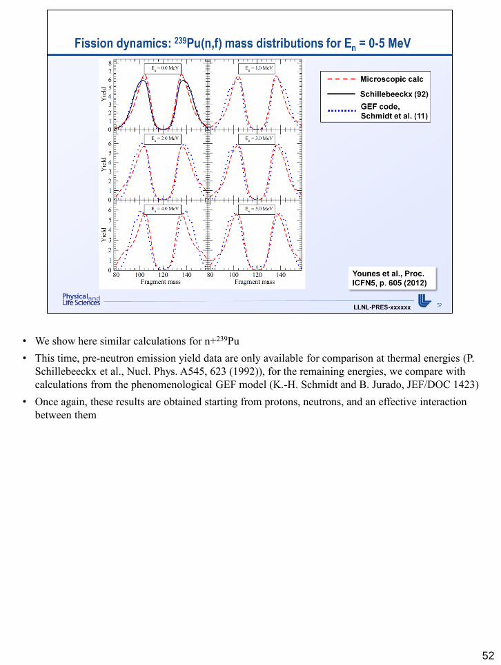
• We show here similar calculations for n+239Pu

• This time, pre-neutron emission yield data are only available for comparison at thermal energies (P.

Schillebeeckx et al., Nucl. Phys. A545, 623 (1992)), for the remaining energies, we compare with

calculations from the phenomenological GEF model (K.-H. Schmidt and B. Jurado, JEF/DOC 1423)

• Once again, these results are obtained starting from protons, neutrons, and an effective interaction

between them

52

• This is the same type of calculation, but this time for neutron on a 235U target, and as a function of

incident energy

• The different incident energies are obtained by starting from initial states at different excitation

energies

• In this case the calculations are compared to the pre-neutron mass distributions measured by Ch.

Straede et al., Nucl. Phys. A462, 85 (1987)

• Again, these results are obtained starting from protons, neutrons, and an effective interaction

between them

53

• We show here an example of the mass yield calculated for thermal neutron-induced fission on 229Th,

obtained by integrating the flux across the scission line

• The calculation (red) is compared to experimental data from Unik et al., in Proc. Int. Symp. On

physics and chemistry of fission, Rochester 1973 (IAEA, Vienna, 1973), vol II, p. 19

• Both experimental and calculated distributions represent yields before neutron emission

• It is worth remember that these results are obtained starting from protons, neutrons and an effective

interaction between them

54

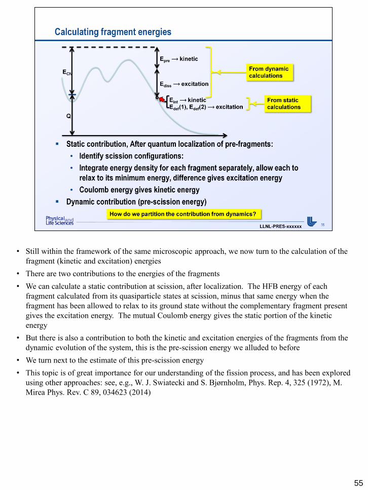
• Still within the framework of the same microscopic approach, we now turn to the calculation of the

fragment (kinetic and excitation) energies

• There are two contributions to the energies of the fragments

• We can calculate a static contribution at scission, after localization. The HFB energy of each

fragment calculated from its quasiparticle states at scission, minus that same energy when the

fragment has been allowed to relax to its ground state without the complementary fragment present

gives the excitation energy. The mutual Coulomb energy gives the static portion of the kinetic

energy

• But there is also a contribution to both the kinetic and excitation energies of the fragments from the

dynamic evolution of the system, this is the pre-scission energy we alluded to before

• We turn next to the estimate of this pre-scission energy

• This topic is of great importance for our understanding of the fission process, and has been explored

using other approaches: see, e.g., W. J. Swiatecki and S. Bjørnholm, Phys. Rep. 4, 325 (1972), M.

Mirea Phys. Rev. C 89, 034623 (2014)

55

• We will illustrate the dynamical effects on the energy with this simple example, and using the

collective Schrodinger equation derived from the GCM

• Note the transverse oscillations in the probability current

• not all the energy is in the direction of propagation

• we are interested in how the energy is partitioned between the two directions

56

• To illustrate this further, we can repeat the calculation with the same initial wave packet, but this

time eliminating anything that can give rise to motion in the transverse direction, i.e. we

• flatten out the potential surface

• set the component of the inertia tensor in the transverse direction to zero

• We refer to the resulting wave packet as the “1D wave” because it propagates essentially as if this

were a one-dimensional problem

• The original (unmodified) wave packet is referred to as the “2D wave”

• By plotting a cross-sectional cut of the 2D and 1D waves (note that both the real (blue) and

imaginary (red) parts of each wave are shown), we can see the effect of energy transfer to the

transverse motion which slows down the 2D wave relative to the 1D one. The question is: by how

much exactly?

57

• How can we quantify these observations?

• In principle, we could analyze the entire wave packet at each time step

• This becomes complicated when the wave packet is not a simple, well-localized function

• Instead, we will propose a method to extract the energy transferred to transverse motion from the

analysis at a single point (which we will call an “exit point”)

58

• To carry out this analysis, we use the WKB approximation, which lets us relate the normalized flux

of a wave packet to its energy

• The important point here is that if we observe a wave packet solution from the time-dependent

collective Schrodinger equation whose normalized flux is constant in time at an exit point, this

behavior suggests a solution that is a plane wave in the direction of propagation, and some other

function in the transverse direction. We never need to know this explicit form of the function in the

transverse direction because it cancels out in the calculation of the normalized flux!

59

• When we plot separately the flux in the direction of propagation and the squared amplitude at the

exit point as a function of time, we find very similar behaviors for both: both rise to a maximum as

the wave packet reaches them, and both fall away as it passes the exit point.

• The ratio of these two quantities (which gives the normalized flux) is relatively constant as long as a

significant portion of the wave packet is passing through the exit point

60

• We have described here a model to estimate the collective contribution to the pre-scission energy

(for more details see W. Younes & D. Gogny, LLNL-TR-586694 (2012))

• Note that we are still missing contributions from additional collective and intrinsic d.o.f.

• As a result, the present calculations should be taken as a lower bound (but probably not too low)

• The microscopic calculations of fragment energies can be contrasted with the phenomenological

models by Ruben et al. (Zeit. Phys. A 338, 67 (1991)) and Schmitt et al. (JEF/DOC 1423 (2011))

61

• For 239Pu(nth,f), the energy drop from saddle to scission for the most probable fission configuration

is about 15 MeV

• We have calculated an 8 MeV contribution to the kinetic energy after coupling with one collective

transverse mode. With additional coupling to intrinsic modes taking away a few more MeV, an

assumption of 50/50 split of the pre-scission energy between kinetic and excitation energies seems

reasonable.

• These quantities are consistent with other work using measured odd-even effects in fission products

to deduce dissipation, see e.g. Gönnenwein in Proceedings Phys. And Chem. of fission, Zfk-646

(1988), p. 13.

• The resulting calculations of the total kinetic (TKE) and total excitation (TXE) energies are

consistent with the data

• The TKE data shown here are taken from

• C. Wagemans et al., Phys. Rev. C 30, 218 (1984); K. Nishio et al., J. Nucl. Sci. Tech. 32, 404

(1995); C. Tsuchiya et al., J. Nucl. Sci. Tech. 37, 941 (2000)

• The TKE widths are from M. Asghar et al., Nucl. Phys. A311, 205 (1978)

• The TXE data are from J. Neiler et al., Phys. Rev. 149, 894 (1966)

62

• Even if more energy is dissipated into the excitation of the fragments through coupling with

additional transverse modes, the results are still consistent with the data!

63

• A similar calculation for the thermal fission of 235U also gives reasonable agreement with the data

• All this was, once again obtained, without invoking extraneous models. Note in particular that we

did not need to use statistical models or introduce a temperature to pump excitation energy into the

fragments

• TKE experimental data are taken from: H. W. Schmitt et al., Phys. Rev. 141, 1146 (1966); P.P.

Dyachenko et al., Phys. Lett. B 31, 122 (1970); H. Baba et al., J. Nucl. Sci. Tech. 34, 871 (1997)

• TXE experimental data are from H. W. Schmitt et al., Phys. Rev. 141, 1146 (1966)

64

• A similar calculation for the thermal fission of 229Th also gives reasonable agreement with the data

• All this was, once again obtained, without invoking extraneous models. Note in particular that we

did not need to use statistical models or introduce a temperature to pump excitation energy into the

fragments

• TKE data are from M. Asghar et al., Nucl. Phys. A373, 225 (1982)

• TXE data were obtained from Q values and TKE

65

66

67

68

• In closing, we mention other work on various aspects of the fission process using microscopic

approaches.

• This is by no means an exhaustive list, either in topic or in authors. It is only intended to show that

there is extensive ongoing work on fission beyond what I have time to cover in this lecture

69

70

71