Appendix

The Stress Circle

O. Mohr’s stress circle diagram is an extremely useful geometrical representation of thestate of stress at a point. It is particularly convenient in problems of plane deformation,since the state of stress may then be visualized by a single stress circle.

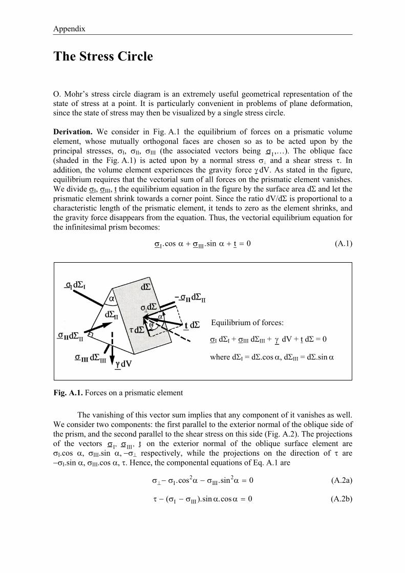
Derivation. We consider in Fig. A.1 the equilibrium of forces on a prismatic volumeelement, whose mutually orthogonal faces are chosen so as to be acted upon by theprincipal stresses, I, II, III (the associated vectors being ,…). The oblique face(shaded in the Fig. A.1) is acted upon by a normal stress and a shear stress . Inaddition, the volume element experiences the gravity force dV. As stated in the figure,equilibrium requires that the vectorial sum of all forces on the prismatic element vanishes.We divide I, III, t the equilibrium equation in the figure by the surface area d and let theprismatic element shrink towards a corner point. Since the ratio dV/d is proportional to acharacteristic length of the prismatic element, it tends to zero as the element shrinks, andthe gravity force disappears from the equation. Thus, the vectorial equilibrium equation forthe infinitesimal prism becomes:

I III.cos .sin t 0 (A.1)

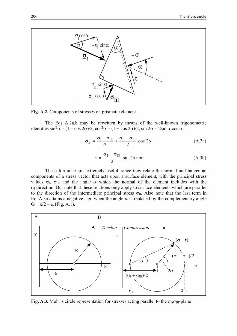
The vanishing of this vector sum implies that any component of it vanishes as well.We consider two components: the first parallel to the exterior normal of the oblique side ofthe prism, and the second parallel to the shear stress on this side (Fig. A.2). The projectionsof the vectors , , t on the exterior normal of the oblique surface element are

I.cos , III.sin respectively, while the projections on the direction of areI.sin , III.cos , . Hence, the componental equations of Eq. A.1 are

2 2III.cos .sin 0 (A.2a)

I III( ).sin .cos 0 (A.2b)

Equilibrium of forces:

I d + III d + dV + t d = 0

where d = d .cos , d III = d .sin

Fig. A.1. Forces on a prismatic element

206 The stress circle

Fig. A.2. Components of stresses on prismatic element

The Eqs. A.2a,b may be rewritten by means of the well-known trigonometricidentities sin2 = (1 – cos 2 )/2, cos2 = (1 + cos 2 )/2, sin 2 = 2sin .cos :

I III I III .cos 22 2

(A.3a)

I III .sin 22

(A.3b)

These formulae are extremely useful, since they relate the normal and tangentialcomponents of a stress vector that acts upon a surface element, with the principal stressvalues I, III and the angle which the normal of the element includes with the

I direction. But note that these relations only apply to surface elements which are parallelto the direction of the intermediate principal stress II. Also note that the last term inEq. A.3a attains a negative sign when the angle is replaced by the complementary angle

/2 – (Fig. A.1).

Fig. A.3. Mohr’s circle representation for stresses acting parallel to the I, III-plane

a

R

x

y

A

( I III)/ 2

( I III)/ 2

I III

2

CompressionTension

B

The stress circle 207

The angle can be eliminated from the Eqs. A.3a,b. Because ofsin2 2 + cos2 2 = 1, rearranging terms in the equations, squaring and adding yields

2 22I III I III

2 2(A.4)

Mohr’s stress circle. If we compare Eq. A.4 with the equation

2 2 2x a y R

of a circle in a Cartesian x,y-coordinate system (Fig. A.3A), we notice immediately thatEq. A.4 represents a circle in a two-dimensional Cartesian frame with the coordinates

and (Fig. A.3B).The “stress circle” has the radius ( I – III)/2, intersects the -axis at the points

( III,0) and ( I,0), and is centred on the -axis at a distance of ( I + III)/2 from the origin.The coordinates , of a point on the circle represent the normal and tangential stresscomponents of the stress vector t which acts on a planar element which is parallel to theintermediate principal stress II. Since we count compressive stresses as positive, thecorresponding stress points will lie in the positive half-plane of the diagram.

It is important to note that the radius vector to a stress point, associated with aplanar element whose normal includes the angle with the I direction (Fig. A.2), includestwice that angle with the -axis. The corresponding relation tan 2 = /[ – ( I + III)/2]in Fig. A.3B follows directly from the parameter equations (Eqs. A.3a,b) of the stresscircle. Needless to say, is not only the angle between the normals of two planar elements,but also the angle included by the elements themselves. Hence, when a planar element inreal space is rotated anticlockwise around the II-axis through an angle , the radiusvector of the stress circle is rotated through 2 .

Note also that the chord extending from the stress point ( III,0) to a stress point( , ) makes the angle with the -axis, since according to an elementary geometricaltheorem the angle extended from any point on the periphery of a circle over a given arc ofthe circle amounts to half the angle extended over the same arc from the center of thecircle.

Fig. A.4. Maximum shear stress in the Mohr diagram

)( / 2+

- )( /2max| | =max

max

45°

45°

208 Stress relations

The Mohr circle is fully determined and easily constructed when the principal stressvalues I and III are prescribed, or when the normal and shear stresses that act on twoarbitrary, mutually orthogonal planes, are known, in which case the associated stress pointslie at the opposite ends of a diameter of the circle.

Maximum shear stress. From the Mohr Diagram (Fig. A.4) it is immediatelyapparent that maximum shear stresses max occur on elements inclined at 45° to the I-axis(i.e. 2 = 90°) since = 0 for the radius vector to the principal stress point ( I,0). Thenormal stress acting on these elements is ( I + III)/2, while max = ±( I – III)/2. The twomaximum shear stresses are equal in magnitude, as is required by the symmetricorientation of the two elements with respect to the I-axis.

Stress relations. If the normal and shear stresses that act upon two mutually perpendicularplanes which are parallel to the II direction are known, the values of the principal stresses

I, III and the maximal shear stress max can be read from the Mohr Circle. These stressesmay be also determined from the analytical expressions:

which are derived by applying Pythagoras’ Theorem to the shaded triangles in Fig. A.5A.Similarly, the directions of the principal stresses I and III are easily determined

with respect to a material element whose normal and shear stress are known. For the simpleconstruction in the Mohr Diagram in Fig. A.5B the material reference element was chosenwith the normal parallel to the x3-axis of a Cartesian system (see insert of Fig. A.5B). Theelement is acted upon by the stresses 3 and 31. Hence, the radius vector to the point( 3, 31) on the stress circle includes the angle 2 with the radius vector to the point I,0),i.e., twice the angle between the I-axis and the x3-axis in real space. The complementaryangle 2 in the Mohr Diagram is then twice the angle between the I axis and the x1-axis.The shaded right-angled triangle in Fig. A.5B immediately provides the importantanalytical expression for the orientation of the I-axis:

311 3

2tan 2 tan 2 ( ) (A.6)

where 1 and 3 are the normal stresses that act upon the elements with normals parallel tothe x1- and x3-axes of a Cartesian frame, and 31 = 13 is the shear stress on theseelements.

Note that the roles of the x1- and the x3-axes in Eq. A.6 are interchanged, if 1 < 3,and the angle * in tan 2 * = 2 / 3 – 1) becomes the angle between the I-axis and thex3-axis.

Three-dimensional state of stress. So far, we have dealt with stresses that act uponmaterial elements whose normals are perpendicular to the II-axis Although we shall

maxI III

21 3

2

4 132

1 32

1 32

4 132

I

III

(A.5a)

(A.5b)

Stress relations 209

mostly deal with this type of elements, occasionally we may also consider elements withnormals perpendicular to the I-axis or to the III-axis. The stresses of these elements mapon one of the smaller circles in Fig. A.6. Without proof, we add that the stresses ,which act on elements that are obliquely oriented with respect to all three principal stressdirections map on the interior of the crescent-shaped region enclosed by the three principalstress circles.

x• •

•

•3,

1,-

IIII

1 3

1 3

1

> 0

> 03

x1

x

3

x• •1

IIII

• •

1 3-_____2

•

III

x1

I

I

III

x

Fig. A.5. Stress relations in the Mohr Diagram:A) principle stresses and Cartesian stress components;B) orientation of principal axes in Cartesian reference frame (see text)

210 The “pole” of the stress circle

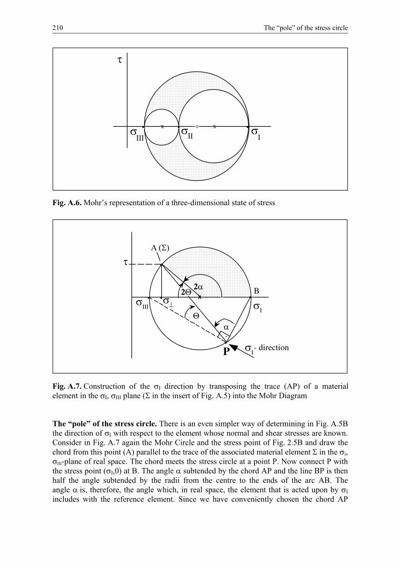
Fig. A.6. Mohr’s representation of a three-dimensional state of stress

Fig. A.7. Construction of the I direction by transposing the trace (AP) of a materialelement in the I, III plane ( in the insert of Fig. A.5) into the Mohr Diagram

The “pole” of the stress circle. There is an even simpler way of determining in Fig. A.5Bthe direction of I with respect to the element whose normal and shear stresses are known.Consider in Fig. A.7 again the Mohr Circle and the stress point of Fig. 2.5B and draw thechord from this point (A) parallel to the trace of the associated material element in the I,

III-plane of real space. The chord meets the stress circle at a point P. Now connect P withthe stress point ( I,0) at B. The angle subtended by the chord AP and the line BP is thenhalf the angle subtended by the radii from the centre to the ends of the arc AB. Theangle is, therefore, the angle which, in real space, the element that is acted upon by Iincludes with the reference element. Since we have conveniently chosen the chord AP

•• •x x°

• •

IIII

•

•

•P I

- direction

x2

2 B

The “pole” of the stress circle 211

parallel to the trace of the reference element in the I, III-plane, the line segment BP isalso parallel to the trace of the element acted upon by the maximum principal stress I.Since I acts perpendicularly on this element, the I-axis is parallel to the chord drawnfrom the point ( III,0) to P.

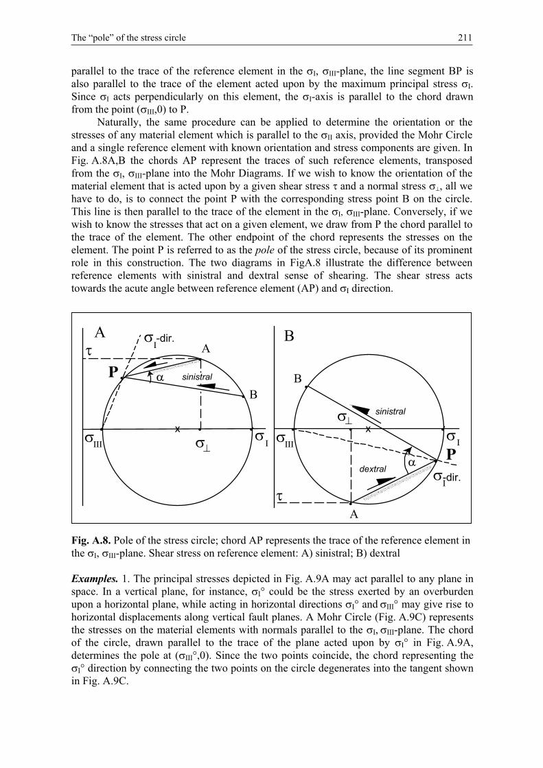
Naturally, the same procedure can be applied to determine the orientation or thestresses of any material element which is parallel to the II axis, provided the Mohr Circleand a single reference element with known orientation and stress components are given. InFig. A.8A,B the chords AP represent the traces of such reference elements, transposedfrom the I, III-plane into the Mohr Diagrams. If we wish to know the orientation of thematerial element that is acted upon by a given shear stress and a normal stress , all wehave to do, is to connect the point P with the corresponding stress point B on the circle.This line is then parallel to the trace of the element in the I, III-plane. Conversely, if wewish to know the stresses that act on a given element, we draw from P the chord parallel tothe trace of the element. The other endpoint of the chord represents the stresses on theelement. The point P is referred to as the pole of the stress circle, because of its prominentrole in this construction. The two diagrams in FigA.8 illustrate the difference betweenreference elements with sinistral and dextral sense of shearing. The shear stress actstowards the acute angle between reference element (AP) and I direction.

Fig. A.8. Pole of the stress circle; chord AP represents the trace of the reference element inthe I, III-plane. Shear stress on reference element: A) sinistral; B) dextral

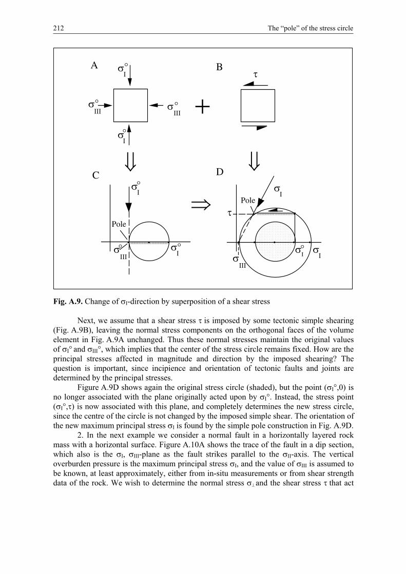
Examples. 1. The principal stresses depicted in Fig. A.9A may act parallel to any plane inspace. In a vertical plane, for instance, I° could be the stress exerted by an overburdenupon a horizontal plane, while acting in horizontal directions ° and III° may give rise tohorizontal displacements along vertical fault planes. A Mohr Circle (Fig. A.9C) representsthe stresses on the material elements with normals parallel to the , III-plane. The chordof the circle, drawn parallel to the trace of the plane acted upon by ° in Fig. A.9A,determines the pole at ( III°,0). Since the two points coincide, the chord representing the

° direction by connecting the two points on the circle degenerates into the tangent shownin Fig. A.9C.

3

x• •IIII

•

•

•P

•

I-dir.

sinistral

3

x• •IIII

•

•

• P

•

I-dir.

sinistral

dextral

212 The “pole” of the stress circle

Fig. A.9. Change of I-direction by superposition of a shear stress

Next, we assume that a shear stress is imposed by some tectonic simple shearing(Fig. A.9B), leaving the normal stress components on the orthogonal faces of the volumeelement in Fig. A.9A unchanged. Thus these normal stresses maintain the original valuesof I° and III°, which implies that the center of the stress circle remains fixed. How are theprincipal stresses affected in magnitude and direction by the imposed shearing? Thequestion is important, since incipience and orientation of tectonic faults and joints aredetermined by the principal stresses.

Figure A.9D shows again the original stress circle (shaded), but the point ( I°,0) isno longer associated with the plane originally acted upon by I°. Instead, the stress point( I°, ) is now associated with this plane, and completely determines the new stress circle,since the centre of the circle is not changed by the imposed simple shear. The orientation ofthe new maximum principal stress I is found by the simple pole construction in Fig. A.9D.

2. In the next example we consider a normal fault in a horizontally layered rockmass with a horizontal surface. Figure A.10A shows the trace of the fault in a dip section,which also is the I, III-plane as the fault strikes parallel to the II-axis. The verticaloverburden pressure is the maximum principal stress I, and the value of III is assumed tobe known, at least approximately, either from in-situ measurements or from shear strengthdata of the rock. We wish to determine the normal stress and the shear stress that act

• ••

Pole

Pole

• ••

•

••

•

A B

C D

°

°

°

°

°°

° °I

The “pole” of the stress circle 213

upon the fault plane. With I and III being known, we can draw the stress circle inFig. A.10B. As in the preceding example, the point ( III,0) becomes again the pole, fromwhich we draw the chord parallel to the fault trace in Fig. A.10A. The coordinates of thepoint where the chord meets the circle represent the normal and tangential stresscomponents on the fault.

Fig. A.10. Normal and shear stress on a normal fault in a horizontally layered rock mass:A) dip section of the fault with principal stresses;B) determination of fault stresses in the Mohr diagram

normalfault •

•

POLE

•

fault plane

References

Ashby MF, Hallam SD (1986) The failure of brittle solids containing small cracks under compressivestress states. Acta metallurgy 34:497–510

Atkinson BK (1987) Fracture mechanics of rocks. Academic Press, LondonBai T, Pollard DD (2000) Closely spaced fractures in layered rocks: initiation mechanism and

propagation kinematics. J Struct Geol 22:1409–1425Bankwitz P, Bahat D, Bankwitz E (2000) Granitklüftung – Kenntnisstand 80 Jahre nach Hans Cloos.

Z Geol Wiss 28(1/2):87–110Barquins M, Petit J-P (1992) Kinetic instabilities during the propagation of a branch crack: effects of

loading conditions and internal pressure. J Struct Geol 14:893–903Beach A (1977) Vein arrays, hydraulic fractures and pressure solution structures in a deformed flysch

sequence, SW England. Tectonophysics 40:201–225Bock H (1980) Die Rolle der Werkstoffkunde bei der mechanischen Interpretation geologischer

Trennflächen. N Jb Geol Paläont Abh 160:380–405Bourne SJ, Willemse EJM (2001) Elastic stress control on the pattern of tensile fracturing around a

small fault network at Nash Point, UK. J Struct Geol 23:1753–1770Brace WF, Bombolakis EG (1963) A note on brittle crack growth in compression. J Geophys Res

68(12):3709–3713Cooke ML, Underwood CA (2001) Fracture termination and step-over at bedding interfaces due to

frictional slip and interface opening. J Struct Geol 23:223–238Cotterell B, Rice JR (1980) Slightly curved or kinked cracks. Int J Fracture 16:155–169Cundall P (1990) Numerical modelling of jointed and faulted rock. In: Rossmanith HP (ed) Proceedings

of the International Conference on the Mechanics of Jointed and Faulted Rock, Vienna, Austria.Balkema, Rotterdam, pp 11–18

Dyer R (1988) Using joint interactions to estimate paleostress ratios. J Struct Geol 10:685–699Engelder T (1987) Joints and shear fractures in rock. In: Atkinson BK (ed) Fracture Mechanics of

Rocks. Academic Press, London, pp 27–69Engelder T (1993) Stress regimes in the lithosphere. Princeton University PressFriedman M (1972) Residual elastic strain in rocks. Tectonophysics 15:297–330Friedman M, Logan JM (1970) Influence of residual elastic strain on the orientation of experimental

fractures in three quartzose sandstones. J Geophys Res 75(2):387–405Gramberg J (1989) A non-conventional view on rock mechanics and fracture mechanics. Balkema,

RotterdamGretener PE (1983) Remarks by a geologist on the propagation and containment of extension fractures.

Bull Ver Schweiz Petroleum-Geol Ing 49(116):29–35Griffith AA (1925) Theory of rupture. In: Proc. 1st Int. Congress Appl. Mechanics, Delft. J. Waltman,

Delft, pp 55–63Gross MR (1993) The origin and spacing of cross joints: examples from the Monterey Formation, Santa

Barbara coastline, California. J Struct Geol 15:737–751Hallbauer DK, Wagner H, Cook NGW (1973) Some observations concerning the microscopic and

mechanical behaviour of quartzite specimens in stiff, triaxial compression tests. Int J RockMech Min Sci 10:713–726

Helgeson DE, Aydin A (1991) Characteristics of joint propagation across layer interfaces insedimentary rocks. J Struct Geol 13:897–911

Hobbs DW (1967) The formation of tension joints in sedimentary rocks: an explanation. Geol Magazine104:550–556

Hoek E, Bieniawski ZT (1965) Brittle fracture propagation in rock under compression. Int J Rock MechMin Sci 1:137–155

Holzhausen GR, Johnson AM (1979) Analysis of longitudinal splitting of uniaxially compressed rockcylinders. Int J Rock mech Min Sci 16:163–177

Josselin de Jong G (1959) Statics and kinematics in the failable zone of granular material. Dr. thesis,Techn. University Delft

Kármán von T (1911) Festigkeitsversuche unter allseitigem Druck. Z Ver dt Ing 55:1749–57

216 References

Kemeny JM (1993) The micromechanics of deformation and failure in rocks. In: Pasamehmetoglu et al.(eds) Assessing and Prevention of Failure Phenomena in Rock Engineering, Balkema,Rotterdam, pp 23–33

King G, Sammis C (1992) The Mechanisms of finite brittle strain. Pageoph 138(4):611–640Lachenbruch AH (1961) Depth and spacing of tension cracks. J Geophys Res 66:4273–4292Lachenbruch AH (1962) Mechanics of thermal contraction cracks and ice-wedge polygons in

permafrost. Geological Society of America Special Paper 70Lagalli M (1930) Versuch einer Theorie der Spaltenbildung in Gletschern. Z Gletscherkunde 17:285–301Lawn BR, Wilshaw TR (1975) Fracture of brittle solids. Cambridge University PressLehner F, Pilaar WF (1974) Shell Research Report (internal)Lehner F, Pilaar WF (1997) The emplacement of clay smears in syn-sedimentary normal faults:

inference from field observations near Frechen, Germany. In: Moller-Pedersen P, Koestler AG(eds) Hydrocarbon seals. Norwegian Petroleum Soc Special Publ 7:39–50

Leroy Y, Ortiz M (1990) Finite-element analysis of transient strain localization phenomena in frictionalsolids. Int J Numer Anal Met Geomech 14:93–124

Lockner DA, Madden TR (1991) A multiple-crack model of brittle fracture, II. Time-dependentsimulations. J Geophys Res 96:19643–19654

Mandl G (1987a) Tectonic deformation by rotating parallel faults: the “bookshelf” mechanism.Tectonophysics 141:277–316

Mandl G (1987b) Discontinuous fault zones. J Struct Geol 9:105–110Mandl G (1988) Mechanics of tectonic faulting, models and basic concepts. Elsevier, AmsterdamMandl G (2000) Faulting in brittle rocks: an introduction to the mechanics of tectonic faults. Springer-

Verlag, Heidelberg BerlinMandl G, Harkness R (1987) Hydrocarbon migration by hydraulic fracturing. In: Jones ME, Preston

RMF (eds) Deformation of sediments and sedimentary rocks. Geol Soc Specail Publ 29:39–53Martel SJ (1990) Formation of compound strike-slip fault zones, Mount Abbot quadrangle, California.

J Struct Geol 12:869–882McGarr A (1980) Some constraints on levels of shear stress in the crust from observations and theory.

J Geophys Res 85:6231–6238McQuillan H (1973) Small-scale fracture density in Asmari Formation of southwest Iran and its relation

to bed thickness and structural setting. Am Assoc Petrol Geol Bull 57:2367–2385Meier D, Kronberg P (1989) Klüftung in Sedimentgesteinen. Enke, StuttgartMollema PN, Antonellini M (1999) Development of strike-slip faults in the dolomites of the Sella

Group, Northern Italy. J Struct Geol 21:273–292Moore DE, Summers R, Byerlee JD (1990) Deformation of granite during triaxial friction tests. In:

Rossmanith HP (ed) Proceedings of the International Conference on the Mechanics of Jointedand Faulted Rock, Vienna, Austria. Balkema, Rotterdam, pp 345–352

Narr W, Suppe J (1991) Joint spacing in sedimentary rocks. J Structl Geol 13(9):1037–1048Nur A (1982) The origin of tensile fracture lineaments. J Struct Geol 4(1):31–40Olson JE, Pollard DD (1991) The initiation and growth of en échelon veins. J Struct Geol 13(5):

595–608Petit J-P, Barquins M (1988) Can natural faults propagate under mode II conditions? Tectonics 7:

1243–1256Petit J-P, Auzias V, Rawnsley KD, Rives T (2000) Development of joint sets in the vicinity of faults. In:

Lehner FK, Urai JL (eds) Aspects of Tectonic Faulting. Springer-Verlag, Berlin Heidelberg,pp 167–183

Poliakov ANB, Herrmann HJ, Podladchikov YY, Roux S (1994) Fractal plastic shear bands. Fractals2(4):567–581

Pollard DD (1973) Derivation and evaluation of a mechanical model for sheet intrusion. Tectonophysics19:233–269

Pollard DD, Aydin A (1988) Progress in understanding jointing over the past century. Geol Soc AmBull 100:1181–1204

Pollard DD, Müller O (1976) The effect of gradients in regional stress and magma pressure on the formof sheet intrusions in cross section. Geophys Res Letters 81(5):975–988

Pollard DD, Segall P (1987) Theoretical displacements and stresses near fractures in rocks: withapplications to faults, joints, veins, dikes, and solution surfaces. In: Atkinson BK (ed) Fracturemechanics of rocks. Academic Press, London, pp 277–349

References 217

Pollard DD, Segall P, Delaney PT (1982) Formation and interpretation of dilatant echelon cracks. GeolSoc Am Bull 93:1291–1303

Price NJ (1966) Fault and joint development in brittle and semi-brittle rock. Pergamon Press, OxfordPrice NJ (1974) The development of stress systems and fracture patterns in undeformed sediments.

Proceedings of the 3rd Congress of the International Society for Rock Mechanics, Denver,Colorado, pp 487–496

Price NJ, Cosgrove JW (1990) Analysis of geological structures. Cambridge University PressRamsay JG (1980) The crack-seal mechanism of rock deformation. Nature 284:135–139Ramsay JG, Huber M (1987) The techniques of modern structural geology, vol. 2: Folds and fractures.

Academic Press, LondonRawnsley KD, Rives T, Petit J-P, Hencher SR, Lumsden AC (1992) Joint perturbations at faults.

J Struct Geol 14(8/9):939–951Renshaw CE, Pollard DD (1994) Are large differential stresses required for straight fracture propagation

paths? J Struct Geol 16:817–822Rives T, Petit J-P (1990) Experimental study of jointing during cylindrical and non-cylindical folding.

In: Rossmanith HP (ed) Proceedings of the International Conference on the Mechanics ofJointed and Faulted Rock, Vienna, Austria. Balkema, Rotterdam, pp 205–211

Rossmanith HP (1990) Mechanics of jointed and faulted rock: Proceedings of an InternationalConference, Vienna, Austria. Balkema, Rotterdam

Rudnicki JW, Rice JR (1975) Conditions for the localization of deformation in pressure-sensitivedilatant materials. J Mech Phys Solids 23:371–394

Secor DT Jr., Pollard DD (1975) On the stability of open hydraulic fractures in the Earth’s crust.Geophys Res Letters 2(11):510–513

Segall P, Pollard DD (1983) Nucleation and growth of strike-slip faults in granite. J Geophys Res88(B1):555–568

Sibson RH (1981) Controls on low-stress hydro-fracture dilatancy in thrust, wrench and normal faultterrains. Nature 289:665–667

Sobolev G, Spetzler H, Salov B (1978) Precursors to failure in rocks while undergoing anelasticdeformations. J Geophys Res 83(B4):1775–1784

Suppe J (1985) Principles of structural geology. Prentice Hall, LondonTakada A (1990) Experimental study on propagation of liquid-filled crack in gelatin: shape and velocity

in hydrostatic stress condition. J Geophys Res 95:8471–8481Tatsuoka F, Nakamura S, Huang C-C, Tani K (1990) Strength anisotropy and shear band direction in

plane strain tests on sand. Soils and Foundations 30(1):35–54Terzaghi K (1923) Die Berechnung der Durchlässigkeitsziffer des Tones aus dem Verlauf der

hydrodynamischen Spannungserscheinungen. Sitzungsberichte der Akademie derWissenschaften Wien, mathematisch-naturwissenschaftliche Klasse 132(11a):107–122

Terzaghi K (1925) Erdbaumechanik auf bodenphysikalischer Grundlage. Deutike, WienThomas A L, Pollard DD (1993) The geometry of echelon fractures in rock: implications from

laboratory and numerical experiments. J Struct Geology 15:323–334Vermeer PA (1990) The orientation of shear bands in biaxial tests. Géotechnique 40(2):223–236Vermeer PA, de Borst R (1984) Non-associated plasticity for soils, concrete, and rock. Heron 29:1–64Vutukuri VS, Lama RD, Saluja SS (1974) Handbook on mechanical properties of rocks, vol I.

Transtech Publications, ClausthalWeertman J (1971) Theory of water-filled crevasses in glaciers applied to magma transport beneath

oceanic ridges. J Geophys Res 76:1171–1183

Index

Symbols

-factor 28, 29-factor 30

A

aperture (see hydraulic fracture)

B

basin–, Earth’s curvature 109–, exfoliation 116, 117–, joint parallel to

–, long axis 111–113–, short axis 116

–, reference model 106, 123–, residual stress 116–, subsidence 109–113

–, overpressuring 111–, uplift 105–108

“bookshelf” mechanism–, dilational style 143, 150, 174, 188, 191–, domino style 142

brittle–, definition 5–8

–, vs. ductile 8, 9–, semi-brittle 8

C

cap rock (migration through) 30–43, 46capillary entry pressure 45cleavage fracture (axial splitting) (see extension

fracture)crack-seal mechanism 171, 191Coulomb friction 98crack and vein (see en échelon crack)creep 9Co uniaxial compressive strength 18, 19, 96

D

damage zone–, pre-faulting 153–156, 182–, syn-faulting, process zone 156–164, 182, 183

delamination 76–83, 96, 97–, length 80–, no-rupture condition 76

dilational faulting 5, 92–94, 136, 143, 154, 171,172

dyke (see hydraulic fracture, intrusion)dyke-sill mechanism 40–43, 47

E

en échelon crack and vein–, break-up of parent fracture 199–201, 203

(see also segmentation of fracture)

–, pre-peak shear band 193–195–, orientation 194, 195–, self-organisation 196, 202

–, Riedel shear 143–145, 187, 188, 190, 191–, shearing interaction 196, 197–, shear zone 185–192, 201, 202–, stress rotation 186

energy balance (fracture propagation) 73energy release rate 73

–, in delamination 79exfoliation 22, 25, 116, 117extension fracture (“cleavage fracture”) 18–25,

87–91, 97–, closely spaced 91–94, 97, 117–, geological environment 23–25–, initiation 92–, microscopic aspect 20, 21–, thrust and fold belt 88–91–, uniaxial compressive strength

–, rock sample 18–21–, geological condition 21–23

–, “wing” crack 20, 92

F

fault and joint–, deformation along fault 164–166–, dilational fault 5, 171, 172–, joint perturbed by fault 175–179–, pre-faulting fracture 153–156–, reopening of healed joint (see healed joint)–, strike-slip fault, joint-parallel 172–175, 184–, syn-faulting fracture

–, on advancing side 160–164–, on receding side 158, 159

–, trend of near-tip fracturing 163fold (compressional)

–, jointing in 64, 180–182–, flexural slip 181

foreland of fold belt 88–90fracture

–, aperture of tension (see hydraulic fracture)

220 Index

–, extension (“cleavage”) (see extensionfracture)

–, hydraulic (see hydraulic fracture)–, mode 5–, near-tip 157–164, 182, 183–, near-tip stress 15, 158–, resistance 81–, saturation (see joint)–, segmentation 198–201–, tension (mode I) 14–18–, toughness 6

fundamental joint system 50, 52, 101–119

H

healed joint–, intersection of 53, 54, 103–, reopening and fault slip 168–172, 183, 184

–, condition 168, 169–, “crack-seal” mechanism 171, 191–, dilational fault 171, 172–, overpressure 170, 171

hydraulic fracture–, internal fracture

–, aperture 32–34–, depth range 31–, “hairline” crack 33–, laterally constrained 28–34–, laterally unconstrained 28, 88, 89

–, intrusion fracture 34–47–, aperture 36–, dyke-sill mechanism 40–43–, growth 37, 38–, non-wetting fluid 45–, permeable wall 43–45–, rising of closed fracture 38–40, 47–, side-stepping dyke 40, 41–, spacing 37, 38

J

joint–, cleavage (extension) (see extension

fracture)–, cooling 2–, definition 1–, dyke-sill 2–, “feather” 189–, healed (see healed joint)–, in basin (see basin)–, in faulting (see fault and joint)–, in folding (see fold)–, in inclined layer 83–85–, infill 68, 96–, practical aspect 3, 4–, saturation of 68–74, 96–, shear (see shear joint)

–, spacing of (see tension joint, extensionfracture)

–, straightness 119–122, 124, 197–, system of (see multiple joint set)–, tension (see tension joint)–, vein 1–, vertically aligned 67, 97

K

KIc 17Ko 30, 107

L

laboratory test vs. geological condition 13, 18,91, 97

M

Mohr’s stress circle 205–213–, “pole” of 210–213–, stress relation 208

multiple joint set 101–119–, “fundamental joint system” 50, 52, 101,

122–, in basin 105–113–, in compressive fold 117–119–, non-orthogonal 103–105–, orthogonal 102, 105

O

overpressure 30, 32–, in foreland of fold belt 88, 89, 97–, in subsiding basin 110, 111–, near progressing fault tip 160–, reopening healed joint 170–172

P

pinching-off effect 19Poisson effect 105

–, suppressed in basin uplift 106–108–, suppressed in compressional folding

118–119pore pressure 12

–, in wall rock 44–, instantaneous build-up 48

pre-peak shear band 134–151–, “bookshelf”-type 143–148–, criss-cross pattern 151–, conjugate 15–, en échelon fracture 193–195–, experiment 135, 136, 138–, immobilisation 147, 148–, orientation 141, 146, 147, 194, 195

Index 221

–, spacing 149–, “stress softening” 142–, theory 137–141

R

Riedel shear (see en échelon crack)rock-mechanical testing

–, apparatus 13–, vs. geological condition 22

S

segmentation of fracture 198–201, 203shear joint 125–152

–, post-peak load 129–134, 150–, biaxial load 131–, “bookshelf” mechanism 130, 131–, regional tilting 132–134–, stress switch 129

–, pre-peak load (see pre-peak shear band)–, spacing 148, 149–, vs. tension joint and fault 125–128, 149

shear zone (see en échelon crack)sign convention 11sill 34, 35“simple shear” 142, 143, 186, 187, 190spacing (see extension joint, shear joint, tension

joint)stability of fracture path (see tension joint)straightness (joint) (see joint)strain hardening and softening 6strength

–, KIc 17–, shear 11–, tensile 11, 14, 18–, uniaxial compressive 11, 18

stress–, barrier 42, 51–, effective

–, “generalised” 13–, Terzaghi 12

–, intensity factor KI 15–, jump 41, 42, 178–, maximum shear 76, 207

–, near-tip 15, 16, 54–, pole (see Mohr’s stress circle)–, remanent (remnant) 114, 115–, residual 113–117, 124, 181–, rotation 186, 187, 197–200–, strain relation

–, poro-elastic 29–, poro-thermo-elastic 106

strike-slip fault 88, 131–, conjugate 179–, formation 173–176

T

tension joint–, arrest (termination) 49–54–, composite 52–, formation 27, 48–, hydraulic 28–34–, infill 68–, in compressional fold (see fold)–, in inclined layer 83–85–, in pre-peak shear band 193–195–, model and reality 74–76–, multiple set (see multiple joint set)–, spacing models

–, Hobbs’ “welded-layer” model 58–66,75, 76, 95

–, irregular spacing 85–, joint saturation 68–74, 96–, numerical result 72–, pressure draw-down 86, 87–, Price’s “frictional coupling” model

56–58, 75, 76, 95–, thin weak interlayer 66, 67

–, perturbation by fault 175–180–, path stability 120–122, 197–, side-stepping 51, 53, 54–, systematic and non-systematic (see multiple

joint set)thermal expansion 107

W

wing crack 20, 92, 159, 160, 182