the strict ω-groupoid interpretation of type theorymawarren.net/papers/crmp1295.pdfcrm proceedings...

This is a free offprint provided to the author by the publisher. Copyright restrictions may apply.

Centre de Recherches MathématiquesCRM Proceedings and Lecture NotesVolume 53, 2011

The Strict ω-Groupoid Interpretation of Type Theory

Michael A. Warren

Abstract. Hofmann and Streicher showed that there is a model of the inten-sional form of Martin-Löf’s type theory obtained by interpreting closed typesas groupoids. We show that there is also a model when closed types are in-terpreted as strict ω-groupoids. The nonderivability of various truncation anduniqueness principles in intensional type theory is then an immediate conse-quence. In the process of constructing the interpretation we develop someω-categorical machinery including a version of the Grothendieck constructionfor strict ω-categories.

1. Introduction

In [9], Hofmann and Streicher established the existence of a model of the in-tensional form of Martin-Löf’s type theory [16] using the category Gpd of smallgroupoids. This seminal result —and the related observation that the identity typesin this theory form a kind of weak groupoid — is the starting point for much of thesubsequent research relating category theory, homotopy theory and type theory.Type theoretically, the importance of the groupoid model is that it establishes thenonderivability of certain type theoretic principles relating to the identity types.

Recall that in Martin-Löf’s type theory if A is a type and a, b are terms oftype A, then there exists a type A(a, b) called the identity types of A (from a tob). Under the Curry – Howard correspondence A(a, b) may be thought of as theproposition which asserts that a and b are equal. The distinguishing feature ofthe intensional form of the theory from the extensional form is the absence inthe former of the reflection rule which states that if there exists a term of typeA(a, b), then a = b, where this latter equality is the primitive equality relation ofthe theory. Thus, identity types are trivial in the extensional theory. Prior to [9]it was unknown whether certain principles of a similar character to the reflectionrule were in fact derivable. For example, it was unknown whether there could bemore than one distinct “identity proof.” I.e., whether f = g when f, g : A(a, b).This principle is referred to as uniqueness of identity proofs in the literature andit is refuted in the groupoid model. (Note that in ibid. the principle of uniquenessof identity proofs really only refers to uniqueness up to propositional equality, butthe groupoid model refutes both of these principles.) For in the groupoid model, a

2010 Mathematics Subject Classification. 03B15, 18D05.This is the final form of the paper.

c©2011 American Mathematical Society

291


292 M. A. WARREN

(closed) type A is interpreted as a groupoid �A�, a term a : A is interpreted as anobject of �A� and the identity type A(a, b) is interpreted as the (discrete) groupoidconsisting of all arrows �a� → �b� in �A�. Thus, any groupoid G containing a pairof distinct parallel arrows refutes the uniqueness of identity proofs.

Although the groupoid model is useful for refuting certain type theoretic prin-ciples such as uniqueness of identity proofs, it fails to adequately exhibit higher-dimensional structure of the identity types. E.g., although the reflection rule is re-futed the corresponding rule which asserts that all identity types of identity typesare trivial is valid in the model since identity types are interpreted as discretegroupoids. I.e., the rule

p : A(a, b)(f, g)f = g : A(a, b)

is valid. At the time Hofmann and Streicher conjectured that it should be possibleto obtain models which would refute such “truncation principles” by interpretingtypes as some kind of higher-dimensional groupoids. It is the aim of this paper toshow that this is indeed the case. In particular, we construct a model of intensionaltype theory which extends the original groupoid model by using strict ω-groupoids.As such, this is the first known model of intensional type theory (aside from thesyntactic model) which is truly higher-dimensional. In the terminology of [1] themodel refutes all of the truncation rules TRn.

The interpretation of type theory using ω-groupoids directly extends the orig-inal groupoid interpretation. Contexts Γ are interpreted as small ω-groupoids�Γ� and types Γ � A in context are interpreted as morphisms (of ω-categories)�Γ� → ω-Gpd. A term Γ � a : A is interpreted as a section of the projection∫�A� → �Γ� where

∫�A� denotes the (ω-categorical version of the) Grothendieck

construction of �A�. For a closed type A, the identity type A(a, b) is then in-terpreted as the ω-groupoid which has as objects arrows �a� → �b� in �A�. Asin the groupoid model, the dependent sums and products are given by left- andright-adjoints, respectively, to suitable reindexing functors.

Relation to other work. There has been much recent work on relatingMartin-Löf’s type theory to homotopy theory and higher-dimensional category the-ory and we will now briefly summarize the relation of the current paper to other suchwork. First, following a suggestion by Moerdijk, it was shown in [2] that intensionaltype theory (at least the fragment containing identity types and dependent sums)can be interpreted in weak factorization systems and Quillen’s model categorieswhich satisfy certain coherence conditions. It was then shown by Gambino andGarner [5] that there is a weak factorization system in the category of contexts. Itwas also shown, by van den Berg and Garner [25] and independently by Lumsdaine[15], that the identity type construction gives rise to weak ω-groupoids in the senseof Batanin and Leinster [3,14]. Garner [6] has also introduced a “two-dimensional”type theory which is a form of intensional type theory and he has proved that itis sound and complete with respect to a semantics valued in the 2-categories (assuch, these theories necessarily satisfy the corresponding truncation rule). In [1] thehomotopy theory of the category of groupoids and a fortiori homotopy 1-types isrelated to the homotopy theory of the 1-truncated form of intensional type theory.

We would also like to mention the recent work of Lafont, Métayer and Wory-tkiewicz [12] in which they describe a model structure on the category of strict


ω-GROUPOID INTERPRETATION 293

ω-categories which corresponds to the “natural” or “folk” model structure on thecategory of small categories. Ultimately we would like to be able to relate theirwork to the model constructed here. In particular, one should be able to use ex-ponentiation by the ω-groupoid interval I— which is the co-ω-groupoid object inω-Cat with exactly two 0-cells, two invertible 1-cells between them, two invertable2-cells between those, and so forth— to interpret identity types. (In the setting ofordinary 1-dimensional groupoids this kind of construction has been studied in [27]and related results on cocategory objects were obtained in [28].) Exponentiationby I has been studied by Métayer [17] and is used in [12] for the construction ofpath objects in the model structure. In order to develop such an approach using Iit appears to be necessary to generalize also the notion of split fibration to higher-dimensions. The notion of Grothendieck 2-fibration has been studied by Hermida[7] and, for 2-groupoids, by Moerdijk and Svennson [18]. However, we are unawareof similar work in higher dimensions.

Summary of the paper. In Section 2 we recall some basic facts and defini-tions concerning ω-categories. In Section 3 we extend the familiar Grothendieckconstruction to the setting of ω-categories and functors A : C → ω-Cat. This con-struction is crucial since it allows us to interpret context extension and it providesthe data necessary for the interpretation of open terms. In Section 4 we introducethe notion of ω-groupoid with which we will be concerned. We also describe a“dual” version of the Grothendieck construction. For ω-groupoid valued functorsthere is an induced functor ¬ relating the Grothendieck construction and its dualwhich we will require in order to interpret identity types and dependent products.In Section 5 we finally describe the interpretation of identity types. For closedtypes A and terms a and b of type A the identity type A(a, b) is easily describedas the ω-groupoid which has as objects arrows a → b and with (n + 1)-cells givenby (n + 2)-cells of A bounded in dimension 0 by a and b. However, in order tomost efficiently prove the soundness of the elimination rule for identity types it isnecessary to give an interpretation of the corresponding open identity type. This isessentially a fibred version of the foregoing type, but is considerably more involvedin the case of ω-groupoids than it was for groupoids. Section 6 is concerned withthe proof of the soundness of the introduction and elimination rules for identitytypes. Finally, the main results of the paper (the soundness theorem and its con-sequences) are collected in Section 7. Appendix A contains a summary of the rulesgoverning identity types, dependent products, and dependent sums in the theoryconsidered in this paper. Appendix B contains a brief description of the comma ω-categories featuring in the description of the universal property of the Grothendieckconstruction and the proof that the Grothendieck construction does indeed possessthe correct universal property.

It is worth mentioning that we assume familiarity on the part of the readerwith Martin-Löf’s type theory and we refer the reader to [4, 8, 10, 16, 19, 23, 24] forfurther details. There is also a brief survey of intensional type theory containedin [1] which includes a summary of the kinds of truncation principles which arerefuted by the model.

Acknowledgements. The results of the present paper originally occur in theauthor’s Ph.D. thesis [27] and I thank my thesis supervisor Steve Awodey for nu-merous insightful comments and discussions of this work. I also thank the other


294 M. A. WARREN

members of my thesis committee— Nicola Gambino, Alex Simpson and ThomasStreicher— for discussion of and comments on this work. The anonymous refereealso provided a number of useful comments and suggestions. Finally, I thank PieterHofstra, Peter LeFanu Lumsdaine and Phil Scott for useful conversations regardingthis material.

2. Generalities on ω-categories

In this section we recall the definition of strict ω-categories and ω-groupoids, fixnotation and recall several useful facts about these structures. We refer the readerto [14, 21, 22, 26] for further details regarding the theory of strict ω-categories.

2.1. ω-categories, functors and transformations. Just as categories are(directed) reflexive graphs equipped with the additional structure given by identitiesand composition, so too n-categories are reflexive n-globular sets with additionalstructure and ω-categories are reflexive globular sets with additional structure.Here we recall that reflexive globular sets A are the (unbounded) higher-dimensionalanalogues of reflexive graphs and, as such, consists of sets An graded by nonnegativeintegers n together with source, target and identity functions

A0 A1��

s

A0 A1��

t

A0 A1i �� A1 A2��

s

A1 A2��

t

A1 A2i �� A2 · · ·��

s

A2 · · ·��

t

A2 · · ·i ��

such that the globular identitiess ◦ s = s ◦ t, t ◦ t = t ◦ s,

and the equationss ◦ i = 1An

= t ◦ iare satisfied. A (strict) ω-category consists of a reflexive globular set A and, for allp ≥ 0 and n > 0, composition functions

An ×ApAn

∗p−→ An,

where An ×ApAn is the pullback

An Aps(n−p)

��

An ×ApAn

An

��

An ×ApAn An

�� An

Ap

t(n−p)

��

withlk := l ◦ l ◦ · · · ◦ l︸︷︷︸

k-times

,

for any k ≥ 0 and l = s, t. This data is required to satisfy the following conditions:

Domain and Codomain Laws.

l(g ∗p f) =

⎧⎪⎨

⎪⎩

l(g) ∗p l(f) if p < (n− 1)

=

{s(f) if l = s

t(g) if l = tif p = (n− 1).

for l = s, t.



Associativity Laws. Each operation ∗p is associative.

Unit Laws. Given f in An,

i(n−p)(t(n−p)(f))∗p f = f = f ∗p i(n−p)(s(n−p)(f)

).

Interchange Laws. Given q < p < n and f, g, h, k in An such that thecomposites (y ∗q x), (k ∗q h), (h ∗p f) and (k ∗p g) are defined,

(k ∗p g) ∗q (h ∗p f) = (k ∗q h) ∗p (g ∗q f),

andi(g) ∗q i(f) = i(g ∗q f).

Sometimes we refer to composition ∗0 along 0-cells as horizontal composition.Given two n-cells f and g, if s(f) = s(g) and t(f) = t(g), then we say that f and gare parallel (to one another). For example, if f and g are n-cells such that (g ∗p f)is defined, then s(n−p)(f), s(n−p)(g), t(n−p)(f) and t(n−p)(g) are all parallel. Whenno confusion will result we often omit mention of identity maps. E.g., if f : x → yis a 1-cell and α : g ⇒ h is a 2-cell with s(g) = y, we denote α ∗0 i(f) by α ∗0 f .

A (strict ω-)functor F : C → B between ω-categories is a map of globular setswhich preserves all composition and identities. We often refer to ω-functors simplyas functors when it is understood that we are dealing with ω-categories. Thecategory of small ω-categories and functors between them is denoted by ω-Cat.Just as the category Cat of small categories and functors between them is monadicover the category of directed graphs, so too ω-Cat is monadic over the category ofglobular sets (cf. [14] for an explicit description of the monad). Indeed, ω-Cat is aCartesian closed category with all (small) limits and colimits. Henceforth we oftendenote ω-categories by C,B,. . . . Clearly every ω-category is also an n-category, for1 ≤ n and similarly for ω-functors.

Given functors F,G : C ⇒ B between ω-categories C and B, a natural transfor-mation α : F ⇒ G consists of an assignment of 1-cells αx : Fx → Gx for objects xof C such that the following (somewhat schematic) diagram commutes:

Fx Gxαx ��

Fy Gyαy

��

Fx

Fy��

Fx

Fy��

Fξ

Gx

Gy��

Gx

Gy��

Gξ

for every k-cell ξ bounded by 0-cells x and y (see Section 2.2 for an explanation ofthe notation employed here). I.e., if ξ is any k-cell, for k ≥ 1, such that skξ = xand tkξ = y, then

(2.1) αy ∗0 Fξ = Gξ ∗0 αx.

Passing up one dimension, suppose we are given functors F and G as above togetherwith natural transformations α and β from F to G. Then, a modification or 2-transformation ϕ : α ⇒ β consists of an assignment of 2-cells ϕx : αx → βx ofB parameterized by objects x of C subject to the condition that, for any arrow


296 M. A. WARREN

f : x → y of C, the following diagram commutes:

Fx Gx

αx

��

Fx Gx

βx

Fy Gy

αy

��Fy Gy

βy

Fx

Fy

Ff

��

Gx

Gy

Gf

��

ϕx��

ϕy��

I.e.,

(2.2) ϕy ∗0 Ff = Gf ∗0 ϕx

for f : x → y an arrow of C.It is possible to generalize inductively to higher-dimensional transformations.

In particular, assuming we have defined n-transformations, for n ≥ 2, in such away that the obvious boundary conditions are satisfied a (n+ 1)-transformation ψfrom an n-transformation γ to a n-transformation δ consists of a family of n-cellsψx : γx ⇒ δx in B parameterized by objects x of C such that, whenever f : x → y isan arrow in C, the naturality condition

(2.3) ψy ∗0 Ff = Gf ∗0 ψx

is satisfied. With these definitions it is straightforward to verify that the followingmore general naturality conditions are also satisfied:

Lemma 2.1. If ξ is a k-cell of C bounded by 1-cells f, g : x ⇒ y and ϕ is a(n + 1)-transformation bounded by functors F,G : C → B, then

ϕy ∗0 Fξ = Gξ ∗0 ϕx.

With ω-functors and these higher-dimensional transformations ω-Cat itself ex-hibits the combinatorial structure of an ω-category.

Proposition 2.2. The category ω-Cat is a large ω-category with (n+ 1)-cellsgiven by n-transformations.

2.2. Notation and conventions. It will be convenient to introduce someconventions governing diagrams in higher dimension. In particular, we will oftenwant to describe the various boundaries of m-cells ϕ in ω-categories. In particular,we may wish to indicate diagrammatically the n-cells bounding such a ϕ even whenm > n + 2 so that drawing the details of the diagram would be cumbersome. Assuch, we will instead often include diagrams such as the following:

a b

f

a b

g

��ϕ



where a and b are n-cells and ϕ is an m-cell for m > n + 2. Such diagrams areoriented from “top-to-bottom” unless otherwise stated. I.e., the diagram indicatesthat

sm−n−1(ϕ) = f and tm−n−1(ϕ) = g.

In the few cases where there is no “top-to-bottom” option available, the cells shouldbe oriented “left-to-right.” In this section, and throughout this chapter, we will oftenbe dealing with “hom-ω-categories” of the form C(a, b) where C is an ω-category anda, b are parallel cells of C. In this setting, or similar ones, the index of a composition(γ ∗n δ) always refers to the dimension in C and not in C(a, b).

There exists an endofunctor (–)+ on ω-Cat called the dimension shift functorwhich shifts the dimension of an ω-category. Specifically, given an ω-category C,C+ has as objects 1-cells of C and, in general, n-cells of C+ are (n + 1)-cells of C.Similarly, given ω-category C and objects x and y of C, the hom set C(x, y) can bemade into an ω-category— which we sometimes denote by C1(x, y) to emphasizethe dimension — by defining 0-cells to be arrows f : x → y and (n + 1)-cells to ben-cells in the obvious way. Similarly, given parallel (n + 1)-cells f, g of C, there isan ω-category Cn+2(f, g) which has 0-cells (n+ 2)-cells α : f ⇒ g and so forth. Forparallel n-cells f and g with n ≥ 1, there exists an inclusion functor

C(n+1)(f, g) →(Cn(sf, tg)

)+

which sends a (n + 1)-cell α : f → g to itself, and similarly for higher-dimensionalcells. We will occasionally make use of such functors without giving them an explicitname.

It will also be convenient to fix notation for dealing with functors A : C →ω-Cat. Given a small ω-category C and a functor A : C → ω-Cat we denote byAx the category obtained by applying A to an object x of C and, when f : x → yis an arrow in C, Af : Ax → Ay denotes the induced functor. We employ similarnotation for higher-dimensional cells. This convention will later allow us to avoidexcessive use of parentheses. When z is any 0-cell of Ax we denote Af (z) by (z.f).Similarly, by definition Aγ , for γ a (n + 1)-cell with n ≥ 1, is given by a family ofn-cells parameterized by 0-cells of its domain category (say) Ax and we denote by(z.γ) the n-cell

(Aγ

)z. In many of the constructions given below we will deal with

ω-categories having as their cells tuples of cells of other ω-categories. Such tupleswill often be abbreviated using “vector” notation f .

3. The ω-categorical Grothendieck construction

When dealing with categories, there is, for each C, a monadic adjunction

[C,Cat] Cat/C��

L

[C,Cat] Cat/CR

⊥

of 2-categories where the left-adjoint is given by the comma category

L(F ) = (F ↓ –),

for F : D → C, and the right-adjoint is given by taking the projection from theGrothendieck construction

R(G) =∫

Gπ−−→ C,


298 M. A. WARREN

for G : C → Cat. An analogous situation occurs in the case of ω-categories and,in particular, the 2-category [C, ω-Cat] is also monadic over ω-Cat/C. The right-adjoint is again given by an ω-categorical version of the Grothendieck construction.This construction will feature prominently in the interpretation of type theorysince it allows us to interpret the extension of contexts. As in the case of Cat, theGrothendieck construction

∫A of a functor A : C → ω-Cat (or category of elements

of A) can be described (in terms of its universal property) as the coend

(3.1)∫ x

(x ↓ C) ×Ax,

which exists since ω-Cat is bicomplete. Here (x ↓ C), like the comma constructionwhich gives the left-adjoint L, is a lax version of the usual comma category. I.e.,instead of having as 1-cells commutative triangles, an arrow from an object g : x → yto h : x → z is a pair (f, f ′) such that f : y → z and

x

y

g

��x

z.

h

��

��

��

y z.f

��

f ′��

The higher-dimensional cells of this ω-category will not be necessary for our pur-poses and are described in Appendix B. Although (3.1) is a convenient descriptionof the Grothendieck construction of A, it will be useful for our purposes to havea direct (combinatorial) description of this ω-category. It is to this matter whichwe now turn. (The verification that the combinatorial description given below ofthe Grothendieck construction satisfies the universal property of the coend (3.1) iscontained in Appendix B.)

3.1. Combinatorial description of the Grothendieck construction. Wenow give a direct description of the ω-category

∫A. We leave the proof that the data

given below constitutes an ω-category to the reader (the proof can also be foundin [27]). In the first two dimensions

∫A is the familiar Grothendieck construction

of A.0-Cells. The 0-cells of

∫A are pairs (x, x−) such that x is an object of C and

x− is an object of Ax.1-Cells. The 1-cells (x, x−) → (y, y−) are pairs (f, f−) consisting of a 1-cell

f : x → y in C and a 1-cell f− : (x−.f) → y− in Ay.Already at this low dimension there are several features of the definition whichshould be emphasized. First, in order to define the component f− of arrows in

∫A

we have made a choice of “weight” or “orientation.” Namely, we have determinedthat the codomain of f− should be y− where we could have as easily determinedthat its domain should be this object of Ay. Secondly, fixing objects x and y of∫A, there exists a functor

C1(x, y)d1�x,�y−−−→ Ay

defined byd1�x,�y(γ) := (x−.γ),

for any m-cell γ of C(x, y). Although this functor depends on x and y we oftenwrite d1 when no confusion will result. With this definition we observe that an



arrow f : x → y hass(f−) = d1(f).

In this situation, the object d1(f) is said to be the weighted face of f−. We will seethat the higher-dimensional cells resulting from the construction of

∫A also possess

suitably “weighted” faces.2-Cells. Given 1-cells f and g with common source and target x and y, re-

spectively, a 2-cell f → g consists of α : f ⇒ g in C together with a 2-cell α− of Ay

as indicated in the following diagram:

d1(f) y−f−

��

d1(g)

y−

g−

��d1(f)

d1(g)

d1(α)

��

α−��

Now, holding f and g fixed, there exists a functor

C2(f, g)d2�f,�g−−→ (Ay)1

(d1�x,�y(f), y−

)

defined byd2�f,�g

(γ) := g− ∗0 d1�x,�y(γ)

where γ is a n-cell of C2(f, g). Note that in this case d1(γ) is a (n + 1)-cell ofAy so that this definition makes sense. It is straightforward to verify that this isfunctorial. Note that an arrow α : f → g has

t(α−) = d2�f,�g

(α).

As above, d2(α) is the weighted face of α−. In general, we will see that (n+1)-cellsof

∫A are given by pairs (ϕ,ϕ−) and that each component ϕ− comes equipped

with a weighted face. Namely, the weighted face of ϕ− is s(ϕ−) if (n + 1) is evenand it is t(ϕ−) if (n + 1) is odd. At each stage n we will construct, along with thedefinition of the n-cells, a functor dn(–) which gives an explicit description of theweighted faces of n-cells.

In general, (∫A)n is defined by induction on n alternating between even and

odd steps in such a way that the following conditions are satisfied:(1) At each stage n an element of (

∫A)n is a pair (f, f−) such that f is an

n-cell of C and f− is an n-cell of Ay.(2) At each stage (n + 1), for n ≥ 1, there is also constructed, for each pair

α, β of parallel n-cells with source f and target g, a functor dn+1�α,�β

such that

Cn+1(α, β)dn+1�α,�β−−−→ (Ay)n

(dn�f,�g

(α), g−)

if (n + 1) is even and

Cn+1(α, β)dn+1�α,�β−−−→ (Ay)n

(f−, d

n�f,�g

(β))

if (n+1) is odd. The functor dn+1 is called the weighted face functor (in dimension(n + 1) determined by α and β).


300 M. A. WARREN

(3) At each stage (n + 1), for n ≥ 0, it is required that the following weightedface conditions are satisfied:

s(ϕ−) =

{α− if (n + 1) is even,dn+1�α,�β

(ϕ) if (n + 1) is odd;

and

t(ϕ−) =

{dn+1�α,�β

(ϕ) if (n + 1)is even,β− if (n + 1) is odd,

when ϕ is an (n + 1)-cell ϕ : α → β.By the discussion above, the base cases n = 0, 1, 2 satisfy these conditions. We nowconsider the induction steps.

(n + 1) is odd. Fix parallel n-cells f and g of∫A. A (n + 1)-cell f ⇒ g

consists of a pair (α, α−) with α : f ⇒ g an (n+1)-cell in C and α− is a (n+1)-cellof Ay subject to conditions which we will now describe. Let v = s(f) and w = t(f).Then v and w are (n− 1)-cells of

∫A and therefore, by the induction hypothesis,

there exists a weighted face functor dn�v,�w : Cn(v, w) → (Ay)n−1(dn−1(v), w−

). As

such, α− is required to be a (n+1)-cell of Ay as indicated in the following diagram:

v− dn(f)f−

��v−

dn(g)

g−

��

dn(f)

dn(g)

dn(α)

��

α−��

For the weighted functor, we hold f and g fixed and define

d(n+1)�f,�g

(γ) := dn(γ) ∗(n−1) f−,

for γ a m-cell of C(n+1)(f, g). The weighted face conditions are then trivially satis-fied.

(n + 1) is even. Given parallel n-cells f and g of∫A, a (n + 1)-cell f ⇒ g

consists, as above, of a pair (α, α−) with α : f ⇒ g in C and α− a (n+1)-cell of Ay

as indicated in the following diagram:

dn(f) w−f−

��

dn(g)

w−

g−

��dn(f)

dn(g)

dn(α)

��

α−��

Finally, we define:d(n+1)�f,�g

(γ) := g− ∗(n−1) dn(γ),

for γ a m-cell of C(n+1)(f, g). The weighted face conditions are then trivial.



For horizontal composition, suppose we are given a pair of composable arrowsf : x → y and h : y → z in

∫A. Then we obtain

Ah

(d1�x,�y(f)

) Ah(f−)−−−−−→ Ah(y−) = d1�y,�z(h) h−−−→ z−

in Az. Moreover,

Ah(d1�x,�yf) = AhAf (x−) = d

1�x,�z(h ◦ f),

and therefore we define

(h ∗0 f)− := h− ∗0 Ah(f−).

This is the familiar definition of composition in the (1-dimensional) category ofelements. Now, suppose that we are given m-cells ϕ and ψ of

∫A, for m > 1, which

are bounded by 0- and 1-cells as indicated in the following diagram:

x y

�f

��

x y

�g

�� y z

�h

��y z

�k

��ϕ ψ

Then,

tmAh(ϕ−) = Ah(tg−) = Ah(y−) = d1�y,�z(h),

and we set

(ψ ∗0 ϕ)− := ψ− ∗0 Ah(ϕ−).

For general composition, assume n > 0 and suppose we are given m-cells whichare composable along an n-cell as indicated in the following diagram:

(3.2) u v

�f

��

u v

�h

��u �g�g v��

ϕ

ψ

�α��

�β��

�γ��

�δ��

where f,g and h are n-cells in∫A. Here, α and β are the (n + 1)-cells bounding

ϕ. I.e., β = t(m−n−1)ϕ, etc. As such, when m = n + 1 we have β = α = ϕ andsimilarly for ψ. We would like to define the composite (ψ ∗n ϕ). Since the firstcomponent will be the composite (ψ ∗n ϕ) taken in C, it remains only to definethe second component (ψ ∗n ϕ)−. The definition will alternate between those caseswhere (n+1) is even and those where it is odd. First, assume (n+1) is even. Then


302 M. A. WARREN

we obtain the following diagram in Ay:

dn(f) v−f−

��dn(f)

dn(g)

dn(β)

��

dn(g)

dn(h)

dn(δ)

��

dn(g)

v−

g−

��

dn(h)

v−

h−

��

ϕ−

ψ−

where x and y are the 0-cells bounding all of the cells in question. To see thatwe have correctly identified the n-cells of Ay bounding ϕ− and ψ− note that whenm = n + 1 this is trivially the case. When m > n + 1,

s(m−n)(ϕ−) = s(α−) = f−.

Similarly, t(m−n)ϕ− = tβ− which, since (n + 1) is even, is equal to dn+1�f,�g

(β), asrequired. Similar calculations show that ψ− is as indicated in the diagram. Notealso that

dn�u,�v(δ) ∗(n−1) dn�u,�v(β) = dn(δ ∗n β),

by functoriality of dn�u,�v(–). These observations suggest that, when (n + 1) is even,we define (ψ ∗n ϕ)− to be the composite

(ψ− ∗(n−1) d

n�u,�v(β)

)∗n ϕ−.

Similarly, when (n + 1) is odd, we obtain

u− dn(f)f−

�� dn(f)

dn(g)

dn(α)

��

dn(g)

dn(h)

dn(γ)

��

u−

dn(g)g− ��

u−

dn(h)h−

��

ϕ−

ψ−

in Ay and we may define (ψ∗n ϕ)− to be the analogous composite. Explicitly, givenϕ and ψ as above, we define

(ψ ∗n ϕ)− :=

{(ψ− ∗(n−1) d

n�u,�v(β)

)∗n ϕ− if (n + 1) is even,

ψ− ∗n(dn�u,�v(γ) ∗(n−1) ϕ−

)if (n + 1) is odd.

where β and γ are the bounding (n + 1)-cells as indicated in (3.2)).With these definitions we obtain the following proposition, the detailed proof

of which can be found in [27]:

Proposition 3.1. Given a (small) ω-category C and a functor A : C → ω-Cat,the Grothendieck construction

∫A of A is a (small) ω-category.



4. ω-groupoids

The purpose of this section is to introduce the particular notion of ω-groupoid,which we will be using in order to interpret type theory, and to present severalresults and constructions on such ω-groupoids. The definition adopted here is thefollowing:

Definition 4.1. A strict ω-category C is a (strict) ω-groupoid if every (n+1)-cell f : a → b possesses a strict ∗n-inverse f−1 : b → a. I.e.,

(f−1 ∗n f) = a,(4.1)

and

(f ∗n f−1) = b.(4.2)

This definition generalizes both the usual definition of (1-)groupoid as well asthe definition of (strict) 2-groupoid occurring in the work of Moerdijk and Svensson[18]. It should be contrasted with the weaker notions of ω-groupoid, also definedin the general setting of strict ω-categories, due to Street [21], and Kapranov andVoevodsky [11]. The essential difference with the definition from [21] is that therethe notion of inverse is weakened so that, instead of equations, it is required thatthere exist (systems of) higher-dimensional cells (f−1 ∗n f) ⇒ a, etc. In [11] itis further required that the higher-dimensional cells witnessing invertibility of fsatisfy additional coherence conditions.

With Definition 4.1 at hand we obtain the following corollary to Proposition 3.1:

Corollary 4.2. If C is a (small) ω-groupoid and A : C → ω-Gpd, then∫A is

a (small) ω-groupoid.

In particular, the inverse (f)−1 of f : x → y is the pair(f−1, Af−1(f−)−1) and,

for n > 0, the inverse of a (n + 1)-cell ϕ : α ⇒ β is given by

(ϕ)−1 :=(ϕ−1, ϕ−1

− ∗(n−1) dns�α,t�α(ϕ−1)

)

when (n + 1) is even, and

(ϕ)−1 :=(ϕ−1, dns�α,t�α(ϕ−1) ∗(n−1) ϕ

−1−

)

when (n + 1) is odd.As mentioned above, when describing the Grothendieck construction

∫A we

could well have chosen to orient our cells (in terms of the weighted faces) differ-ently. For example, we could define an arrow x → y in

∫A to consist of f : x → y

and f− : y− → x−.f . By choosing this orientation instead we obtain an ω-categorywhich we call the dual Grothendieck construction of A and denote by

∫ ∗A. We

will give a quick sketch of this construction. When A : C → ω-Gpd and C is anω-groupoid, there is a functor ¬ :

∫A →

∫ ∗A which will be required for the inter-

pretation of type theory. This functor is obtained from the isomorphism σ : C → Cop

which extends the usual isomorphism which is the identity on objects and sends anarrow f : a → b in C to f−1 : a → b in Cop to the setting of ω-groupoids. Informally,¬ simply turns the various triangles from the Grothendieck construction “insideout.”


304 M. A. WARREN

4.1. The dual Grothendieck construction. When a category C is an ordi-nary 1-dimensional groupoid, then there exists an isomorphism σ : C → Cop whichis the identity on objects and sends an arrow f : x → y to its inverse f−1 : y → x.Now, when C is an ω-groupoid there is a corresponding functor σ which we nowconsider. We write Cop for the ω-category obtained by reversing only the 1-cells ofC. For example, given a 2-cell α : f → g in C, σα : f−1 → g−1 is defined to be(g−1 ∗0 α

−1 ∗0 f−1). As a diagram:

y xg−1

�� x y

g

��x y

f

��y x

f−1��α−1

��

Then, where ϕ : α → β is a 3-cell,

σ(ϕ) := g−1 ∗0 (β−1 ∗1 ϕ−1 ∗1 α

−1) ∗0 f−1.

At higher-dimensions the construction is the same, adding a new “inner” blockobtained by composing ϕ−1 with the inverses of its boundary maps. The dualGrothendieck construction

∫ ∗A of a functor A : C → ω-Cat can be described as

the coend∫ ∗

A =∫ x

(C ↓ σ(x)) ×Ax,

for σ : Cop → C as above. In concrete terms,∫ ∗

A has the same 0-cells as∫A, but

1-cells f : x → y are given by f : x → y in C and f− : y− → Af (x−) in Ax. As with∫A, the dual weighted face of such an arrow f− is Af (x−) and the dual weighted

face functor

C1(x, y)d1�x,�y−−−→ Ay

is obtained by defining d1�x,�y(γ) to be x−.γ. Inductively, we then have the following:

(n + 1) is even. A (n+1)-cell α : f ⇒ g, with f,g : v ⇒ w, is a pair consistingof a (n+1)-cell α : f ⇒ g in C and a (n+1)-cell α− in Ay as indicated in the followingdiagram:

v− dn(f)f−

��v−

dn(g)

g−

��

dn(f)

dn(g)

dn(α)

��

α−��

The dual weighted face functor

Cn+1(f, g)dn+1�f,�g−−−→ (Ay)n

(v−, d

n(g))

is given by defining dn+1�f,�g

(γ) to be dn(γ) ∗(n−1) f−.

(n + 1) is odd. On the other hand, when (n+1) is odd a (n+1)-cell α : f ⇒ gis given by α : f ⇒ g as above together with a (n+ 1)-cell of Ay as indicated in the



following diagram:

dn(f) w−f−

��

dn(g)

w−

g−

��dn(f)

dn(g)

dn(α)

��

α−��

Here the dual weighted face functor

Cn+1(f, g)dn+1�f,�g−−−→ (Ay)n

(dn(f), w−

)

is obtained by defining dn+1�f,�g

(γ) to be g− ∗(n−1) dn(γ).

In the case where C is an ω-groupoid there are functors σx : (x ↓ C) → (Cop ↓ x),for each object x of C, corresponding to σ which send an object x → y of (x ↓ C)to its inverse and which act on 1-cells by sending

x

y

u

��x

z

v

��

��

��

y zf

��

f ′��

toy

x

u−1

��

��

�� z

x

v−1

��

y zf

��

σ(f ′)∗0f��

For higher-dimensional cells matters are even more straightforward since a n-cell(α, α′), with n > 1, is sent to (α, σ(α′) ∗0 α). The maps σx induce, by the universalproperty of

∫A, a canonical functor ¬ :

∫A →

∫ ∗A such that the squares

∫A

∫ ∗A

¬ ��

(x ↓ C) × Ax

∫A��

(x ↓ C) × Ax (Cop ↓ x) ×Axσx×Ax �� (Cop ↓ x) ×Ax

∫ ∗A��

commute, where the vertical maps are the coend inclusions. Consequently, ¬ com-mutes with projections in the sense that the triangle

∫A

∫ ∗A

¬ ��∫A

C��

��

��

∫ ∗A

C��

commutes. (This can also be seen from the direct, combinatorial construction of ¬given in [27].) We refer to ¬ as the duality functor and we will often denote thesecond component of ¬(ϕ) by ¬ϕ−. Because the first component of ¬(ϕ) is ϕ in alldimensions this should lead to no confusion.


306 M. A. WARREN

5. The interpretation of identity types

We will now describe the interpretation of type theory using ω-groupoids.Roughly, the interpretation, which generalizes directly the Hofmann – Streicher [9]interpretation using regular 1-dimensional groupoids, is obtained by interpretingdependent types as “indexed ω-categories.” However, before going into the detailsseveral remarks are in order.

First, whereas in ibid. the entire logical framework is interpreted, we here onlyinterpret the basic form of intensional type theory theory (called Tω in [1,27]). Wenote, however, that we could just as well have interpreted the entire logical frame-work in this setting. Secondly, the interpretation we give below can be organizedinto a (large) comprehension category, or a category with attributes, or a categorywith families. In this case we believe that the model most naturally can be de-scribed as a category with attributes or a category with families [4]. We assumethat the reader is familiar with these forms of semantics (all of which are essentiallyinspired by Lawvere’s notion of hyperdoctrine [13]). Because the ideas behind thebasic interpretation are not new, we do not go into the full details of the interpre-tation of the basic syntax. Regarding dependent products and sums we note that,because terms are interpreted (here and in the original groupoid model) as sectionsof projections

∫A → C and not as morphisms of split fibrations they correspond, via

an equivalence of categories, to 1-cells in the category [C, ω-Gpd]ps which has thesame objects as [C, ω-Gpd] but which has as 1-cells (ω-categorical) pseudo naturaltransformations. Explicitly, the notion of pseudo natural transformation employedhere can be extracted from the fact that [C, ω-Gpd]ps is equivalent to be the cate-gory of algebras and pseudo morphisms of algebras for the 2-monad on ω-Gpd/Cwhich was mentioned in Section 3. We omit the direct combinatorial description ofpseudo natural transformations as it will not be required here and merely mentionthese facts as they serve to provide some motivation for the constructions givenbelow. As such, where π :

∫A → C is a “dependent projection,” dependent sums

give the left-adjoint to the reindexing functor

[C, ω-Gpd]psπ∗−−→ [

∫A,ω-Gpd]ps

and dependent products give the right-adjoint. For the right-adjoint we emphasizethat it is crucial that we are dealing with ω-groupoids since the dual functors fromSection 4 are necessary (essentially this is because dependent products are homsand therefore exhibit a certain contravariance). Both of these adjoints are describedexplicitly in Section 7.1 below. The verification that these give the required adjointsis by a lengthy, but routine, combinatorial argument which we omit. Finally, wemention that the type of natural numbers is to be interpreted as the discrete ω-groupoid of natural numbers as in the original groupoid model.

5.1. Contexts, types and terms. The idea of the interpretation, whichshould be familiar in light of the discussions in the foregoing chapters, is to regardclosed types as ω-groupoids. Explicitly, contexts Γ are interpreted as small ω-groupoids. To begin with, the empty context () is interpreted as the terminalω-groupoid:

�()� := 1.



Now, given a context Γ together with its interpretation �Γ� as an ω-groupoid,judgements of the form Γ � A : type are interpreted as functors

�Γ��Γ�A:type�−−−−−−−→ ω-Gpd.

The extended context (Γ, x : A) is then interpreted as the ω-groupoid given byapplying the Grothendieck construction from Section 3 to the functor in question:

�Γ, x : A� :=∫

�Γ � A : type�.

A judgement of the form Γ � a : A is then interpreted as a section

�Γ�

�Γ�

1�Γ� ��

��

��Γ�

∫�Γ � A : type��

∫�Γ � A : type�

�Γ�

π��

of the projection functor.

5.2. Sections of projection functors. Because terms are interpreted as sec-tions of projection functors it will be useful to give a detailed analysis of suchsections. A section F of a projection π :

∫A → C as indicated in the following

diagram:

C

C1C

��

��

��C

∫A

F ��∫A

Cπ

��

consists exactly of the following data:Objects. To each object x of C there is assigned an object xF of Ax. I.e.,

(x, xF ) = F (x).1-Cells. To an arrow f : x → y in C there is assigned an arrow fF : d1

F (x),F (y)(f)→ yF of Ay.

(n + 1)-Cells. When (n + 1) is even, there is assigned to an (n + 1)-cellα : f ⇒ g an (n + 1)-cell αF : fF ⇒ d

n+1F (f),F (g)(α) of Ay. When (n + 1) is odd,

αF : dn+1F (f),F (g)(α) ⇒ gF .

Note that such an assignment is made into a map of globular sets by definingF (ϕ) := (ϕ,ϕF ). These assignments are required to be functorial in the sense ofpreserving identities and composition. Preservation of composition amounts to thefollowing. Given m-cells, for m > 0, ψ and ϕ in C such that (ψ ∗0 ϕ) is defined, itis required in order for the assignment (–)F to constitute a section that

(ψ ∗0 ϕ)F = ψF ∗0 Ah(ϕF ).

Assume that the composite (ψ∗nϕ) is defined and that tm−n−1ϕ = β and sm−n−1ψ= γ. Furthermore, let u and v be the (n− 1)-cells bounding both ϕ and ψ. Thenit is required that

(ψ ∗n ϕ)F =

{(ψF ∗(n−1) d

nFu,Fv(β)

)∗n ϕF if (n + 1) is even,

ψF ∗n(dnFu,Fv(γ) ∗(n−1) ϕF

)if (n + 1) is odd.


308 M. A. WARREN

We also note that given any functor σ : D → C, there exists a functor {σ}A :∫

(A ◦σ) →

∫A such that the following diagram is a pullback in ω-Cat:

D Cσ��

∫(A ◦ σ)

D��

∫(A ◦ σ)

∫A

{σ}A��∫A

C��

Namely, {σ}A sends x in∫Aσ to (σ(x), a) and similarly for cells in all dimensions.

Consequently, there corresponds to any section F of the projection∫A → C a

canonical section F [σ] of∫Aσ → D for which

F ◦ σ = {σ}A ◦ F [σ].Finally, note that, by taking D to be

∫A itself and σ to be π, we obtain

∫Aπ as

the pullback of π along itself and there exists a canonical map δA :∫A →

∫Aπ

induced by the identity functor 1∫A.

5.3. Substitution and weakening. Suppose we are given an ω-groupoid Cinterpreting a context Γ together with A : C → ω-Gpd, B :

∫A → ω-Gpd and

C :∫B → ω-Gpd interpreting judgements

Γ � A : type, Γ, x : A � B(x) : type, and Γ, x : A, y : B(x) � C(x, y) : type,respectively. Moreover, let a section a interpreting the judgement Γ � a : A begiven. Then the judgement Γ � B[a/x] is interpreted as the composite functor

C a−→∫

AB−−→ ω-Gpd.

Similarly,�Γ, y : B(a) � C(a, y) : type� := C ◦ {a}B,

in the notation of Section 5.2. Finally, if c is a section of∫C →

∫B interpreting

the judgement Γ, x : A, y : B(x) � c(x, y) : C(x, y) we define�Γ, y : B(a) � c(a, y) : C(a, y)� := c[a].

Finally, for weakening, we note that when functors A,B : C → ω-Gpd interpret thejudgements Γ � A : type and Γ � B : type, the “weakened” judgement Γ, x : A �B : type is interpreted by the composite

∫A

π−−→ C B−−→ ω-Gpd.

5.4. Identity types. When A : C → ω-Gpd has as its domain an ω-groupoidC, the identity type (for A) is a functor IA :

∫Aπ → ω-Gpd where π :

∫A → C is

the projection. By definition,∫A ◦π is has as objects tuples x = (x, x−, x+) where

x− and x+ are themselves objects of Ax. Similarly, n-cells f in∫Aπ are tuples

(f, f−, f+) such that both (f, f−) and (f, f+) are n-cells in∫A. I.e., the following

diagram is a pullback

∫A C

π��

∫Aπ

∫A��

∫Aπ

∫A��

∫A

C

π

��



with the nameless functors the obvious projections. With this in mind, it is straight-forward to describe the action of IA on objects. Namely, IA(x, x−, x+) is definedto be the ω-groupoid Ax(x−, x+). Perhaps though, in light of the discussion of thecombinatorics of the Grothendieck construction from the previous sections, mattersare more complicated in higher dimensions. It is to this task which we now turn.

Remark 5.1. Because, when∫Aπ is involved, we are dealing with two in-

stances of the Grothendieck construction∫A it will be convenient to introduce

some notation to describe the various weighted face functors. In particular, be-cause we adopt the convention of notating cells f of

∫Aπ by (f, f−, f+) we will

also notate the corresponding weighted face functors accordingly. I.e., we writedn−(f) and dn+(f) for the instances of these functors corresponding to the appro-priate “negative” and “positive” projections

∫Aπ →

∫A. When subscripts are

necessary we write, e.g., dn�α�β;ξ

with ξ = +,−. We adopt also a correspondingconvention for the “co-weighted face” functors.

5.5. Identity types in dimensions 1 and 2. Given an arrow f : x → y in∫Aπ, IA(f) is the functor

Ax(x−, x+) → Ay(x−, x+)which sends any cell γ of Ax(x−, x+) to the following composite:

y− d1−(f)

f−1−

�� d1−(f) d1

+(f)��

d1−(f) d1

+(f)��d1+(f) y+

f+��Af (γ)

I.e., IA(f)(γ) is defined to be (f+ ∗0 Af (γ) ∗0 f−1− ). Already at this stage we have

tacitly made use of the dual functor ¬ since ¬f− is f−1− .

Now, given a 2-cell α : f ⇒ g we must provide a natural transformation IA(α)as indicated in the following diagram:

Ax(x−, x+) Ay(y−, y+)

IA(�f)

��

Ax(x−, x+) Ay(y−, y+)

IA(�g)

��IA(�α)��

Fixing an object h : x− → x+ of Ax(x−, x+), the component IA(α)h of this trans-formation at h is described by the composite of the following diagram in Ay:

y−

d1−(f)¬f− ��

y−

d1−(g)¬g−

d1−(f)

d1−(g)

d1−(α)

��

¬α− ��

d1−(f) d1

+(f)Af (h)

��

d1−(g) d1

+(g)Ag(h)

��

d1+(f)

d1+(g)

d1+(α)

��

d1+(f)

y+

f+

!!

d1+(g)

y+

g+

""α+��(5.1)

where the middle square commutes (on the nose) by naturality of Aα. Explicitly,IA(α)h := (f+ ∗0 Ag(h) ∗0 ¬α−) ∗1 (α+ ∗0 Af (h) ∗0 ¬f−).


310 M. A. WARREN

With this definition in mind, we now turn to the introduction of some auxiliaryfunctors which will allow us to describe the identity types in higher dimensions.

5.6. Auxiliary functors. Holding an arrow f : x → y of∫Aπ fixed together

with an object h of Ax(x−, x+) we define functors

(Ay)1(d1+(f), y+

) Ψ1�f,h−−−→ (Ay)1(y−, y+),

(Ay)1(y−, d

1−(f)

) Ψ1�f,h−−−→ (Ay)1(y−, y+)

by setting

Ψ1�f,h

(–) := (– ∗0 Afh ∗0 ¬f−),

Ψ1�f,h

(–) := (f+ ∗0 Afh ∗0 –).

As usual, we omit either one or both of the subscripts when no confusion will result.The first thing we observe about these functors is that

(5.2) Ψ1�f(f+) = Ψ1

�f(¬f−).

The next feature which should be emphasized is that these functors interact in animportant way with the usual weighted face functors. In particular, the followingdiagram (of ω-categories) commutes:

(Ay)1(d1+(f), y+

)(Ay)1(y−, y+)

Ψ1�f,h

��

C2(f, g)

(Ay)1(d1+(f), y+

)

d2�f,�g;+

��

C2(f, g) (Ay)1(y−, d

1−(g)

)d2¬�f,¬�g;−

�� (Ay)1(y−, d

1−(g)

)

(Ay)1(y−, y+)

Ψ1�g,h

��

(5.3)

To see this, we note that

Ψ1�g

(d2−(γ)

)= g+ ∗0 Agh ∗0 d

1−(γ) ∗0 ¬f−

= g+ ∗0 d1+(γ) ∗0 Afh ∗0 ¬f−

= Ψ1�f

(d2+(γ)

),

where the second equation is by naturality of Aγ . We now observe that, when αis as above, the component IA(α) at h can be described using these functors asfollows:

IA(α)h = Ψ1�g,h(¬α−) ∗1 Ψ1

�f,h(α+)

In particular, IA(α)h is obtained by composing

(5.4) Ψ1�f(f+)

Ψ1�f(α+)

−−−−−→ Ψ1�f

(d2+(α)

)= Ψ1

�g

(d2−(α)

) Ψ1�g(¬α−)

−−−−−−→ Ψ1�g(¬g−) = Ψ1

�g(g+).

As such, we have employed both (5.2) and (5.3) in order to show that the compositedefining IA(α)h makes sense. We emphasize this point because it provides the firstlook at what will be required in higher dimensions.



At the next stage, holding a 2-cell α : f → g and an arrow h : x− → x+ asabove fixed, we define functors

(Ay)2(f+, d

2�f,�g;+(α)

) Ψ2�α,h−−−→ (Ay)2

(Ψ1

�f,h(f+),Ψ1

�g,h(g+)),

(Ay)2(d2¬�f,¬�g;−(α),¬g−

) Ψ2�α,h−−−→ (Ay)2

(Ψ1

�f,h(f+),Ψ1

�g,h(g+))

as follows

Ψ2�α,h(–) := Ψ1

�g,h

(¬α−) ∗1 Ψ1

�f,h(–),

Ψ2�α,h(–) := Ψ1

�g,h(–) ∗1 Ψ1�f,h

(α+).

The motivation for these definitions can perhaps best be seen in consultation with(5.1). It follows, using the same reasoning from (5.4), that these functors are well-defined and possess the appropriate boundaries. An immediate consequence of thedefinition is that

Ψ2�α,h(α+) = Ψ2

�α,h(¬α−).Moreover, (5.3) also generalizes to dimension 2 to give:

(Ay)2(f+, d

2+(β)

)(Ay)2

(Ψ1

�f,h(f+),Ψ1

�g,h(g+))

Ψ2�β,h

��

C3(α, β)

(Ay)2(f+, d

2+(β)

)

d3�α,�β;+

��

C3(α, β) (Ay)2(d2−(α),¬g−

)d3¬�α,¬�β;−

�� (Ay)2(d2−(α),¬g−

)

(Ay)2(Ψ1

�f,h(f+),Ψ1

�g,h(g+))

Ψ2�α,h

��

when α, β : f ⇒ g are fixed 2-cells. To see that the equation holds we reason asfollows:

Ψ2�β,h

(d3+(γ)

)= Ψ1

�g,h(¬β−) ∗1 Ψ1�f,h

(d3+(γ)

)

= Ψ1�g,h(¬β−) ∗1 Ψ1

�f,h

(d2+(γ)

)∗1 Ψ1

�f,h(α+)

= Ψ1�g,h(¬β−) ∗1 Ψ1

�g,h

(d2−(γ)

)∗1 Ψ1

�f,h(α+)

= Ψ1�g,h

(¬β− ∗1 d

2−(γ)

)∗1 Ψ1

�f,h(α+)

= Ψ1�g,h

(d3−(γ)

)∗1 Ψ1

�f,h(α+)

= Ψ2�α,h

(d3−(γ)

),

where the third equation is by (5.3). We will now show that this construction canbe generalized to all dimensions (n + 1) with n ≥ 2. In particular we will provethat at each stage (n+ 1), for every (n+ 1)-cell ϕ : α → β and arrow h : x− → x+,there exist functors Ψn+1

�ϕ,h and Ψn+1�ϕ,h satisfying the following conditions:

(1) When (n + 1) is odd,

(Ay)n+1(dn+1�α,�β;+

(ϕ), β+) Ψn+1

�ϕ,h−−−→ (Ay)n+1(Ψn

�α,h(α+),Ψn�β,h

(β+)),

(Ay)n+1(¬α−, d

n+1¬�α,¬�β;−(ϕ)

) Ψn+1�ϕ,h−−−→ (Ay)n+1

(Ψn


(β+)).


312 M. A. WARREN

Similarly, when (n + 1) is even,

(Ay)n+1(α+, d

n+1�α,�β;+

(ϕ)) Ψn+1

�ϕ,h−−−→ (Ay)n+1(Ψn


(β+)),

(Ay)n+1(dn+1¬�α,¬�β;−(ϕ),¬β−

) Ψn+1�ϕ,h−−−→ (Ay)n+1

(Ψn


(β+))

(2) When ϕ is an (n + 1)-cell as above,

(5.5) Ψn+1�ϕ,h (ϕ+) = Ψn+1

�ϕ,h (¬ϕ−).

(3) Let parallel (n + 1)-cells ϕ, ψ : α ⇒ β be given. When (n + 1) is odd, thefollowing diagram commutes:

(5.6)

(Ay)n+1(dn+1+ (ϕ), β+

)(Ay)n+1

(Ψn+1

�ϕ,h (α+),Ψn+1�ψ,h

(β+))

Ψn+1�ϕ,h

��

Cn+2(ϕ, ψ)

(Ay)n+1(dn+1+ (ϕ), β+

)

dn+2�ϕ,�ψ;+

��

Cn+2(ϕ, ψ) (Ay)n+1(¬α−, d

n+1− (ψ)

)dn+2¬�ϕ,¬�ψ;−

�� (Ay)n+1(¬α−, d

n+1− (ψ)

)

(Ay)n+1(Ψn+1

�ϕ,h (α+),Ψn+1�ψ,h

(β+))

Ψn+1�ψ,h

��

And, when (n + 1) is even,

(5.7)

(Ay)n+1(α+, d

n+1+ (ψ)

)(Ay)n+1

(Ψn


(β+))

Ψn+1�ψ,h

��

Cn+1(ϕ, ψ)

(Ay)n+1(α+, d

n+1+ (ψ)

)

dn+2�ϕ,�ψ;+

��

Cn+1(ϕ, ψ) (Ay)n+1(dn+1− (ϕ),¬β−

)dn+2¬�ϕ,¬�ψ;−

�� (Ay)n+1(dn+1− (ϕ),¬β−

)

(Ay)n+1(Ψn


(β+))

Ψn+1�ϕ,h

��

commutes.

Lemma 5.2. The conditions (1) – (3) described above are satisfied when, forϕ : α → β an (n + 1)-cell of

∫Aπ and h : x− → x+ as above, the functors Ψn+1

�ϕ,h

and Ψn+1�ϕ,h are defined as follows:

Ψn+1�ϕ,h (–) :=

{Ψn

�β,h(¬ϕ−) ∗n Ψn

�α,h(–) if (n + 1) is even,Ψn

�β,h(–) ∗n Ψn

�α,h(¬ϕ−) if (n + 1) is odd;

and

Ψn+1�ϕ,h (–) :=

{Ψn

�β,h(–) ∗n Ψn

�α,h(ϕ+) if (n + 1) is even,Ψn

�β,h(ϕ+) ∗n Ψn

�α,h(–) if (n + 1) is odd.

Proof. We give the proof in the case where (n + 1) is odd as the case whereit is even is essentially dual. First, to see that Ψn+1

�ϕ is well defined and possessesthe source and target as stated in condition (1) above, suppose we are given a m-cell ζ of (Ay)n+1(dn+1

+ ϕ, β+). Then, ζ is a (m + 1)-cell of (Ay)n(f+, dn+β) where



α, β : f ⇒ g. As such, we may apply Ψn�β

to obtain

Ψn�β

(dn+1+ (ϕ)

)Ψn

�β(β+)

��

Ψn�β

(dn+1+ (ϕ)

)Ψn

�β(β+)

��

Ψn�β(ζ)

By definition of ¬ϕ, we have also ¬ϕ− : ¬α− → dn+1− (ϕ). By the induction hypoth-

esis,Ψn

�α

(dn+1− (ϕ)

)= Ψn

�β

(dn+1+ (ϕ)

),

and therefore applying Ψn�α to ¬ϕ− yields

Ψn�α(α+) = Ψn

�α(¬α−)Ψn

�α(¬ϕ−)−−−−−−→ Ψn�β

(dn+1+ (ϕ)

).

Here the equation is by the induction hypothesis. As such, the composite

Ψn+1�ϕ (ζ) := Ψn

�β(ζ) ∗n Ψn

�α(¬ϕ−)

is defined and possesses the correct boundary. A similar argument shows thatΨn+1

�ϕ is well-defined with the appropriate boundary. Note also that, with thesedefinitions, condition (2) from above is trivially satisfied.

Finally, to see that (3) is satisfied we note that, when ϕ and ψ are parallel(n + 1)-cells as above and γ is a cell of Cn+2(ϕ, ψ),

Ψn+1�ϕ

(dn+2+ (γ)

)= Ψn

�β

(dn+2+ (γ)

)∗n Ψn

�α(¬ϕ−)

= Ψn�β

(ψ+ ∗n d

n+1+ (γ)

)∗n Ψn

�α(¬ϕ−)

= Ψn�β(ψ+) ∗n Ψn

�β

(dn+1+ (γ)

)∗n Ψn

�α(¬ϕ−)


�α

(dn+1− (γ)

)∗n Ψn

�α(¬ϕ−)


�α

(dn+2− (γ)

)

= Ψn+1�ψ

(dn+2− (γ)

),

where the fourth equation is by the induction hypothesis. �

5.7. Definition of the identity types. With the functors Ψn and Ψn atour disposal it is possible to give a very efficient description of the “identity type”functor IA :

∫Aπ → ω-Gpd. In particular, the official definition of IA in all

dimensions is as follows:Objects. IA(x, x−, x+) is given by the ω-groupoid Ax(x−, x+).1-Cells. Given f : x → y, the functor IA(f) : I(x) → I(y) is defined by setting

IA(f)(γ) := f+ ∗0 Af (γ) ∗0 ¬f−,for any m-cell γ of Ax(x−, x+).

2-Cells. A 2-cell α : f ⇒ g is sent to the natural transformation IA(α) whichis defined, for an object h : x− → x+ of Ax(x−, x+), as follows:

IA(α)h := Ψ2�α,h(α+) = Ψ2

�α,h(¬α−).

That IA(α)h possesses the correct domain and codomain is an immediate conse-quence of the results of Section 5.6.


314 M. A. WARREN

(n + 1)-Cells. In general, given an (n+1)-cell ϕ : α ⇒ β in∫Aπ and h : x− →

x+, we defineIA(ϕ)h := Ψ(n+1)

�ϕ,h (ϕ+) = Ψ(n+1)�ϕ,h (¬ϕ−).

Again, that IA(ϕ)h possesses the correct domain and codomain follows directlyfrom the definition of IA at lower dimensional cells together with the results ofSection 5.6.It remains only to verify that IA is functorial. To this end, we first prove that thedata given in the definition are of the appropriate kinds. E.g., that I(α) is a naturaltransformation, etc.

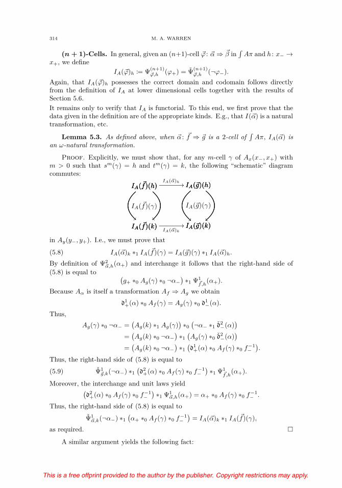
Lemma 5.3. As defined above, when α : f ⇒ g is a 2-cell of∫Aπ, IA(α) is

an ω-natural transformation.

Proof. Explicitly, we must show that, for any m-cell γ of Ax(x−, x+) withm > 0 such that sm(γ) = h and tm(γ) = k, the following “schematic” diagramcommutes:

IA(f)(h) IA(g)(h)IA(�α)h

��IA(f)(h)

IA(f)(k)##

IA(f)(h)

IA(f)(k)��

IA(f)(k) IA(g)(k)IA(�α)k

��

IA(g)(h)

IA(g)(k)��

IA(g)(h)

IA(g)(k)

IA(f)(γ) IA(g)(γ)

in Ay(y−, y+). I.e., we must prove that

(5.8) IA(α)k ∗1 IA(f)(γ) = IA(g)(γ) ∗1 IA(α)h.By definition of Ψ2

�α,h(α+) and interchange it follows that the right-hand side of(5.8) is equal to (

g+ ∗0 Ag(γ) ∗0 ¬α−)∗1 Ψ1

�f,h(α+).

Because Aα is itself a transformation Af ⇒ Ag we obtain

d1+(α) ∗0 Af (γ) = Ag(γ) ∗0 d

1−(α).

Thus,Ag(γ) ∗0 ¬α− =

(Ag(k) ∗1 Ag(γ)

)∗0

(¬α− ∗1 d

2−(α)

)

=(Ag(k) ∗0 ¬α−

)∗1

(Ag(γ) ∗0 d

2−(α)

)

=(Ag(k) ∗0 ¬α−

)∗1

(d1+(α) ∗0 Af (γ) ∗0 f

−1−

).

Thus, the right-hand side of (5.8) is equal to

(5.9) Ψ1�g,k(¬α−) ∗1

(d2+(α) ∗0 Af (γ) ∗0 f

−1−

)∗1 Ψ1

�f,h(α+).

Moreover, the interchange and unit laws yield(d2+(α) ∗0 Af (γ) ∗0 f

−1−

)∗1 Ψ1

�α,h(α+) = α+ ∗0 Af (γ) ∗0 f−1− .

Thus, the right-hand side of (5.8) is equal to

Ψ1�α,k(¬α−) ∗1

(α+ ∗0 Af (γ) ∗0 f

−1−

)= IA(α)k ∗1 IA(f)(γ),

as required. �

A similar argument yields the following fact:



Lemma 5.4. Given parallel n-cells α and β in∫Aπ bounded by 1-cells f,g : x

⇒ y together with a (n+1)-cell ϕ : α ⇒ β, IA(ϕ), as defined above, is a modificationIA(α) ⇒ IA(β).

Proposition 5.5. As defined, IA is a functor∫

(A ◦ π) → ω-Gpd.

Proof. First we consider the case of vertical composition. Let p-cells ϕ andψ be given, for p ≥ m ≥ n + 1 > 1, which are bounded by 0-cells x and y and byn-cells f , g and h as indicated in the following diagram:

u v

�f

��

u v

�h

��u �g�g v��

ϕ

ψ

�α��

�β��

�γ��

�δ��

Then, for any object k : x− → x+ of Ax(x−, x+), we will prove by induction on mthe stronger fact that when m is odd

Ψmsp−m(�ψ∗n�ϕ),k

((ψ ∗n ϕ)+

)= Ψm

s(p−m) �ψ,k(ψ+) ∗n Ψm

s(p−m)�ϕ,k(ϕ+),

Ψmtp−m(�ψ∗n�ϕ),k

(¬(ψ ∗n ϕ)−

)= Ψm

t(p−m) �ψ,k(¬ψ−) ∗n Ψm

t(p−m)�ϕ,k(¬ϕ−);

andΨm

tp−m(�ψ∗n�ϕ),k

((ψ ∗n ϕ)+

)= Ψm

t(p−m) �ψ,k(ψ+) ∗n Ψm

t(p−m) �ϕ,k(ϕ+),

Ψmsp−m(�ψ∗n�ϕ),k

(¬(ψ ∗n ϕ)−

)= Ψm

s(p−m) �ψ,k(¬ψ−) ∗n Ψm

s(p−m)�ϕ,k(¬ϕ−);

when m is even.First, assume m = n+ 1 is even. We also assume that n+ 1 > 2 since the case

where n + 1 = 2 is a straightforward calculation (using ideas essentially the sameas those used here). Then

Ψn+1�δ∗n

�β

((ψ ∗n ϕ)+

)= Ψn

�h

(¬(δ ∗n β)−

)∗n Ψn

�f

((ψ ∗n ϕ)+

)

And this is equal, by definition of composition, to(5.10) Ψn

�h

(¬δ− ∗n (dn−(δ) ∗(n−1) ¬β−)

)∗n Ψn

�f

((ψ+ ∗(n−1) d

n+(β)) ∗n ϕ+

)

Now we will investigate in more detail each of the larger terms in this composite.First:

Ψn�h

(¬δ− ∗n (dn−(δ) ∗(n−1) ¬β−)

)= Ψn

�h(¬δ−) ∗n Ψn

�h

(dn−(δ) ∗(n−1) ¬β−)

).

By definition of Ψn and functoriality this is equal toΨn

�h(¬δ−) ∗n

(Ψn−1

�v (h+) ∗(n−1) Ψn−1�u (dn−(δ)) ∗(n−1) Ψn−1

�u (¬β−)),

which by (5.7) is equal to:

Ψn�h(¬δ−) ∗n

(Ψn−1

�v (h+) ∗(n−1) Ψn−1�v (dn+(δ)) ∗(n−1) Ψn−1

�u (¬β−))

= Ψn�h(¬δ−) ∗n

(Ψn−1

�v (dn+1+ (δ)) ∗(n−1) Ψn−1

�u (¬β−))


316 M. A. WARREN

Similarly, the other half of (5.10) is equal to(Ψn−1

�v (ψ+) ∗(n−1) Ψn−1�u (dn+1

− (β)))∗n Ψn

�f(ϕ+).

By these observations and a routine calculation it follows that (5.10) is equal to

Ψn�h(¬δ−) ∗n

(Ψn−1

�v (ψ+) ∗(n−1) Ψn−1�u (¬β−)

)∗n Ψn

�f(ϕ+).

Finally, using the unit and interchange laws this is seen to be the same as Ψn+1�δ

(ψ+)∗n Ψn+1

�β(ϕ+). The base cases where n + 1 is odd are dual and the induction steps

are trivial. Thus, IA is a functor. �

6. Reflexivity and elimination terms

In this section we define the functors which will interpret reflexivity and elim-ination terms. As in [9] we will interpret terms as sections of the projection map∫A → C associated to the functor A which interprets their type. We begin by

summarizing some of the basic facts about such sections and the related structuresresulting from the Grothendieck construction.

6.1. Reflexivity terms. We end this section by describing briefly the “reflex-ivity term” associated to a functor A : C → ω-Gpd. By definition, the reflexivityterm should be a section rA:

(6.1)

∫A

∫A

1∫A ��

��

��

∫A

∫(IA ◦ δA)rA ��

∫(IA ◦ δA)

∫A��

where δA is as in Section 5.2. However, we will require the explicit description ofthis map and we will also introduce some notation related to this map. For objects,given an object x of

∫A, we must provide an object xr of IA(x, x−, x−). I.e., xr

should be an arrow x− → x− in Ax. We define xr to be the identity x−. (Notethat here and throughout we omit the identity maps and write x− instead of i(x−).)Next, given an arrow f : x → y, we need to provide an arrow

(∂I)1r(�x),r(�y)(f)�fr−→ yr = y−

in Ay, where (∂I)n denotes the weighted face functor for∫IA (and so, in this case,

also∫IAδA). But, by definition, (∂I)1(f) is just y− and we therefore define fr to be

y−. Indeed, at every dimension n ≥ 1, when ϕ is a n-cell of∫A bounded by objects

x and y, we define ϕr to be y−. Alternatively, the map rA may be constructed, asthe anonymous referee was kind enough to mention to us, as the canonical sectioninduced by the fact that

∫(IA ◦ δA)

∫IA��

∫(IA ◦ δA)

∫A��∫A

∫(A ◦ π)

δA

��

∫IA

∫(A ◦ π)

��

is a pullback. Note that r is constant y− in all dimensions n ≥ 1 since (∂I)1r(�x),r(�y)(ϕ)is equal to y− for any ϕ in

∫A bounded by x and y. As such, we define ϕr to be



y− in all dimensions n ≥ 1. With this definition functoriality of r is trivial and wehave proved:

Lemma 6.1. Given A : C → ω-Gpd as above, the assignment r defined aboveinduces a section rA as indicated in (6.1).

6.2. Setting up the construction of elimination terms. Turning now toelimination terms, suppose we are given a functor D :

∫IA → ω-Gpd together

with a section d :∫A →

∫D{δA}IArA of the projection

∫D{δA}IArA →

∫A. We

would like to prove that this extends to a section J of∫D →

∫IA. We begin by

fixing notation.As we are dealing with multiple cases of the Grothendieck construction it will

be convenient to introduce some notation to deal with the different weighted facefunctions which occur. First, we denote by Θn(–) the weighted face functor for∫D. As usual, we denote by dn− and dn+ the functors for the two projections of

∫IA. Finally, we denote by Θn the weighted face functor for

∫D ◦ {δA}IA ◦ rA.

Next, we observe that there is an endofunctor ↓(–) :∫IA →

∫IA defined as

the following composite:∫

IAπ0−−→

∫A

rA−−→∫

IA ◦ δA →∫

IA.

I.e., ↓ sends an object x = (x, x−, x+, x→) to (x, x−, x−, x−) and similarly forhigher-dimensional cells. Here, as throughout, we omit mention of identity arrows.I.e., writing out identities we have that ↓ x is (x, x−, x−, i(x−)) or (x, x−, x−, 1x−).

We will often be concerned with the situation where we consider, given x anobject of

∫IA, the restriction (x, x−) of x to

∫A. Rather than write π0(x) every

time for this object we instead denote this pair by x. Similarly, γ denotes π0(γ) forgeneral n-cells γ of

∫IA.

6.3. Naturality cells. The construction of the elimination terms is rathertechnical and proceeds in several stages. First, we describe “naturality cells” whichexhibit what amounts to a (suitable notion of) pseudo natural transformation ε−from ↓(–) to the identity 1∫

IA. The construction proceeds by induction on dimen-

sion as usual.Dimension 0. First, in dimension 0, given x in

∫IA, we define an arrow

ε�x : ↓(x) → x as follows:ε�x := (x, x−, x→, x→),

where x = (x, x−, x+, x→). Next, holding 0-cells x and y of∫IA fixed we define

functors(∫

IA

)

1(x, y)

∇1�x,�y;ξ−−−−→

(∫IA

)

1(↓ x, y)

for ξ = −,+ as follows:

∇1�x,�y;ξ :=

{(– ∗0 ε�x) if ξ = −,(ε�y∗0 ↓ (–)

)if ξ = +.

As usual, we omit the subscripts x and y when these are understood.


318 M. A. WARREN

Note that with these definitions, when ϕ is any m-cell, with m ≥ 1,∇1

−(ϕ) = (ϕ,ϕ−, ϕ+ ∗0 Af (x→), ϕ→),(6.2)∇1

+(ϕ) = (ϕ,ϕ−, y→ ∗0 ϕ−, y→),(6.3)

where sm−1ϕ = f and f : x → y is as above.

Remark 6.2. Because we will sometimes want to refer to the different elementsof such a pair ∇1

ξ(ϕ) we denote by [∇1ξ(ϕ)]k the kth component, for k = 0, 1, 2, 3.

E.g., [∇1+(ϕ)]2 is (y→ ∗0 ϕ−),.

Dimension 1. Next, we define, given an arrow f : x → y in∫IA, a 2-cell

∇1−(f)

ε�f−→ ∇1+(f).

I.e., ε�f is as indicated in the following “naturality” diagram:

↓(y) yε�y��

↓(x)

↓(y)

↓(�f)��

↓(x) xε�x �� x

y

�f

��ε�f ��

In particular, ε�f is defined to be (f, f−, f→ ∗0 f−, f→). This definition is easily seento make sense using (6.2) and (6.3). Now, holding parallel arrows f and g fixed,we define functors

(∫IA

)

2(f,g)

∇2ξ−−→

(∫IA

)

2

(∇1

−(f),∇1+(g)

)

by

∇2ξ(γ) :=

{∇1

+(γ) ∗1 ε�f if ξ = −,ε�g ∗1 ∇1

−(γ) if ξ = +.With these definitions it is straightforward to verify that(6.4) ∇2

−(ϕ) = (ϕ,ϕ−, f→ ∗0 ϕ−, f→),

when ϕ is any cell of (∫IA)2(f,g). In order to obtain a similar analysis of ∇2

+(ϕ)we require a further fact about the duality functor ¬.

Lemma 6.3. Given any m-cell, for m ≥ 1, ϕ of∫A,

¬ϕ− ∗0 ϕ− = d1�x,�y(ϕ),

ϕ− ∗0 ¬ϕ− = y−

where x and y are the 0-cells bounding ϕ.

Proof. This is a direct consequence of the easily proved fact that, for 0 ≤ n ≤m− 2

ρm−n−2∂�ϕ (ϕ−1

− ) ∗n ϕ− = tm−n−1(ϕ)−− ∗n(ϕ− ∗(n+1) ρ

m−n−3∂�ϕ (ϕ−1

− ))

when n is even (or 0), andϕ− ∗n ρm−n−2

∂�ϕ (ϕ−1− ) =

(ρm−n−3∂�ϕ (ϕ−1

− ) ∗(n+1) ϕ−)∗n sm−n−1(ϕ)−1

− ,

when n is odd. Iteratively applying these facts and canceling inverses yields therequired result. �



Using Lemma 6.3 it follows, by a (lengthy but) straightforward calculation,that, where β

(6.5) ∇2+(ϕ) =

(

ϕ,ϕ−,(g→ ∗1 Ψ2

�β,x→(ϕ+)

)∗0 β−, ϕ→

)

for any m-cell ϕ of (∫IA)2(f,g) with β = tm−2ϕ. Using (6.4) and (6.5) we define

ε�α, for α : f ⇒ g a 2-cell of∫IA, as follows:

ε�α := (α, α−, α→ ∗0 α−, α→).

In higher dimensions this procedure is carried out as follows:Dimension (n + 1). Given α and β of dimension n together with the appro-

priate ∇n− we first observe that, using decompositions of ∇n

ξ (ϕ) corresponding to(6.4) and (6.5), and proved by a standard calculation using Lemma 6.3, it followsthat, if, ϕ : α ⇒ β is a (n + 1)-cell, then

∇n−(ϕ) =

{(ϕ,ϕ−, α→ ∗0 ϕ−, α→) if n is even,(ϕ,ϕ−, (∂I)n(ϕ) ∗0 ϕ−, ϕ→) if n is odd;

and

∇n+(ϕ) =

{(ϕ,ϕ−, (∂I)n(ϕ) ∗0 ϕ−, α→) if n is even,(ϕ,ϕ−, β→ ∗0 ϕ−, β→) if n is odd.

Thus we define∇n

−(α)ε�ϕ−→ ∇n

+(β)by

(ϕ,ϕ−, ϕ→ ∗0 ϕ−, ϕ→).

Now, holding α and β fixed, we define(∫

IA

)

n+1(α, β)

∇n+1ξ−−−→

(∫IA

)

n+1

(∇n

−(α),∇n+(β)

)

for ξ = −,+ as

∇n+1ξ (γ) :=

{∇n

+(γ) ∗n ε�α if ξ = −,ε�β ∗n ∇n

−(γ) if ξ = +.

6.4. Elimination terms in dimensions 0, 1. Assume we are given an objectx = (x, x−, x+, x→) of

∫IA. We would like to provide a corresponding object, which

for the sake of notational convenience we simply denote by xJ , of D(x). This xJ

is obtained by a kind of Yoneda style argument. Namely, we observe that, byassumption there is a term xd in D(↓(x)). Applying the functor D(ε�x) yields therequired xJ in D(x). I.e.,

xJ := D(ε�x)(xd).Because it will greatly simplify matters in the later stages, we introduce a specialnotation for D(ε�x) and its higher-dimensional generalizations D(ε�γ). Namely, wedefine

〈γ〉 := D(ε�γ).With this notation xJ = 〈x〉(xd).


320 M. A. WARREN

In dimension 1, given an arrow f : x → y in∫IA we have by hypothesis the

arrow fd : Θ1x,y(f) → yd in D(↓ y) and, applying 〈y〉,

〈y〉(Θ1f

) 〈�y〉(fd)−−−−→ yJ

in D(y). Now,〈y〉

(Θ1f

)= 〈y〉

(D(↓ f)xd

)= D

(∇1

+f)xd.

Also,Θ1(f) = D(f)(xJ) = D

(∇1

−f)xd

and therefore we define fJ to be the composite

Θ1(f)〈�f〉xd−−−→ D

(∇1

+f)xd

〈�y〉fd−−−→ yJ .

Again, it will be useful to introduce some additional notation to clarify the situationin higher-dimensions. First, holding fixed objects x and y of

∫IA, we define a

functor (∫IA

)

1(x, y)

ϑ1�x,�y−−−→ D(y)

byϑ1�x,�y(γ) := 〈y〉

(Θ1

�x,�y(γ)).

The next ingredient is to define, for f : x → y, arrows �(f) : Θ1(f) → ϑ1(f) and�(f) : ϑ1(f) → yJ as follows:

�(f) := 〈f〉xd,

�(f) := 〈y〉fd.

Thus, with this notation fJ is just �(f) ∗0 �(f). We will see below that, in general,γJ will always be formed as a composite of the form �(γ)∗k−1�(γ) along a (k−1)-cellϑk(γ).

6.5. Elimination terms in dimensions 2. In dimension 2, let arrows f,g : x⇒ y in

∫IA be given together with a 2-cell α : f ⇒ g. In order to define αJ we

will describe 2-cells filling both the square and triangle as indicated in the followingdiagram:

Θ1(f) ϑ1(f)�(�f)

��Θ1(f)

Θ1(g)

Θ1(�α)

��

ϑ1(f) yJ�(�f)

��

Θ1(g) ϑ1(g)�(�g)

��

ϑ1(f)

ϑ1(g)

ϑ1(�α)

��

ϑ1(g)

yJ

�(�g)

��

��

Defining the functor(∫

IA

)

2(f,g)

ϑ2�f,�g−−−→ D(y)1

(Θ1(f), yJ

)

byϑ2(–) := �(g) ∗0 ϑ

1(–) ∗0 �(f).



we see that our goal is precisely to provide 2-cells

fJ�(�α)−−−→ ϑ2

�f,�g(α) �(�α)−−−→ Θ2

�f,�g(α).

The strategy for filling the square and triangle from above is fairly simple. For thetriangle, we use αd, and for the square we use the naturality cell ε�α. To begin with,we define

�(α) := 〈y〉(αd) ∗0 �(f).For the square, we observe that

Θ1(γ) = D(γ)(xJ),ϑ1(γ) = D(∇1

+γ)(xd)

where γ is any cell of∫IA(x, y). Thus,

ϑ1(γ) ∗0 �(f) = D(∇2−γ)(xd),

�(g) ∗0 Θ1(γ) = D(∇2+γ)(xd).

As such, we define�(α) := �(g) ∗0 〈α〉xd

.

Thus, αJ is (�(α) ∗1 �(α)). It will often be convenient to omit parentheses whendealing with the arrows �(α) and �(α). In order to avoid confusion, we adopt theconvention that � and � bind more tightly than composition. I.e., �γ ∗k ϕ shouldbe read as �(γ) ∗k ϕ.

Before moving on to dimension 3, we first introduce some additional machinerywhich is the final technical ingredient required in order to make the induction tohigher dimensions possible. Namely, for f,g : x ⇒ y parallel 1-cells, we definefunctors

D(y)1(ϑ1 f, yJ )H1

�f,�g−−−→ D(y)1(Θ1 f, yJ )H1

�f,�g−−−→ D(y)1(Θ1 f, ϑ1g)

as follows:

H1�f,�g

(–) := (– ∗0 � f),

H1�f,�g

(–) := (�g ∗0 –).

With these functors at our disposal, we are in the position to make several remarksregarding their interaction with the other structures with which we are concerned.To begin with, when α is a 2-cell f ⇒ g,

� α = H1�f,�g

(〈α〉xd

),(6.6)

� α = H1�f,�g

(〈y〉(αd)

).(6.7)

Also, these functors interact with ϑ2 in the sense that

H1�f,�g

(�g ∗0 ϑ

1(γ))

= ϑ2�f,�g

(γ) = H1�f,�g

(ϑ1(γ) ∗0 � f

).(6.8)

In an informal sense, the problem of providing the elimination maps ϕJ will be seento always amount, as above, to filling both a triangle and a square. In each case,the tactic is essentially the same as above and the functors Hk and Hk allow usto express in the most perspicuous way the combinatorics of the situation for thesquares and triangles, respectively.


322 M. A. WARREN

6.6. Elimination terms in dimension 3. In dimension 3, given ϕ : α ⇒ βa 3-cell of

∫IA, we would like to describe the 3-cells indicated in the following

diagram:

(6.9)

ϑ2(α) Θ2(α)� �α ��ϑ2(α)

ϑ2(β)

ϑ2(�ϕ)

��

fJ ϑ2(α)� �α ��

ϑ2(β) Θ2(β)� �β

��

Θ2(α)

Θ2(β)

Θ2(�ϕ)

��

fJ

ϑ2(β)� �β

$$

��

With this picture in mind we begin by defining, for fixed parallel 2-cells α, β : f ⇒ g,functors

D(y)2(fJ , ϑ2β)H2

�α,�β−−−→ D(y)2(fJ ,Θ2β)H2

�α,�β−−−→ D(y)2(ϑ2α,Θ2β)

as follows:

H2�α,�β

(–) := � β ∗1 H1�f,�g

(–),

H2�α,�β

(–) := H1�f,�g

(–) ∗1 � α.

Next,(∫

IA

)

3(α, β)

ϑ3�α,�β−−−→ D(y)2

(fJ ,Θ2(β)

)

is defined byϑ3(–) := �(β) ∗1 ϑ

2(–) ∗1 �(α)Before going any further it is useful to establish several facts. First, we note thatby a straightforward calculation:

(6.10) ϑ2�f,�g

(γ) = H1�f,�g

(〈y〉Θ2γ

).

We call (6.10) the triangle-law for dimension 2 and note that together with (6.7)it follows that the triangle from (6.9) may be filled with the 3-cell H1

�f,�g(〈y〉ϕd).

Accordingly, we define� ϕ := H2

�α,�β

(〈y〉ϕd

).

Turning to the square, observe that

Θ2�f,�g

(γ) ∗1 � α = (gJ ∗0 Θ1γ) ∗1 (�g ∗0 〈α〉xd)

= (�g ∗0 �g ∗0 Θ1γ) ∗1 (�g ∗0 〈α〉xd)

= �g ∗0((�g ∗0 Θ1γ) ∗1 〈α〉xd

)

= �g ∗0 D(∇3

−γ)xd.

Consequently, we obtain the source square-law for dimension 2 :

(6.11) Θ2�f,�g

(γ) ∗1 � α = H1�f,�g

(D(∇3

−γ)xd

).

Another straightforward calculation yields the target square-law for dimension 2:

(6.12) � β ∗1 ϑ2�f,�g

(γ) = H1�f,�g

(D(∇3

+γ)xd

).



Thus, the filler of the square in (6.9) is defined to be H1�f,�g

(〈ϕ〉xd

). Finally, we set

� ϕ := H2�α,�β

(〈ϕ〉xd

),

ϕJ := � ϕ ∗2 � ϕ.

6.7. The construction in higher dimensions. Now, at higher dimensions,the construction of the elimination terms is by induction on dimension. In partic-ular, we proceed by induction on n ≥ 2 in such a way that at stage (n + 1)— inaddition to the existence of the required (n+1)-cells ϕJ —the following conditionsare satisfied:

(1) For all parallel n-cells α, β : f ⇒ g, there is a functor ϑn+1�α,�β

parallel to Θn+1�α,�β

.I.e., .

(2) For any (n + 1)-cell ϕ : α → β, there exist corresponding (n + 1)-cells � ϕand � ϕ such that

αJ� �ϕ−−→ ϑn+1

�α,�βϕ

� �ϕ−−→ Θn+1�α,�β

ϕ

when (n + 1) is even, and

Θn+1�α,�β

ϕ� �ϕ−−→ ϑn+1

�α,�βϕ

� �ϕ−−→ βJ

when (n + 1) is odd.(3) There are, for α and β parallel n-cells, functors Hn

�α,�βand Hn

�α,�βsuch that

D(y)n(ϑnα, gJ

) Hn

�α,�β−−−→ D(y)n(Θnα, gJ

),

D(y)n(Θnα, ϑnβ

) Hn

�α,�β−−−→ D(y)n(Θnα, gJ

)

if (n + 1) is even; and

D(y)n(fJ , ϑ

nβ) Hn

�α,�β−−−→ D(y)n(fJ ,Θnβ

),

D(y)n(ϑnα,Θnβ

) Hn

�α,�β−−−→ D(y)n(fJ ,Θnβ

)

if (n + 1) is odd.(4) The following triangle-law is satisfied:

ϑn+1�α,�β

γ = Hn�α,�β

(〈y〉Θn+1γ

),

when γ is any cell in the domain of ϑn+1.(5) If ϕ, ψ : α ⇒ β are parallel (n + 1)-cells, the following square-laws are

satisfied:

Hn�α,�β

(D(∇n+2

− γ)xd

)=

{Θn+1γ ∗n � ϕ if (n + 1) is even,ϑn+1γ ∗n � ϕ if (n + 1) is odd;

and

Hn�α,�β

(D(∇n+2

+δ)xd

)=

{� ψ ∗n ϑn+1δ if (n + 1) is even,� ψ ∗n Θn+1δ if (n + 1) is odd,

for appropriate cells γ and δ. Note that the ∇n+2ξ here are defined with respect to

ϕ and ψ.


324 M. A. WARREN

Assuming we have carried out the construction up to stage n, we claim thatthe following definitions at stage (n + 1) will satisfy the required conditions:

• For parallel n-cells α and β,

ϑn+1�α,�β

(–) := � α ∗(n−1) ϑn(–) ∗(n−1) � β.

• If α and β are parallel n-cells f ⇒ g, then we define

Hn�α,�β

(–) :=

{�β ∗n Hn−1

�f,�g(–) if (n + 1) is even,

Hn−1�f,�g

(–) ∗n � α if (n + 1)is odd;

and

Hn�α,�β

(–) :=

{Hn−1

�f,�g(–) ∗n � α if (n + 1) is even,

� β ∗n Hn−1�f,�g

(–) if (n + 1) is odd.

• Given ϕ : α ⇒ β a (n + 1)-cell, we define

� ϕ :=

{Hn

�α,�β

(〈y〉ϕd

)if (n + 1) is even,

Hn�α,�β

(〈ϕ〉xd

)if (n + 1) is odd;

and

� ϕ :=

{Hn

�α,�β

(〈ϕ〉xd

)if (n + 1) is even,

Hn�α,�β

(〈y〉ϕd

)if (n + 1) is odd.

• In all dimensions,αJ := � α ∗n � α

when α is a (n + 1)-cell.The reader can readily verify that we have already satisfied the conditions of

the induction in the base case where n = 2. We now turn to the induction step.

Lemma 6.4. With the definitions given above, the conditions of the construc-tion are satisfied in all dimensions (n + 1).

Proof. First, assume (n + 1) is even with n > 2 and let an (n + 1)-cellϕ : α ⇒ β in

∫IA be given. Then, by the induction hypothesis and examination of

the following diagram

Θn(α) ϑn(α)� �α ��Θn(α)

Θn(β)

Θn(�ϕ)

��

ϑn(α) gJ� �α ��

Θn(β) ϑn(β)� �β

��

ϑn(α)

ϑn(β)

ϑn(�ϕ)

��

ϑn(β)

gJ

� �β

��

��

where α, β : f ⇒ g, it follows that conditions (1) – (3) are satisfied with the defini-tions given above.



For the triangle law, we reason as follows:

Hn�α,�β

(〈y〉Θn+1γ

)= Hn−1

�f,�g

(〈y〉βd ∗(n−1) 〈y〉Θnγ

)∗(n−1) � α

= Hn−1�f,�g

(〈y〉βd

)∗(n−1) H

n−1�f,�g

(〈y〉Θnγ

)∗(n−1) � α

= � β ∗(n−1) ϑn�f,�g

(γ) ∗(n−1) � α

= ϑn+1�α,�β

(γ),

where the penultimate equation is by definition of � β and the induction hypothesis.Next assume given (n + 1)-cells ϕ, ψ : α ⇒ β. For the “source” square law, we

have

Hn�α,�β

(D(∇n+2

− γ)xd

)= Hn

�α,�β

(D(∇n+1

+ γ)xd∗n 〈ϕ〉xd

)

=(

� β ∗(n−1) Hn−1�f,�g

(D(∇n+1

+ γ)))

∗n � ϕ

=(� β ∗(n−1) � β ∗(n−1) Θnγ

)∗n � ϕ

=(βJ ∗(n−1) Θnγ

)∗n � ϕ

= Θn+1�α,�β

γ ∗n � ϕ,

where the third equation is by the induction hypothesis. For the “target” squarelaw, we reason similarly and note that

Hn�α,�β

(〈ψ〉xd

∗n D(∇n+1− γ)xd

)= � ψ ∗n

(� β ∗(n−1) H

n−1�f,�g

(D(∇n+1

− γ)xd

))

= � ψ ∗n(� β ∗(n−1) ϑ

nγ ∗(n−1) � α)

= � ψ ∗n ϑn+1�α,�β

γ,

as required.The induction step where (n + 1) is odd is essentially dual. �

Using the lemma, we now have the following fundamental result.

Proposition 6.5. The cells of the form ϕJ constitute a section J :∫IA →

∫D

of the projection map∫D →

∫IA.

Proof. In light of Lemma 6.4 the only thing which remains is to verify thatthe assignment (–)J is functorial. This however is a consequence of the functorialityof d and the construction of the “terms” ϕJ using the functors Hk and Hk. �

7. The main results

With the machinery from the preceding sections at our disposal it is now pos-sible to establish our main results.

7.1. Dependent sums and products. Before defining the dependent prod-ucts and sums, we begin by describing some basic features of general setup. First,given a functor A : C → ω-Gpd we note that, by the basic properties of ω-Gpd,there exists an ω-groupoid denoted by Γ(A) of sections of the projection

∫A → C.


326 M. A. WARREN

I.e., the objects of Γ(A) are sections

C

C1C

��

��

��C

∫A

a ��∫A

Cπ

��

and arrows are 2-cells α : a ⇒ b for which π ◦ α = 1C and so forth at higherdimensions. Now, given a further functor B :

∫A → ω-Gpd and an object x of C,

we define a functor �Bx� : Ax → ω-Gpd as follows:Objects. Given an object x− of Ax, �Bx�(x−) is the ω-groupoid B(x, x−).1-Cells. Given an arrow h : x− → x+ in Ax, we define the functor �Bx�(h):

B(x, x−) → B(x, x+) as follows:

�Bx�(h)(–) := B(x, h)(–).

Here we note that this is possible since (x, h) : (x, x−) → (x, x+), where we havewritten (x, h) instead of (1x, h).

(n + 1)-Cells Given a (n+1)-cell α : f ⇒ g in Ax bounded by 0-cells x− andx+, together with an object y of B(x, x−), the transformation �Bx�(α) is definedat y by

�Bx�(α)y := B(x, α)y.Now, we would like to describe, in this same setting, the dependent sum ΣA,B : C →ω-Gpd. Note that, when A and B are apparent, we will often omit the subscripts.

Objects. Given an object x of C, we define

ΣA,B(x) :=∫

�Bx�.

Given f : x → y in C we would like to define ΣA,B(f) :∫�Bx� →

∫�By�, which

we will write, for the sake of avoiding too many parentheses, as Σf . An object vof

∫�Bx� is a pair (v−, v�) such that v− is an object of Ax and v� is an object of

B(x, v−). We adopt a similar notation in higher dimensions. We also write ∂(x)nfor the weighted face functor of

∫�Bx� and similarly for ∂(y)n, etc. With this in

mind we adopt the following definition (which we will discuss below):1-Cells. Given f : x → y in C, Σf is defined on objects v of

∫�Bx� by

Σf (v) :=(v−.f, B(f, v−.f)(v�)

),

and on (n + 1)-cells ϕ of∫�Bx� by

Σf (ϕ) :=(ϕ−.f, B(f, w−.f)(ϕ�)

),

where v and w are the objects bounding ϕ at source and target position, respec-tively.Note that this is a correct definition since, by functoriality of B, it is proved (si-multaneously with the verification of the definitions) at each stage that

B(f, w−.f)(∂(x)n+1

�α,�β(ϕ−)

)= ∂(y)n+1

Σf �α,Σf�β(ϕ−.f),

where α and β are the n-cells bounding ϕ.In dimension (n + 1), ΣA,B is given as follows:



(n + 1)-Cells. Given a (n + 1)-cell ϕ : α → β in C, Σϕ : Σα → Σβ has as itscomponent at the object v of

∫�Bx� the n-cell

(Σϕ)�v :=(v−.ϕ,B(ϕ, v−.ϕ)(v�)

)

of∫�By�.

To see that this makes sense, let n-cells λ, μ : α → β be given. Then it follows, byinduction on n that,

∂(y)(n+1)(Σλ)�v,(Σμ)�v(v−.γ) =

{B(μ, v−.γ)v if (n + 1) is even,B(λ, v−.γ)v if (n + 1) is odd,

where γ is any m-cell with m ≥ n + 1 bounded by λ and μ (i.e., sm−nγ = λand tm−nγ = μ). This is a straightforward induction using functoriality of B.This completes the description of the interpretation ΣA,B of dependent sums inthis setting. With these definitions, the verification of functoriality is a routinecalculation.

Next, we define the dependent product ΠA,B : C → ω-Gpd to be the functorwhich sends an object x to the ω-groupoid Γ(�Bx�) of sections of the projection∫�Bx� → Ax. Explicitly, ΠA,B is as follows:

Objects. ΠA,B(x) is defined to be Γ(�Bx�).1-Cells. Given an arrow f : x → y in C, ΠA,B(f) is the functor sending a

section a in Γ(�Bx�) to the section Σf ◦ a ◦ Af−1 . In general, ΠA,B(f) sends anarbitrary cell ϕ of Γ(�Bx�) to the composite Σf ◦ ϕ ◦ Af−1 as indicated in thefollowing diagram:

Ay Ax

Af−1�� Ax

∫�Bx�

%%

Ax

∫�Bx�

&&

∫�Bx�

∫�By�

Σf��∫�By�

Ay

��

∫�Bx�

Ax

��

Ax AyAf

��

ϕAx

Ax

1Ax

(n + 1)-Cells. In general, when γ : α → β is a (n + 1)-cell in C and a is anobject of ΠA,B(x), the dependent product is defined by setting

ΠA,B(γ)a := Σγ ◦ a ◦Aσ(γ),

where σ : C → Cop is the dual functor for C as described in Section 4.This completes the description of the dependent sums and products. The introduc-tion and elimination terms are then obtained as generalizations of those given in[9].

7.2. Results. With the interpretations given we obtain the following resultextending the original groupoids model from ibid. to the setting of ω-groupoids:

Theorem 7.1. The interpretation given above soundly interprets the basicform of intensional type theory with dependent sums, dependent products and iden-tity types (i.e., the theory Tω from [1]). Moreover, the η-rules for dependent sumsand products are also satisfied.

Proof. Using the interpretation given above it is straightforward to verify thatall of the required laws, including all of the Beck – Chevalley laws, are satisfied. �


328 M. A. WARREN

Recall from [1, 27] that we employ the following notation for iterated identitytypes:

An+1(a1, b1; . . . ; an+1, bn+1) := An(a1, b1; . . . ; an, bn)(an+1, bn+1).

In this notation, the principle of n-dimensional uniqueness of identity proofs is

� an+1, bn+1 : An(a1, b1; . . . ; an, bn)� an+1 = bn+1 : An(a1, b1; . . . ; an, bn)

It is a trivial consequence of the interpretation that, for all n ≥ 1, the ω-groupoidmodel refutes UIPn. To see this, form the globular set G which is described asfollows:

0-Cells. Two 0-cells ⊥0 and �0.(n + 1)-Cells. Two parallel (n + 1)-cells ⊥n+1,�n+1 : ⊥n→ �n.

Then the free ω-groupoid on G refutes uniqueness of identity proofs at all dimen-sions (in both the forms which deal with definitional and propositional equality).This is the case because the terms of identity types in any type interpreted as thisfree groupoid are simply the cells of this groupoid. I.e., we have:

Corollary 7.2. For all n ≥ 1, the principle UIPn is not derivable in Tω.Similar, the principle of uniqueness of identity proofs with respect to propositionalequality is also not derivable.

Recall from [1] that the n-truncation rule is as follows:

� an+1, bn+1 : An(a1, b1; . . . ; an, bn) � p : An+1(a1, b1; . . . ; an+1, bn+1) TRn� an+1 = bn+1 : An(a1, b1; . . . ; an, bn)Our main corollary of Theorem 7.1 then states that the identity types in intensionaltype theory are nontrivial in all dimensions in the sense that all of the truncationrules are refuted by the ω-groupoid model. The same counterexample from abovesuffices to give this result as well. I.e., we have:

Corollary 7.3. For n ≥ 0, TRn is not derivable in Tω.

We note that all of these results also apply in the case of type theory with theadded η-rules for dependent products and sums, since these rules are valid in themodel.

Appendix A. Rules governing identity types,dependent products and dependent sums

In this appendix we describe the syntax of the system considered in this paper(called Tω in [1]). All rules below are stated in an ambient context which is omittedfor ease of presentation.

A.1. Identity types.

a, b : A formation� A(a, b) : type

a : A introductionr(a) : A(a, a)



x : A, y : A, z : A(x, y) � B(x, y, z) : typex : A � ϕ(x) : B

(x, x, r(x)

)

f : A(a, b)elimination

J(ϕ(x), a, b, f) : B(a, b, f)

a : A conversionJ(ϕ(x), a, a, r(a)

)= ϕ(a) : B

(a, a, r(a)

)

A.2. Dependent products.

x : A � B(x) : type ∏formation∏

x:A B(x) : type

x : A � f(x) : B(x) ∏introduction

λx:Af(x) :∏

x:AB(x)

f :∏

x:AB(x) a : A ∏elimination

app(f, a) : B(a).

λx:Af(x) :∏

x:A B(x) a : A ∏conversion

app(λx:Af(x), a

)= f(a) : B(a)

A.3. Dependent sums.

x : A � B(x) : type ∑formation∑

x:A B(x) : type

a : A b : B(a) ∑introduction

pair(a, b) :∑

x:A B(x)

p :∑

x:A B(x) x : A, y : B(x) � ψ(x, y) : C(pair(x, y)

)∑

eliminationR(ψ(x, y), p

): C(p)

a : A b : B(a) x : A, y : B(x) � ψ(x, y) : C(pair(x, y)

)∑

conversionR(ψ(x, y), pair(a, b)

)= ψ(a, b) : C

(pair(a, b)

)

Appendix B. The universal property of the Grothendieck construction

In this appendix we provide a detailed proof that the Grothendieck construction∫A for strict ω-categories introduced in Section 3 can be described as the coend∫ x(x ↓ C) × Ax. First we turn to a more detailed description of the comma ω-

category (x ↓ C) when x is a 0-cell of an ω-category C.


330 M. A. WARREN

B.1. The comma ω-category. Given an ω-category C and an object x ofC the comma ω-category (x ↓ C) will be constructed inductively in such a waythat at each stage a n-cell of (x ↓ C) is a pair (f, f−) such that f is a n-cell of Cand f− is a (n + 1)-cell of C. At each stage it will also be necessary to constructauxiliary functors which describe the boundaries of the cells f− in terms of f andlower dimensional cells. These are like the weighted face functors discussed in theconstruction of the Grothendieck construction given above and we denote themalso using the notation d. Because we will not require the combinatorial details ofthe comma category (x ↓ C) we will merely describe the different cells and leavethe proof that this yields an ω-category to the reader. We mention that slicingconstructions in the higher-dimensional setting have been studied in recent workby Palm [20].

0-Cells. A 0-cell of (x ↓ C) is a pair y = (y, y−) such that y is an object ofC and y− is an arrow x → y in C. For fixed 0-cells y, z define ∂�y,�z(–) := − ∗0 y−.When y, z are understood the subscript will be omitted.

1-Cells. A 1-cell y → z of (x ↓ C) is a tuple f = (f, f−) with f : y → z a 1-cellin C and f− : ∂(f) → z− a 2-cell in C. Fixing parallel 1-cells f,g : y → z, we define∂�f,�g(–) := g− ∗1 ∂(–).

(n + 1)-Cells for (n + 1) even. A (n+1)-cell ϕ : γ → δ is given by a (n+1)-cell ϕ : γ → δ in C and a (n+2)-cell ϕ− : γ− → ∂(ϕ) in C. Given parallel (n+1)-cellsϕ and ψ we define ∂�ϕ,�ψ(–) := ∂(–) ∗n+1 ϕ−.

(n + 1)-Cells for (n + 1) odd. A (n+1)-cell ϕ : γ → δ is given by a (n+1)-cell ϕ : γ → δ in C and a (n+2)-cell ϕ− : ∂(ϕ) → δ− in C. Given parallel (n+1)-cellsϕ and ψ we define ∂�ϕ,�ψ(–) := ψ− ∗n+1 ∂(–).

Here we use the notation ∂ instead of d to describe the required “weighted bound-aries” of the construction since we will be mixing both the Grothendieck construc-tion and its d and comma categories in Section B.2 below.

Allowing x to vary we obtain a functor (of ω-categories) (− ↓ C) : Cop → ω-Catwhich we describe as follows.

Dimension 1. Given an arrow l : v → x in Cop we have a functor l∗ : (x ↓ C) →(v ↓ C) which sends a cell ϕ = (ϕ,ϕ−) of any dimension of (x ↓ C) to

l∗(ϕ) := (ϕ,ϕ− ∗0 l).

This is trivially functorial.Dimension 2. Given parallel arrows l,m : v → x in C and a 2-cell λ : l → m

the induced transformation λ∗ : l∗ → m∗ has as its component at an object y =(y, y−) of (x ↓ C) the cell

(λ∗)�y := (1y, y− ∗0 λ).

With this definition the naturality condition for natural transformations of ω-categories is straightforward.

Dimension n > 2. Given parallel (n − 1)-cells α and β in C (bounded by vand x, respectively, at dimension 0), and a n-cell ϕ : α → β, the component ofthe induced transformation ϕ∗ : α∗ → β∗ at an object y of (x ↓ C) is given by(1y, y− ∗ ϕ). This clearly satisfies the naturality condition.This process is clearly functorial (since it is just given by precomposition).



B.2. Description of the coend inclusions. We now turn to the descriptionof the coend inclusion functors ιx : (x ↓ C)×Ax →

∫A, for A : C → ω-Cat. Again,

ιx is given by an inductive construction where we must verify certain equations ateach stage. We will begin with the first few dimensions and then we will explainprecisely the conditions of the induction.

0-Cells. A 0-cell of (x ↓ C)×Ax is a tuple y = (y, y−, yo) such that y is a 0-cellof C, y− is a 1-cell y− : x → y in C, and yo is an object of Ax. We define

ιx(y) := (y, yo · y−).

So, in particular, ιx(y)− = yo · y−.Now, given two 0-cells y and z of (x ↓ C)×Ax we have the weighted boundary

functors ∂�y,�z(–) (for (x ↓ C)) and dιx(�y),ιx(�z)(–) (for∫A). These two functors are

moreover related by the law

(B.1) dιx(�y),ιx(�z)(–) = yo · ∂�y,�z(–)

sincedιx(�y),ιx(�z)(–) = yo · y− · − = yo · (– ∗0 y−) = yo · ∂�y,�z(–).

1-Cells. A 1-cell f : y → z of (x ↓ C) ×Ax is a tuple f = (f, f−, fo) such thatf is a 1-cell f : y → z in C, f− : ∂�y,�z(f) → z− is a 2-cell in C, and fo : yo → zo is a1-cell in Ax. Then ιx(f) is defined to be the pair (f, ιx(f)−) where ιx(f)− is the1-cell

dιx(�y),ιx(�z)(f) yo · ∂�y,�z(f)yo · ∂�y,�z(f) yo · z−yo·f−

�� yo · z− zo · z−,fo·z−

��

where the equation is by (B.1). I.e.,

ιx(f)− := (fo · z−) ∗0 (yo · f−).

Now, before moving on to the next stage we observe that, for 1-cells f,g of (x ↓C) ×Ax, the following equation relating the weighted boundary functors holds:

(B.2) dιx(�f),ιx(�g)(–) = (go · z−) ∗0 (yo · ∂�f,�g(–)),

since

dιx(�f),ιx(�g)(–) = ιx(g)− ∗0 dιx(�y),ιx(�z)(–)

=((go · z−) ∗0 (yo · g−)

)∗0

(yo · ∂�y,�z(–)

)

= (go · z−) ∗0(yo · (g− ∗1 ∂�y,�z(–))

)

= (go · z−) ∗0 (yo · ∂�f,�g(–)),

where the first equation is by definition of ∂ιx(�f),ιx(�g)(–), the second equation is by(B.1), the third equation is by associativity of ∗0 and functoriality of A, and thefourth equation is by definition of ∂�f,�g(–).

2-Cells. A 2-cell α : f → g in (x ↓ C) × Ax consists of a tuple α = (α, α−, αo)such that α : f → g is a 2-cell in C, α− is a 3-cell α− : f− → ∂�f,�g(α) in C, and αo

is a 2-cell αo : fo → go in Ax. Then ιx(α) is a pair (α, ιx(α)−) where ιx(α)− is the


332 M. A. WARREN

2-cell

ιx(f)−

(fo · z−) ∗0 (yo · f−)(fo · z−) ∗0 (yo · f−) (go · z−) ∗0(yo · ∂�f,�g(α)

).

(αo·z−)∗0(yo·α−)�� (go · z−) ∗0

(yo · ∂�f,�g(α)

).

dιx(�f),ιx(�g)

(α)

I.e.,ιx(α)− := (αo · z−) ∗0 (yo · α−).

Again, for 2-cells α and β of (x ↓ C) ×Ax, there is an equation

(B.3) dιx(�α),ιx(�β)(–) = (αo · z−) ∗0 (yo · ∂�α,�β(–))

relating the weighted boundary functors. This equation is obtained as follows:dιx(�α),ιx(�β)(–) = d

ιx(�f),ιx(�g)(–) ∗1 ιx(α)−

=((go · z−) ∗0 (yo · ∂�f,�g(–)

)∗1

((αo · z−) ∗0 (yo · α−)

)

= (αo · z−) ∗0(yo · (∂�f,�g(–) ∗2 α−)

)

= (αo · z−) ∗0 (yo · ∂�α,�β(–)),

where the penultimate equation is by the interchange law and functoriality of A.3-Cells. A 3-cell ϕ : α → β of (x ↓ C)×Ax is a tuple ϕ = (ϕ,ϕ−, ϕo) such that

ϕ : α → β is a 3-cell in C, ϕ− is a 4-cell ϕ− : ∂�α,�β(ϕ) → β− in C, and ϕo : αo → βo

is a 3-cell in Ax. Then ιx(ϕ) is the pair (ϕ, ιx(ϕ)−) where ιx(ϕ)− is the 3-cell

dιx(�α),ιx(�β)

(ϕ)

(αo · z−) ∗0 (yo · ∂�α,�β(ϕ))(αo · z−) ∗0 (yo · ∂�α,�β(ϕ)) (βo · z−) ∗0 (yo · β−).(ϕo·z−)∗0(yo·ϕ−)

�� (βo · z−) ∗0 (yo · β−).

ιx(β)−

in Az. I.e.,ιx(ϕ)− := (ϕo · z−) ∗0 (yo · ϕ−).

Now, given two 3-cells ϕ, ψ : α → β in (x ↓ C) ×Ax, we have the equation

(B.4) dιx(�ϕ),ιx(�ψ)(–) = (ψo · z−) ∗0 (yo · ∂�ϕ,�ψ(–)),

sincedιx(�ϕ),ιx(�ψ)(–) = ιx(ψ)− ∗2 dιx(�α),ιx(�β)(–)

=((ψo · z−) ∗0 (yo · ψ−)

)∗2

((αo · z−) ∗0 (yo · ∂�α,�β(–))

)

= (ψo · z−) ∗0(yo · (ψ− ∗3 ∂�α,�β(–))

)

= (ψo · z−) ∗0 (yo · ∂�ϕ,�ψ(–))

Indeed, as suggested by these cases, we define at all subsequent stages of the con-struction

(B.5) ιx(ξ)− := (ξo · z−) ∗0 (yo · ξ−),

and that we must verify that the equation

(B.6) dιx(�ξ),ιx(�ζ)(–) = (ζo · z−) ∗0 (yo · ∂�ξ,�ζ(–)



holds. However, the verification that this equation holds generalizes directly fromthe cases of dimensions 2 and 3 given above (since the definitions of d and ∂ alsogeneralize directly from these cases). That ιx is functorial is straightforward and isleft to the reader.

The functors ιx, for x an object of C, constitute a dinatural transformation(− ↓ C) × A− →

∫A in the sense that, for any l,m : v → x in C and any n-cell ϕ

bounded by l and m (including the degenerate case where l = m = ϕ), the diagram

(x ↓ C) ×Av (v ↓ C) × Av

l∗×Av

''

(x ↓ C) ×Av

(x ↓ C) ×Ax

(x↓C)×Al

((

(x ↓ C) ×Av (v ↓ C) × Av

m∗×Av

))(x ↓ C) ×Av

(x ↓ C) ×Ax

(x↓C)×Am

**

(v ↓ C) × Av

∫A

ιv

��

(x ↓ C) ×Ax

∫Aιx

��

ϕ∗×Av

(x↓C)×Aϕ

in ω-Cat commutes. To see this note that, for 0-cells y = (y, y−, yo) of (x ↓ C)×Av,ιv ◦ (l∗ ×Av)(y) = (y, yo · (y− ∗0 l)) = (y, yo · l · y−) = ιx ◦ ((x ↓ C) ×Al)(y),

and, for ϕ any higher dimensional cell bounded by 0-cells y and z, we haveιv ◦ (l∗ ×Av)(ϕ) =

(ϕ, (ϕo · (z− ∗0 l)) ∗0 (yo · (ϕ− ∗0 l))

)

=(ϕ, (ϕo · l · z−) ∗0 (yo · l · ϕ−)

)

= ιx ◦ ((x ↓ C) ×Al)(ϕ).

B.3. Verification of the universal property. We will now show that theι− constitute the universal dinatural transformation of this form. I.e., we prove thatif A is any ω-category together with a family of dinatural transformations (in theω-categorical sense of a ω-categorical natural transformation) ξ : (− ↓ C)×A− → A,then there exists a canonical functor (of ω-categories) F :

∫A → A such that

(x ↓ C) × Ax

∫A

ιx ��(x ↓ C) × Ax

Aξx ��

∫A

A

F

��

(B.7)commutes for every object x of C. The construction of F is a fairly involved induc-tion on dimension. In particular, we will need to construct, for each pair of n-cellsα, β, auxiliary functors ��α,�β(–, –) and ��α,�β(–) (the domains and codomains of thesefunctors will be clear from the description given below). Moreover, we will proveat each stage that

��α,�β(d�α,�β

(–)) =

{��α,�β(β, –) if n is even,��α,�β(α, –) if n is odd.

Additionally, we will require that at even stages F (α) = ��α,�β(α, 1α) and F (β) =��α,�β(β−), and that the dual equations hold at odd stages. The final fact we requireis that, as arrows in (y ↓ C), if ϕ : α → β is an n-cell in C (bounded by 0-cellsx and y), then (ϕ, 1ϕ) : (α, 1α) → (β, ϕ) when n is odd. Similarly, when n is


334 M. A. WARREN

even, (ϕ, 1ϕ) : (α, ϕ) → (β, 1β). This last fact is a straightforward induction, usingthe definition of the ω-category (y ↓ C). The second condition will be triviallysatisfied by definition in each case and therefore we omit explicit mention of it inthe construction below. We will also omit the proof of functoriality of the auxiliaryfunctors as this is also straightforward.

We describe F as follows:0-Cells. Given a 0-cell x = (x, x−) of

∫A, we define

F (x) := ξx(x, 1x, x−).

For 0-cells x, y, we define

��x,�y(–, –) := ξx(–, –, x−),��x,�y(–) := ξy(y, 1y, –).

Then we have��x,�y(d�x,�y(–)) = ξy(y, 1y, x− · –)

= ξy ◦ ((y ↓ C) ×A−)(y, 1y, x−)= ξx ◦ (–∗ ×Ax)(y, 1y, x−)= ξx(y, –, x−)= ��x,�y(y, –),

where the third equation is by dinaturality of ξ.(n + 1)-Cells for (n + 1) odd. Given a (n + 1)-cell ϕ = (ϕ,ϕ−) : α → β,

we define F (ϕ) : F (α) → F (β) as the following composite

F (α)

��α,�β(α, 1α)��α,�β(α, 1α) ��α,�β(β, ϕ)��α,�β

(ϕ,1ϕ)�� α,�β(β, ϕ) ��α,�β(d

�α,�β(ϕ))��α,�β(d

�α,�β(ϕ)) ��α,�β(β−)

��α,�β

(ϕ−)�� α,�β(β−)

F (β)

I.e.,F (ϕ) := ��α,�β(ϕ−) ∗n ��α,�β(ϕ, 1ϕ).

Now, given parallel (n + 1)-cells ϕ, ψ : α → β we define

��ϕ,�ψ(–, –) := ��α,�β(ψ−) ∗n ��α,�β(–, –)��ϕ,�ψ(–) := ��α,�β(–) ∗n ��α,�β(ϕ, 1ϕ).

With this definition, we observe that

��ϕ,�ψ(d�ϕ,�ψ

(–)) = ��ϕ,�ψ(ψ− ∗n d�α,�β

(–))

= ��α,�β(ψ− ∗n d�α,�β

(–)) ∗n ��α,�β(ϕ, 1ϕ)

= ��α,�β(ψ−) ∗n ��α,�β(β, –) ∗n ��α,�β(ϕ, 1ϕ)= ��α,�β(ψ−) ∗n ��α,�β(ϕ, –)= ��α,�β(ϕ, –),

where the third equation is by functoriality and the corresponding equation for��α,�β(–).



(n + 1)-Cells for (n + 1) even. Given a (n + 1)-cell ϕ : α → β we defineF (ϕ) to be the composite

F (α)

��α,�β(α−)��α,�β(α−) ��α,�β(d�α,�β

(ϕ))��α,�β

(ϕ−)�� α,�β(d

�α,�β(ϕ)) ��α,�β(α, ϕ)��α,�β(α, ϕ) ��α,�β(β, 1β)

��α,�β

(ϕ,1ϕ)�� α,�β(β, 1β)

F (β)

I.e.,F (ϕ) := ��α,�β(ϕ, 1ϕ) ∗n ��α,�β(ϕ−).

Finally, for parallel (n + 1)-cells ϕ, ψ : α → β we define

��ϕ,�ψ(–, –) := ��α,�β(–, –) ∗n ��α,�β(ϕ−),��ϕ,�ψ(–) := ��α,�β(ψ, 1ψ) ∗n ��α,�β(–).

The verification that the corresponding equation holds is by an argument dual tothe one for the case of (n + 1) odd given above.Next, we will prove inductively that F makes the diagram (B.7) commute. Thekey point which will allow us to prove this fact is that the action of the functorF has a simplified description for those cells of

∫A in the image of ιx. (To prove

the uniqueness of F we will in fact show that all cells of∫A occur as composites

of cells in the images of the ιx, but more on this later.) In order to explain this itwill be convenient to again introduce additional auxiliary operations ♦�α,�β(ϕ) and♣�α,�β(ϕ) at each stage of the proof which are indexed by parallel n-cells α, β of(x ↓ C) × Ax and which act on m-cells ϕ of (x ↓ C) × Ax for m ≥ n. We will alsoprove that these auxiliary functions interact in an appropriate way with each otherand with �ιx(�α),ιx(�β)(–) and �ιx(�α),ιx(�β)(–, –). These matters are described below inthe proof.

0-Cells. Given y = (y, y−, yo) in (x ↓ C) ×Ax, we have

F ◦ ιx(y) = F (y, yo · y−) = ξy(y, y, yo · y−) = ξx(y, y−, yo),

where the final equation is by dinaturality of the ξ.Given two 0-cells y and z, and a n-cell ϕ bounded by y and z, respectively, we

define

♣�y,�z(ϕ) := ξx(z, ϕ−, yo),♦�y,�z(ϕ) := ξx(α, α ∗0 y−, yo),

and we observe that

�ιx(�y),ιx(�z)(ιx(ϕ)−

)= ξx(z, z−, ϕo) ∗0 ♣�y,�z(ϕ),(B.8)

�ιx(�y),ιx(�z)(ϕ,ϕ) = ♦�y,�z(ϕ).(B.9)

To see that these equations hold we reason as follows:

�ιx(�y),ιx(�z)(ιx(ϕ)−

)= ξz(z, z, (ϕo · z−) ∗0 (yo · ϕ−))= ξz(z, z, ϕo · z−) ∗0 ξz(z, z, yo · ϕ−)= ξx(z, z−, ϕo) ∗0 ξx(z, ϕ−, yo),


336 M. A. WARREN

where the final equation is by dinaturality of ξ, and similarly

�ιx(�y),ιx(�z)(ϕ,ϕ) = ξy(ϕ,ϕ, yo · y−)= ξx(ϕ,ϕ ∗0 y−, yo)

where the final equation is by dinaturality of ξ.We also note that, by definition,

♣�y,�z(ϕ) ∗0 ♦�y,�z(ϕ) = ξx(f, f−, yo)

1-Cells. Given f = (f, f−, fo) : y → z in (x ↓ C) ×Ax, we have

F ◦ ιx(f) = �ιx(�y),ιx(�z)(ιx(f)−

)∗0 �ιx(�y),ιx(�z)(f, f)

= ξx(z, z−, fo) ∗0 ♣�y,�z(f) ∗0 ♦�y,�z(f)= ξx(z, z−, fo) ∗0 ξx(f, f−, yo)= ξx(f, f−, fo).

where the second equation is by (B.8) and (B.9).Now, given parallel 1-cells f,g : y → z, we define

♣�f,�g(ϕ) := ♣�y,�z(g) ∗0 ♦�y,�z(ϕ),

♦�f,�g(ϕ) := ♣�y,�z(ϕ) ∗0 ♦�y,�z(f),

and we observe that

�ιx(�f),ιx(�g)(ιx(ϕ)−

)= ξx(z, z−, ϕo) ∗0 ♦�f,�g(ϕ),(B.10)

�ιx(�f),ιx(�g)(ϕ,ϕ) = ξx(z, z−, go) ∗0 ♣�f,�g(ϕ).(B.11)

The proof that these equations hold is immediate from the definition together with(B.8) and (B.9). Similarly, we also have that

♣�f,�g(ϕ) ∗1 ♦�f,�g(ϕ) = ξx(ϕ,ϕ−, yo).

2-Cells. Given α = (α, α−, αo) : f → g in (x ↓ C) ×Ax we have

F ◦ ιx(α) = �ιx(�f),ιx(�g)(α, α) ∗1 �ιx(�f),ιx(�g)(ιx(α)−

)

=(ξx(z, z−, go) ∗0 ♣�f,�g(α)

)∗1

(ξx(z, z−, αo) ∗0 ♦�f,�g(α)

)

= ξx(z, z−, αo) ∗0 (♣�f,�g(α) ∗1 ♣�f,�g(α))= ξx(z, z−, αo) ∗0 ξx(α, α−, yo)= ξx(α),

where the first equation is (B.10) and (B.11).



This calculation can be visualized as follows:

(y, y−, yo) (z, f ∗0 y−, yo)(f,f∗0y−,yo)

�� (z, f ∗0 y−, yo)

(z, g ∗0 y−, yo)

(z,α∗0y−,yo)

��

(y, y−, yo)

(z, g ∗0 y−, yo)(g,g∗0y−,yo)

++

(α,α∗0y−,yo)��

(z, f ∗0 y−, yo) (z, z−, yo)(z,f−,yo)

��

(z, g ∗0 y−, yo)

(z, z−, yo)

(z,g−,yo)

,,

(z,α−,yo)��

(z, z−, yo)

(z, z−, zo)

(z,z−,fo)

��

(z, z−, yo)

(z, z−, zo)(z,z−,go) ��

(z,z−,αo)��

=

(y, y−, yo) (z, z−, yo)

(f,f−,yo)

��

(y, y−, yo) (z, z−, yo)

(g,g−,yo)

--(α,α−,yo)�� (z, z−, yo) (z, z−, zo).

(z,z−,fo)

��

(z, z−, yo) (z, z−, zo).

(z,z−,fo)

--(z,z−,αo)��

Now, given parallel 2-cells α, β : f → g we define

♣�α,�β(ϕ) := ♣�f,�g(β) ∗1 ♦�f,�g(ϕ),♦�α,�β(ϕ) := ♣�f,�g(ϕ) ∗1 ♦�f,�g(α).

It then follows that

�ιx(�α),ιx(�β)(ϕ,ϕ) = ξx(z, z−, αo) ∗0 ♦�α,�β(ϕ),(B.12)

�ιx(�α),ιx(�β)(ιx(ϕ)−

)= ξx(z, z−, ϕo) ∗0 ♣�α,�β(ϕ).,(B.13)

and that♣�α,�β(ϕ) ∗2 ♦�α,�β(ϕ) = ξx(ϕ,ϕ−, yo).

All three of these equations are easily verified using the corresponding equationsfor ♣�f,�g and ♦�f,�g.We now describe the general structure of the inductive proof. At each stage (n+1)we will prove that F ◦ ιx(ϕ) = ξx(ϕ), for ϕ a (n + 1)-cell. We will also define, forparallel (n+ 1)-cells ϕ, ψ : α → β, Next, given parallel (n+ 1)-cells ϕ, ψ : α → β wedefine

♣�ϕ,�ψ(γ) := ♣�α,�β(ψ) ∗n ♦�α,�β(γ)♦�ϕ,�ψ(γ) := ♣�α,�β(γ) ∗n ♦�α,�β(ϕ),

♣�ϕ,�ψ and we will prove the corresponding equations:

�ιx(�ϕ),ιx(�ψ)(γ, γ) =

{ξx(z, z−, ϕo) ∗0 ♦�ϕ,�ψ(γ) for (n + 1) even,ξx(z, z−, ψo) ∗0 ♣�ϕ,�ψ(γ) for (n + 1) odd,

and

�ιx(�ϕ),ιx(�ψ)(ιx(γ)−

)=

{ξx(z, z−, γo) ∗0 ♣�ϕ,�ψ(γ)for (n + 1) even,ξx(z, z−, γo) ∗0 ♦�ϕ,�ψ(γ)for (n + 1) odd.

Finally, we will show at each stage that

♣�ϕ,�ψ(γ) ∗(n+1) ♦�ϕ,�ψ(γ) = ξx(γ, γ−, yo).

We now turn to the proof.


338 M. A. WARREN

(n + 1)-Cells for (n + 1) odd. Given a (n + 1)-cell ϕ : α → β we haveF ◦ ιx(ϕ) = �ιx(�α),ιx(�β)

(ιx(ϕ)−

)∗n �ιx(�α),ιx(�β)(ϕ,ϕ)

=(ξx(z, z−, ϕo) ∗0 ♣�α,�β(ϕ)

)∗n

(ξx(z, z−, αo) ∗0 ♦�α,�β(ϕ)

)

= ξx(z, z−, ϕo) ∗0(♣�α,�β(ϕ) ∗n ♦�α,�β(ϕ)

)

= ξx(ϕ).

Next, given parallel (n+1)-cells ϕ, ψ : α → β, we prove that the required equationshold as follows:

�ιx(�ϕ),ιx(�ψ)(γ, γ) = �ιx(�α),ιx(�β)(ιx(ψ)−

)∗n �ιx(�α),ιx(�β)(γ, γ)

=(ξx(z, z−, γo) ∗0 ♣�α,�β(γ)

)∗n

(ξx(z, z−, ϕo) ∗0 ♦�α,�β(γ)

)

= ξx(z, z−, γo) ∗0(♣�α,�β(γ) ∗n ♦�α,�β(γ)

)

= ξx(γ),where we have used the equations given by the induction hypothesis. Similarly, wesee that

♣�ϕ,�ψ(γ) ∗n+1 ♦�ϕ,�ψ(γ) = ξx(γ, γ−, yo).(n + 1)-Cells for (n + 1) even. The calculations here are dual (in the ap-

propriate sense) to those for the odd case and are left to the reader.This completes the proof of the following lemma:

Lemma B.1. With the definition of F given above, (B.7) commutes.

Finally, in order to show that F is the canonical functor∫A → A making

(B.7) commute, we will prove that every cell of∫A can be written as a composite

of cells in the image of the maps ιx. The construction of this decomposition ofthe cells of

∫A, which is again by induction on dimension, involves constructing

auxiliary operations (which mimic � and �) and then proving that these satisfysuitable equations.

0-Cells. Given a 0-cell x = (x, x−) in∫A we have that

x = ιx(x, x, x−).Given 0-cells x and y and a (n + 1)-cell ϕ bounded by x and y in

∫A, we define

��x,�y(ϕ) := ιx(ϕ,ϕ, x−),

��x,�y(ϕ) := ιy(y, y, ϕ−).We observe that we have the equations

��x,�y(ϕ) = (ϕ, d�x,�y(ϕ)),

��x,�y(ϕ) = (y, ϕ−),since

ιx(–, –, x−)− = (x− · –) ∗0 (x− · –) = x− · − = d�x,�y(–),and the first equation is trivial by definition of ιy(y, y, –).

1-Cells. Given f = (f, f−) : x → y we have

ιy(y, y, f−) ∗0 ιx(f, f, x−) = f.

by the equations above (since d�x,�y(f) is the domain of f−).



Next, given parallel f,g : x → y in∫A, we define

��f,�g(ϕ) := ��x,�y(g) ∗0 ��x,�y(ϕ),

��f,�g(ϕ) := ��x,�y(ϕ) ∗0 ��x,�y(f).

Now, we also have the equations

��f,�g(ϕ) = (ϕ, d�f,�g(ϕ)),

��f,�g(ϕ) = (f, ϕ−),

as the reader may readily verify.We may now describe the general inductive construction. Explicitly, for parallel(n + 1)-cells ϕ, ψ : α → β, we define

��ϕ,�ψ(γ) :=

{��α,�β(ψ) ∗n ��α,�β(γ) for (n + 1) odd,��α,�β(γ) ∗n ��α,�β(ϕ) for (n + 1) even,

and

��ϕ,�ψ(γ) :=

{��α,�β(γ) ∗n ��α,�β(ϕ) for (n + 1) odd,��α,�β(ψ) ∗n ��α,�β(γ) for (n + 1) even.

We note that with these definitions one easily proves by induction that the equations

��ϕ,�ψ(γ) = (γ, d�ϕ,�ψ

(γ)),

��ϕ,�ψ(γ) = (ϕ, γ−)

hold. So, if γ : ϕ → ψ is any (n + 1)-cell of∫A, then

γ = ��ϕ,�ψ(γ) ∗n ��ϕ,�ψ(γ).

Therefore, since each cell of the form ��ϕ,�ψ(γ) or ��ϕ,�ψ(γ) is by construction a compos-ite of cells in the image of the ι it follows that every cell of

∫A can be represented

as a composite of cells in the image of the ι and therefore F is the canonical map∫A → A making (B.7) commute. This completes the proof of the following:

Theorem B.2. Given a functor A : C → ω-Cat of ω-categories, the Grothen-dieck construction

∫A described in Section 3 is the coend

∫ x(x ↓ C) ×Ax.

References1. S. Awodey, P. Hofstra, and M. A. Warren, Martin-Löf complexes, submitted, available at

arXiv:0906.4521.2. S. Awodey and M. A. Warren, Homotopy theoretic models of identity types, Math. Proc.

Cambridge Philos. Soc. 146 (2009), no. 1, 45–55.3. M. A. Batanin, Monoidal globular categories as a natural environment for the theory of weak

n-categories, Adv. Math. 136 (1998), no. 1, 39–103.4. P. Dybjer, Internal type theory, Types for Proofs and Programs (Torino, 1995) (Berardi Sefano

and M. Coppo, eds.), Lecture Notes in Comput. Sci., vol. 1158, Springer, Berlin, 1996, pp. 120–134.

5. N. Gambino and R. Garner, The identity type weak factorisation system, Theoret. Comput.Sci. 409 (2008), no. 1, 94–109.

6. R. Garner, Two-dimensional models of type theory, Math. Structures Comput. Sci. 19 (2009),no. 4, 687–736.

7. C. Hermida, Some properties of Fib as a fibred 2-category, J. Pure Appl. Algebra 134 (1999),no. 1, 83–109.


340 M. A. WARREN

8. M. Hofmann, Syntax and semantics of dependent types, Semantics and Logics of Computation(Cambridge, 1995) (A. M. Pitts and P. Dybjer, eds.), Publ. Newton Inst., vol. 14, CambridgeUniv. Press, Cambridge, 1997, pp. 79–130.

9. M. Hofmann and T. Streicher, The groupoid interpretation of type theory, Twenty-Five Yearsof Constructive Type Theory (Venice, 1995) (G. Sambin and J. M. Smith, eds.), Oxford LogicGuides, vol. 36, Oxford Univ. Press, New York, 1998, pp. 83–111.

10. B. Jacobs, Categorical logic and type theory, Stud. Logic Found. Math., vol. 141, North-Holland, Amsterdam, 1999.

11. M. M. Kapranov and V. A. Voevodsky, ∞-groupoids and homotopy types, Cahiers TopologieGéom. Différentielle Catég. 32 (1991), no. 1, 29–46.

12. Y. Lafont, F. Métayer, and K. Worytkiewicz, A folk model structure on omega-cat, Adv. Math.224 (2010), no. 3, 1183–1231.

13. F. W. Lawvere, Adjointness in foundations, Repr. Theory Appl. Categ. 16 (2006), 1–16.Reprinted from Dialectica 23 (1969).

14. T. Leinster, Higher operads, higher categories, London Math. Soc. Lecture Note Ser., vol. 298,Cambridge Univ. Press, Cambridge, 2004.

15. P. L. Lumsdaine, Weak ω-categories from intensional type theory, Typed Lambda Calculi andApplications (Brasília, 2009) (P.-L. Curien, ed.), Lecture Notes in Comput. Sci., vol. 5608,Springer, Berlin, 2009, pp. 172–187.

16. P. Martin-Löf, An intuitionistic theory of types: predicative part, Logic Colloquium ’73(Bristol, 1973) (H. E. Rose and J. C. Shepherdson, eds.), Stud. Logic Found. Math., vol. 80,North-Holland, Amsterdam, 1975, pp. 73–118.

17. F. Métayer, Resolutions by polygraphs, Theory Appl. Categ. 11 (2003), no. 7, 148–184.18. I. Moerdijk and J.-A. Svensson, Algebraic classification of equivariant homotopy 2-types. I, J.

Pure Appl. Algebra 89 (1993), no. 1-2, 187–216.19. B. Nordström, K. Petersson, and J. M. Smith, Programming in Martin-Löf’s type theory: An

introduction, Internat. Ser. Monogr. Comput. Sci., vol. 7, Oxford Univ. Press, New York, 1990.20. T. Palm, Categories with slicing, Theory Appl. Categ. 22 (2009), no. 5, 97–135.21. R. Street, The algebra of oriented simplexes, J. Pure Appl. Algebra 49 (1987), no. 3, 283–335.22. , The petit topos of globular sets, J. Pure Appl. Algebra 154 (2000), no. 1-3, 299–315.23. T. Streicher, Semantics of type theory, with a foreword by M. Wirsing, Progr. Theoret. Com-

put. Sci., Birkhäuser, Boston, MA, 1991.24. , Investigations into intensional type theory, Habilitationsschrift, Ludwig-Maximilians-

Universität München, 1993.25. B. van den Berg and R. Garner, Types are weak ω-groupoids, submitted, available at arXiv:

0812.0298.26. D. Verity, Complicial sets characterising the simplicial nerves of strict ω-categories, Mem.

Amer. Math. Soc. 193 (2008), no. 905.27. M. A. Warren, Homotopy theoretic aspects of constructive type theory, Ph.D. Thesis, Carnegie

Mellon University, 2008.28. , A characterization of representable intervals, submitted, available at arXiv:0903.

3743.

Department of Mathematics and Statistics, University of Ottawa, 585 King Edward

Ave., Ottawa, ON K1N 6N5, Canada

E-mail address: [email protected]

the strict ω-groupoid interpretation of type theorymawarren.net/papers/crmp1295.pdfcrm proceedings...

Documents