the structuring of a leveraged buy-out and · pdf filewith a leverage ratio higher than it was...

Valuing a leveraged buy-out

The expansion of the Adjusted Present Value

by means of the Real Options Approach.

Francesco Baldi

M.Sc. in Finance

Faculty of Statistics, University of Rome “La Sapienza”

PhD in Management

Faculty of Economics, University of Rome III

e-mail: [email protected]

1. Introduction

The expression leveraged buy-out (LBO) means a financial technique that

consists in the acquisition of the majority stake of a firm by a group of buyers

endowed with entrepreneurship, composed of private investors or institutional

investors or merchant banks or by all three subjects together, that is mostly

financed by debt, destined to be paid back by using the financial resources

produced by the firm itself in the form of operating cash flows or divestments of

non-strategic activities, as well as assets and shares as side guarantee to obtain

the loan.

The fundamental characteristic of a leveraged buy-out is given by the fact

that the acquiring of the shares or assets of the so-called target firm or of a

subsidiary or of a part of it, is effected by utilizing a significant amount of debt

and a very low quantity of equity capital. Then, in a wider meaning, a leveraged

buy-out may be also defined as every acquisition that leaves the acquired firm

with a leverage ratio higher than it was before the acquisition.

The main economic principle the leveraged buy-out technique relies on is

the exploitation of a capital market inefficiency: the presence of taxation.

According to the Modigliani-Miller’s intuition, if there was not taxation in the

economy the choice of a given financial structure for a firm would have an

indifference effect on its value. Taxes, instead, contribute to the imperfection of

the valuation mechanism in use in the financial markets, as an unlevered and a

levered firm are differently valued. Taxes perform a specific role in the

economy of a firm that consists of making interests related to debt act as a shield

towards operating profits to be destined to tax payment. The fiscal deductibility

of financial interests expands the Free Cash Flows from Operations by

preventing a part of them from being paid out and that allows for an increase of

the firm value. Such a capital market inefficiency produces a misalignment in

2

the risk perception between debt and equity market in the sense that bondholders

attribute a lower degree of riskiness to the firm if levered than equity investors

do as to the same one if totally unlevered. Such a misalignment may be

exploited by turning to a greater portion of debt instead of equity in order to

increase the overall value of the firm.

The goal of a leveraged buy-out can be of a dual nature: a strategic-

industrial nature and a financial-speculative nature.

In the first case, the potential buyers look at the industrial features of the

deal and rely on their capacity of improving the static and the dynamic

efficiency of the management of the core-business, namely the technical way of

performing production operations and the capability of adapting to changing

external conditions such as market conditions, in order to enhance the target

firm’s profitability. Besides the growth of operating profits, a fixed capital

reduction is also performed by means of a non-core assets divestment process

(asset stripping) and/or a lease-back process so that the ROI of the target firm is

improved. Such a beneficial improvement should favour value creation, if the

difference between the ROI and the cost of debt is positive and hence, generate

extra Free Cash Flows from Operations in order to pay interests related to the

greater amount of debt contracted. Additionally, the resort to debt can

complement the enhanced operating cash flows with the further cash trap that is

based on the fiscal deductibility of financial interests (leverage effect). The

evidence of such a cash trapping mechanism is the gradual increase of the net

income component of the target firm’s ROE.

The structuring of a leveraged buy-out can also be merely motivated by

the attainment of a financial-speculative objective. In this case, the expediency

of the deal derives from the chance of taking advantage of another form of

capital market inefficiency which is not properly exploited and, once again, lies

in the valuation mechanism. This imperfection consists in a market myopia that

3

leads to valuing the single parts of a conglomerate at prices whose sum is greater

than the value of the whole firm. An acquisition premium can be easily gained,

if the control of a diversified group is acquired by resorting to a leveraged buy-

out technique and the debt is repaid through a process of divesting separate

business units.

The paper is organized as follows. First, we describe the main

characteristics of a leveraged buy-out structuring process, as well as the

traditional approach usually applied to perform the valuation of the target firm:

the Adjusted Present Value method. Second, we propose the expansion of the

target firm’s Adjusted Present Value on its equity side, namely the equity value,

by means of the integrative use of the Real Options Approach. In particular, we

identify two real options that may be considered inherent in a leveraged buy-out

technique: a financial default option and an operating default option. The

expansion of the firm equity value is accomplished by relying on the common

roots existing between the Net Present Value analysis and the Discounted Cash

Flow method. Finally, a business case is reported in order to illustrate our

reasonings.

2. The structuring of a leveraged buy-out and its valuation by means of the

Adjusted Present Value method

Let us imagine that a team of subjects in their capacities as “buyers-

investors” intends to start a leveraged buy-out for the acquisition of a firm

chosen as a target. The framework, upon which the deal is based, is the Kolberg

Kravis Roberts’s (KKR), a classic planning of the cash merger type in which the

acquisition of the control stake of the target firm by the potential buyer is made

through the establishment of an ad hoc company (Newco), which often gets

funds by giving the stocks held in the target firm at pawn, funds that the firm

4

resulting from the merger of the two companies will give back by means of the

Free Cash Flows from Operations produced over the time. Furthermore, let us

suppose that the object of the acquisition is the stocks of the target firm and that

the latter is not listed on the Stock Exchange.

The aims of the buyers’ team are two:

1) value the target firm, that is fix the top price they are willing to pay to

the seller in order to buy the firm;

2) examine the options of different nature that shareholders and

management will have while running the target firm’s business and the

interactions that, probably, will be established with each other in order

to include them in the determination of the firm’s equity value.

These aims shall be reached considering that the problem to be faced may

be divided in three steps:

a) organize the Newco’s financial structure by getting the amount of debt

necessary to carry out the acquisition from banks and bondholders;

b) pay back the contracted debt within the due date, thereby avoiding

insolvency;

c) reorganize the target firm’s structure in order to improve the business

performance and to assure, if not to accelerate, the reimbursement of

debt by means of larger Free Cash Flows from Operations.

Let us consider the structure of a typical leveraged buy-out, whose deal

timing may be summarized in the following timeline:

5

Figure 1

0

0,5 21 3 4 5

Deal-making

Valuation date Merger

Innovation of products

Way Out

Free Cash Flows from Operations

Years0 0,5 21 3 4 5

Deal-making

Valuation date Merger

Innovation of products

Way Out

Free Cash Flows from Operations

Years

We assume that the valuation horizon stretches over 6 years, being the end of

the sixth year the date at which the buyer’s initial investment is paid off (way

out). Furthermore, we suppose that the merger between the Newco and the target

firm is executed at the beginning of year 1 and two of the typical post-merger

managerial actions (as described in detail later) are performed in order to

enhance the business performance: product innovation and commercial

relations’ improvement.

The firm that may become the target of a leveraged buy-out can be

described with a few, but significant characteristics. It has to be able to generate

large and stable Free Cash Flow from Operations, so as to be mainly utilized to

face the repayment of greater financial interests. As a result, a few cash will be

available to finance an increase in the Net Working Capital, the Capital

Expenditure and the Research & Development expenses. It follows that the

target firm should preferably operate in a mature market and offer not very

6

sophisticated product lines. In fact, firms, whose business is characterized by a

strong growth rate or high technology products, are not suitable for being

acquired by structuring an LBO. The speed of their growth rate would require an

excessive increase in the Receivables and the Inventories (and as a result, in the

Net Working Capital), as well absorbing capital for the productive capacity

enlargement and a raising share of the marketing expenses. Additionally, high

technology products are constantly exposed to the obsolescence risk, so

requiring considerable Research & Development costs. As to the market

position, the target firm should be either a sector leader or located in a niche

segment, so that any attempt of attack from a competitor is costly and

complicated. In fact, such an attack resulting in an increase of its own sales only

derives from taking away others’market shares, which becomes extremely

difficult in a mature business. Furthermore, the debt/equity ratio of the optimal

target firm must be low in order to allow for the increase in the borrowed capital

resulting from the merger with the Newco and its asset structure sound in order

to use its tangible assets as guarantees for the new debt. Whereas, then, the firm

has surplus non-strategic assets available, that would permit to get extra cash

through asset stripping. Finally, still referring to the asset structure, a market

value of single assets that is higher than the book value make appreciation

emerge for the seller and buyer’s benefit. The first one is spurred to sell, the

second one can rely on appreciations in order to exploit the amortization tax

shield resulting in an increase in the operating cash flows. The table below

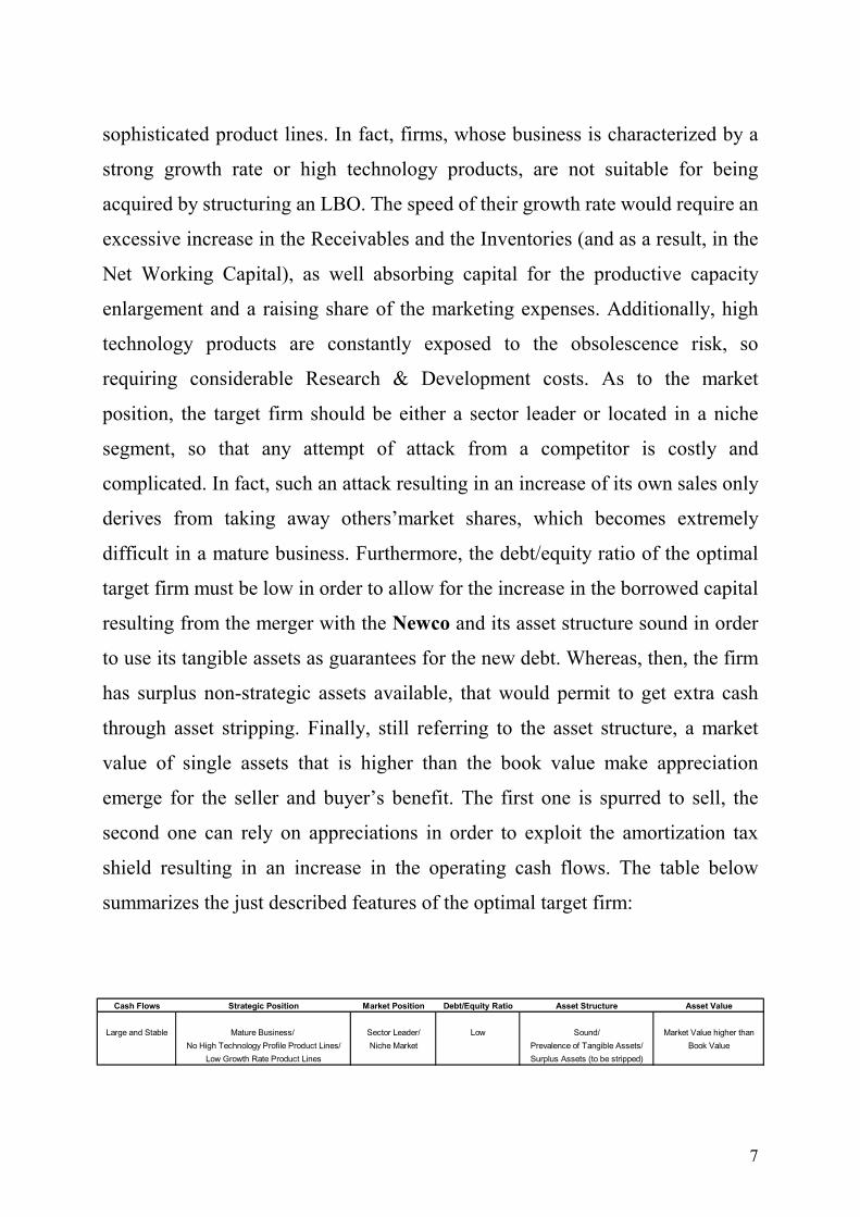
summarizes the just described features of the optimal target firm:

Cash Flows Strategic Position Market Position Debt/Equity Ratio Asset Structure Asset Value

Large and Stable Mature Business/ Sector Leader/ Low Sound/ Market Value higher thanNo High Technology Profile Product Lines/ Niche Market Prevalence of Tangible Assets/ Book Value

Low Growth Rate Product Lines Surplus Assets (to be stripped)

7

The valuation of the target firm of a leveraged buy-out is usually

accomplished by applying the Adjusted Present Value method (APV), which is

an hybrid “equity side” discounted cash flow method, as it is a combination of

the asset side and equity side approaches of the financial methodology for firm

valuation. The APV method, in fact, contains some of the elements that are

typical of the asset side and some others pertaining to the equity side. The

Adjusted Present Value of a given firm is the sum of two components: 1) the

value of the unlevered firm, which is estimated by discounting the Free Cash

Flows from Operations generated along the explicit forecast period at the

unlevered cost of equity (Ke) and adding to it a conveniently discounted

Terminal Value for the synthetic part of the forecast period; 2) the present value

of the interest tax benefits deriving from the use of a certain amount of debt. As

the firm is assumed to be unlevered (only equity-financed), it follows that the

value of the unlevered firm is an enterprise value also coinciding with an equity

value, since, according to the accounting relation Enterprise Value = WE + Debt,

there is no debt to be added. As a result, the final Adjusted Present Value of the

firm still remains an enterprise value, even after computing the present value of

the expected fiscal savings. It ends up representing the enterprise value of a

levered firm.

According to the known formula, the Adjusted Present Value of the firm

is computed as follows:

Wassets = WU + WTS

where:

Wassets = enterprise value (value of operating assets);

8

WU = value of the unlevered firm;

WTS = value of the fiscal benefits referred to borrowing (G, tax shield).

More specifically, the value of the levered firm (WL) can be unbundled in the

following parts:

(1 + Ke)Σ t

Kd x Dt x tc(1 + Kd)t = 1

n

WL = Wassets = Σ FCFOt = 1

n

+t

t TV(1 + Ke)n

n+ +

TV (G)(1 + Kd)

nt

WU = Enterprise Value G = Present Value of Tax Shield

(1 + Ke)Σ t


n

WL = Wassets = Σ FCFOt = 1

n

+t

t TV(1 + Ke)n

n+ +

TV (G)(1 + Kd)

nt

WU = Enterprise Value G = Present Value of Tax ShieldWU = Enterprise Value G = Present Value of Tax Shield

where:

FCFOt = free cash flows from operations at each time t;

Ke = unlevered cost of equity;

TVn = terminal value of the firm at time n;

Kd = cost of debt;

Dt = debt amount;

tc = tax rate;

TV (G)n = terminal value of the interest tax benefits.

The Adjusted Present Value becomes an equity value, when the present value of

debt (D) is subtracted from the enterprise value (Wassets):

9

Wequity = Enterprise Value (Wassets) - D

With regard to the Terminal Value, it expresses the value of the firm at the

end of the period of explicit forecast of cash flows. The methodologies that may

be used for its determination are those typical of the Analytic Financial Methods

with Terminal Value: Perpetual Growth Rate Method and Exit Multiples’

Method1. The former uses the Gordon’s synthetic formula, under the hypothesis

that the firm which is being valued, once reached a definite capacity of

producing cash flows, can grow indefinitely at the rate g. In the case of an

acquisition with a leveraged buy-out, the recourse to the variation of this

method, which assumes that the firm is in a situation of equilibrium

characterized by absence of growth, is excluded, since the firm in question has

become the target of the deal just because of its capacity of stable growth over

the time. The latter method, instead, bases the calculation of the Terminal Value

on the use of market multiples such as the EV\EBIT (Enterprise Value\Earnings

Before Interests and Taxes) in the assets side approach, assuming that the

Terminal Value, being a fraction of the firm’s value, may likewise be expressed

in function of the multiples which are implicit in comparable firms. Hence, let

us illustrate how to compute the Terminal Value with the Perpetual Growth Rate

Model, since such a method will be later applied in the proposed business case.

The Terminal Values that are involved in the Adjusted Present Value, TVn and

TV (G)n, are calculated as follows:

1 Given the reduced, if not almost inexistent, probability of a pay-off of the target firm’s assets in the operating

context of a LBO, the recourse to the liquidation value method , as a means for the estimate of the Terminal

Value, seems not to be admitted.

10

TV =n (Ke - g)

FCFO nTV =n (Ke - g)

FCFO n

nTV (G) =n (Kd - g)

FCFO nTV (G) =n (Kd - g)

FCFOTV (G) =n (Kd - g)

FCFO

where:

FCFO n = normalized average free cash flow from operations (to be considered

“in force” over the synthetic forecast period);

g = growth rate of the free cash flow from operations (namely, the firm’s

growth) over the synthetic forecast period.

It can be noticed that the cost of debt (Kd) is used to discount all the

cash flows related to the fiscal benefits (interest tax shield and Terminal Value).

Such a choice is attributed to the consideration that the riskiness of those cash

flows is well reflected in the average cost of debt, as tax shields are as uncertain

as principal and interest payments. Nevertheless, some others regard the use of

such a discount rate for the estimate of the present value of the interest tax

savings as being a significant drawback of the method, besides the computation

of the shareholders’ rate of return for the cash flows of the unlevered firm (the

11

unlevered cost of equity), since the APV does not find a solution to one of the

main disadvantages of the Adjusted WACC approach2.

The Adjusted Present Value method presents two important virtues:

1. it provides disaggregated information about the factors that

share in creating the firm’s value;

2. it permits a detailed analysis of the value deriving from the

choice of a particular financial structure by isolating the

contribution of fiscal benefits to the corporate value creation.

With regard to the latter beneficial feature, the APV can rely on the law of

preservation of, according to which the irrelevance of fiscal benefits connected

to the use of debt is equivalent to the absence of taxation within the first part of

the valuation leading to the determination of the value of the unlevered firm.

Hence - thanks to the transmission effects that operate from the asset value to

the discount rate – it follows the independence of the Weighted Average Cost of

Capital, which is applied to discount back the operating cash flows, from the

firm’s financial structure and the connected possibility of utilizing it in the place

of the unlevered cost of equity without distinction. That accounts for the use of

the cost of equity in the discounting process related to the unlevered firm

valuation.

2 The Adjusted WACC approach is the discounted cash flow method that is used alternatively to APV when the main goal is to put in evidence the value creation deriving from the exploitation of fiscal benefits. As to the main disadvantages of the Adjusted WACC approach, they are specifically referred to the miscalculation of the Weighted Average Cost of Capital. The errors usually made are the recourse to the targeted capital structure instead of the outstanding debt/equity ratio in the cost of equity’s computation and to book values instead of market values in the determination of the weights.

12

3. The expansion of the Adjusted Present Value of the target firm: the

valuation of a leveraged buy-out by means of the Real Options Approach

We have described how the equity value of the target firm can be found by

applying the Adjusted Present Value method. Such an equity value may be

compared to a passive Net Present Value (NPV), since the theoretical roots are

common between the NPV analysis and the Discount Cash Flow methodology.

As a result, we can name such an equity value as the “passive equity value”

(Passive Wequity) of the target firm. The conventional valuation does not capture

the flexibility of the managerial actions that can be performed in order to

influence the dynamics of the firm value. The informative set that the decision-

making rule of the Discounted Cash Flow methodology typically incorporates is

a static one, as both the business plan’s projections and the discounting process

rely on the information available at time zero. The passive equity value the APV

user gets to is a precommitted value which does not exploit the benefits of

managing and properly reacting to uncertainty. Such an uncertainty is, instead,

taken into account by the Real Options Analysis. What we intend to suggest is,

therefore, the expansion of the traditional valuation of a leveraged buy-out’s

target firm by applying Real Options. To accomplish this, we expand the

Adjusted Present Value as the equity value of the levered firm by integrating

such a passive equity value with the pricing of two real options that characterize

the operating context within which a leveraged buy-out is carried out. So it is

possible to convert the passive equity value into an equivalent expanded value

and transform the valuation of the firm that is being acquired from passive to

dynamic through the merger, in the process of managerial choices and thus, also

in the estimative process, of real options. The result of the suggested integration

is called Expanded Equity Value and may be got in the following way:

13

Expanded Equity Value (Expanded Wequity) =

= Passive Wequity + Real Option Value

Then, the Expanded Equity Value deriving from the Real Options Analysis of a

leveraged buy-out can be compared to the equity value of the target firm that is

obtained by means of the Adjusted Present Value method in order to appreciate

the value enhancement power incorporated in the former approach.

In detail, the subjects that carry out a leveraged buy-out have two real

options at their disposal in structuring the deal: a financial default option and an

operating default option. They are two options inherent in a LBO technique

itself that, considered together, form a compound option, since, as we are going

to see, only the exercise of the former gives the possibility to exercise the latter.

Particularly, such a compound option belongs to the category of the sequential

compound options, as the second option is created only when the first option is

exercised.

The financial default option permits to value an investment project

or a firm characterized by the recourse to borrowing by incorporating the

possibility of the financial default of debt into the valuation. Let us consider a

firm that borrows over the equity whose value must be determined. An

obligation for the shareholders of such a firm is paying back the contracted debt

on pain of default and the possibility for creditors of attacking the shareholders’

assets. The chance of resorting to bankruptcy transforms the shareholders’

obligation into an option. According to the Black-Scholes 1973’ seminal paper,

such an option is represented by the equity of the levered firm itself. The firm’s

equity, in fact, can be regarded as a call option on the value of the firm, whose

exercise price is the face value of the firm’s debt (including principal and

interest) and whose maturity is the maturity of the debt. The value of such a call

14

option must give the value of the firm’s equity. Provided that the considered

firm is the target of an LBO, it is therefore leveraged and thus relying on the

accounting relation between enterprise value (EV) and equity value (WE)

according to which:

Wequity = Enterprise Value - Debt

the underlying risky asset is represented by the enterprise value of the levered

firm, that may be calculated via the Adjusted Present Value method, as:

(1 + Ke)Σ t


n

Wassets = EV = Σ FCFOt = 1

n

+t

t TV(1 + Ke)n

n+ +

TV (G)(1 + Kd)

nt(1 + Ke)

Σ tKd x Dt x tc

(1 + Kd)t = 1

n

Wassets = EV = Σ FCFOt = 1

n

+t

t TV(1 + Ke)n

n+ +

TV (G)(1 + Kd)

nt

Hence, the payoff of the call option replicates the above mentioned accounting

relation and its value gives the Adjusted Present Value of the firm computed as

its equity value (Wequity).

If we analyse a LBO structure, we can understand how the just described

option framework perfectly follows the managerial process that those who carry

out a leveraged buy-out have to face. At the very moment in which the buyer-

investor sets up a Newco and negotiates the debt with the banks (or issues

subordinated bonds on the financial market) he acquires the faculty of paying

back the contracted debt or – when the management of the business does not

permit the production over the time of Free Cash Flows from Operations

sufficient to a complete reimbursement - of declaring his own default. It is, of

course, an undesirable event, but nevertheless possible during the lifetime of a

15

leveraged buy-out, whose uncertainty can be managed with flexibility in order to

exploit the connected larger value creation.

Then, it is possible to write, on the enterprise value of the target levered

firm as underlying risky asset, a financial default call option of American type

whose payoff at T maturity date is:

ET = max [EVT – DT; 0 ]

Default is declared

Debt is reimbursed

where:

Variable of state: enterprise value of the target levered firm;

Strike price: present (face) value of debt (including principal and interest);

Maturity date: T (coincident with the payoff date of debt).

Over the course of a LBO post-merger phase until reaching time T, the

financial default American call option written on the firm’s enterprise value,

which is in the hands of the buyer - the current shareholder of the firm, and of

his management, is in the money if the Free Cash Flows from Operations are

large enough to assure at least the profitable remuneration of debt-holders each

year, which translates into an enterprise value of the target firm higher than the

face value of debt included the interests accrued during all its lifetime. Debt

plays the role of the option strike price, since it is a contractually known

quantity that may be defined on the negotiation of the borrowing soon after the

16

setting up of the Newco. The consideration of the present value of debt

(principal and interest), under the hypothesis of the call option being in the

money, implies the firm’s capacity of its total reimbursement. It follows the

expedience for the shareholder to exercise the option, which is equivalent to

have paid over the time the borrowed capital. The financial default option is, on

the contrary, out of the money if at time T the Free Cash Flows from Operations

produced by the firm’s core-business are not only insufficient to remunerate the

shareholders’ equity, but they are not even sufficient to pay back the debt. That

is reflected in an enterprise value of the levered firm lower than the value of the

debt (principal and interest) and compels the shareholder, who holds the option,

not to find its exercise profitable and to declare the firm’s default. Furthermore,

by choosing the enterprise value of the levered firm computed via the Adjusted

Present Value method as the underlying risky asset of the financial default

option, its payoff is allowed to incorporate the value created by the exploitation

of the tax shield that is typical of a leveraged buy-out deal.

An operating default option is the other real option that comes out in the

course of the realization of a leveraged buy-out and that, therefore, shall be

analysed in the valuation process of the target firm. It is an option that, in the

case of an investment project, permits management to differ over the time the

repayment of the capital outlay needed for carrying out the project itself in

function of the Free Cash Flows from Operations gradually generated by the

firm’s core-business. The operating default option belongs, then, to the category

of deferral options.

In structuring an LBO, a wide range of managerial actions can be carried out

with the purpose of strengthening the business performance in order to reach a

more certain and rapid reimbursement of the borrowed capital. These

managerial actions, that are usually performed after the merger between the

Newco and the target firm, may be divided in extraordinary and ordinary

17

management interventions. The first ones are related to the dismissal of non-

strategic assets (asset stripping), while the second ones embrace the firm’s key

functional areas. Particularly, they can be concerned with the improvement of

the performance of the firm’s management and personnel, the production

structure, the commercial relations’ area (clients and providers), the product

strategy and the financial management. All these post-merger restructuring

actions require financial resources in order to be carried out.

Let us assume that after the merger the buyer-investor intends to perform

two ordinary management interventions: the innovation of the target firm’s

products and the improvement of commercial relations. More specifically, the

first intervention aims at influencing the characteristics of the firm’s offer. It is

not just a question of increasing the production capacity, but above all of

improving the characteristics of desirability of the product. The elevation of the

technological content of the offer, the reduction of the time threshold of the

product obsolescence or, more generally, any interventions aimed at acting on

the dimension of the firm’s product mix may contribute to it. In fact, a firm’s

product mix presents four principal dimensions: width, length, depth, and

consistency. They constitute the tools to define the corporate product strategy.

The width of the product mix measures the number of the different product

lines3 existing in the firm and put up for sale. Management can decide to add

new lines, widening the product mix. Instead, the product mix length is referred

to the total number of the products offered by the firm. Management can decide

to lengthen the lines of products in order to attract customers with different

tastes and needs. The product mix depth is its size with regard to the versions of

every product of the line. New versions may be added to every product and, in

this way, making the product mix deeper. Finally, the consistency of the product 3 A product mix is composed of different lines. A product line is a group of products closely connected, since

they carry out the same function, they are sold to the same customer category through the same commercial

outlets or they belong to the same price class.

18

mix measures the correlation degree among the different lines of products with

reference to their final use, the characteristics of the production process,

distribution channels etc.. Management can make the product mix more or less

consistent according to the aim of acquiring a strong reputation in a single sector

(for example, the historical one of the firm) or rather of entering a multiplicity of

sectors.

Let us assume that, besides the debt used to compose the financial

structure of the Newco, management resorts to a further borrowing to be repaid

in two different tranches (as explained later, the first of the tranches must be

paid at year 1 and the second one at year 2) in order to carry out the intervention

of product strategy (being the action related to commercial relations an indirect

cash-free effect of product innovation). Whatever the form taken by the latter,

the target firm’s management may need to regulate over the time the financial

outlay connected to its implementation waiting for the examination of the cash

flows from operations that the core business will be able to generate. This task

will be performed by the operating default call option, that, being of American

type, presents the following payoff at the maturity date T1 and can be exercised

at any time (as we will explain later, at predetermined decision nodes) during its

life:

ET1 = max [EVT1 – IT1; 0]

Operating default is declared

Investment payment is completed

19

where:

Variable of state: enterprise value of the target levered firm;

Exercise price: value of the second tranche of the borrowed capital necessary for

the carrying out of the investment project;

Maturity date: T1 (preceding T and coinciding with the maturity of the second

tranche of the borrowed capital).

At date T1 the exercise of the operating default call option suits the target

firm’s shareholders if it is in the money, that is if the Free Cash Flows from

Operations are produced in a quantity sufficient to assure the continuation of the

intervention of product innovation, which is reflected on the enterprise value of

the target firm higher than the debt share that has still to be paid. If, on the

contrary, the Free Cash Flows from Operations have finished their capacity of

reimbursement, being the target firm’s enterprise value lower than the value of

the debt share that is still to be paid, the option is out of the money, and its

exercise is not profitable for the shareholder of the target firm. The latter, then,

is compelled to declare the firm’s operating default, which equates to exercising

the right of definitely interrupting the project of improving the offer. It means

that the project in question has operationally failed, and the firm must be content

with the product or the product mix already existing. The product strategy

project yet played an important role in recovering the steadiness of growth of the

target firm’s cash flows and assuring the repayment of the financial debt

originally related to the Newco’s capital structure. Its operating failure turns into

a financial failure as well. It follows that, if the operating default option is left

unexercised, the buyer cannot aim at continuing the firm’s activity because all

the value creation initiatives originally targeted cannot operate. As a result, the

Free Cash Flows from Operations, that would have allowed to reimburse the

20

financial debt, will not be sufficient. If, instead, the operating default option is

exercised, the value, that will be creating over the years until the buyer’s way

out, may contribute to the final repayment of the financial debt and, therefore, to

repeatedly exercising the related financial default option. That would mean a

successful way out for the buyer-investor. Then, we understand how the

operating default comes before the possible financial default, leaves it aside and

does not exclude it.

A leveraged buy-out has in itself the two rights allowed to the shareholder

of which we said above. A financial default and an operating default are two

possible events in a firm’s lifetime and the consideration of the two categories of

options that are contingent on them accounts for the managerial flexibility,

which creates value only owing to the fact of permitting to make correct choices

and to take the relative decisions in the right moment. That eliminates the

passive and static quality peculiar to traditional valuation and makes it dynamic,

in keeping with the possible sources of value offered by the reality of firm

management.

Let us suppose that the setting up of the Newco necessary to carry out the

LBO needs an initial investment equal to I0E + I0D, that is equivalent to the

composition of its financial structure. The equity brought-in by the team of

buyers-investors (the new shareholders) is equal to I0E and the borrowed capital

negotiated with the banks and\or placed with the investors on the financial

market (bondholders) is equal to I0D.

The financial structure of the vehicle company destined to merge the target firm

is composed as follows:

I0E = equity

Newco’s capital structure

I0D = financial debt

21

The debt contracted by the firm is risky, so the applied interest rate (Kd) is

obtained by adding a risk premium (πD) to the risk-free rate (rf) for risk-less

investments. The financial debt expiration date is stated in time T5, coinciding

with the time chosen by the team of buyers-investors for the way out. It means

that the obligations taken by the firm’s new shareholders, that is the debt

reimbursement and the payment of relative interests, must be satisfied. If the

new shareholders do not fulfil their obligations and do not pay back the debt at

time T = t5 [D5 = I0D x (1+ Kd)5), the firm’s default will be declared and the

bondholders\banks will take possession of the corporate assets, they will carry

out the winding-up by getting the present value at time T = T5 (V5) and they will

pay back their credit, partially or totally, by means of what they obtain from the

winding-up. Let us assume, furthermore, that the management team of the target

firm, after the merger between the Newco and the target, may carry out the

product strategy by financing at the valuation date t0 the relative intervention in

two different tranches, the first equal to I1 to be paid at the end of the merger

deal, at the beginning of period t1 and the second to be disbursed a year later at

the beginning of period t2 and whose value (principal and interest) is equal to I2.

The form of borrowing that management may choose in order to finance the

intervention of ordinary management related to the firm’s output is a short-term

debt. As it was outlined above, the carrying out of a leveraged buy-out and its

conduct create intrinsically the two real options of financial and operating

default that may be represented with this pattern:

FINANCIALDEFAULTOPTION

Exercise Price = D5

T = t5

OPERATINGDEFAULT

OPTION

Exercise Price = I2

T1 = t2

FINANCIALDEFAULTOPTION

Exercise Price = D5

T = t5

OPERATINGDEFAULT

OPTION

Exercise Price = I2

T1 = t2

22

We can easily understand that the two real options form together a

compound option, since the decision to proceed to the acquisition by means of a

leveraged buy-out permits the buyer the discretionary exercise of a financial

default option. Still better, we can say that the choice itself of carrying out a

leveraged buy-out is a financial default option. It follows that, conceptually, the

operating default option is acquired by the buyer\shareholder of the target firm

only afterwards and because he had acquired the first right: the financial default

option. That accounts for compounding. Nevertheless, practically, the operating

default option is chronologically antecedent to the financial default option. The

type of compounding is sequential, as the time sequence of the real options

involved in an LBO is the opposite of their order of economic priority. The first

chronological option (the operating default option) is, in fact, the second option

from an economical point of view and the option that chronologically comes as

second (the financial default option) is the most important one in economical

terms.

The valuation process of the sequential compound option starts by

building the firm’s enterprise value tree. First, in fact, we evaluate the financial

default option, whose value in t0 corresponds to that one of the equity of the

levered firm under the APV hypothesis acting as an American call on the

enterprise value with its exercise price equal to the face value of debt (principal

and interest). Once we model the present enterprise value of the levered target

firm and its up and down movements by computing the relative standard

deviation, the uncertainty regarding the evolution of the operating cash flows

results in a recombining binomial event tree that becomes the underlying risky

asset for the financial default call option. The enterprise value tree of the firm is

illustrated in the figure 2:

23

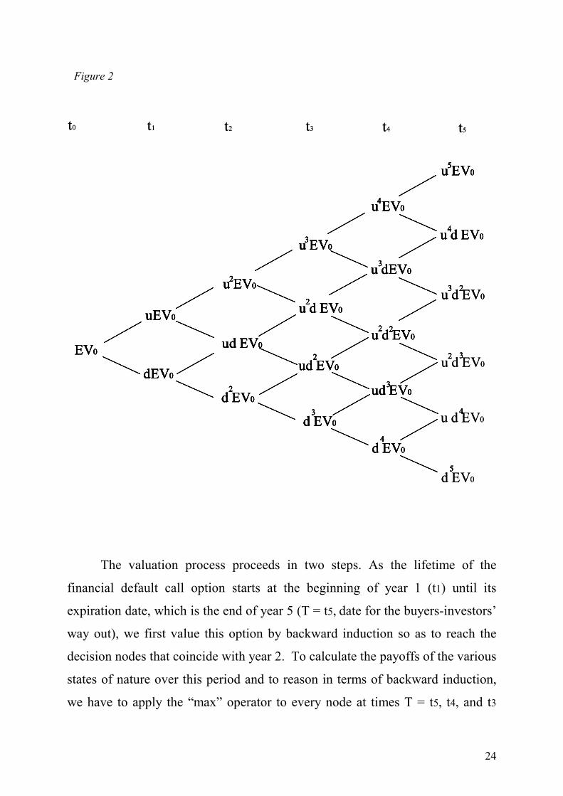
Figure 2

u d EV0

u d EV0

d EV0

u d EV0

u d EV0

EV0

dEV0

d EV0

uEV0

ud EV0

u EV02

2

u EV03

u d EV02

ud EV02

d EV03

u EV04

u dEV03

u d EV02 2

ud EV03

d EV04

u EV05

4

3 2

2 3

4

5

u d EV0

u d EV0

d EV0

u d EV0

u d EV0

EV0

dEV0

d EV0

uEV0

ud EV0

u EV02

2

u EV03

u d EV02

ud EV02

d EV03

u EV04

u dEV03

u d EV02 2

ud EV03

d EV04

u EV05

4

3 2

2 3

4

5

u d EV0

u d EV0

EV0

dEV0

d EV0

uEV0

ud EV0

u EV02

2

u EV03

u d EV02

ud EV02

d EV03

u EV04

u dEV03

u d EV02 2

ud EV03

d EV04

u EV05

4

3 2

2 3

4

5

u d EV0

EV0

dEV0

d EV0

uEV0

ud EV0

u EV02

2

u EV03

u d EV02

ud EV02

d EV03

u EV04

u dEV03

u d EV02 2

ud EV03

d EV04

u EV05

4

3 2

2 3

4

5

EV0

dEV0

d EV0

uEV0

ud EV0

u EV02

2

u EV03

u d EV02

ud EV02

d EV03

u EV04

u dEV03

u d EV02 2

ud EV03

d EV04

u EV05

4

3 2

2 3

4

5

t0 t1 t2 t4t3 t5t0 t1 t2 t4t3 t5

The valuation process proceeds in two steps. As the lifetime of the

financial default call option starts at the beginning of year 1 (t1) until its

expiration date, which is the end of year 5 (T = t5, date for the buyers-investors’

way out), we first value this option by backward induction so as to reach the

decision nodes that coincide with year 2. To calculate the payoffs of the various

states of nature over this period and to reason in terms of backward induction,

we have to apply the “max” operator to every node at times T = t5, t4, and t3

24

belonging to the binomial tree that draws the dynamics of the value of the

underlying (the stochastic process for the levered firm’s enterprise value under

the APV conditions). That transforms the enterprise value event tree into a

decision tree (figure 3).

Figure 3

Financial Default Option

EV0

dEV0

uEV0

2

2

3

2

2

3

4

3

2 2

3

4

max [u EV0 – D5 ; 0]5

2

3

max [u dEV0 – D5 ; 0]4

max [u d EV0 – D5 ; 0]3

max [d EV0 – D5 ; 0]5

max [u d EV0 – D5 ; 0]2

max [u d EV0 – D5 ; 0]4

max [u EV0 – D4 ; CV4]

max [u d EV0 – D4 ; CV4]



max [d EV0 – D4 ; CV4]





u EV0

ud EV0

d EV0

EV0

dEV0

uEV0

2

2

3

2

2

3

4

3

2 2

3

4

max [u EV0 – D5 ; 0]5

2

3

max [u dEV0 – D5 ; 0]4

max [u d EV0 – D5 ; 0]3

max [d EV0 – D5 ; 0]5

max [u d EV0 – D5 ; 0]2

max [u d EV0 – D5 ; 0]4










u EV0

ud EV0

d EV0

dEV0

uEV0

2

2

3

2

2

3

4

3

2 2

3

4

max [u EV0 – D5 ; 0]5

2

3

max [u dEV0 – D5 ; 0]4

max [u d EV0 – D5 ; 0]3

max [d EV0 – D5 ; 0]5

max [u d EV0 – D5 ; 0]2

max [u d EV0 – D5 ; 0]4










u EV0

ud EV0

d EV0

Operating Default Option

25

At all end nodes of year 5, we calculate the related payoffs and decide

whether the firm is able to repay its debt through the Free Cash Flow from

Operations that will be generated in the future or it will be forced to go

bankrupt. At all the five nodes of year 4, the continuation value of the American

financial default call option is compared to its present payoff in order to take the

optimal exercise decision. If the continuation value of the option is greater than

the payoff at the current node (that is, the value of the option unexercised

exceeds its value if exercised), then the firm’s activity is carried out and no

default is declared. It means that the Free Cash Flow from Operations still

maintain their capacity of debt reimbursement. On the contrary, if the

continuation value of the option is lower than the present node’s payout,

management makes the firm go bankrupt instead of keeping the financial default

option open. For the moment, let us leave aside the nodes related to years 0, 1

and 2.

The continuation value of the financial default call option may be calculated by

applying either the Replicating Portfolio Approach or the Risk-Neutral

Probability Approach (given their equivalence). If we choose to use the latter

methodology, we need to compute the risk-neutral probabilities to be utilized in

the valuation according to the known formula:

1 + rf – dq =

u – d=

m – du – d

1 + rf – dq =

u – d=

m – du – d

where:

m = 1 + rf

26

Probability q is the risk-adjusted probability of an upward trend. The probability

of the value of the underlying asset going into the low state of nature is simply

obtained by calculating the complement to 1 of q. We, then, apply the closed

pricing formula derived from the Cox-Ross-Rubinstein model to compute the

continuation value:

C = +1 + rfq Cu (1- q) Cd

1C = +1 + rfq Cu (1- q) Cd

1 +1 + rfq Cu (1- q) Cd

1

where:

C = continuation value of the American financial default call option (more in

general, value of the option at time 0);

Cu = payoff of the financial default call option in the up-state node;

Cd = payoff of the financial default call option in the down-state node.

Alternatively, we can use the Replicating Portfolio Approach, which is

equally derived from the Cox-Ross-Rubinstein model and relies on the law of

one price for assets providing the same payouts. Such a method consists in

building an hedged portfolio that is composed of one share (�) of the underlying

risky asset (twin security) and a short position in one or more units (C) of the

option that is being priced, so that the capital gain or loss from holding the twin

security will be perfectly offset by the correspondent capital loss or gain in the

short position created by writing one or more calls on such an underlying risky

asset. A simple algebraical inversion operation shows how the so composed

portfolio with a resulting hedge ratio is riskless, as its payoff is that one of a

risk-free bond (B):

27

� V0 – C0 = B0

� V0 + B0 = C0

Furthermore, we make the Marketed Asset Disclaimer assumption4 that

allows for the integrated and simultaneous use of the Replicating Portfolio

Approach and the Twin Security Approach, being the latter typically related to

the traditional Net Present Value analysis. In fact, such an assumption does

permit to avoid the search for a traded twin security by substituting it with the

pure NPV of the asset that is being valued, namely “without flexibility”.

The Replicating Portfolio Approach consists in equating the end-of-period

payoffs of the hedged portfolio in the two considered states of nature and in

finding a hedge ratio (�), that is chosen so that the portfolio will return the same

cash flows in either state of nature. The result will be a riskless portfolio:

{� ut Vt-1 + (1 + rf) B = Cu

� Vt-1 (ut – dt ) = Cu - Cd

� dt Vt-1 + (1 + rf) B = Cd{� ut Vt-1 + (1 + rf) B = Cu

� Vt-1 (ut – dt ) = Cu - Cd

� dt Vt-1 + (1 + rf) B = Cd

� ut Vt-1 + (1 + rf) B = Cu

� Vt-1 (ut – dt ) = Cu - Cd

� dt Vt-1 + (1 + rf) B = Cd

28

4 See Tom Copeland –Vladimir Antikarov, “Real Options. A Practitioner’s Guide”, 2001.

Cu - Cd

Vt-1 (ut – dt )� =

Cu - Cd

Vt-1 (ut – dt )� =

The law of one price allows for the pricing of the hedged portfolio and, hence,

of the option at each of the end-of-period nodes of the year before :

� Vt-1 + B = C

At the end of year 2, the operating default call option, that is written on

the enterprise value of the target levered firm and gives the buyer the right to

decide whether or not to carry out the product strategy project, expires. As

described above, if such an option is not exercised, it does not give the buyer the

right to proceed to manage the target firm by repaying the second tranche of the

short-term debt which finances the output improvement. That makes the

leveraged buy-out unsuccessfully terminate beforehand. More important, the

operating default option is not merely contingent on the target levered firm’s

enterprise value, but on the enterprise value incorporating the current value of

the financial default option (PV (CV)). Such a “flexible” enterprise value acts as

underlying risky asset of the operating default option expiring at year 2 of the

post-merger phase of the leveraged buy-out. The enterprise value of the target

firm, which includes the present value of the American financial default call

29

option acting from year 2 (t2) to year 5 (t5), is calculated by applying the

Replicating Portfolio Approach and needs to be compared to the operating

default option’s exercise price at the nodes of time t2. If the “flexible” enterprise

value of the firm is greater than the exercise price (I2), its business operations

continue and managers can rely on the gradual production of operational cash

flows to monitor the reimbursement of the financial debt. Such a monitoring

activity is performed by looking at the continuation value of the American

financial default option at the successive nodes of the binomial tree of the

underlying. Whereas the payout of the option is negative, the default of the

target firm is declared. Otherwise, if the enterprise value of the firm,

representing the continuation value of the American option, exceeds the face

value of the debt (principal and interests) until reaching the end-of-period nodes

of the binomial tree, meaning that the Free Cash Flows from Operations are

large enough along the predetermined lifetime of the deal to repay the borrowed

capital, the buyer can successfully execute the way out. The same backward

induction procedure is repeated for the year 1 node (t1), as the operating default

call option is of American type too and its present value is calculated in t0 (PV

(CV0)) (figure 4).

30

Figure 4

PV (CV0)

2

2

3

2

2

3

4

3

2 2

3

4

max [u EV0 – D5 ; 0]5

2

3

max [u dEV0 – D5 ; 0]4

max [u d EV0 – D5 ; 0]3

max [d EV0 – D5 ; 0]5

max [u d EV0 – D5 ; 0]2

max [u d EV0 – D5 ; 0]4










max [PV (CVu ) – I2 ; 0]

max [PV (CVud ) – I2 ; 0]

max [PV (CVd ) – I2 ; 0]

max [PV (CVu ) – I2 ; 0]

max [PV (CVd ) – I2 ; 0]

PV (CV0)

2

2

3

2

2

3

4

3

2 2

3

4

max [u EV0 – D5 ; 0]5

2

3

max [u dEV0 – D5 ; 0]4

max [u d EV0 – D5 ; 0]3

max [d EV0 – D5 ; 0]5

max [u d EV0 – D5 ; 0]2

max [u d EV0 – D5 ; 0]4










max [PV (CVu ) – I2 ; 0]

max [PV (CVud ) – I2 ; 0]

max [PV (CVd ) – I2 ; 0]

max [PV (CVu ) – I2 ; 0]

max [PV (CVd ) – I2 ; 0]

Even though, in fact, the American financial default call option only

operates from the end of the year 2, its lifetime must be considered throughout

the deal from time t0 to time t5 in order to estimate the present value of the

compound option. Therefore, the enterprise value event tree that is illustrated in

the figure 4 must be continued until the time 0 (t0) by computing the

continuation value of the American financial default call option and comparing

it to its current node’s payoff. That gives us the value of the financial default

option at the valuation date (figure 5).

31

Figure 5

2

2

3

2

2

3

4

3

2 2

3

4

max [u EV0 – D5 ; 0]5

2

3

max [u dEV0 – D5 ; 0]4

max [u d EV0 – D5 ; 0]3

max [d EV0 – D5 ; 0]5

max [u d EV0 – D5 ; 0]2

max [u d EV0 – D5 ; 0]4











max [ud EV0 – D2 ; CV2]




PV (ET0)

2

2

3

2

2

3

4

3

2 2

3

4

max [u EV0 – D5 ; 0]5

2

3

max [u dEV0 – D5 ; 0]4

max [u d EV0 – D5 ; 0]3

max [d EV0 – D5 ; 0]5

max [u d EV0 – D5 ; 0]2

max [u d EV0 – D5 ; 0]4















2

2

3

2

2

3

4

3

2 2

3

4

max [u EV0 – D5 ; 0]5

2

3

max [u dEV0 – D5 ; 0]4

max [u d EV0 – D5 ; 0]3

max [d EV0 – D5 ; 0]5

max [u d EV0 – D5 ; 0]2

max [u d EV0 – D5 ; 0]4















PV (ET0)

By doing so, it is now possible to compare the enterprise value incorporating the

current value of the financial default option (PV (CV0)), acting as the

continuation value of the operating default option, to the present value of the

financial default option (PV (ET0)). The first value, if greater than the second

one, corresponds to the profitable continuation of the operating default call

option towards the successive nodes, while the second value, if greater than the

first one, coincides with the profitable exercise of the operating default option.

In the latter case, in fact, the exercise of the operating default option –

conceptually - gives an immediate start to the financial default option. Whatever

the value is chosen, that is, whether the operating default option is continued or

exercised, the value of the compound option, as determined in t0, identifies what

32

we are referred to as the Expanded Equity Value (Expanded Wequity) of the target

firm. As already explained, such a value realizes the expansion of the

conventional equity value as computed by means of the Adjusted Present Value

method, being the payoffs of both the real options involved structured as the

difference between the enterprise value of the levered firm and the present value

of debt. Thus, the Expanded Equity Value of the target firm incorporates the

value of the compound option, as sequentially composed by the operating

default call option and the financial default call option, that is added to the

passive equity value:


= Passive Wequity + Compound Option Value =

= Passive Wequity + Operating Default Option Value +

+ Financial Default Option Value

Having computed the Expanded Equity Value of the target firm by means

of the Real Options Approach, we can easily extract the value of the compound

option by subtracting the passive equity value from the Expanded Equity Value

itself. Since:

Expanded Equity Value ( Expanded Wequity) - Passive Wequity =

Compound Option Value

33

Such a calculation permits to estimate the contribution that the integrated use of

the Real Options Analysis brings into the valuation of the target firm of an LBO.

We can conclude that the appraisal process of the target firm of a

leveraged buy-out through the Real Options Analysis, if compared to that one

based on the Adjusted Present Value method, presents the following two

advantages:

1. it captures the managerial flexibility of the firm value uncertainty, which

is not included in the passive and static Adjusted Present Value;

2. it continues to incorporate the extra-value created by the exploitation of

the tax shield, as the APV method does, since the underlying risky asset

of the compound option is the enterprise value of the levered firm

including the present value of the fiscal benefits.

4. Business Case: the valuation of Chemical Brothers SpA

Chemical Brothers SpA is active in the sector of disposal and reconversion of

waste products. More specifically, it operates in the following two business

segments:

�� the recovery, purification and production of organic solvents;

�� the production of fine pharmaceutical intermediates.

The first business unit collects any kind of industrial liquid waste product in

order to treat and recover it by means of purification processes. By purifying and

fractioning heterogeneous mixtures, different types of solvents are extracted,

fractionated and dehydrated for re-use in their original processes. All the by-

products obtained from processing are analysed for possible commercial use or

are treated as waste for later disposal. Chemical Brothers’ revenues in this

34

business segment derive from the solvents’ sale to the same main firms from

which are originally collected (chemical, petrochemical, pharmaceutical,

engineering firms), as well as from the waste collection. The result of the

organic solvents’ treatment by this business unit of Chemical Brothers is as

follows:

- 70% recovered as solvents to be sold to the market;

- 20% transformed in distilled water to be eliminated;

- 10% concentrated waste to be eliminated.

The second business unit exploits the same technological know-how that

is employed in the first business unit in order to produce pharmaceutical

intermediates through a synthesis process regarding raw materials acquired by

third parties.

In the year 2003, Chemical Brothers recorded revenues for € 48.4 million

and has a current production capacity of about 150.000 tons per year of

industrial solvents with an authorization to treat 98.900 tons of industrial

solvents per year. Capital expenditure in the coming years is expected to be

limited, since the firm has made significant investments in the past years (its

plants are considered among the most technological advanced for organic

solvents’ treatment).

The current shareholders propose a family buy-out through the sale of a

majority stake to a financial partner in order to continue the business

development and to prepare Chemical Brothers for an IPO/trade sale in the next

5 years. Shareholders will retain a minority stake (30%) in the firm, as well as

the management positions. The leveraged buy-out is executed in December 2003

and the way out is expected for the year 2008.

35

The Pro Forma Income Statements and the Pro Forma Balance Sheets

resulting from the transaction proposed by the buyer-investor are illustrated in

figure 6:

Figure 6

Pro Forma Income Statements 2003 2004E 2005E 2006E 2007E 2008E(in thousands of Euro)

EBIT 6.046 11.090 16.264 17.935 19.009 19.914 Interest 1.013- 1.747- 1.434- 1.043- 520- 5- EBT 5.033 9.343 14.830 16.892 18.489 19.909 Taxes (35%) 1.762- 3.270- 5.191- 5.912- 6.471- 6.968- Net Income 3.271 6.073 9.640 10.980 12.018 12.941

Supplemental Data

Depreciation 3.451- 2.874- 2.126- 1.738- 1.847- 1.908- Capex 6.096- 2.000- 2.000- 2.000- 2.000- 2.000- Change in NWC 3.480 3.038- 2.835- 1.145- 953- 976- Change in other assets/liabilities 3.239- 3.130 1.456- 582 130- 216

Pro Forma Balance Sheets 2003 2004E 2005E 2006E 2007E 2008E(in thousands of Euro)Net Working Capital 10.720 13.758 16.593 17.738 18.691 19.667 Net Fixed Assets 40.604 39.730 39.604 39.866 40.019 40.111 Other Assets/Liabilities 1.351- 4.481- 3.025- 3.607- 3.477- 3.693- Net Capital Employed 49.973 49.008 53.172 53.997 55.234 56.086

Overdraft/(Cash) 11.452 10.413 8.938 2.783 3.999- 12.087- Short Term Debt 2.000 - - - - - Senior Debt 20.000 16.000 12.000 8.000 4.000 - Mezzanine Debt 5.000 5.000 5.000 5.000 5.000 5.000 Total debt 38.452 31.413 25.938 15.783 5.001 7.087- Equity 11.521 17.595 27.234 38.214 50.232 63.173 Total Sources 49.973 49.008 53.172 53.997 55.234 56.086

36

The buyer-investor designs the financial strategy that underlies the

leveraged buy-out so as to have the Newco’s capital structure composed by a

77% of debt and a 23% of equity. Particularly, the debt consists of four different

forms of borrowing: the revolving credit facility (€ 11.4 million), which is used

to finance the Net Working Capital; the short-term debt (€ 2 million, second

tranche), which acts as a bridge financing from the LBO’structuring year (2003)

to the merger’s year in order to fund the proposed intervention of product

innovation; the senior debt (€ 20 million), that usually represents the largest

portion of the leverage ratio in a leveraged buy-out and is amortised in five years

through the payment of an annual costant instalment of Euro 4 million; the

mezzanine debt (€ 5 million), structured as a bullet bond with an equity kicker,

which gives a warrant to its holders for the purchase of an equity stake of the

target firm upon the way out. The resulting Net Financial Position is equal to €

38.4 million against a pre-merger one amounting to € 18.7 million, being the

shareholders’ equity equal to € 31.3 million (equity = 63%; debt = 37%). The

figure 7 shows the income statements and the balance sheets that would have

been projected over the future life of the firm if it had not been the target of an

LBO:

37

Figure 7

Pro Forma Income Statements 2003 2004E 2005E 2006E 2007E 2008E(in thousands of Euro)EBIT 6.046 6.840 12.750 14.197 15.241 15.038 Interest 1.013- 758- 492- 190- 24- 69- EBT 5.033 6.082 12.259 14.007 15.217 14.969 Taxes (35%) 1.762- 2.129- 4.291- 4.902- 5.326- 5.239- Net Income 3.271 3.953 7.968 9.104 9.891 9.730

Supplemental DataDepreciation 3.451- 2.874- 2.126- 1.738- 1.847- 1.908- Capital Expenditure 6.096- 2.000- 2.000- 2.000- 2.000- 2.000- Change in Net Working Capital 3.480 935- 3.015- 977- 896- 355- Change in other Assets/Liabilities 3.239- 3.130 1.456- 582 130- 216

Pro Forma Balance SheetNet Working Capital 10.720 11.655 14.670 15.647 16.543 16.898 Net Fixed Assets 40.604 39.730 39.604 39.866 40.019 40.111 Other Assets/Liabilities 1.351- 4.481- 3.025- 3.607- 3.477- 3.693- Net Capital Employed 49.973 46.904 51.250 51.906 53.085 53.316

Net Financial Position 18.669 11.646 8.024 424- 9.136- 18.635- Equity 31.304 35.258 43.226 52.330 62.221 71.951 Total Sources 49.973 46.904 51.250 51.906 53.085 53.316

To make the structuring of the leveraged buy-out profitable and enhance

the target firm’s performance in terms of generation of Free Cash Flows from

Operations, the buyer-investor chooses to resort to two different interventions of

post-merger ordinary management regarding the product strategy and the

commercial relations area. The benefits of the first of these interventions are

partially offset by a negative effect on the firm’s financial management. Both

the value creation initiatives aim at causing an EBIT improvement. The first

action, which is financed with a short-term debt, enhances the technological

content of the products provided by the organic solvents’ business unit. Such an

innovation action justifies a price increase and, hence, the Chemical Brothers’

revenues are expected to grow because of the two virtuous effects on sales’

volumes and prices. Such an intervention also determines an undirect effect on

the commercial relations’ side. By relying on greater sales’ volumes, in fact,

management can get a discount on the costs of raw materials from the firm’s

38

main providers. More in detail, the incidence of raw materials’ costs on revenues

decreases from 24% to 22%. It results that both these actions cause an EBIT

increase. Nevertheless, the revenues’ growth produces an increase in the Net

Working Capital, as, under the same conditions allowed to clients, Receivables

and Inventories are also due to grow. The related cash absorption partially

counterbalances the positive effects that are determined by an EBIT increase on

the production of Free Cash Flows from Operations. The calculation of the

operating cash flows shows what is mentioned above (figure 8):

Figure 8

Pro Forma Cash Flow 2003 2004E 2005E 2006E 2007E 2008E(in thousands of Euro)EBIT 6.046 11.090 16.264 17.935 19.009 19.914 Taxes 1.762- 3.270- 5.191- 5.912- 6.471- 6.968- EBIT (1-T) 4.284 7.820 11.073 12.023 12.538 12.946 Depreciation 3.451 2.874 2.126 1.738 1.847 1.908 Operating Cash Flow 7.735 10.694 13.199 13.761 14.385 14.854 Change in Net Working Capital 3.480 3.038- 2.835- 1.145- 953- 976- Capital Expenditure 6.096- 2.000- 2.000- 2.000- 2.000- 2.000- Other Assets/Liabilities 3.239- 3.130 1.456- 582 130- 216 Free Cash Flows from Operations 1.880 8.785 6.909 11.198 11.301 12.094

We now have to calculate the Adjusted Present Value of the target firm.

The estimate is based on the following assumptions and computations regarding

the cost of equity and the cost of debt:

Tax Rate 35,0%Growth Rate 0,0%Risk Free Rate 4,4%Target Debt/Equity Ratio 60%Unlevered Beta 0,56Equity Risk Premium 5,4%Unlevered Cost of Equity 9,8%Cost of Debt 5,0%

39

The Adjusted Present Value is calculated in two steps. The first step

consists in discounting back to 2003 for five years the unlevered operating cash

flows and the Terminal Value at the unlevered cost of equity of 9,8%. The value

we get to is the enterprise value of the target firm:

Post LBO ValuationPV of Free Cash Flows from Operations 34.331 PV of Terminal Value 70.414 Enterprise Value 104.745

The second step is concerned with the computation of the present value of the

tax shield by discounting back the fiscal benefits and their Terminal Value in the

year 2008 at the cost of debt (5,0%):

Interest Tax Shield 2003 2004E 2005E 2006E 2007E 2008EInterests 1.013 1.747 1.434 1.043 520 5 Tax Shield 355 611 502 365 182 2 Discount Rate 5,0%PV of Tax Shield 1.770 PV of Terminal Value 27 Total Present Value of Tax Shield 1.797

By adding the enterprise value and the present value of the interest tax shield,

we obtain the Adjusted Present Value of the target firm, which represents the

enterprise value of the levered firm itself:

APVEnterprise Value of the Levered Firm 104.745 PV of Interest Tax Shield 1.797 Total 106.542

40

If we want to estimate the equity value of the firm in terms of APV, we only

need to subtract the present value of debt from the enterprise value, according to

the known formula:

Wequity = Enterprise Value (Wassets) - D

= 106.542 – 38.452 = 68.090

Finally, if we want to highlight the contribution to corporate value

creation of the business iniatitives carried out by the buyer-investor, we can start

from the valuation of the target firm on the basis of the seller’s plan (which does

not include the execution of the leveraged buy-out) and get to the Adjusted

Present Value by providing evidence of the contributive effects of each of the

proposed managerial actions (figure 9):

41

Figure 9

Pro Forma Cash Flow 2003 2004E 2005E 2006E 2007E 2008E(in thousands of Euro)EBIT 6.046 6.840 12.750 14.197 15.241 15.038 Taxes 1.762- 2.129- 4.291- 4.902- 5.326- 5.239- EBIT (1-T) 4.284 4.711 8.460 9.294 9.915 9.799 Depreciation 3.451 2.874 2.126 1.738 1.847 1.908 Operating Cash Flow 7.735 7.585 10.586 11.032 11.762 11.707 Change in Net Working Capital 3.480 935- 3.015- 977- 896- 355- Capital Expenditure 6.096- 2.000- 2.000- 2.000- 2.000- 2.000- Other Assets/Liabilities 3.239- 3.130 1.456- 582 130- 216 Free Cash Flows from Operations 1.880 7.780 4.115 8.638 8.736 9.568 PV of Free Cash Flows from Operations 27.414 PV of Terminal Value 55.574 Unlevered Firm Value 82.987

Value Creation Initiatives and Negative Effects:

EBIT improvement

Incremental EBIT - 4.250 3.513 3.739 3.768 4.876 Taxes - 1.487 1.230 1.309 1.319 1.707 Cash increment After Tax - 2.762 2.284 2.430 2.449 3.169 PV of Annual Cash Increments 9.032 PV of Terminal Value 18.455 Total PV 27.487

Net Working Capital Increase - 2.103- 181 168- 58- 621- PV of Annual Cash Increments 2.114- PV of Terminal Value 3.615- Total PV 5.729-

Adjusted Present Value of the Target Firm 104.745

As mentioned above, our aim is to show how the “Discounted Cash Flow”

paradigm, which also includes the Adjusted Present Value methodology, is

flawed and systematically underestimates the value of firm. We, then, proceed to

perform a challenging valuation of the Chemical Brothers SpA by applying the

Real Options Approach, as described in the second part of this paper.

First, we start from the Adjusted Present Value of the target levered firm,

computed as enterprise value, which has to be subjected to the expansion via the

use of real options. Such an enterprise value (€ 106.5 million) identifies the

starting point of the related binomial event tree.

Second, we draw the dynamics of the enterprise value of the levered firm,

acting as the underlying risky asset of the real options to be priced, by

calculating the up and down movements along the binomial tree. To accomplish

this, we need to identify the driver of uncertainty that makes, through the Free

42

Cash Flows from Operations, the enterprise value of the target levered firm the

variable of state of the model. We assume that such an uncertainty driver is only

represented by market uncertainty. We, then, exclude technical uncertainty,

being such form of riskness the other potential driver of the evolution of a real

option’s underlying. Market volatility is composed by three different forms of

uncertainty which influence the firm’s Earnings Before Interests and Taxes

(EBIT):

- price uncertainty;

- demand uncertainty;

- variable cost uncertainty.

By analysing the Chemical Brothers’s business, we decide that, as well as

considering variable cost uncertainty, price uncertainty and demand uncertainty

can be well reflected and, thereby, consolidated in revenues uncertainty. Then,

we decide to apply two different approaches in order to get the volatility of the

target firm’s enterprise value: a linear regression capturing the influence of

revenues and variable costs on EBIT and a management assumption approach.

The first one aims at computing volatility by comparing the target firm’s results

to the overall performance of its economic sector. Therefore, such an approach

is constructed as an objective one. On the contrary, the second approach

represents a more standard volatility estimation method in the Real Options

Analysis and also a more involving one, as it is based on the management’s

assumptions. By comparing these two approaches, we obtain a very similar

result, which supports the use of the volatility figure in our calculations.

With the first approach, we exploit the influence of revenues and variable

costs (being these costs represented by raw materials’ costs) on EBIT by

estimating a regression of the former on the latter. The regression equation is the

following:

43

y = revenues a1 + raw materials costs a2 + ε

The sample of the regression is composed by 60 firms (including the Chemical

Brothers SpA) located in Lombardia (Italy) and belonging to the sector of

collection and disposal of solid waste. The data used for the regression have

been extracted from the 2001 financial reports of the firms. We find that

revenues explain the EBIT generation for 99,3% and, as expected, the

coefficient sign of raw materials’ costs is negative. The table below shows the

estimate of the regression equation:

95% Confidence Interval for CoefficientsModel Coefficients t Lower Bound Upper Bound

constant -3,538 -3,828 -5,388 -1,687a1 1,127 8,129 0,849 1,404a2 -0,117 -1,419 -0,283 0,048

Market volatility has been calculated by taking the arithmetic mean of the upper

and lower bounds of the 95% confidence interval of the significant coefficient of

the regression (0,849 and 1,404) and this gives a � equal to 1,1%.

The second approach to estimating volatility also relies on revenues and variable

cost uncertainty, but as personally assumed by management. The target firm’s

management that revenues and variable costs follow an uniform distribution

each with a given mean. In addition, management assumes that any expected

value of revenues and variable costs over the five years ahead can fluctuate

between given maximums and minimums. In other words, as the uniform

distribution describes a situation where all the values between the minimum and

44

maximum are equally likely to occur, management believes that any expected

value of revenues and variable costs in the given range has an equal chance of

being both the actual revenues and variable costs. Revenue and variable cost

streams we refer to are those leading to the expected EBITs as depicted in the

Pro Forma Income Statements in figure 6 and are reported as follows (figure

10):

Figure 10

Pro Forma Partial Income Statements 2003 2004E 2005E 2006E 2007E 2008E(in thousands of Euro)Revenues 48.427 61.883 72.417 77.985 82.621 87.340 Variable Costs 28.587- 37.020- 42.441- 46.103- 49.066- 52.090- Fixed Costs 8.914- 9.749- 10.515- 11.161- 11.845- 12.716- Leasing Rents 1.338- 1.026- 926- 891- 689- 536- Depreciation and Amortization 3.542- 2.998- 2.271- 1.894- 2.012- 2.083- EBIT 6.046 11.090 16.264 17.935 19.009 19.914

Hence, we perform a Monte Carlo simulation on each of the revenue and

variable cost figures over the considered period by extracting random numbers

from an uniform distribution, thereby obtaining the forecasted EBITs for each of

the years involved. The trials used to run the Monte Carlo simulation are 10,000.

The volatility estimate (�) derives from computing the arithmetic mean of the

coefficients of variability (standard deviation/mean) related to each of the Monte

Carlo simulations performed. Therefore, if the EBIT simulations give the

following set of mean, standard deviation and coefficient of variability:

Figure 11

Statistics 2003 EBIT 2004 EBIT 2005 EBIT 2006 EBIT 2007 EBIT 2008 EBITMean € 6.300 € 10.400 € 16.200 € 18.300 € 18.200 € 19.700Standard Deviation € 6.500 € 12.700 € 19.200 € 25.600 € 32.400 € 38.600Coefficient of Variability 1,03 1,23 1,18 1,40 1,78 1,96

45

the resulting � is 1,4%.

As it can be noticed, the two proposed approaches for estimating market

volatility give a very similar result. It means that both objectively and

subjectively assessed the relevant volatility falls within the given range. To be

more conservative, we choose � = 1,4% as the market volatility of the target

firm.

Finally, we can compute the up and down movements by considering that

the length of time between the tree nodes is one year:

Tu = e � = 4,18 Tu = e � = 4,18

d = 1/u = 0,24

As we will later apply the Risk-Neutral Probability Approach, we also calculate

the risk neutral probabilities q = 0,20 and 1-q = 0,80. Now we are able to build

the target firm’s enterprise value tree (figure 10). For sake’s simplicity, let us

express, starting from now, all the data in € million.

Figure 12

2003 2004 2005 2006 2007 2008

135.692,3 32.472,4

7.770,9 7.770,9 1.859,7 1.859,7

445,0 445,0 445,0 106,5 106,5 106,5

25,5 25,5 25,5 6,1 6,1

1,5 1,5 0,3

0,1

46

In order to estimate the value of the American financial default option, we

have to consider the amortisation plan of the total debt contracted by the buyer-

investor and exclude the short-term debt (€ 2.0 million), since the latter is

borrowed to finance the product innovation project, thereby acting as the

exercise price of the operating default option. The present values of the total

financial debt are extracted from the resulting amortisation plan (see the table

below).

e proceed to calculate the value of the American default call option by

carryi

Debt Amortisation Plan2003 2004 2005 2006 2007 2008

36,4 31,4 25,9 15,8 5,0 5,0W

ng out a backward induction from the end-of-period nodes until the year

2006 (year 3), as the operating default option expires at year 2005 (year 2)

(figure 13).

Figure 13

2003 2004 2005 2006 2007 2008

max (135.692,3 - 5,0;0)= 135.687,3max (32.467,4;32.467,6)= 32.467,6

max (7.755,1;7.766,3)= 7.766,3 max (7.770,9 - 5,0;0)= 7.765,91.859,7 max (1.854,7;1.854,8)= 1.854.8

445,0 max (429,2;440,4)= 440,4 max (445,0 - 5,0;0)= 440,0106,5 106,5 max (101,5;101,7)= 101,7

25,5 max (9,7;20,9)= 20,9 max (25,5 - 5,0;0)= 20,56,1 max (1,1;1,3)= 1,3

max (-14,3;0,3)= 0,3 max (1,5 - 5,0;0)= 0max (-4,7;0)= 0

max (0,1 - 5,0;0)= 0

47

We, then, estimate the present value of the American operating default

call option in t0 (PV (CV0)) in order to assess the target firm’s value also

incorporating the price of the American financial default option (figure 14).

Figure 14

2003 2004 2005 2006 2007 2008

max (135.692,3 - 5,0;0) = 135.687,3max (32.467,4;32.467,6) = 32.467,6

max (7.755,1;7.766,3) = 7.766,3 max (7.770,9 - 5,0;0) = 7.765,9max (1.855,2-2,0;0) = 1.853,2 max (1.854,7;1.854,8) = 1.854.8

max (438,9-2,0;0) = 436,9 max (429,2;440,4) = 440,4 max (445,0 - 5,0;0) = 440,0100,2 max (102,1-2,0;0) = 100,1 max (101,5;101,7) = 101,7

max (21,3-2,0;0) = 19,3 max (9,7;20,9) = 20,9 max (25,5 - 5,0;0) = 20,5max (4,3-2,0;0) = 2,3 max (1,1;1,3) = 1,3

max (-14,3;0,3) = 0,3 max (1,5 - 5,0;0) = 0max (-4,7;0) = 0

max (0,1 - 5,0;0) = 0

Additionally, we compute the value of the financial default option in t0

(PV (ET0)) by continuing the event tree illustrated in figure 13. Such a

calculation is showed in figure 15.

Figure 15

2003 2004 2005 2006 2007 2008

max (135.692,3 - 5,0;0) = 135.687,3max (32.467,4;32.467,6) = 32.467,6

max (7.755,1;7.766,3) = 7.766,3 max (7.770,9 - 5,0;0) = 7.765,9max (1.833,8;1.855,2) = 1.855,2 max (1.854,7;1.854,8) = 1.854.8

max (413,6;440,8) = 440,8 max (429,2;440,4) = 440,4 max (445,0 - 5,0;0) = 440,0104,0 max (80,6;102,1) = 102,1 max (101,5;101,7) = 101,7

max (-5,9;23,3) = 23,3 max (9,7;20,9) = 20,9 max (25,5 - 5,0;0) = 20,5max (-19,8;4,3) = 4,3 max (1,1;1,3) = 1,3

max (-14,3;0,3) = 0,3 max (1,5 - 5,0;0) = 0max (-4,7;0) = 0

max (0,1 - 5,0;0) = 0

48

Finally, we are able to compare the enterprise value incorporating the

current value of the financial default option (PV (CV0)), acting as the

continuation value of the operating default option, to the present value of the

financial default option (PV (ET0)). We find that PV (ET0) is greater than PV

(CV0), which means that exercising the operating default option in t0 is worth.

That gives us the value of the compound option. In fact, we take the maximum

between PV (CV0) = € 100,2 million and PV (ET0) = € 104,0 million, that is PV

(ET0). Such a value represents the Expanded Equity Value of the target firm:


= Passive Wequity + Compound Option Value = € 104,0 mln

It follows that the Expanded Equity Value is greater than the Equity Value

calculated by applying the Adjusted Present Value method:

Expanded Equity Value > Adjusted Present Value (Wequity) =

= € 104,0 mln > € 68,1 mln

If we want to determine the additional value provided by the adoption of

the compound option in order to expand the passive equity value, we can

subtract the latter from the resulting Expanded Equity Value:

Compound Option Value =

Expanded Wequity - Passive Wequity = € 104,0 mln - € 68,1 mln = € 35,9 mln

49

Therefore, the equity value of the target firm calculated as Adjusted Present

Value is remarkably improved if the conventional methodology is integrated by

the use of the Real Options Analysis. Value creation is due to the positive

contribution of the compound option, whose value benefits from the efficient

interaction between the financial default option and the operating default option.

More specifically, in this particular case, the result that the buyer-investor has to

reach by using the Real Options Approach is represented by a sound judgement

about the expedience of the leveraged buy-out on the whole since it permits

wealth creation, despite the untimely implementation of the product innovation

strategy, which is implied by the immediate and too early exercise of the

operating default option.

5. Conclusions

We can conclude that the valuation of a leveraged buy-out may be

strongly enhanced when the flexibility, that the buyer-investor is willing to bring

in managing the target firm through the post-merger value creation initiatives, is

assessed by integrating the traditional Adjusted Present Value by means of the

Real Options Approach. Such an integration results in the expansion of the

Adjusted Present Value aiming at dynamically capturing each managerial course

of action that leads the target firm towards a successful way out for the buyer-

investor through the timely repayment of the financial and operating debt.

50

References

Brach M.A., Real Options in Practice, John Wiley & Sons, 2003

Brambilla C., Leveraged buy-outs: strumenti innovativi per l’acquisizione di

aziende, Quaderni AIAF, Maggio 1986, n.40

Cantoni G., Il leveraged buy-out come forma tecnica di acquisizione. Aspetti

reali e finanziari, Finanza Marketing e Produzione, 1989, n.3

Copeland T. – Antikarov V., Real Options. A practitioner’s guide, Texere,

2001

Cox J.C. – Ross S.A. – Rubinstein M., Option Pricing: A Simplified

Approach, Journal of Financial Economics 7, 1979, n.3, 229:263

Damodaran A., Investment Valuation, 2° edition, Wiley Finance, 2002

Luehrman, T.A., Using APV: A Better Tool for Valuing Operations, Harvard

Business Review, May-June 1997, 145:154

Massari M., Finanza Aziendale. Valutazione, McGraw-Hill, 1998

Morano A., Leveraged Buy-Out. Aspetti finanziari giuridici e fiscali, Ipsoa

Informatica, 1989

Mun J., Real Option Analysis. Tools and Techniques for Valuing Strategic

Investments and Decisions, John Wiley & Sons - Finance, 2002

Mun J., Real Options. Analysis Course. Business Cases and Software

Applications, John Wiley & Sons - Finance, 2003

Myers S., Interactions in Corporate Financing and Investment Decisions –

Implications for Capital Budgeting, Journal of Finance, Vol. 29, March 1974,

1:25

51

Polvani G., Il Leveraged Buyout, Pioda, Edizione Provvisoria, 1990

Testoni S., Acquisire in maniera efficiente attraverso operazioni di LBO,

Amministrazione & Finanza, n.1, 15 Gennaio 2003

Triantis A. – Borison A., Real Options: State of the Practice, Journal of

Applied Corporate Finance, Vol. 14 n.2 pag. 8, Summer 2001

Trigeorgis L., Real Option Valuation: an Overview, 7th Annual International

Conference on Real Options, Georgetown University, Washington D.C., July

2003

Trigeorgis L., Real Options in Capital Investment. Models, Strategies, and

Appliations, Praeger, 1995

Trigeorigis L., Real Options. Managerial flexibility and strategy in resource

allocation, The MIT Press, 1996

Vender J., Il leveraged buy-out: una tecnica finanziaria per acquisire la

proprietà di un’azienda, Finanza Marketing e Produzione, 1986, n.1

Zanda G. – Lacchini M. – Onesti T., La valutazione delle aziende, III edizione

riveduta ed ampliata, Giappichelli, 1997

Zanda G. (a cura di), Casi ed applicazioni di valutazione delle aziende,

Giappichelli, 1996

52

the structuring of a leveraged buy-out and · pdf filewith a leverage ratio higher than it was...

Documents