the study of difference of efficiency of a bank in a rural ... · the study of difference of...
TRANSCRIPT

International Journal of Engineering Research and Development
e-ISSN: 2278-067X, p-ISSN: 2278-800X, www.ijerd.com
Volume 4, Issue 4 (October 2012), PP. 22-33
22
The Study of Difference of Efficiency of a Bank in a Rural
Area and a Bank in a Town
Kasturi Nirmala1, Dr.Shahnaz Bathul
2
1Flat No: 108, F Block, Sathyanarayana Enclave, Madinaguda, Miyapur, Hyderabad, 500049, (A.P), India 2Professor, Dept of Mathematics, JNTUH College of Engineering, Kukatpally, Hyderabad, 500085 (A.P), India(PhD
[I.I.T.Kharagpur)
Abstract:––This paper deals with the Queueing theory and the analysis of the efficiency of the queueing system
of a bank in different locations. Starting with the historical back ground and important concepts of the queueing
theory, we measured the effectiveness of banks in rural and town areas by using probability curves of arrivals and
waiting times.
Keywords:––Queues, Arrival rate, service rate, Poisson probability distribution, waiting time distribution, highest
probability, Arrival distribution theorem, Probability Graph, idle server measure.
I. INTRODUCTION A lot of our time is consumed by unproductive activities. Travelling has its own demerits one of them being
wastage of time getting caught in traffic jams. A visit to the Post office or bank is very time consuming as huge crowds are
waiting to be serviced. A simple shopping chore to a supermarket leads us to face long queues. In general we do not like to
wait. People who are giving us service also do not like these delays because of loss of their business. These waits are
happening due to the lack of service facility. To provide a solution to these problems we analyze queueing systems to
understand the size of the queue, behavior of the customers in the queue, system capacity, arrival process, service
availability, service process in the system. After analyzing the queueing system we can give suggestions to management to
take good decisions.
A queue is a waiting line. Queueing theory is mathematical theory of waiting lines. The customers arriving at a
queue may be calls, messages, persons, machines, tasks etc. we identify the unit demanding service, whether it is human or
otherwise, as a customer. The unit providing service is known as server. For example (1) vehicles requiring service wait for
their turn in a service center. (2) Patients arrive at a hospital for treatment. (3) Shoppers are face with long billing queues in
super markets. (4) Passengers exhaust a lot of time from the time they enter the airport starting with baggage, security checks
and boarding.
Queueing theory studies arrival process in to the system, waiting time in the queue, waiting time in the system and
service process. And in general we observe the following type of behavior with the customer in the queue. They are
Balking of Queue Some customers decide not to join the queue due to their observation related to the long length of queue,
in sufficient waiting space. This is called Balking.
Reneging of Queue This is the about impatient customers. Customers after being in queue for some time, few customers
become impatient and may leave the queue. This phenomenon is called as Reneging of Queue.
Jockeying of Queue Jockeying is a phenomenon in which the customers move from one queue to another queue with hope
that they will receive quicker service in the new position.
[5] History In Telephone system we provide communication paths between pairs of customers on demand. The permanent
communication path between two telephone sets would be expensive and impossible. So to build a communication path
between a pair of customers, the telephone sets are provided a common pool, which is used by telephone set whenever
required and returns back to pool after completing the call. So automatically calls experience delays when the server is busy.
To reduce the delay we have to provide sufficient equipment. To study how much equipment must be provided to reduce the
delay we have to analyse queue at the pool. In 1908 Copenhagen Telephone Company requested Agner K.Erlang to work on
the holding times in a telephone switch. Erlang’s task can be formulated as follows. What fraction of the incoming calls is
lost because of the busy line at the telephone exchange? First we should know the inter arrival and service time distributions.
After collecting data, Erlang verified that the Poisson process arrivals and exponentially distributed service were appropriate
mathematical assumptions. He had found steady state probability that an arriving call is lost and the steady state probability
that an arriving customer has to wait. Assuming that arrival rate is , service rate is µ and he derived formulae for loss
and deley.
(1) The probability that an arriving call is lost (which is known as Erlang B-formula or loss formula).
P n = B (n,)
(2) The probability that an arriving has to wait (which is known as Erlang C-formula or deley formula).

The Study of Difference of Efficiency of a Bank in a Rural Area and a Bank in a Town
23
P n =
Erlang’s paper “On the rational determination of number of circuits” deals with the calculation of the optimum number of
channels so as to reduce the probability of loss in the system.
Whole theory started with a congestion problem in tele-traffic. The application of queueing theory scattered many areas. It
include not only tele-communications but also traffic control, hospitals, military, call-centres, supermarkets, computer
science, engineering, management science and many other areas.
II. IMPORTANT CONCEPTS IN QUEUEING THEORY Little’s law
One of the feet of queueing theory is the formula Little’s law. This was developed by John D.C. Little in the early 1960s. He
related the steady state mean system size to the steady state average customer waiting time.
L = W
This formula applies to any system in equilibrium (steady state).
Where is the arrival rate
W is the average time a customer spends in the system
L is the average number of customers in the system
Little law can be applied to the queue itself.
I.e. L q = W q
Where is the arrival rate
W q the average time a customer spends in the queue
L q is the average number of customers in the queue
Classification of queuing systems
Input process
If the occurrence of arrivals and the offer of service strictly follow some schedule, a queue can be avoided. In
practice this is not possible for all systems. Therefore the best way to describe the input process is by using random variables
which we can define as “Number of arrivals during the time interval” or “The time interval between successive arrivals”.
If the arrivals are in group or bulk, then we take size of the group as random variable. In most of the queueing models our
aim is to find relevant probability distribution for number of customers in the queue or the number of customers in the
system which is followed by assumed random variable.
Service Process
Random variables are used to describe the service process which we can define as “service time” or “no of
servers” when necessary. Sometimes service also be in bulk. For instance, the passengers boarding a vehicle and students
understanding the lesson etc.
Number of servers
Queueing system may have Single server like hair styling salon or multiple servers like hospitals. For a multiple
server system, the service may be with series of servers or with c number of parallel servers. In a bank withdrawing money is
the example of former one where each customer must take a token and then move to the cashier counter. Railway reservation
office with c independent single channels is the example of parallel server system which can serve customers simultaneously.
System capacity
Sometimes there is finite waiting space for the customers who enter the queueing system. This type of queueing
systems are referred as finite queueing system.
Queue discipline
This is the rule followed by server in accepting the customers to give service. The rules are
FCFS (First come first served).
LCFS (Last come first served).
Random selection (RS).
Priority will be given to some customers.
General discipline (GD).
Kendall’s notation
Notation for describing all characteristics above of a queueing model was first suggested by David G Kendall in 1953.
The notation is with alphabet separated by slashes.
o A/B/X/Y/Z
Where A indicates the distribution of inter arrival times
B denotes the distribution of the service times
X is the capacity of the system
Y denotes number of sources
Z refers to the service discipline
Examples of queueing systems that can be defined with this convention are M/M/1
M/D/n
The Study of Difference of Efficiency of a Bank in a Rural Area and a Bank in a Town
24
G/G/n
Where M stands for Markov
D stands for deterministic
G stands for general
[2] Measures of effectiveness:
Till now we have described the physical characteristics of the queueing system. Now, we describe the efficiency of
the queueing system. The effectiveness or efficiency of the queueing system is measured by three ways.
1. The number of customers in queue or in the system.
2. The measure of waiting time.
3. The measure of idle time of the employees.
A short survey was conducted in relation to the operations of State bank of Hyderabad. It is a government bank.
The bank has branches spread all over India. The survey was conducted in the rural and urban branches of the bank. The
bank has employees in various hierarchal orders. For instance, Chief Manager, Manager, Officer, Accountant, Field officer,
cashier, draftsmen, clerk, Peon, locker operator etc. They provide service to various types of customers on a daily basis. Due
to migration to urban areas, the numbers of people in towns are comparatively more than the numbers of people in rural
areas. Also, the employee head count in towns is more than number in rural areas. The salary of the employees with similar
designation is uniform throughout India. However, the employees who work for the bank in metropolitan cities get the
benefit of certain additional allowances like corporate corpus fund etc. The HRA received by an employee working in a city
branch is more than that of a employee of a rural branch. Apart from these variable components, the salaries are uniform for
the employees (in similar designation) irrespective of their branch location. The arrival rate of SBH in a rural area is 0.007
arrivals per second as compared to 0.03 for a town branch. The average number of counters in a rural area bank is only 2.
They have to cater to all the needs of a customer. In a single counter, a customer can avail multiple services like loans, cash
withdrawals, cash deposits etc. Also, the rural branch employees undertake field activities such as loan recoveries. However,
field work is not a regular assignment for such employees. The average number of counters in a town branch is 6.
III. ARRIVAL DISTRIBUTION THEOREM If the arrivals are completely random then the probability distribution of number of arrivals in a fixed time interval
follows a Poisson distribution
P n (t) =
This equation describes the probability of seeing n arrivals in a period from 0 to t.
t is used to define the interval 0 to t.
n is the total number of arrivals in the interval 0 to t.
is the total average arrival rate in arrivals per second.
The SBH branch in town has an average of 3 customers arriving every 100 seconds (0.03 arrivals/second arrival rate). Let X
denotes the Random variable defined as “Number of arrivals at the bank during the time interval 0 to t” which describes the
input process at the bank. The arrivals are completely random as customers are independent i.e. their decision to enter the
bank is independent of each other. Then, the probability distribution of the number of arrivals in a fixed time interval follows
a Poisson distribution
P n (t) =
With the arrival rate 0.03 arrivals/second and by using Poisson probability distribution we find the probability of number of
arrivals during the time interval 0 to t. The probabilities of a person arriving is calculated through the formula
P 1 (t) =
Noting the probabilities of arriving 2, 3 and 4 persons during the time interval 0 to t by using the formulae
P 2 (t) =
P 3 (t) =
P 4 (t) =
If we observe the bank for a period of 1 second, the probability of arriving one customer in 0 to 1 seconds time interval is
0.029. If we observe the bank for 2 seconds, the probability of arriving one customer in 0 to 2 seconds time interval is 0.056.
If we observe the bank for 5 seconds the probability of arriving one customer in 0 to 5 seconds time interval is 0.129. Up to
180 seconds the probabilities of arriving n persons is calculated.
P 1 (1) = 0.029113366 P 2 (1) = 0.0004367
P 1 (2) = 0.056505872 P 2 (2) = 0.0016951
P 1 (3) = 0.082253806 P 2 (3) = 0.003701
P 1 (4) = 0.09048 P 2 (4) = 0.006385
P 1 (5) = 0.129106196 P 2 (5) = 0.0968296
P 3 (1) = 0.0000043 P 4 (1) = 0.00000003
The Study of Difference of Efficiency of a Bank in a Rural Area and a Bank in a Town
25
P 3 (2) = 0.0000339 P 4 (2) = 0.00000050
P 3 (3) = 0.0001110 P 4 (3) = 0.00000249
P 3 (4) = 0.0002583 P 4 (4) = 0.00000766
P 3 (5) = 0.0002583 P 4 (5) = 0.00001815
Remaining values are tabulated.
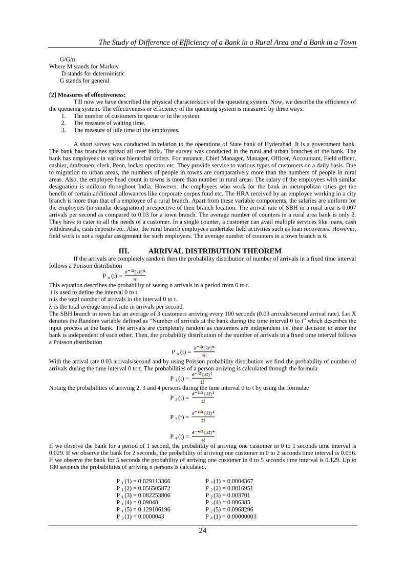
Table - I gives statistics of probabilities of arrivals of 1 person in time interval 0 to t to the rural branch.
Table – I
TIME P 1 (t) TIME P 1 (t)
1 0.029113366 95 0.16485631
2 0.056505872 100 0.149361
3 0.082253806 105 0.134984
4 0.09048 110 0.121714
5 0.129106196 115 0.109522
10 0.222245466 120 0.098365
15 0.286932668 125 0.08819
20 0.329286981 130 0.078943
25 0.354274194 135 0.07056
30 0.365912693 140 0.06298
31 0.36693495 145 0.0561446
32 0.36757717 150 0.049990
33 0.367860924 155 0.039502
34 0.367806839 160 0.039502
35 0.367434636 165 0.035062
40 0.361433054 170 0.0310093
45 0.349974351 175 0.027549
50 0.3346 180 0.024389
55 0.316882349
60 0.297537998
65 0.2774344
70 0.257145
75 0.2371275
80 0.216264
85 0.199104
90 0.18145488
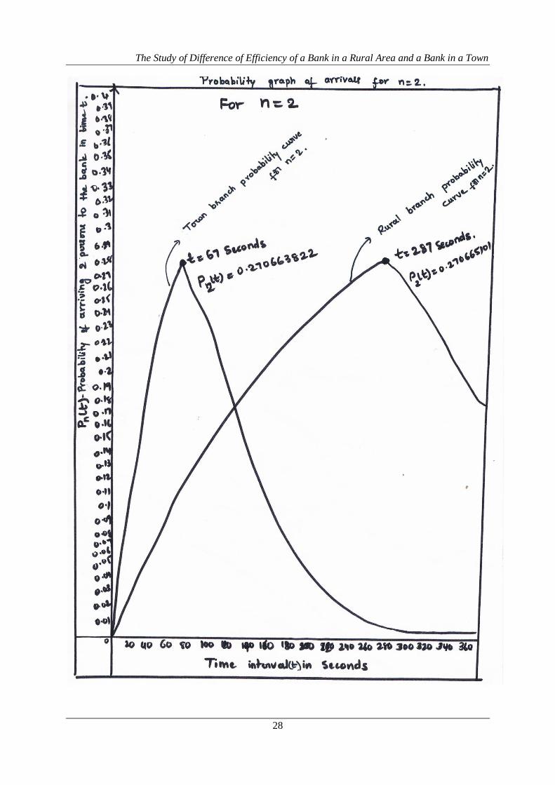
[1] At t = 33 seconds the probability of one person arriving in to the bank is high. Let us denote this time as .
That is is the time where we get the highest probability or crest point for n = 1. Then, by using the formula t = n () + 1 or
n () + 2, n is an integer and n ≥ 2, we can find the time at which we get the highest probability for n = 2, 3, 4, etc. So, we
get the highest probability at time t = 67 seconds for n = 2. We get the highest probability at t = 100 seconds for n = 3. And
for n = 4, we get the highest probability at t = 133 seconds. And so on.
The SBH branch in rural area has an average of 7 customers arriving every 1000 seconds (0.007 arrivals/second
arrival rate). Let X denotes the Random variable defined as “Number of arrivals at the bank during the time interval 0 to t”
which describes the input process at the bank. The arrivals are completely random as customers are independent i.e. their
decision to enter the bank is independent of each other. Then the probability distribution of number of arrivals in a fixed time
interval follows a Poisson distribution
P n (t) =
With the arrival rate 0.007 arrivals/second and by using Poisson probability distribution we find the probability of number of
arrivals during the time interval 0 to t. The probability of one person arriving is calculated through the formula
P 1 (t) =
Noting the probabilities of 2, 3 and 4 persons arriving during the time interval 0 to t by using the formulae
P 2 (t) =
P 3 (t) =
P 4 (t) =
If we observe the bank for a period of 5 seconds, the probability of arriving one customer in 0 to 5 seconds time
interval is 0.033. If we observe the bank for 10 seconds, the probability of arriving one customer in 0 to 10 seconds time
interval is 0.065. If we observe the bank for 15 seconds the probability of arriving one customer in 0 to 15 seconds time
interval is 0.094. Up to 145 seconds the probabilities of arriving n persons is calculated.
The Study of Difference of Efficiency of a Bank in a Rural Area and a Bank in a Town
26
P 1 (5) = 0.029113366
P 1 (10) = 0.056505872
P 1 (15) = 0.082253806
P 1 (20) = 0.09048
P 1 (25) = 0.129106196
Remaining values are tabulated.
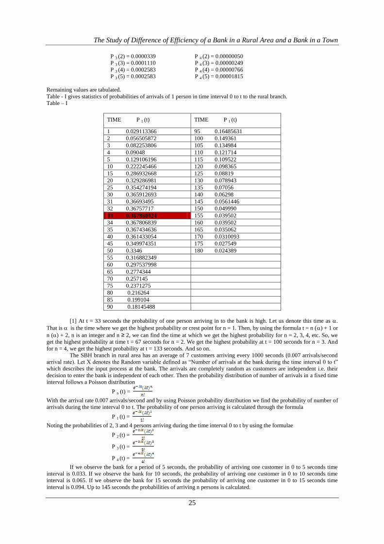
Table - II gives statistics of probabilities of arrivals of 1 person in time interval 0 to t to the rural branch.
Table- II
TIME P 1 (t) TIME P 1 (t)
5 0.033796189 75 0.310566566
10 0.065267567 80 0.319877075
15 0.094534074 85 0.328178726
20 0.121710153 90 0.335532834
25 0.146904978 95 0.341991895
30 0.170222691 100 0.347609712
35 0.191762611 110 0.356520062
40 0.211619447 120 0.362636839
45 0.229883495 140 0.367804876
50 0.246640831 141 0.367848084
55 0.261973494 142 0.367872792
60 0.275959664 143 0.367879256
65 0.288673825 144 0.367867731
70 0.300186933 145 0.367838466
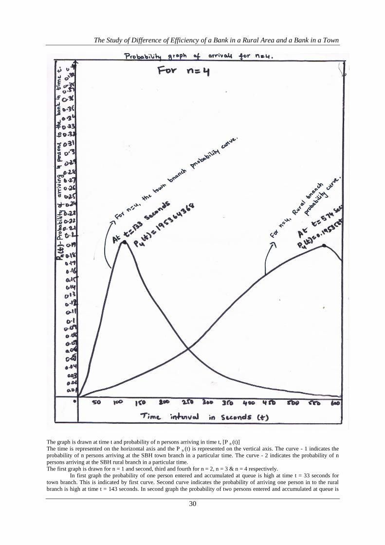
[1] At t = 143 seconds the probability of one person arriving in to the bank is high. Let us denote this time as .
That is is the time where we get the highest probability or crest point for n = 1. Then, by using the formula t = n () + 1 or
n () + 2, n is an integer and n ≥ 2, we can find time at which we get highest probability for n = 2, 3, 4, etc. So we get
highest probability at time t = 287 seconds for n = 2. We get the highest probability at t = 430 seconds for n = 3. And for n =
4, we get highest probability at t = 573 seconds. And so on.
Definition- state dependent service: The situation in which service depends on the number of customers waiting
is referred to as state dependent service.
The Study of Difference of Efficiency of a Bank in a Rural Area and a Bank in a Town
27
Arrival Graphs
The Study of Difference of Efficiency of a Bank in a Rural Area and a Bank in a Town
28

The Study of Difference of Efficiency of a Bank in a Rural Area and a Bank in a Town
29
The Study of Difference of Efficiency of a Bank in a Rural Area and a Bank in a Town
30
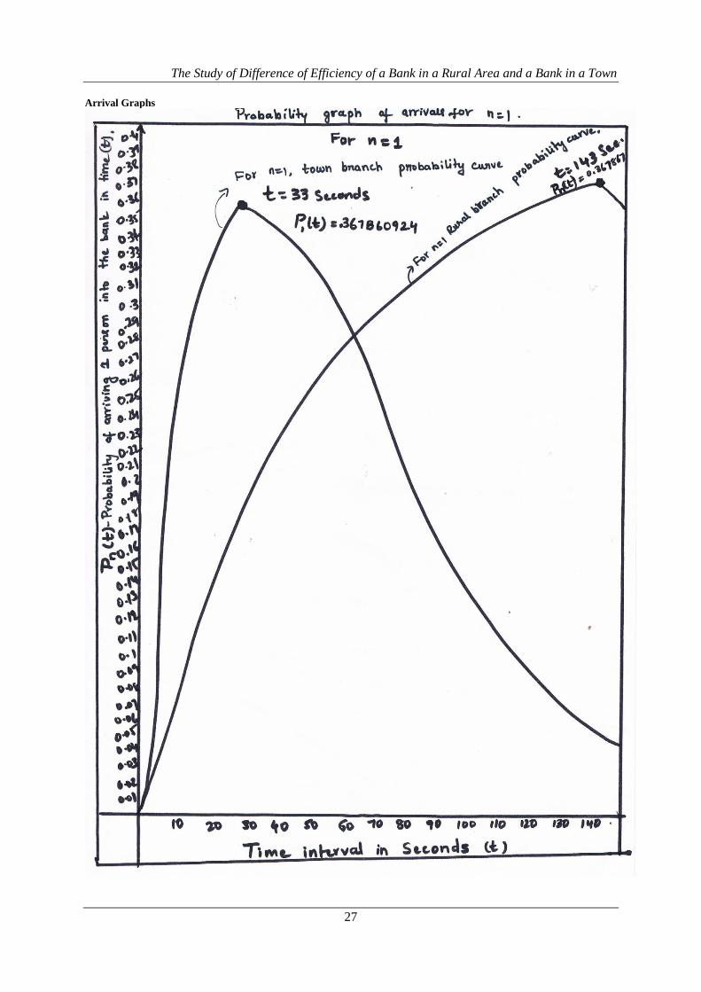
The graph is drawn at time t and probability of n persons arriving in time t, [P n (t)]
The time is represented on the horizontal axis and the P n (t) is represented on the vertical axis. The curve - 1 indicates the
probability of n persons arriving at the SBH town branch in a particular time. The curve - 2 indicates the probability of n
persons arriving at the SBH rural branch in a particular time.
The first graph is drawn for n = 1 and second, third and fourth for n = 2, n = 3 & n = 4 respectively.
In first graph the probability of one person entered and accumulated at queue is high at time t = 33 seconds for
town branch. This is indicated by first curve. Second curve indicates the probability of arriving one person in to the rural
branch is high at time t = 143 seconds. In second graph the probability of two persons entered and accumulated at queue is
The Study of Difference of Efficiency of a Bank in a Rural Area and a Bank in a Town
31
high at time t = 67 seconds for town branch. This is indicated by first curve. Second curve indicates the probability of
arriving two persons in to the rural branch is high at time t = 287 seconds. In third graph probability of three persons entered
and accumulated at queue is high at time 100 seconds for town branch. This is indicated by first curve. Second curve
indicates the probability of arriving three persons in to the rural branch is high at time t = 430 seconds. In fourth graph
probability of four persons entered and accumulated at queue is high at time t = 133 seconds for town branch. This is
indicated by first curve. Second curve indicates the probability of arriving four persons in to the rural branch is high at time t
= 573 seconds. At same time t, the probability of n persons entering the bank is more in a town branch as compared to a
village branch. As the arrival rate is very high in town banks, the number of customers accumulated in the queue is greater.
Since the number of persons accumulated at the queue is one of the way of measurement the efficiency of the queueing
system, we can reason out the efficiency of the branch of the bank in town is less as crowed accumulated is not balanced to
the number of servers when same is measured for the rural area branch. As a result of this, since the service is state
dependent the employees may work fast by observing the long queue or on the contrary may get frustrated and become less
efficient. In the first case the number of customers being served is more. As a result, the employees in town branches are
busy with negligible idle time. In second case the customer gets irate due to the long waiting time. We can also point out this
by taking the alternative measurement of efficiency, the measure of waiting time in the queue or waiting time in the system.
[2] If we study the queueing systems like museums or banks, we consider the waiting time in queue which makes
customer unhappy unlike the study of repairing machines in which we consider waiting time in queue as well as service
time. Considering the random variable T q defined as “Time spent waiting in the queue”. Then the probability distribution of
waiting time is denoted by W q (t), and defined as
W q (t) = 1-
Where is the average amount of work coming to each employee per unit time.
µ is the service rate of the bank.
W q (t) is the probability of a customer waiting for a period of time less than or equal to t for service.
The service rate at the rural and town branches of SBH is equal. i.e 0.032 customers per second.
The arrival rate at the rural and town branches are 0.007 customers per second and 0.03 customers per second respectively.
1 = 0.007 customers/sec.
2 = 0.03 customers/sec.
µ = 0.032 customers/sec.
The amount of work arriving to system per unit time is γ = .
The amount of work arriving to system per unit time is γ = dividing by number of employees c gives average amount of
work coming to each employee per unit time. It is denoted by .
= =
γ = = 0.21875 for a rural branch, γ = = 0.9375 for a town branch.
For the bank in rural area = = 0.109375
For the bank in town area = = 0.15625
Consider W q (t), the probability of a customer waiting for a period of time less than or equal to t for service.
W q (t) = 1-
Here we can find the probability of customer getting serviced in a particular time t.
Graph and Table
For Rural Branch
TIME t W q (t)
5 0.90
10 0.91
15 0.92
20 0.93
25 0.94
30 0.95

The Study of Difference of Efficiency of a Bank in a Rural Area and a Bank in a Town
32
For Town Branch
TIME t W q (t)
5 0.86
10 0.88
15 0.89
20 0.90
25 0.92
30 0.93
The Graph of Waiting Time Distribution:

The Study of Difference of Efficiency of a Bank in a Rural Area and a Bank in a Town
33
The above graph presents an insight in to the probability of getting the service to a customer in a particular time t.
The upper curve represents the probability that an arriving customer has to wait more than time t seconds of the rural branch
for his service. The lower curve represents the probability that an arriving customer has to wait more than time t seconds of
the town branch for his service. From the statistics and the graph we can observe that the probability of the customer waiting
time 5 sec. to get his turn in a village branch is 90 whereby the probability of the customer waiting time 5 sec to go into
service in a town branch is 86 only. Also the probability of the customer waiting time 15 sec. to get his turn in a village
branch is 92 whereby the probability of the customer waiting time 15 sec to go into service in a town branch is 89. By taking
these probability values, we come to the point that the customer of village branch takes less time to complete his work as
compared to the customer in a town branch.
Then we turn our attention to the probability of the system being idle, which is more for rural branch as compared
to the town branch as more value for town branch.
The salary of the employees with similar designation is uniform throughout India. However, the employees who
work for the bank in metropolitan cities get the benefit of certain additional allowances like corporate corpus fund etc. The
HRA received by an employee working in a city branch is more than that of a employee of a rural branch. Apart from these
variable components, the salaries are uniform for the employees (in similar designation) irrespective of their branch location.
Although the employee salary in identical designation is uniform, the quantum of work which they have to do is not equal
and may vary from branch to branch. Various graphs and data from the bank authenticate the same.
The average employee retirement count per year is approximately 600-700. However, recruitments are not in the same
proportion. Numbers of recruitments are only 25 percent of the number of retirements. This leads to additional burden on the
employees of the bank. Though the system is computerized every where the customer has to wait to get his service from the
employees. Like foreign banks, the bank is not sending every day transaction sheet to the customers. This is all due to the
staff problem. The recruitment of staff is through the Banking service recruitment board (BSRB). This should be done by the
Ministry of Finance. And from the data collected from the management of the bank all branches of SBH are getting 100
percent profits every year. The Ministry of Finance should take all these points and need to recruit staff more to give more
customer satisfaction and also the salaries of the employs should effect with arrival rate of the bank as the quantum of work
executed by an employee in a town branch is greater than that of an employee in a rural branch.
IV. CONCLUSION From all of these measures of effectiveness, we come to the inference that the efficiency of a rural branch is higher
than that of a town branch. The rationale behind this conclusion is based on the fact that the number of customers awaiting
service in the queue in a town branch is much higher as compared to that of a rural branch. Secondly, due to the lesser
volume in the queue in a rural branch, the probability of a customer completing his transaction is higher as compared to a
town branch. And an employee in a rural branch is prone to idle time.
As a result, the efficiency in a rural branch is greater than that of a town branch. The need is to improve the
efficiency of a town branch to the levels of a village branch. This can be achieved by increasing the number of employees in
a town branch. Consequently, the busy time per employee can be reduced and thereby increasing efficiency. This in turn will
lead to enhanced customer satisfaction.
REFERENCES [1]. The effect of probabilities of arrivals with time in a bank. By Kasturi Nirmala and Dr.shahnaz Bathul; volume 3,
issue 8, August 2012, International Journal of Science and Engineering Research.
[2]. Fundamentals of Queueing theory by James M Thomson, Donald Gross; Wiley series.
[3]. Operations research by Hamdy Taha.
[4]. An application of Queueing theory to the relationship between Insulin Level and Number of Insulin Receptors by
Cagin Kandemin-Cavas and Levent Cavas.Turkish Journal of Bio Chemistry-2007; 32(1); 32-38
[5]. Queueing theory and its applications; A personal view by Janus Sztrik. Proceedings of the 8th International
conference on Applied Informatics, Eger, Hungary, Jan 27-30, 2010, Vol.1, PP.9-30.
[6]. Case study for Restaurant Queueing model by Mathias, Erwin.2011 International conference on management and
Artificial Intelligence. IPDER Vol.6 (2011) © (2011) IACSIT Press, Bali Indonasia.
[7]. A survey of Queueing theory Applications in Healthcare by Samue Fomundam, Jeffrey Herrmann. ISR Technical
Report 2007-24.
[8]. Graphical Spreadsheet, Simulation of Queues Armann Ingolfsson School of Business, University of Alberta,
Edmonton, Alberta T6G 2R6, Canada, Armann. [email protected] A. Grossman, Jr. Faculty of
Management, University of Calgary, 2500 University Dr. NW Calgary, Alberta, Canada T2N
[9]. The Queueing theory of the Erlang Distributed Inter arrival and Service time by Noln Plumchitchom and Nick T
Thomopoulos. Journal of Research in Engineering and technology; Vol-3, No-4, October-December 2006.