the submanifold geometries associated to grassmannian systems
TRANSCRIPT

1
The Submanifold Geometries associated to Grassmannian Systems
Martina Bruck, Xi Du, Joonsang Park, and Chuu-Lian Terng∗
Abstract
There is a hierarchy of commuting soliton equations associated to each symmetricspace U/K. When U/K has rank n, the first n flows in the hierarchy give rise to a naturalfirst order non-linear system of partial differential equations in n variables, the so calledU/K-system. Let Gm,n denote the Grassmannian of n-dimensional linear subspaces inRm+n, and G1
m,n the Grassmannian of space-like m-dimensional linear subspaces in theLorentzian space Rm+n,1. In this paper, we use techniques from soliton theory to studysubmanifolds in space forms whose Gauss-Codazzi equations are gauge equivalent to theGm,n-system or the G1
m,n-system. These include submanifolds with constant sectionalcurvatures, isothermic surfaces, and submanifolds admitting principal curvature coordi-nates. The dressing actions of simple elements on the space of solutions of the Gm,n
and G1m,n systems correspond to Backlund, Darboux and Ribaucour transformations for
submanifolds.
Table of Contents
1. Introduction . . . . . . . . . . . . . . . . . . . . . . . . . 22. The U/K-system . . . . . . . . . . . . . . . . . . . . . . . 83. Gm,n-systems . . . . . . . . . . . . . . . . . . . . . . . . . 134. G1
m,n-systems . . . . . . . . . . . . . . . . . . . . . . . . . 205. The moving frame method for submanifolds . . . . . . . . . . . . 236. Submanifolds associated to Gm,n-systems . . . . . . . . . . . . . 277. Submanifolds associated to G1
m,n-systems . . . . . . . . . . . . . 378. G1
m,1-system and isothermic surfaces . . . . . . . . . . . . . . . 429. Loop group action for Gm,n-systems . . . . . . . . . . . . . . . 5010. Ribaucour transformations for Gm,n-systems . . . . . . . . . . . 5911. Loop group action for G1
m,n-systems . . . . . . . . . . . . . . 6912. Ribaucour transformations for G1
m,n-systems . . . . . . . . . . . 7313. Darboux transformations for G1
m,1-systems . . . . . . . . . . . . 7514. Backlund transformations . . . . . . . . . . . . . . . . . . . 8015. Permutability formula for Ribaucour transformations . . . . . . . 8816. The U/K-hierarchy and finite type solutions . . . . . . . . . . . 91
∗ Research supported in part by NSF Grant DMS 9626130

2
1. Introduction
Some of the high points in classical differential geometry are the study ofsurfaces in R3 with special geometric properties, to find good coordinates sothat the corresponding Gauss-Codazzi equations have specially nice forms, andto construct explicit examples and deformations of these surfaces. Surfaces withnegative constant Gaussian curvature, surfaces with constant mean curvature,and isothermic surfaces are some of the well-known examples. The Gauss andCodazzi equations of these surfaces are now known to be “soliton” equations.In recent years, modern geometers have found that these equations admit “Laxpairs”, i.e., they can be written as the condition of a family of connections to beflat. The existence of a Lax pair is one of the characteristic properties of solitonequations, and it often gives rise to an action of an infinite dimensional groupon the space of solutions (the dressing action). The geometric transformationsfound for these surfaces by classical geometers such as Backlund, Darboux, andRibaucour transformations, often arise as the dressing action of some simplerational elements. For more detail see [Bo2], [Bo3], [TU3]. In this approach,we start with a class of surfaces in R3. If there are methods to construct aninfinite parameter family of solutions from a given one, then it hints that we maybe able to find a good coordinate system and a Lax pair. Geometers have usedthis method to construct soliton equations involving n variables (cf. [TT], [Te1],[FP2]). But there is no uniform algorithm to achieve this or determine whethera geometric equation for a certain class of submanifolds is a soliton equation.
It is also known that we can associate to each symmetric space U/K a hi-erarchy of soliton equations (cf. [TU1]). For example, the SU(2)-hierarchy isthe hierarchy for the non-linear Schrodinger equation and the SU(2)/SO(2)-hierarchy is the hierarchy for the modified KdV equation. If the rank of thesymmetric space U/K is n, Terng [Te2] put the n first flows together to con-struct a natural non-linear first order system, the U/K-system, and initiated theproject of identifying the submanifold geometry associated to these systems. Thismeans to find submanifolds in certain symmetric space M whose Gauss-Codazziequation is given by the U/K-system and to find the geometric transformationscorresponding to the dressing actions of certain simple elements. This directapproach may provide ways to find Lax pairs for some known class of subman-ifolds, and also may give new interesting class of submanifolds. The main goalof this paper is to carry out this project for the real Grassmannian manifolds ofspace-like m-dimensional linear subspaces in Rm+n and in Rm+n,1.
Below we give a short review of some known facts and outline our results.
• The U/K-systemLet U be a semi-simple Lie group, σ an involution on G, and K the fixed
point set of σ. Then U/K is a symmetric space. The Lie algebra K is the+1 eigenspace of the differential σ∗ of σ at the identity. Let P denote the −1eigenspace of σ∗. Then U = K ⊕ P and
[K,K] ⊂ K, [K,P] ⊂ P, [P,P] ⊂ P.

3
Let A be a maximal abelian subalgebra in P , a1, . . . , an a basis for A, and A⊥the orthogonal complement of A in U with respect to the Killing form <, >.We recall that n = dim(A) is called the rank of the symmetric space. The n-dimensional system associated to U/K, defined by Terng in [Te2], is the followingfirst order non-linear partial differential equation for v : Rn → P ∩A⊥:
[ai, vxj] − [aj , vxi
] =[[ai, v], [aj , v]
], 1 ≤ i = j ≤ n, (1.1)
where vxi= ∂v
∂xi. We will call such system the U/K-system.
• The Lax connectionRecall that a G-valued connection ∂
∂xi+ Ai is flat if its curvature is zero,
i.e., [∂
∂xi+ Ai,
∂
∂xj+ Aj
]= 0
for all i, j. Let V be a linear subspace of a Lie algebra G. A partial differentialequation (PDE) for v : Rn → V admits a Lax connection if there exists a familyof G-valued connection
∂
∂xi+ Ai(v, dv, d2v, · · · , dkv, λ)
such that the PDE for v is given by the flatness of these connections for all λ insome open domain in C. Equation (1.1) admits a Lax connection, ∂
∂xi+ aiλ +
[ai, v]. In other words, v is a solution of (1.1) if and only if[∂
∂xi+ aiλ + [ai, v],
∂
∂xj+ ajλ + [aj , v]
]= 0 (1.2)
for all i, j and λ ∈ C. When n = 2, a Lax connection gives rise to a pair ofcommuting operators. This was first observed by Lax for the KdV equation andis called a Lax pair in the soliton literature.
Note that the connection ∂∂xi
+Ai is flat if and only if the connection 1-formω =
∑i Aidxi is flat, i.e., dω = −ω ∧ ω. In particular, v is a solution of the
U/K-system (1.1) if and only if
θλ =n∑
i=1
(aiλ + [ai, v])dxi (1.3)
is flat for all λ ∈ C. We will also call θλ the Lax connection of the U/K-system.
• Dressing actionThe existence of a Lax connection for an equation often gives rise to an
action of certain subgroup of germs of holomorphic maps at a suitable point on

4
the space of local solutions of the equation. This is called “dressing action” inthe soliton literature. Below we give a rough sketch of the construction of thedressing action (cf. [ZS], [Ch], [TU2]).
If v is a solution of (1.1), then its Lax connection θλ is flat for all λ ∈ C, sothere exists a UC -valued map E(x, λ) such that
E−1dE = θλ, E(0, λ) = I. (1.4)
Since θλ is holomorphic for λ ∈ C, so is E(x, λ). Now let g(λ) be a holomorphicmap defined from a neighborhood of λ = ∞ in S2 = C∪∞ to UC that satisfiescertain U/K-reality condition (defined later) and g(∞) = I. It follows fromthe classical Birkhoff factorization theorem (cf. [PS]) that there exist uniquelyE(x, λ) and g(x, λ) so that
g(λ)E(x, λ) = E(x, λ)g(x, λ), (1.5)
E(x, λ) is holomorphic for λ ∈ C, g(x, λ) is holomorphic near λ = ∞ andg(x,∞) = I. Calculate the residue at λ = ∞ to conclude that
E−1dE =n∑
i=1
(aiλ + [ai, v])dxi
for some v. So v is a new solution of (1.1). The solution v can also be obtainedfrom g as follows: Expand
g(x, λ) = I + m1(x)λ−1 + m2(x)λ−2 + · · ·
at λ = ∞. Thenv = v − p0(m1),
where p0 is the projection onto A⊥ ∩ P . The map
g"v = v
defines the dressing action of the group of germs of holomorphic maps on thespace of local solutions of the U/K-system.
If g(λ) is a meromorphic map on S2 with g(∞) = I, then the factorization(1.5) can be done explicitly by calculating the residues at poles of g(λ). Notethat system (1.1) has a trivial solution v = 0 and
E(x, λ) = exp
(n∑
i=1
aixiλ
)
is the solution of the corresponding linear system (1.4). Therefore g"0 can becomputed explicitly. These explicit solutions correspond to the “pure solitons”in the theory of soliton equations.

5
If g(λ) is a holomorphic map defined in a neighborhood of ∞ in S2 suchthat g(λ)a1g(λ)−1 is a polynomial in λ−1, then the solution g"0 can be obtainedby solving a system of ordinary differential equations on a finite dimensionallinear space. These solutions are the so called “finite type solutions”. Finitetype solutions have been used successfully to construct constant mean curvaturetori in R3(c) by Pinkall and Sterling in [PiS], in 3-dimensional space forms byBobenko in [Bo1], and harmonic maps from a torus to a symmetric space byBurstall, Ferus, Pedit and Pinkall in [BFPP].
• Cauchy problemIf a1 is regular, then the linear map ad(a1) : P ∩ A⊥ → K is injective.
It follows from Cartan-Kahler Theorem that if v0 : (−δ, δ) → P ∩ A⊥ isreal analytic, then system (1.1) has a unique local analytic solution such thatv(x1, 0, · · · , 0) = v0(x1). If the initial data v0 is not real analytic but is rapidlydecaying, then we can use the inverse scattering method developed by Beals andCoifman [BC] to solve the initial value problem (cf. [TU1], [Te2]).
• Gauge equivalent systemsLet θλ be the flat connection (1.3) associated to the solution v of the U/K-
system (1.1), and g : Rn → UC a smooth map. Then the gauge transformation
g ∗ θλ = gθλg−1 − dgg−1
is again a flat connection 1-form for all λ ∈ C. However, the differential equationgiven by the condition that g ∗ θλ is flat for all λ has a different form. We saythis new equation is gauge equivalent to system (1.1). For example:(i) Since θλ satisfies the U/K-reality condition, θ0 is a K-valued flat connection
1-form. Hence there exists g such that g−1dg = θ0. A direct computationshows that the gauge transformation of θλ by g is
g ∗ θλ = gθλg−1 − dgg−1 =n∑
i=1
gaig−1λdxi.
Write Ai = gaig−1. The equation given by the flatness of g∗θλ is the curved
flat system studied by Ferus and Pedit in [FP1].(ii) Suppose K = K1 × K2. Let v be a solution of the U/K-system, and
g−1dg = θ0. Since θ0 ∈ K, g(x) ∈ K = K1 × K2. So we can writeg = (g1, g2) ∈ K1 × K2. A direct computation shows that the coefficientsof λ0 in g1 ∗ θλ and g2 ∗ θλ are in K2 and K1 respectively. The equationsgiven by the flatness of g1 ∗ θλ and g2 ∗ θλ are called the U/K-system I andII respectively.
• Gauss-Codazzi equations for Submanifolds in space formsLet O(n, 1) denote the group of all g ∈ GL(n+1) that preserves the bilinear
formx2
1 + · · · + x2n − x2
n+1.

6
Henceforth in this paper, we use the following notations:
Gm,n = O(m + n)/O(m) × O(n), G1m,n = O(m + n, 1)/O(m) × O(n, 1).
Let Nn(c) denote the n-dimensional space form with curvature c, i.e., thecomplete, simply connected Riemannian manifold with constant sectional curva-ture c. So Nn(c) is Rn, Sn and Hn for c = 0, 1,−1 respectively. The Levi-Civitaconnection 1-form of Nn(c) can be read from the flatness of a so(n), so(n + 1)and o(n, 1)- valued connection 1-form. The Gauss-Codazzi equation of a sub-manifold in Nn(c) is given by the flatness of the restriction of this connection1-form to the submanifold. The Fundamental Theorem of Submanifolds statesthat each solution of the Gauss-Codazzi equation correspond to a submanifoldin Nn(c), unique up to ambient isometry. So if v is a solution of the Gm,n- orG1
m,n-system I or II, then the corresponding Lax connection θλ at λ = 1 gives riseto a submanifold of a certain space form. Using the method of moving frames,special properties of the flat connection θ1 can be translated easily to geometricproperties of the corresponding submanifolds.
• Submanifolds corresponding to the Gm,n- and G1m,n-system I
In [Te2], Terng proved that solutions of the Gn,n-, Gn,n+1- and G1n,n-system
I correspond to local isometric immersions of the space form Nn(c) in N2n(c)with flat normal bundle for c = 0, 1, and −1 respectively. We generalize thisresult to the Gm,n- and G1
m,n-system I for any m ≥ n. They give rise to localisometric immersions of Nn(c) into Nn+m(c).
• Submanifolds corresponding to Gm,n- and G1m,n-system II
In order to explain the submanifold geometry corresponding to the Gm,n-and G1
m,n-system II, we first need to review some classical surface theory. LetM be a surface in R3 with curvature K = −1, and e3 its unit normal field.Then there exists a line of curvature coordinate system (x, y) such that the twofundamental forms of M are
I1 = cos2 u dx2 + sin2 u dy2, II1 = sinu cos u (dx2 − dy2).
Since the unit sphere is totally umbilic, the fundamental forms for S2 in (x, y)coordinates via the parametrization e3(x, y) are
I2 = sin2 u dx2 + cos2 u dy2, II2 = −(sin2 u dx2 + cos2 u dy2).
The Gauss-Codazzi equations for M (curvature −1) and e3 (curvature 1) are thesame sine-Gordon equation
uxx − uyy = sinu cos u, (SGE)
and the tangent plane of M at (x, y) is the same as the tangent plane of the sphereat e3(x, y). A direct computation shows that such u gives rise to a solution of

7
the G3,2-system II. This is a special case. In fact, we show that each solution ofthe G3,2-system II corresponds to a pair of surfaces (X1, X2) in R3 with commonline of curvature coordinates x, y such that the tangent plane at X1(x, y) is equalto the tangent plane at X2(x, y) and their fundamental forms are
I1 = cos2 u dx2 + sin2 u dy2, II1 = g1 cos u dx2 + g2 sinu dy2,
I2 = sin2 u dx2 + cos2 u dy2, II2 = −g1 sinu dx2 + g2 cos u dy2
for some functions u, g1, g2. Moreover, the Gaussian curvature
K1(x, y) = −K2(x, y).
For general m > n, we prove that each solution of the Gm,n-system II (G1m,n−1-
system II respectively) gives rise to an n-tuple of n-dimensional submanifolds(X1, · · · , Xn) in Rm with flat normal bundles and common line of curvaturecoordinates (x1, · · · , xn) such that fundamental forms of Xj are
Ij =n∑
i=1
a2ji(x)dx2
i , IIj =n,m−n∑i=1,k=1
ajigki dx2i en+k
for some (aij(x)) ∈ O(n) (∈ O(n − 1, 1) respectively) and gki(x).If we use another standard form of O(n + 1, 1), the group of g ∈ GL(n + 2)
that leaves the bi-linear from
x21 + · · · + x2
n + 2xn+1xn+2
invariant, then the corresponding 2-tuple (X1, X2) in Rn for the G1n,1-system II
has the property that X1 is an isothermic surface and X2 is a Christoffel dual ofX1. This was proved by Burstall, Hertrich-Jeromin, Pedit and Pinkall in [BHPP]for n = 2 and by Burstall in [Bu] for general n.
• Backlund transformations and dressing actionLet M, M∗ be two surfaces in R3. A diffeomorphism . : M → M∗ is called
a Backlund transformation with constant θ if for all p ∈ M ,(a) pp∗ is tangent to both M and M∗ at p and p∗ = .(p),(b) d(p, p∗) = sin θ,(c) the angle between TMp and TM∗p∗ is θ.Backlund proved ([Ba]) that if . is a Backlund transformation, then both Mand M∗ have curvature −1. Moreover, if M is a surface in R3 with K = −1,0 < θ < π a constant, and v0 ∈ TMp0 a unit vector that is not a principaldirection, then there exist a unique surface M∗ and a Backlund transformation. : M → M∗ such that .(p0) = p0 +sin θ v0. Analytically, this gives a method ofconstructing new solution of SGE from a given one. Backlund transformations

8
have been generalized to isometric immersions of Nn(c) in N2n−1(c+1) by Terngand Tenenblat for c = −1 in [TT] and by Tenenblat for c = 0, 1 in [Ten].
Terng and Uhlenbeck proved in [TU2] that the dressing action of a mero-morphic map with one pole on the space of solutions of SGE gives rise exactlyto the classical Backlund transformations. We generalize this result to Gn,n andG1
n,n-systems.
• Ribaucour transformations and dressing actionLet M, M be two surfaces in R3. A diffeomorphism . : M → M is called a
Ribaucour transformation if for all p ∈ M(a) TMp = TM(p),(b) the normal line at p to M meets the normal line at .(p) to M at equidistance
r(p),(c) the line through p in the principal direction e of M meets the line through
.(p) in the direction .∗(e) at a point at equidistance s(p).The notion of Ribaucour transformations has a natural generalization to subman-ifolds in space forms with flat normal bundle ([DT]). We show that the dressingaction of rational maps with two simple poles on the solutions of the Gm,n- andG1
m,n-system I and II correspond to Ribaucour transformations for submanifolds.
• Organization of the paperWe review some general facts about the U/K-system in section 2, write down
the Gm,n-systems explicitly in section 3, and the G1m,n-systems in section 4. We
review the method of moving frames in section 5. We describe submanifolds asso-ciated to various Gm,n-systems and G1
m,n-systems in section 6 and 7 respectively.In section 8, we study relations between constant mean curvature in 3-dimensionspace forms, isothermic surfaces and G1
m,1-systems. The dressing action of arational map with two simple poles on solutions of the Gm,n- and G1
m,n-systemsare written down explicitly in section 9 and 11 respectively. The correspondinggeometric transformations are given in section 10 and 12. Burstall [Bu] gave ageneralization of isothermic surfaces in R3 and their Darboux transformationsto isothermic surfaces in Rn. In section 13, we show that the dressing action ofa rational map with two poles on the space of solutions of the G1
n,1-system IIgives rise to these Darboux transformations. In section 14, we give a relationbetween the dressing action of loop with one simple pole and Backlund transfor-mations. A permutability formula for Ribaucour transformations is explained insection 15, and relation between dressing action and finite type solutions of theU/K-system are given in the last section.
2. The U/K-System
A connection of a trivial principal U -bundle over Rn is:∂
∂xi+ Ai, 1 ≤ i ≤ n,

9
for some smooth maps Ai : Rn → U . The curvature of this connection is
Ωij =[
∂
∂xi+ Ai,
∂
∂xj+ Aj
]= (Aj)xi
− (Ai)xj+ [Ai, Aj ].
A connection is flat if its curvature is zero.The following Proposition, which is well-known, gives several equivalent con-
ditions for a connection to be flat. The proof follows from a direct computation.
2.1 Proposition. Let A1, · · · , An : Rn → U be smooth maps. The followingstatements are equivalent:
(1) the connection ∂∂xi
+ Ai(x) is flat, i.e., [ ∂∂xi
+ Ai,∂
∂xj+ Aj ] = 0,
(2) (Aj)xi− (Ai)xj
+ [Ai, Aj ] = 0,
(3) the connection 1-form θ =n∑
i=1
Aidxi is flat, i.e., dθ + θ ∧ θ = 0.
(4)
Exi= EAi, 1 ≤ i ≤ n, (2.1)
is solvable for E : Rn → U .
E is called a trivialization of the flat connection θ =∑
i Aidxi if it is a solutionof (2.1) or equivalently if
E−1dE =n∑
i=1
Aidxi.
It follows from a direct computation and Proposition 2.1 that
2.2 Proposition ([Te2]). The following statements are equivalent for a mapv : Rn → P ∩A⊥:
(i) v is a solution of the U/K-system (1.1),
(ii) [∂
∂xi+ λai + [ai, v],
∂
∂xj+ λaj + [aj , v]
]= 0, ∀ λ ∈ C, (2.2)
(iii) θλ is a flat UC = U ⊗ C-connection 1-form on Rn for all λ ∈ C, where
θλ =n∑
i=1
(aiλ + [ai, v])dxi, (2.3)
(iv) there exists E so that E−1dE = θλ.

10
The one parameter family of flat connections (2.2) or (2.3) is called the Laxconnection of the U/K-system (1.1).
An element b ∈ P is called regular if the orbit at b for the Ad(K)-action isa principal orbit. Let A be a maximal abelian subalgebra in P ,
KA = ξ ∈ K | [ξ, a] = 0 ∀ a ∈ A,and K⊥A the orthogonal complement of KA in K. It follows from standard theoryof symmetric space (cf. [H]) that if b ∈ A is regular, then ad(b) maps K⊥A andP ∩ A⊥ isomorphically to P ∩ A⊥ and K⊥A respectively.
2.3 Proposition. Let a1, · · · , an be a basis of a maximal abelian subalgebraA in P , and ui : Rn → K⊥A smooth maps for 1 ≤ i ≤ n. If
θλ =n∑
i=1
(aiλ + ui)dxi (2.4)
is a flat connection 1-form on Rn for all λ ∈ C, then there exists a unique mapv : Rn → P ∩A⊥ such that ui = [ai, v].
PROOF. Choose a basis b1, · · · , bn of A such that each bi is regular. Writebj =
∑i cijai. Make a change of coordinates xi =
∑j cijyj . Then
θλ =∑
i
(aiλ + ui)dxi =∑
j
(bjλ + uj)dyj ,
where uj =∑
i cijui ∈ K ∩A⊥. Note that θλ is flat for all λ if and only if[bi, uj ] = [bj , ui],(uj)xi
− (ui)xj+ [ui, uj ] = 0.
(2.5)
Because b1, · · · , bn are regular, ad(bj) maps P ∩ A⊥ isomorphically to K ∩ A⊥.Hence there exists a unique vj ∈ P∩A⊥ such that uj = ad(bj)(vj) for 1 ≤ j ≤ n.Then the first equation of (2.5) implies that
ad(bi) ad(bj)(vj) = ad(bj) ad(bi)(vi).
Since [bi, bj ] = 0, ad(bi) ad(bj) = ad(bj) ad(bi). But ad(bi) is injective on P∩A⊥implies that vi = vj , which will be denoted by v. We compute directly to get
uj =∑
i
cij ui =∑
i
cij [bi, v]
=∑
i
cij
[∑k
ckiak, v
]= [aj , v],
where (cij) is the inverse of (cij).
The following Proposition is immediate:

11
2.4 Proposition. If θ is a flat G-valued connection 1-form and g : Rn → G asmooth map, then the gauge transformation of θ by g,
g ∗ θ = gθg−1 − dgg−1,
is also flat. Moreover, if E is a trivialization of θ, then Eg−1 is a trivializationof g ∗ θ.
Consider the system of PDE for
(A1, · · · , An, B1, · · · , Bn) : Rn →n∏
i=1
P ×n∏
i=1
K
given by the condition that
n∑i=1
(Aiλ + Bi)dxi
is a flat connection on Rn for all λ ∈ C. Or equivalently,
(Ajλ + Bj)xi − (Aiλ + Bi)xj + [Aiλ + Bi, Ajλ + Bj ] = 0
for all λ ∈ C. By comparing coefficients of λ2, λ and the constant term, we get
[Ai, Aj ] = 0,(Ai)xj
− (Aj)xi= [Ai, Bj ] + [Bi, Aj ],
(Bi)xj − (Bj)xi = [Bi, Bj ].(2.6)
2.5 Proposition. Let Ωλ =∑
i(Aiλ + Bi)dxi, Ai ∈ P and Bi ∈ K. If[Ai, Aj ] = 0 for all 1 ≤ i, j ≤ n, then Ωλ is flat for all λ ∈ C if and only if Ωλ0
is flat for some non-zero real or pure imaginary λ0.
PROOF. If Ωλ0 is flat, then
(λ0Aj + Bj)xi − (λ0Ai + Bi)xj + [λ0Ai + Bi, λ0Aj + Bj ] = 0. (2.7)
So both the K and P components of the left hand side of the equation must bezero. Since U/K is a symmetric space,
[K,K] ⊂ K, [K,P] ⊂ P, [P,P] ⊂ K.
Equate the K and P components of (2.7) to get(Bj)xi − (Bi)xj + [Bi, Bj ] = 0,(Aj)xi
− (Ai)xj+ [Ai, Bj ] + [Bi, Aj ] = 0.
12
But this is the equation for Ωλ to be flat for all λ ∈ C.
Restrict system (2.6) to the case when all Bi = 0 to get a system for maps(A1, · · · , An) : Rn → P × · · · × P:
[Ai, Aj ] = 0,(Ai)xj = (Aj)xi , for all i = j. (2.8)
This is the Curved Flat system associated to U/K defined by Ferus and Pedit in[FP]. Its Lax connection is[
∂
∂xi+ Aiλ,
∂
∂xj+ Ajλ
]= 0, ∀ λ ∈ C.
The second equation of (2.8) implies that∑
i Aidxi is exact. So we get
2.6 Proposition. Let Ai(x) ∈ P . Then∑
i λAi(x)dxi is flat for all λ ∈ C ifand only if [Ai, Aj ] = 0 for all 1 ≤ i, j ≤ n and there exists a map X : Rn → Psuch that
dX =n∑
i=1
Aidxi.
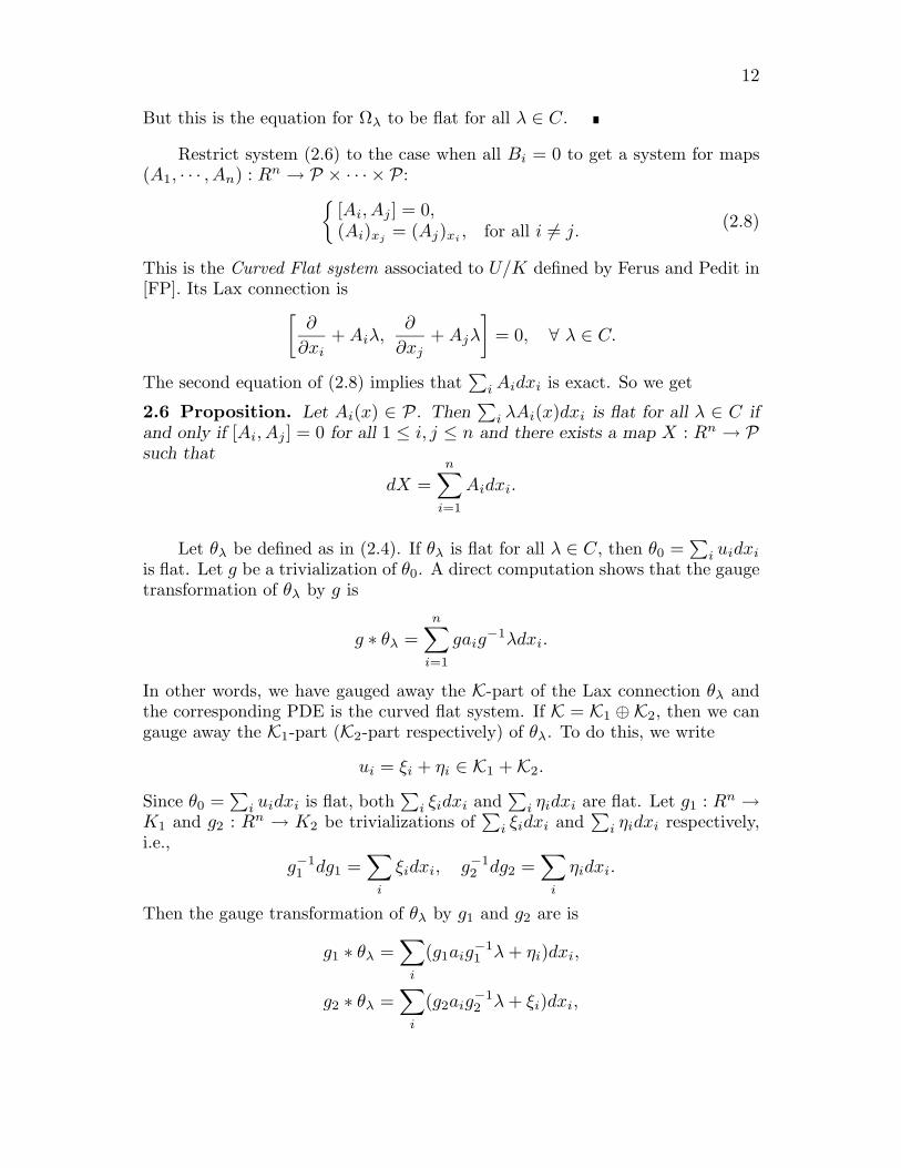
Let θλ be defined as in (2.4). If θλ is flat for all λ ∈ C, then θ0 =∑
i uidxi
is flat. Let g be a trivialization of θ0. A direct computation shows that the gaugetransformation of θλ by g is
g ∗ θλ =n∑
i=1
gaig−1λdxi.
In other words, we have gauged away the K-part of the Lax connection θλ andthe corresponding PDE is the curved flat system. If K = K1 ⊕K2, then we cangauge away the K1-part (K2-part respectively) of θλ. To do this, we write
ui = ξi + ηi ∈ K1 + K2.
Since θ0 =∑
i uidxi is flat, both∑
i ξidxi and∑
i ηidxi are flat. Let g1 : Rn →K1 and g2 : Rn → K2 be trivializations of
∑i ξidxi and
∑i ηidxi respectively,
i.e.,g−11 dg1 =
∑i
ξidxi, g−12 dg2 =
∑i
ηidxi.
Then the gauge transformation of θλ by g1 and g2 are is
g1 ∗ θλ =∑
i
(g1aig−11 λ + ηi)dxi,
g2 ∗ θλ =∑
i
(g2aig−12 λ + ξi)dxi,

13
respectively.The U/(K1 × K2)-system I is the PDE for g1 : Rn → K1 and η1, · · · , ηn :
Rn → K2 ∩ K⊥A such that
θIλ =
∑i
(g1aig−11 λ + ηi)dxi
is flat for all λ ∈ C, i.e.,[g−1
1 (g1)xi , aj ] − [g−11 (g1)xj , ai] + [ai, g
−11 ηjg1] + [g−1
1 ηig1, aj ] = 0,(ηj)xi
− (ηi)xj+ [ηi, ηj ] = 0. (2.9)
Similarly, the U/(K1 × K2)-system II is the PDE for g2 : Rn → K2 andξ1, · · · , ξn : Rn → K1 ∩ K⊥A such that
θIIλ =
∑i
(g2aig−12 λ + ξi)dxi
is flat for all λ ∈ C, i.e.,[g−1
2 (g2)xi, aj ] − [g−1
2 (g2)xj, ai] + [ai, g
−12 ξjg2] + [g−1
2 ξig2, aj ] = 0,(ξj)xi
− (ξi)xj+ [ξi, ξj ] = 0.
(2.10)
3. Gm,n-systems
In this section, we assume
U/K = Gm,n = O(m + n)/(O(m) × O(n)) with m ≥ n.
We write down the Gm,n-systems I and II explicitly.Let U = o(m + n), and σ : U → U be the involution defined by σ(X) =
I−1m,nXIm,n, where
Im,n =(
Im 00 −In
).
Let K and P denote the +1 and −1 eigenspaces of σ respectively. Then U = K+Pis a Cartan decomposition of U/K, where
K = o(m) × o(n) =(
Y1 00 Y2
) ∣∣∣∣ Y1 ∈ o(m), Y2 ∈ o(n)
,
P =(
0 ξ−ξt 0
) ∣∣∣∣ ξ ∈ Mm×n
.

14
Here Mm×n is the set of m × n matrices. Note that
A =(
0 −DDt 0
) ∣∣∣∣ D = (dij) ∈ Mm×n, dij = 0 if i = j
.
is a maximal abelian subalgebra in P and
P ∩ A⊥ =(
0 ξ−ξt 0
) ∣∣∣∣ ξ = (ξij) ∈ Mm×n, ξii = 0 for 1 ≤ i ≤ n
.
Let
ai =(
0 −Di
Dti 0
),
where Di ∈ Mm×n is the matrix all whose entries are zero except the ii-th entryis equal to 1. Then a1, . . . , an form a basis of A. The U/K-system (1.1) for thissymmetric space is the following PDE for ξ = (ξij) : Rn → Mm×n with ξii = 0for all 1 ≤ i ≤ n:
Diξ
txj
− ξxj Dti − Djξ
txi
+ ξxiDtj = [Diξ
t − ξDti , Djξ
t − ξDtj ], i = j,
Dtiξxj
− ξtxj
Di − Dtjξxi
+ ξtxi
Dj = [Dtiξ − ξtDi, D
tjξ − ξtDj ], i = j.
(3.1)
Its Lax connection (2.3) is
θλ =∑
i
λ
(0 −Di
Dti 0
)+
(Diξ
t − ξDti 0
0 −ξtDi + Dtiξ
)dxi. (3.2)
Next we write down the Gm,n-system I and II explicitly. Let
g =(
A 00 B
)∈ O(m) × O(n)
be a solution of
g−1dg = θ0 =n∑
i=1
(Diξ
t − ξDti 0
0 −ξtDi + Dtiξ
)dxi.
Let
g1 =(
A 00 I
), g2 =
(I 00 B
).
Write
ξ =(
FG
), Di =
(Ci
0
), A = (A1, A2),

15
where F, Ci ∈ gl(n), G ∈ M(m−n)×n, A1 ∈ Mm×n, and A2 ∈ Mm×(m−n).Then
g1aig−11 =
(0 −A1Ci
CiAt1 0
).
LetM0
m×n = A1 ∈ Mm×n |At1A1 = I,
gl(n)∗ = (xij) ∈ gl(n) | xii = 0, 1 ≤ i ≤ n.
The U/K-system I is the PDE for (A1, F ) : Rn → M0m×n × gl∗(n) such
that
θIλ =
n∑i=1
(0 −A1Ciλ
CiAt1λ −F tCi + Ct
iF
)dxi (3.3)
is flat for all λ ∈ C, i.e.,
(aij)xk= fjkaik, if k = j,
(fij)xj+ (fji)xi
+∑
k fikfjk = 0, if i = j,(fij)xk
= fikfkj , if i, j, k are distinct,(3.4)
where A = (aij) and F = (fij). Note that equation (3.4) is the condition thatthe above θI
λ is flat for λ = 1. So we have
3.1 Proposition. The following statements are equivalent for map (A1, F ) :Rn → M0
m×n × gl∗(n):(i) (A1, F ) is a solution of the Gm,n-system I (3.4).(ii) θI
λ defined by (3.3) is flat for all λ ∈ C.(iii) θI
λ defined by (3.3) is flat for λ = 1.
Note that if aij = 0 for all 1 ≤ j ≤ n, then the first set of equations of (3.4)implies that F can be computed from the i-th row of A1 by fjk = (aij)xk
/aik.
Next we explain the reality conditions. Recall that a symmetric space U/Kis determined by a conjugate linear Lie algebra involution τ and a complex linearLie algebra involution σ on the complexified Lie algebra UC = U ⊗ C such that(i) τ and σ commute,(ii) U is the fixed point set of τ , and K and P are the +1,−1 eigenspaces of σ
on U respectively, and U = K + P is the Cartan decomposition.We still use τ and σ to denote the corresponding involutions on the group UC .
A map g : C → UC (g : C → UC respectively) is said to satisfy the U/K-reality condition if
τ(g(λ)) = g(λ), σ(g(−λ)) = g(λ). (3.5)
A direct computation gives

16
3.2 Proposition.(i) If A(λ) =
∑i Aiλ
i : C → UC satisfies the U/K-reality condition, thenAi ∈ K if i is even and is in P if i is odd.
(ii) The Lax pair θλ defined by (2.3) for the U/K-system (1.1) satisfies theU/K-reality condition.
3.3 Definition. A frame for a solution v of the U/K-system (I, II respec-tively) is a trivialization of the corresponding Lax connection θλ (θI
λ, θIIλ respec-
tively) that satisfies the U/K-reality condition.
3.4 Remark.(i) If g : C → UC satisfies the U/K-reality condition, then g(0) ∈ K.(ii) If E(x, λ) is the trivialization of θλ defined by (2.3) such that E(0, λ) satisfies
the U/K-reality condition, then E also satisfies the U/K-reality condition.
Let p ∈ O(m) be a constant matrix. The gauge transform of θIλ by g =(
p 00 I
)is
g ∗ θIλ =
(0 −pA1Ciλ
CtiA
t1p
tλ −F tCi + CtiF
),
which is flat for all λ ∈ C. Note that the coefficient of λ in g ∗ θλ lies in P , theconstant term lies in K, and
(pA1)t(pA1) = At1p
tpA1 = At1A1 = I.
So it follows from Proposition 3.1 that
3.5 Corollary. Let (A1, F ) be a solution of the Gm,n-system I (3.4), and p ∈O(m) a constant matrix. Then (pA1, F ) is also a solution of (3.4). Moreover, ifEI is a frame for (A1, F ), then EIp−1 is a frame for (pA1, F ).
3.6 Proposition.
(i) Suppose ξ =(
FG
)is a solution of the Gm,n-system (3.1), θλ the corre-
sponding Lax connection, and g =(
A 00 B
): Rn → O(m)×O(n) satisfies
g−1dg = θ0. Write A = (A1, A2) with A1 ∈ Mm×n. Then (A1, F ) is asolution of the Gm,n-system I (3.4).
(ii) Conversely, if (A1, F ) is a solution of the Gm,n-system I (3.4), then there
exists an M(m−n)×n-valued map G such that ξ =(
FG
)is a solution of (3.1).
PROOF.(i) follows from the definition of the U/K-system I.

17
(ii) Choose A2 so that A = (A1, A2) ∈ O(m). Let g =(
At 00 I
). Then
the gauge transformation of g on θIλ is
g∗θIλ = gθI
λg−1 − dgg−1
=∑
i
λ
( 0 0 −Ci
0 0 0Ci 0 0
)+
(At
1 (A1)xiAt
1 (A2)xi0
At2 (A1)xi
At2 (A2)xi
00 0 −F tCi + CiF
)dxi.
Although this does not have the same shape as the Lax pair θλ of the Gm,n-system, we show below that it can be gauged to one. From (3.4), we have
dA1 = A1
∑(CiF
t − FCi)dxi + ζ∑
Cidxi (3.6)
for some ζ : Rn → Mm×n. Thus
At2dA1 = At
2ζ∑
Cidxi. (3.7)
Since A−1dA is flat and
A−1dA =(
At1dA1 At
1dA2
At2dA1 At
2dA2
),
we havedAt
2 ∧ dA2 + At2dA1 ∧ At
1dA2 + At2dA2 ∧ At
2dA2 = 0. (3.8)
By (3.7), At1dA2 = (dAt
2A1)t = −(At2dA1)t = −
∑Ciζ
tA2dxi. So it followsfrom (3.8) that At
2dA2 is flat, and hence there exists h : Rn → O(m − n) such
that h−1dh = At2dA2. Thus if we do a gauge transform by h =
(I 0 00 h 00 0 I
)on
g ∗ θIλ, the resulting connection 1-form is
h ∗ (g ∗ θIλ) =
∑ λ
( 0 0 −Ci
0 0 0Ci 0 0
)+
(At
1(A1)xi−Ciζ
tA2ht 0
hAt2ζCi 0 00 0 −F tCi + CiF
)dxi.
SetG = −hAt
2ζ.
From (3.6), we have At1(A1)xi −(CiF
t−FCi) = Y Ci, where Y = At1ζ. Since the
left-hand side is skew-symmetric, so is Y Ci. But Y Ci = −CiY for all 1 ≤ i ≤ n

18
implies that Y = 0. It follows that h ∗ (g ∗ θIλ) is the θλ defined by (3.2) with
ξ =(
FG
). In other words, ξ is a solution of (3.1).
The Gm,n-system II is the PDE for
(F, G, B) : Rn → gl∗(n) ×M(m−n)×n × O(n)
such that
θIIλ =
n∑i=1
(−FCi + CiFt CiG
t −CiBtλ
−GCi 0 0BCiλ 0 0
)dxi (3.9)
is flat for all λ ∈ C, i.e.,
(fij)xi + (fji)xj +∑n
k=1 fkifkj +∑m−n
k=1 gkigkj = 0, if i = j,(fij)xk
= fikfkj , if i, j, k are distinct,(bij)xk
= fkjbik, if j = k,(gij)xk
= fkjgik, if j = k.(3.10)
As a consequence of Proposition 2.5 we get
3.7 Proposition. Given (F, G, B) : Rn → gl∗(n) × M(m−n)×n × O(n), thefollowing statements are equivalent:
(i) (F, G, B) is a solution of the Gm,n-system II (3.10).
(ii) θIIλ defined by (3.9) is flat for all λ ∈ C,
(iii) θIIλ defined by (3.9) is flat for λ = 1.
Note that if E is a frame for v =(
FG
), then E(x, 0) =
(A(x) 0
0 B(x)
)
and EII = E
(A−1 00 In
)is a frame for (F, G, B).
If bji = 0 for all 1 ≤ i ≤ n, then the third equation of (3.10) implies thatfki = (bji)xk
/bjk if k = i. In other words, generically system (3.10) dependsonly on B and G.
3.8 Corollary. If (F, G, B) is a solution of the Gm,n-system II (3.10) and C ∈O(n) a constant matrix, then (F, G, CB) is also a solution of (3.10). Moreover,if EII is a frame for (F, G, B), then EIIC−1 is a frame for (F, G, CB).
Let U/K = Gm,n+1 with m ≥ n + 1. The rank of U/K is n + 1. So thecorresponding U/K-system has (n+1) independent variables. Below we considera partial U/K-system of n-variables. Let (m1, m2, m3, m4) = (n, m − n, n, 1).

19
We partition a matrix A in o(m + n + 1) into 4 × 4 blocks A = (Aij), whereAij ∈ Mmi×mj
. Let
ai =
0 0 −Ci 00 0 0 0Ci 0 0 00 0 0 0
, where Ci = diag(0, . . . , 1, . . . , 0) as before.
Then the space A spanned by a1, · · · , an is an n-dimensional abelian subspace ofP . Let KA and UA denote the centralizer of A in K and U respectively. ThenP ∩ U⊥A is the space of elements of the form
v =
0 0 F b0 0 G 0
−F t −Gt 0 0−bt 0 0 0
,
where, F ∈ gl(n)∗, b ∈ Mn×1, G ∈ M(m−n)×n.The partial Gm,n+1-system is the PDE for (F, G, b) : Rn → gl(n)∗ ×
M(m−n)×n ×Mn×1 such that
Θλ =∑
i
λ
0 0 −Ci 00 0 0 0Ci 0 0 00 0 0 0
dxi
+∑
i
−FCi + CiFt CiG
t 0 0−GCi 0 0 0
0 0 −F tCi + CiF Cib0 0 −btCi 0
dxi
(3.11)
is flat for all λ ∈ C, i.e.,
(fij)xi + (fji)xj +∑
k fkifkj +∑
k gkigkj = 0, if i = j,(fij)xk
= fikfkj , if i, j, k distinct,(gij)xk
= gikfkj , if k = j,(fij)xj + (fji)xi +
∑k fikfjk + bibj = 0, if i = j,
(bi)xj= fijbj .
(3.12)
The partial Gm,n+1-system I is the PDE for maps
(A1, F, b) : Rn → M0m×n × gl∗(n) ×Mn×1
such that
ΘIλ =
∑i
( 0 −A1Ciλ 0CiA
t1λ −F tCi + CiF Cib
0 −btCi 0
)dxi (3.13)

20
is flat for all λ ∈ C, i.e.,
(fij)xj + (fji)xi +∑n
k=1 fikfjk + bibj = 0, i = j,(fij)xk
= fikfkj , i, j, k distinct,(bi)xj
= fijbj , i = j,(aki)xj
= fijakj , i = j.
(3.14)
By Proposition 2.5 we have
3.9 Proposition. Given a map (A1, F, b) : Rn → M0m×n × gl∗(n) × Mn×1,
the following statements are equivalent:(i) (A1, F, b) is a solution of the partial Gm,n+1-system I (3.14),(ii) ΘI
λ defined by (3.13) is flat for all λ ∈ C,(iii) ΘI
λ defined by (3.13) is flat for λ = 1.
4. G1m,n-Systems
In this section, we assume m ≥ n + 1 and
U/K = G1m,n = O(m + n, 1)/(O(m) × O(n, 1)).
We write down the G1m,n-system I and II explicitly.
Let U = o(m + n, 1) = X ∈ gl(m + n + 1) | XtIm+n,1 + Im+n,1X = 0and σ : U → U be an involution defined by σ(X) = I−1
m,n+1XIm,n+1, where
Ip,q =(
Ip 00 −Iq
). Let K and P denote the +1 and −1 eigenspaces of σ
respectively. Then the Cartan decomposition is U = K + P , where
K = o(m) × o(n, 1) =(
Y1 00 Y2
) ∣∣∣∣ Y1 ∈ o(m), Y2 ∈ o(n, 1)
,
P =(
0 ξ−Jξt 0
) ∣∣∣∣ ξ ∈ Mm×(n+1)
.
Here Mm×n is the set of m × n matrices and J = In,1 = diag(1, · · · , 1,−1). Itis easy to see that
A =(
0 −DJDt 0
) ∣∣∣∣ D = (dij) ∈ Mm×(n+1), dij = 0 if i = j
is a maximal abelian subalgebra in P . Let
ai =(
0 −DiJDt
i 0
),

21
where Di ∈ Mm×(n+1) is the matrix all whose entries are zero except thatthe (i, i)-th entry is equal to 1. Then a1, . . . , an+1 form a basis of A. TheU/K-system (1.1) for this symmetric space is the PDE for ξ = (ξij) : Rn+1 →Mm×(n+1) with ξii = 0 for all 1 ≤ i ≤ n + 1 such that
θλ =∑
i
λ
(0 −DiJ
Dti 0
)+
(Diξ
t − ξDti 0
0 −JξtDiJ + Dtiξ
)dxi (4.1)
is a family of flat connections on Rn+1 for all λ ∈ C, i.e.,
Diξtxj
− ξxjDt
i − Djξtxi
+ ξxiDt
j = [Diξt − ξDt
i , Djξt − ξDt
j ], i = j,
Dtiξxj − Jξt
xjDiJ − Dt
jξxi + Jξtxi
DjJ
= [Dtiξ − JξtDiJ, Dt
jξ − JξtDjJ ]. i = j.
(4.2)
Let
gl(n + 1)∗ = (xij) ∈ gl(n + 1) | xii = 0, 1 ≤ i ≤ n + 1 .
The G1m,n-system I is the PDE for (A1, F ) : Rn+1 → M0
m×(n+1) × gl∗(n + 1)such that
θIλ =
n∑i=1
(0 −A1CiJλ
CiAt1λ −JF tCiJ + CiF
)dxi (4.3)
is a flat connection on Rn+1 for all λ ∈ C, i.e.,−(A1)xj
CiJ + (A1)xiCjJ = −A1CiJηj + A1CjJηi,
(ηi)xj − (ηj)xi = [ηi, ηj ],
where ηi = −JF tCiJ + CiF.
(4.4)
Next we write down the U/K-system II. Write
ξ =(
FG
), Di =
(Ci
0
).
Then the G1m,n-system II is the PDE for (F, G, B) : Rn+1 → gl∗(n + 1) ×
M(m−n−1)×(n+1) × O(n, 1) such that
θIIλ =
n+1∑i=1
(−FCi + CiFt CiG
t −CiBtJλ
−GCi 0 0BCiλ 0 0
)dxi (4.5)
is flat for all λ ∈ C, i.e.,
(fij)xi + (fji)xj +∑n+1
k=1 fkifkj +∑m−n−1
k=1 gkigkj = 0, if i = j,(fij)xk
= fikfkj , if i, j, k are distinct,(bij)xk
= fkjbik, if j = k,(gij)xk
= fkjgik, if j = k.
(4.6)
It follows from Proposition 2.5 that

22
4.1 Proposition. The following statements are equivalent for maps (F, G, B) :Rn+1 → gl∗(n + 1) ×M(m−n−1)×(n+1) × O(n, 1) :
(i) It is a solution of the G1m,n-system II (4.6).
(ii) θIIλ defined by (4.5) is a flat connection on Rn+1 for all λ ∈ C,
(iii) θIIλ defined by (4.5) is flat for λ = 1.
Next we write down the partial G1m,n-systems of n variables. Let (m1, m2,
m3, m4) = (n, m − n, n, 1). We partition a matrix A in o(m + n, 1) into 4 × 4blocks A = (Aij), where Aij ∈ Mmi×mj
. Let
ai =
0 0 −Ci 00 0 0 0Ci 0 0 00 0 0 0
, where Ci = diag(0, . . . , 1, . . . , 0) as before.
Then the space A spanned by a1, · · · , an is an n-dimensional abelian subspaceof P (it is not a maximal one). Let KA and UA denote the centralizer of A in Kand U respectively. Then P ∩ U⊥A is the space of elements of the form
v =
0 0 F b0 0 G 0
−F t −Gt 0 0bt 0 0 0
,
where, F ∈ gl(n)∗, b ∈ Mn×1, and G ∈ M(m−n)×n.The partial G1
m,n-system is the system for (F, G, b) such that
τλ =∑
i
λ
0 0 −Ci 00 0 0 0Ci 0 0 00 0 0 0
dxi
+∑
i
−FCi + CiFt CiG
t 0 0−GCi 0 0 0
0 0 −F tCi + CiF Cib0 0 btCi 0
dxi,
(4.7)
is flat for all λ ∈ C, i.e.,
(fij)xi + (fji)xj +∑
k fkifkj +∑
k gkigkj = 0, if i = j,(fij)xk
= fikfkj , if i, j, k distinct,(gij)xk
= gikfkj , if j = k,(fij)xj + (fji)xi +
∑k fikfjk − bibj = 0, if i = j,
(bi)xj = fijbj , if i = j.
(4.8)

23
The partial G1m,n-system I is the PDE for (A1, F, b) : Rn → gl(n)∗ ×
M(m−n)×n ×Mn×1 such that
τ Iλ =
∑i
( 0 −A1Ciλ 0CiA
t1λ −F tCi + CiF Cib
0 btCi 0
)dxi (4.9)
is flat for all λ ∈ C. It follows from Proposition 2.5 that
4.2 Proposition. The following statements are equivalent for maps (A1, F, b) :Rn → M0
m×n × gl∗(n) ×Mn×1:
(i) It is a solution of the partial G1m,n-system I:
(fij)xj + (fji)xi +∑n
k=1 fikfjk − bibj = 0, i = j,(fij)xk
= fikfkj , i, j, k distinct,(bi)xj
= fijbj , i = j,(aki)xj
= fijakj , i = j.
(4.10)
(ii) τ Iλ defined by (4.9) is a flat connection on Rn for all λ ∈ C.
(ii) τ Iλ defined by (4.9) is a flat connection on Rn for λ = 1.
5. Moving frame method for submanifolds
In this section, we review some elementary theory of submanifolds in Eu-clidean space (cf. Chapter 2 of [PT]). The basic local invariants of submanifoldsin RN are the first, second fundamental forms and the induced normal connec-tion. These invariants satisfy the Gauss, Codazzi and Ricci equations. If we usethe method of moving frames, then these equations arise as the condition fora o(N)-valued 1-form to be flat. Natural geometric conditions on submanifoldsin RN often lead to interesting PDE. If in addition these submanifolds come ina family that depends holomorphically on a parameter, then the correspondingPDE has a Lax connection. Therefore we can use techniques from soliton theoryto study these submanifolds.
Let X : Mn → Rn+m be an immersed submanifold. Henceforth we agreeon the following index conventions unless otherwise stated:
1 ≤ i, j, k ≤ n, n + 1 ≤ α, β, γ ≤ n + m, 1 ≤ A, B, C ≤ n + m.
Let eA be a local orthonormal frame on M such that eα are normal field, and
E = (e1, · · · , en+m),

24
i.e., the A-th column of E is eA. Thus E ∈ O(m + n). Let ωi be the localorthonormal frame of T ∗M dual to ei. Then
dX =∑
i
ωiei,
and the first fundamental form is
I =∑
i
ω2i .
Set ωAB = 〈eA, deB〉, where 〈, 〉 is the inner product on Rn+m, or equivalently,
deB =∑A
ωABeA = −∑A
ωBAeA.
Write this in matrix form to get
dE = E(ωAB),
i.e.,(ωAB) = E−1dE.
In other words, (ωAB) is a flat o(n + m)-valued 1-form on M , and ωAB satisfiesthe Maurer-Cartan equation:
dωAB = −∑C
ωAC ∧ ωCB. (5.1)
The structure equation is
dωi = −∑
j
ωij ∧ ωj , ωij + ωji = 0. (5.2)
Here (ωij) is the Levi-Civita connection 1-form for the induced metric I, and itcan be computed in terms of ω1, · · · , ωn by solving the structure equation (5.2).
The second fundamental form of M is
II =∑i,α
ωiαωieα.
Given ξ ∈ ν(M)x, the shape operator Aξ is the self-adjoint operator defined by< II, ξ >, i.e.,
< II(v1, v2), ξ >=< Aξ(v1), v2 > .

25
The eigenvalues and eigendirections of Aξ are the principal curvatures and prin-cipal directions of M with respect to ξ respectively.
The induced connection ∇⊥ on the normal bundle ν(M) is defined by
∇⊥ξ = (dξ)⊥
for any normal field ξ, where (dξ)⊥ is the normal component of dξ. In particular,
∇⊥eα = −∑
β
ωαβeβ .
The normal curvature is
Ω⊥αβ = dωαβ +∑
γ
ωαγ ∧ ωγβ .
Equation (5.1) gives the fundamental equations for M : The ij-th entry givesthe Gauss equation
dωij = −∑
k
ωik ∧ ωkj −∑α
ωiα ∧ ωαj ,
= −∑
k
ωik ∧ ωkj + Ωij ,(5.3)
where Ωij =∑
α ωiα∧ωjα is the Riemann curvature tensor of I. The iα-th entrygives the Codazzi equations
dωiα = −∑
j
ωij ∧ ωjα −∑
β
ωiβ ∧ ωβα, (5.4)
and the αβ-th entry gives the Ricci’s equations:
dωαβ +∑
γ
ωαγ ∧ ωγβ = Ω⊥αβ = −∑
i
ωαi ∧ ωiβ .
5.1 Fundamental Theorem of Submanifolds in Euclidean space. Let(M, g) be an n-dimensional Riemannian manifold, ξ a rank m orthogonal vec-tor bundle over M , ∇0 an O(m)-connection on ξ, and b a smooth section ofS2(T ∗M) ⊗ ξ. If g, b and ∇0 satisfy the Gauss-Codazzi-Ricci equations, thenthere exist a local isometric immersion of M into Rn+m and a bundle isomor-phism between ξ and ν(M) such that g, b and ∇0 are the first, second fundamen-tal forms and induced normal connection respectively. This immersion is uniqueup to rigid motions.

26
A normal vector field η is parallel if ∇⊥η = 0. The normal bundle ν(M) isflat if the induced normal connection ∇⊥ is flat, i.e.,
Ω⊥αβ = dωαβ +∑
γ
ωαγ ∧ ωγβ = 0. (5.5)
If ν(M) is flat, then it follows from (5.5) that there exists a local parallel normalframe. So we may assume that (en+1, · · · , en+m) is parallel, i.e.,
ωαβ = 0.
Then the Ricci equation is
0 = dωαβ =∑
i
ωiα ∧ ωiβ . (5.6)
In particular, this implies that [Aeα , Aeβ] = 0 for all α, β. Hence the family
Av | v ∈ ν(M)p of shape operators of M at p is a family of commuting self-adjoint operators on TMp, and generically there is a smooth common eigenframe.
Henceforth, we assume that ν(M) is flat, and eα is parallel, i.e., ωαβ = 0.So equation (5.4) becomes
dωiα = −∑
j
ωij ∧ ωjα, ωij + ωji = 0. (5.7)
Next we recall the well-known Cartan Lemma.
5.2 Cartan Lemma. If τ1, · · · , τn are linearly independent 1-forms on an n-dimensional manifold, then there exists a unique o(n)-valued 1-form (τij) suchthat
dτi = −n∑
j=1
τij ∧ τj , τij + τji = 0, 1 ≤ i ≤ n. (5.8)
A direct computation gives
5.3 Corollary. If τi = bidxi, then the solution (τij) for system (5.8) is givenby
τij =(bi)xj
bjdxi −
(bj)xi
bidxj .
27
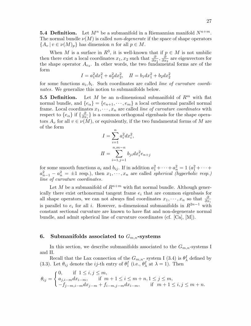
5.4 Definition. Let Mn be a submanifold in a Riemannian manifold Nn+m.The normal bundle ν(M) is called non-degenerate if the space of shape operatorsAv | v ∈ ν(M)p has dimension n for all p ∈ M .
When M is a surface in R3, it is well-known that if p ∈ M is not umbilicthen there exist a local coordinates x1, x2 such that ∂
∂x1, ∂
∂x2are eigenvectors for
the shape operator Ae3 . In other words, the two fundamental forms are of theform
I = a21dx2
1 + a22dx2
2, II = b1dx21 + b2dx2
2
for some functions ai, bi. Such coordinates are called line of curvature coordi-nates. We generalize this notion to submanifolds below.
5.5 Definition. Let M be an n-dimensional submanifold of Rm with flatnormal bundle, and eα = en+1, · · · , em a local orthonormal parallel normalframe. Local coordinates x1, · · · , xn are called line of curvature coordinates withrespect to eα if ∂
∂xi is a common orthogonal eigenbasis for the shape opera-
tors Av for all v ∈ ν(M), or equivalently, if the two fundamental forms of M areof the form
I =n∑
i=1
a2i dx2
i ,
II =n,m−n∑i=1,j=1
bjidx2i en+j
for some smooth functions ai and bij . If in addition a21 + · · ·+a2
n = 1 (a21 + · · ·+
a2n−1 − a2
n = ±1 resp.), then x1, · · · , xn are called spherical (hyperbolic resp.)line of curvature coordinates.
Let M be a submanifold of Rn+m with flat normal bundle. Although gener-ically there exist orthonormal tangent frame ei that are common eigenbasis forall shape operators, we can not always find coordinates x1, · · · , xn so that ∂
∂xi
is parallel to ei for all i. However, n-dimensional submanifolds in R2n−1 withconstant sectional curvature are known to have flat and non-degenerate normalbundle, and admit spherical line of curvature coordinates (cf. [Ca], [M]).
6. Submanifolds associated to Gm,n-systems
In this section, we describe submanifolds associated to the Gm,n-systems Iand II.
Recall that the Lax connection of the Gm,n- system I (3.4) is θIλ defined by
(3.3). Let θij denote the ij-th entry of θI1 (i.e., θI
λ at λ = 1). Then
θij =
0, if 1 ≤ i, j ≤ m,aj,i−mdxi−m, if m + 1 ≤ i ≤ m + n, 1 ≤ j ≤ m,−fj−m,i−mdxj−m + fi−m,j−mdxi−m, if m + 1 ≤ i, j ≤ m + n.

28
Set
ωi = θm+i,1 = a1idxi, ωij = θm+i,m+j = −fjidxj + fijdxi, if 1 ≤ i, j ≤ n,
ωn+i,n+j = θij = 0, if 1 ≤ i, j ≤ m,
ωi,n+j = θm+i,j = ajidxi, if 1 ≤ i ≤ n, 1 ≤ j ≤ m.
Since θI1 = (θij) is flat, we have
dωi = dθm+i,1
= −m∑
j=1
θm+i,j ∧ θj1 −n∑
j=1
θm+i,m+j ∧ θm+j,1
= −n∑
j=1
θm+i,m+j ∧ θm+j,1 = −n∑
j=1
ωij ∧ ωj .
If∑n
i=1 ω2i is non-degenerate, then (ωij) is the Levi-Civita connection 1-form
for the metric∑n
i=1 ω2i . Let E be a trivialization of θI
1 , i.e., E−1dE = θI1 .
Let en+i denote the i-th column of E for 1 ≤ i ≤ m, and let ei denote the(m + i)-th column of E, i.e., E = (en+1, · · · , en+m, e1, · · · , en). It follows fromdE = EθI
1 that en+1 is an n-dimensional submanifold in Sn+m−1 ⊂ Rn+m
such that en+1, en+2, · · · , en+m is a parallel normal frame and (x1, · · · , xn) is aspherical line of curvature coordinates such that the two fundamental forms are
I =n∑
i=1
a21idx2
i , II =n,m+n∑
i=1,α=n+1
a1iaα−n,idx2i eα.
We state this and the converse in the Theorem below.
6.1 Theorem. (Flat n-submanifolds in Sm+n−1). Let X be a local isometricimmersion of flat n-dimensional submanifold in Sn+m−1 with flat, non-degeneratenormal bundle, and m ≥ n. Let en+1 = X, and fix a local parallel normal frameen+2, · · · , en+m. Then:(i) There exist spherical line of curvature coordinates (x1, ..., xn) and a smooth
Mm×n-valued map A1 such that At1A1 = I and the first and second funda-
mental forms of X are given by
I =n∑
i=1
a21i dx2
i , II =n∑
i=1
m∑j=2
a1iajidx2i en+j . (6.1)
(ii) Let fij = (a1i)xj /a1j for i = j, fii = 0 for all 1 ≤ i, j ≤ n, and F = (fij) ∈gl∗(n). Then the Gauss, Codazzi and Ricci equations for the immersion X

29
is the Gm,n-system I (3.4) for (A1, F ). In other words, (A1, F ) is a solutionof (3.4).
(iii) Let ei = 1a1i
Xxi , g = (en+1, · · · , em+n, e1, · · · , en) ∈ O(m + n). Then
g−1dg =∑
i
(0 −A1Ci
CiAt1 −F tCi + CiF
)dxi, (6.2)
which is equal to the Lax connection (3.3) θIλ of equation (3.4) at λ = 1.
(iv) Conversely, if (A1, F ) is a solution of (3.4), then system (6.2) is solvable.Let g be a solution of (6.2), and X the first column g. If all entries of the firstrow of A1 are non-zero, then X is an isometric immersion of flat n-submanifoldsin Sn+m−1 with flat and non-degenerate normal bundle such that the two fun-damental forms are as in (i), where A1 = (aij).
PROOF.(i) can be proved the same way as for isometric immersions of n-submanifolds
in R2n−1 with constant sectional curvature −1 (cf. [Ca], [M]).From (i), we have
ωi = a1idxi, ωi,n+j = ajidxi, ωαβ = 0.
By Corollary 5.3, we get ωij = fijdxi −fjidxj . So g−1dg = (ωAB), and (ii), (iii)follow.
(iv) follows from the Fundamental Theorem of submanifolds in Euclideanspace.
When m = n, the above theorem was proved by Tenenblat in [Ten], whereequation (3.4) is called the generalized wave equation.
If we use a different parallel frame en+2, · · · , en+m for the immersion X inthe above Theorem, then there exists a constant matrix p = (pij) ∈ O(m − 1)such that en+i =
∑mj=2 pijen+j for 2 ≤ i ≤ m. The solution of (3.4) given by X
and parallel frame eα is (pA1, F ), where p =(
1 00 p
)and p = (pij).
Suppose (A, F ) is a solution of (3.4), and p ∈ O(m). By Corollary 3.5,(pA, F ) is also a solution of (3.4). As a consequence of Theorem 6.1 (iv), we get
6.2 Corollary. Let X, en+2, · · · , en+m, and (A1, F ) be as in Theorem 6.1, andc = (c1, · · · , cm) a unit vector. If all components of cA1 never vanish, thenY = c1X + c2en+2 + · · ·+ cmen+m is again an immersion of a flat n-submanifoldin Sn+m−1 with flat and non-degenerate normal bundle.
6.3 Theorem. (Flat n-submanifolds in Rn+m). Let n ≤ m, and X a localisometric immersion of flat n-dimensional submanifold in Rm+n with flat and

30
non-degenerate normal bundle. Fix a local parallel normal frame en+1, · · · , en+m.Then:(i) There exist a line of curvature coordinates (x1, ..., xn), a smooth Mm×n-
valued map A1 = (aij) and a smooth Mn×1-valued map b = (b1, ..., bn)such that At
1A1 = I and the first and second fundamental forms of X aregiven by
I =∑
i
b2i dx2
i , II =n∑
i=1
m∑j=1
biajidx2i en+j . (6.3)
(ii) Let fij = (bi)xj /bj for i = j, fii = 0, and F = (fij). Then (A1, F ) is asolution of the Gm,n-system I (3.4). Moreover, if
ei :=1bi
Xxi , g := (en+1, · · · , en+m, e1, · · · , en),
then
g−1dg =∑
i
(0 −A1Ci
CiAt1 −F tCi + CiF
)dxi,
which is the Lax connection θIλ defined by (3.3) for equation (3.4) at λ = 1.
(iii) Conversely, if (A1, F ) is a solution of (3.4) and b1, · · · , bn satisfy
(bi)xj = fijbj , 1 ≤ i = j ≤ n, (6.4)
then there exists a local isometric immersion of Rn in Rn+m such that thetwo fundamental forms are given by (6.3), where A1 = (aij) and F = (fij).
(iv) X lies in a hypersphere of radius 1 if and only if b = vA1 for some constantunit vector v ∈ M1×m.
PROOF. Statements (i), (ii) and (iii) follows from an argument similar tothose for Theorem 6.1. To prove (iv), we assume ‖X−X0‖ = 1 for some constantvector X0. Then X−X0 is a parallel normal field, which implies that there existsconstant unit vector v = (v1, · · · , vm) such that X − X0 =
∑i vien+i. Hence
d(X − X0) = dX =∑
i
viden+i =∑
i
viωj,n+iej =∑
i
viaijdxjej .
But dX =∑
j bjdxjej . So b = vA1. The converse can be proved by reversingthe argument.
6.4 Remark. System (6.4) was studied by Darboux [Da]. It can be solved ifand only if
(fij)xk= fikfkj , i, j, k distinct. (6.5)

31
This condition is obtained by equating (bi)xjxk= (bi)xkxj :
(bi)xjxk= (fijbj)xk
= (fij)xkbj + fijfjkbk
= (fikbk)xj= (fik)xj
bk + fikfkjbj .
Moreover, the space of solutions of (6.4) depends on n arbitrary smooth functionsof one variable. In fact, if ξ(t) = (ξ1(t), · · · , ξn(t)) is a curve from (−ε, ε) to Rn
such that ξ′i(t) never vanishes for all 1 ≤ i ≤ n, then given any smooth mapsb01, · · · , b0
n : (−ε, ε) → R there exists a unique solution (b1, · · · , bn) of (6.4) suchthat bi(ξ(t)) = b0
i (t). The compatibility condition (6.5) is the third equation of(3.4). So (b1, · · · , bn) in Theorem 6.3 (iii) always exists.
We can use a proof similar to that of the previous theorem to deduce:
6.5 Theorem. (Local isometric immersion of Sn in Sn+m). Suppose X is alocal isometric immersion of Sn in Sn+m with flat and non-degenerate normalbundle, and eα is a parallel normal frame. Then:
(i) There exist a local coordinate system (x1, . . . , xn), a smooth M0m×n-valued
map A1 = (aij) and a smooth Mn×1-valued map b = (b1, · · · , bn)t suchthat the two fundamental forms of X are given by
I =∑
i
b2i dx2
i , II =n,m∑
i=1,j=1
ajibidx2i en+j . (6.6)
(ii) Let fij = (bi)xj/bj if i = j, fii = 0 for all 1 ≤ i ≤ n, and F = (fij). Then
(A1, F, b) is a solution of the partial Gm,n+1-system I (3.14).
(iii) Let ei = 1bi
Xxi, and g = (en+1, · · · , en+m, e1, · · · , en, X). Then
g−1dg =∑
i
( 0 −A1Ci 0CiA
t1 −F tCi + CiF Cib
0 −btCi 0
)dxi, (6.7)
which is the Lax connection Θλ defined in (3.13) for system (3.14) at λ = 1.
(iv) If (A1, F, b) is a solution of (3.14), then system (6.7) is solvable. Let g bea solution of (6.7), and let X denote the last column of g. Then X is a localisometric immersion of Sn in Sn+m.
Next we study submanifolds associated to the Gm,n- system II (3.10). Wewill show that each solution of (3.10) gives rise to an O(n)-family of submanifoldswith common line of curvature coordinates. In order to simplify the notation, wemake the following definition:

32
6.6 Definition. Let m > n, O a domain in Rn, and Xi : O → Rm an immer-sion with flat and non-degenerate normal bundle for 1 ≤ i ≤ n. (X1, · · · , Xn) iscalled a n-tuple in Rm of type O(n) (O(n − 1, 1) resp.) if
(i) the normal plane of Xi(x) is parallel to the normal plane of Xj(x) for all1 ≤ i, j ≤ n and x ∈ O,
(ii) there exists a common parallel normal frame eαmα=n+1,
(iii) x ∈ O is a spherical (hyperbolic resp.) line of curvature coordinate system(cf. Definition 5.5) with respect to eα for each Xi such that the fundamentalforms for Xj are
Ij =n∑
i=1
b2jidx2
i ,
IIj =n,m−n∑i=1,k=1
bjigkidx2i en+k
(6.8)
for some O(n)-valued ((O(n − 1, 1)- resp.) map B = (bij) and a M(m−n)×n-valued map G = (gij).
We note that an n-tuple in Rm of type O(n) or O(n − 1, 1) is an n-tupleof parametrized n-dimensional submanifolds in Rm and the parametrization is aspherical or hyperbolic line of curvature coordinates.
6.7 Theorem. Let (X1, · · · , Xn) be an n-tuple in Rm of type O(n), en+1, · · ·,em common parallel normal frame, and (x1, · · · , xn) a common spherical line ofcurvature coordinates for all Xj ’s such that the two fundamental forms Ij , IIj forXj are given by (6.8). Set fij = (b1j)xi/b1i if i = j, fii = 0, and F = (fij). If allentries of G are nonzero, then (F, G, B) is a solution of (3.10), the Gm,n-systemII.
PROOF. It follows from the definition of n-tuples that
ω(j)1 = bj1dx1, ω
(j)2 = bj2dx2, · · · , ω(j)
n = bjndxn
is a dual 1-frame for Xj , and ω(j)i,n+k = gkidxi for each Xj . Note that ω
(j)i,n+k is
independent of j. By Corollary 5.3, the Levi-Civita connection 1-form for themetric Ij is
ω(j)ik = −f
(j)ik dxk + f
(j)ki dxi, where f
(j)ik =
(bjk)xi
bji.
Since
dω(j)i,n+k = −
n∑r=1
ω(j)ir ∧ ω
(j)r,n+k
for 1 ≤ k ≤ m−n and gk1, · · · , gkn are non-zero, Cartan’s Lemma and Corollary5.3 imply that
f(j)ir =
(gkr)xi
gki,

33
which is independent of j. Hence
ω(j)ij = ω
(1)ij = −fijdxj + fjidxi.
The structure equation, Gauss-Codazzi-Ricci equations for X1, · · · , Xn implythat (F, G, B) is a solution of (3.10).
The converse is also true:
6.8 Theorem. (n-tuples in Rm of type O(n)). Suppose (F, G, B) : Rn →gl∗(n) ×M(m−n)×n × O(n) is a solution of the Gm,n-system II (3.10). Let
F = (fij), G = (gij), B = (bij).
Then:(i)
τ =n∑
i=1
(−FCi + CiF
t CiGt
−GCi 0
)dxi
is a flat o(m)-valued connection 1-form. Hence there exists A : Rn → O(m)such that
A−1dA = τ =n∑
i=1
(−FCi + CiF
t CiGt
−GCi 0
)dxi. (6.9)
(ii) Write A = (A1, A2) with A1 ∈ Mm×n and A2 ∈ Mm×(m−n). Then
n∑i=1
A1CiBtdxi
is exact. So there exists a map X : Rn → Mm×n such that
dX = −n∑
i=1
A1CiBtdxi. (6.10)
(iii) Suppose all the entries of B are non-zero. Let Xj : Rn → Rm denote thej-th column of X (solution of (6.10)), and ei denote the i-th column of A.Then (X1, · · · , Xn) is an n-tuple in Rm of type O(n). In fact,(1) e1, · · · , en are tangent to Xj for all 1 ≤ j ≤ n; so the tangent planes of
X1, · · · , Xn are parallel,(2) en+1, · · · , em is a parallel normal frame for each Xj ,(3) the two fundamental forms for the immersion Xj are
Ij =n∑
i=1
b2jidx2
i ,
IIj = −n,m−n∑i=1,k=1
gkibjidx2i en+k.
(6.11)

34
PROOF. By Proposition 3.7, θIIλ defined by (3.9) is flat for all λ ∈ C. In
particular,
θII0 =
(τ 00 0
)is flat.
The gauge transformation of θIIλ by
(A 00 I
)is
(A 00 I
)∗ θII
λ =n∑
i=1
(0 −λA1CiB
t
λBCiAt1 0
), (6.12)
which is flat for all λ ∈ C. It follows from Proposition 2.6 that∑n
i=1 A1CiBtdxi
is exact. This proves (ii).Equate the j-th column of equation (6.10) to get
dXj = −n∑
k=1
bjkekdxk.
So Ij =∑
k b2jkdx2
k. The rest of (iii) follows from the fact that A−1dA = τ .
6.9 Corollary. Let (X1, · · · , Xn) be an n-tuple in Rm of type O(n), and p ∈O(m) and q ∈ O(n) constant matrices. Then p(X1, · · · , Xn)q is also an n-tuplein Rm of type O(n).
PROOF. We call a local orthonormal frame A = (e1, · · · , em) an adaptedframe for the n-tuple (X1, · · · , Xn) of type O(n) if e1, · · · , en are common prin-cipal curvature directions and en+1, · · · , em are a common parallel normal framefor each Xj . By Theorem 6.7, there exist G and B such that (F, G, B) is a so-lution of system (3.10). A direct computation shows that Xq is an n-tuple withAq as an adapted frame and the corresponding solution of (3.10) is the same(F, G, B).
Note that if A is a solution of (6.9), then so is pA. By Theorem 6.8 (ii), pXis an n-tuple of type O(n) in Rm.
The immersion Xj in Theorem 6.8 can be obtained either by solving thesystem (6.10) using integration or by an analogue of Sym’s formula (cf. [Sy])below.
6.10 Proposition. Suppose θ(x, λ) = α1(x)λ + α0(x) is a flat G-valued con-nection 1-form on x ∈ Rn, and E(x, λ) is a trivialization of θ(x, λ), i.e., E−1dE =θ. Set
Y (x) =∂E
∂λ(x, 0)E−1(x, 0).
Then dY = E(x, 0)α1(x)E(x, 0)−1.

35
PROOF. A direct computation gives
dY =(
∂
∂λ(dE)
)E−1 − ∂E
∂λE−1dEE−1
∣∣∣∣λ=0
=(
∂
∂λ(Eθ)
)E−1
∣∣∣∣λ=0
− ∂E
∂λ(x, 0)θ(x, 0)E(x, 0)−1
= E(x, 0)α1(x)E(x, 0)−1.
6.11 Corollary. Let E(x, λ) be a frame for a solution ξ of the Gm,n-system(3.1), and
Y (x) =∂E
∂λ(x, 0)E−1(x, 0).
Then:
(i) Y =(
0 X−Xt 0
)for some X ∈ Mm×n.
(ii) X = (X1, · · · , Xn) is an n-tuple in Rm of type O(n).(iii) dX = −A1δB
t, where δ = diag(dx1, · · · , dxn). In other words, X satisfies(6.10)
PROOF. Since E satisfies the reality condition, E(x, 0) ∈ O(m) × O(n).
Write E(x, 0) =(
A(x) 00 B(x)
)and set
δ = diag(dx1, · · · , dxn), β =(
δ0
).
It follows from Proposition 6.10 and the fact that the Lax connection of (3.1) isθ(x, λ) = α0λ + α1 with
α1 =(
0 −A1δBt
BδAt1 0
),
that
dY = E(x, 0)(
0 −ββ 0
)E(x, 0)−1 =
(0 −A1δB
t
BδAt1 0
).
So dX = −A1δBt, i.e., X solves (6.10).
We end this section by studying the Gm,2-system II (3.10).
6.12 Proposition. The Gm,2-system II (3.10) is the Gauss-Codazzi equationsfor a surface in Rm that admits spherical line of curvature coordinates.

36
PROOF. Suppose M is a surface in Rm, which admits a spherical lineof curvature coordinate system (x1, x2) with respect to a parallel normal framee3, · · · , em. Then there exist a function u and a M(m−2)×2 -valued map G = (gij)such that
I = cos2 u dx21 + sin2 u dx2
2,
II =m−2∑j=1
(gj1 cos u dx21 + gj2 sinu dx2
2)e2+j .
The Gauss-Codazzi-Ricci equations are the following system for u, gj1, gj2:
ux1x1 − ux2x2 +∑m−2
i=1 gi1gi2 = 0,(gi2)x1 = gi1ux1 ,(gi1)x2 = −gi2ux2 .
(6.13)
Let
B =(
cos u sinu− sinu cos u
), F =
(0 ux1
−ux2 0
), G = (gij). (6.14)
Then (F, G, B) is a solution of the Gm,2 system II (3.10).Conversely, if (F, G, B) is a solution of the Gm,2-system II (3.10), then
we may assume B =(
cos u sinu− sinu cos u
). If sinu cos u = 0, then by the third
equation of (3.10), we have f12 = ux1 and f21 = −ux2 , i.e., F =(
0 ux1
−ux2 0
).
Let gij denote the ij-th entry of G. Then system (3.10) is system (6.13).
6.13 Corollary. Let X1 : O → Rm be an immersion and (x, y) ∈ O thespherical line of curvature coordinates with respect to a parallel normal framee3, · · · , em. Then there exists an immersion surface X2 unique up to translationsuch that (X1, X2) is a 2-tuple in Rm of type O(2). Moreover, the fundamentalforms of X1, X2 are respectively given by
I1 = cos2 u dx21 + sin2 u dx2
2, II1 =m∑
j=1
(gj1 cos u dx21 + gj2 sinu dx2
2)e2+j ,
I2 = sin2 u dx21 + cos2 u dx2
2, II2 =m−2∑j=1
(−gj1 sinu dx21 + gj2 cos u dx2
2)e2+j .
(6.15)
It follows from the Gauss equation (5.3) that
K1 = −K2 =
∑m−2j=1 gj1gj2
sinu cos u.
So we have

37
6.14 Corollary. Let O be an open subset of R2, (X1, X2) : O → Rm × Rm
a 2-tuple in Rm of type O(2), and (x1, x2) ∈ O spherical line of curvaturecoordinates. Then
K2(x) = −K1(x),
where K1, K2 are respectively the Gaussian curvature of X1, X2.
6.15 Definition. If (M1, M2) is a 2-tuple in Rm of type O(2) (O(1, 1) resp.)with a parallel normal frame e3, · · · , em and spherical line of curvature coordi-nates, then we call M2 a C-dual of M1. Note that any two C-duals of M1 arediffered by a translation.
6.16 Example. Recall that given a surface M in R3 with curvature −1, thereexist spherical line of curvature coordinates x1, x2 such that the two fundamentalforms are
I = cos2 u dx21 + sin2 u dx2
2,
II = sinu cos u (dx21 − dx2
2),
and u satisfiesux1x1 − ux2x2 = sinu cos u. (SGE)
This implies that (u, sinu,− cos u) is a solution of (6.13). Let X(x1, x2) denotethe immersion of M . Then (X, e3) is a 2-tuple in R3 of type O(2), where e3 isthe unit normal of M , which is an open subset of S2.
7. Submanifolds associated to G1m,n- systems
In this section, we describe submanifolds whose fundamental equations aregiven by G1
m,n-systems.Let Rk,1 denote the Lorentz space equipped with the non-degenerate bilinear
form of index one:
〈x, y〉1 = x1y1 + . . . + xkyk − xk+1yk+1.
The moving frame computation for submanifolds in Rk,1 can be carried out in asimilar way as for submanifolds in Rk+1 except that the Levi-Civita connection1-form (ωij) of the flat Lorentzian metric 〈, 〉1 is o(k, 1)-valued.
Let Hk denote the k-dimensional simply connected space form of sectionalcurvature -1 (i.e., a hyperbolic k-space). It is well-known that
x ∈ Rk,1 | 〈x, x〉1 = −1, xk+1 > 0
with the induced metric is isometric to Hk. We need the following Propositionlater, which can be proved using a direct computation (cf. Chap. 2 of [PT]).

38
7.1 Proposition. Let v0 ∈ Rk,1 be a constant non-zero vector, c ∈ R a con-stant, and Nv,c the hypersurface defined by
Nv0,c = x ∈ Hk | 〈x, v0〉1 = c.
Then Nv,c is a totally umbilic hypersurface of Hk with constant sectional curva-ture
−〈v0, v0〉1c2 + 〈v0, v0〉1
.
We use methods similar to those in section 6 to find submanifolds whosefundamental equations are the various G1
m,n-systems. For the G1m,n-system I, let
(θij) denote the connection 1-form θIλ defined by (4.3) at λ = 1. Then (θij) is a
o(m + n, 1)-valued 1-form and θm+i,m+j = −εiεjfjidxj + fijdxi, 1 ≤ i, j ≤ n + 1,θm+i,α = aαidxi, 1 ≤ i ≤ n + 1, 1 ≤ α ≤ m,θαβ = 0, 1 ≤ α, β ≤ m,
where ε1 = · · · = εn = −εn+1 = 1. Letωij = θm+i,m+j , 1 ≤ i, j ≤ n + 1,ωiα = θm+i,α, 1 ≤ i ≤ n + 1, 1 ≤ α ≤ m,ωαβ = θαβ , 1 ≤ α, β ≤ m.
Then the flatness of (θij) is exactly the Gauss-Codazzi-Ricci equations for (n+1)-dimensional flat, Lorentzian submanifolds in Rn+m,1. So we get
7.2 Theorem. (Local isometric immersions of Rn,1 in Rm+n,1). Let X be alocal isometric immersion of Rn,1 in Rn+m,1 with flat and non-degenerate normalbundle. Fix a local parallel normal frame en+2, · · · , en+m+1. Then:(i) There exist a line of curvature coordinates (x1, ..., xn+1) and a Mm×(n+1)-
valued map A1 = (aij) and a map b = (b1, ..., bn+1) such that At1A1 = I
and the first and second fundamental forms of X are given by
I =n+1∑i=1
εib2i dx2
i , II =n+1∑i=1
m−n∑j=2
biajidx2i en+j , (7.1)
where ε1 = · · · = εn = −εn+1 = 1.(ii) Let fij = (bi)xj /bj for i = j, fii = 0, and F = (fij). Then (A1, F ) is a
solution of the G1m,n-system I (4.4).
(iii) Conversely, if (A1, F ) is a solution of (4.4) and b1, · · · , bn+1 satisfies (bi)xj =fijbj for all i = j, then there exists a local isometric immersion of Rn,1 in Rm+n,1
such that the two fundamental forms are given by (7.1), where A1 = (aij) andF = (fij).

39
Next we consider the partial G1m,n-system I of n variables, system (4.10).
Let θij denote the ij-th entry of τ Iλ , defined by (4.9), at λ = 1. So we have
θαβ = 0, 1 ≤ α, β ≤ m,θm+i,m+j = −fjidxj + fijdxi, 1 ≤ i, j ≤ n,θm+i,α = aαidxi, 1 ≤ i ≤ n, 1 ≤ α ≤ m,θm+i,m+n+1 = bidxi, 1 ≤ i ≤ n.
Let
ωi = θm+i,m+n+1, 1 ≤ i ≤ n,ωij = θm+i,m+j , if 1 ≤ i, j ≤ n,ωi,n+j = θm+i,j , if 1 ≤ i ≤ n, 1 ≤ j ≤ m,ωn+i,n+j = θij , if 1 ≤ i, j ≤ m.
Then system (4.10) (given by the flatness of τ I1 ) is exactly the Gauss-Codazzi-
Ricci equations for local isometric immersions of Hn in Hn+m ⊂ Rn+m,1 withflat and non-degenerate normal bundle. We summarize this below.
7.3 Theorem. (Local isometric immersion of Hn in Hn+m). Let X be a localisometric immersion of Hn in Hn+m with flat and non-degenerate normal bundle,and eα a parallel normal frame. Then:(i) There exist a line of curvature coordinate system (x1, . . . , xn), a Mm×n-
valued map A1 = (aij) satisfying At1A1 = I, and a Mn×1-valued map
b = (b1, · · · , bn)t such that the two fundamental forms of X are given by
I =∑
i
b2i dx2
i , II =n,m−n∑i=1,j=1
ajibidx2i en+j . (7.2)
(ii) Let fij = (bi)xj /bj if i = j, fii = 0 for all 1 ≤ i ≤ n, and F = (fij). Then
(A1, F, b) is a solution of the partial G1m,n-system (4.10).
(iii) Let ei = 1bi
Xxi, and g = (en+1, · · · , en+m, e1, · · · , en, X). Then
g−1dg =∑
i
( 0 −A1Ci 0CiA
t1 −F tCi + CiF Cib
0 btCi 0
)dxi, (7.3)
which is equal to the Lax connection τ Iλ defined in (4.9) for system (4.10) at
λ = 1.(iv) If (A1, F, b) is a solution of (4.10), then system (7.3) is solvable.(v) Let g be a solution of (7.3). Then the last column of g is an isometric
immersion of a constant sectional curvature −1 submanifold of Hn+m.(vi) Mn lies in a totally umbilic hypersurface of Hn+m if and only if there isa constant vector w ∈ Mm×1 such that b = At
1w. Moreover, Mn lies in a flattotally umbilic hypersurface if and only if ‖w‖ = 1.

40
PROOF. Statements (i)-(v) follows from standard submanifold theory. Toprove (vi), note that every umbilic hypersurface of Hn+m is the intersection ofHn+m with a hyperplane (cf. [PT]), i.e., it is of the form
Nv,c = x ∈ Hn+m | 〈x, v〉1 = c
for some constant v ∈ Rn+m,1 and c ∈ R. By Proposition 7.1, Nv,c has constantsectional curvature
− 〈v, v〉1c2 + 〈v, v〉1
.
Suppose the image of X lies in Nv,c. Then < dX, v >1= 0, which implies that vis normal to X. But v is constant, so v is a parallel normal vector field of M asa submanifold of Rn+m,1. Hence
v =m∑
k=1
vken+k + vm+1X (7.4)
for some constants v1, · · · , vm+1. It follows from 〈X, v〉1 = c and 〈X, X〉1 = −1that vm+1 = −c. Differentiate (7.4) to get
cωi = cbidxi =m∑
k=1
vkωi,n+k =m∑
k=1
vkakidxi,
socbi =
∑vkaki. (7.5)
Let v = (v1, · · · , vm)t, and w = v/c. Then (7.5) implies that b = At1w. Since
〈v, v〉1 = ‖ v ‖ 2 − c2, it follows from the formula for the sectional curvature thatNv,c is flat if and only if 〈v, v〉1 = 0, i.e., ‖ v ‖ 2 = c2, or equivalently, ‖w ‖ = 1.
For m = n, the above theorem was proved by Terng in [Te2].
7.4 Theorem. ((n + 1)-tuples in Rm of type O(n, 1)). Suppose m > n + 1,and
(F, G, B) : Rn+1 → gl∗(n + 1) ×M(m−n−1)×(n+1) × O(n, 1)
is a solution of the G1m,n-system II (4.6). Let F = (fij), G = (gij), and B = (bij).
Then:(i)
ω =n+1∑i=1
(−FCi + CiF
t CiGt
−GCi 0
)dxi (7.6)
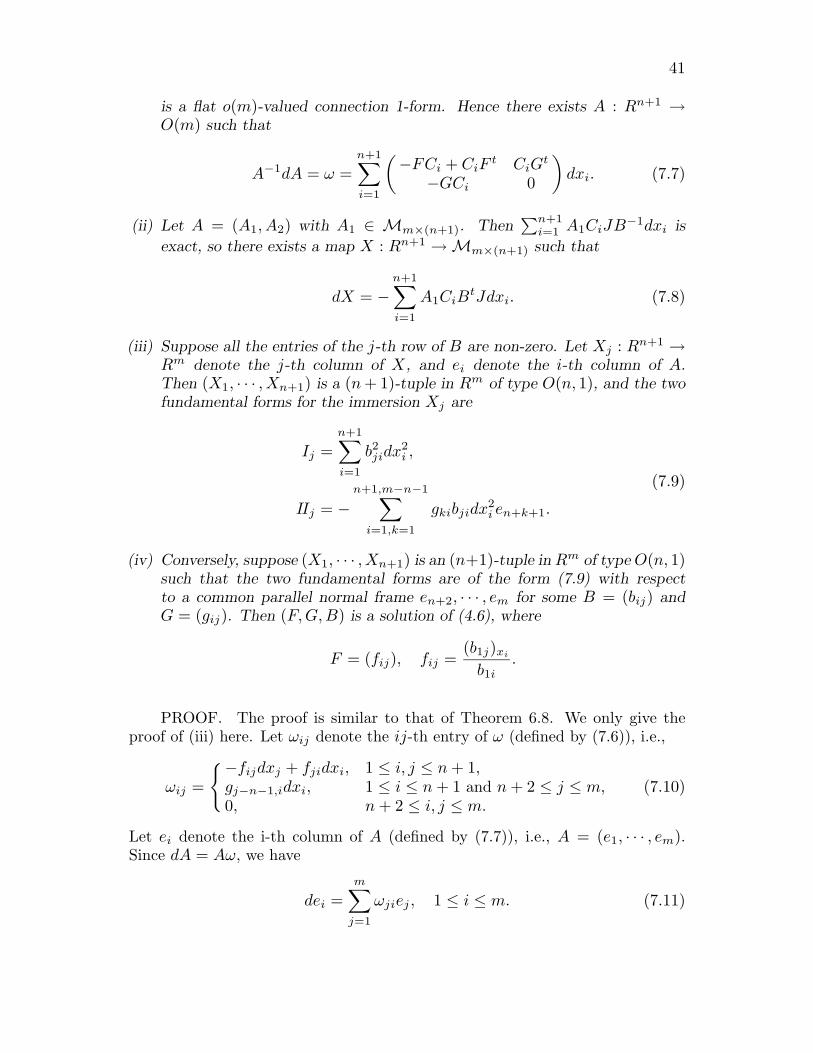
41
is a flat o(m)-valued connection 1-form. Hence there exists A : Rn+1 →O(m) such that
A−1dA = ω =n+1∑i=1
(−FCi + CiF
t CiGt
−GCi 0
)dxi. (7.7)
(ii) Let A = (A1, A2) with A1 ∈ Mm×(n+1). Then∑n+1
i=1 A1CiJB−1dxi is
exact, so there exists a map X : Rn+1 → Mm×(n+1) such that
dX = −n+1∑i=1
A1CiBtJdxi. (7.8)
(iii) Suppose all the entries of the j-th row of B are non-zero. Let Xj : Rn+1 →Rm denote the j-th column of X, and ei denote the i-th column of A.Then (X1, · · · , Xn+1) is a (n + 1)-tuple in Rm of type O(n, 1), and the twofundamental forms for the immersion Xj are
Ij =n+1∑i=1
b2jidx2
i ,
IIj = −n+1,m−n−1∑
i=1,k=1
gkibjidx2i en+k+1.
(7.9)
(iv) Conversely, suppose (X1, · · · , Xn+1) is an (n+1)-tuple in Rm of type O(n, 1)such that the two fundamental forms are of the form (7.9) with respectto a common parallel normal frame en+2, · · · , em for some B = (bij) andG = (gij). Then (F, G, B) is a solution of (4.6), where
F = (fij), fij =(b1j)xi
b1i.
PROOF. The proof is similar to that of Theorem 6.8. We only give theproof of (iii) here. Let ωij denote the ij-th entry of ω (defined by (7.6)), i.e.,
ωij =
−fijdxj + fjidxi, 1 ≤ i, j ≤ n + 1,gj−n−1,idxi, 1 ≤ i ≤ n + 1 and n + 2 ≤ j ≤ m,0, n + 2 ≤ i, j ≤ m.
(7.10)
Let ei denote the i-th column of A (defined by (7.7)), i.e., A = (e1, · · · , em).Since dA = Aω, we have
dei =m∑
j=1
ωjiej , 1 ≤ i ≤ m. (7.11)

42
By Theorem 7.4 (ii),
dXr = −n+1∑i=1
briεreidxi, (7.12)
where Xr is the r-th column of X. So e1, · · · , en+1 is a common orthonormaltangent frame, and
ω(r)1 = −εrbr1dx1, · · · , ω(r)
n+1 = −εrbr,n+1dxn+1
is the dual coframe for Xr. Since
ω(r)i,n+1+j = 〈den+1+j , ei〉1 = ωi,n+j+1 = gjidxi,
en+2, · · · , em is a common parallel normal frame and (x1, · · · , xn+1) is a hy-perbolic line of curvature coordinate system for each Xr.
7.5 Corollary. Let (X1, · · · , Xn+1) be a (n + 1)-tuple in Rm of type O(n, 1),and p ∈ O(m), q ∈ O(n, 1) constant matrices. Then p(X1, · · · , Xn+1)q is also a(n + 1)-tuple in Rm of type O(n, 1).
7.6 Corollary. Let v be a solution of the G1m,n-system (4.2), E a frame for v,
and Y = (∂E∂λ E−1)(x, 0). Then:
(i) Y =(
0 X−JXt 0
)for some Mm×(n+1)-valued map X and J = In,1 =
diag(1, · · · , 1,−1).(ii) X = (X1, · · · , Xn) is an (n+1)-tuple in Rm of type O(n, 1).
8. G1m,1-systems and isothermic surfaces
We study the relation between the G1m,1-system and isothermic surfaces in
Rm.
8.1 Proposition. The G1m,1-system II (4.6) is the Gauss-Codazzi-Ricci equa-
tions for surfaces in Rm admitting hyperbolic line of curvature coordinates.
PROOF. Let O be a domain in R2, X : O → Rm an immersion with flatand non-degenerate normal bundle, and (x1, x2) ∈ O a hyperbolic line of curva-ture coordinate system with respect to the parallel normal frame e3, · · · , em.Then there exist u and gki for 1 ≤ k ≤ m − 2 and i = 1, 2 such that the twofundamental forms are
I = cosh2 u dx21 + sinh2 u dx2
2,
II =m−2∑k=1
(gk1 cosh u dx21 + gk2 sinhu dx2
2)ek+2.(8.1)

43
The Gauss-Codazzi-Ricci equations for X are
ux1x1 + ux2x2 +∑m−2
k=1 gk1gk2 = 0,(gk1)x2 = ux2gk2,(gk2)x1 = ux1gk1.
(8.2)
This is exactly the G1m,1-system (4.6) for (F, G, B), where
F =(
0 ux1
ux2 0
), G = (gki), B =
(cosh u sinhusinhu cosh u
)∈ O(1, 1). (8.3)
Conversely, if (F, G, B) is a solution of the G1m,1-system (4.6), then since
B ∈ O(1, 1) we may assume
B =(
cosh u sinhusinhu cosh u
).
The third equation of (4.6) implies that f12 = ux1 and f21 = ux2 , i.e., (F, G, B)is of the form (8.3). Write equation (4.6) for (F, G, B) in terms of u and gki toget equation (8.2). This completes the proof.
8.2 Corollary. Let O be a domain of R2, and X1 : O → Rm an immersionwith flat normal bundle and (x, y) ∈ O a hyperbolic line of curvature coordinatesystem with respect to a parallel normal frame e3, · · · , em. Then there exists animmersion X2 unique up to translation such that (X1, X2) is a 2-tuple in Rm oftype O(1, 1). Moreover, the fundamental forms of X1, X2 are given respectivelyby
I1 = cosh2 u dx21 + sinh2 u dx2
2,
II1 =∑m−2
j=1 (gj1 cosh u dx21 + gj2 sinhu dx2
2)e2+j ,I2 = sinh2 u dx2
1 + cosh2 u dx22,
II2 =∑m−2
j=1 (−gj1 sinhu dx21 − gj2 cosh u dx2
2)e2+j .
(8.4)
Let K1, K2 denote the Gaussian curvature of X1 and X2 respectively. TheGauss equation implies that
K1 = K2 =∑m−2
k=1 gk1gk2
sinhu cosh u.
Hence we get
8.3 Corollary. Let (X1, X2) : O → Rm be a 2-tuple in Rm of type O(1, 1)such that (x1, x2) ∈ O is a hyperbolic line of curvature coordinate system. Then
K2(x) = K1(x)
where K1, K2 are respectively the Gaussian curvature of X1, X2.

44
Next we describe the relation between 2-tuple in Rm of type O(1, 1) andisothermic surfaces in Rm. The following definition, given by Burstall in [Bu],generalizes the classical notion of isothermic surfaces in R3 ([Da]).
8.4 Definition. Let O be a domain in R2. An immersion X : O → Rm iscalled isothermic if it has flat normal bundle and the two fundamental forms areof the form
I = e2u(dx21 + dx2
2), II =m−2∑k=1
eu(gk1dx21 + gk2dx2
2)e2+k
with respect to some parallel normal frame e3, · · · , em, or equivalent (x1, x2) ∈ Ois conformal and line of curvature coordinate system for X.
A direct computation gives
8.5 Proposition. The Gauss-Codazzi-Ricci equation for isothermic surfaces inRm is (8.2).
It was first noted by Cieslinski, Goldstein and Sym in [CGS] that equationfor isothermic surfaces in R3 has a Lax pair. There have been many papers([Ci], [BHPP], [Bu], [HP], [HMN]) using techniques from solition theory to studyisothermic surfaces in 3-space.
Next we give a simple relation between isothermic surfaces in Rm and 2-tuples in Rm of type O(1, 1).
8.6 Proposition. Suppose (X1, X2) is a 2-tuple in Rm of type O(1, 1). LetY1 = X1 − X2 and Y2 = X1 + X2. Then both Y1 and Y2 are isothermic.
PROOF. Let (u, (gij)) be the solution of (8.2) associated to (X1, X2). Weuse the same notations as in Theorem 7.4. Write X = (X1, X2). By (7.12), weget
dX1 = − cosh u dx1e1 − sinhu dx2e2,dX2 = sinhu dx1e1 + cosh u dx2e2.
Note that
F =(
0 ux1
ux2 0
), ω12 = ux2dx1 − ux1dx2, ωi,2+j = gjidxi.
Use (7.11) to get
∇e1 = ω21e2 = (ux2dx1 − ux1dx2)e2,∇e2 = ω12e1 = −(ux2dx1 − ux1dx2)e1,dek+2 = ω1,k+2e1 + ω2,k+2e2 = gk1dx1e1 + gk2dx2e2.
Compute directly to get
dY1 = dX1 − dX2 = −(cosh u + sinhu)(dx1e1 + dx2e2).

45
So the induced metric for Y1 is e2u(dx21 + dx2
2). Similarly, we can get explicitformula for dY2 and dek for 3 ≤ k ≤ m. This computation implies that the twofundamental forms for Y1 and Y2 are
I1 = e2u(dx2
1 + dx22),
II1 = −eu∑m−2
k=1 (gk1dx21 + gk2dx2
2)e2+k,(8.5)
I2 = e−2u(dx2
1 + dx22),
II2 = e−u∑m−2
k=1 (−gk1dx21 + gk2dx2
2)e2+k.(8.6)
Hence Y1 and Y2 are isothermic surfaces.
We call (Y1, Y2) an isothermic pair . If (u, gk1, gk2) is the solution of (8.2)corresponding to Y1, then (−u, gk1,−gk2) is the solution of (8.2) correspondingto Y2. For m = 3, the transformation from Y1 to Y2 is the classical Christoffeltransformation. Burstall generalizes this result to arbitrary m in [Bu]. In fact, hedeveloped in [Bu] a beautiful theory of isothermic surfaces in Rm and explainedits relation to conformal geometry, Clifford algebra and the curved flat systemassociated to G1
m,1. His result motivated us to study the Gm,n-system II andG1
m,n-system II for general m, n.Next we describe the o(m + 1, 1) model used by Burstall, Jeromin, Pedit
and Pinkall [BHPP] for m = 3 and by Burstall [Bu] for general m ≥ 3. Let
σk,1 =(
Ik−1 00 σ1,1
), rk,1 =
(Ik−1 0
0 r1,1
),
where σ1,1 =(
0 11 0
), r1,1 =
1√2
(1 1−1 1
).
Note that the bilinear form defined by σk,1 and Ik,1 are isometric, and
rtk,1σk,1rk,1 = Ik,1.
LetOσ(k, 1) = ξ ∈ GL(k + 1) | ξtσξ = σ.
Then φk,1(g) = rtk,1grk,1 is a group isomorphism from O(k, 1) to Oσ(k, 1). If
we replace θIIλ by ΩII
λ = (φm+1,1)∗(θIIλ ) in Theorem 7.4, then the integration in
Theorem 7.4 (ii) gives an isothermic pair Y = (Y1, Y2).
The following proposition, which states that a CMC surface in R3 withoutumbilic points admits isothermic coordinates, is well-known (for a proof see [PT]).
8.7 Proposition. Let M be an immersed surface without umbilic points inspace form N3(c), and k1, k2 the principal curvature functions. If M has constant
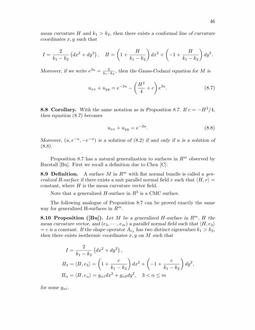
46
mean curvature H and k1 > k2, then there exists a conformal line of curvaturecoordinates x, y such that
I =2
k1 − k2
(dx2 + dy2
), II =
(1 +
H
k1 − k2
)dx2 +
(−1 +
H
k1 − k2
)dy2.
Moreover, if we write e2u = 2k1−k2
, then the Gauss-Codazzi equation for M is
uxx + uyy = e−2u −(
H2
4+ c
)e2u. (8.7)
8.8 Corollary. With the same notation as in Proposition 8.7. If c = −H2/4,then equation (8.7) becomes
uxx + uyy = e−2u. (8.8)
Moreover, (u, e−u,−e−u) is a solution of (8.2) if and only if u is a solution of(8.8).
Proposition 8.7 has a natural generalization to surfaces in Rm observed byBurstall [Bu]. First we recall a definition due to Chen [C]:
8.9 Definition. A surface M in Rm with flat normal bundle is called a gen-eralized H-surface if there exists a unit parallel normal field v such that 〈H, v〉 =constant, where H is the mean curvature vector field.
Note that a generalized H-surface in R3 is a CMC surface.
The following analogue of Proposition 8.7 can be proved exactly the sameway for generalized H-surfaces in Rm.
8.10 Proposition ([Bu]). Let M be a generalized H-surface in Rm, H themean curvature vector, and (e3, · · · , em) a parallel normal field such that 〈H, e3〉= c is a constant. If the shape operator Ae3 has two distinct eigenvalues k1 > k2,then there exists isothermic coordinates x, y on M such that
I =2
k1 − k2
(dx2 + dy2
),
II3 = 〈II, e3〉 =(
1 +c
k1 − k2
)dx2 +
(−1 +
c
k1 − k2
)dy2,
IIα = 〈II, eα〉 = gα1dx2 + gα2dy2, 3 < α ≤ m
for some gαi.

47
We call the isothermic coordinates x, y in the above Proposition the canonicalisothermic coordinates for the generalized H-surface M .
The following Proposition generalizes the classical Bonnet transformationfor CMC surfaces in R3. The proof follows from a direct computation as in theclassical case.
8.11 Proposition ([Bu]). Let O be a domain in R2, Y : O → Rm an isother-mic immersion of a generalized H-surface in Rm, (x1, x2) ∈ O the canonicalisothermic coordinates, and e3 the parallel unit normal field such that 〈H, e3〉 =2c is a constant. Then:
(i) If c = 0, then (Y, Y − 1ce3) is an isothermic pair.
(ii) If c = 0, then (Y, e3) is an isothermic pair.
Next we study the class of solutions of the G13,1-system II corresponding to
isothermic immersions of minimal surface in R3. If Y is an isothermic immersionof a minimal surface in R3 such that
I = e2u(dx2 + dy2), II = dx2 − dy2,
then (Y, e3) is an isothermic pair, where e3 is the unit normal of Y . It followsfrom Propositions 8.1, 8.11 and Corollary 8.2 that ((e3 − Y )/2, (e3 + Y )/2) isa 2-tuple in R3 of type O(1, 1), and the corresponding solution (F, G, B) of theG1
3,1-system II (4.6) is given by
F =(
0 ux
uy 0
), G = (e−u,−e−u), B =
(cosh u sinhusinhu cosh u
). (8.9)
The converse is a consequence of the definition of G13,1-system II, Corollary 7.6,
Proposition 8.6 and Corollary (8.8):
8.12 Proposition. If u is a solution of (8.8), then
v =
( 0 ux
uy 0e−u −e−u
)
is a solution of the G13,1-system (4.2). Moreover, let E be a frame for v, i.e.,
E−1dE = θλ =(
δvt − vδt −δJλδtλ −JvtδJ + δtv
),
where δ =
(dx1 00 dx2
0 0
)and J = diag(1,−1). Then

48
(i) (∂E∂λ E−1)(x, y, 0) =
(0 X(x, y)
−JXt(x, y) 0
)for some M3×2-valued map
X,(ii) X = (X1, X2) is a 2-tuple in R3 of type O(1, 1),(iii) let Y1 = X1 − X2 and Y2 = X1 + X2, then (Y1, Y2) is an isothermic pair
such that Y1 is minimal and Y2 is the unit normal of Y1,(iv) (x, y) is the canonical isothermic coordinate system for minimal surface Y1.
It follows from Corollary 8.8 that a solution of (8.8) gives a minimal surfacesin R3 and a surfaces in N3(−1) = H3 with mean curvature 2 unique up to am-bient isometries. Proposition 8.12 gives a construction of the minimal immersionin R3 from the frame of the G1
3,1-system. Next we show that the immersion ofthe corresponding CMC surface in H3 can also be read easily from the frame ofthe G1
3,1-system II. First we recall that if E0(x, y, λ) is a frame of the solution
v =(
FG
)of the G1
3,1-system, then E0(x, y, 0) =(
A(x, y) 00 B(x, y)
)for some
A, B and
E(x, y, λ) = E0(x, y, λ)(
I 00 B−1(x, y)
)is a frame for the solution (F, G, B) of the G1
3,1-system II.
8.13 Proposition. Let u be a solution of (8.8), and (F, G, B) defined by (8.9).Then (F, G, B) is a solution of the G1
3,1-system II (4.6). Moreover, let E(x, y, λ)be a trivialization of the Lax pair θII
λ defined by (4.5) for (F, G, B), i.e., E−1dE =θII
λ , and ei(x, y) the i-th column of E(x, y,√
2). Then:
(i) v0 =√
2 e3 + e4 + e5 is independent of (x, y) and 〈v0, v0〉1 = 2.
(ii) Y = e3 +√
2 e5 lies in the totally umbilic hypersurface
Nv0,0 = p ∈ R4,1 | 〈p, p〉1 = −1, 〈p, v0〉1 = 0of H4 and Nv0,0 is isometric to H3, where Hn is the hyperbolic space formNn(−1).
(iii) Y has constant mean curvature 2 in H3.
PROOF. Let ωij denote the ij-th entry of θIIλ at λ =
√2. Since dE = EθII
λ ,we have
dej =5∑
i=1
ωijei, ωij + εiεjωji = 0 (8.10)
for 1 ≤ j ≤ 5, where ε1 = · · · = ε4 = −ε5 = 1. Read ωij from (4.5) to get
ω12 = uy dx − ux dy,
ω13 = e−udx, ω14 = −√
2 cosh u dx, ω15 =√
2 sinhu dx,
ω23 = −e−u dy, ω24 = −√
2 sinhu dy, ω25 =√
2 cosh u dy,
ωij = 0, if 3 ≤ i, j ≤ 5.
(8.11)

49
To prove (i), we compute directly
dv0 =√
2 de3 + de4 + de5,
=√
2 ω13e1 +√
2 ω23e2 + ω14e1 + ω24e2 + ω15e1 + ω25e2
= (√
2 ω13 + ω14 + ω15)e1 + (√
2 ω23 + ω24 + ω25)e2.
Substitute (8.11) to the above equation to conclude that dv0 = 0.By Proposition 7.1, Nv0,0 has constant sectional curvature −1. A direct
computation gives (ii).Use (8.10), (8.11) and a direct computation to get
dY =eu
√2
(dx e1 + dy e2).
So e1, e2 are tangent to Y and the dual 1-frame is
ω1 =1√2
eudx, ω2 =1√2
eudy.
The normal plane of Nv0,0 in R4,1 at Y is spanned by Y and v0 =√
2 e3+e4+e5.It is easy to write down an O(4, 1)-frame (e1, e2, e3, e4, e5) on Y such that e3 isnormal to Y in Nv0,0 and e5 = Y :
e3 = e3 −1√2
e4 +1√2
e5,
e4 = (e3 +1√2
e4 +1√2
e5),
e5 = Y = e3 +√
2 e5.
Let ei = ei for 1 ≤ i ≤ 2, and ωij = 〈dei, ej〉1. A direct computation gives
ω13 = (e−u + eu)dx, ω23 = (−e−u + eu)dy.
So Y has constant mean curvature 2 in H3.

50
9. Loop group action for Gm,n-systems
In this section, we give an explicit construction of the dressing action of arational map with two simple poles on the space of solutions of the Gm,n-systems.
First we review the construction of the dressing action. Let U/K be asymmetric space, and
G+ = g : C → UC | g is holomorphic, satisfies the
U/K−reality condition (3.5),G− = g : S2 → UC | g(∞) = I, g is meromorphic, and
satisfies the U/K−reality condition (3.5).
Let g ∈ G−, v a solution of the U/K-system (1.1), and E(x, λ) the frameof v with E(0, λ) = I, i.e.,
E−1dE = θλ, E(0, λ) = I,
where θλ is defined by (2.3). Since θλ is holomorphic for λ ∈ C, E(x, ·) ∈ G+.It is known that (cf. [TU2]) g(λ)E(x, λ) can be factored as
g(λ)E(x, λ) = E(x, λ)g(x, λ) (9.1)
such that E(x, ·) ∈ G+ and g(x, λ) ∈ G− for x in a neighborhood of the ori-gin. Moreover, this factorization (9.1) can be obtained explicitly using residuecalculus, and we have:(i) E is the frame for a new solution v of the U/K-system with E(0, λ) = I.(ii) Write g(x, λ) = I + λ−1m1(x) + λ−2m2(x) + · · ·. Then v = v − p1(m1) is
a new solution of the U/K-system, where p1 is the projection onto P ∩A⊥.(iii) g " v = v defines an action of G− on the space of germs of solutions of the
U/K-system.(iv) If U is compact and v is a smooth solution decaying at infinity, then the
factorization (9.1) can be carried out for all x ∈ Rn and the solution g"v isglobally defined.
(v) Let θ denote the Lax connection of the solution v. Then
gθ − dg = θg, (9.2)
and this gives a system of compatible ordinary differential equations for v.
9.1 Remark. Let E be a frame (cf. Definition 3.3) of the solution v of theU/K-system (1.1). Then(i) g(λ)E(x, λ) is a frame of v if and only if g satisfies the U/K-reality condition,(ii) if g0 ∈ UC is a constant, then g0E(x, λ) is a frame of v if and only if g0 ∈ K.

51
Next we find certain simple element in G− explicitly. The Gm,n- realitycondition is
g(λ) = g(λ),Im,ng(λ)I−1
m,n = g(−λ),g(λ)g(λ)t = I.
(9.3)
9.2 Remark. If g(λ) satisfies the Gm,n- reality condition (9.3), then(i) g(0) ∈ O(m) × O(n) and g(λ) ∈ O(m + n, C) for all λ ∈ C,(ii) g(λ) satisfies the U(n)-reality condition, i.e.,
g(λ)∗g(λ) = I.
It is known (cf. [U1]) that the group of rational maps g : S2 → GL(n, C)
satisfying the U(n)-reality condition g(λ)tg(λ) = I is generated by the set of
hz,π(λ) = π +λ − z
λ − z(I − π), (9.4)
where z ∈ C and π is a Hermitian projection of Cn. Although hz,π definedby (9.4) does not satisfy the Gm,n- reality condition (9.3), a product of suitablechoices of two such elements satisfies (9.3). To construct this element, let Rm =Mm×1, W and Z unit vectors in Rm and Rn respectively, and π the Hermitian
projection of Cn+m onto C
(WiZ
), the complex linear subspace spanned by(
WiZ
). So
π =12
(WW t −iWZt
iZW t ZZt
). (9.5)
Note that π is the Hermitian projection onto C
(−WiZ
), which is perpendicular
to(
WiZ
). This implies
ππ = ππ = 0.
Let s ∈ R, s = 0. Define
gs,π(λ) =(
π +λ − is
λ + is(I − π)
) (π +
λ + is
λ − is(I − π)
). (9.6)
Substitute (9.5) to (9.6) to get
gs,π(λ) = I +2s
λ2 + s2
(−sWW t λWZt
−λZW t −sZZt
). (9.7)

52
A direct computation implies that gs,π satisfies the Gm,n-reality condition (9.3).So gs,π ∈ G−. Note also that
gs,π(0) =(
I − 2WW t 00 I − 2ZZt
).
Below we give an explicit construction of the dressing action of gs,π on thespace of solutions of the Gm,n-system (3.1).
9.3 Theorem. Let ξ : Rn → Mm×n be a solution of the Gm,n-system (3.1),and E(x, λ) a frame of ξ such that E(x, λ) is holomorphic for λ ∈ C. Let W andZ be unit vectors in Rm, Rn respectively, π the Hermitian projection of Cn+m
onto C
(WiZ
), and gs,π the map defined by (9.6). Let π(x) denote the Hermitian
projection onto C
(WiZ
)(x), where
(WiZ
)(x) = E(x,−is)−1
(WiZ
). (9.8)
Let W = W/ ‖ W ‖ and Z = Z/ ‖ Z ‖ ,
E(x, λ) = gs,π(λ)E(x, λ)gs,π(x)(λ)−1, (9.9)
ξ = ξ − 2s(W Zt)∗, (9.10)
where (η∗)ij = ηij if i = j, and (η∗)ii = 0 if 1 ≤ i ≤ n. Then ξ is a solution of
(3.1), E is a frame for ξ and E(x, λ) is holomorphic in λ ∈ C.
When m = n, Theorem 9.3 was proved in [Zh].
To prove Theorem 9.3, we need the following lemma.
9.4 Lemma. With the same assumption as in Theorem 9.3, the following state-ments are true:(i) W (x) ∈ Rm and Z(x) ∈ Rn.
(ii) ‖ W (x) ‖ = ‖ Z(x) ‖ for all x, and gs,π(x) satisfies the Gm,n-reality condi-tion (9.3), i.e., it belongs to G−.
(iii) E(x, λ) is holomorphic in λ ∈ C.
PROOF.(i) Let A∗ denote At. Since E(x, λ) satisfies the Gm,n- reality condition
(9.3),Im,nE(x,−is)−1I−1
m,n = E(x, is)−1 = E(x,−is)∗. (9.11)

53
Write E(x,−is)−1 =(
η1 η2
η3 η4
)with η1 ∈ gl(m, C) and η4 ∈ gl(n, C). It
follows from (9.11) that η1, η4 are real and η2, η3 are pure imaginary. This impliesthat W , Z are real.
(ii) Let 〈v1, v2〉 = vt1v2 denote the standard bi-linear form on Cn+m. Then
〈u, u〉 = 0, where u =(
WiZ
). Since E satisfies the reality condition (9.3),
E(x, λ) ∈ O(m + n, C). So
〈E(x,−is)−1(u), E(x,−is)−1(u)〉 = 〈u, u〉 = 0.
This implies that ‖ W (x) ‖ = ‖ Z(x) ‖ and gs,π(x) satisfies the reality condition(9.3).
(iii) If g satisfies (9.3), then g(λ)−1 = g(λ)∗. So
E(x, λ) = gs,π(λ)E(x, λ)gx,π(x)(λ)∗ =
(π +λ − is
λ + isπ⊥)(π +
λ + is
λ − isπ⊥)E(x, λ)(π +
λ − is
λ + isπ⊥
)(π +λ + is
λ − isπ⊥),
(9.12)where π⊥ = I −π and π⊥ = I − π. The right hand side only has poles at is,−isof order 2. First note that the coefficient of 1
(λ−is)2 on the right hand side of
(9.12) is −4s2ππ⊥E(x, is)ππ⊥, which is equal to −4s2πE(x, is)π because
ππ = ππ = 0, ππ = ππ = 0. (9.13)
Claim thatπE(x, is)π = 0. (9.14)
To see this, we note that the image of πE(x, is)π is spanned by
πE(x, is)(
W−iZ
)= πE(x, is)Im,n
(WiZ
), by (9.11)
= πIm,nE(x,−is)(
WiZ
)= πIm,n
(WiZ
)= π
(W−iZ
)= 0.
This proves the claim. So the coefficient of 1(λ−is)2 on the right hand side of
(9.12) is zero.The coefficient of 1
λ−is on the right hand side of (9.12) is 4isπE(x, is)π,which is zero because of (9.14). So E(x, λ) is holomorphic at λ = is. Similarcomputation implies that E(x, λ) is holomorphic at λ = −is. Hence E(x, λ) isholomorphic for λ ∈ C.
9.5 Proof of Theorem 9.3.

54
A direct computation gives
E−1dE = gE−1dEg−1 − dgg−1, (9.15)
where g(x, λ) = gs,π(x)(λ). But E−1dE =∑
(aiλ + [ai, v])dxi, E(x, λ) is holo-morphic in λ ∈ C and g(x, λ) is holomorphic at λ = ∞. So E−1dE must be ofthe form
∑(aiλ + ηi)dxi. Write
g(x, λ) = I + λ−1m1(x) + · · · .
A direct computation shows that
m1(x) = 2s
(0 W Zt
−ZW t 0
), m1(x) ∈ P. (9.16)
Multiply (9.15) by g on the right to get
(∑i
(aiλ + ηi)dxi
)(1 + m1λ
−1 + · · ·)
= (I + m1λ−1 + · · ·)
(∑i
(aiλ + [ai, v])dxi
)− (dm1λ
−1 + · · ·).
Equate the constant term of the above equation to get
ηi = [ai, v − m1] = [ai, v − p1(m1)],
where p1 is the projection from P onto P∩A⊥. Write v =(
0 ξ−ξt 0
). Theorem
follows from (9.16).
Since E(x, λ) in Theorem 9.3 is not assumed to satisfy the initial conditionE(0, λ) = I, the resulting new solution ξ is not necessarily equal to the dressingaction of gs,π on ξ. But they are related as follows:
9.6 Corollary. Suppose E is a frame of the solution ξ of the Gm,n-system (3.1)such that E(x, λ) is holomorphic for λ ∈ C.
(i) If E(0, λ) = I, then ξ obtained in Theorem 9.3 is gs,π"ξ and E is the frame
of ξ with E(0, λ) = I.
(ii) Let g+(λ) = E(0, λ), and ξ the new solution of (3.1) obtained in Theorem
9.3. Then g+ ∈ G+ and ξ = g−"ξ, where g− is obtained by factoring gs,πg+ =g+g− with g± ∈ G±.

55
The functions W , Z in Theorem 9.3 also satisfy a system of compatiblefirst order differential equations. This follows from taking the differential of thedefining equation (9.8) of W , Z:
d
(WiZ
)= dE−1
−is
(WiZ
)= −E−1
−isdE−is
(WiZ
)= −θ−is
(WiZ
), (9.17)
where θλ is defined by (3.2) and Eλ(x) = E(x, λ). We write system (9.17)explicitly:
Wxi= (ξDt
i − Diξt)W + sDiZ,
Zxi = sDtiW + (ξtDi − Dt
iξ)Z,(9.18)
or
(wi)xi = −∑n
j =i fjiwj −∑m−n
j=1 gjiwj+n + szi i ≤ n,(wi)xj = fijwj i ≤ n, j = i,(wi)xj = gijwj i > n ,(zi)xj
= fjizj j = i ,(zi)xi
= −∑n
j =i fij zj + swi.
(9.19)
The converse is also true:
9.7 Proposition. Given ξ : Rn → M0m×n and a real number s = 0, we have:
(i) System (9.18) is solvable for W , Z if and only if ξ is a solution of the Gm,n-system (3.1).
(ii) Let ξ be a solution of (3.1), and W , Z solution of (9.18) with initial condition
W (0) = W, Z(0) = Z for some unit vectors W ∈ Rm, Z ∈ Rn. Set
ξ = ξ − 2s(W Zt)∗
‖ W ‖ ‖ Z ‖,
where (Y∗)ij = Yij if i = j, and (Y∗)ii = 0 if 1 ≤ i ≤ n. Then ξ is a solution of(3.1), and is equal to gs,π"ξ, where π is the projecton onto C(W, iZ)t.
PROOF. System (9.18) is the same as system (9.17), i.e.,
d
(WiZ
)= −θ−is
(WiZ
), (9.20)
where
θ−is =n∑
j=1
(Djξ
t − ξDtj isDj
−isDj −ξtDj + Dtjξ
)dxj .
But (9.20) is solvable if and only if θ−is is flat. This is equivalent to ξ beinga solution of (3.1). So there exists a unique solution W , Z of (9.18) such that

56
W (0) = W and Z(0) = Z. Let E(x, λ) be the frame of ξ with E(0, λ) = I. Then
E−1−is
(WiZ
)is also a solution of (9.18) with the same initial condition. Hence
they must be equal and Proposition follows from Theorem 9.3.
Since the Lax connection of the Gm,n-system I, II are gauge equivalent tothe Lax connection of the Gm,n-system, we can write down the action of gs,π onsolutions of these two systems easily from the action on solutions of the Gm,n-system.
Use the same notations as in Theorem 9.3. Let
E%(x, λ) = g−1s,πE(x, λ) = E(x, λ)g−1
s,π(x)
= E(x, λ)
(Im − 2s2
λ2+s2 WW t − 2sλλ2+s2 W Zt
2sλλ2+s2 ZW t In − 2s2
λ2+s2 ZZt
).
(9.21)
Since both gs,π and E satisfy the Gm,n- reality condition (9.3), so does E%. HenceE% is a frame of ξ. Note that E%(x, ·) is not in G+. The Gm,n- reality conditionimplies that both E(x, 0) and E%(x, 0) are in O(m) × O(n). Write
E(x, 0) =(
A(x) 00 B(x)
), E%(x, 0) =
(A%(x) 0
0 B%(x)
).
It follows from (9.21) that we have
A% = A(I − 2WW t),B% = B(I − 2ZZt).
(9.22)
Write
ξ =(
FG
), ξ =
(FG
), A = (A1, A2), A% = (A%
1, A%2),
where A1, A%1 ∈ Mm×n and A2, A
%2 ∈ Mm×(m−n). Rewrite (9.10) as
(FG
)=
(FG
)− 2s
(W Zt
)∗.
So (A1, F ) and (A%1, F ) are solutions of the Gm,n-system I (3.4), and (F, G, B)
and (F , G, B%) are solutions of the Gm,n-system II (3.10). Recall that(i) θI
λ defined by (3.3) is the Lax connection of the solution (A1, F ) of theGm,n-system I (3.4),

57
(ii) θIIλ defined by (3.9) is the Lax connection of solution (F, G, B) of the Gm,n-
system II (3.10),
(iii) θIλ is the gauge transformation of θλ by
(A 00 In
), and θII
λ is the gauge
transformation of θλ by(
Im 00 B
).
So the frames E of ξ, E% of ξ, EI of (A1, F ), E%I
of (A%1, F ) and EII of (F, G, B)
and E%II
of (F , G, B%) are related by
EI(x, λ) = E(x, λ)(
At 00 In
),
E%I(x, λ) = E%(x, λ)
(A%
t0
0 In
),
E%II
(x, λ) = E%(x, λ)(
Im 00 B%
t
).
Use (9.21) to get
E%I(x, λ) = EI(x, λ)
(I − 2
λ2 + s2
(λ2AWW tAt sλAW Zt
sλZW tAt s2ZZt
)),
= EI(x, λ)(
I − 2λ2 + s2
(λAWsZ
) (λW tAt sZt
)),
(9.23)
and
E%II
(x, λ) = EII(x, λ)(
I − 2λ2 + s2
(s2WW t −sλW ZtBt
−sλBZW t λ2BZZtBt
)). (9.24)
It follows from Corollary 9.6 that the new solution ξ obtained in Theorem9.3 depends on gs,π and the frame E. Henceforth, we will use the followingnotations:
(ξ, E%) = gs,π · (ξ, E),
A% = gs,π · A, B% = gs,π · B,
(A%1, F , E%
I) = gs,π · (A1, F, EI),
(F , G, B%, E%II
) = gs,π · (F, G, B, EII).
Use exactly the same argument as for Theorem 9.3 to get the action of gs,π
on solutions of the partial Gm,n+1-system (3.12). We summarize the results forthis case below.
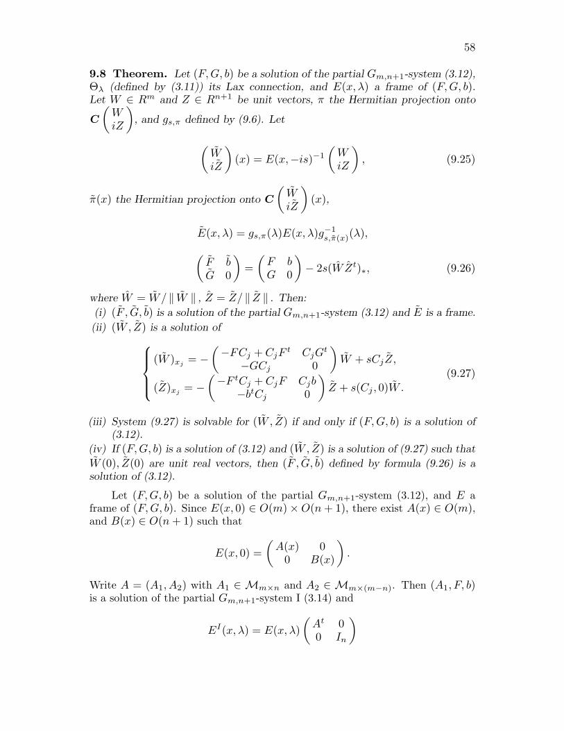
58
9.8 Theorem. Let (F, G, b) be a solution of the partial Gm,n+1-system (3.12),Θλ (defined by (3.11)) its Lax connection, and E(x, λ) a frame of (F, G, b).Let W ∈ Rm and Z ∈ Rn+1 be unit vectors, π the Hermitian projection onto
C
(WiZ
), and gs,π defined by (9.6). Let
(WiZ
)(x) = E(x,−is)−1
(WiZ
), (9.25)
π(x) the Hermitian projection onto C
(WiZ
)(x),
E(x, λ) = gs,π(λ)E(x, λ)g−1s,π(x)(λ),
(F bG 0
)=
(F bG 0
)− 2s(W Zt)∗, (9.26)
where W = W/ ‖ W ‖ , Z = Z/ ‖ Z ‖ . Then:
(i) (F , G, b) is a solution of the partial Gm,n+1-system (3.12) and E is a frame.
(ii) (W , Z) is a solution of
(W )xj = −(−FCj + CjF
t CjGt
−GCj 0
)W + sCjZ,
(Z)xj = −(−F tCj + CjF Cjb
−btCj 0
)Z + s(Cj , 0)W .
(9.27)
(iii) System (9.27) is solvable for (W , Z) if and only if (F, G, b) is a solution of(3.12).
(iv) If (F, G, b) is a solution of (3.12) and (W , Z) is a solution of (9.27) such that
W (0), Z(0) are unit real vectors, then (F , G, b) defined by formula (9.26) is asolution of (3.12).
Let (F, G, b) be a solution of the partial Gm,n+1-system (3.12), and E aframe of (F, G, b). Since E(x, 0) ∈ O(m) × O(n + 1), there exist A(x) ∈ O(m),and B(x) ∈ O(n + 1) such that
E(x, 0) =(
A(x) 00 B(x)
).
Write A = (A1, A2) with A1 ∈ Mm×n and A2 ∈ Mm×(m−n). Then (A1, F, b)is a solution of the partial Gm,n+1-system I (3.14) and
EI(x, λ) = E(x, λ)(
At 00 In
)
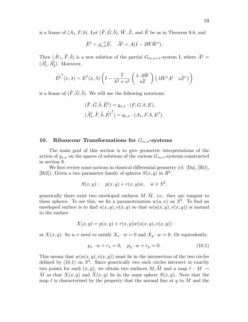
59
is a frame of (A1, F, b). Let (F , G, b), W , Z, and E be as in Theorem 9.8, and
E% = g−1s,πE, A% = A(I − 2WW t).
Then (A%1, F , b) is a new solution of the partial Gm,n+1-system I, where A% =
(A%1, A
%2). Moreover,
E%I(x, λ) = EI(x, λ)
(I − 2
λ2 + s2
(λ AW
sZ
) (λW tAt sZt
))
is a frame of (F , G, b). We will use the following notations:
(F , G, b, E%) = gs,π · (F, G, b, E),
(A%1, F , b, E%
I) = gs,π · (A1, F, b, EI).
10. Ribaucour Transformations for Gm,n-systems
The main goal of this section is to give geometric interpretations of theaction of gs,π on the spaces of solutions of the various Gm,n-systems constructedin section 9.
We first review some notions in classical differential geometry (cf. [Da], [Bi1],[Bi2]). Given a two parameter family of spheres S(x, y) in R3,
S(x, y) : p(x, y) + r(x, y)w, w ∈ S2,
generically there exist two enveloped surfaces M, M , i.e., they are tangent tothese spheres. To see this, we fix a parametrization w(u, v) on S2. To find anenveloped surface is to find u(x, y), v(x, y) so that w(u(x, y), v(x, y)) is normalto the surface
X(x, y) = p(x, y) + r(x, y)w(u(x, y), v(x, y))
at X(x, y). So u, v need to satisfy Xx · w = 0 and Xy · w = 0. Or equivalently,
px · w + rx = 0, py · w + ry = 0. (10.1)
This means that w(u(x, y), v(x, y)) must lie in the intersection of the two circlesdefined by (10.1) on S2. Since generically two such circles intersect at exactlytwo points for each (x, y), we obtain two surfaces M, M and a map . : M →M so that X(x, y) and X(x, y) lie in the same sphere S(x, y). Note that themap . is characterized by the property that the normal line at q to M and the

60
normal line at .(q) = q to M meet at equidistance r(q). We call such map .
a sphere congruence. A sphere congruence . : M → M is called a Ribaucourtransformation if it preserves line of curvature directions and the lines p + teand .(p) + t.∗(e) meet at equidistance for any principal direction e ∈ TMp andp ∈ M .
Natural generalizations of sphere congruence and Ribaucour transformationto submanifolds in space forms are given in [DT]. For x ∈ Nm(c) and v ∈TNm(c)x, let γx,v(t) = exp(tv) denote the geodesic.
10.1 Definition ([DT]). Let Mn and Mn be submanifolds of the space formNm(c). A sphere congruence is a vector bundle isomorphism P : ν(M) → ν(M)that covers a diffeomorphism . : M → M with the following properties:(a) If ξ is a parallel normal vector field of M , then P ξ.−1 is a parallel normal
field of M .(b) For any nonzero vector ξ ∈ νx(M), the geodesics γx,ξ and γ(x),P (ξ) intersect
at a point that is equidistant from x and .(x) (the distance depends on x).
10.2 Definition ([DT]). A sphere congruence P : ν(M) → ν(M) that covers. : M → M is called a Ribaucour Transformation if it satisfies the followingadditional properties:(i) If e is an eigenvector of the shape operator Aξ of M , then .∗(e) is an eigen-
vector of the shape operator AP (ξ) of M .(ii) the geodesics γx,e and γ(x),∗(e) intersect at a point equidistant to x and
.(x).
Below we show that the action of gs,π on solutions of the Gm,n-system Icorrespond to a Ribaucour transformation for flat submanifolds in Sn+m−1.
10.3 Theorem. Let EI be a frame of the solution (A1, F ) of the Gm,n-systemI (3.4), gs,π given by (9.6), and
(A%1, F , E%
I) = gs,π · (A1, F, EI)
as in section 9. Write
EI(x, 1) = (X(x), en+2(x), · · · , en+m(x), e1(x), · · · , en(x)),
E%I(x, 1) = (X(x), en+2(x), · · · , en+m(x), e1(x), · · · , en(x)).
(10.2)
Then:(1) Both X and X are immersions of flat n-dimensional submanifolds of Sn+m−1
with flat, non-degenerate normal bundle, x1, · · · , xn line of curvature coor-dinates, eαn+m
α=n+2 and eαn+mα=n+2 are parallel normal frames for X and
X respectively.

61
(2) (A1, F ) and (A%1, F ) are solutions of (3.4) corresponding to X and X as in
Theorem 6.1 respectively.(3) The bundle morphism P : ν(M) → ν(M) defined by P (eα(x)) = eα(x) forn + 2 ≤ α = n + m is a Ribaucour Transformation covering the map X(x) $→X(x).
PROOF.(1) and (2) follow from Theorems 6.1 and 9.3.
(3) Let A2, G and A = (A1, A2) be given as in Proposition 3.6, and W , Zas in Theorem 9.3. Let
γ = (γn+1, . . . , γm+n, γ1, . . . , γn) =(sin ρ W tAt cos ρ Zt
),
where sin ρ = 1/√
1 + s2 and cos ρ = s/√
1 + s2. Substitute λ = 1 in (9.23) toget
E%I(x, 1) = EI(x, 1)
(I − 2
(sin ρ AWcos ρ Z
) (sin ρ W tAt cos ρ Zt
)). (10.3)
Substitute (10.2) to the above equation to get formulas for each column of E'I:
X = X(1 − 2γ2n+1) − 2γn+1
m∑
j=2
γn+jen+j +n∑
j=1
γjej
,
ei = −2γn+1γiX − 2γi
m∑
j=2
γn+jen+j +m∑
j=1
γjej
+ ei,
en+i = −2γn+1γn+iX − 2γn+i
m∑
j=2
γn+jen+j +m∑
j=1
γjej
+ en+i.
So we haveγiX − γn+1ei = γiX − γn+1ei,
γn+iX − γn+1ei = γn+iX − γn+1ei.
Letψi = arctan(γn+1/γi), and φi = arctan(γn+1/γn+i).
Then the above equations are
cos ψi X − sinψi ei = cos ψi X − sinψi ei,
cos φiX − sinφien+i = cos φiX − sinφien+i.(10.4)

62
Geometrically, this means that the geodesic of Sn+m−1 at X(x) in the directionei(x) intersects the geodesic of Sn+m−1 at X(x) in the direction ei(x) at a pointequidistant to X(x) and X(x). So P is a Ribaucour Transformation.
Note that the distance φi and ψi’s in (10.4) in the proof of Theorem 10.3satisfy ∑n
i=1 cot2 ψi(x)1 +
∑mi=2 cot2 φi(x)
= s2,
for all x.The following theorem gives the geometric transformation for flat subman-
ifolds in Rn+m corresponding to the action of gs,π on the space of solutions ofthe Gm,n-system I. The proof is similar to that of Theorem 10.3.
10.4 Theorem. Let X be a local isometric immersion of Rn in Rn+m withflat and non-degenerate normal bundle, and (x1, · · · , xn) a line of curvature co-ordinate system. Let (A1, F ) be the corresponding solution of the Gm,n-systemI (3.4), b, g as in Theorem 6.3 (i) and (ii), and EI a frame of (A1, F ) with
EI(x, 1) = g(x). Let A, G be as in Proposition 3.6, and E = EI
(A 00 In
)
a frame for the solution ξ =(
FG
)of (3.1). Let gs,π, W , Z, W = W/ ‖ W ‖ ,
Z = Z/ ‖ Z ‖ be as in Theorem 9.3 for the solution ξ, E a frame of ξ, and
(F , G, E%) = gs,π · (F, G, E), (A%1
I
, F , E%I) = gs,π · (A1, F, EI)
as in section 9. Write
EI(x, 1) = (en+1(x), · · · , en+m(x), e1(x), · · · , en(x)),
E%I(x, 1) = (en+1(x), · · · , en+m(x), e1(x), · · · , en(x)).
Setγ = (γn+1, . . . , γm+n, γ1, . . . , γn) :=
(sin ρ W tAt cos ρZt
),
η(x) = EI(x, 1)γ(x)t, where ρ = cot−1 s.
Then:(1) There exists φ such that φxi
= −sbizi for all i = 1, . . . , n, where zi is the
i-th coordinate of Z.(2) Let X = X + 2 cos ρ φ
||W || η. Then X is again an immersed flat submanifold in
Rn+m with flat and non-degenerate normal bundle.(3) The bundle morphism P (eα(x)) = eα(x) for n + 1 ≤ α ≤ n + m is a
Ribaucour Transformation covering the map X(x) $→ X(x).
(4) The solution of (3.4) corresponding to X is (A%1, F ).

63
PROOF.(1) By (9.19), we have (zj)xi
= fij zj . Theorem 6.3 implies that (bi)xj=
fijbj for i = j. A direct computation gives (bizi)xj = (bj zj)xi . So φ exists.(2) It follows from the definition of η and equation (9.19) for wi, zj that
dη = −s
(n∑
i=1
ziwidxi
)η +
s
cos ρ
n∑i=1
widxiei
and
d
(1
||W ||
)= − s
||W ||
(n∑
i=1
ziwidxi
).
A straightforward calculation gives
dX = dX +2 cos ρ
sd
(φ
||W ||η
)=
∑i
bidxiei,
where bi = bi + 2φwi
||W || . Hence X is a submanifold with the stated properties.
(3) Set λ = 1 in equation (9.23) to get
ei = ei − 2γiη.
So we haveX +
cos ρφ
γis||W ||ei = X +
cos ρφ
γis||W ||ei,
which implies that P is a Ribaucour Transformation covering X $→ X.(4) follows from (2) and (3).
The following theorem gives the geometric transformation for local isometricimmersions of Sn in Sm+n corresponding to the action of gs,π on the space ofsolutions of the partial Gm,n+1-system I.
10.5 Theorem. Let X be a local isometric immersion of Sn in Sn+m with flatand non-degenerate normal bundle, and (x1, · · · , xn) a line of curvature coordi-nate system. Let (A1, F, b) be the solution of the partial Gm,n+1-system I (3.14)corresponding to X,
g = (en+1, · · · , en+m, e1, · · · , en, X)
as in Theorem 6.5, EI the frame of (A1, F, b) such that EI(x, 1) = g(x), and
(A%1, F , b, E%
I) = gs,π · (A1, F, b, EI)

64
as in section 9. Write
E%I(x, λ) = (en+1(x), · · · , en+m(x), e1(x), · · · , en(x), X(x)).
Then:(i) X is a local isometric immersion of Sn in Sn+m with flat and non-degenerate
normal bundle, x is line of curvature coordinates, and eαn+mα=n+1 is a parallel
normal frame.
(ii) The solution of (3.14) corresponding to X is (A%1, F , b).
(iii) The bundle morphism P (eα(x)) = eα(x) for n + 1 ≤ α ≤ n + m is a
Ribaucour Transformation that covers the map X(x) $→ X(x).
Next we give the geometric transformation for n-tuples in Rm of type O(n)corresponding to the action of gs,π on the space of solutions of the Gm,n-systemII.
10.6 Theorem. Let ξ =(
FG
)be a solution of the Gm,n-system (3.1), E a
frame of ξ, E(x, 0) =(
A(x) 00 B(x)
), (F, G, B) the corresponding solution of
the Gm,n-system II (3.10), and
(F , G, B%, E%II
) = gs,π · (F, G, B, EII), A% = gs,π · A.
Let ei and ei denote the i-th columns of A and A% respectively. Then:(i)
∂E
∂λ(x, 0)E−1(x, 0) =
(0 X(x)
−X(x)t 0
),
∂E%
∂λ(x, 0)E%
−1(x, 0) =
(0 X(x)
−Xt(x) 0
)
for some X and X.(ii) X = (X1, · · · , Xn) and X = (X1, · · · , Xn) are n-tuples in Rm of type O(n)
such that eαmα=n+1 and eαm
α=n+1 are parallel normal frame for Xj and
Xj respectively for all 1 ≤ j ≤ n.
(iii) The solutions of the Gm,n-system II (3.10) corresponding to X and X as
given in Theorem 6.8 are (F, G, B) and (F , G, B%) respectively.(iv) The bundle morphism P (eα(x)) = eα(x) for n + 1 ≤ α ≤ m is a Ribaucour
Transformation covering the map Xj(x) $→ Xj(x) for each 1 ≤ j ≤ n.
(v) There exist maps φij such that Xj + φijei = Xj + φij ei for 1 ≤ j ≤ n and1 ≤ i ≤ m.

65
PROOF. It follows from Theorem 6.8, Proposition 6.10, Corollary 6.11 andformula (9.21) that
(0 X
−Xt 0
)=
∂E%
∂λ(x, 0)E%
−1(x, 0)
=∂E
∂λ(x, 0)E(x, 0)−1 +
2sE(x, 0)
(0 W Zt
−ZW t 0
)E(x, 0)−1
=∂E
∂λ(x, 0)E(x, 0)−1 +
2s
(0 AWZtB−1
−BZW tA−1 0
)
=(
0 X−Xt 0
)+
2s
(0 AWZtB−1
−BZW tA−1 0
).
SoX = X +
2sAW ZtBt.
Let η =∑m
j=1 wjej . Then
Xi = Xi +2s
n∑j=1
zjbji η.
By (9.22), we get ei = ei − 2wiη. Hence for each 1 ≤ l ≤ m and 1 ≤ i ≤ n wehave
Xj + φijei = Xj + φij ei, where φij =∑n
l=1 zlblj
swi.
This finishes the proof.
10.7 Example. Recall that when n = 2 and m = 3, the G3,2- system II (3.10)is (6.13), which is the Gauss-Codazzi equation for surfaces in R3 parametrizedby spherical line of curvature coordinates. Let (u, r1, r2) be a solution of (6.13),and (F, G, B) defined by (6.14) the corresponding solution of (3.10). Let W , Z
as in Theorem 9.3 for the solution ξ =(
FG
)and E a frame, and (F , G, B%) =
gs,π · (F, G, B). Then
F =(
0 ux
−uy 0
), G = (r1, r2), B% =
(cos u sin usin u − cos u
)
for some solution (u, r1, r2) of (6.13). To see this, we write
Zt = (z1, z2) = (− sinα, cos α)

66
for some function α. It follows from (9.22) that
B% = B(I − 2ZZt) =(
cos u sinu− sinu cos u
) (cos 2α sin 2αsin 2α − cos 2α
)
=(
cos(−u + 2α) sin(−u + 2α)sin(−u + 2α) − cos(−u + 2α)
).
Let X = (X1, X2) and X = (X1, X2) be the 2-tuples in R2 of type O(2) cor-responding to (F, G, B) and (F , G, B%) as in Theorem 10.6. Then the first andsecond fundamental forms of X1 and X2 are given by
I1 = cos2(−u + 2α)dx2 + sin2(−u + 2α)dy2,
II1 = −r1 cos(−u + 2α)dx2 − r2 sin(−u + 2α)dy2,
I2 = sin2(−u + 2α)dx2 + cos2(−u + 2α)dy2,
II2 = −r1 sin(−u + 2α)dx2 + r2 cos(−u + 2α)dy2, where
ri = ri − 2sw3zi = ri −2sw3zi
z21 + z2
1
.
10.8 Example. Let (u, r1, r2) = (0, 0, 0) be the trivial solution of (6.13). Itis easy to see that the 2-tuple in R3 of type O(2) corresponding to the trivialsolution is
X =
(−x 00 −y0 0
)
and
E(x, y, λ) =
cos λx 0 0 − sinλx 00 cos λy 0 0 − sinλy0 0 1 0 0
sinλx 0 0 cos λx 00 sinλy 0 0 cos λy
is a frame for the trivial solution.Below we write down explicitly the 2-tuple in R3 of type O(2) constructed
by applying the Ribaucour transformation to the trivial solution. It follows fromTheorems 10.6 (i) and 9.3 that
w1
w2
w3
z1
z2
=
cosh(sx)w1 + sinh(sx)z1
cosh(sy)w2 + sinh(sy)z2
w3
cosh(sx)z1 + sinh(sx)w1
cosh(sy)z2 + sinh(sy)w2
. (10.5)
Use Theorem 10.6 and a direct computation to get:

67
(i) If |z1| ≥ |w1| and |z2| ≥ |w2|, then
X1 = −(
x00
)+
2a cosh(sx)s(a2 cosh2(sx) + b2 cosh2(sy))
(a sinh(sx)b sinh(sy)
w3
),
X2 = −(
x00
)+
2b cosh(sy)s(a2 cosh2(sx) + b2 cosh2(sy))
(a sinh(sx)b sinh(sy)
w3
),
where a =√
z21 − w2
1, b =√
z22 − w2
2, and a2 + b2 = w23 < 1. See Figure 1.
(ii) If |w1| ≥ |z1| and |z2| ≥ |w2|, then
X1 = −(
x00
)+
2a sinh(sx)s(a2 sinh2(sx) + b2 cosh2(sy))
(a cosh(sx)b sinh(sy)
w3
),
X2 = −(
x00
)+
2b cosh(sy)s(a2 sinh2(sx) + b2 cosh2(sy))
(a cosh(sx)b sinh(sy)
w3
),
where a =√
w21 − z2
1 , b =√
z22 − w2
2, and 0 ≤ b2 − a2 = w23 < 1. See
Figure 2.
(iii) The first and second fundamental forms of X1 are
I1 = cos2(2α)dx2 + sin2(2α)dy2,
II1 = −2sw3
τsin(α) cos(2α)dx2 +
2sw3
τcos(α) sin(2α)dy2,
where z1, z2 are given by (10.5), tanα = −z1/z2, and
τ = (cosh(sx)z1 − sinh(sx)w1)2 + (cosh(sy)z2 − sinh(sy)w2)212 .
We have seen in Example 6.16 that(i) solutions of SGE correspond to K = −1 surfaces of R3 up to rigid motion,(ii) (u, sinu,− cos u) is a solution of (6.13) if and only if u is a solution of the
SGE,(iii) if (X1, X2) is the 2-tuple corresponding to (u, sinu,− cos u), then X1 has
Gaussian curvature −1, u is the corresponding solution of the SGE, and X2
is the unit normal of X1.
Below we give a condition on s, π so that the action of gs,π on (X, e3) alsorepresents a 2-tuple in R3 of type O(2) corresponding to a K = −1 surface.

68
10.9 Corollary. Let (u, sinu,− cos u) be a solution of (6.13), Z = (z1, z2)t,W = (w1, w2, w3)t real constant unit vectors, and constant s such that
sw3 = z1 sinu(0, 0) − z2 cos u(0, 0).
Let π denote the Hermitian projection onto (w1, w2, w3, iz1, iz2)t. Then the newsolution gs,π · (u, sin u,− cos u) of (6.13) is of the form (u, sin u,− cos u) for someu.
PROOF. Let Z, W , Z, W be as in Theorem 9.3 for the solution ξ =(
FG
)of the G3,2-system, where F and G are defined by (6.14). Since (W , Z) satisfies(9.19), we have
dw3 = sinu w1dx1 − cos u w2dx2,dz1 = −z1du + sw1dx1,dz2 = z1du + sw2dx2.
Thus sdw3 = sinu (dz1 + z2du)− cos u (dz2 − z1du) = d(sinu z1 − cos u z2). Itfollows that sw3 = sinuz1 − cos uz2.
10.10 Example. u = 0 is the trivial solution of the SGE. It follows fromExample 6.16 that (0, 0,−1) is a solution of (6.13). Use Corollary 10.9 andExample 10.7 to compute gs,π·(0, 0,−1) to get three parameter family of solutionsof the SGE. Some of these examples (see Figure 3) are:
(1) If 0 < s = sin c ≤ 1, then
u = 2 tan−1
(sin c sin(y cos c)
cos c cosh(x sin c)
). (10.6)
This is the breather solution for the SGE, and the corresponding curvature−1 surface in R3 is given by
X = −(
x00
)+ r
( sinh(x sin c)cos y cos(y cos c) + secc sin y sin(y cos c)sin y cos(y cos c) − secc cos y sin(y cos c)
),
where
r =2 cosh(x sin c)
sin ccosh2(x sin c) + tan2 c sin2(y cos c).
(2) If s = cosh c > 1, then
u = 2 tan−1
(cosh c cosh(y sinh c)sinh c sinh(x cosh c)
),
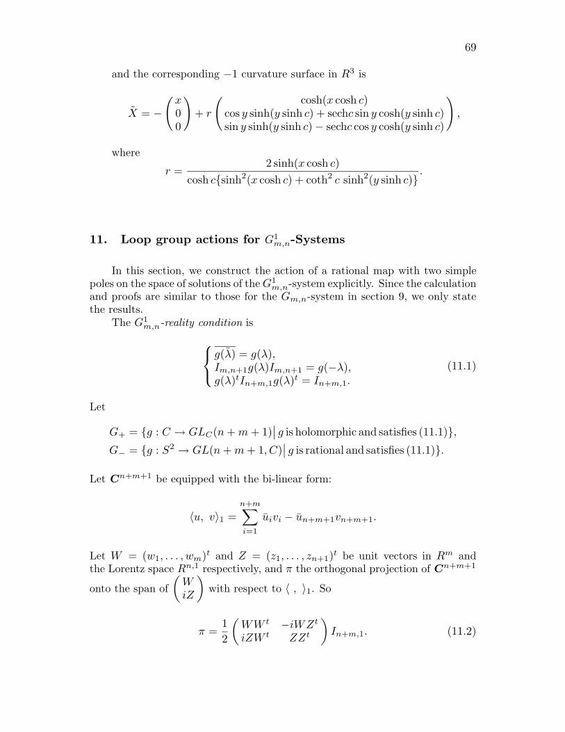
69
and the corresponding −1 curvature surface in R3 is
X = −(
x00
)+ r
( cosh(x cosh c)cos y sinh(y sinh c) + sechc sin y cosh(y sinh c)sin y sinh(y sinh c) − sechc cos y cosh(y sinh c)
),
where
r =2 sinh(x cosh c)
cosh csinh2(x cosh c) + coth2 c sinh2(y sinh c).
11. Loop group actions for G1m,n-Systems
In this section, we construct the action of a rational map with two simplepoles on the space of solutions of the G1
m,n-system explicitly. Since the calculationand proofs are similar to those for the Gm,n-system in section 9, we only statethe results.
The G1m,n-reality condition is
g(λ) = g(λ),Im,n+1g(λ)Im,n+1 = g(−λ),g(λ)tIn+m,1g(λ)t = In+m,1.
(11.1)
Let
G+ = g : C → GLC(n + m + 1)∣∣ g is holomorphic and satisfies (11.1),
G− = g : S2 → GL(n + m + 1, C)∣∣ g is rational and satisfies (11.1).
Let Cn+m+1 be equipped with the bi-linear form:
〈u, v〉1 =n+m∑i=1
uivi − un+m+1vn+m+1.
Let W = (w1, . . . , wm)t and Z = (z1, . . . , zn+1)t be unit vectors in Rm andthe Lorentz space Rn,1 respectively, and π the orthogonal projection of Cn+m+1
onto the span of(
WiZ
)with respect to 〈 , 〉1. So
π =12
(WW t −iWZt
iZW t ZZt
)In+m,1. (11.2)

70
Since Z, W are real vectors, ππ = ππ = 0. Given non-zero s ∈ R, define
qs,π(λ) =(
π +λ − is
λ + is(I − π)
) (π +
λ + is
λ − is(I − π)
)=
1λ2 + s2
(λ2I + 2sλ
(0 WZtJ
−ZW t 0
)+ s2
(I − 2WW t 0
0 I − 2ZZtJ
)),
(11.3)where J = In,1 = diag(1, · · · , 1,−1). A direct computation implies that qs,π
satisfies the reality condition (11.1). So qs,π ∈ G−.
11.1 Theorem. Let ξ be a solution of the G1m,n-system (4.2), θλ its Lax con-
nection as in (4.1), and E a frame for ξ. Let W and Z be unit vectors in Rm
and Rn,1, (WiZ
)(x) = E(x,−is)−1
(WiZ
), (11.4)
and π(x) the orthogonal projection onto the span of
(WiZ
)(x) with respect to
〈 , 〉1. Let 0 = s ∈ R be a constant, π a projection onto C
(WiZ
), and qs,π
defined by (11.3). Set
E(x, λ) = qs,π(λ)E(x, λ)q−1s,π(x)(λ),
ξ = ξ − 2s(W ZtJ)∗,
where W (x) = 1||W (x)||m
W (x) and Z(x) = 1||Z(x)||n,1
Z(x), and (y∗)ij = yij for
i = j and (y∗)ii = 0 for all i. Let
E%(x, λ) = E(x, λ)q−1s,π(x)(λ).
Then(i) ξ is a new solution of (4.2),
(ii) E% is a frame for ξ,
(iii) E(x, 0) =(
A(x) 00 B(x)
)and E%(x, 0) =
(A%(x) 0
0 B%(x)
)for some
A, B, A%, B%, and A% = A(I − 2WW t),B% = B(I − 2ZZt)In,1.
(11.5)
When m = n, Theorem 11.1 (i) was proved in [Zh].

71
Write ξ =(
FG
), F = (fij), G = (gij), F = (fij), G = (gij), and ξ =(
FG
). Then formula for ξ in the above theorem is
fij = fij − 2swizjεj ,gij = gij − 2swn+1+izjεj ,
(11.6)
where εj = 1 for 1 ≤ j ≤ n and εn+1 = −1.
Differentiate (11.4) to get the ODE for (W , Z):
11.2 Corollary. Let ξ =(
FG
)be a solution of the G1
m,n-system (4.2), E a
frame of ξ, and (W , Z) be as in Theorem 11.1. Then (W , Z) is a solution of thefollowing system
(wi)xi = −∑n+1
j =i fjiwj −∑m−n−1
j=1 gjiwj+n+1 + sziεi, i ≤ n + 1(wi)xj
= fijwj , i ≤ n + 1, j = i,(wi)xj = gijwj , i > n + 1,(zi)xj = fjizjεiεj , j = i,
(zi)xi = −∑n+1
j =i fij zj + swi.
(11.7)
11.3 Corollary. Let ξ =(
FG
)be a solution of the G1
m,n-system (4.2). Then
system (11.7) is always solvable. Moreover, if (W , Z) is a solution of (11.7) such
that W (0) and Z(0) are unit vectors in Rm and Rn,1 respectively, then
(FG
)is
a solution of (4.2), where F and G are defined by (11.6).
WriteA = (A1, A2), A% = (A%
1, A%2)
with A1, A%1 ∈ Mm×(n+1) and A2, A
%2 ∈ Mm×(m−n−1). Then (A1, F ) and
(A%1, F ) are solutions of the G1
m,n-system I (4.4), and (F, G, B) and (F , G, B%)are solutions of the G1
m,n-system II (4.6), and their frames are related by
E%(x, λ) = E(x, λ)qs,π(x)(λ)−1,
E%I(x, λ) = EI(x, λ)
(I − 2
λ2 + s2
(λAWsZ
) (λW tAt sZtJ
)),
E%II
(x, λ) = EII(x, λ)(
I − 2λ2 + s2
(s2WW t −sλW ZtBtJ
−sλBZW t λ2BZZtBtJ
)).
For the partial G1m,n-system we have

72
11.4 Theorem. Let (F, G, b) : Rn → gl∗(n)×M(m−n)×n ×Mn×1 be a solu-
tion of the partial G1m,n-system (4.8), τλ its Lax connection as in (4.7), and E a
frame for (F, G, b). Let W and Z be unit vectors in Rm and Rn,1 respectively,
(WiZ
)(x) = E(x,−is)−1
(WiZ
),
and π(x) the orthogonal projection onto the span of
(WiZ
)(x) with respect to
the bilinear form 〈 , 〉1. Let 0 = s ∈ R be a real number, π the projection onto
C
(WiZ
), and qs,π as defined in (11.3). Let
E(x, λ) = qs,π(λ)E(x, λ)q−1s,π(x)(λ),
fij = fij − 2swizj ,gij = gij − 2swn+izj ,
bi = bi + 2swizn+1,
(11.8)
where W = 1||W ||m
W , Z = 1||Z||n,1
Z and wi and zi are the i-th coordinate of
W , Z respectively. Then (F , G, b) is a solution of (4.8) and E is its frame, where
F = (fij), G = (gij), and b = (bi).
11.5 Corollary. Let ( F, G, b ) be a solution of the partial G1m,n-system (4.8),
E a frame of (F, G, b), and
(WiZ
)as in Theorem 11.4. Then (W , Z) is a solution
of
(wi)xi = −∑n
j =i fjiwj −∑m−n
j=1 gjiwj+n + szi i ≤ n ,
(wi)xj= fijwj i ≤ n, j = i ,
(wi)xj= gijwj i > n ,
(zi)xj = fjizj j = i , i ≤ n(zi)xi = −
∑nj =i fij zj − bizn+1 + swi,
(zn+1)xj = −bj zj .
(11.9)
Conversely, if (F, G, b) is a solution of system (4.8), then system (11.9) is solvable.
Moreover, if (W , Z) is a solution of (11.9) such that W (0) and Z(0) are unit
vectors in Rm and Rn,1 respectively, then (F , G, b) is also a solution of (4.8),
where F , G, b are defined by formula (11.8).
LetE%(x, λ) = E(x, λ)q−1
s,π(x)(λ).

73
Then E% is also a frame of (F , G, b). Write
E(x, 0) =(
A 00 B
)∈ O(m) × O(n, 1), E%(x, 0) =
(A%(x) 0
0 B%(x)
).
Then A% = A(I − 2WW t),B% = B(I − 2ZZtJ),
where J = In,1.Let
EI(x, λ) = E(x, λ)(
At 00 In+1
), E%
I(x, λ) = E(x, λ)
(At 00 In+1
).
A direct computation gives
E%I(x, λ) = EI(x, λ)
(I − 2
λ2 + s2
(λAWsZ
) (λW tAt sZtJ
)).
Note that EI and E%I
are frames of (A1, F, b) and (A%1, F , b) respectively. We
use the same type of notations as in previous sections:
(F , G, b, E%) = qs,π · (F, G, b, E),
(A%1
,
F , b, E%I) = qs,π · (A1, F, b, E),
(A%, B%) = qs,π · (A, B).
12. Ribaucour Transformations for G1m,n-Systems
In this section, we describe the corresponding geometric transformations onsubmanifolds associated to the action of qs,π on the space of solutions of variousG1
m,n-systems described in section 11.
12.1 Theorem. Let X be a local isometric immersion of Hn in Hn+m with flatand non-degenerate normal bundle, (x1, . . . , xn) line of curvature coordinates,and (A1, F, b) the solution of the G1
m,n-system I (4.10) corresponding to X as
defined in Theorem 7.3. Let EI(x, λ) be a frame of (A1, F, b), and g(x) =
EI(x, 1). Let 0 = s ∈ R, π the projection onto C
(WiZ
), qs,π defined by (11.3),
and E%I, A%
i as in section 11. Write
(A%1, F , b, E%
I) = qs,π · (A1, F, b, EI),
EI(x, 1) = (en+1(x), · · · , en+m(x), e1(x), · · · , en(x), X(x)),
E%I(x, 1) = (en+1(x), · · · , en+m(x), e1(x), · · · , en(x), X(x)).

74
Then:(i) X is a local isometric immersion of Hn in Hn+m with non-degenerate, flat
normal bundle, and eαn+mα=n+1 is a parallel normal frame.
(ii) The solution of (4.10) corresponding to X given in Theorem 7.3 is (A%1, F , b).
(iii) The bundle morphism P (eα(x)) = eα(x) for n + 1 ≤ α ≤ n + m is a
Ribaucour transformation covering the map X(x) $→ X(x).
Recall that if v0 is a null vector in R2n,1 and c = 0, then by Proposition 7.1that
Nv0,c = x ∈2n,1 | 〈x, x〉1 = −1, 〈x, v0〉1 = cis a totally umbilic hypersurface of H2n, and Nv0,c is isometric to R2n−1. Nextwe give a condition on s, π so that the Ribaucour transformation correspondingto qs,π for local isometric immersions of Hn in H2n preserves local isometricimmersions of Hn in R2n−1.
12.2 Corollary. Let v0 be a null vector in R2n,1, X a local isometric immersionof Hn in Nv0,c ⊂ H2n with flat and non-degenerate normal bundle, and W, Z,
qs,π and X as in Theorem 12.1. If
bt(0)W = −szn+1,
then X also lies in some flat totally umbilic hypersurface of H2n.
PROOF. By Theorem 7.3 (vi), there exists some constant vector w ∈ Mn×1
such that b = Atw. It follows from 2.4 thatdw = −
∑(−FCi + CiF
t)wdxi + s∑
ziCidxi,dzn+1 = −
∑bizidxi.
Since AtdA =∑
(−FCi + CiFt)dxi, we have
d(btW ) = wtd(AW ) = wt(dA)W + wtAdW = bt(s∑
ziCidxi) = −sdzn+1.
Hence btW = −szn+1 for all x ∈ Rn.A straightforward calculation now impliesthat
A%tw = A(I − 2WW t)Atw = b + 2szn+1W = b,
which finishes the proof.
12.3 Theorem. Let (F, G, B) be a solution of the G1m,n-system II (4.6), and
X = (X1, · · · , Xn+1) the (n+1)-tuple in Rm of type O(n, 1) corresponding to(F, G, B) of (4.6) as described in Theorem 7.4. Let qs,π be the rational mapdefined by (11.3) for some constant s and unit vectors W in Rm and Z in Rn,1,and
(F , G, B%, A%) = qs,π · (F, G, B, A).

75
Let
X = X +2sAW ZtBtJ = (X1, · · · , Xn+1), (12.1)
where J = In,1. Then:
(i) X is a (n+1)-tuple in Rm of type O(n, 1).(ii) The solution of (4.6) corresponding to X is (F , G, B%) = qs,π · (F, G, B).(iii) Write A = (e1, · · · , em), A% = (e1, · · · , em). Then ein
i=1 and eini=1
are principal curvature frames, and eαmα=n+1 and eαm
α=n+1 are parallel
normal frames of Xj and Xj respectively.
(iv) The bundle morphism P (eα(x)) = eα(x) for n + 2 ≤ α ≤ m is a Ribaucour
transformation covering the map Xj(x) $→ Xj(x) for each 1 ≤ j ≤ n.
(v) There exist smooth functions φij such that
Xj + φijei = Xj + φij ei (12.2)
for all 1 ≤ j ≤ n and 1 ≤ i ≤ n.
13. Darboux Transformations for G1m,1-Systems
Let M, M be two surfaces in Rm with flat and non-degenerate normal bun-dle, and P : ν(M) → ν(M) a Ribaucour transformation that covers . : M → M .If in addition . is a conformal diffeomorphism, then P is called a Darboux trans-formation. Such transformations for surfaces in R3 were studied by Darbouxand Bianchi and in Rm by Burstall [Bu]. In this section, we show that the trans-formation constructed in Theorem 12.3 for 2-tuples in R3 of type O(1, 1) is aDarboux transformation for isothermic surfaces.
13.1 Theorem. Let (Y1, Y2) be an isothermic pair in Rm corresponding to the
solution (u, G) of (8.2), and ξ =(
FG
)the corresponding solution of the G1
m,1-
system, where F =(
0 ux
uy 0
). Let 0 = s ∈ R, π the projection onto C
(WiZ
),
qs,π the rational map defined by (11.3), and W , Z as in Theorem 11.1 for the
solution ξ =(
FG
)of the G1
m,1-system. Let
B =(
cosh u sinhusinhu cosh u
), (E%
II, A%, B%) = qs,π · (EII , A, B).

76
Write A = (e1, · · · , em) and A% = (e1, · · · , em). Set
Y1 = Y1 +2s(z1 + z2)eu
m∑i=1
wiei,
Y2 = Y2 +2s(z1 − z2)e−u
m∑i=1
wiei.
(13.1)
Then(i) (Y1, Y2) is an isothermic pair,
(ii) (u, G) is the solution of (8.2) corresponding to (Y1, Y2), where u = 2α − u,
sinhα = −z2 and G = (gij) is defined by (11.6),
(iii) the fundamental forms of (Y1, Y2) are
I1 = e−2u(dx2 + dy2),II1 = e−u
∑m−2j=1 (gj1dx2 − gj2dy2)e2+j ,
I2 = e2u(dx2 + dy2),II2 = eu
∑m−2j=1 (gj1dx2 + gj2dy2)ej+2,
(iv) the bundle morphism P (eα(x)) = eα(x) for 3 ≤ α ≤ m covering Yi $→ Yi isa Darboux transformation for each 1 ≤ i ≤ 2.
PROOF. Let X1 = (Y1 + Y2)/2, and X2 = (Y2 − Y1)/2. By Propositions8.1, 8.5 and 8.6, (F, G, B) is a solution of the G1
m,1-system II, and X = (X1, X2)is the corresponding 2-tuples in Rm of type O(1, 1). Let X = (X1, X2) be as inTheorem 12.3, and
Y1 = X1 − X2, Y2 = X1 + X2.
It follows from (12.1) that Y1, Y2 are given by (13.1).Since z2
1 − z22 = 1, there exists a function α : R2 → R such that
z1 = cosh α, z2 = − sinhα.
Since u = 2α − u,
e−u = eu z1 + z2
z1 − z2. (13.2)
Use (11.5), (13.2) and a direct computation to get
B% = B(I − 2ZZtJ) =(− cosh(2α − u) − sinh(2α − u)sinh(2α − u) cosh(2α − u)
)
=(− cosh u − sinh usinh u cosh u
).
(13.3)

77
So (i)-(iii) follows.To prove (iv), we first note that the map Yi $→ Yi is conformal because
(x, y) are isothermic coordinates for Yi and Yi. It remains to prove that P is aRibaucour transform. To see this, we use (12.2) to get
Y1 + (φi1 − φi2)ei = Y1 + (φi1 − φi2)ei,
Y2 + (φi1 + φi2)ei = Y2 + (φi1 + φi2)ei
for each 1 ≤ i ≤ m. So P is a Darboux transformation.
Let (Y1, Y2) be an isothermic pair in R3 corresponding to the solution (u, G)of (8.2), and (Y1, Y2) as in Theorem 13.1. Write G = (g1, g2)t. Then the meancurvature for Yi and Yi are given as follows:
H1 =−g1 − g2
eu
H2 =−g1 + g2
e−u
H1 =g1 − g2
e−u=
z1 − z2
eu(z1 + z2)g1 − g2 − 2sw3(z1 + z2)
H2 =g1 + g2
eu=
eu(z1 + z2)z1 − z2
g1 + g2 − 2sw3(z1 − z2).
(13.4)
13.2 Example. A plane in R3 is the isothermic surface corresponding to thetrivial solution (0, 0, 0) of (8.2). Let W = (w1, w2, w3)t, Z = (z1, z2)t be unitvectors in R3 and R1,1 respectively. Use Theorem 11.1 and a direct computationto get
w1
w2
w3
z1
z2
(x, y) =
w1 cosh sx + z1 sinh sxw2 cos sy + z2 sin sy
w3
z1 cosh sx + w1 sinh sx−w2 sin sy + z2 cos sy
.
Then the isothermic pair (Y1, Y2) corresponding to (u, g1, g2) = qs,π · (0, 0, 0) isgiven by
Y1 =
(−xy0
)+
2scosh γ cosh(sx) − cos(sy)
( cosh γ sinh(sx)sin(sy)− sinh γ
),
Y2 =
(−x−y0
)+
2scosh γ cosh(sx) + cos(sy)
( cosh γ sinh(sx)sin(sy)− sinh γ
),

78
where cosh γ =√
z21−w2
1√z22+w2
2
is a constant parameter. See Figure 4.
The first and second fundamental forms of Y2 are given by I = e2u(dx2+dy2)and II = e2u(k1dx2 + k2dy2) where
eu =cosh γ cosh(sx) − cos(sy)cosh γ cosh(sx) + cos(sy)
,
k1 =2s sinh γ cosh γ cosh(sx)
(cosh γ cosh(sx) − cos(sy))2,
k2 =2s sinh γ cos(sy)
(cosh γ cosh(sx) − cos(sy))2.
Suppose Y1(x, y) is an immersion of a surface in R3 with constant meancurvature 2c and no umbilical points, and (x, y) is the canonical isothermic co-ordinates. It follows from Proposition 8.7 that (u, g1, g2) is a solution of (8.2),where
g1 = e−u + ceu, g2 = −e−u + ceu.
In particular, Y1 is isothermic. It follows from Theorem 7.4, Propositions 8.1 and8.6 that there exists an isothermic surface Y2 such that (Y1, Y2) is an isothermicpair corresponding to (u, g1, g2), and the principal curvatures of Y2 are
−1 − ce2u, −1 + ce2u.
So the mean curvature of Y2 is −2. If Y1 is minimal, then Y2 is totally umbilicwith mean curvature −2. Hence in this case, Y2 is a standard unit sphere. Infact, Y2 = e3 is the standard sphere parametrized by the isothermic coordinatesof Y1.
Below we give a condition on s, π so that the induced action of qs,π onthe space of isothermic surfaces preserves the subset of constant mean curvaturesurfaces parametrized by canonical isothermic coordinates.
13.3 Corollary. Let (Y1, Y2) be a isothermic pair in R3 such that Y1 has con-stant mean curvature 2c, no umbilical points, and is parametrized by the canon-ical isothermic coordinates. Let s = 0 be a constant, W, Z constant unit vectorsin Rm and R1,1 respectively, and Y = (Y1, Y2) = qs,π · (Y1, Y2) as in Theorem13.1. If
sw3 = ceu(0,0)(z1 + z2) + e−u(0,0)(z1 − z2),
then Y1 has constant mean curvature 2c and Y2 has mean curvature −2.
PROOF. By (11.8), we have
g1 = g1 − 2sw3z1, g2 = g2 + 2sw3z2.

79
Write z1 = cosh α and z2 = − sinhα for some function α. It follows from thedifferential equation (11.7) for W , Z that the derivative of
sw3 − ceu(z1 + z2) − e−u(z1 − z2) (13.5)
is zero. Since W (0) = W and Z(0) = Z, (13.5) is identically zero on R2. UseTheorem 13.1, formulas (13.3), (13.5), and a direct computation to prove thatthe mean curvature of Y1 and Y2 are 2c and −2 respectively.
Similar computation gives
13.4 Corollary. Let Y1 be a minimal surface without umbilic points in R3
parametrized by the canonical isothermic coordinates, and Y1 as in Corollary13.3. If sw3 = e−u(0,0)(z1 − z2), then Y1 is minimal.
13.5 Example.
Let Y1 =
( −xsin y
1 − cos y
)and Y2 =
( −x− sin y
−1 + cos y
). This pair of cylinders
(Y1, Y2) is an isothermic pair with (u, g1, g2) = (0, 0,−1) as the correspondingsolution to (8.2). Using Theorem 11.1 and putting s = sinh c, we obtain
w1
w2
w3
z1
z2
=
w1 cosh(x sinh c) + z1 sinh(x sinh c)w2 cos(y cosh c) + w3 cosh c sin(y cosh c)
−w2 sech c sin(y cosh c) + w3 cos(y cosh c)z1 cosh(x sinh c) + w1 sinh(x sinh c)
sinh c w2 sech c sin(y cosh c) − sinh c w3 cos(y cosh c)
.
Let (Y1, Y2) be the isothermic pair with constant mean curvatures correspondingto (u, g1, g2) = qs,π · (0, 0,−1). Then
Y1 =
( −xsin y
1 − cos y
)+ r1
(a sinh(x sinh c)
− cosh c cos y cos(y cosh c) − sin y sin(y cosh c)− cosh c sin y cos(y cosh c) + cos y sin(y cosh c)
),
Y2 =
( −x− sin y
−1 + cos y
)+ r2
(a sinh(x sinh c)
− cosh c cos y cos(y cosh c) − sin y sin(y cosh c)− cosh c sin y cos(y cosh c) + cos y sin(y cosh c)
),
where a = (z21 − w2
1)/(w23 + w2
2 sech2 c) 12 , and
r1 =2
sinh ca cosh(x sinh c) + sinh c sin(y cosh c) ,
r2 =2
sinh ca cosh(x sinh c) − sinh c sin(y cosh c) .

80
If a > sinh c and cosh c is a rational number n/k, then Y1, Y2 are immersedcylinder with n bubbles (see Figures 5, 6, 7).
Note that u and the principal curvatures ki,1, ki,2 of Yi are given by
eu =a cosh(x sinh c) + sinh c sin(y cosh c)a cosh(x sinh c) − sinh c sin(y cosh c)
,
k1,1 = − 2a sinh c cosh(x sinh c) sin(y cosh c)(a cosh(x sinh c) − sinh c sin(y cosh c))2
,
k1,2 =a2 cosh(x sinh c) + sinh2 c sin(y cosh c)(a cosh(x sinh c) − sinh c sin(y cosh c))2
,
k2,1 = − 2a sinh c cosh(x sinh c) sin(y cosh c)(a cosh(x sinh c) + sinh c sin(y cosh c))2
,
k2,2 = − a2 cosh(x sinh c) + sinh2 c sin(y cosh c)(a cosh(x sinh c) + sinh c sin(y cosh c))2
.
Note that H1 = 1 and H2 = −1. This does not contradict Corollary 13.3 becausethe isothermic coordinate system (x, y) is not the canonical one for the cylinderviewed as a CMC surface. The canonical isothermic coordinates are x/2, y/2.
14. Backlund transformations and loop group factorizations
Terng and Uhlenbeck ([TU2]) show that the classical Backlund transforma-tion of surfaces in R3 with constant curvature −1 corresponds to the action of arational map with only one simple pole on the space of solutions of the SGE. Inthis section, we give a generalization of this result to the Gn,n-system. We finda rational map that satisfies the Gn,n-reality condition and has only one simplepole, and show that the corresponding geometric action gives rise to a Backlundtransformation of n-dimensional submanifolds.
Backlund’s theorem is generalized by Tenenblat and Terng in [TT] to n-submanifolds in R2n−1, and by Tenenblat in [Ten] to submanifolds in S2n−1
and H2n−1. These generalizations arise naturally if we reformulate the classicalBacklund transformations in terms of orthonormal frames as follows: Note that. : M → M is a Backlund transformation with constant θ for surfaces M, M inR3, then there exist O(3)-frame eA and eA such that .(p) = p + sin θ e1(p) and
(e1, e2, e3)(.(x)) = (e1, e2, e3)(x)
( 1 0 00 cos θ − sin θ0 sin θ cos θ
)
for all x ∈ M .

81
14.1 Definition ([Ten]). Let M, M be n-dimensional submanifolds in S2n−1.A diffeomorphism . : M → M is a Backlund transformation with constant θ ifthere exist local orthonormal O(2n)-frames eA, eA of M, M respectively suchthat(i) e1 = X and e1 = X are the immersions,(i) eα2n−1
α=n+1 and eα2n−1α=n+1 are parallel normal frames for M, M respectively,
(iii)(X, en+1, · · · , e2n−1, e1, en)(.(x))
= (X, en+1, · · · , e2n−1, e1, · · · , en)(x)(
cos θ In − sin θ In
sin θ In cos θ In
)
for all x ∈ M .
14.2 Theorem ([Ten]). If . : Mn → Mn is a Backlund transformation in
S2n−1, then both M and M are flat. Moreover, if Mn is a flat submanifold ofS2n−1, then given any constant θ and a unit vector v0 ∈ TMp0 , there exists a
submanifold M of S2n−1 and a Backlund transformation . : M → M such that.(p0) = cos θ .(p0) + sin θ v0.
Next, we explain the relation between the geometric Backlund transforma-tion and the dressing action on the space of Gn,n-systems. By Theorem 6.1,the Gauss-Codazzi equations for flat n-dimensional submanifold in S2n−1 are theGn,n-system I, which is gauge equivalent to the Gn,n-system for F : Rn → gl∗(n)such that
θλ = λ
(0 −δδ 0
)+
(−Fδ + δF t 0
0 −F tδ + δF
)(14.1)
is flat for all λ ∈ C, where δ = diag(dx1, · · · , dxn). So the Gn,n-system is theequation for F :
CiF
txj
− FxjCi − CjF
txi
+ FxiCj = [CiF
t − FCi, CjFt − FCj ],
CiFxj − F txj
Ci − CjFxi + F txi
Cj = [CiF − F tCi, CjF − F tCj ],(14.2)
where Ci = eii = diag(0, · · · , 1, 0, · · · , 0) as before.Let s ∈ R be a non-zero constant, β ∈ O(n) a constant, and
ks,β(λ) =1
λ − is
(sβ λ−λ sβt
). (14.3)
Note that ks,β is holomorphic at λ = ∞, ks,π(∞) = I, and ks,β only satisfiesthe Gn,n-reality condition up to a scalar function, i.e.,
k(λ) =λ − is
λ + isk(λ), In,nk(λ)In,n = k(−λ), k(λ)tk(λ) =
λ2 + s2
(λ − is)2I,

82
where k = ks,β . So ks,β does not belong to G−. But the following is true: (i)an element of the form f(λ)I in G− lies in the center, (ii) the dressing actionof such element on the space of solutions of the Gn,n-system is trivial, and (iii)the factorization still works. In fact, if E is a frame of a solution F of the Gn,n-system (14.2), then ks,π(λ)E(x, λ) can still be factored as E(x, λ)ks,β(x) for some
functions β(x) and E(x, λ) so that E is holomorphic for λ ∈ C. Hence we get
14.3 Theorem. Let F be a solution of the Gn,n-system (14.2), E a frame ofF , s ∈ R a constant, β ∈ O(n) a constant matrix, and ks,β defined by (14.3).
Write E(x,−is) =(
η1(x) η2(x)η3(x) η4(x)
)with ηi ∈ Mn×n. Set
β = (iη4 − βη2)−1(iβη1 + η3),
E(x, λ) = ks,βE(x, λ)ks,β(x)(λ)−1,
F = F t + sβ∗,
(14.4)
where y∗ is the matrix whose ij-th entry is yij for i = j and is 0 for i = j. Then
(i) F is a solution of the Gn,n-system (14.2) and E is a frame of F ,
(ii) β is a solution ofdβ =
∑ni=1(−β(FCi − CiF
t) + (F tCi − CiF )β − sCi + sβCiβ)dxi,
ββt = I.
(14.5)
PROOF. First we prove that E(x, λ) is holomorphic in λ ∈ C. By defini-tion, E(x, λ) is holomorphic for all λ ∈ C except at λ = ±is, and has simplepoles at is and −is. A direct computation implies that the residue at −is is aconstant times (
β −iIn
iIn βt
) (η1 η2
η3 η4
) (βt iIn
−iIn β
),
which is zero by the definition of β. Similar computation shows that the residueof E(x, λ) at λ = is is also zero. Hence E(x, λ) is holomorphic in λ ∈ C.
Let θλ = E−1dE, and θλ = E−1dE. Then θλ is holomorphic for λ ∈ C. Itremains to prove that θλ is of the form (2.3) for some F . But
θλ = E−1dE = ks,βθλk−1
s,β− dks,βk−1
s,β. (14.6)
Because ks,β is holomorphic at λ = ∞ and θλ has only simple poles at λ = ∞,so is θλ. Compare coefficients of λi in (14.6) to conclude that θλ is of the form(2.3) for some F and F is given by (14.4). This proves (i).

83
Multiply (14.6) by ks,β on the right to get
θλks,β = ks,βθλ − dks,β .
Multiply the above equation by (λ − is) then compare coefficients of λi to getthe differential equation for β in (ii).
14.4 Corollary. Let F be a solution of the Gn,n-system (14.2), and E a frame
of F . Then system (14.5) is solvable for β. Moreover, if β is a solution of (14.5)
with initial condition β(0) = β, then F = F t + sβ∗ is a solution of (14.2).
Since solutions of the Gn,n-system I correspond to flat n-submanifolds inS2n−1, Theorem 14.3 and Corollary 14.4 give a method of constructing newflat n-submanifolds in S2n−1 from a given one. Geometrically, this gives thegeometric Backlund transformation constructed by Tenenblat [Ten]:
14.5 Theorem. Let F, E, ks,β , β, E, F be as in Theorem 14.3. Write E(x, 0) =(A(x) 0
0 B(x)
). Let
N(x) = EI(x, 1) = E(x, 1)(
A(x)t 00 In
),
N(x) = E%I(x, 1) = N(x)
(A 00 In
) (cos ρ βt − sin ρ In
sin ρ In cos ρ β
) (A%
t0
0 In
),
(14.7)where ρ = arctan(1/s), and A% = Aβt. Let vi and vi denote the i-th column of N
and N respectively. Then the map v1(x) $→ v1(x) is a Backlund transformationof n-dimensional submanifolds in S2n−1 with constant ρ defined by Definition14.1.
PROOF. By (14.4),
E(x, 0) =(
β 00 βt
) (A(x)βt(x) 0
0 B(x)β(x)
).
Since(
β 00 βt
)is constant,
(Aβt 00 Bβ
)is also a trivialization of the Lax
connection (14.1) for F at λ = 0. By Proposition 3.6, (A, F ) and (A, F ) aresolutions of the U/K-system I and N, N are the corresponding frames at λ = 1.It follows from Theorem 6.1 that v1, v1 are flat n-dimensional submanifolds ofS2n−1, (v2, · · · , vn) and (v2, · · · , vn) are parallel normal frames for v and v1

84
respectively. Multiply both sides of (14.7) by(
In 00 At
)on the right to get
N
(In 00 At
)= N
(cos ρIn − sin ρIn
sin ρ βAt cos ρβAt
)
= N
(In 00 βAt
) (cos ρ In − sin ρ In
sin ρ In cos ρ In
).
(14.8)
Let
Nb = N
(In 00 At
), Nb = N
(In 00 A%
t
).
Then (14.8) can be rewritten as
Nb = Nb
(cos ρ In − sin ρ In
sin ρ In cos ρ In
). (14.9)
The first n column vectors of N and Nb are the same, the first n column vectorsof N and Nb are the same and they are parallel normal frames. The last ncolumns of Nb and Nb are tangent frames for v1 and v1 respectively (they arenot principal curvature directions). Geometrically, (14.9) means that the mapv1 $→ v1 is a Backlund transformation with constant ρ.
14.6 Example. We apply Theorem 14.5 to the trivial solution F = 0 toget explicit immersions of flat n-submanifolds in S2n−1. The Lax connection ofF = 0 of the Gn,n-system (14.1) is
θλ = λ∑
i
(0 −Ci
Ci 0
)dxi.
So
E(x, λ) =(
C(x, λ) −S(x, λ)S(x, λ) C(x, λ)
)
is a frame of F = 0, where C(x, λ) = diag(cos(λx1), . . . , cos(λxn)) and S(x, λ) =diag(sin(λx1), · · · , sin(λxn)). Note that
E(x, 0) =(
In 00 In
)=
(A 00 B
),
so A = In. It follows from Theorem 14.3 that
β = (p1 − βp2)−1(βp1 − p2), where
p1 = diag(cosh(sx1), · · · , cosh(sxn)), p2 = diag(sinh(sx1), · · · , sinh(sxn)).

85
Since A = In, A% = Aβt = βt and formula (14.7) gives
N(x) =(
C(x, 1) −S(x, 1)S(x, 1) C(x, 1)
) (cos ρ In − sin ρ In
sin ρ β cos ρ β
).
The first column of N(x) gives an explicit immersion of flat n-submanifolds inS2n−1 with flat and non-degenerate normal bundle.
Next we recall a generalization of Backlund’s theorem to n-dimensional sub-manifolds in R2n−1 with constant sectional curvature -1 proved by Tenenblatand Terng in [TT]. First we recall the definition.
14.7 Definition ([TT]). Let M, M be n-dimensional submanifolds in R2n−1
with flat normal bundle. A diffeomorphism . : M → M is called a Backlundtransformation with constant θ if there exist local orthonormal frames eA andeA of M, M respectively such that(i) eα2n−1
α=n+1 and eα2n−1α=n+1 are parallel normal frames,
(ii) .(x) = x + sin θ e1(x) for all x ∈ M ,(iii)
(e1, · · · , e2n−1)(.(x)) = (e1, · · · , e2n−1)(x)
( 1 0 00 cos θ In−1 − sin θ In−1
0 sin θ In−1 cos θ In−1
)
for all x ∈ M .
14.8 Theorem ([TT]). If . : Mn → Mn is a Backlund transformation in
R2n−1 with constant θ, then both M and M have constant sectional curvature−1. Moreover, if Mn is a submanifold in R2n−1 with sectional curvature −1, thengiven any constant θ and a unit vector v0 ∈ TMp0 , there exist a submanifold
M of R2n−1 and a Backlund transformation . : M → M such that .(p0) =p0 + sin θ v0.
To explain the analytic version of the above theorem, we first recall that([TT]) if M is an n-dimensional submanifold of R2n−1 with sectional curvature−1 then the normal bundle is flat and there exist line of curvature coordinatessuch that the two fundamental forms are
I =n∑
i=1
a21idx2
i ,
II =i=n,j=n−1∑
i,j=1
a1iajidx2i en+j−1
(14.10)
for some O(n)-valued map A = (aij) and parallel orthonormal normal frameen+1, · · · , e2n−1. The Gauss-Codazzi equations for M are the following system

86
for (A, F ):A−1dA = −Fδ + δF t,dω + ω ∧ ω = −δAte11Aδ, where
δ = diag(dx1, · · · , dxn), ω = δF − F tδ, and e11 = diag(1, 0, · · · , 0).(14.11)
Equation (14.11) is a called the generalized sine-Gordon equation (GSGE). Theanalytic version of Theorem 14.8 is
14.9 Theorem ([TT]). Let (A, F ) be a solution of the GSGE (14.11). Then
the following equation for A is solvable:
dA = −A(−F tδ + δF ) + AδAtDA − DAδ. (14.12)
Moreover,(i) for all j = k and i, we have (aij)xk
/aik = (arj)xk/ark, which will be denoted
by fjk,
(ii) let F be the gl(n)-valued map whose jk-th entry is fjk for j = k and fjj = 0,
then (A, F ) is again a solution of the GSGE (14.11).
Next we explain the relation between GSGE and the dressing action of G1n,n-
systems. It follows from Theorem 7.3 that local isometric immersions of Hn inR2n−1 correspond to solutions (A, F, bt) of the G1
n,n-system I such that bt =Ae11. It can be easily seen that the GSGE (14.11) is the G1
n,n-system (4.2) withv = (F, bt). Hence GSGE has a Lax connection
θλ =
(ω −δλ 0δλ τ δbt
0 bδ 0
), where ω = −Fδ + δF t, τ = −F tδ + δF. (14.13)
However, unlike the Gn,n-system, we are not able to find a rational map withonly one simple pole satisfying the G1
n,n-reality condition up to scalar function.But the following element satisfies the first two conditions of the G1
n,n-realitycondition (11.1):
g = λ
( 0 −I 0I 0 00 0 0
)+
(β 0 00 γ ξt
0 η ε
), (14.14)
where β, γ, ξ, η, ε are matrix valued functions on Rn. We explain below how touse the gauge transformation of g (all entries are assumed to be functions of x)of the Lax connection θλ of the G1
n,n-system so that g ∗ θλ = θλ for some othersolution (F , bt). Suppose there exists a solution v = (F , bt) of the G1
n,n-system(14.13) such that
gθλ − dg = θλg, (14.15)

87
where θ is the Lax connection (14.13) corresponding to v. Equate coefficient ofλj of (14.15) for each j to get
w = τ + βδ − δγ,τ = ω + γδ − δβ,η = b, ξ = b,dβ = βω − wβ,dγ = γτ + ξtbδ − τ γ + δbtη,dξt = γδbt − τ ξt − δbtε,dη = ητ + εbδ − bδγ,dε = 0.
(14.16)
The first and second equations of this system imply that β = γt, and the fourthand fifth equations imply that
δ(βtβ − btb) = (ββt − btb)δ.
Equate each entry of the above equation to get
βtβ − btb = ββt − btb = % (14.17)
for some diagonal matrix. We make an ansatz that % = rI for some constant r.Note that the fourth equation of (14.16) means that w is the gauge transformationof ω by β. Hence there exists a constant matrix C so that the trivialization A ofω and A of w are related by
CA = Aβ. (14.18)
Substitute (14.18) into (14.17) to get
At(CtC − e11)A = At(CCt − e11)A = rI.
Hence CtC = CCt = rI + e11. Let r = cot2 θ. Then β = AtDA, where D =diag(csc θ, cot θ, · · · , cot θ). Substitute this to the fourth equation of (14.16), weget the analytic Backlund transformation (14.12).
Notice that the element g defined as in (14.14) can be written as
g =
At 0 0
0 At 00 0 1
(
D −λI 0λI D et
1
0 e1 csc θ
) (A 0 00 A 00 0 1
),
where e1 = (1, 0, · · · , 0) and D = diag(csc θ, cot θ, · · · , cot θ).

88
15. Permutability Formula for Ribaucour transformations
Bianchi proved a Permutability Theorem for Backlund transformations forsurfaces in R3: If . : M0 → Mi is a Backlund transformation with constant θi
for surfaces in R3 for i = 1, 2 and sin2 θ1 = sin2 θ2, then there exist a uniquesurface M3 and Backlund transformations .1 : M2 → M3 and .2 : M1 → M3
with constant θ1, θ2 respectively such that .1 .2 = .2 .1. Moreover, if qi is thesolution of the SGE corresponding to Mi respectively, then
tanq3 − q0
4=
s1 + s2
s1 − s2tan
q1 − q2
4,
where si = tan(θi/2). Terng and Uhlenbeck proved in [TU2] that the Permutabil-ity theorem is a consequence of a relation between generators hs,π defined by (9.4)and fact that the dressing is a group action. In this section, we find the relationamong gs,π’s and use the same proof as in [TU2] to get the Permutability The-orem for Ribaucour transformations for submanifolds associated to Gm,n- andG1
m,n-systems.Recall that given unit vectors W in Rm and Z in Rn, gs,π was defined by
gs,π(λ) =(
π +λ − is
λ + is(I − π)
) (π +
λ + is
λ − is(I − π)
)
= I +2isπ
λ − is− 2isπ
λ + is.
where π is the Hermitian projection of Cn+m onto C
(WiZ
).
15.1 Proposition. Let Wk and Zk be unit vectors in Rm, Rn respectively,vt
k = (W tk, iZt
k), and πk the Hermitian projections onto vk for k = 1, 2 respec-tively. Let s1, s2 ∈ R be constants such that s2
1 = s22 and s1s2 = 0. Let uk
denote the unit direction of
gsj ,πj (−isk)(vk)
for j = k, and τk the Hermitian projection onto uk. Then:(i) uk is of the form 1√
2(U t
k, iV tk ) for some unit vectors Uk ∈ Rn and Vk ∈ Rm.
(ii)gs2,τ2(λ)gs1,π1(λ) = gs1,τ1(λ)gs2,π2(λ). (15.1)
(iii) τ1, τ2 are unique projections satisfying (15.1).
PROOF.(i) follows from the fact that gsj ,πj
satisfies the Gm,n-reality condition.(ii) Let gi = gsi,π and gi = gsi,τi
for i = 1, 2. The residue of g1g2g−11 at
λ = is1 is
Ris1 = 2is1(τ1g2(is1)(I − π1) + (I − τ1)g2(is1)π1).

89
Since u1 is parallel to g2(−is1)(v1),
〈g2(is1)(v⊥1 ), u1〉 = 〈v⊥1 , g2(is1)∗g2(−is1)(v1)〉,
where v⊥1 is the orthogonal complement of v1. But g(z)∗g(z) = I. So the aboveinner product is zero, i.e., τ1g2(is1)(I − π1) = 0. Since u1 is parallel to
g2(−is1)(v1) = g2(is1)(v1),
a similar argument gives (I − τ1)g2(is1)π1 = 0. Hence Ris1 = 0, which impliesthat g1g2g
−11 is holomorphic at λ = is. Since g1g2g
−11 satisfies the reality con-
dition, it is also holomorphic at λ = −is1. So h1 = g1g2g−11 g−1
2 is holomorphicat ±is1. Use a similar argument to prove that h2 = g2g1g
−12 g−1
1 is holomor-phic at λ = ±is2. But h1 = h−1
2 , which is holomorphic for all λ ∈ C exceptat λ = ±is1,±is2. Since hi(λ)−1 = hi(λ)∗, h−1
2 is holomorpic at ±is2. Thisproves that h1 is holomorphic for all λ ∈ C. But h1(∞) = I. So h1 = I. Thisproves (ii).
(iii) Let σi denote the projection onto yi, and φi = gsi,σi . Suppose φ1g2 =φ2g1. We want to prove σi = τi. But φ1 = φ2g1g
−12 implies that φ2g1g
−12 is
holomorphic at λ = is2. Hence the residue at is2 must be zero, i.e.,
σ2g1(is2)(I − π2) + (I − σ2)g2(is2)π2 = 0. (15.2)
Since〈v2, v2〉 = 0, 〈y2, y2〉 = 0,
(15.2) implies that σ2g1(is2)(I − π2) = 0. So
0 = 〈g1(is2)(v⊥2 ), y2〉 = 〈v⊥2 , g1(is2)∗(y2)〉 = 〈v⊥2 , g1(−is2)−1(y2)〉.
This proves that g1(−is2)−1(y2) ∈ Cv2. Hence y2 is parallel to g1(−is2)(v2).
It is known (cf. [TU2]) that an analogue of Bianchi’s Permutability Theoremcan be obtained easily from the above Proposition. We sketch the reason here.Let ξ be a solution of the Gm,n-system, and E the frame of ξ with E(0, λ) = I.Let gj = gisj ,πj , hj = gisj ,τj as in Proposition 15.1. So h1g2 = h2g1. Sincedressing " is an action,
(h1g2)"ξ = (h2g1)"ξ.
Let ξi = gi"ξ. Thenh1"ξ2 = h2"ξ1,
which will be denoted by ξ3. Factor
g1E = E1g1, g2E = E2g2, h2E1 = E4h2, h1E
2 = E3h1

90
such that Ei(x, λ) are holomorphic for λ ∈ C and gi(x, λ), hi(x, λ) are mero-morphic for λ ∈ S2 and are equal to I at λ = ∞. Then
h2g1E = E4h2g1, h1g2E = E3h1g2.
It follows from the assumption h1g2 = h2g1 and the uniqueness of factorizationthat E3 = E4, and h1g2 = h2g1. So by Proposition 15.1 and Theorem (7.10),we have
gs1,τ1(x)gs2,π2(x) = gs2,τ2(x)gs1,π1(x),
and the projections τi and πi(x) are related the same way as τi and πi.To summarize, let ξ be a solution of the Gm,n-system, and E the frame of
ξ such that E(0, λ) = I. Let πk be the projection onto vk, ξi = gsi,π"ξ, and Ei
frame of ξi.vk(x) = E(x,−isk)−1(vk), vk = vk/ ‖ vk ‖ ,
and πk(x) the projection onto vk. Let Φ : gl(n + m, C) → Mm,n be the mapdefined by
Φm,n
((P QR S
))= Q,
where a gl(n + m) matrix is blocked into (m, n) blocks. Then
ξk = ξ − 4isΦm,n(vkv∗k), k = 1, 2.
Suppose s21 = s2
2. Let
uk = gisj ,πj(x)(−isk)(vk), k = j.
Then we get the Permutability Formula:
ξ3 = ξ − 4iΦm,n(s1u1u∗1 + s2v2v
∗2)
= ξ − 4iΦm,n(s2u2u∗2 + s1v1v
∗1)
= gis2,τ2"ξ1 = gis1,τ1"ξ2,
where τj is the projection onto uj(0). We have shown in section 10 that theaction gs,π on the space of solutions of the Gm,n-system gives rise to Ribaucourtransformations for submanifolds. Hence we get
15.2 Corollary. Let Pi : ν(M) → ν(Mi) be the Ribaucour transformation forflat n-submanifolds in Sm+n−1 corresponding to the action of gsi,πi
. If s1s2 = 0and s2
1 = s22, then there exist unique flat n-submanifold M3 in Sn+m−1 and
Ribaucour transformations P1 : ν(M2) → ν(M3) and P2 : ν(M1) → ν(M3) such
that P1 P2 = P2 P1.
The Permutability Formula and Theorem for flat n-submanifolds in Rm+n,n-tuples in Rm of type O(n), G1
m,n-systems, and the submanifolds associated tothe G1
m,n-system can be obtained exactly the same way. So we will not writethem down.

91
16. The U/K-hierarchy and Finite type solutions
In this section, we give a short review how the U/K-system fits into theU/K-hierarchy of soliton equations. We also explain the relation between theODE method of constructing finite type solutions of the U/K-system and thedressing action.
First we give a quick review of the ZS-AKNS n× n hierarchy of commutingflows. Let a1 be a diagonal matrix with distinct eigenvalues, and a1, · · · , an−1
linearly independent diagonal matrices in sl(n, C). Since a1 has distinct eigen-values, the map ad(a1)(x) = [a1, x] is a linear isomorphism of sl∗(n, C), wheresl∗(n, C) is the space of all x ∈ sl(n, C) with zero on all diagonal entries. Itis known (cf. [Sa], [TU1]) that given 1 ≤ i ≤ n − 1 and a positive integerj there exists a polynomial differential operator Qai,j of order j − 1 for mapsu : R → sl∗(n, C) such that(i) Qai,0 = ai and Qai,1(u) = ad(ai) ad(a1)−1(u),(ii) (Qai,j)x + [u, Qai,j ] = [Qai,j+1, a] for all j.The j-th flow on C∞(R, sl∗(n, C)) defined by aj is the following evolution equa-tion
ut = (Qai,j(u))x + [u, Qai,j(u)]. (16.1)
All these flows commute. The hierarchy of these commuting flows is called theSL(n, C)-hierarchy. It follows from (ii) that u is a solution of (16.1) if and onlyif
Ωλ = (a1λ + u)dx +
(j∑
k=0
Qai,kλj−k
)dt
is flat for all λ ∈ C.For example, when j = 1, equation (16.1) is
ut = ad(ai) ad(a1)−1(ux) + [u, ad(ai) ad(a1)−1(u)]. (16.2)
Many well-known soliton hierarchies come from restricting the flows in theSL(n, C)-hierarchy to various invariant submanifolds. If ai ∈ su(n), then M1 =C∞(R, su∗(n)) is invariant under the j-th flow for all j ≥ 1, where su∗(n) =sl∗(n, C) ∩ su(n). The restriction of the SL(n, C)-hierarchy of flows to M1 iscalled the SU(n)-hierarchy. For example, the second flow in the SU(2)-hierarchyis the non-linear Schrodinger equation:
qt =i
2(qxx + 2 | q | 2q
), (NLS)
where u =(
0 q−q 0
)and a1 = diag(i,−i).
Let u : R2 → su∗(n) be a solution of the j-th flow of the SU(n)-hierarchy,and E the solution for E−1dE = Ωλ with E(0, λ) = I. Then Ωλ and E satisfythe SU(n)-reality condition.

92
If ai ∈ su(n) is pure imaginary for all i, then M2 = C∞(R, so(n)) isinvariant under all the odd flows. The restriction of the SU(n)-hierarchy to M2
is the SU(n)/SO(n)-hierarchy. For example, the third flow in the SU(2)/SO(2)-hierarchy is the modified KdV equation:
qt = −14
(qxxx + 6q2qx
),
where u =(
0 q−q 0
)with q real and a1 = diag(i,−i).
If v : R2 → so(n) is a solution of the j-th flow in the SU(n)/SO(n)-hierarchyand E is the solution for E−1dE = Ωλ with E(0, λ) = I, then Ωλ and E satisfythe SU(n)/SO(n)-reality condition.
We can replace sl(n, C) by any complex semi-simple Lie algebra G, su(n) bya real form U of G, and SU(n)/SO(n) by a symmetric space U/K to constructG-, U - and U/K-hierarchies similarly.
Let G+ denote the group of holomorphic maps from C to UC that satisfiesthe U/K-reality condition (3.5), and G− the group of germs of holomorphicmap g from ∈ S2 to UC at λ = ∞ that satisfies the U/K-reality condition andg(∞) = I as before. Given g ∈ G−, factor
g−1(λ) exp(a1λx + aiλjt) = E(x, t, λ)m(x, t, λ)−1
with E(x, t, ·) ∈ G+ and m(x, t, ·) ∈ G−. It is known (cf. [TU1]) that(i) E−1Ex = a1λ+u(x, t) and u is a solution of the j-th flow (16.1) defined by
ai,(ii) Qai,k(u) is the coefficient of λ−k in m−1aim.Let eai,j(x) denote the one-parameter subgroup of G+ generated by η(λ) = aiλ
j ,i.e., eai,j(x)(λ) = exp(aiλ
jx). Then the j-th flow defined by ai can be viewedas the flows corresponding to the dressing action of the two parameter abeliansubgroup ea1,1(x)eai,j(t) | (x, t) ∈ R2 of G+ on G−. The U/K-system (1.1)can be viewed as given by the n commuting first flows in the U/K- hierarchy (c.f.[TU1]). In other words, it corresponds to the dressing action of the n-dimensionalabelian subgroup
ea1,1(x1) · · · ean,1(xn) | (x1, · · · , xn) ∈ Rn
of G+ on G−. We explain this more precisely below. Let g ∈ G−, and
E0(x, λ) = exp
(n∑
i=1
aiλxi
).
The Birkhoff factorization Theorem implies that there exists unique E(x, λ) andm(x, λ) such that
g(λ)−1E0(x, λ) = E(x, λ)m(x, λ)−1 (16.3)

93
with E(x, ·) ∈ G+ and m(x, ·) ∈ G− for each x. Equation (16.3) implies thatgE = E0m. So we have
E−1Exi= m−1aimλ + m−1mxi
(16.4)
for each 1 ≤ i ≤ n. Since the left hand side of (16.4) is holomorphic for λ ∈ C,so is the right hand side. Expand m(x, λ) at λ = ∞:
m(x, λ) = I + m1(x)λ−1 + m2(x)λ−2 + · · · .
Then we havem−1am = a + [a, m1]λ−1 + · · · .
For h(λ) =∑
j≤n0hjλ
j , define
h+(λ) =∑j≥0
hjλj , h−(λ) =
∑j≤−1
hjλj .
Since E−1Exi is holomorphic for λ ∈ C and m−1mxi =∑
j≤−1 bjλj , equation
(16.4) implies that
E−1Exi= (m−1aimλ)+ = aiλ + [ai, m1] (16.5)
m−1mxi = −(m−1aimλ)−. (16.6)
By Proposition 2.2, p(m1) is a solution of the U/K-system (1.1), where p is theprojection onto P ∩ A⊥. In fact, p(m1) = g"0, the action of g at the solutionv = 0.
Let F denote the space g ∈ G− such that g(λ)−1ag(λ) is a polynomial inλ−1. Solution g"0 is called a finite type solution. This is motivated by the finitetype solutions constructed for CMC tori in R3 by Pinkall and Sterling [PiS], inN3(c) by Bobenko [Bo1], and for harmonic maps from a torus to a symmetricspace by Burstall, Ferus, Pedit and Pinkall [BFPP]. We explain below the relationbetween the dressing action and the ODE construction of finite type solutions.
First we derive a system of equations for m−1a1m. It follows from a directcomputation and (16.6) that
(m−1a1m)xi = [m−1a1m, m−1mxi ] = [m−1a1m,−(m−1aimλ)−].
But [a1, ai] = 0 implies that [m−1a1m, m−1aim] = 0. So we have
(m−1a1m)xi= [m−1a1m, (m−1aimλ)+]. (16.7)
Write
m−1(x, λ)a1m(x, λ) =∞∑
j=0
ξj(x)λ−j .
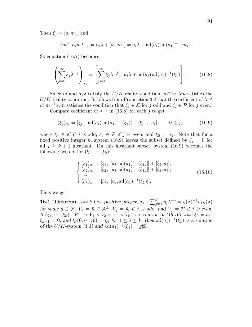
94
Then ξ1 = [a, m1] and
(m−1aimλ)+ = aiλ + [ai, m1] = aiλ + ad(ai) ad(a1)−1(m1).
So equation (16.7) becomes
∞∑
j=0
ξjλ−j
xi
=
∞∑
j=0
ξjλ−j , aiλ + ad(ai) ad(a1)−1(ξ1)
. (16.8)
Since m and a1λ satisfy the U/K-reality condition, m−1a1λm satisfies theU/K-reality condition. It follows from Proposition 3.2 that the coefficient of λ−j
of m−1a1m satisfies the condition that ξj ∈ K for j odd and ξj ∈ P for j even.Compare coefficient of λ−j in (16.8) for each j to get
(ξj)xi = [ξj , ad(ai) ad(a1)−1(ξ1)] + [ξj+1, ai], 0 ≤ j, (16.9)
where ξj ∈ K if j is odd, ξj ∈ P if j is even, and ξ0 = a1. Note that for afixed positive integer k, system (16.9) leaves the subset defined by ξj = 0 forall j ≥ k + 1 invariant. On this invariant subset, system (16.9) becomes thefollowing system for (ξ1, · · · , ξk):
(ξ1)xi = [ξ1, [ai, ad(a1)−1(ξ1)]] + [ξ2, ai],(ξ2)xi
= [ξ2, [ai, ad(a1)−1(ξ1)]] + [ξ3, ai],· · ·(ξk)xi
= [ξk, [ai, ad(a1)−1(ξ1)]].
(16.10)
Thus we get
16.1 Theorem. Let k be a positive integer, a1 +∑k
j=1 ηjλ−j = g(λ)−1a1g(λ)
for some g ∈ F , V1 = K ∩ A⊥, Vj = K if j is odd, and Vj = P if j is even.If (ξ1, · · · , ξk) : Rn → V1 × V2 × · · · × Vk is a solution of (16.10) with ξ0 = a1,ξk+1 = 0, and ξj(0, · · · , 0) = ηj for 1 ≤ j ≤ k, then ad(a1)−1(ξ1) is a solutionof the U/K-system (1.1) and ad(a1)−1(ξ1) = g"0.

95
Figure 1
Example 10.8 (i). A 2-tuple in R3 of type O(2) obtained by applyinga Ribaucour trasformation to a pair of lines

96
Figure 2
Example 10.8 (ii). A 2-tuple in R3 of type O(2) obtained by applyinga Ribaucour trasformation to a pair of lines

97
Figure 3
Example 10.10. K = −1 surfaces, top: case (1), bottom: case (2)

98
Figure 4
Example 13.2. An isothermic pair obtained by applyinga Darboux transformation to the isothermic pair of planes

99
Figure 5
Example 13.5. A CMC surface obtained by applying a Darboux transformation to a cylinderTop: surface Y1 for a = 2, cosh c = 2. Bottom: surface Y1 for a = 2, cosh c = 4.

100
Figure 6
Example 13.5. A CMC surface obtained by applying a Darboux transformation to a cylinderTop and bottom: two views of the surface Y1 for a = 2.75, cosh c = 9
4
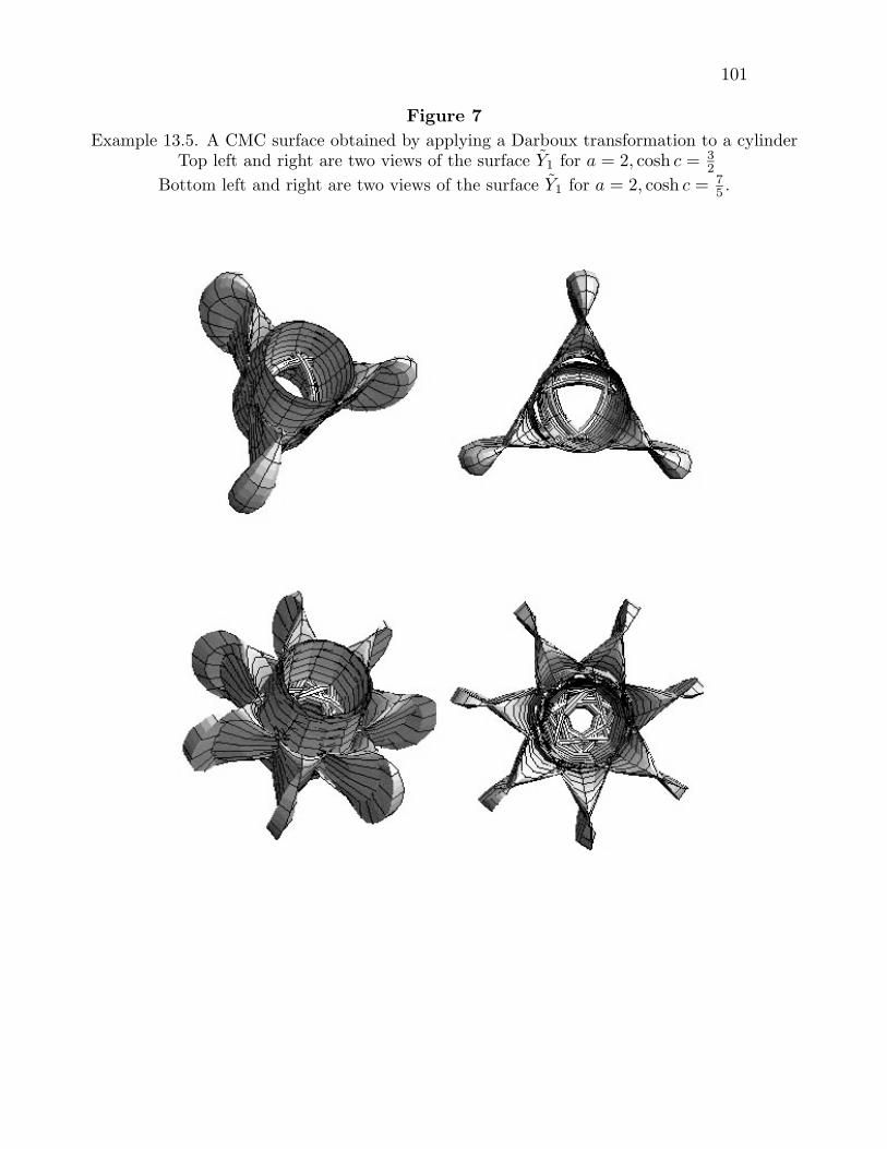
101
Figure 7Example 13.5. A CMC surface obtained by applying a Darboux transformation to a cylinder
Top left and right are two views of the surface Y1 for a = 2, cosh c = 32
Bottom left and right are two views of the surface Y1 for a = 2, cosh c = 75 .

102
References
[Ba] Backlund, A.V., Concerning surfaces with constant negative curvature. New Era Printing Co.,Lancaster, PA, 1905.
[BC] Beals, R., Coifman, R.R., Inverse scattering and evolution equations, Comm. Pure Appl. Math.38 (1985), 39-90.
[Bi1] Bianchi, L., Leconzioni di Geometria Differenziale. Bologna, 1927.[Bi2] Bianchi, L., Ricerce sulle superficie isoterme e sulla deformazione delle quadriche, Annali Math.
III 11 (1905), 93-157.[Bo1] Bobenko, A. I., All constant mean curvautre tori in R3, S3, H3 in terms of theta-functions,
Math. Ann. 290 (1991), 209-245.[Bo2] Bobenko, A. I., Surfaces in terms of 2 by 2 matrices, old and new integrable cases, Harmonic
maps and Integrable systems, edited by A.P. Fordy and J. Wood (1994), 83-127. Vieweg[Bo3] Bobenko, A.I., Exploring surfaces through methods for the theory of integrable systems, lectures
on the Bonnet porblem, preprint, math-dg/9909003[BFPP] Burstall, F., Ferus, D., Pedit, F., Pinkall, U., Harmonic tori in symmetric spaces and commuting
Hamiltonian systems on loop algebras, Ann. of Math. 138 (1993), 173-212.[BHPP] Burstall, F., Hertrich-Jeromin, U., Pedit, F., Pinkall, U., Curved flats and isothermic surfaces,
Math. Z. 225 (1997), 199-209.[Bu] Burstall, F., Isothermic surfaces: conformal geometry, Clifford algebras and integrable systems,
preprint, math-dg/0003096[Ca] E. Cartan, Sur les varietes de courbure constante d’un espace euclidien ou non-euclidien, Bull.
Soc. Math. France 47 (1919), 132-208.[Ch] Cherednik, I.V., Basic methods of soliton theory, Adv. ser. Math. Phys. v. 25. World Scientific,
1996.[CGS] Cieslinski, J., Goldstein, P., Sym, A., Isothermic surfaces in E3 as soliton surfaces, Phys. Lett.
A 205 (1995), 37-43.[Ci] Cieslinski, J., The Darboux-Bianchi transformation for isothermic surfaces, Differential Geom.
Appl. 7 (1997), 1-28.[C] Chen, B., Surfaces with a parallel isoperimetric section, Bull. Amer. Math. Soc. 79 (1973),
599-600.[DT] Dajczer, M., Tojeiro, R., Commuting Codazzi tensors and the Ribaucour transformation for
submanifolds, preprint[Da] G. Darboux, Lecon sur la theorie generale des surfaces. Chelsea, 1972. 3rd edition[FT] Faddeev, L.D., Takhtajan, L.A., Hamiltonian methods in the theory of solitons. Springer-Verlag,
1987.[FP1] Ferus, D., Pedit, F., Curved flats in symmetric spaces, Manuscripta Math. 91 (1996), 445-454.[FP2] Ferus, D., Pedit, F., Isometric immersions of space forms and soliton theory, Math. Ann. 305
(1996), 329-342.[H] Helgason, S., Differential Geometry, Lie Groups, and Symmetric Spaces. Academic Press, 1978.[HP] Hertrich-Jeromin, U., Pedit, F., Remarks on the Darboux transform of isothermic surfaces, Doc.
Math. 2 (1997), 313-333.

103
[HMN] Hertrich-Jeromin, U., Musso, E., Nicolodi, L., Mobius geometry of surfaces of constant meancurvature 1 in hyperbolic space, preprint math/9810157
[M] J. D. Moore, Isometric immersions of space forms in space forms, Pacific Jour. Math. 40 (1972),157-166.
[PiS] Pinkall. U., Stering, I., On the classification of constant mean curvature tori, Ann. of Math. 130(1989), 407-451.
[PS] Pressley, A. and Segal, G. B., Loop Groups. Oxford Science Publ., Clarendon Press, Oxford,1986.
[PT] Palais, R.S., Terng, C.L., Critical Point Theory and Submanifold Geometry. Lecture Notes inMath., Springer-verlag.
[Sa] Sattinger, D.H., Hamiltonian hierarchies on semi-simple Lie algebras, Stud. Appl. Math. 72(1984), 65-86.
[SZ1] Sattinger, D.H.,Zurkowski, V.D., Gauge theory of Backlund transformations. I, Dynamics ofinfinite dimensional systems, Nato Sci. Inst. Ser. F. Comput. Systems Sci. 37 (1987), 273-300.Springer-Verlag
[SZ2] Sattinger, D.H.,Zurkowski, V.D., Gauge theory of Backlund transformations. II, Physica 26D(1987), 225-250.
[Sy] Sym, A, Soliton surfaces, lett. Nuovo Cim. 33 (1982), 394-400.[Ten] Tenenblat, K., Backlund’s theorem for submanifolds of space forms and a generalized wave equa-
tion, Boll. Soc. Brasil. Mat. 16 (1985), 67-92.[TT] Tenenblat, K., Terng, C.L., Backlund’s theorem for n-dimensional submanifolds of R2n−1, Ann.
Math. 111 (1980), 477-490.[Te1] Terng, C.L., A higher dimensional generalization of the sine-Gordon equation and its soliton
theory, Ann. Math. 111 (1980), 491-510.[Te2] Terng, C.L., Soliton equations and differential geometry, J. Differential Geometry 45 (1997),
407-445.[TU1] Terng, C.L., Uhlenbeck, K., Poisson actions and scattering theory for integrable systems, Surveys
in Differential Geometry: Integrable systems (A supplement to J. Differential Geometry) 4 (1998),315-402. preprint dg-ga 9707004
[TU2] Terng, C.L., Uhlenbeck, K., Backlund transformations and loop group actions, Comm. Pure.Appl. Math. 53 (2000), 1-75.
[TU3] Terng, C.L., Uhlenbeck, K., Geometry of solitons, Notice, A.M.S. 47 (2000), 17-25.[U1] Uhlenbeck, K., Harmonic maps into Lie group (classical solutions of the Chiral model), J. Dif-
ferential Geometry 30 (1989), 1-50.[U2] Uhlenbeck, K., On the connection between harmonic maps and the self-dual Yang-Mills and the
sine-Gordon equations, Geometry & Physics 2 (1993), .[ZS] Zakharov, V.E., Shabat, A.B., Integration of non-linear equations of mathematical physics by
the inverse scattering method, II, Funct. Anal. Appl. 13 (1979), 166-174.[Zh] Zhou, Z.X., Darboux transformations for the twisted so(p, q)-system and local isometric im-
mersions of space forms, Inverse Problem 14 (1998), 1353-1370.

104
Authors’ addresses:(1) Martina Bruck, Institut fur Mathematik, Universitat Augsburg, Universitatstr. 8, D-86135 Augsburg, Germany, email:[email protected](2) Xi Du, Department of Mathematics, Northeastern Univ., Boston, MA 02115(3) Joonsang Park, Department of Mathematics, Dongguk Univ., Seoul, 100-715Korea, email:[email protected](4) Chuu-Lian Terng, Department of Mathematics, Northeastern Univ., Boston,MA 02115, email: [email protected]