Supply and Demand in a Public School Choice Program Randall Reback*

Barnard College and Teachers College, Columbia University Abstract: This study examines parents’ demand for sending their children to a public school located outside their residential school district. Using a unique data set that contains information concerning both inter-district transfers and rejections of transfer applications, I am able to identify which school district characteristics attract the greatest demand for incoming transfers. The analyses reveal that mean student test scores are stronger predictors of transfer demand than both students’ socio-economic characteristics and school district spending, suggesting that parents care more about outcomes than inputs. In addition, while districts are only supposed to reject transfer students due to capacity concerns, I find evidence that districts also constrain the supply of transfer spaces due to concerns about potential negative peer effects. These findings contribute to the literature concerning the parental demand for schooling and provide information concerning the possible effects of the No Child Left Behind Act’s school choice provisions on the redistribution of student enrollments. JEL: I20, I28, H73 Keywords: school choice, inter-district open enrollment, public school demand, Minnesota * rr2165@columbia.edu. Department of Economics, Barnard College, 3009 Broadway; New York, NY, 10027. Phone: 212-854-5005. Fax: 212-854-8947

1. Introduction

Many parents consider the local public schools when choosing their residence, and this behavior

is often referred to as traditional or Tiebout (1956) choice. Parents may also consider the availability and

affordability of private schools. The debate over school choice should thus not be framed as whether

parents and their children should have any school choice, but rather to what extent schooling options

should be formally expanded. While school choice debates often focus on voucher programs and charter

schools, intra- and inter-district transferring remain the most frequently used type of choice programs.

Many cities have formal intra-district open enrollment programs or magnet school programs that allow

students to attend a public school that is not in their local catchment area. The No Child Left Behind Act

has expanded intra-district public school choice throughout the country, because districts are supposed to

allow students to transfer out of any school designated as not meeting state standards for student

achievement. In addition, thirty-two states have formal inter-district open enrollment programs that allow

students to transfer to a public school outside of their residential district (Education Commission of the

States, 2003). This paper examines determinants of the demand and supply of transfer spaces in this type

of inter-district public school choice program.

The previous literature explicitly examining participation in public school choice has not been

able to separate supply side and demand side factors.1 Since transfer rates reflect the minimum of (1) the

supply of transfer spaces and (2) the number of students who would like to transfer, there is a serious

identification problem if one regresses transfer rates on explanatory variables. Many of these variables

may affect both the supply and demand for transfer spaces. For example, parents might prefer to send

their children to schools where students earn high test scores, but those types of schools might be 1 While some studies have used survey approaches to try to separately explain the demand for transferring (Armor & Peiser, 1997) or the supply of transfer spaces (Fowler, 1996), the accuracy of the survey responses is questionable. Examining inter-district choice in Massachusetts, Armor & Peiser (1997) find that families with participating children most commonly cited curriculum and academic standards as their reasons for transferring. However, Schneider & Buckley (2002) find that parents’ actual concerns, as measured by internet search patterns, often differ from their reported concerns. They found that parents in the Washington D.C. area, especially parent’s with college degrees, tend to be more interested in the demographics of the student body at the school than in school facilities, staff, programs, or even student test performance. While Fowler (1996) finds that the majority of districts in Ohio that did not allow incoming transfer students cited capacity concerns, the analysis in Section 6.3 of this paper reveals that districts often cite capacity concerns even when other factors appear more important in their decision.

1

relatively likely to restrict the supply of incoming transfer students due to concerns over potential

negative peer effects caused by incoming students with relatively low test scores.2 The reduced-form

relationship between transfer rates and mean test scores will thus reflect some combination of a positive

effect of test scores on demand and a negative effect of test scores on supply.

Using district-level data describing both student transfers and transfer application rejections, this

paper separately estimates the demand and supply of transfer spaces in an inter-district choice program. I

examine the demand and supply for transfer spaces in the nation’s oldest statewide inter-district choice

program, Minnesota’s open enrollment program. I measure transfer demand for each district by finding

the sum of incoming transfer students and rejected transfer applications. This may understate actual

demand in some cases, because any type of application process is potentially subject to endogeneity

whereby individuals are less likely to apply if they anticipate rejection. However, as discussed further

below, it appears that few interested individuals were dissuaded from applying to participate in this

particular program.

The results concerning the demand to participate in a choice program are somewhat similar to the

findings of the house price capitalization literature. In this literature, there is evidence that higher test

scores in local public schools lead to higher house values (Black ,1999; Downes & Zabel, 2002; Bayer,

Ferreira, & McMillan, 2004) through greater local housing demand from families with school-aged

children (Barrow, 2002).3 The results below suggest that similar factors influence families’ demand to

reside in one district but transfer their child to a non-residential school district. Transfer demand is

greatest when the mean student score on standardized tests in a district is much greater than in a

neighboring district.4 Relative values of student test scores are slightly stronger predictors of demand

2 Analyzing inter-district open enrollment in Massachusetts, Fossey (1994) finds that, compared to the districts receiving their students, districts that lost at least twenty residential students tended to have lower median family incomes and lower test scores in math and science than the receiving districts. Based on previous evidence, it is unclear whether these effects would be even larger if not for the supply-side decisions of school districts. 3 Figlio and Lucas (2004) also find that house values rise as a result of schools receiving higher ratings from accountability systems. 4 Through this paper, district X is considered a “neighboring district” to district Y if they are contiguous, sharing a geographic border at any location.

2

than relative values of socio-economic variables. Test scores have statistically significant effects on

demand even if one controls for socio-economic measures and school spending per pupil. While reliable

estimates of school productivity would incorporate value-added measures of student progress, this finding

is consistent with parents caring about a much rougher measure of productive schools: whether a school

produces higher than expected mean student test scores.

Yet the effects of test scores on transfer demand do not tell the entire story; students’ academic

performance also influences supply-side decision making. While Minnesota’s districts are not permitted

to selectively admit transfer applicants, they are allowed to reject one or more applicants due to capacity

concerns. Analyses of rejection patterns suggest that some districts cap the inflow of transfer students

due to reasons other than strains on capacity. Large differences in student test scores between the district

and one of its neighbors appear to be the most likely explanation for this behavior. Controlling for the

level of transfer demand, a district with substantially greater mean student test scores than a neighboring

district is significantly more likely to reject transfer applicants.

The next section describes Minnesota’s open enrollment program in more detail, Section 3

discusses possible influences on the demand and supply of transfer spaces, Section 4 describes this

paper’s data, Section 5 discusses the potential endogeneity of transfer applications, and Section 6

describes the empirical methods and results. Finally, Section 7 discusses the implications of these

findings for the design of school choice programs. Unless choice programs require that transfer

applications are only rejected based on specific capacity formulas rather than based on the discretion of

local school administrators, participation in inter-district open enrollment and intra-district programs such

as those from No Child Left Behind may be low in magnitude and rarely characterized by students

transferring to more productive schools.

2. Minnesota’s Open Enrollment Program

Minnesota’s inter-district open enrollment program allows children to attend public schools

located outside their residential district. The program became statewide in 1991, and participation rates

3

rose steadily throughout the early 90’s. In 1991, the average district lost about 2% of its residential

students to open enrollment, by 1997 this average climbed to 7%, and in 2000 the average was 6%.

Under the program, all students are entitled to attend their residential school district, but they may also

apply directly to other school districts if they would like to transfer. Students are free to simultaneously

apply to several non-residential school districts, and there are not any application fees. Once a student

transfers into a district, the student is entitled to remain in that district through high school graduation.

Districts may not selectively accept transfer applications. However, the law allows districts to

reject applications due to strains on capacity. If there is more than one school at the appropriate grade

level, transfer applicants may rank their choices of specific schools on their transfer application and it is

then up to district administrators to decide the highest ranked school in the district that has sufficient

capacity to serve the student. The district administrators may reject the application entirely if they feel

that there is not sufficient capacity in any of the listed buildings or in the district overall. If the district

feels that it has room for some but not all of the transfer applicants during a particular year, then it is

supposed to randomly choose applicants to fill the available spaces. State oversight of these rejections is

fairly loose. Districts do not have to provide any evidence of capacity constraints, and the state only

recently began collecting annual information from the districts concerning open enrollment rejections.

When a student transfers to a non-residential district, the residential district experiences a

financial loss equal to the non-compensatory aid per pupil that it receives from the state. The receiving

district gains an amount equal to the non-compensatory state aid per pupil that it receives from the state.

In 1999-2000, the year of this paper’s analyses, non-compensatory aid per student equaled about $4,000,

varying across districts by only a couple of hundred dollars. While the financial award was far less than

the average district’s per pupil spending in Minnesota (about $7,000), this financial award usually

exceeds the marginal cost of serving these additional students due to economies of scale.5

5 Even when special education students transfer, the residential district must compensate the receiving district for special needs such as transportation, so that the net marginal cost of receiving a special education student may not be much larger than for another student.

4

In addition to the inter-district open enrollment program, Minnesota offers a variety of other types

of school choice programs. Minnesota offers charter schools which are legally independent from public

school districts, receive state funding but no local funding, and may be started by one or more licensed

teachers.6 The majority of the charter schools existing during 2000 were located in the two school

districts that serve the twin cities of Minneapolis and St. Paul. These two districts also offer a wide array

of intra-district school choice, such as magnet schools that are attended by students from various

neighborhoods within each city. Since these extensive charter school and magnet school programs are

mostly limited to two school districts, the presence of these programs likely has only a minor effect on

this paper’s district-level analyses. In order to further ensure that the availability of outside choice

options does not bias the results, additional analyses of this paper’s models add control variables based on

the local presence of charter schools and private schools.

3. Theoretical Sources of the Demand and Supply of Transfer Spaces

3.1 Demand

Demand for inter-district choice occurs when a family chooses to reside in one school district but

wants their child to attend public schools in a different district. This section presents a simple model of a

household’s location decision and the ensuing decision of whether to apply to transfer to other districts.

While the theoretical framework focuses on district-level characteristics, ignoring heterogeneity across

schools within the same district, some of the empirical analyses below verify that within-district school

heterogeneity does not significantly influence the supply or demand for transfer spaces in Minnesota.

Define Qj as a vector of attributes of the educational services offered by school district j. Let Hj

equal a vector of all other attributes of the housing, services, and location offered by district j. For

simplicity, assume that all of the housing within district j is homogenous and assume that households only

have one child. Define cjk as the transportation costs, in terms of both time and private expenditures,

6 Charter school policy information provided by the Education Commission of the States at http://mb2.ecs.org/reports/Report.aspx?id=65.

5

associated with living in district j and sending a child to school in district k. Consider household i’s

indirect utility function, virk(Qk,Hr,crk), where the household resides in district r and receives educational

services from district k. Households may have heterogeneous preferences, particularly with regards to the

types of school district characteristics that they value.

If a household resides in district r, then they are guaranteed the option of setting Qk=Qr. The

household must first choose where to live, in light of these characteristics and the equilibrium house

prices and tax rates. Suppose that there are three districts: district A, district B, and district C. Without

loss of generality, assign district B and district C so that viAB>viAC. Define pk ]1,0[∈ as the expected

probability of being allowed to send a child to district k while living in another district. We can then

define a household’s expected indirect utility from living in district A, bar, iAv , as follows:

iAv = viAA if viAA>viAB>viAC

(1) = pBviAB + (1 – pB)viAA if viAB>viAA>viAC

= pBviAB + pC(1 – pB)viAB + (1-pC)(1-pB)viAA if viAB>viAC>viAA

Assuming that a household is risk neutral, it will choose to reside in district r if:

(2) srvv isir ≠∀>

The equilibrium supply and demand in this model is complicated, because this household location

decision is influenced by the endogenously determine transfer application acceptance probabilities. The

analyses in this paper will measure the transfer demand for each district after residential location

decisions and these endogenous transfer acceptance probabilities have reached a long-run equilibrium.

After the residential location decision, the household must decide whether to apply to transfer to other

districts. The household residing in district r will apply to transfer to district j if virj>virr. This assumes

that there are not any application costs, which is true for the program examined in this paper.

Note that there are two general cases in which virj>virr. First, this could be an attempt of household i

to free-ride on district k’s premium services. In this case, the majority of households prefer district k

6

where housing thus becomes more expensive than in district j. Second, it could be true that virj>vijj due to

the idiosyncratic preferences of household i, which may have unique reasons for placing a high value on

either housing in district j or schooling in district k (or both). Both idiosyncratic preferences and attempts

at free-riding could thus explain why people apply to transfer under an open enrollment program.

With Nj households in the remainder of the state outside district j, the demand to transfer into

district j in terms of the number of interested transfer students will equal:

(3) Dj=∑ , =

>jN

i 1irrirj1 )v(vI

where equals one if and equals zero otherwise. )v(vI irrirj1 > ijrijk vv >

Note that transfer demand is defined as the number of applicants, so that a household might demand to

transfer into district j from district r but also demand to transfer into district k from district r. By using

this type of transfer demand, this paper implicitly focuses on estimating which factors make district j

preferred to district r, regardless of the relative merits of transferring to either district j or district k.

Equation (3) suggests that there should be high demand to transfer into district j when the

characteristics of district j, Qj, are relatively desirable compared to nearby districts, while the

transportation cost of transferring to district j from a less desirable district is low.

3.2 Supply

An administrator in each district must decide how many inter-district transfer students it is willing

to accept. Let equal the number of transfer students enrolled in district j. There will be several

potentially important factors determining the level of that district j’s administrator prefer.

jT

jT

Define mj( ) as the marginal cost from allowing incoming transfer students while

maintaining the same quality of educational services for residential students as if there were not any

transfer students entering. This marginal cost will include both the direct costs associated with providing

services for transfer students, as well as the net cost of any peer effects caused by these transfer students.

jT jT

7

(Incoming transfer students could create negative peer effects which increase the marginal cost, or these

transfer students could create positive peer effects which decrease the marginal cost or even lead to

negative net costs.) This marginal cost will also include the costs of compensating for any loss of school

district revenue due to capitalization effects. When students are able to transfer into a popular school

district, the erosion of the housing premium can decrease the housing prices in that district, which in turn

leads to a smaller local property tax base (Reback, 2005).

Define hj( ) as an index of the value of any positive reputation effects from admitting transfer

students. If there is asymmetric information, transferring may increase the overall popularity of the

school district by sending a message to other parents that some parents think that this is a superior school

district.

jT

Let gj( ) equal the level of residents’ discontent over incoming transfer students. Holding

actual school quality constant, there are several reasons why incoming transfer students could decrease

residents’ welfare. First, this incoming transferring could decrease local house prices. Second, the

residents may perceive that the incoming transfer students lead to more negative peer effects than the

actual peer effects.

jT

Finally, define q( ) as an index of the state’s satisfaction that district j is in compliance with the

state’s open enrollment law. Even if the other factors imply that the district should not accept many

transfer students, the district administrator may be concerned with whether it appears to be following the

law’s guidelines.

jT

The function measuring the combined impact of these supply-side factors will vary across

districts, as some districts’ administrators will prioritize certain objectives more than others. Define as

the maximum level of that district j’s administrator decides to allow. District j’s administrator will

choose to maximize some function of these factors:

jS

jT

jS

(4) fj( *Subsidy - m( ), g( ), h( ), q( )). jS jS jS jS jS

8

The first term represents the net financial gain to the district, which equals the number of

incoming transfers multiplied by the per student subsidy for serving these students minus the marginal

cost of serving these students. As mentioned earlier, this subsidy equaled about $4000 per student in

Minnesota during this paper’s sample period, varying by only a couple of hundred dollars across districts.

3.3 Equilibrium

Unlike most other markets, there is no price mechanism to guarantee that the market for inter-

district transfers clears. The actual number of accepted transfer applicants will equal the minimum of the

supply and demand for transferring. The number of accepted transfer applicants, , will be: *jT

(5) = min[Sj,Dj] *jT

This simple theoretical analysis highlights some important considerations for empirically

analyzing the inter-district transferring market. First, transfer demand may come from both households

seeking to enhance school quality without paying a housing premium and from households with

idiosyncratic preferences. Second, most variables that may have positive effects on demand may also be

associated with lower levels of supply. For example, based on the house price capitalization literature, a

district with greater student test scores than a neighboring district would be likely to receive a high level

of demand, because these test scores seem to be positively correlated with valued characteristics of school

quality (Qj). On the other hand, concerns over negative peer effects or negative capitalization effects may

cause these same districts to provide a relatively low supply of transfer spaces. The theoretical

equilibrium relationship between transferring and factors such as student test scores is thus ambiguous,

and explaining the observed equilibrium requires a separate analysis of demand and supply.

4. Data

This paper’s data allows one to estimate which observable variables are important components of

inter-district demand, i.e., which variables should be included in the Qk vector in households’ indirect

9

utility functions. Fortunately, these data include both transfer rates and rejection rates, so that one may

estimate the transfer demand to enter each school district (Dj) without worrying about the confounding

effects of the supply of spaces in that district (Sj). Less fortunately, these data are also highly aggregated,

which slightly limits how precisely one may estimate the parameters described above. In particular, the

data are at the district-level rather than the household level, and the data do not reveal the number of

students that transfer out of a particular district and into another particular district but simply reveal the

total number of exiting and incoming students in each district. By incorporating geographic information,

the empirical strategy described below is to exploit information about districts’ neighbors in order to

characterize the likely transfer decisions that are most relevant to students.

The data combine several, school-district level data sets provided by the Minnesota Department

of Education. In order to capture the long-run transfer equilibrium, after general equilibrium effects

related to families’ location decisions have occurred, I focus on inter-district choice during the 1999-2000

school year, nine years after the beginning of statewide open enrollment. Explanatory variables come

from Minnesota’s School District Profiles (2000), as well as district-level data from the Minnesota

Department of Education’s website describing mean student test scores on standardized, statewide exams

for students in third, fifth, and eighth grade.7 The two data sets of particular importance are the open

enrollment transfer rate data and the open enrollment application rejections rate data. District-level open

enrollment transfer flow data are available for the 1999-2000 school year, provided directly from the

Minnesota Department of Education. These flows reveal the number of students residing in each school

district that attend a different school district (i.e., outgoing transfer students), as well as the number of

students attending the school district that do not reside in the school district (i.e., incoming transfer

students).

Incoming transfer flows, but not outgoing flows, are also available broken down by race and by

two other categories: whether the student has been designated for special education services and whether

7 The district-level test score measures used in this paper equal the average of the mean student test scores in third, fifth, and eight grade in reading and math during the 1998-99 school year.

10

the student is eligible for free or reduced priced lunches due to membership in a low-income family. The

transfer flows do not include breakdowns by grade.

District-level open enrollment rejection data are available for the 1998-99, 1999-2000, and 2000-

2001 school years. These data are the results of district responses to an annual survey given by the

Minnesota Department of Education in which districts list the number of rejected open enrollment transfer

applications by grade and by the reason for the rejection. The response rate to this survey was 338 out of

345 in 1999-2000, and was fairly similar for 1998-99 and 200-2001.8 The vast majority of school

districts do not reject any transfer applications in a particular year. Only 8%, 8%, and 10% of responding

districts reject any new applications in 1998-99, 1999-2000, and 2000-2001 respectively, and some of

these might have accepted some new applicants at the same time that they rejected others. Only five

districts did not receive any transfer students during 1999-2000. The data do not provide any information

about characteristics of the students applying to transfer. The presence of rejections data from the years

immediately surrounding 1999-2000 is useful for conducting the analysis below given the potentially

endogenous nature of any type of application.

The open enrollment transfer and rejection data are combined with district-level data concerning

characteristics of residents, school expenditures, student test scores, total enrollments by grade, and total

enrollments by race. The analyses also utilize geographic data concerning which districts are contiguous,

(sharing a border at some geographic location). One can thus analyze the supply and demand for

schooling based on both a district’s own characteristics and the characteristics of neighboring districts.

This is particularly helpful, since anecdotal evidence suggests that most transferring students attend a

school in a neighboring district. Table 1 displays descriptive statistics for variables used in the regression

analyses. Out of the 345 districts in operation during the 1999-2000 school year, 2 newly formed districts

are omitted from the regression analyses of transfer demand due to missing values for several variables, 7

8 The exact response rate and information concerning which districts did not respond is only available for 1999-2000.

11

other districts are omitted due to missing financial data or test score data, and 7 others are omitted

because they did not respond to the transfer applicant rejections survey.

The regression results remain nearly identical when one includes this latter group of non-

responding districts and assumes that they did not reject any applicants. This assumption seems close to

reality, because none of these districts reported rejecting any students during the previous or latter year.

In addition, these districts possess similar observed characteristics as districts that did not reject any

applicants. These non-responding districts may have mistakenly believed that they need not return the

survey form unless they had rejected any applicants.

5. How Endogenous were Applications?

Applications may be endogenous because people’s perceived probability of acceptance influences

their application decision. If potential applicants are deterred from applying because they anticipate

rejection, then the sum of transfer students and rejected applicants may understate true demand.

However, in the case of inter-district transferring in Minnesota, few people likely withheld applications

because they anticipated rejection. As described in Section 6.3 below, rejections were uncommon.

Furthermore, there were not any application fees, and applying to one district did not preclude applying to

others. The only costs associated with applying would be the cost of gathering information about schools,

the cost of time to obtain and submit an application, possibly the cost of a stamp to mail the application,

and the potential emotional disappointment associated with a rejection. Because rejections were not made

based on personal student characteristics, the emotional disappointment of a rejection may not have been

high for most parents compared to the perceived benefits from a successful transfer application. Given

these low costs and the high probability of success, most parents likely would apply to transfer their child

even if they were uncertain about whether their child should transfer or if they did not feel very strongly

about the transfer opportunity.

Examining a subset of districts, those neighboring Minneapolis, there is some empirical evidence

which supports the idea that interested applicants did apply during the sample period. One year after this

12

paper’s sample period, there was an out-of-court settlement of an adequacy lawsuit brought by the

Minneapolis branch of the NAACP against the state of Minnesota. As a result of this settlement, students

from low income families residing in the Minneapolis urban school district were guaranteed access to a

minimum number of transfer spaces in nearby, suburban districts. In particular, students were eligible to

transfer to the suburban districts if their family’s income was sufficiently low that the student qualified for

federally subsidized lunches. Participants in this new program may or may not have transferred across

districts through regular open enrollment if this new program did not exist. Some participants in this new

program may have been induced to participate due to the new advertising or larger overall participation

rates created by the program. Other participants in this new program would have applied and been

rejected through regular open enrollment applications. Finally, some participants in this new program

would not have bothered to apply through regular open enrollment because they would have anticipated

rejection.

This latter category is the potential cause for concern in this paper’s analyses of open enrollment

demand, and it does not appear that many students fit into this category. Table 2 compares the number of

subsidized lunch transfer students during 1999-2000 (this paper’s main sample period) to the number of

subsidized lunch transfer students into the participating suburban districts in 2001-02 and 2002-03 when

the new program was first in effect.9 While the suburban districts had recruitment targets that may have

induced students to temporarily participate, Table 2 reveals that the number of these students who used

the program for consecutive years was generally similar to the number of these types of students using

open enrollment before this program began. Only two out of the eight suburban districts experienced a

non-trivial increase in incoming transfer students from low income families, and one of these two districts

9 The number of Title I transfer students in 1999-2000 may slightly overstate the number of Title I transfer students who resided in the Minneapolis district, because incoming Title I transfer students in the suburbs may have come from other suburban districts. However, this type of transfer was probably uncommon due to the higher incomes generally found in the suburban districts.

13

had a high enough rejection rate in 1999-2000 to explain this increase.10 While this analysis only covers a

few suburban districts, it is noteworthy that summing the number of incoming transfers and the number of

rejected applicants does not appear to cause one to systematically underestimate district-level demand.

Data concerning rejections from the years immediately before and after this paper’s main sample

period (1999-2000) provide further evidence that the estimates are not strongly influenced by the potential

endogeneity of applications. People might not continue to apply each year if they had been previously

rejected, so that it is important to check whether the results would be influenced by year to year deferment

of applications. Twelve out of twenty-seven districts that rejected applicants in 1998-1999 also rejected

applicants in 1999-2000, while sixteen out of twenty-six districts that rejected applicants in 1999-2000

also rejected applicants in 2000-2001. Fortunately, all of the qualitative results below concerning transfer

demand in 1999-2000 remain similar when one controls for rejections made during the previous year and

rejections made during the following year. This confirms that the results are not biased from a transitory

component of endogenous applications.

6. Empirical Analyses

The first subsection below describes rates of participation in open enrollment and describes the

districts that experienced relatively large inflows or outflows of transfer students. The next subsection

analyzes the demand for transferring into districts, and the third subsection analyzes cases in which

supply is binding so that the district rejects some transfer applicants. The final subsection describes the

effect of transferring on the distribution of students across districts, including the impact on racial

segregation across school districts.

6.1 Descriptive Statistics

Transfer rates for various types of student populations are displayed in Table 3, along with the

populations’ overall representation in Minnesota public schools. Non-white students are less likely to

10 The total number of rejections for one of these two districts was approximately as large as the increase in incoming transfers reported in Table 2. (As a condition of receiving the raw, district-level rejections data, I agreed not to report the number of rejections by district.)

14

participate, students from low income families (eligible for federally subsidized school lunches) are

slightly more likely to participate, and special education students are slightly more likely to participate.

Examining entrants into lotteries for intra-district transferring in Chicago, Cullen, Jacob, & Levitt (2003)

also observe lower participation rates among non-white students, but found lower participation among

students from low-income families as well.

Table 4 shows characteristics of districts that were strongly affected by open enrollment

transferring. All types of high impact districts, both those gaining and losing students, tend to have

smaller median household income than the median district in the state (displayed in Table 1). This may

be due to wealthier families having an easier time satisfying their schooling preferences through

traditional Tiebout choice and private schooling options. The forty-four districts with net gains in transfer

students equal to at least ten percent of their residential enrollments tend to have higher test scores and per

pupil spending than the median district in the state, but are fairly similar along other dimensions.

Regression analyses are necessary to parse out which of these variables are actually influencing transfer

demand. Many of these variables are highly correlated and transfer demand may be strongly influenced

by districts’ characteristics relative to neighboring characteristics.

6.2 Demand for Public School Transfer Spaces

I estimate the demand to transfer into district j, Dj, by finding the sum of incoming transfer

students and the number of rejected applicants. The following model is used to predict transfer demand:

(6) log(Dj) = α + β1log(# of Householdsj) + β2log(Population Densityj) + β3(% of Students

in Elementary Gradesj) + β4(% of Students in Middle School Gradesj) + Xj β5

+ neighborsjX , β6 + β7 + εj. min,neighborsjX

The dependent variable equals the natural logarithm of the sum of incoming transfer students and

the number of rejected applicants in district j during 1999-2000. One may thus interpret the coefficients

in terms of percent changes in the number of students who would like to transfer into the district. The

15

qualitative results remain nearly identical if one replaces this dependent variable with one that divides the

level of demand by some measure of school district size, such as total residential enrollment.

The first four independent variables are control variables accounting for structural differences

across districts which may be related to the number of students seeking to transfer into the district. These

control variables are the number of households in the district, the population density in the district, the

fraction of public school students enrolled in elementary grades (Kindergarten through grade 5), and the

fraction enrolled in middle school grades (grades 6 through 8).

The Xj vector contains various combinations of independent variables that might predict demand,

and the purpose of this analysis is to determine the relative importance of these variables. In order to

facilitate the comparisons of these variables and their predictive validity, they are all converted into

standard normal values across the sample (i.e., Z-scores). The demand for transferring into a district is

likely based on both characteristics of district j and characteristics of neighboring districts. There might

be greater demand to transfer into district j if a nearby district is significantly worse along some quality

measure or if many nearby districts are worse along this quality measure. Vector therefore

includes the Z-score of the minimum value of these characteristics among district j’s neighbors, and

Vector

min,neighborsjX

neighborsjX , contains the Z-score of the population size-weighted mean value of these characteristics

for district j’s neighbors.

In the full model, these vectors include all of the district-level variables listed in Table 1: median

income of residents, mean house value of residents, education levels of residents, per pupil expenditures,

local revenues per pupil, and mean student scores on standardized tests. One should note that the mean

test scores may be slightly influenced by the performance of incoming transfer students, because separate

test score data for residential and transfer students are not available.11 Because net transfer rates will also

11 Test scores predating the open enrollment program are also not available.

16

affect per pupil expenditures and revenues, I do not use the actual values of these variables, but instead

estimate their hypothetical values if no students transferred.12

Additional regression models, not shown here, add four control variables for alternative school

choice mechanisms: the log of private school enrollment in the district, the log of private school

enrollment among the district’s neighbors, the log of charter school enrollment in the district, and the log

of charter schools enrollment in the district neighbors. The results below remain nearly identical after the

inclusion of these control variables, and the coefficients of these four control variables are very small. Of

the four, only private school enrollment in the district is ever statistically significant, as it is mildly,

negatively related to transfer demand.

6.2.1 Demand Related to Free-Riding

Table 5a reveals the explanatory power of various types of variables when they are included

alone. The focus of Table 5a is on variables that might be related to the free-riding type of transfer

demand discussed in Section 3.1, whereby students are transferring to a district that is considered to be of

higher quality than their residential district. Aside from the inclusion of the structural control variables,

Table 5a reveals the “raw validity” of various factors, the predictive power when one factor is included on

the right-hand side of the model and other factors are omitted. The structural control variables alone

actually explain 43.4% of the variation in demand, so the bottom row of Table 5a reports how much of

the remaining variation is explained by a particular factor. The direction and statistical significance of the

coefficients are similar for test scores, household income, and home values: demand is greater when a

district has higher levels of these seemingly desirable characteristics and demand is greater when at least

one of the district’s neighbors has relatively low levels of these characteristics. Average characteristics of

a district’s neighbors are far less important predictors of transfer demand than the minimum value among

neighbors, both in terms of magnitude and statistical significance. Excluding the average neighbor

characteristics from these regressions has little impact on the other coefficients or on the relative

12 I estimate hypothetical total expenditures by subtracting the net amount of state aid gained by the district due to incoming and outgoing transfers, and then I divided this total expenditure measure by the number of public school students who reside in the district regardless of whether they actually remain in the local public schools.

17

predictive validity of the various types of variables. The amount of explained variation in the demand for

transfer spaces is fairly similar for each type of district characteristic, with R2’s equal to .456, .447, or

.464, respectively when mean household income, median house value, or mean student test score are used

as independent variables. Average math test scores predict demand better than average reading test

scores.

Figure 1 illustrates how the demand for transferring varies based on the mean household income

in districts. In order to adjust for differences in population density, Figure 1 defines district demand as

the number of incoming transfers divided by the number of residential students. One can see in Figure 1

that districts tend to experience high demand when median household incomes is in a higher range than in

one of the neighboring districts. Figure 1 also shows that districts tend to be clustered around other

districts with similar median household incomes, so that the demand for transferring could be even greater

for public school choice programs in geographic areas more spatially heterogeneous than Minnesota.

Column 8 of Table 5a reveals that the total spending per pupil variables, which adjust for

transferring patterns (see footnote 12), do not have statistically significant effects on transfer demand.

This is not very surprising, since expenditures per pupil will reflect a combination of local funding, state,

and federal funding. While local funding is likely associated with desirable characteristics such as

property wealth and parental interest in schooling, other funding may be linked to undesirable

characteristics such as high poverty rates and low property wealth. Overall, spending per pupil across

Minnesota school districts is negatively correlated with potentially valued characteristics such as median

income, so the popularity of districts with higher socio-economic characteristics may cancel out the

popularity of districts that spend greater amounts per pupil.

In order to isolate spending that should not be linked to any negative traits, column 9 of Table 5a

focuses on local revenue per residential pupil. Presumably parents would be thrilled to send their child to

a district where other parents make sizable financial contributions to school expenditures. In fact,

demand to transfer is greater for districts where the average local expenditures of neighboring districts is

relatively large and for districts where the minimum local expenditure level among the neighboring

18

districts is relatively low. The latter finding is intuitive, parents from the low spending district may want

to upgrade to a higher spending district. One possible explanation for the former finding is that parents

residing in districts with high local tax rates and large local property tax bases care a lot about their

children’s schooling and are not always satisfied with the local schools, so they are more likely to send

their children to a neighboring district even if this district has lower per pupil expenditures.

The final two columns of Table 5a reveal the effects of parental education levels on transfer

demand. Transfer demand is greater when a district has fewer high school dropouts or when a district’s

least educated neighbor has fewer residents with Bachelor’s degrees. These findings are consistent with

the idea that parents want to transfer their children into districts with better educated parents. The raw

validity of these variables are fairly low, so much of this finding may simply be due to a positive

correlation between parental education and another valued trait such as student test scores or parental

wealth.

In addition to raw validity, it is important to determine the incremental validity of various

predictors of the demand for choice. In particular, how does the amount of explained variance in demand

decrease when only one type of variable is omitted? The first column of Table 5b displays the regression

results when all of the independent variables are included, and the other columns display results when

certain variables are omitted. The coefficients generally retain their sign from Table 5a. The R-squared

when all variables are included equals .54, a moderate increase from the models of Table 5a that only

included one type of predictor. The R-squared does not decrease much when any one type of variable is

omitted, partly because these variables are positively correlated. There is a .43 correlation between mean

test score and median income, a .37 correlation between mean test score and mean house value, and a .88

correlation between median income and mean house value.

Columns 1 and 2 of Table 5b reveal that the inclusion of the mean test score variables allows one

to explain an additional 2% of the variance in demand, even when the model already controls for socio-

economic characteristics and per pupil spending. The F-test comparing these two regression models

confirms that, at the .01 level of significance, one can reject the null hypothesis that the test score

19

variables’ coefficients equal zero. This suggests that transfers flow towards schools with higher outputs,

even controlling for schools’ inputs. This provides some tentative evidence that public school choice

could lead students to move to more productive districts, in which students earn higher test scores than

one would predict from the included socio-economic and spending variables. There are several reasons

why one should interpret this result very cautiously. First, as previously stated, the test score variable

measures the performance of the actual students served, so that the average test score is slightly

influenced by whether student inflows and outflows improve the mean student ability level. Second, it is

possible that the schools with higher than predicted test scores are not truly more productive, but simply

have students with high academic abilities related to unobserved, non-school factors or students who

enjoy positive peer interactions. Third, the students who use the choice program may not necessarily

improve their own performance as a result (Cullen, Jacob, & Levitt, 2003, 2005). Fourth, while this

analysis focuses on student sorting, a school choice program could also directly affect schools’

productivity through competition or changes in funding.

Given that parents are able to express a preference for their child to transfer to particular schools

within a non-residential district, an important robustness check is to determine whether within district

school heterogeneity influences transfer demand. While school-level data are not available for all of the

descriptive characteristics, they are available for student test scores, the variables at the district-level

which bests predict transfer demand. When one adds either the standard deviation in school-level mean

test scores or the maximum school-level mean test score in a particular grade as an additional control

variable in the models from equation (6), this variable is statistically insignificant and the models continue

to explain roughly the same proportion of the variance in transfer demand.13 Either most transfer

applicants are enticed by overall district characteristics or these characteristics seem to proxy well for the

qualities of particular schools that these applicants find attractive.

13 For example, suppose that one re-estimates the model in column 4 in Table 4a with the mean math test scores specifically for 5th grade students in the district. If one adds an independent variable equal to the Z-score for the maximum school-level mean 5th grade student math test score found in the district, this additional variable has a coefficient of .067 with a standard error of .154. The R-squared only increases from .466 to .468 with the addition of this maximum school-level mean test score variable.

20

6.2.2 Demand Related to Tastes for Differentiated Products

Another important robustness check for these analyses is to determine whether the previous

estimates might be biased in either direction by transfer demand related to horizontal competition between

districts. While it is generally difficult to measure idiosyncratic preferences, there are certain measurable

characteristics of districts that might differentiate them from one another and thus influence transfer

demand. I add a few of these measures that are likely to be exogenous, i.e., not influenced by the actual

transfer students who enter the schools. These variables include the fraction of spending that is dedicated

to vocational education, the fraction of spending that is used for community service purposes, and the

average and minimum neighboring districts’ values for these vocational and community service variables.

As with the earlier variables, each of these variables is included in the form of a Z-score. In addition, I

explore whether transfer demand is related to indicators for whether the district has a highly successful

hockey team or football team, a team that has gone to the state finals in its division during either of the

two years prior to the sample period. These sports are very popular in Minnesota and there is anecdotal

evidence of students being recruited for athletic purposes.

The inclusion of these additional variables does little to change the results from Table 5b. For

example, the estimated coefficient on the test variable in this expanded model equals .225 with a .069

standard error, as opposed to .216 with a .067 standard error in the first column of Table 5b. The

estimated coefficients of these additional variables when they are added to the full model (column 1 of

Table 5b) are displayed in Table 6. There is slightly greater transfer demand when districts spend a

greater proportion of their budgets on vocational programs than neighboring districts. This is probably

due to a few students who prefer a school district offering these specialized services. When neighboring

districts spend a relatively large fraction of their budgets on community service programs, there is less

demand to transfer into a district. This may be due to increased loyalty to the local, residential schools in

districts that have greater interactions with their communities. Successful hockey or football teams do not

increase transfer demand; in fact, districts with successful football teams receive less transfer demand

than other districts. It is possible that few students are recruited to transfer in order to play for the best

21

teams, and it is also possible that an even greater number of students are dissuaded from transferring into

a district where it may be more difficult for them to play on the teams. The results remain similar if one

replaces these indicator variables with the number of successful teams per residential student served.

6.3 The Supply of Transfer Spaces

Unlike demand, one cannot precisely estimate the supply of transfer spaces; one only observes

supply in the few cases that it is binding because a district rejects an applicant. The data allow one to

characterize reported reasons for these rejections and to compare districts receiving similar levels of

demand but making different decisions concerning rejecting applicants. Only 26 districts (about 8% of

respondents) rejected any applications for 1999-2000. Responding to a closed-ended survey, districts

gave reasons for these rejections which included lack of capacity in a program (31% of rejections), lack of

capacity in a class (23% of rejections), lack of capacity in a school building (28% of rejections), and other

reasons (18% of rejections). Districts with court-ordered desegregation plans were also permitted to cite

racial balance concerns as a reason for rejections, but none did so. Districts using certain explanations for

rejections possess fairly similar characteristics as districts using other explanations, though the small

number of rejecting districts weakens one’s ability to formally test for differences within the group of

rejecting districts.

It is possible that the low rates of rejections in Minnesota are related to school districts’ ability to

expand capital resources, such as the number of classrooms, over time. Examining Milwaukee’s private

school voucher program, Belfield, Levin, & Schwartz (2003) find that nearly half of the participating

private schools in 2002 were founded after the program began. The long-run supply of transfer spaces

under inter-district enrollment may also be somewhat elastic, especially given that about 5% of

Minnesota’s districts experienced net gains of transfer students equal to at least 20% of the size of their

residential student population.

Given that few districts rejected applicants, it is difficult to precisely estimate how various factors

simultaneously influenced the probability that a district’s supply of transfer spaces was binding. In light

of this limitation, this section uses a non-parametric approach to analyze these supply-side decisions.

22

Table 7 describes characteristics that influence whether a district is more likely to reject any transfer

applicants, sorted by the magnitude of demand for transfer spaces in the district. Table 7 focuses on two

characteristics that are important determinants of whether the supply of spaces is binding: (1) whether the

district was at maximum capacity in terms of enrollment history from the previous five years, and (2)

whether the district’s mean test scores are at least one standard deviation greater than one of its

neighboring districts. Districts that reject applicants are significantly more likely to be at a historically

high enrollment level or to have much higher test scores than a neighboring district. In fact, 69 percent of

the districts that rejected transfer applicants met at least one of these two conditions, while only 34

percent of the districts that did not reject any applicants met one of these two conditions. As shown in

column 4 of the bottom panel of Table 7, these differences usually remain statistically significant when

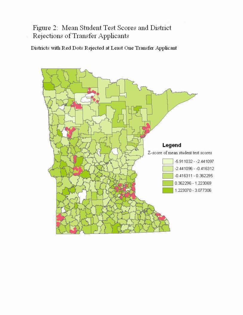
one compares districts with similar levels of transfer demand. Figure 2 illustrates the relationship

between mean student test scores in each district and whether the district rejected any transfer applicants.

One can observe that many of the districts that rejected transfer applicants had much greater test scores

than at least one nearby district.

Although some transfer applicants may have requested specific schools, within-district

heterogeneity does not appear to influence supply decisions. The difference between the highest school-

level mean test score in the district and the minimum district-level mean test score among neighboring

districts does not predict rejections as well as the district-level test score gaps shown in Table 7 predict

rejections. This finding even holds if the analysis only includes rejections that districts claimed were due

to “lack of capacity in a school building.”

Aside from mean student test scores, districts that rejected or did not reject applicants were not

significantly different from each other. Large gaps in average house values or in median household

income between a district and one of its neighbors were only slightly more common among districts that

rejected transfer students. The greater importance of test scores might reflect administrators’ concerns

over the potential peer effects from admitting transferring students.

23

6.4 Effects of Student Transferring on Segregation Across School Districts

Given that peer characteristics are correlated with both the supply and demand for transfer spaces,

it may be important to examine whether the actual equilibrium transfers influence the segregation of

students across school districts. Estimates of the effects of incoming transfer students on various forms of

segregation across districts are displayed in Table 8. Due to the lack of data concerning exit patterns,

these estimates only capture the impact of destination school district characteristics on segregation, as if

any student who exits under the open enrollment program would not have attended any Minnesota public

school in the absence of the program. Another important caveat is that this analysis does not consider the

effects of the school choice policy on residential sorting, which may in turn influence the distribution of

residential students across public school districts (Nechyba, 2003). The first column of Table 8 reveals

that, of the three student subgroup categories, only non-white students were substantially more likely to

choose a school district with higher representation of that group than the median district. The next two

columns of Table 8 show indexes of dissimilarity based on net-of-transfer enrollments (i.e., observed

enrollments in light of the policy) and based on residential enrollments (i.e., students who reside in the

district and remain in the district’s public schools). Dissimilarity indexes may be interpreted as the

minimum fraction of students that one could reassign in order for the fraction of students in the subgroup

in each district to equal the fraction of students in this subgroup in the entire Minnesota public school

system.14

The estimates in Table 8 reveal a trivial impact of incoming transfer students on statewide

segregation across districts by race, family income, or special education status. The changes in the

segregation indexes by race and by special education are each less than 2% of the size of the rate of

participation in open enrollment. In other words, one would have to re-assign less than 2% of all

transferring students in order to achieve similar segregation patterns as if these students did not choose

14 The dissimilarity index equals (∑

=

−N

i

popi xxabs

N 1

2 )for districts i=1,2,...,N, where xi equals the fraction of students

in the minority category among students in district i and xpop equals the fraction of students in the minority category among all students in the statewide population.

24

any Minnesota public school district. For family income, defined based on whether the student is eligible

for federally subsidized school lunches, this value is less than 4%.

7. Conclusions

Using data on transfer rates and transfer application rejections, one finds that the demand for

inter-district transferring in Minnesota is related to students moving into districts with higher average test

scores and socio-economic characteristics than their residential district. These variables, along with

structural variables like population density and the fraction of students in high school, are statistically

significant predictors of transfer demands. About half of the district-level variation in the demand for

incoming transfer spaces is not explained by these variables, and may be due to idiosyncratic factors such

as subjective views of school quality, the convenience of school locations, and the quality of specific

programs such as science or art.

There is positive demand for districts with higher mean student test scores than a neighboring

district, and this remains true if one controls for socio-economic variables and school expenditures. This

suggests that parents are concerned with outcomes, and this is also consistent with the possibility that

parents tend to prefer to transfer their children to more productive schools.

Yet schools’ supply-side decisions could easily undo parental demand for districts with high test

scores. Given similar levels of demand, districts with substantially greater test scores than a neighboring

district are more likely to reject transfer applicants. Though these districts claim that they are making

rejections for capacity reasons, concern over negative peer effects appears to influence their marginal

decision making. The rejection rates in Minnesota are sufficiently low so that, on average, transfer

students enter districts with higher mean student test scores than their residential districts. However,

rejections might occur more frequently in states with greater spatial heterogeneity, where neighboring

districts differ substantially in their demographics. For other choice programs and other geographic areas,

one could imagine the supply-side forces being sufficiently strong that the vast majority of successful

25

transfers do not allow students to enter schools with higher socio-economic characteristics or higher

productivity than the schools in their residential district.

This research topic is particularly timely, because the No Child Left Behind may soon

dramatically increase the frequency of public school transfer applications. Under the No Child Left

Behind Act, parents may transfer their children out of a public school that has been deemed failing for

two consecutive years. These students have the right to transfer to some other public school within the

district that has not been deemed failing. If school principals in large districts behave like Minnesota’s

superintendents, then these principals may try to turn away transfer applicants by claiming the schools are

at full capacity. It is difficult to obtain detailed data concerning No Child Left Behind transfer rates and

transfer applications because of the policy’s decentralized administration and its brief tenure. Due to the

broad and arguably misconceived definition of a failing public school,15 many schools have faced this

designation and thus have been subject to the loss of their students. However, many non-failing schools

are not eager to admit transfer students, and most urban areas have resisted compliance with the law

because they would otherwise face tremendous overcrowding problems. In a study by the Citizen’s

Commission on Civil Rights which received survey responses from 10 states and 53 districts in other

states, the authors report that 5.6% of eligible students requested transfers out of failing schools during

2003-2004 but only 1.7% of eligible students actually transferred schools (Brown, 2004, p. 109).

Capacity concerns may often be valid, especially given pre-existing concerns with overcrowding

in urban public schools due to enrollment growth and budget cuts. However, cases in which transfer

applicants are rejected may more closely reflect the principal’s or superintendent’s concerns over peer

effects than their concerns over actual capacity constraints. It may be dangerous to give principals, or

even superintendents, discretion concerning which “non-failing” schools are able to receive transfer

students; the allocation of students across schools may be largely determined by the political power and

15 Under the No Child Left Behind accountability systems, student test scores only contribute to school ratings in the form of pass rates. The ratings therefore do not reflect value-added concepts of school quality, based on the educational progress of students at the school. Furthermore, more diverse schools must meet more requirements than less diverse schools, since multiple subgroups of the student population (e.g., Hispanic, White, special education students) must have a pass rate that exceeds the thresholds.

26

philosophies of various principals within the district. This may undermine the logic behind the choice

provision, which is presumably intended to allow students to transfer to more productive schools to the

extent that the schools receiving transfer students are not overwhelmed by their presence. A strict,

centrally-determined formula to determine transfer spaces would be imperfect and less flexible, but it

would likely be a much better way to accomplish this goal. While it is questionable whether parental

preferences or No Child Left Behind labels are even positively correlated with value-added measures of

school productivity, public school choice programs may need to curb local administrators’ control of the

supply of transfer spaces so that actual transferring patterns reflect the school characteristics that parents

value most.

27

Acknowledgements

I thank the Minnesota Department of Education for providing data, and I thank Rachel Kessler and Lillian

Forsyth for providing helpful research assistance. I am also grateful for comments and suggestions from

Julie Cullen, Mark Long, Lalith Munasinghe, Dave Sjoquist, Miguel Urquiola, and participants in the

2004 APPAM meetings, 2005 AEFA meetings, and 2005 SOLE meetings.

References

Armor, David J. & Peiser, Brett M. Competition in Education: A Case Study of Inter-district Choice. Pioneer Institute, (1997). Barrow, Lisa. “School Choice through Relocation: Evidence from the Washington D.C. Area,”

Journal of Public Economics 86(2), (2002), pp. 155-189. Bayer, Patrick, Ferreira, Fernando and McMillan, Robert. “Tiebout Sorting, Social Multipliers and the

Demand for School Quality.” NBER Working Paper 10871, (2004).

Belfield, Clive R., Levin, Henry M., & Schwartz, Heather L. “School Choice and the Suppy of Private Schooling Places: Evidence from the Milwaukee Parental Choice Program.” Occasional Paper No. 84, National Center for the Study of Privatization in Education, Teachers College, Columbia University, www.ncspe.org, (2004).

Black, Sandra E. “Do Better Schools Matter? Parental Valuation of Elementary Education.”

Quarterly Journal of Economics, (1999), pp. 577-600. Brown, Cynthia G. Choosing Better Schools: A Report on Student Transfers under the No Child Left

Behind Act. Citizens’ Commission on Civil Rights, Dianne M. Piché and William L. Taylor, editors. http://www.cccr.org/ChoosingBetterSchools.pdf , (2004).

Cullen, Julie Berry; Jacob, Brian and Levitt, Steven. “The Impact of School Choice on Student Outcomes:

An Analysis of Chicago Public Schools.”, Journal of Public Economics 89(5-6), (2005), pp. 729- 760.

Cullen, Julie Berry; Jacob, Brian and Levitt, Steven. “The Effect of School Choice on Student Outcomes:

Evidence from Randomized Lotteries,” NBER Working Paper 10113, (2003). Downes, Thomas A. and Zabel, Jeffrey E. “The Impact of School Characteristics on House Prices:

Chicago 1987-1991.” Journal of Urban Economics 52(1), (2002), pp. 1-25. Epple, Dennis and Romano, Richard E. “Competition Between Private and Public Schools, Vouchers, and

Peer Group Effects.” American Economic Review 88, (1998), pp. 33-62. Figlio, David and Lucas, Maurice. “What’s in a Grade? School Report Cards and House Prices.”

American Economic Review 94(3), (2004).

28

Fossey, R. “Open Enrollment in Massachusetts: Why Families Choose.” Educational Evaluation and Policy Analysis 16(3), (1994), pp. 320-334.

Fowler, FC. “Participation in Ohio's Interdistrict Open Enrollment Option: Exploring the Supply-Side of

Choice.” Educational Policy vol. 10, issue 5, (1996), pp. 518-536. Nechyba, Thomas. “What Can Be (and What Has Been) Learned from General Equilibrium Simulation

Models of School Fianance?” National Tax Journal 56, (2003), pp. 387-414. Palmer, Elisabeth A. This Choice is Yours After Two Years: An Evaluation. Aspen Associates. report

submitted to the Minnesota Department of Education, http://education.state.mn.us/content/059849.pdf, (2003).

Reback, Randall. “House Prices and the Provision of Local Public Services: Capitalization under

School Choice Programs.” Journal of Urban Economics 57(2), (2005), pp. 275-301. Schneider, Mark & Buckley, Jack. “What do Parents Want from Schools? Evidence from the Internet.”

Educational Evaluation and Policy Analysis 24(2), pp. 133-144. School District Profiles, 1999-2000. Minnesota Department of Families, Children, and Learning. (now called Minnesota Department of Education, 2000. Tiebout, Charles. “A Pure Theory of Local Expenditures.” Journal of Political Economy 64, (1956), pp.

416-24.

29

30

31

Table 1: Descriptive Statistics for Main Sample Mean Median Stand. Dev.

District characteristics Number of Incoming Transfer Students 95.9 62 110.6 Number of Outgoing Transfer Students 94.9 54 148.1 Demand for Incoming Transfer Spaces 97.4 62 115.0 Number of Residential Students 2524 1053 5406 Number of Households 5633 2175 13249 Population Density (people per sq. ft.) 0.000101 0.000010 0.000309 % of Students in Elementary Grades 0.433 0.428 0.087 % of Students in Middle School Grades 0.239 0.238 0.053 Z-score of Average Student Test Score 0 0.074 1 Z-score of Average Student Math Test Score 0 0.031 1 Z-score of Average Student Read. Test Score 0 0.076 1 Mean House Value 90220 83025 36777 Median Income 41307 38155 10875 % of Adults with a Bachelor’s Degree 0.118 0.103 0.056 % of Adults without High School Diploma 0.171 0.174 0.052 Public School Spending per Pupil 6980 6688 1310 Local Public School Revenue per Pupil 2144 1922 946 % of Spending Spent on Vocational Ed. 0.02 0.02 0.02 % of Spending on Community Service 0.03 0.03 0.02 Indicator Variable for a Hockey Team Going to the State Finals Recently 0.12 0 0.32 Indicator Variable for a Football Team Going to the State Finals Recently 0.05 0 0.23

Household-weighted, district-level averages for neighboring districts Z-score of Average Student Test Score 0.054 0.076 0.426 Z-score of Average Student Math Test Score 0.052 0.067 0.431 Z-score of Average Student Read. Test Score 0.056 0.070 0.437 Mean House Value 88112 82182 28408 Median Income 41606 37532 9461 % of Adults with a Bachelor’s Degree 0.130 0.114 0.049 % of Adults without High School Diploma 0.164 0.168 0.041 Public School Spending per Pupil 6829 6694 689 Local Public School Revenue per Pupil 2096 1984 585

Minimum district-level value among neighboring districts Z-score of Average Student Test Score -0.608 -0.417 0.762 Z-score of Average Student Math Test Score -0.656 -0.484 0.746 Z-score of Average Student Read. Test Score -0.614 -0.400 0.792 Mean House Value 69447 64845 23016 Median Income 35229 33929 7749 % of Adults with a Bachelor’s Degree 0.083 0.079 0.034 % of Adults without High School Diploma 0.130 0.137 0.042 Public School Spending per Pupil 6107 6105 728 Local Public School Revenue per Pupil 1415 1342 509 Notes to Table 1: Summary statistics are based on the 329 districts used for the regression analyses. As described in Section 4, 16 districts are excluded due to incomplete data. Therefore, the total number of exiting transfer students among these 329 districts is slightly different than the total number of incoming transfer students. Percents are expressed in decimal form.

32

Table 2: Transfers of Low Income Students to Districts in Suburbs of Minneapolis, Before and after these Districts were Forced to Admit These Students

Name (1) Incoming low-income students in 1999-2000 (main sample period,

before districts were forced to admit them)

(2) Incoming low-income students from

Minneapolis who attend in both 2001-02 and 2002-03

Richfield 46 23 Edina 28 49 St. Louis Park 23 24 Hopkins 35 22 Robbinsdale 150 104 Wayzata 17 31 Columbia Heights 31 32 St. Anthony 25 16 Sources: Column (1) is based on open enrollment transfer data provided by the Minnesota Department of Children, Families & Learning and Column (2) is based on data presented by Palmer (2003).

Table 3: Composition of Open Enrollment Participants

Fraction in Public School Student Population

Fraction in Open Enrollment Transfer Student Population

Minority (non-white) students

15.7% 11.8%

Low-income Family students (eligible for subsidized lunch)

25.9% 26.9%

Special Education students 11.1% 12.5% Source: Based on data sets provided by the Minnesota Department of Children, Families & Learning.

33

Table 4: Characteristics of High Impact School Districts Districts with at least 10% of

their residential students exiting

Districts with entering students equal to at least 10% of their

residential student enrollments

Districts with net gains of transfer students equal to at

least 10% of their residential enrollments

Number of Districts 66 77 42 Mean Median Mean Median Mean Median

Variable Number of Incoming Transfer Students 44.85 31.50 118.22 92.00 149.1 108.5 Number of Outgoing Transfer Students 101.17 73.50 41.27 28.00 30.12 22.50 Number of Residential Students 741.95 522.50 648.79 457.00 653.74 373.00 Number of Households 1660.00 1142.50 1422.60 925.00 1570.71 882.50 Population Density (people per sq. ft.) 0.0000359 0.0000067 0.0000723 0.0000064 0.000125 6.43*10-6 % of Students in Elementary Grades 0.43 0.42 0.43 0.42 0.44 0.42 % of Students in Middle School Grades 0.24 0.24 0.24 0.24 0.24 0.24 Z-score of Avg. Student Test Score -0.18 -0.17 -0.09 0.02 -0.02 0.08 Z-score of Avg. Student Math Score -0.20 -0.23 -0.06 0.01 0.04 0.08 Z-score of Avg. Student Reading Score -0.14 -0.11 -0.11 -0.09 -0.08 -0.06 Mean House Value 82480.70 75432.34 83698.79 73421.05 83832.66 74112.04Median Income 37548.41 35670.00 37871.13 36250.00 37540 35480 % of Adults with a Bachelor’s Degree 0.09 0.08 0.10 0.09 0.11 0.10 % of Adults without High School Diploma 0.19 0.19 0.18 0.18 0.18 0.18

Public School Spending per Pupil 7265.88 6920.06 7475.51 7070.17 7920.81 7412.90 Local Public School Revenue per Pupil 2154.65 2106.91 2288.36 2166.20 2514.76 2403.81% of Spending Spent on Vocational Ed. 0.019 0.017 0.022 0.019 0.024 0.022 % of Spending on Community Service 0.029 0.025 0.032 0.025 0.036 0.025 Indicator Variable for a Hockey Team Going to the State Finals Recently 0 0 0 0 0 0

Indicator Variable for a Football Team Going to the State Finals Recently 0.015 0 0.026 0 0.024 0

Table 5a: The Demand for Transfer Spaces: Predictive Validity of Various Normalized Factors

(1) (2) (3) (4) (5) (8) (9) (10) (11) Median

income Median House Value

Average test score

Average Math test

score

Average Reading test score

Per pupil Expenditure

s

Local per pupil

Revenue

% of Residents with B.A. or more

% of Residents

without High School

Diploma

Within district .290 .229 .163 .180 .135 .017 -.021 .034 -.181

(.106) (.089) (.053) (.053) (.053) (.059) (.061) (.091) (.076)

Average of .046 -.013 .095 .067 .110 .030 .181 .054 .015 district’s neighbors

(.121) (.123) (.158) (.154) (.154) (.060) (.070) (.090) (.110)

Minimum of -.327 -.153 -.245 -.253 -.218 -.031 -.234 -.149 -.086 district’s neighbors

(.111) (.114) (.086) (.087) (.083) (.056) (.068) (.081) (.115)

# of Observations

329 329 329 329 329 329 329 329 329

R-squared

.456 .447 .464 .467 .457 .435 .457 .440 .449

% of Variation in Demand Not Explained by Structural Control Variables That Is Explained by Each Model

3.9% 2.3% 5.3% 5.8% 4.1% 0.2% 4.1% 1.1% 2.7%

Notes to Table 5a: All independent variables listed above have been converted to Z-scores. Independent variables also include the district-level structural control variables in equation (1): the natural log of the number of households, the natural log of the population density, the percent of public school students enrolled in elementary grades, and the percent of public school students enrolled in middle school grades.

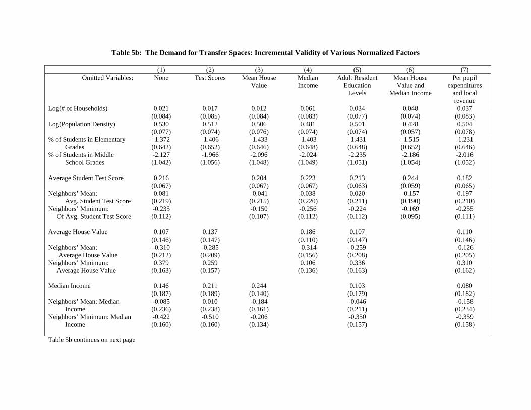
Table 5b: The Demand for Transfer Spaces: Incremental Validity of Various Normalized Factors

(1) (2) (3) (4) (5) (6) (7)Omitted Variables: None Test Scores Mean House

Value Median Income

Adult Resident Education

Levels

Mean House Value and

Median Income

Per pupil expenditures

and local revenue

Log(# of Households) 0.021 0.017 0.012 0.061 0.034 0.048 0.037 (0.084) (0.085) (0.084) (0.083) (0.077) (0.074) (0.083) Log(Population Density) 0.530 0.512 0.506 0.481 0.501 0.428 0.504 (0.077) (0.074) (0.076) (0.074) (0.074) (0.057) (0.078) % of Students in Elementary -1.372 -1.406 -1.433 -1.403 -1.431 -1.515 -1.231 Grades (0.642) (0.652) (0.646) (0.648) (0.648) (0.652) (0.646) % of Students in Middle -2.127 -1.966 -2.096 -2.024 -2.235 -2.186 -2.016 School Grades

(1.042) (1.056) (1.048) (1.049) (1.051) (1.054) (1.052)

Average Student Test Score 0.216 0.204 0.223 0.213 0.244 0.182 (0.067) (0.067) (0.067) (0.063) (0.059) (0.065) Neighbors’ Mean: 0.081 -0.041 0.038 0.020 -0.157 0.197 Avg. Student Test Score (0.219) (0.215) (0.220) (0.211) (0.190) (0.210) Neighbors’ Minimum: -0.235 -0.150 -0.256 -0.224 -0.169 -0.255 Of Avg. Student Test Score

(0.112) (0.107) (0.112) (0.112) (0.095) (0.111)

Average House Value 0.107 0.137 0.186 0.107 0.110 (0.146) (0.147) (0.110) (0.147) (0.146)Neighbors’ Mean: -0.310 -0.285 -0.314 -0.259 -0.126 Average House Value (0.212) (0.209) (0.156) (0.208) (0.205) Neighbors’ Minimum: 0.379 0.259 0.106 0.336 0.310 Average House Value

(0.163) (0.157) (0.136) (0.163) (0.162)

Median Income 0.146 0.211 0.244 0.103 0.080 (0.187) (0.189) (0.140) (0.179) (0.182)Neighbors’ Mean: Median -0.085 0.010 -0.184 -0.046 -0.158 Income (0.236) (0.238) (0.161) (0.211) (0.234) Neighbors’ Minimum: Median -0.422 -0.510 -0.206 -0.350 -0.359 Income

(0.160) (0.160) (0.134) (0.157) (0.158)

Table 5b continues on next page

% of Adults who are high -0.168 -0.270 -0.179 -0.154 -0.139 school dropouts (0.096) (0.093) (0.097) (0.096) (0.097) Neighbors’ Mean: % of adults -0.072 0.077 -0.077 -0.065 -0.180 who are high school dropouts (0.143) (0.131) (0.143) (0.142) (0.139) Neighbors’ Minimum: % of -0.158 -0.211 -0.121 -0.094 -0.079 adults who are high school dropouts

(0.122) (0.120) (0.121) (0.121) (0.121)

% of Adults with Bachelor’s -0.227 -0.211 -0.235 -0.224 -0.227 Degree (0.122) (0.120) (0.122) (0.118) (0.116) Neighbors’ Mean: % of Adults -0.180 -0.146 -0.168 -0.201 -0.084 with Bachelor’s Degree (0.135) (0.136) (0.132) (0.126) (0.130) Neighbors’ Minimum: % of 0.026 0.032 0.030 0.007 -0.065 Adults with Bachelor’s Degree

(0.092) (0.092) (0.091) (0.091) (0.084)

Public School Operating 0.150 0.098 0.134 0.138 0.128 0.103 Expenditures per Pupil (0.068) (0.065) (0.068) (0.068) (0.068) (0.067) Neighbors’ Mean: Public -0.166 -0.159 -0.157 -0.111 -0.156 -0.107 School Operating Expenditures per Pupil

(0.089) (0.080) (0.087) (0.088) (0.087) (0.082)

Neighbors’ Minimum: Public 0.002 0.010 0.020 0.018 -0.003 0.024 School Expenditures per Pupil

(0.057) (0.058) (0.057) (0.058) (0.057) (0.057)

Locally-funded Public School -0.142 -0.093 -0.127 -0.133 -0.168 -0.136 Expenditures per Pupil (0.073) (0.073) (0.073) (0.074) (0.072) (0.071) Neighbors’ Mean: Locally- 0.301 0.331 0.301 0.302 0.245 0.216 funded Public School Expenditures per Pupil

(0.104) (0.100) (0.098) (0.102) (0.100) (0.093)

Neighbors’ Minimum: -0.192 -0.233 -0.219 -0.227 -0.194 -0.220 Locally-funded Public School Expenditures per Pupil

(0.088) (0.089) (0.083) (0.087) (0.082) (0.076)

Constant 10.703 10.657 10.582 9.820 10.345 9.489 10.192 (1.479) (1.489) (1.487) (1.442) (1.432) (1.289) (1.492)Observations 329 329 329 329 329 329 329R-squared 0.538 0.517 0.527 0.523 0.512 0.493 0.512Note to Table 5b: All independent variables listed above have been converted to Z-scores.

37

Table 6: Estimated Coefficients of Additional Variables Measuring Districts’ Differentiated Services

Coefficient Standard Error % of Spending Spent on Vocational Ed.

District’s Own 0.107 0.051

Minimum Neighbor’s -0.039 0.057

Average Neighbors’ -0.005 0.056 % of Spending on Community Service

District’s Own 0.020 0.066

Minimum Neighbor’s 0.078 0.075

Average Neighbors’ -0.176 0.088 Indicator Variable for a Hockey Team Going to the State Finals Recently

-0.083 0.168

Indicator Variable for a Football Team Going to the State Finals Recently

-0.179 0.210

Notes to Table 6: All independent variables listed above have been converted to Z-scores, except for the hockey and football indicator variables. Regression also contains all of the independent variables included in other models (those included in column 1 of Table 5b). The R-squared of this regression equals .554.

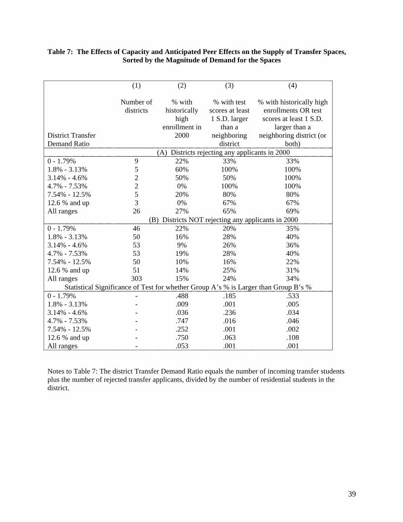
Table 7: The Effects of Capacity and Anticipated Peer Effects on the Supply of Transfer Spaces, Sorted by the Magnitude of Demand for the Spaces

District Transfer Demand Ratio

(1)

Number of districts

(2)

% with historically

high enrollment in

2000

(3)

% with test scores at least 1 S.D. larger

than a neighboring

district

(4)

% with historically high enrollments OR test scores at least 1 S.D.

larger than a neighboring district (or

both) (A) Districts rejecting any applicants in 2000 0 - 1.79% 9 22% 33% 33% 1.8% - 3.13% 5 60% 100% 100% 3.14% - 4.6% 2 50% 50% 100% 4.7% - 7.53% 2 0% 100% 100% 7.54% - 12.5% 5 20% 80% 80% 12.6 % and up 3 0% 67% 67% All ranges 26 27% 65% 69%

(B) Districts NOT rejecting any applicants in 2000 0 - 1.79% 46 22% 20% 35% 1.8% - 3.13% 50 16% 28% 40% 3.14% - 4.6% 53 9% 26% 36% 4.7% - 7.53% 53 19% 28% 40% 7.54% - 12.5% 50 10% 16% 22% 12.6 % and up 51 14% 25% 31% All ranges 303 15% 24% 34%

Statistical Significance of Test for whether Group A’s % is Larger than Group B’s % 0 - 1.79% - .488 .185 .533 1.8% - 3.13% - .009 .001 .005 3.14% - 4.6% - .036 .236 .034 4.7% - 7.53% - .747 .016 .046 7.54% - 12.5% - .252 .001 .002 12.6 % and up - .750 .063 .108 All ranges - .053 .001 .001 Notes to Table 7: The district Transfer Demand Ratio equals the number of incoming transfer students plus the number of rejected transfer applicants, divided by the number of residential students in the district.

39

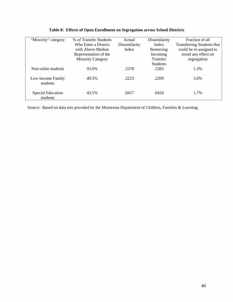
Table 8: Effects of Open Enrollment on Segregation across School Districts

“Minority” category % of Transfer Students Who Enter a District with Above Median

Representation of the Minority Category

Actual Dissimilarity

Index

Dissimilarity Index

Removing Incoming Transfer Students

Fraction of all Transferring Students that

could be re-assigned to avoid any effect on

segregation

Non-white students

93.0% .2378 .2383 1.3%

Low-income Family students

49.5% .2223 .2209 3.6%

Special Education students

43.5% .0417 .0424 1.7%

Source: Based on data sets provided by the Minnesota Department of Children, Families & Learning.

40