the surfpack software library for surrogate modeling of sparse

The Surfpack Software Library for Surrogate Modeling of Sparse Irregularly Spaced Multidimensional Data

Anthony A. Giunta1, Laura P. Swiler2, Shannon L. Brown2, and Michael S. Eldred3

Sandia National Laboratories∗, Albuquerque, NM USA

and

Mark D. Richards4 and Eric C. Cyr4 University of Illinois Urbana-Champaign, Urbana, IL USA

Surfpack is a general-purpose software library of multidimensional function approximation methods for applications such as data visualization, data mining, sensitivity analysis, uncertainty quantification, and numerical optimization. Surfpack is primarily intended for use on sparse, irregularly-spaced, n-dimensional data sets where classical function approximation methods are not applicable. Surfpack is under development at Sandia National Laboratories, with a public release of Surfpack version 1.0 in August 2006. This paper provides an overview of Surfpack’s function approximation methods along with some of its software design attributes. In addition, this paper provides some simple examples to illustrate the utility of Surfpack for data trend analysis, data visualization, and optimization.

1. Introduction Surrogate models based on function approximations (also known as metamodels, response surface approximations, hypersurfaces, and curve fits) are commonly used to capture, both qualitatively and quantitatively, the underlying trends in a discrete set of data. In cases where the data points are regularly spaced, there are a variety of mathematical techniques for creating function approximations (e.g., various types of orthogonal polynomials). However, in cases where there are few data points and/or when the data points are irregularly spaced, these classical techniques are not applicable. This situation often occurs in engineering and scientific applications when data points are expensive to obtain. For example, a geologist might have a small number of Earth core samples from a set of irregularly-spaced drill sites in a region of interest. The geologist could then use a function approximation method to create a surrogate model to “map” some measured quantity (e.g., moisture content) over the region of interest, in order to estimate the best location for the next drill site. Similar uses for surrogate models arise in data mining, numerical optimization, parameter sensitivity studies, and uncertainty quantification applications (cf. Jones et al. 1998, Giunta et al. 2006, Simpson et al. 2001,). In an effort to better understand the strengths and weaknesses of surrogate models, there have been numerous studies investigating the function approximation types and/or the data sampling methods used in constructing surrogate models (cf. Jin et al. 2000, Simpson et al. 2002, and Swiler et al. 2006). The Surfpack software tool described in this paper is intended to facilitate such studies by providing the engineering and scientific community with a publicly-available, easy-to-use tool for creating surrogate models from sparse multidimensional data sets. The Surfpack library of surrogate modeling methods has been under development at Sandia National 1 AIAA Senior Member, Validation and Uncertainty Quantification Dept., Corresponding Author, Postal Address: Sandia National Laboratories, P.O. Box 5800, Mail Stop 0828, Albuquerque, NM 87185-0828, USA. 2 AIAA Member, Optimization and Uncertainty Estimation Dept. 3 AIAA Associate Fellow, Optimization and Uncertainty Estimation Dept. 4 Graduate Student, Department of Computer Science. ∗ Sandia is a multiprogram laboratory operated by Sandia Corporation, a Lockheed Martin Company, for the United States Department of Energy’s National Nuclear Security Administration under Contract DE-AC04-94AL85000.

American Institute of Aeronautics and Astronautics

1

Laboratories since 2002. In August 2006 it was released to the public under the terms of the GNU General Public License (GPL). This release under GNU GPL is targeted at users in the engineering and scientific community with the intent that (a) Surfpack gets tested on many diverse data modeling and analysis projects, and (b) Surfpack grows in capability as users add their own function approximation methods to the Surfpack library. Surfpack will be supported by a small development team at Sandia National Labs which will maintain and upgrade the software as needed, and will provide limited user support. In theory, there are no fixed limits in Surfpack with respect to the number of data points or the dimension of the parameter space. However, in practice, Surfpack is generally targeted at applications with on the order of 10s to 100s of data points, and 10s of dimensions. The remainder of this paper is arranged as follows: Section 2 covers some aspects of the Surfpack software design, Section 3 describes the function approximation methods in Surfpack, and Section 4 addresses the function approximation error measures. Section 5 contains three simple Surfpack examples. Sections 6 and 7 provide some final remarks on the current status and future directions of the Surfpack project.

2. Software Design of Surfpack The Surfpack software is written in a combination of C++ and FORTRAN77. The C++ portion of Surfpack provides the primary data management and user interface capabilities, while FORTRAN77 is used for some of the surrogate model construction calculations. The design of Surfpack allows for the easy addition of new surface fitting function types, and our intent is for Surfpack to gain new capabilities as members of the Surfpack user community add in their favorite surface fitting methods. The Surfpack software package operates in both a stand-alone mode and in a library mode. In the stand-alone mode, which is the focus of this paper, the user provides two input files to Surfpack that contain a set of input commands along with the user’s data. Surfpack is then executed and it outputs data files back to the user. In the library mode, Surfpack can be linked into a user’s C++ program to provide the user with more control over the calculations and data manipulations performed by Surfpack. The intended use of Surfpack is as one of a suite of tools that a user would apply in an engineering or scientific data exploration study. That is, the user would employ other tools to generate the data sets (e.g., via computer simulations or laboratory measurements), and then would apply Surfpack to gain both qualitative and quantitative insights into the data trends. A detailed statistical analysis of the user’s data is not handled in Surfpack, as there are numerous existing software packages that provide such capabilities. At this time, Surfpack does not provide a graphical user interface for either input data preparation or output data visualization. Given that Surfpack can generate output data on a regular Cartesian grid of points, its output files can be readily imported into many graphics and plotting packages (e.g., Microsoft Excel, gnuplot, Mathematica, Matlab, Tecplot). See below for examples of such applications.

3. Function Approximation Methods in Surfpack

3.1 Low-Order Polynomials Linear, quadratic, and cubic polynomial models are available in Surfpack. The form of the n-dimensional linear polynomial model is:

( ) 01

ˆn

i ii

f x c c x=

= +∑ , (1)

the form of the quadratic polynomial model is:

( ) 01 1

ˆn n n

i i ij i ji i j i

f x c c x c x x= = ≥

= + +∑ ∑∑ , (2)

and the form of the cubic polynomial model is:


2

( ) 01 1 1

ˆn n n n n n

i i ij i j ijk i j ki i j i i j i k j

f x c c x c x x c x x x= = ≥ = ≥ ≥

= + + +∑ ∑∑ ∑∑∑ . (3)

In all of the polynomial models, ( )f̂ x is the predicted response of the polynomial model; the xi, xj, xk terms are the components of the n-dimensional design parameter values; the c0 , ci , cij , cijk terms are the polynomial coefficients, and n is the number of design parameters. The number of coefficients, nc, depends on the order of the polynomial model and the number of design parameters. For the linear polynomial: nc = n + 1, for the quadratic polynomial: nc = (n + 1)(n + 2)/2, and for the cubic polynomial: nc = (n3 + 6n2 + 11n + 6)/6. There must be at least nc data samples in order to form a fully determined system of linear equations. Surfpack employs a standard least-squares approach using subroutines from the LAPACK software library (Anderson 1999) to solve the linear system for the unknown coefficients. The utility of the polynomial models stems from two sources: (a) over a small portion of the parameter space, a low-order polynomial model is often an accurate approximation to the true data trends, and (b) the least-squares procedure serves to smooth out noise in the data. However, a polynomial surface fit may not be the best choice for modeling data trends over an entire parameter space, unless it is known a priori that the true data trends are approximately linear, quadratic, or cubic.

3.2 Kriging Interpolation Kriging interpolation techniques were originally developed in the geostatistics and spatial statistics communities to produce maps of underground geologic deposits based on samples obtained at widely and irregularly spaced borehole sites (Cressie 1991). The basic notion that underpins kriging is that the sample response values exhibit spatial correlation, with response values modeled via a Gaussian process around each sample location (i.e. samples taken close together are likely to have highly correlated response values, whereas samples taken far apart are unlikely to have highly correlated response values). Kriging methods have wide utility due to their ability to accommodate irregularly spaced data, their ability to model general surfaces that have many peaks and valleys, and their exact interpolation of the given sample response values. The specific form of the kriging model used in this study is described in Giunta and Watson (1998) and Romero, et al. (2004), and it is based on the work of Koehler and Owen (1996). The form of the kriging model is

( ) ( ) 1ˆ ˆ ( {1Tf x r x R fβ −= + − ˆ })β , (4)

where β̂ is the generalized least squares estimate of the mean response; r(x) is an N µ 1 vector of correlations between the current point x and all N sample sites in parameter space; R is the N µ N correlation matrix of all N sample sites; f is the vector of N sample site response values; and {1} is an N µ 1 vector with all values set to unity. The terms in the correlation vector and matrix are computed using a Gaussian correlation function. The ith term in r(x) is given by

2( )

1exp n i

i k kkr xθ

=⎡= − −⎢⎣ ⎦∑ kx ⎤

⎥ , (5)

and, similarly, the i,jth term in R is given by

2( ) ( ), 1

exp n i ji j k k kk

R xθ=

x⎡ ⎤= − −⎢ ⎥⎣ ⎦∑ , (6)

where n is the dimension of the parameter space; k is the index on the dimension of the parameter space; i = 1,…,N; j = 1,…,N; and q is the n µ 1 vector of correlation parameters. In the most general approach to kriging, the values of q are computed using maximum likelihood estimation. However, finding optimal q values can be problematic, as it requires an iterative search scheme that can fail to converge. The kriging interpolation method is prone to ill-conditioning in the correlation matrix R as the number of sample points increases. This occurs because of the distance measure that is computed in Equation (6). As the distance between any two sample points i and j decreases, then the ith and jth rows in matrix R become linearly


3

dependent, and in the limit where the points are the same, the matrix R becomes singular. Thus, this basic kriging method works well for a sparse set of sample points in an n-dimensional parameter space, but as the number of samples increases (and the inter-point distances decrease), the basic kriging method becomes numerically unstable.

3.3 Multivariate Adaptive Regression Splines The multivariate adaptive regression splines (MARS) function approximation method (Friedman 1991) is based on a complex, recursive partitioning algorithm involving truncated power spline basis functions. The form of the MARS model is:

( ) ( ) ( )1 2

1 1

ˆ , ...M M

o m m i m m i jm m

f x a a B x a B x x= =

= + + +∑ ∑ (7)

where the Bm terms are the basis functions, the am terms are the coefficients of the basis functions, M1 is the number of one-parameter basis functions, and M2 is the number of two-parameter basis functions. The MARS software allows the user to select either linear or cubic spline basis functions. The regression aspect of the MARS algorithm involves a forward/backward stepping process to adaptively add/remove spline basis functions from the model. This regression process generates the ao and am terms in Equation (7). The resulting MARS surrogate model is a C2-continuous function of piecewise cubic splines (or a C1-continuous function of piecewise linear splines), but it will not exactly interpolate the data points that were used in calculating the coefficients. Thus, like polynomial regression, MARS has the ability to create smooth approximations to noisy data. Unlike kriging, MARS appears to have no upper limit on the number of samples that can be used in the function approximation process. Note: As of August 2006 there are some software bugs in the interface between the MARS code and the main Surfpack code. We suggest that users exercise caution in using the MARS method within Surfpack until further testing with MARS/Surfpack has been performed by the Surfpack development team. For this reason, the Surfpack examples contained in this paper do not exercise the MARS function approximation approach.

3.4 Artificial Neural Networks The artificial neural network (ANN) surrogate modeling method in Surfpack employs a stochastic layered perceptron (SLP) network based on the direct training approach of Zimmerman (1996). The SLP ANN method is designed to have a lower training cost than traditional ANNs as it uses fixed-value weights on some of the links within the network. That is, only a portion of the network weights must be computed in the ANN training process. While this approach offers a lower training cost than traditional ANNs, it sacrifices some of the modeling flexibility offered by traditional ANNs. The functional form of the SLP ANN model is:

( ) ( )( )0 0 1 1ˆ tanh tanhf x xA Aθ θ= + + , (8)

where x is the current point in n-dimensional parameter space, and the terms A0, q0, A1, q1 are the matrices and vectors that correspond to the neuron weights and offset values in the ANN model. These terms are computed during the ANN training process, and are analogous to the polynomial coefficients in a polynomial function approximation. This ANN method employs a singular value decomposition method to solve for the weight and offset terms in the model. The SLP ANN is a non parametric surface fitting method. Thus, along with kriging and MARS, it can be used to model data trends that have slope discontinuities as well as multiple maxima and minima. However, unlike kriging, the ANN surface is not guaranteed to exactly match the response values of the data points from which it was constructed. Thus, this ANN method provides some data smoothing similar to that provided by the low-order polynomials. Note: The authors have found that this particular SLP ANN method exhibits erratic modeling accuracy in some applications (see below). Users of this SLP ANN method should exercise caution.


4

4. Function Approximation Error Measures Surfpack provides various measures of function approximation accuracy. The examples shown in this study employ three of these measures: (a) the R2 coefficient of determination, (b) the root mean squared (RMS) error, and (c) the predicted error sum of squares (PRESS). The R2 coefficient of determination is used to assess the accuracy of polynomial regression models. It measures the amount of variability in the user-supplied f(x) data that is captured by the polynomial regression model ˆ ( )f x . The R2 value is computed as

( )( )

2

2 1

2

1

ˆN

iiN

ii

f fR

f f

=

=

−=

−

∑

∑, (9)

where f is the mean of the f(x) values, f̂ is the polynomial function approximation prediction at each of the data points, and N is the number of data points. The RMS error quantifies the amount of residual error between the f-value data and the f-value predictions at the N data points. It is valid for all of the function approximation methods in Surfpack. RMS error is computed as

( )2

1

ˆN

i ii

f fRMS

N=

−=∑

. (10)

Note that the RMS error measure is, theoretically, zero for the kriging method since it exactly interpolates the supplied f-value data. However, in practice, the RMS error is nonzero (but still very small) due to the numerical methods used to construct the kriging model. So, because the kriging method performs data interpolation, and the other surrogate methods in this study perform data smoothing, the RMS error measure is not always a fair comparison of accuracy among the methods. The PRESS error measure (Allen 1971, 1974) is a type of cross-validation procedure in that it assesses the accuracy of the function approximation when individual data points are omitted from the data used to create the approximation. PRESS is computed as

(2

( )1

ˆN

i ii

PRESS f f=

= −∑ ) , (11)

where ( )

ˆif is the ith function approximation model obtained by omitting the ith data point from the data set when

constructing the model. This PRESS measure is often referred to as a “leave one point out” cross-validation method. Other “leave k points out” PRESS variants have been explored in the statistics literature, but are not included in Surfpack at this time.

5. Applications of Surfpack This section covers three examples of Surfpack on a: (a) set of one-dimensional data, (b) set of two-dimensional data, and (c) set of four-dimensional data. The one- and two-dimensional examples are shown to illustrate Surfpack’s basic capabilities. The four-dimensional example showcases Surfpack’s primary utility which is the generation of multidimensional function approximations, along with the capability to easily generate two- and three-dimensional data sets for visualization purposes.


5

5.1 Example: One-Dimensional Data Table 1 lists the data points used in this example which were obtained from a series of expensive computational fluid dynamics (CFD) simulations. Here, x is the independent parameter which corresponds to an input to the CFD simulation, and f is the dependent parameter which corresponds to a force coefficient value computed in the CFD simulation. Surfpack is used to approximate the trends of f-vs.-x, and to predict f(x) at untried values of x. Appendices A and B list the Surfpack command and data input files, respectively, and Appendix C lists the Surfpack data output file. In this example, Surfpack takes as input the data listed in Appendix B, creates five different function approximations to this data (three low-order polynomial models, a kriging model, and a neural network model), and then outputs f(x) values for 27 evenly spaced points over the range -4.0 § x § 1.2. Surfpack also produces error measures for each function approximation: R2, RMS, and PRESS. These error measures are listed in Table 2. The plots in Figure 1(a)-(f) show the original data points, along with Surfpack-generated trends using each of the five function approximation types specified in the Surfpack command input file. The low-order polynomial approximations in Figure 1(b), (c), and (d) illustrate the data smoothing properties of least-squares regression methods for overdetermined linear systems. (Note: Figure 1(c) and Figure 1(d) are very similar, but not identical.) Figure 1(e) shows the interpolating properties of the kriging method, and Figure 1(f) shows the nonparametric smoothing properties of the SLP neural network method. Of course, there is no clear distinction of a “best” approximation, since what is “best” is relative to the needs of the user. In some instances the user will require data smoothing methods, whereas in other instances the user will require data interpolation methods. A more quantitative, but still relative, assessment of function approximation accuracy is provided by the error measure data in Table 2. These error measures provide information on the amount of data variability that is captured by the different function approximation models. The R2 values show that all three polynomial models provide reasonable fits to the data, with the 2nd and 3rd order polynomials providing nearly identical accuracy. The RMS error measures show that the low-order polynomials and the ANN method provide about the same quality of fit to the data with respect to residual error. As expected, the RMS error for kriging is nearly zero. The PRESS measure provides the clearest comparison among the different function approximation models. In this case, the PRESS measures indicate that the kriging model, neural network model, and 2nd order polynomial model have comparable accuracy in predicting missing f-values. Also, the PRESS measures indicate that these three models are slightly more accurate than the 1st and 3rd order polynomial models.

5.2 Example: Two-Dimensional Data The two-dimensional Surfpack example was created using the Matlab “peaks” function

( ) ( ) ( )( ) ( ) ( )( )2 22 22 21 2 2 11 21 12 3 51

1 2 1 1 21, 3 1 10

5 3x x x xx xxf x x x e x x e e

− − + − − +− −⎛ ⎞ ⎛ ⎞= − − − − − ⎜ ⎟⎜ ⎟⎝ ⎠⎝ ⎠

. (12)

A three-dimensional plot of f(x1,x2) is shown in Figure 2 over the range -3.0 § x1, x2 § 3.0. A two-dimensional contour plot of this function along with the locations of 20 randomly generated (x1,x2) sample sites is shown in Figure 3. The x- and f-values for these 20 sample sites are listed in Table 3. Appendices D and E list the Surfpack command and data input files, respectively. Note that the commands in Appendix D specify that Surfpack will produce f(x1,x2) predictions on a 13µ13 grid of points in (x1,x2) over the range -3.0 § x1, x2 § 3.0. As in the one-dimensional example, Surfpack will generate 1st, 2nd, and 3rd order polynomial models, a kriging interpolation model, and a neural network model for the data. Appendix F lists the (abbreviated) output data produced by Surfpack. These data were used to generate the following contour plots: 1st order polynomial approximation (Figure 4), 2nd order polynomial approximation (Figure 5), 3rd order polynomial approximation (Figure 6), kriging approximation (Figure 7), and neural network approximation (Figure 8). Qualitatively, visual comparisons of these figures with Figure 3 show that the low-order polynomials are poor approximations to the trends in the peaks function, whereas the kriging interpolation captures the major features of the peaks function. The neural network approximation is alarmingly poor. Additional studies (not presented here) are underway to determine whether this poor performance is due to software bugs or due to inherent limitations of the SLP ANN algorithm.


6

Quantitative measures of function approximation accuracy for this example are listed in Table 4. The R2 values for the polynomial models confirm the visual trends, i.e., that even the 3rd order polynomial doesn’t capture much of the variability in the 20 data samples. The RMS error values are as expected, given the poor fitting of the polynomials and the neural network model. The PRESS results are the most interesting. Note that the PRESS measure for the 1st order polynomial is lower than the PRESS measure for the kriging model. However, most users would prefer the kriging model over the 1st order polynomial given the differences between Figure 4 and Figure 7 versus the original peaks function (Figure 3). Thus, error measures alone do not always provide sufficient information by which to choose a “best” function approximation.

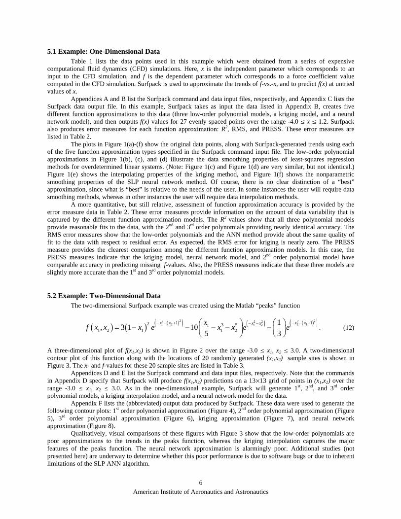
5.3 Example: Four-Dimensional Data This four-dimensional example is drawn from a real-world application of Surfpack on an engineering analysis problem. This example has four independent parameters, (x1, x2, x3, x4), and a single dependent response value. There are 42 samples in this four-dimensional parameter space, which were generated using a combination of statistical design of experiments methods and random sampling methods. Table 5 provides a list of these data points. The objective of this study was to find the point (or region) in the four-dimensional parameter space where the response value was minimized. Appendices G and H list the Surfpack command and data input files, respectively, for this example. This example uses the same five function approximation methods, and the same three error measures, as in the one- and two-dimensional examples. Note that the Surfpack command input file in Appendix G contains instructions to produce function approximation data on an 11µ11µ11µ1 grid of points in (x1, x2, x3, x4) space. That is, x1-x3 are varied between their respective lower and upper bounds, while x4 is held constant (x4 = 0.7). This was done to permit visualization of the function approximation data. Appendix I lists a portion of the output from Surfpack, with columns 1-4 corresponding to x1- x4 and column 5 corresponding to the kriging interpolation model predictions (note that columns for the low-order polynomial and ANN predictions generated by Surfpack were omitted for readability). Table 6 lists the R2, RMS error, and PRESS measures for this example. While the R2 values and RMS error values appear reasonable, the PRESS calculation for the 3rd order polynomial uncovered an unexpected problem with the PRESS metric. In this particular case, the PRESS calculation process generated a rank-deficient linear system of equations which caused a large spike in the PRESS value. This sensitivity of the 3rd order polynomial to the loss of a single data point forced us to question the accuracy of the 3rd order polynomial approximation for this application. Thus, only the kriging interpolation model was used for subsequent studies. These results are discussed below. Figure 9 shows the locations of the 42 samples in the four-dimensional parameter space. Note that not all 42 points are visible in this figure due to the projection into a three-dimensional space for visualization. Figure 10 shows the Surfpack-generated (via kriging) response function contours along a portion of the external boundary of the four-dimensional parameter space. By plotting two-dimensional “slices” of this block of data, it is possible to see the response function contours in the interior of the parameter space. This is shown in Figure 11. The sample point locations (dark spheres) are also shown in this figure to demonstrate how the kriging interpolation method is providing response predictions in between the samples. (Note: the spheres are dark colored to aid in visualization. The dark color does not indicate a lack-of-fit between the original data and the kriging model.) For the engineering application that supplied the 42 data samples, the Surfpack results shown in Figure 11 clearly identified the region of the parameter space where the objective function was minimized (i.e., the green-shaded contour portions of the parameter space). Thus, by inspection, the optimal x1-x4 values were identified. [Note: additional runs of the simulation code that produced the f(x) values confirmed, qualitatively, that the optimal x1-x4 were acceptable.] Had this been a higher-dimensional problem, it would have been relatively easy to identify the optimal x-parameter values by either (a) brute-force interrogation of the parameter space via Surfpack, or (b) formal optimization via linking a numerical optimization software package to Surfpack.

5.4 Surfpack Execution Syntax The three Surfpack examples discussed above have the same basic execution syntax, which on computers running a Linux/Unix-type operating system is: surfpack input_commands.spk


7

where “surfpack” is the name of the Surfpack executable file, and “input_commands.spk” is the name of the Surfpack command input file. A key item to note is the “.spk” extension on the Surfpack command input file. This “.spk” extension is required. Also, note that this execution syntax will result in the display of the error measure data to the user’s computer terminal. This output can be redirected to a file using the usual Linux/Unix file redirection command, e.g., by appending the command “ > output_file” to the Surfpack execution command given above. Another important Surfpack syntax note is the required use of the “.spd” extension on all Surfpack input and output data files. Surfpack will generate an error message if these file name extension rules are not followed. As an example, listed below is the Surfpack execution syntax for the one-dimensional example problem discussed above, with its corresponding input and output files listed in Appendices A, B, and C: surfpack engineering_1d.spk > error_output Here, “engingeering_1d.spk” is the file in Appendix A. The commands in “engineering_1d.spk” tell Surfpack to read in a file named “engineering_1d.spd” (see Appendix B) and to write output data to a file named “test_data.spd” (see Appendix C). The R2, RMS, and PRESS error measures computed by Surfpack are written to the file named “error_output” (see Table 2). Note that all Surfpack input and output files are written in plain ASCII text format. The use of some file editing software packages (e.g., Microsoft Word) can unintentionally introduce hidden end-of-line characters that Surfpack cannot read. These hidden characters can be removed using commonly-available Linux operating system tools such as “dos2unix” which converts Microsoft text files into ASCII text files.

6. Surfpack Future Directions While currently Surfpack is primarily a software development project intended to support engineering analysis and design applications, we anticipate using Surfpack for future research studies. These potential research areas include development of (a) new function approximation methods based on radial basis functions and on Gaussian process models, (b) new surrogate-based uncertainty quantification methods using PRESS-type error estimates, and (c) “best” surrogate model selection methods using decision theory techniques. Clearly, there are many interesting research topics to explore with Surfpack. More information on Surfpack can be obtained at the following web site http://endo.sandia.gov/surfpack This web site has links to the Surfpack executable files (for different computer platforms), Surfpack source code files, and the Surfpack User’s Manual. The manual contains instructions for installing and using Surfpack. Links are provided on this website to contact the Surfpack development team via email.

7. Summary This paper describes some of the attributes of the Surfpack software package in an attempt to demonstrate its utility to the engineering and scientific community. This text provides an overview of the Surfpack software architecture and briefly covers some of the mathematics of the function approximation methods in Surfpack. Three examples are shown to illustrate Surfpack’s capabilities. The August 2006 public release of Surfpack will provide the engineering and scientific community with an easy-to-use library of surrogate models for use in applications such as optimization, uncertainty quantification, sensitivity analysis, and data mining. The open-source availability of the Surfpack software, and its object-oriented C++ software design, should permit the rapid addition of new surrogate model types as users can readily implement their own favorite surrogate models within Surfpack. As per the requirements of the GNU General Public License, future versions of Surfpack with user-supplied surrogate models will be freely available to the engineering and scientific community.


8

References

Allen, D. M., “Mean Square Error of Prediction as a Criterion for Selecting Variables,” Technometrics, Vol. 13, 1971, pp. 469-475.

Allen, D. M., “The Relationship Between Variable Selection and Data Augmentation and a Method for Prediction,” Technometrics, Vol. 16, 1974, pp. 125-127.

Anderson, E., Bai, Z., Bischof, C., Blackford, S., Demmel, J., Dongarra, J., Du Croz, J., Greenbaum, A., Hammarling, S., McKenney, A., and Sorensen, D., LAPACK Users’ Guide, 3rd Edition, SIAM, Philadelphia, PA, 1999.

Cressie, N., Statistics of Spatial Data, John Wiley and Sons, New York, 1991.

Friedman, J. H., “Multivariate Adaptive Regression Splines,” Annals of Statistics, Vol. 19, No. 1, 1991, pp. 1-141.

Giunta, A. A., and Watson, L. T., “A comparison of approximation modeling techniques: polynomial versus interpolating models,” paper AIAA 98-4758 in Proceedings of the 7th AIAA/USAF/NASA/ISSMO Symposium on Multidisciplinary Analysis and Optimization, St. Louis, MO, 1998, pp. 392-404.

Giunta, A. A., McFarland, J. M., Swiler, L. P., and Eldred, M. S., "The Promise and Peril of Uncertainty Quantification using Response Surface Approximations," Structure & Infrastructure Engineering: Maintenance, Management, Life-Cycle Design & Performance, special issue on Uncertainty Quantification and Design under Uncertainty of Aerospace Systems, Vol. 2, Nos. 3-4, Sept.-Dec. 2006, pp. 175-189.

Jin, R., Chen, W., and Simpson, T. W., “Comparative Studies of Metamodeling Techniques Under Multiple Modeling Criteria,” paper AIAA-2000-4801 in Proceedings of the 8th AIAA/USAF/NASA/ISSMO Symposium on Multidisciplinary Analysis and Optimization, Long Beach, CA, 2000.

Jones, D. R., Schonlau, M., and Welch, W. J., “Efficient Global Optimization of Expensive Black-Box Functions,” Journal of Global Optimization, Vol. 13, No. 4, 1998, pp. 455-492.

Koehler, J. R., and Owen, A. B., “Computer experiments,” in Handbook of Statistics, 13, edited by S. Ghosh and C.R. Rao, Elsevier Science, 1996, pp. 261-308.

Romero, V. J., Swiler, L. P., and Giunta, A. A., “Construction of response surfaces based on progressive-lattice-sampling experimental designs,” Structural Safety, Vol. 26, No. 2, 2004, pp. 201-219.

Simpson, T. W., Mauery, T. M., Korte, J. J., and Mistree, F., “Kriging Models for Global Approximation in Simulation-Based Multidisciplinary Design Optimization,” AIAA Journal, Vol. 39, No. 12, 2001, pp. 2233-2241.

Simpson, T., Dennis, L., and Chen, W., “Sampling Strategies for Computer Experiments: Design and Analysis” Journal of International Journal of Reliability and Application, Vol. 2, No. 3, 2002, pp. 209-240.

Swiler, L. P., Slepoy R., and Giunta, A. A., “Evaluation of Sampling Methods in Constructing Response Surface Approximations,” paper AIAA-2006-1827 in Proceedings of the 47th AIAA/ASME/ASCE/AHS/ASC Structures, Structural Dynamics, and Materials Conference (2nd AIAA Multidisciplinary Design Optimization Specialist Conference), Newport, Rhode Island, 2006.

Zimmerman, D. C., “Genetic Algorithms for Navigating Expensive and Complex Design Spaces,” Final Report for Sandia National Laboratories contract AO-7736 CA 02, Sept. 1996.


9

Table 1. Data for the one-dimensional Surfpack example.

1.000.40

-0.20-0.80-1.40-2.00-2.60-3.20-3.80

x0.0013990.0021190.0002230.0002650.001145

-0.001141-0.002576-0.004553-0.005357

f

Table 2. Error measures for the different function approximations used on the one-dimensional example data: poly1 = 1st order polynomial, poly2 = 2nd order polynomial, poly3 = 3rd order polynomial, kriging = kriging interpolation,

ann = artificial neural network.

Error Measure and Approximation Method Result

0.850133 rsquared for poly1_eng:0.936443 rsquared for poly2_eng:0.936467 rsquared for poly3_eng:

0.000976474 RMS for poly1_eng:0.0006359 RMS for poly2_eng:0.000635781 RMS for poly3_eng:

RMS for kriging_eng : 2.14942e-18 0.000606223 RMS for ann_eng :

press for poly1_eng: 1.449e-5 press for poly2_eng: 7.394e-6 press for poly3_eng: 1.389e-5 press for kriging_eng : 5.535e-6 press for ann_eng : 6.277e-6


10

Table 3. Data for the two-dimensional Surfpack example.

1.096248430.83041563-0.5581232-0.73820822.63411796-2.35162981.51688767-2.7054121-0.24470160.05541495-1.2037754-1.5782337-1.93072252.3650993

0.45253993-1.10169632.847599181.31288841-2.65530151.91541045

x1-2.75270992.50714772-1.0447864-1.52036991.64582071-1.8914058-0.85745360.013730081.427743850.644981042.31058493-0.15971290.5617785

2.70111692-1.25023861.89351392-2.6275485-0.4530109-2.231739

0.97756262

x2-0.24117670.929606952.01766673-0.83670480.019274450.018154131.38611238-0.13602317.3066754

0.768382920.72403075

-2.336954-1.23299960.00395092-4.53071211.90473674-0.00009232.916615650.003093160.74057462

f(x1,x2)

Table 4. Error measures for the different function approximations used on the two-dimensional example data.

Error Measure and Approximation Method Result rsquared for poly1_peaks: 0.0880982 rsquared for poly2_peaks: 0.121961 rsquared for poly3_peaks: 0.338186 RMS for poly1_peaks: 2.11262 RMS for poly2_peaks: 2.07303 RMS for poly3_peaks: 1.79977 RMS for kriging_peaks: 6.70656e-16 RMS for ann_peaks: 1.86851 press for poly1_peaks: 109.994 press for poly2_peaks: 133.671 press for poly3_peaks: 291.638 press for kriging_peaks: 120.448 press for ann_peaks: 127.502


11

Table 5. Data for the four-dimensional Surfpack example.

1.200.500.500.850.850.500.500.851.200.851.201.201.200.500.500.850.851.200.501.201.200.850.501.200.501.000.900.950.851.301.150.801.001.251.401.351.201.501.451.051.100.72

x11.504.503.001.503.001.504.503.004.503.001.504.501.501.501.503.004.501.504.504.503.003.004.504.501.503.002.863.502.712.502.573.292.643.433.363.002.933.212.793.143.073.03

x20.701.000.850.850.851.001.000.701.001.000.700.701.001.000.700.850.851.000.700.700.850.850.701.000.700.800.970.960.890.840.930.870.800.860.990.831.000.900.940.810.910.82

x30.701.000.850.850.851.000.700.850.700.851.001.000.700.701.000.700.851.000.700.700.851.001.001.000.700.800.700.700.700.700.700.700.700.700.700.700.700.700.700.700.700.70

x412.9015.409.90

15.508.30

21.5015.407.409.109.30

12.009.308.708.20

24.006.309.207.20

15.408.308.609.50

15.508.70

24.808.808.31

10.728.047.847.368.427.658.019.009.218.298.508.608.557.728.29

f(x)


12

Table 6. Error measures for the different function approximations used on the four-dimensional example data.

Error Measure and Approximation Method Result rsquared for poly1_4d: 0.461845 rsquared for poly2_4d: 0.831277 rsquared for poly3_4d: 0.981871 RMS for poly1_4d: 3.18337 RMS for poly2_4d: 1.78246 RMS for poly3_4d: 0.584271 RMS for kriging_4d: 2.97775e-14 RMS for ann_4d: 0.899148 press for poly1_4d: 602.087 press for poly2_4d: 655.929 press for poly3_4d: 1.21e+23 (see note in text) press for kriging_4d: 707.487 press for ann_4d: 1636.8


13

Figure 1. Plots of the one-dimensional Surfpack example showing (a) the original data, (b) a 1st order polynomial

model, (c) a 2nd order polynomial model, (d) a 3rd order polynomial model, (e) a kriging interpolation model, and (f) a neural network model.


14

Figure 2. A three-dimensional view of the Matlab peaks function.

Figure 3. A contour plot of the Matlab peaks function showing the locations of the 20 random samples (stars) used

to provide data to Surfpack.


15

-3

-2

-1

0

1

2

3

x2

-3 -2 -1 0 1 2 3

x1

Legend

poly1

<= -6.000

<= -4.500

<= -3.000

<= -1.500

<= 0.000

<= 1.500

<= 3.000

<= 4.500

<= 6.000

> 6.000

Figure 4. Contours for a Surfpack-generated 1st order polynomial approximation based on the 20 data points (stars) sampled from the Matlab Peaks function.

-3

-2

-1

0

1

2

3

x2

-3 -2 -1 0 1 2 3

x1

Legend

poly2

<= -6.000

<= -4.500

<= -3.000

<= -1.500

<= 0.000

<= 1.500

<= 3.000

<= 4.500

<= 6.000

> 6.000

Figure 5. Contours for a Surfpack-generated 2nd order polynomial approximation based on the 20 data points (stars) sampled from the Matlab Peaks function.


16

-3

-2

-1

0

1

2

3

x2

-3 -2 -1 0 1 2 3

x1

Legend

poly3

<= -6.000

<= -4.500

<= -3.000

<= -1.500

<= 0.000

<= 1.500

<= 3.000

<= 4.500

<= 6.000

> 6.000

Figure 6. Contours for a Surfpack-generated 3rd order polynomial approximation based on the 20 data points (stars) sampled from the Matlab Peaks function.

-3

-2

-1

0

1

2

3

x2

-3 -2 -1 0 1 2 3

x1

Legend

kriging

<= -6.000

<= -4.500

<= -3.000

<= -1.500

<= 0.000

<= 1.500

<= 3.000

<= 4.500

<= 6.000

> 6.000

Figure 7. Contours for a Surfpack-generated kriging interpolation based on the 20 data points (stars) sampled from the Matlab Peaks function.


17

-3

-2

-1

0

1

2

3

x2

-3 -2 -1 0 1 2 3

x1

Legend

ann

<= -6.000

<= -4.500

<= -3.000

<= -1.500

<= 0.000

<= 1.500

<= 3.000

<= 4.500

<= 6.000

> 6.000

Figure 8. Contours for a Surfpack-generated neural network approximation based on the 20 data points (stars) sampled from the Matlab Peaks function.

Figure 9. The locations of the 42 samples in the four-dimensional example (projected down to a three-dimensional

space for visualization).


18

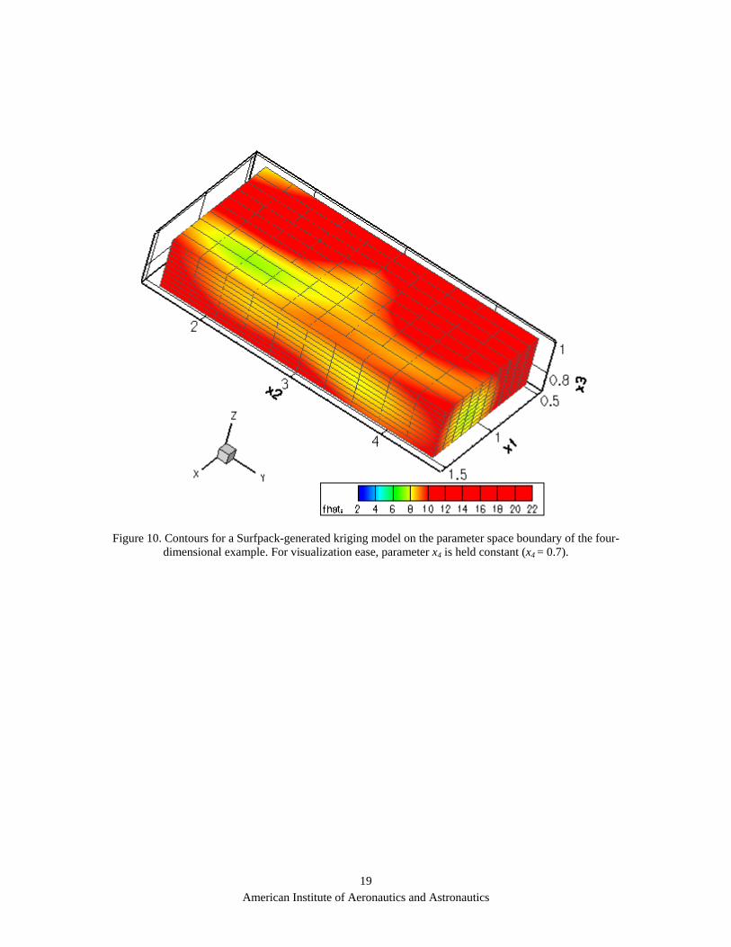
Figure 10. Contours for a Surfpack-generated kriging model on the parameter space boundary of the four-

dimensional example. For visualization ease, parameter x4 is held constant (x4 = 0.7).


19

Figure 11. Contour “slices” through the four-dimensional data set generated via Surfpack’s kriging interpolation

method. The spheres are the 42 sample points (note: sphere color intentionally does not match the contour color to aid in visualization). The green color contours indicate regions of interest where the response function “fhat” (see

legend) has low values.


20

Appendix A. The Surfpack command input file named “engineering_1d.spk” for the one-dimensional example. # Read in data Load[name = eng_1d, file = 'engineering_1d.spd', n_predictors = 1, n_responses = 1] # Create a test set with 27 points, evenly spaced .2 apart CreateAxes[name = ax_1d, bounds = '-4 1.2 '] CreateSample[name = test_data, axes = ax_1d, grid_points = (27), labels = (x)] CreateSurface[name = poly1_eng, data = eng_1d, type = polynomial, order = 1] CreateSurface[name = poly2_eng, data = eng_1d, type = polynomial, order = 2] CreateSurface[name = poly3_eng, data = eng_1d, type = polynomial, order = 3] CreateSurface[name = kriging_eng, data = eng_1d, type = kriging] CreateSurface[name = ann_eng, data = eng_1d, type = ann] Evaluate[surface = poly1_eng, data = test_data, label = poly1] Evaluate[surface = poly2_eng, data = test_data, label = poly2] Evaluate[surface = poly3_eng, data = test_data, label = poly3] Evaluate[surface = kriging_eng, data = test_data, label = kriging] Evaluate[surface = ann_eng, data = test_data, label = ann] Save[data = test_data, file = 'test_data.spd'] Fitness[surface = poly1_eng, metric = rsquared] Fitness[surface = poly2_eng, metric = rsquared] Fitness[surface = poly3_eng, metric = rsquared] Fitness[surface = poly1_eng, metric = root_mean_squared] Fitness[surface = poly2_eng, metric = root_mean_squared] Fitness[surface = poly3_eng, metric = root_mean_squared] Fitness[surface = kriging_eng, metric = root_mean_squared] Fitness[surface = ann_eng, metric = root_mean_squared] Fitness[surface = poly1_eng, metric = press] Fitness[surface = poly2_eng, metric = press] Fitness[surface = poly3_eng, metric = press] Fitness[surface = kriging_eng, metric = press] Fitness[surface = ann_eng, metric = press]


21

Appendix B. The Surfpack data input file named “engineering_1d.spd” for the one-dimensional example. % x f 1 0.001399 0.4 0.002119 -0.2 0.000223 -0.8 0.000265 -1.4 0.001145 -2 -0.001141 -2.6 -0.002576 -3.2 -0.004553 -3.8 -0.005357


22

Appendix C. The Surfpack data output file named “test_data.spd” for the one-dimensional example. Note the equally-spaced output points for the x-parameter ranging from -4.0 to 1.2 in the first column. Columns 2-6 correspond, respectively, to predictions from the 1st order polynomial model, 2nd order polynomial model, 3rd order polynomial model, kriging interpolation model, and neural network model. % x poly1 poly2 poly3 kriging ann -4.000000 -0.004845 -0.006379 -0.006350 -0.004863 -0.005551 -3.800000 -0.004545 -0.005727 -0.005711 -0.005357 -0.005332 -3.600000 -0.004244 -0.005103 -0.005097 -0.005483 -0.005059 -3.400000 -0.003944 -0.004507 -0.004509 -0.005187 -0.004726 -3.200000 -0.003644 -0.003940 -0.003948 -0.004553 -0.004331 -3.000000 -0.003344 -0.003400 -0.003412 -0.003779 -0.003877 -2.800000 -0.003043 -0.002889 -0.002903 -0.003082 -0.003373 -2.600000 -0.002743 -0.002405 -0.002421 -0.002576 -0.002833 -2.400000 -0.002443 -0.001950 -0.001965 -0.002203 -0.002277 -2.200000 -0.002143 -0.001523 -0.001537 -0.001780 -0.001726 -2.000000 -0.001843 -0.001125 -0.001135 -0.001141 -0.001199 -1.800000 -0.001542 -0.000754 -0.000761 -0.000288 -0.000711 -1.600000 -0.001242 -0.000412 -0.000415 0.000573 -0.000274 -1.400000 -0.000942 -0.000097 -0.000097 0.001145 0.000109 -1.200000 -0.000642 0.000189 0.000193 0.001225 0.000435 -1.000000 -0.000341 0.000447 0.000454 0.000845 0.000709 -0.800000 -0.000041 0.000677 0.000687 0.000265 0.000934 -0.600000 0.000259 0.000878 0.000892 -0.000167 0.001115 -0.400000 0.000559 0.001052 0.001067 -0.000196 0.001257 -0.200000 0.000860 0.001197 0.001213 0.000223 0.001365 0.000000 0.001160 0.001315 0.001329 0.000927 0.001443 0.200000 0.001460 0.001404 0.001416 0.001643 0.001495 0.400000 0.001760 0.001465 0.001473 0.002119 0.001523 0.600000 0.002061 0.001498 0.001500 0.002216 0.001529 0.800000 0.002361 0.001502 0.001496 0.001939 0.001516 1.000000 0.002661 0.001479 0.001462 0.001399 0.001484 1.200000 0.002961 0.001427 0.001398 0.000752 0.001436


23

Appendix D. The Surfpack command input file named “matlab_peaks.spk” for the two-dimensional example. # Read in data Load[name = peaks_data, file = 'matlab_peaks.spd', n_predictors = 2, n_responses = 1] # Create a test set on a 13-by-13 grid of evenly spaced points 0.5 apart CreateAxes[name = ax_2d, bounds = '-3 3 | -3 3 '] CreateSample[name = test_data, axes = ax_2d, grid_points = (13,13), labels = (x1,x2)] CreateSurface[name=poly1_peaks, data = peaks_data, type = polynomial, order = 1] CreateSurface[name=poly2_peaks, data = peaks_data, type = polynomial, order = 2] CreateSurface[name=poly3_peaks, data = peaks_data, type = polynomial, order = 3] CreateSurface[name = kriging_peaks, data = peaks_data, type = kriging] CreateSurface[name = ann_peaks, data = peaks_data, type = ann] Evaluate[surface = poly1_peaks, data = test_data, label = poly1] Evaluate[surface = poly2_peaks, data = test_data, label = poly2] Evaluate[surface = poly3_peaks, data = test_data, label = poly3] Evaluate[surface = kriging_peaks, data = test_data, label = kriging] Evaluate[surface = ann_peaks, data = test_data, label = ann] Save[data = test_data, file = 'test_data.spd'] Fitness[surface = poly1_peaks, metric = rsquared] Fitness[surface = poly2_peaks, metric = rsquared] Fitness[surface = poly3_peaks, metric = rsquared] Fitness[surface = poly1_peaks, metric = root_mean_squared] Fitness[surface = poly2_peaks, metric = root_mean_squared] Fitness[surface = poly3_peaks, metric = root_mean_squared] Fitness[surface = kriging_peaks, metric = root_mean_squared] Fitness[surface = ann_peaks, metric = root_mean_squared] Fitness[surface = poly1_peaks, metric = press] Fitness[surface = poly2_peaks, metric = press] Fitness[surface = poly3_peaks, metric = press] Fitness[surface = kriging_peaks, metric = press] Fitness[surface = ann_peaks, metric = press]


24

Appendix E. The Surfpack data input file named “matlab_peaks.spd” for the two-dimensional example. % x1 x2 f(x1,x2) 1.09624842999999994e+00 -2.75270990000000015e+00 -2.41176651999999991e-01 8.30415631000000043e-01 2.50714771999999986e+00 9.29606946000000045e-01 -5.58123205000000011e-01 -1.04478639000000006e+00 2.01766673000000019e+00 -7.38208187999999987e-01 -1.52036992999999998e+00 -8.36704785999999978e-01 2.63411796000000020e+00 1.64582070999999996e+00 1.92744452000000004e-02 -2.35162979999999999e+00 -1.89140579000000009e+00 1.81541277999999993e-02 1.51688767000000002e+00 -8.57453590999999959e-01 1.38611237999999992e+00 -2.70541212000000009e+00 1.37300754999999993e-02 -1.36023139999999987e-01 -2.44701633000000002e-01 1.42774384999999993e+00 7.30667539999999960e+00 5.54149462000000023e-02 6.44981041999999949e-01 7.68382919999999969e-01 -1.20377540999999999e+00 2.31058493000000009e+00 7.24030752999999971e-01 -1.57823373999999994e+00 -1.59712943999999996e-01 -2.33695396000000022e+00 -1.93072248000000002e+00 5.61778499999999958e-01 -1.23299957999999998e+00 2.36509929999999979e+00 2.70111692000000003e+00 3.95091529999999982e-03 4.52539931999999978e-01 -1.25023861000000003e+00 -4.53071206999999987e+00 -1.10169632000000006e+00 1.89351391999999996e+00 1.90473673999999993e+00 2.84759918000000001e+00 -2.62754845999999986e+00 -9.22950295000000005e-05 1.31288841000000001e+00 -4.53010866999999984e-01 2.91661564999999978e+00 -2.65530153999999996e+00 -2.23173899000000020e+00 3.09315891000000020e-03 1.91541044999999999e+00 9.77562617000000023e-01 7.40574621000000044e-01


25

Appendix F. The Surfpack data output file named “test_data.spd” for the two-dimensional example. Note the equally-spaced output points on a 13µ13 grid for -3.0 § x1,x2 § 3.0 which are listed in columns 1 and 2. Columns 3-7 correspond, respectively, to predictions from the 1st order polynomial model, 2nd order polynomial model, 3rd order polynomial model, kriging interpolation model, and neural network model. % x1 x2 poly1 poly2 poly3 kriging ann -3.000000 -3.000000 -0.845766 -2.020973 3.972052 0.30196966 2.301985 -3.000000 -2.500000 -0.660697 -1.753212 1.962673 0.18160463 1.221741 -3.000000 -2.000000 -0.475627 -1.484937 0.568898 0.14245856 0.223108 -3.000000 -1.500000 -0.290557 -1.216149 -0.335481 0.25731236 -0.600331 -3.000000 -1.000000 -0.105488 -0.946848 -0.876674 0.30900459 -1.192801 -3.000000 -0.500000 0.079582 -0.677034 -1.180891 0.2018814 -1.534440 -3.000000 0.000000 0.264652 -0.406706 -1.374339 0.06691548 -1.625012 -3.000000 0.500000 0.449721 -0.135865 -1.583230 0.15734036 -1.470074 -3.000000 1.000000 0.634791 0.135490 -1.933771 0.29345195 -1.078874 -3.000000 1.500000 0.819860 0.407358 -2.552173 0.33926086 -0.474311 -3.000000 2.000000 1.004930 0.679739 -3.564644 0.34552842 0.293046 -3.000000 2.500000 1.190000 0.952633 -5.097394 0.345814 1.141636 -3.000000 3.000000 1.375069 1.226041 -7.276632 0.34584309 1.976336 -2.500000 -3.000000 -0.810992 -1.573916 2.503140 0.2832379 1.469652 -2.500000 -2.500000 -0.625922 -1.320749 0.824304 0.08968267 0.587122 -2.500000 -2.000000 -0.440853 -1.067069 -0.244531 -0.0185796 -0.191989 -2.500000 -1.500000 -0.255783 -0.812875 -0.829573 0.1562976 -0.799065 -2.500000 -1.000000 -0.070714 -0.558168 -1.057032 0.24360732 -1.191804 -2.500000 -0.500000 0.114356 -0.302948 -1.053117 -0.0131645 -1.351202 -2.500000 0.000000 0.299426 -0.047215 -0.944037 -0.3564411 -1.272422 -2.500000 0.500000 0.484495 0.209032 -0.856001 -0.3175348 -0.960522 -2.500000 1.000000 0.669565 0.465792 -0.915219 0.04130994 -0.435958 -2.500000 1.500000 0.854635 0.723065 -1.247901 0.2950206 0.254640 -2.500000 2.000000 1.039704 0.980852 -1.980254 0.34416538 1.035172 -2.500000 2.500000 1.224774 1.239152 -3.238489 0.34311139 1.814733 -2.500000 3.000000 1.409844 1.497965 -5.148816 0.34435363 2.514172 . . . 3.000000 -3.000000 -0.428475 -0.605469 1.133255 0.11282333 -1.100886 3.000000 -2.500000 -0.243406 -0.512842 -0.100952 0.03397587 0.001504 3.000000 -2.000000 -0.058336 -0.419701 -0.786788 0.21882091 0.951668 3.000000 -1.500000 0.126733 -0.326046 -1.050463 0.32964748 1.640884 3.000000 -1.000000 0.311803 -0.231879 -1.018185 0.34436789 2.026445 3.000000 -0.500000 0.496873 -0.137198 -0.816164 0.34593374 2.113563 3.000000 0.000000 0.681942 -0.042004 -0.570610 0.34752648 1.932972 3.000000 0.500000 0.867012 0.053703 -0.407730 0.34471379 1.530517 3.000000 1.000000 1.052082 0.149924 -0.453736 0.27412208 0.965207 3.000000 1.500000 1.237151 0.246658 -0.834835 0.12678577 0.306151 3.000000 2.000000 1.422221 0.343906 -1.677238 0.13984237 -0.376698 3.000000 2.500000 1.607291 0.441666 -3.107153 0.20898073 -1.024999 3.000000 3.000000 1.792360 0.539940 -5.250790 0.2578821 -1.600677


26

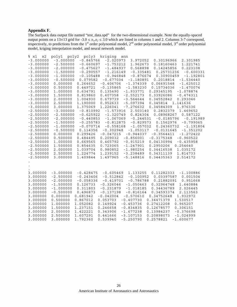
Appendix G. The Surfpack command input file named “four_dim_commands.spk” for the four-dimensional example. # Read in data Load[name = four_dim_data, file = 'four_dim_data_input.spd', n_predictors = 4, n_responses = 1] # Create a test set with evenly spaced points on an 11x11x11x1 grid CreateAxes[name = ax_4d, bounds = '0.5 1.5 | 1.5 4.5 | 0.7 1.0 | 0.7 '] CreateSample[name = test_data, axes = ax_4d, grid_points = (11,11,11,1), labels = (x1,x2,x3,x4)] CreateSurface[name=poly1_4d, data = four_dim_data, type = polynomial, order = 1] CreateSurface[name=poly2_4d, data = four_dim_data, type = polynomial, order = 2] CreateSurface[name=poly3_4d, data = four_dim_data, type = polynomial, order = 3] CreateSurface[name = kriging_4d, data = four_dim_data, type = kriging] CreateSurface[name = ann_4d, data = four_dim_data, type = ann] Evaluate[surface = poly1_4d, data = test_data, label = poly1] Evaluate[surface = poly2_4d, data = test_data, label = poly2] Evaluate[surface = poly3_4d, data = test_data, label = poly3] Evaluate[surface = kriging_4d, data = test_data, label = kriging] Evaluate[surface = ann_4d, data = test_data, label = ann] Save[data = test_data, file = 'test_data.spd'] Fitness[surface = poly1_4d, metric = rsquared] Fitness[surface = poly2_4d, metric = rsquared] Fitness[surface = poly3_4d, metric = rsquared] Fitness[surface = poly1_4d, metric = root_mean_squared] Fitness[surface = poly2_4d, metric = root_mean_squared] Fitness[surface = poly3_4d, metric = root_mean_squared] Fitness[surface = kriging_4d, metric = root_mean_squared] Fitness[surface = ann_4d, metric = root_mean_squared] Fitness[surface = poly1_4d, metric = press] Fitness[surface = poly2_4d, metric = press] Fitness[surface = poly3_4d, metric = press] Fitness[surface = kriging_4d, metric = press] Fitness[surface = ann_4d, metric = press]


27

Appendix H. The Surfpack data input file named “four_dim_data_input.spd” for the four-dimensional example. % x1 x2 x3 x4 f(x) 1.2 1.5 0.7 0.7 12.9 0.5 4.5 1 1 15.4 0.5 3 0.85 0.85 9.9 0.85 1.5 0.85 0.85 15.5 0.85 3 0.85 0.85 8.3 0.5 1.5 1 1 21.5 0.5 4.5 1 0.7 15.4 0.85 3 0.7 0.85 7.4 1.2 4.5 1 0.7 9.1 0.85 3 1 0.85 9.3 1.2 1.5 0.7 1 12 1.2 4.5 0.7 1 9.3 1.2 1.5 1 0.7 8.7 0.5 1.5 1 0.7 8.2 0.5 1.5 0.7 1 24 0.85 3 0.85 0.7 6.3 0.85 4.5 0.85 0.85 9.2 1.2 1.5 1 1 7.2 0.5 4.5 0.7 0.7 15.4 1.2 4.5 0.7 0.7 8.3 1.2 3 0.85 0.85 8.6 0.85 3 0.85 1 9.5 0.5 4.5 0.7 1 15.5 1.2 4.5 1 1 8.7 0.5 1.5 0.7 0.7 24.8 1 3 0.8 0.8 8.8 0.9 2.85714286 0.97142857 0.7 8.311 0.95 3.5 0.95714286 0.7 10.721 0.85 2.71428571 0.88571429 0.7 8.04 1.3 2.5 0.84285714 0.7 7.836 1.15 2.57142857 0.92857143 0.7 7.356 0.8 3.28571429 0.87142857 0.7 8.422 1 2.64285714 0.8 0.7 7.646 1.25 3.42857143 0.85714286 0.7 8.012 1.4 3.35714286 0.98571429 0.7 9.004 1.35 3 0.82857143 0.7 9.21 1.2 2.92857143 1 0.7 8.285 1.5 3.21428571 0.9 0.7 8.497 1.45 2.78571429 0.94285714 0.7 8.597 1.05 3.14285714 0.81428571 0.7 8.548 1.1 3.07142857 0.91428571 0.7 7.719 0.717 3.028 0.816 0.7 8.292


28

Appendix I. A portion of the Surfpack data output file named “test_data.spd” for the four-dimensional example with values for x1-x4 in columns 1-4, respectively, and the kriging interpolation results listed in the right-most column. The x1-x4 values correspond to an 11µ11µ11µ1 grid, with x4 = 0.7. This facilitates data plotting for this example. % x1 x2 x3 x4 . . . kriging . . . 0.5 1.5 0.7 0.7 . . . 24.8 0.5 1.5 0.73 0.7 . . . 23.9757 0.5 1.5 0.76 0.7 . . . 22.7329 0.5 1.5 0.79 0.7 . . . 21.1281 0.5 1.5 0.82 0.7 . . . 19.2459 0.5 1.5 0.85 0.7 . . . 17.1912 0.5 1.5 0.88 0.7 . . . 15.0803 0.5 1.5 0.91 0.7 . . . 13.0293 0.5 1.5 0.94 0.7 . . . 11.1448 0.5 1.5 0.97 0.7 . . . 9.51425 0.5 1.5 1.0 0.7 . . . 8.2 0.5 1.8 0.7 0.7 . . . 23.3635 0.5 1.8 0.73 0.7 . . . 22.6665 0.5 1.8 0.76 0.7 . . . 21.6008 0.5 1.8 0.79 0.7 . . . 20.2145 0.5 1.8 0.82 0.7 . . . 18.5802 0.5 1.8 0.85 0.7 . . . 16.7892 0.5 1.8 0.88 0.7 . . . 14.9425 0.5 1.8 0.91 0.7 . . . 13.1419 0.5 1.8 0.94 0.7 . . . 11.481 0.5 1.8 0.97 0.7 . . . 10.0372 0.5 1.8 1.0 0.7 . . . 8.8662 . . . 1.5 4.5 0.7 0.7 . . . 10.3617 1.5 4.5 0.73 0.7 . . . 10.2437 1.5 4.5 0.76 0.7 . . . 10.1557 1.5 4.5 0.79 0.7 . . . 10.1034 1.5 4.5 0.82 0.7 . . . 10.0909 1.5 4.5 0.85 0.7 . . . 10.1201 1.5 4.5 0.88 0.7 . . . 10.19 1.5 4.5 0.91 0.7 . . . 10.2973 1.5 4.5 0.94 0.7 . . . 10.4361 1.5 4.5 0.97 0.7 . . . 10.5988 1.5 4.5 1.0 0.7 . . . 10.7765


29

the surfpack software library for surrogate modeling of sparse

Documents