the svi implied volatility model and its calibration - · pdf filekungliga tekniska hogskolan...
TRANSCRIPT

Kungliga Tekniska Hogskolan
Master Thesis
The SVI implied volatility modeland its calibration
Author:
Alexander Aurell

KUNGLIGA TEKNISKA HOGSKOLAN
Abstract
Division of Mathematical Statistics
School of Engineering Sciences
Master of Science
The SVI implied volatility model
and its calibration
by Alexander Aurell
The SVI implied volatility model is a parametric model for stochastic implied volatil-
ity. The SVI is interesting because of the possibility to state explicit conditions on its
parameters so that the model does not generate prices where static arbitrage opportu-
nities can occur. Calibration of the SVI model to real market data requires non-linear
optimization algorithms and can be quite time consuming. In recent years, methods to
calibrate the SVI model that use its inherent structure to reduce the dimensions of the
optimization problem have been invented in order to speed up the calibration.
The first aim of this thesis is to justify the use of the model and the no static arbitrage
conditions from a theoretic point of view. Important theorems by Kellerer and Lee and
their proofs are discussed in detail and the conditions are carefully derived. The sec-
ond aim is to implement the model so that it can be calibrated to real market implied
volatility data. A calibration method is presented and the outcome of two numerical
experiments validate it.
The performance of the calibration method introduced in this thesis is measured in how
big a fraction of the total market volume the method manages to fit within the market
spread. Tests show that the model manages to fit most of the market volume inside the
spread, even for options with short time to maturity.
Further tests show that the model is capable to recalibrate an SVI parameter set that
allows for static arbitrage opportunities into an SVI parameter set that does not.
Key words: SVI, stochastic implied volatility, static arbitrage, parameter calibration,
Kellerer’s theorem, Lee’s moment formula.

Acknowledgements
I would like to thank my supervisours at ORC, Jonas Hagg and Pierre Backlund, for
introducing me to the topic. Throughout the project you have actively discussed my
progress and results and you have often inspired me to come up with new ideas and
approaches. Your constant support has been invaluable to me.
I would like to thank my advisor at KTH, Professor Boualem Djehiche, for great feed-
back, academic guidance and patience.
Thank you, Ty Lewis at ORC, for your many valuable inputs about the world of finance
and thank you, Tove Odland at KTH, for sharing your research and opinions on the
Nelder-Mead method with me.
Furthermore I would like to thank Fredrik Lannsjo and Helena E. Menzing for proof-
reading my thesis and commenting on the content.
Finally, I am most grateful for the support from Helena and my family during my entire
studies.
Alexander Aurell
Stockholm, September 2014
ii

Contents
Abstract i
Acknowledgements ii
Contents iii
List of Figures v
1 Introduction 1
1.1 Background . . . . . . . . . . . . . . . . . . . . . . . . . . . . . . . . . . . 1
1.2 Purpose of the thesis . . . . . . . . . . . . . . . . . . . . . . . . . . . . . . 2
1.3 Outline of the thesis . . . . . . . . . . . . . . . . . . . . . . . . . . . . . . 2
1.4 Delimitations . . . . . . . . . . . . . . . . . . . . . . . . . . . . . . . . . . 3
2 Kellerer’s Theorem and Lee’s Moment Formula 4
2.1 Stochastic implied volatility . . . . . . . . . . . . . . . . . . . . . . . . . . 5
2.2 Static arbitrage . . . . . . . . . . . . . . . . . . . . . . . . . . . . . . . . . 7
2.3 Kellerer’s theorem: derivation . . . . . . . . . . . . . . . . . . . . . . . . . 11
2.4 Kellerer’s theorem: implications on implied volatility . . . . . . . . . . . . 23
2.5 Asymptotic bounds on the implied volatility smile . . . . . . . . . . . . . 30
3 Parameterization of the implied volatility 36
3.1 Popular stochastic volatility models . . . . . . . . . . . . . . . . . . . . . 37
3.2 SVI parametrizations and their interpretation . . . . . . . . . . . . . . . . 40
3.3 The restriction: SSVI . . . . . . . . . . . . . . . . . . . . . . . . . . . . . 43
4 Parameter calibration 47
4.1 More parameter bounds . . . . . . . . . . . . . . . . . . . . . . . . . . . . 47
4.2 A new parameterization . . . . . . . . . . . . . . . . . . . . . . . . . . . . 49
4.3 Optimization . . . . . . . . . . . . . . . . . . . . . . . . . . . . . . . . . . 50
5 Numerical experiments 53
5.1 The Vogt smile: the elimination of static arbitrage . . . . . . . . . . . . . 53
5.2 Calibration to market data: the weighting of options . . . . . . . . . . . . 56
5.2.1 Data preperation . . . . . . . . . . . . . . . . . . . . . . . . . . . . 56
5.2.2 SPX options . . . . . . . . . . . . . . . . . . . . . . . . . . . . . . 57
iii

Contents iv
A Nelder-Mead method 69
B Spanning a payoff with bonds and options 73
C Call price derivative 75

List of Figures
2.1 S&P 500 (left vertical axis) and VIX (right vertical axis) monthly indexvalues plotted from January 1990 until today. Some important monthsare highlighted to visualize the negative correlation between the under-lying’s price process and the underlying’s volatility. Data gathered fromfinance.yahoo.com on 7/8/2014. . . . . . . . . . . . . . . . . . . . . . . . . 8
2.2 An example of a process that is not a martingale but for which thereexists a martingale with the same distribution at each discrete step. . . . 10
2.3 A process that is a martingale and has the same distribution at eachdiscrete step as the process in Figure 2.2. . . . . . . . . . . . . . . . . . . 10
3.1 The daily log returns of S&P 500 from January 3rd 1950 until today. Aslight clustering is visible. Data from finance.yahoo.com/ on 7/14/2014. . 39
5.1 Left plot: The implied volatility corresponding to the parameters in Equa-tion (5.1) is plotted against moneyness. Right plot: Durrleman’s condi-tion corresponding to the parameters in Equation (5.1) is plotted againstmoneyness. . . . . . . . . . . . . . . . . . . . . . . . . . . . . . . . . . . . 53
5.2 Solid lines correspond to the parameter set in Equation (5.3) and dashedlines correspond to the parameter set in Equation (5.1). Left plot: Impliedvolatility corresponding to the parameter sets is plotted against money-ness. Right plot: Durrleman’s condition corresponding to the parametersets is plotted against moneyness. . . . . . . . . . . . . . . . . . . . . . . . 54
5.3 The solid lines correspond to the, according to Equation (4.9), optimal setof JW parameters, the dashed red lines that lie on top of the solid linescorrespond to the original parameter set in Equation (5.1) and the deviantgreen dashed lines correspond to the parameter set in Equation (5.3). Leftplot: Implied volatility corresponding to the parameter sets is plottedagainst moneyness. Right plot: Durrleman’s condition corresponding tothe parameter sets is plotted against moneyness. . . . . . . . . . . . . . . 55
5.4 Market data from liquid, out-of-the-money options written on the SPXwith underlying price $1857.6. Upper plot: Prices for call options plottedagainst strike prices. The ask, mid and bid prices are not distinguishableon this scale. Lower plot: Implied volatilities for the same option thatwas treated in the upper plot plotted against moneyness. Here we candistinguish between the bid implied volatility, which are plotted as reddots, mid implied volatility, black dots, and ask implied volatility, bluedots. . . . . . . . . . . . . . . . . . . . . . . . . . . . . . . . . . . . . . . . 57
v

List of Figures vi
5.5 Implied volatility plotted against moneyness for four different times tomaturity. The red dots are bid implied volatility, the blue line is the SVIfit to mid implied volatility and the black dots are ask implied volatility.Only every third ask and bid implied volatility is plotted. . . . . . . . . . 58
5.6 The fraction of the total trading volume that the SVI implied volatil-ity manages to fit within the bid-ask call market price spread is plottedagainst time to maturity for the implied volatility smile that has beenfitted. . . . . . . . . . . . . . . . . . . . . . . . . . . . . . . . . . . . . . . 59
5.7 The concentration of trading volume around the origin. Left axis: Therelative trading volume, blue dots, is plotted against moneyness. Rightaxis: The accumulated relative trading volume, red line, is plotted againstmoneyness. . . . . . . . . . . . . . . . . . . . . . . . . . . . . . . . . . . . 60
5.8 Two possible choices of option weights. Left axis: The relative tradingvolume is plotted against moneyness. Most of the volume is traded be-tween −0.1 and 0.05, but some outliers can be seen on the negative part ofthe x-axis. Right axis: The vega of the option is plotted against money-ness. The sensitivity of the option price to changes in volatility is greatestaround the origin and decays quickly in both directions. . . . . . . . . . . 61
5.9 The fraction of the market which was fitted inside the call spread as afunction of the number of options used in the calibration. . . . . . . . . . 62
5.10 New SVI implied volatility fit using weights and caps in the calibration.The red dots are bid implied volatility, the blue line is the SVI fit to midimplied volatility and the black dots are ask implied volatility. Only everythird ask and bid implied volatility is plotted. . . . . . . . . . . . . . . . . 64
5.11 The fraction of the total trading volume that the new SVI implied volatil-ity, calibrated with weights and caps, manages to fit within the bid-ask callprice spread is plotted against time to maturity for the implied volatilitysmile that has been fitted. . . . . . . . . . . . . . . . . . . . . . . . . . . . 65
5.12 The amount that the SVI generated call prices miss the bid-ask call pricespread at each strike plotted for the four times to maturity. . . . . . . . . 65
5.13 Durrleman’s condition plotted corresponding to the new SVI impliedvolatility for the four times to maturity. . . . . . . . . . . . . . . . . . . . 66
A.1 One iteration of the Nelder-Mead algorithm with ρ = 1, η = 2, c = 1/2and σ = 1/3. . . . . . . . . . . . . . . . . . . . . . . . . . . . . . . . . . . 72

Chapter 1
Introduction
This introduction will briefly state the background, purpose and delimitations of the
work done in this thesis. Also a summary of all the chapters is given.
1.1 Background
When pricing financial contracts such as options it is common practice to use the Black-
Scholes framework. Black-Scholes assumes that options with all parameters equal, except
the strike price, are to be priced with the same implied volatility parameter value. This
however stands in contradiction with the real world where market prices imply that the
volatility depends on the strike price. One way that practioners handle this problem is
to create implied volatility surfaces. An implied volatility surface is a function,
(Time to maturity, Strike) 7→ Implied volatility(Time to maturity, Strike).
The work flow is basically as follows:
(1) Provided by option prices from the market for a range of strikes and maturities
one gets the corresponding implied volatilities by inverting the Black-Scholes price
function.
(2) Use the result from (1) to create an implied volatility surface for all (Strike,Maturity)-
points.
(3) When pricing an option with a given strike and maturity get the implied volatility
to use from the surface.
1

Chapter 1. Introduction 2
There are several popular models that are used for the surface construction in (2). The
stochastic volatility inspired, or SVI, model of the implied volatility surface was originally
created at Merrill Lynch in 1999 and was introduced to the public in the presentation [1].
The model has two key properties that are often stated in the literature that followed [1]
as reasons for its popularity amongst practitioners. It satisfies Lee’s Moment Formula,
a model free result that specifies the asymptotics for implied volatility. Therefore, the
SVI model is valid for extrapolation far outside the avaliable data. Furthermore, it is
stated that the SVI model is relatively easy to calibrate to market data so that the
corresponding implied volatility surface is free of calendar spread arbitrage. The recent
development of the SVI model has been towards conditions guaranteing the abscence
of butterfly arbitrage. In [2] this problem is solved by restricting the parameters in the
SVI model.
1.2 Purpose of the thesis
The purpose of this thesis is to motivate the usage of the SVI model from a theoretical
point of view, and implement the SVI model so that a parametrized implied volatility
surface can be fitted to market data. Furthermore, the model should be able to detect
static arbitrage and eliminate it by a recalibration. The thesis aims to give thorough
explanations of the underlying theoretical results, and do a complete derivation of the
no static arbitrage conditions. It also aims to in detail present a calibration method for
the SVI parameters to real market implied volatility data and evaluate its accuracy.
1.3 Outline of the thesis
This thesis is divided into five chapters. Chapter 1 introduces the topic of this thesis,
states the purpose of it, summarizes it and states the delimitations that were done.
In Chapter 2, two underlying theoretical results are presented. Conditions on the call
prices that guarantees absence of static arbitrage is derived using Kellerer’s theorem and
these conditions are translated into conditions on the implied volatility surface. Lee’s
Moment Formula is recalled and its implications are discussed. In Chapter 3, the SVI
parameterization for implied volatility and variations of it are presented. A concrete
method for eliminating static arbitrage in the implied volatility smile is constructed. In
Chapter 4, the calibration method used to fit the SVI model to market data is described
in detail. The final chapter, Chapter 5, numerical results of the calibration method are
presented.

Chapter 1. Introduction 3
1.4 Delimitations
Some proofs are omitted and the reason for this is either their extensive length or that
they are unrelevant to the surrounding context. If a proof is omitted, a reference is given
to a complete proof.
Calendar spread arbitrage is only treated in theory. Sufficient conditions for the elim-
ination of calendar spread arbitrage are derived together with the sufficient conditions
for elimination of butterfly arbitrage, but no numerical experiments are done trying to
eliminate calendar spread arbitrage from SVI surfaces fitted to real market data.
Numerous delimitations are made in the last chapter, mainly because of the lack of time.
The speed of the calibration is not investigated. Only one set of weights are used in the
optimization and only one type of options, call and put options on the S&P 500, are
used.
The error of the fit is quantified in two ways, the fraction of the total market that the
SVI fitted inside the price spread and the distance from the SVI fitted prices to the price
spread. These results are not compared to the results of other calibration methods.

Chapter 2
Kellerer’s Theorem and Lee’s
Moment Formula
In this chapter, a theoretical approach to the elimination of static arbitrage in an implied
volatility surface will be presented. It begins with setting up the model framework used
in the rest of the thesis and then gives a short introduction to stochastic implied volatility.
After that, sufficient conditions for the absence of static arbitrage on the surface of call
prices,
(Time to maturity, Strike) 7→ Call price(Time to maturity, Strike),
are derived through an application of Kellerer’s Theorem. At every time to maturity
the density of the underlying’s price process martingale is matched with the density of
a martingale that has the Markov property. The conditions on the call surface are then
translated into conditions for the implied volatility surface.
Additionally, Lee’s Moment Formula is examined. It is a model free result that states
conditions on the asymptotes of implied volatility smiles. Iimplied volatility smile is the
name in finance for a time to maturity-section of the implied volatility surface. For a
fixed, positive t,
Implied volatility smile(Strike) = Implied volatility(Time to maturity = t,Strike)
All models that extrapolate implied volatility generated from market data in the strike
direction should satisfy Lee’s Moment Formula.
4

Chapter 2. Kellerer’s Theorem and Lee’s Moment Formula 5
2.1 Stochastic implied volatility
The model is set up in a probability space (Ω, (Ft, t ≥ 0),Q). The filtration (Ft, t ≥ 0),
indexed by the time t, is generated by a 2-dimensional Brownian motion (B0, B1) and
Q is the measure under which the underlying’s discounted price process is a martin-
gale. There are M + 2 traded objects in the model, the underlying with price process
S(t) = St, a set of M European call options with strike prices and times to maturity
(K,T ) written on St and a risk-free investment with constant, positive interest rate r.
The underlying price process is assumed to be represented by the dynamics
dSt = rStdt+ σStdB0t , (2.1)
where σ is stochastic. The Black-Scholes price of a call option is given by the Black-
Scholes formula stated in Equation (2.2) and the implied volatility. The implied volatility
will be denoted by σimp. The name and notation emphesizes that it is implied from the
Black-Scholes pricing formula. Hence, there is a difference between the volatility of the
underlying’s price process, σ from Equation (2.1), and the implied volatility, σimp from
Equation (2.2). The model is not set up in a Black-Scholes world since σ is not assumed
to be constant but depends on both strike price and time to maturity. Therefore, the
Black-Scholes formula merely serves as a convenient tool to describe option prices. Note
that σimp does not necessarily equal σ. An important note to bear in mind as motivation
for using implied volatility, is that it is generally easier to observe the implied volatility
on the market than it is to observe the volatility of the underlying’s price process.
The formal definition of implied volatility of an option is the parameter σimp that gives
the observed option price, C, when inserted into the Black-Scholes call price formula,
CBS(τ,K, τσ2imp;S, r, t) = StN (d1)− e−rτKN (d2). (2.2)
Here N (x) is the cumulative distribution function of a standard normally distributed
random variable, t is the current time, T is the maturity time for the option, τ = T − tis the time to maturity for the option and d1 and d2 are the Black-Scholes auxiliary
functions,
d1(τ,K, τσ2imp;S, r, t) =
log (St/K) + τr + τσ2imp/2√
τσ2imp
, (2.3)
d2(τ,K, τσ2imp;S, r, t) =
log (St/K) + τr − τσ2imp/2√
τσ2imp
.

Chapter 2. Kellerer’s Theorem and Lee’s Moment Formula 6
The dependece on the variables S, r, and T is denoted behind a semicolon, separating
them from τ,K and σ. This is done to clarify that in this thesis, they are of lesser
interest than the variables τ,K and σimp. More than often, the dependence of the
variables behind the semicolon will be surpressed. This paragraph is summarized in the
following definition.
Definition 1. (Implied volatility) Let a call option be written on the underlying S at
time t with strike price K and expiry time T . Let the observed market price for this
option be C. The implied volatility of the option is the unique value of σimp that solves
C = CBS(τ,K, τσ2imp;S, r, t).
An alternative, but equivalent, definition of implied volatility can be stated by replacing
the underlying’s price process with the forward price.
Definition 2. The forward price process of the underlying S is
F (t, τ) = F[t,t+τ ] = erτSt.
If using F[t,t+τ ] instead of St, the implied volatility of an option is the parameter σimp
that gives the observed compounded option price, Cerτ , when substituted into what is
called the Black call price formula,
CB(τ,K, τσ2imp;F, r, t) = F[t,t+τ ]N (d1)−KN (d2). (2.4)
By using the forward price instead of the underlying’s price process, the auxiliary func-
tions in Equation (2.3) simplify to
d1(τ,K, τσ2imp;F, r, t) =
log(F[t,t+τ ]/K
)+ 1
2σ2impτ√
τσ2imp
, (2.5)
d2(τ,K, τσ2imp;F, r, t) =
log(F[t,t+τ ]/K
)− 1
2σ2impτ√
τσ2imp
.
The Black call price formuka will be used instead of the Black-Scholes call price formula
especially in Appendix C.
So far, all we have said about σ is that it is random. If this is the case, σimp should also
be random. This is in accordance with observations of the real market, where volatility
across strike and across time is not constant but behaves in a stochastic manner. Hence
let the implied variance, σ2imp, for an option written on S with maturity T and strike K

Chapter 2. Kellerer’s Theorem and Lee’s Moment Formula 7
have the following dynamics,
dσ2imp(τ,K, τσ2
imp;S, r, t) = α(τ,K, τσ2imp;S, r, t) dt+ ηβ(τ,K, τσ2
imp;S, r, t) dB1t , (2.6)
where 〈dB0t , dB
1t 〉 = ρdt, ρ ∈ [−1, 1]. In Chapter 8.6 in [3], it is derived that the
Black-Scholes model with non-constant but deterministic implied volatility is retrieved
in the limit η → 0. This is not necessarily an advantage for the model performance,
however it is almost a practical requirement as the Black-Scholes model is the core of
the intuition of practitioners. The choice of specifying the dynamics of the implied vari-
ance instead of the implied volatility is made to follow the line of literature in [3] and [4].
Being able to model correlation between the underlying’s price process and the cor-
responding implied volatility is necessary, as it can be observed on the real market. In
Figure 2.1, historical data for the S&P 500 index and the VIX index are presented. The
S&P 500 is a stock market index based on the performance of the 500 largest companies
which are listed at the New York Stock Exchange or the NASDAQ, while the VIX index
is a measure of the implied volatility of the S&P 500 index. In this figure it can be seen
that when the S&P 500 suffers a severe drop, such as during the Russian crisis of 1998,
the end of the IT-bubble in 2002, the U.S. housing bubble in 2008 and the European
sovereign debt crisis in 2011, the VIX index rose dramatically. Heuristically, a negative
correlation between the S&P 500 and the VIX can be established.
2.2 Static arbitrage
This section introduces the concept of static arbitrage and how it differs from dynamic
arbitrage, the kind of arbitrage that is treated in The Fundamental Theorem of Asset
Pricing.
Definition 3 (Dynamic arbitrage opportunity). A dynamic arbitrage opportunity is a
costless trading strategy that gives a positive future profit with positive probability and
has no probability of a loss.
The problem with this definition is that the opportunity depends on a too big set of
data than is desired or even available in practical situations. For example, in continuous
time the definition depends on the path properties of underlying’s price processes. In
practice only past prices at discrete times are observable. Working with static arbitrage,
which is defined in Definition 4 below, suits this situation.

Chapter 2. Kellerer’s Theorem and Lee’s Moment Formula 8
0 50 100 150 200 250 3000
1000
2000S&P 500 and VIX monthly index levels from 2nd January 1990 until today
Months after 2nd January 1990
S&
P50
0 in
dex
leve
l
0 50 100 150 200 250 3000
50
100
VIX
inde
x le
vel
August 1998
September2002
October2008
September2011
Figure 2.1: S&P 500 (left vertical axis) and VIX (right vertical axis) monthly indexvalues plotted from January 1990 until today. Some important months are highlightedto visualize the negative correlation between the underlying’s price process and the
underlying’s volatility. Data gathered from finance.yahoo.com on 7/8/2014.
Definition 4 (Static arbitrage opportunity). A static arbitrage opportunity is a dy-
namic arbitrage opportunity where positions in the underlying at a particular time only
can depend on time and actual corresponding price.
The Fundamental Theorem of Asset Pricing tells us that no dynamic arbitrage is equiv-
alent to the existence of an equivalent martingale measure. From Definition 4, the
following relaxed connection for static arbitrage was established in [5] and [6]. Instead
of starting with a complete probability space and seeking martingales via a change of
measure, as is the case in the elimination of dynamic arbitrage, the authors of [5] and
[6] start with a family of densities, q(X, t), t > 0, of random variables, Xt, t > 0,indexed by t. These densities can be interpreted as measures, which will be done in
Section 2.3. The authors proceed to show that if there exist some probability space on
which it is possible to define a martingale M(t) with the Markov property so that the
law of M(t) is q(M, t) for each t, then the process X = (Xt, t > 0) does not admit static
arbitrage. We will refer to these laws, or densities, as t-marginals and we will call two
proceeses that agree on their t-marginals for all t associated processes.

Chapter 2. Kellerer’s Theorem and Lee’s Moment Formula 9
Definition 5 (Associated process). If (Xt; t ≥ 0) and (Yt; t ≥ 0) are two stochastic
processes indexed by t, they are said to be associated if they have the same t-marginals
for all t.
The theory that tell us whether an underlying asset, observable through call option
prices on the market, and a process that is a martingale are associated or not is based
on a theorem by Kellerer [7], which will be recalled in Section 2.3. The Markov property
for stochastic processes is defined in Definition 6, which is the definition of Durrett [8].
Definition 6 (Markov property for stochastic processes). Let (Ω,F ,P) be a probability
space with a filtration (Fs, s > 0) and let (S,S) be a measurable space. An Fs-adapted
process X = (Xt, t > 0) : Ω 7→ S is said to have the Markov property if for each s ∈ Sand each s, t > 0 with s < t,
P (Xt ∈ s|Fs) = P (Xt ∈ s|Xs) .
Equivalently, the process has the Markov property if for all t ≥ s ≥ 0 and for all bounded
and measurable f : S 7→ R,
E [f(Xt)|Fs] = E [f(Xt)|Xs] .
An easy application of the tower property of conditional expectations shows that no
dynamic arbitrage implies no static arbitrage, since the information set available when
trading under no static arbitrage is a subset of that used when trading under no dynamic
arbitrage. On the other hand, no static arbitrage does not imply no dynamic arbitrage,
and this is best illustrated through a reproduction of an example in [6]. Let a process
be defined on a grid with two levels, as in Figure 2.2. Call the process on the grid in
Figure 2.2 for Mt. The procees Mt can not be a martingale since E[M1|M0.5] 6= M0.5.
But on the other hand, Mt has exactly the same t-marginals as the process in Figure 2.3
that goes up or down one price tick at each node with equal probability, and this process
is a martingale!

Chapter 2. Kellerer’s Theorem and Lee’s Moment Formula 10
0 0.5 1
80
90
100
110
120
A two level process and its transition probabilities
Time
Pric
e
90
110
80
100
120
1/2
1/2
1/4
1/4
3/4
1/4
1/2
Figure 2.2: An example of a process that is not a martingale but for which thereexists a martingale with the same distribution at each discrete step.
0 0.5 1
80
90
100
110
120
A two level process that is a martingale and its transition probabilities
Time
Pric
e
90
80
100
1/2
120
1/2
1/2
1/2
1/2
1101/2
Figure 2.3: A process that is a martingale and has the same distribution at eachdiscrete step as the process in Figure 2.2.

Chapter 2. Kellerer’s Theorem and Lee’s Moment Formula 11
2.3 Kellerer’s theorem: derivation
In this section, conditions for no static arbitrage on a call surface for European options
are derived using Kellerer’s theorem, which will be proved following the work of Hirsch,
Roynette and Yor in [9] and [10]. We begin with some definitions.
Definition 7 ( Mf ). Mf is the set of all probability measures µ on R such that∫|x|µ(dx) <∞.
Definition 8 ( Call function ). For µ ∈Mf and x ∈ R, the corresponding call function
is defined as
Cµ(x) =
∫R
(y − x)+µ(dy).
From these definitions, we can derive three properties of the call function Cµ.
Proposition 1. Cµ is non-negative and convex.
Proof. Since (y−x)+ ≥ 0 for all (x, y) ∈ R2 and µ ∈Mf , Cµ is non-negative. Convexity
follows from the non-negativity of µ together with the following calculation,
∂2Cµ∂x2
(x) =∂
∂x
(∂
∂x
∫R
(y − x)+µ(dy)
)=
∂
∂x
∫ ∞x−µ(dy)
= µ(x).
Proposition 2. Cµ satisfies
limx→∞
Cµ = 0.
Proof. Let fn = (y−n)+ for n ∈ Z, and let gn = f0−fn. Then gn is an increasing, non-
negative sequence of measurable functions that converges pointwise to f0 and monotone
convergence applies to gn,
limn→∞
∫Rgn(y)µ(dy) =
∫R
limn→∞
gn(y)µ(dy).
Thus we have
limn→∞
(∫Rf0(y)µ(dy)−
∫Rfn(y)µ(dy)
)=
∫Rf0(y)µ(dy)−
∫R
limn→∞
fn(y)µ(dy)
=
∫Rf0(y)µ(dy),

Chapter 2. Kellerer’s Theorem and Lee’s Moment Formula 12
and
limx→∞
Cµ(x) = limn→∞
∫Rfn(y)µ(dy)
= 0.
Proposition 3. There exists a real number a so that
limx→−∞
Cµ(x) + x = a.
Proof. Note first that (y − x)+ = supy, x − x. Hence, since µ ∈Mf ,
Cµ(x) =
∫R
(y − x)+µ(dy)
=
∫R
supy, xµ(dy)− x∫Rµ(dy)
=
∫R
supy, xµ(dy)− x,
so we get
limx→−∞
Cµ(x) + x = limx→−∞
∫R
supy, xµ(dy).
Now let fn(y) = supy,−n for n ∈ Z, and let gn(y) = f0(y) − fn(y). Then gn is an
increasing, non-negative sequence of measurable functions that converges pointwise to
f0 − y and monotone convergence applies,
limn→∞
∫Rgn(y)µ(dy) =
∫R
limn→∞
gn(y)µ(dy).
Thus, we get
limn→∞
(∫Rf0(y)µ(dy)−
∫Rfn(y)µ(dy)
)=
∫Rf0(y)µ(dy)−
∫R
limn→∞
fn(y)µ(dy)
=
∫Rf0(y)µ(dy)−
∫Ryµ(dy),
and the reuslt follows,
limx→−∞
Cµ(x) + x = limn→∞
∫Rfn(y)µ(dy) (2.7)
=
∫Ryµ(dy) <∞.

Chapter 2. Kellerer’s Theorem and Lee’s Moment Formula 13
These three properties can also serve as a characterization of a probability measure, as
the next proposition will tell us. This is a useful direction for our purpose.
Proposition 4. If C : R 7→ R has the properties in Proposition 1, Proposition 2 and
Proposition 3,
P1. C is non-negative and convex,
P2. C(x)→ 0 as x→∞,
P3. There exists a real number a such that C(x) + x→ a as x→ −∞,
then there exists a unique µ ∈Mf such that C = Cµ. Furthermore, this µ is the second
derivative of C in the sense of distributions.
Proof. The proof of this direction can be found either in Proposition 2.1 of [10] or Lemma
7.23 of [11]. A slightly different version of the theorem is proven in Theorem 2.1 of [12].
The proof is omited here.
Additionally, three useful properties of the call function can be derived.
Proposition 5. If µ ∈Mf then
i) for all x1 ∈ R and x2 ∈ R such that x1 ≤ x2,
0 ≤ Cµ(x1)− Cµ(x2) ≤ x2 − x1,
ii) for all x ∈ RCµ(x) + x−
∫Rxµ(dy) =
∫R
(x− y)+µ(dy),
iii) limx→−∞
Cµ(x) + x =
∫Ryµ(dy).
Proof of i). Using the rewriting of the integrand in the call function from the proof of
Proposition 3,
(y − x)+ = supx, y − x,
the upper inequality can be derived,
Cµ(x1)− Cµ(x2) =
∫R
supy, x1µ(dy)− x1 −∫R
supy, x2µ(dy) + x2
= x2 − x1 +
∫R
supy, x1 − supy, x2µ(dy)︸ ︷︷ ︸≤0
≤ x2 − x1.
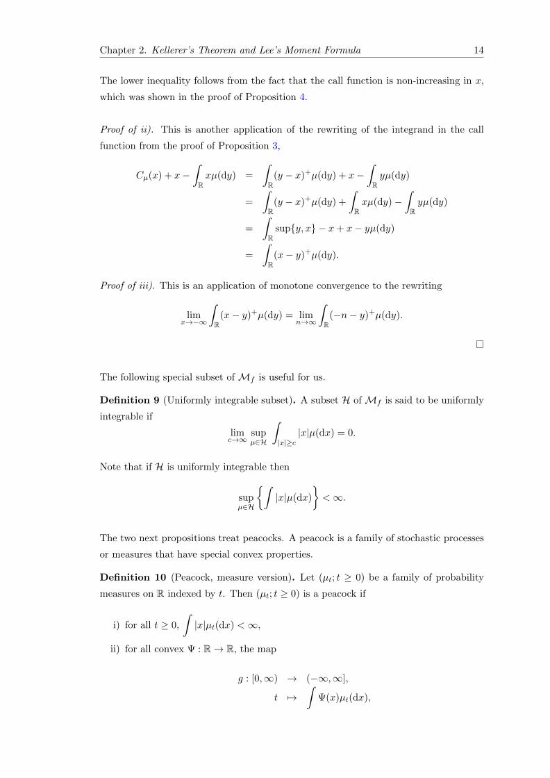
Chapter 2. Kellerer’s Theorem and Lee’s Moment Formula 14
The lower inequality follows from the fact that the call function is non-increasing in x,
which was shown in the proof of Proposition 4.
Proof of ii). This is another application of the rewriting of the integrand in the call
function from the proof of Proposition 3,
Cµ(x) + x−∫Rxµ(dy) =
∫R
(y − x)+µ(dy) + x−∫Ryµ(dy)
=
∫R
(y − x)+µ(dy) +
∫Rxµ(dy)−
∫Ryµ(dy)
=
∫R
supy, x − x+ x− yµ(dy)
=
∫R
(x− y)+µ(dy).
Proof of iii). This is an application of monotone convergence to the rewriting
limx→−∞
∫R
(x− y)+µ(dy) = limn→∞
∫R
(−n− y)+µ(dy).
The following special subset of Mf is useful for us.
Definition 9 (Uniformly integrable subset). A subset H ofMf is said to be uniformly
integrable if
limc→∞
supµ∈H
∫|x|≥c
|x|µ(dx) = 0.
Note that if H is uniformly integrable then
supµ∈H
∫|x|µ(dx)
<∞.
The two next propositions treat peacocks. A peacock is a family of stochastic processes
or measures that have special convex properties.
Definition 10 (Peacock, measure version). Let (µt; t ≥ 0) be a family of probability
measures on R indexed by t. Then (µt; t ≥ 0) is a peacock if
i) for all t ≥ 0,
∫|x|µt(dx) <∞,
ii) for all convex Ψ : R→ R, the map
g : [0,∞) → (−∞,∞],
t 7→∫
Ψ(x)µt(dx),

Chapter 2. Kellerer’s Theorem and Lee’s Moment Formula 15
is increasing.
Proposition 6. Let the family of measures (µt; t ≥ 0) be in Mf . Let furthermore∫R xµt(dy) be independent of t. Then (µt; t ≥ 0) is a peacock if and only if for all x ∈ R,
the map t 7→ C(t, x), where C(t, x) = Cµt(x), is increasing.
Proof. The assumption that (µt; t ≥ 0) is in Mf makes the family of measures satisfy
condition i) of Definition 10. Thus let us focus on condition ii) of Definition 10.
Assume that (µt; t ≥ 0) is a peacock, and hence satisfies condition ii) of Definition 10.
Let Ψ(x) = (x − c)+, c ∈ R. Then C(t, x) =∫
Ψ(x)µt(dx), and the map t → C(t, x) is
increasing. The proof of the other direction is long. It can be derived from Corollary
2.62 together with Theorem 2.58 in [11] and it is omitted here.
Proposition 7. Assume that (µt; t ≥ 0) is a peacock. Assume furthermore that∫R xµt(dy) is independent of t. Then
1. the set µt; 0 ≤ t ≤ T is uniformly integrable,
2. lim|x|→∞
sup C(t, x)− C(s, x) : 0 ≤ s ≤ t ≤ T = 0.
Proof of 1. Note that if c ≥ 0,
|y|I|y|≥c ≤ (2|y| − c)+ .
Then, since (2|y| − c)+ is convex and (µt; t ≥ 0) is a peacock,
supt∈[0,T ]
∫|y|≥c|y|µt(dy) ≤
∫R
(2|y| − c)+ µT (dy).
Let fn(y) = (2|y| − n)+ for n ∈ N, then fn is a sequence of measurable functions with
the pointwise limit 0. Also, |fn(y)| = fn(y) ≤ 2|y| for all n ∈ N, and under the law of
µT ,
2
∫R|y|µT (dy) <∞,
since µT ∈Mf . Hence by dominated convergence
limc→∞
supt∈[0,T ]
∫|y|≥c|y|µt(dy)
≤ lim
c→∞
∫R
(2|y| − c)+ µT (dy)
= limn→∞
∫Rfn(y)µT (dy) = 0,
which proves that µt; 0 ≤ t ≤ T is uniformly integrable.

Chapter 2. Kellerer’s Theorem and Lee’s Moment Formula 16
Proof of 2. Since (y − x)+ is a convex function in x and (µt; t ≥ 0) is a peacock,
condition ii) in Definition 10 tells us that the call function is an increasing function in
t and we get the inequality
supC(t, x)− C(s, x) : 0 ≤ s ≤ t ≤ T ≤ C(T, x)− C(0, x).
By Proposition 1, the call function is non-negative, so C(0, x) ≥ 0 and
supC(t, x)− C(s, x) : 0 ≤ s ≤ t ≤ T ≤ C(T, x).
By Proposition 2,
limx→∞
supC(t, x)− C(s, x) : 0 ≤ s ≤ t ≤ T = 0,
and we have proven the statement for large positive limit of x.. Now we have to prove
it in the large negative limit of x. Since∫R xµt(dy) is independent of t,
C(t, x)− C(s, x) =
(C(t, x) + x−
∫Rxµt(dy)
)−(C(s, x) + x−
∫Rxµs(dy)
).
By the same arguments as above, C(t, x) is increasing in t, so
supC(t, x)− C(s, x) : 0 ≤ s ≤ t ≤ T ≤ C(T, x) + x−∫RxµT (dy).
Taking the large negative limit and using Proposition 3 completes the proof,
limx→−∞
supC(t, x)−C(s, x) : 0 ≤ s ≤ t ≤ T ≤ limx→−∞
(C(T, x) + x−
∫RxµT (dy)
)= 0.
In the end of this section we will connect two processes via association, defined in
Definition 5. The connection will be made through an application of the following
uniqueness theorem for solutions of the Fokker-Planck equation.
Theorem 1 (M. Pierre’s Uniqueness Theorem for the Fokker-Planck Equation). Let
the map
a : R+ × R → R+
(t, x) 7→ a(t, x)
be continuous such that a(t, x) > 0 for all (t, x) ∈ (0,∞) × R, and let µ ∈ Mf . Then
there exists at most one family of probability measures (p(t,dx); t ≥ 0) such that

Chapter 2. Kellerer’s Theorem and Lee’s Moment Formula 17
(FP1) t 7→ p(t,dx) is weakly continuous,
(FP2) p(0, dx) = µ(dx) and
∂p
∂t− ∂2
∂x2(ap) = 0, in S′ ((0,∞)× R) ,
where S′ is the space of Schwartz distributions.
Proof. The proof is omitted for two reasons. Most importantly, it is not relevant to the
understanding of Kellerer’s theorem. Secondly, it is very long. A thorough version of
the proof can be found in [13], Chapter 6.1.
When the underlying’s price process and the martingale have been connected, we would
like to establish the Markov property for the martingale. A stronger property than the
Markov property will be established for a certain class of stochastic processes in the next
theorem, but first we need some new notation. As was done in [10], Definition 4.1 from
[14] is used; if (Xt; t ≥ 0) is an R-valued stochastic process then FX is the filtration
generated by X,
FXt = σXs, s ≤ t, ∀ t ≥ 0.
For a Lipschitz continuous function f : R → R, let L(f) denote its Lipschitz constant.
Let X be an R-valued process. We say X has the Lipschitz-Markov property if there
exists a Lipschitz continuous f : R→ R with Lipschitz constant L(f) < 1 such that for
all bounded and continuous functions g : R→ R with L(g) ≤ 1 and all s ∈ [0, t],
f(Xs) = E[g(Xt) | FXs
].
The Lipschitz-Markov property implies the Markov property defined in Definition 6.
The following theorem tells us that a certain kind of process has the Lipschitz-Markov
property.
Theorem 2. Let the map
σ : R+ × R → R,
(t, x) 7→ σ(t, x),
be continuous and such that ∂xσ exists and is continuous. Let furthermore X0 be an
integrable random variable and (Bt; t ≥ 0) be a standard Brownian motion independent
of X0. Then
Xt = X0 +
∫ t
0σ(s,Xs) dBs

Chapter 2. Kellerer’s Theorem and Lee’s Moment Formula 18
has a unique solution with the Lipschitz-Markov property.
Proof. The proof is omitted here for the same reason as the proof of Theorem 1. The
proof can be found in [10].
Finally we arrive to the theorem that establishes the connection.
Theorem 3 (Kellerer’s Theorem). Let (Xt; t ≥ 0) be an R-valued integrable stochastic
process indexed by t with t-marginals (p(t, x); t ≥ 0). Let furthermore∫R xp(t,dx) be
independent of t, and let
C : R+ × R → R+,
(t, x) 7→ E[(Xt − x)+
].
Asssume the following,
1. C ∈ C2,2(R+ × R) and
p(t, x) =∂2C
∂x2(t, x), ∀(t, x) ∈ R+ × R,
2. p is positive on R+ × R, ∂tC is positive on (0,∞)× R and
σ(t, x) =
√2
p
∂C
∂t, ∀(t, x) ∈ R+ × R.
Then
Zt = Z0 +
∫ t
0σ(s, Zs) dBs
has a unique strong solution (Yt; t ≥ 0) which is a martingale associated with (Xt; t ≥ 0)
satisfying the Lipschitz-Markov property. This in turn implied absence of static arbitrage
on the call surface C by the discussion in Chapter 2.2.
Proof. The proof will be divided into three steps. First, using Theorem 1, we prove that
X and Y are associated processes. In the second step we prove that Y is a martingale.
In the third step we show that Y has the Lipschitz-Markov property, using Theorem 2.
Step 1. We start with investigating the process X. Recall that the elements of the
family (p(t, x); t ≥ 0) are the t-marginals of (Xt; t ≥ 0). Let a(t, x) = σ2(t, x)/2, then
∂2
∂x2(ap) =
∂3
∂x2∂tC =
∂
∂tp.

Chapter 2. Kellerer’s Theorem and Lee’s Moment Formula 19
Also t 7→ p(t, x) is a continuous function since ∂xxC is continuous by assumption 1. in
the statement of the theorem. Hence (p(t, x); t ≥ 0) satisfies the Fokker-Planck equation.
Furthermore, since a(t, x) is positive everywhere, Theorem 1 tells us that (p(t, x); t ≥ 0)
is the unique family of measures that does this.
We now investigate the process Y . Let ϕ be a real-valued function on the real line
that is twice differentiable and has compact support within Y (R), the image of Y . Ito’s
fomula says,
dϕ(Yt) =∂ϕ
∂x(Yt) dYt +
1
2
∂2ϕ
∂x2(Yt) d〈Y 〉t.
The dynamics of Yt is by Ito’s formula,
dYt = 0 dt+ σ(t, Yt) dBt + 0 dt,
d〈Y 〉t = σ2(t, Yt) dt.
Hence, we get
dϕ(Yt) = σ(t, Yt)∂ϕ
∂x(Yt) dBt +
1
2σ2(t, Yt)
∂2ϕ
∂x2(Yt) dt.
Integrating from 0 to t, with a(t, x) = σ2(t, x)/2, yields,
ϕ(Yt)− ϕ(Y0) =
∫ t
0σ(s, Ys)
∂ϕ
∂x(Ys) dBs +
∫ t
0a(s, Ys)
∂2ϕ
∂x2(Ys) ds.
Under expectation conditioned on Y0 = y0, the first integral vanishes since ϕ ∈ C2(Y (R)).
With q(t, Y ) as the law of Yt, we get∫Yt(R)
ϕ(x)q(t,dx) + y0 =
∫Yt(R)
∫ t
0a(s, x)
∂2ϕ
∂x2(x)q(ds, dx).
The last step is to take the derivative with respect to time. In the proceeding calcu-
lations, the fact that ϕ(Yt) has compact support in the interior of Yt(R) is used in the
partial integration. The left hand side becomes,
∂
∂t
∫Yt(R)
ϕ(x)q(t,dx) + y =
∫Yt(R)
ϕ(x)∂q
∂t(t,dx),

Chapter 2. Kellerer’s Theorem and Lee’s Moment Formula 20
and the right hand side becomes,
∂
∂t
∫Yt(R)
∫ t
0a(s, x)
∂2ϕ
∂x2q(ds, dx) =
∫Yt(R)
a(t, x)∂2ϕ
∂x2q(t,dx)
=
[a(t, x)
∂ϕ
∂xq(t, x)
]∂Yt(R)
−∫Yt(R)
∂ϕ
∂x
∂
∂x(a(t, x)q(t,dx))
= −[ϕ(x)
∂
∂x(a(t, x)q(t, x))
]∂Yt(R)
+
∫Yt(R)
ϕ(x)∂2
∂x2(a(t, x)q(t,dx))
=
∫Yt(R)
ϕ(x)∂2
∂x2(a(t, x)q(t,dx)) .
To summarize, we have shown that∫Yt(R)
ϕ(x)∂q
∂t(t,dx) =
∫Yt(R)
ϕ(x)∂2
∂x2(a(t, x)q(t,dx)) ,
but this is nothing else than (FP2) in Theorem 1, in the sense of distributions. Thus
the law of the t-marginals of (Yt; t ≥ 0) satisfies the Fokker-Planck equation with the
same a(t, x) as the law of the t-marginals of (Xt; t ≥ 0). Therefore, by Theorem 1, the
laws are the same and by defintion, X and Y are associated.
Step 2. Note one thing about condition expectations: by standard definition, E[X | Y ] is
the unique random variable such that for all bounded and measurable random variables
Z,
E[E[X | Y ]Z] = E[XZ].
Let φ be a real-valued function on the real line that is twice differentiable and such that
φ(x) = 1, |x| ≤ 1,
φ(x) = 0, |x| ≥ 2,
0 ≤ φ(x) ≤ 1, ∀x ∈ R.
Let for all k > 0, φk(x) = xφ(x/k), let h : Rn → R be an arbitrary bounded and
continuous function and let 0 ≤ s1 ≤ · · · ≤ sn ≤ s ≤ t be an arbitrary partition of the
interval [0, t]. Set
γk = E [h(Ys1 , . . . , Ysn)φk(Yt)]− E [h(Ys1 , . . . , Ysn)φk(Ys)] ,

Chapter 2. Kellerer’s Theorem and Lee’s Moment Formula 21
and m = supx∈Rn|h(x)|. Now h(Ys1 , . . . , Ysn)φk(Ys) is a measurable functions that has
the pointwise limit h(Ys1 , . . . , Ysn)Ys. Furthermore |h(Ys1 , . . . , Ysn)φk(Ys)| ≤ m|Ys| and
m|Ys| is integrable since the density of Ys is in Mf . So by dominated convergence,
limk→∞
γk = E [h(Ys1 , . . . , Ysn)Yt]− E [h(Ys1 , . . . , Ysn)Ys] .
If we can show that this limit is equal to zero, then by the previous comment on condi-
tional expectation and the fact that h and the partition used were arbitrary, Ys will be
a martingale. Let us start with performing an Ito differentiation on φk. The dynamics
of Yt are from Step 1 known to be
dYt = σ(t, Yt),
d〈Y 〉t = σ2(t, Yt).
Hence, we get
dφk = σ(t, Yt)∂φk∂x
(Yt) dBt +1
2σ2(t, Yt)
∂2φk∂x2
(Yt) dt. (2.8)
Integration from s to t of Equation 2.8 yields
φk(Yt)− φk(Ys) =
∫ t
sσ(u, Yu)
∂φk∂x
(Yu) dBu +
∫ t
s
1
2σ2(u, Yu)
∂2φk∂x2
(Yu) du. (2.9)
Multiplying both sides of Equation 2.9 with h(Ys1 , . . . , Ysn) and taking the absolute
value of them yields,
|h(Ys1 , . . . , Ysn) (φk(Yt)− φk(Ys))| =
∣∣∣∣h(Ys1 , . . . , Ysn)
∫ t
sσ(u, Yu)
∂φk∂x
(Yu) dBu
+
∫ t
s
1
2σ2(u, Yu)
∂2φk∂x2
(Yu) du
∣∣∣∣ (2.10)
≤ m
∣∣∣∣∫ t
sσ(u, Yu)
∂φk∂x
(Yu) dBu
+
∫ t
s
1
2σ2(u, Yu)
∂2φk∂x2
(Yu) du
∣∣∣∣ .

Chapter 2. Kellerer’s Theorem and Lee’s Moment Formula 22
Taking the expected value of both sides of Equation 2.10 and rearranging gives us,
starting from γk,
|γk| = |E [h(Ys1 , . . . , Ysn)(φk(Yt)− φk(Ys))]|
≤ E [|h(Ys1 , . . . , Ysn)(φk(Yt)− φk(Ys))|]
≤ mE[∣∣∣∣∫ t
sσ(u, Yu)
∂φk∂x
(Yu) dBu +
∫ t
s
1
2σ2(u, Yu)
∂2φk∂x2
(Yu) du
∣∣∣∣]≤ mE
[∫ t
s
∣∣∣∣σ(u, Yu)∂φk∂x
(Yu)
∣∣∣∣ dBu +
∫ t
s
∣∣∣∣12σ2(u, Yu)∂2φk∂x2
(Yu)
∣∣∣∣ du
]= mE
[∫ t
s
1
2σ2(u, Yu)
∣∣∣∣∂2φk∂x2
(Yu)
∣∣∣∣ du
].
Rewriting the expected value as an integral, where p(t, x) is the density of Yt, and by
the assumption that σ2(t, x)/2 = ∂tC(t, x)/p(t, x) we get
|γk| ≤ m
∫R
∫ t
s
1
2σ2(u, x)
∣∣∣∣∂2φk∂x2
(x)
∣∣∣∣ p(u, x) dudx (2.11)
= m
∫R
∫ t
s
∂C
∂u(u, x)
∣∣∣∣∂2φk∂x2
(x)
∣∣∣∣ dudx.
The derivative of φk in Equation 2.11 has no explicit t-dependence, so it can be moved
outside the inner integral. The derivative of C can then be integrated to is antiderivative,
|γk| ≤ m∫R
(C(t, x)− C(s, x))
∣∣∣∣∂2φk∂x2
(x)
∣∣∣∣ dx.
Note that φk is constant on the set |x| ∈ R\[k, 2k], so ∂xxφk(x) = 0 on R\[k, 2k].
Furthermore, by definition of φk and the chain rule of differentiation,∫ 2k
k
∣∣∣∣∂2φk∂x2
(x)
∣∣∣∣ dx =
∫ 2k
k
∣∣∣∣ ∂∂x(φ(xk
)+x
k
∂φ
∂x
(xk
))∣∣∣∣ dx
=
∫ 2k
k
∣∣∣∣1k(
2∂φ
∂x
(xk
)+x
k
∂2φ
∂x2
(xk
))∣∣∣∣ dx
let x = ky =
∫ 2
1
∣∣∣∣2∂φ∂y (y) + y∂2φ
∂y2(y)
∣∣∣∣ dy.
Observe that the absolute value in the last integral is a continuous function and that
the integration interval is a compact set. Hence the absolute value will have a maximum
over the integration interval, and the left hand side is thus bounded by some n ∈ R. For
our ”main inequality”, this implies that
|γk| ≤ mn supC(t, x)− C(s, x) : k ≤ |x| ≤ 2k.

Chapter 2. Kellerer’s Theorem and Lee’s Moment Formula 23
By the assumption that E[Yt] is independent of t, Proposition 6 tells us that the family
(p(t,dx); t ≥ 0) is a peacock. Then by Proposition 7,
limk→∞|γk| ≤ mn lim
|x|→∞supC(t, x)− C(s, x) = 0
By the note on conditional expectation in the beginning of this step of the proof, Yt is
a martingale.
Step 3. It follows straight forward from Theorem 2 that Yt has the Lipschitz-Markov
property.
2.4 Kellerer’s theorem: implications on implied volatility
In this chapter, we will translate the restrictions that Kellerer’s theorem enforce on the
call surface in order for it to be free of static arbitrage into restrictions for the implied
volatility surface. This will be done mainly by working with the Black formula, Equa-
tion (2.4). We begin by defining some new variables that will be used throughout the
rest of this thesis.
A very useful variable when using expressions and formulas from the Black-Scholes
model is the log-moneyness.
Definition 11 (Forward log-moneyness). For a fixed time t, let F[t,t+τ ] be the forward
price of an underlying S at time t+ τ , and let K be the strike price of some call option
written on S at time t with expiry t+ τ . The forward log-moneyness x is defined by
x = log(K/F[t,t+τ ]
).
When we are interested in a volatility smile, the time dependencies will always be sur-
pressed since we will in these cases treat the time and time to maturity as constants.
The usefulness of the forward log-moneyness lies not only in tiding up messy expressions,
but also in its interpretation as the relative position of the option with respect to the
forward price of the underlying. Other moneynesses can be defined, such as the under-
lying log-moneyness, log(K/St). If nothing else is specified, log(K/F ) will be refered to
only as the moneyness.
It will also be useful to introduce three variables as a complement to σimp. These
three variables intermingle with σimp in the literature. In the defintions below, and the
rest of this section, let τ be the time to maturity for an option.

Chapter 2. Kellerer’s Theorem and Lee’s Moment Formula 24
Definition 12 (Total implied volatility). The total implied volatility, θimp of an option
with implied volatility σimp, is defined as
θimp =√τσimp
Definition 13 (Implied variance). The implied varaince, vimp, of an option with implied
volatility σimp, is defined as
vimp = σ2imp
Definition 14 (Total implied variance). The total implied variance, wimp, of an option
with implied volatility σimp, is defined as
wimp = τσ2imp.
Using the total implied volatility together with moneyness has the advantage of simpli-
fying the Black-Scholes auxiliary functions defined in Equation (2.5),
d1(τ,K, τσ2imp;F, r, t) =
log(F[t,t+τ ]/K) + 12τσ
2imp√
τσ2imp
= − x
θimp+θimp
2,
d2(τ,K, τσ2imp;F, r, t) = − x
θimp− θimp
2.
We are now facing a conflict in notation. So far, we have used x as the argument of
a call function Cµt(x). In the call function, x has the financial interpretation as the
strike price. It is not wise to use x as a notation both for the strike price and for the
moneyness. Also the variable t in the call function has the financial interpretation of
time to maturity, and therefore this should be changed to τ . Therefore it is nessecary
to make a change in the notation:
Strike: x → K,
Time to maturity: t → τ.
This notation is more in line with what is considered to be standard notation in mathe-
matical finance. The variable x is henceforth reserved for the moneyness and the variable
t is henceforth reserved for the current time.
So what restrictions have to be made on the implied volatility surface in order for
the call surface it defines to be free of static arbitrage? It turns out that it is most
convenient to state the definitions in terms of the total implied volatility, instead of the

Chapter 2. Kellerer’s Theorem and Lee’s Moment Formula 25
implied volatility. Let us make a slight rewriting of the sufficient conditions implied
by Kellerer’s theorem, to ease a translation into conditions on implied volatility. The
rewriting is stated as a theorem, Theorem 4 below, for clarity.
Theorem 4. An observed surface of call option prices written on some underlying S
expiring at time T ,
C : (0,∞)× R → (0,∞),
(τ,K) 7→ E[(ST−τ −K)+
],
that is in C2,2 is free of static arbitrage if the following five conditions hold.
(1) ∂τC > 0.
(2) limK→∞
C(τ,K) = 0.
(3) limK→−∞
C(τ,K) +K = a, a ∈ R.
(4) C(τ,K) is convex in K.
(5) C(τ,K) in non-negative.
Proof. The conditions (1)-(5) arise from the assumptions in Kellerer’s theorem.
Condition (1) is stated as a condition on the call surface in Kellerer’s theorem and
will not be changed.
Condition (2)-(5) imply the existence and uniqueness of a positive p that satisfies
p = ∂KKC through Proposition 4. These are the remaining conditions on the call
surface in Kellerer’s theorem.
We would now like to translate conditions (1)-(5) in Theorem 4 into conditions on
implied volatility. For this, we use the identity CB(τ,K, τσ2imp) = erτC(τ,K) that was
introduced in Definition 1. Note that some dependencies have been dropped, since they
are not of any interest here.
Chapter 2. Kellerer’s Theorem and Lee’s Moment Formula 26
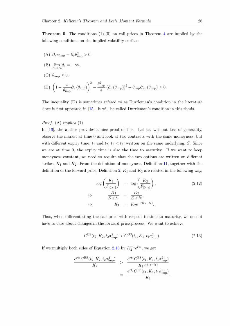
Theorem 5. The conditions (1)-(5) on call prices in Theorem 4 are implied by the
following conditions on the implied volatility surface:
(A) ∂τwimp = ∂τθ2imp > 0.
(B) limK→∞
d1 = −∞.
(C) θimp ≥ 0.
(D)
(1− x
θimp∂x (θimp)
)2
−θ2
imp
4(∂x (θimp))2 + θimp∂xx (θimp) ≥ 0.
The inequality (D) is sometimes refered to as Durrleman’s condition in the literature
since it first appeared in [15]. It will be called Durrleman’s condition in this thesis.
Proof. (A) implies (1)
In [16], the author provides a nice proof of this. Let us, without loss of generality,
observe the market at time 0 and look at two contracts with the same moneyness, but
with different expiry time, t1 and t2, t1 < t2, written on the same underlying, S. Since
we are at time 0, the expiry time is also the time to maturity. If we want to keep
moneyness constant, we need to require that the two options are written on different
strikes, K1 and K2. From the definition of moneyness, Definition 11, together with the
definition of the forward price, Definition 2, K1 and K2 are related in the following way,
log
(K1
F[0,t1]
)= log
(K2
F[0,t2]
), (2.12)
⇔ K1
S0ert1=
K2
S0ert2,
⇔ K1 = K2e−r(t2−t1).
Thus, when differentiating the call price with respect to time to maturity, we do not
have to care about changes in the forward price process. We want to achieve
CBS(t2,K2, t2σ2imp) > CBS(t1,K1, t1σ
2imp). (2.13)
If we multiply both sides of Equation 2.13 by K−12 ert2 , we get
ert2CBS(t2,K2, t2σ2imp)
K2>
ert2CBS(t1,K1, t1σ2imp)
K1er(t2−t1)
=ert1CBS(t1,K1, t1σ
2imp)
K1.

Chapter 2. Kellerer’s Theorem and Lee’s Moment Formula 27
Let the moneyness be constant. This implies that F[0,t]/K = e−x is also constant. Then
by Equation C.3, the function
f(wimp) =ertCBS(t,K,wimp)
K
=F[0,t]
KN (d1)−N (d2)
is an increasing function in total implied variance, wimp. Hence, if we assume ∂τwimp > 0,
then the call price CBS will be an increasing function in time to maturity.
(B) and (C) implies (2)
Since (2) follows if the Black call price goes to zero as the strike price goes to infinity,
we can examine the limit of CB instead of the limit of CBS. For the first term of CB,
that is FN (d1), note that only if we have condition (B),
limK→∞
d1(τ,K, τσ2imp) = lim
x→∞− x
θimp+θimp
2= −∞,
do we have N (d1(τ,K, τσ2imp)) → 0 as K → ∞. For the second term of CB, that is
KN (d2), note that
d2(τ,K, τσ2imp) = − x
θimp− θimp
2= −1
2
(2x
θimp+ θimp
). (2.14)
Recall the inequality of arithmetic and geometric means.
Lemma 1. (Arithmetic-Geometric inequality) For any set of n non-negative real num-
bers x1, . . . , xn, ∑ni=1 xin
≥ n
√√√√ n∏i=1
xi. (2.15)
Since we want to examine the limit when K tends to infinity, K can be assumed to
be positive in the following calculation. The forward price F is a price so it is always
positive and finite. These two facts together imply that for a large enough K, x will be
positive. If we assume that θimp(τ,K, τσ2imp) ≥ 0, Equation (2.15) applies to the right
hand side in Equation (2.14) and gives us
d2(τ,K, τσ2imp) = −1
2
(2x
θimp+ θimp
)≤ −
√2x
θimpθimp
= −√
2x.

Chapter 2. Kellerer’s Theorem and Lee’s Moment Formula 28
Note that since N is a probability distribution, it is an increasing function and therefore
0 ≤ exN(d2(τ,K, τσ2
imp))≤ exN
(−√
2x).
The right hand term tends to zero when K tends to infinity. The only condition that
we made on θimp here is that is condition (C), that it should be non-negative.
(D) implies (4)
In Equation (C.1), it is derived that
∂KKCBS = e−rτ∂KKC
B
=Sn(d1)
K2θimp
((1−√τx
θimp∂x (σimp)
)2
− τθ2
imp
4(∂x (σimp))2
+√τθimp∂xx (σimp)
).
Since S, n and θimp are non-negative and since θimp =√τσimp, the condition we need to
impose to ensure convexity of CBS in K is(1− x
θimp∂x (θimp)
)2
−θ2
imp
4(∂x (θimp))2 + θimp∂xx (θimp) ≥ 0, (2.16)
in order to insure the convexity of CB in K. Equation (2.16) can also be expressed in
terms of the total implied variance. The following relation is taken from Equation (C.2),
(1− x
2wimp∂x (wimp)
)2
− 1
4
(1
wimp+
1
4
)(∂x (wimp)
)2+
1
2∂xx (wimp) ≥ 0.
(B), (C) and (D) imply (3)
If (B), (C) and (D) hold then the call price is a convex, non-increasing function of K.
Since the call price is assumed to be twice differentiable, the following limit exists
limh→0
C(τ,K + h)− C(τ,K)
h. (2.17)
By Proposition 5 i), for all h > 0 the numerator satisfies
K − (K + h) ≤ C(τ,K + h)− C(τ,K) ≤ 0. (2.18)

Chapter 2. Kellerer’s Theorem and Lee’s Moment Formula 29
Applying Equation (2.18) and the definition of the partial derivative to Equation (2.17),
we get
−1 ≤ ∂KC(τ,K) ≤ 0.
A similar argument to that which was made in Theorem 2.1 of [12] can be done for the
previous inequality, leading to the limit
limK→−∞
∂KC(τ,K) + 1 = 0. (2.19)
Integrating Equation (2.19) with respect to K yields∫lim
K→−∞∂KC(τ,K) + 1 dK = a, a ∈ R.
Note that the explicit expression for the partial derivative is
∂KC(τ,K) =((St −K)+ + 1
)∂Kµτ (St).
Note furthermore that if we let fn be defined by
fn(K) =
((St −
1
n−K
)+
+ 1
)∂Kµτ (St),
then fn is a non-decreasing sequence of positive, measurable functions that converge
pointwise to ∂KC(τ,K). Hence the monotone convergence theorem is applicable and we
can move the limit outside the integral to obtain the result,
a =
∫lim
K→−∞∂KC(τ,K) + 1 dK
= limK→−∞
∫∂KC(τ,K) + 1 dK
= limK→−∞
C(τ,K) +K.
The Black-Scholes model implies (5)
The implied volatility is derived from the Black-Scholes model and therefore all assump-
tions of the Black-Scholes model will hold true for the implied volatility we calculate
using the model. The Black-Scholes call price formula is derived as the unique solution
to the Black-Scholes partial differential equation. This equation also has a call function
of the form which was introduced in Defintion 8 as solution by the discounted Feynman-
Kac theorem. Recall that a call function is an integral of a non-negative function with
respect to a probability measure. Therefore, the Black-Scholes model implies that the
call surface will be non-negative.

Chapter 2. Kellerer’s Theorem and Lee’s Moment Formula 30
2.5 Asymptotic bounds on the implied volatility smile
As was introduced in Definition 1, the implied volatility is the variable σimp that uniquely
solves
erτC(τ,K) = CB(τ,K, τσ2imp).
As before, let x denote the forward log-moneyness. Furthermore, let g(x) ∼ f(x) if
g(x)/f(x)→ 1 as x→∞.
The intuition behind the result of this section is that it is crucial to match the asymp-
totics of CB(τ,K, τσ2imp) with the asymptotics of C(τ,K), because if they are to agree
for all K, we need to have C ∼ CB. This forced matching will have implications on
the implied volatility. Let us investigate the limit behaviour of CB and C as K goes to
infinity and consolidate the intuition. As in many mathematical derivations, a special
function appears that suits our needs well,
f1(y) =
(1√y−√y
2
)2
,
f2(y) =
(1√y
+
√y
2
)2
.
Note that d1 and d2 can be expressed in terms of the functions f1 and f2,
d1(τ,K, τσ2imp) = −
(x
θimp− θimp
2
)= −
√x
(1
θimp/√x− θimp/
√x
2
)
= −√x
1√θ2
imp/x−
√θ2
imp/x
2
= −
√xf1(θ2
imp/x).
An analogous calculation can be made to show that
d2(τ,K, τσ2imp) = −
√xf2(θ2
imp/x).
With the functions f1 and f2 at hand, we get a nice expression of the Black call price
when σimp =√βx where β is a positive number,
CB(τ,K, τβx) = F(N (−
√xf1(β))− exN (−
√xf2(β))
). (2.20)

Chapter 2. Kellerer’s Theorem and Lee’s Moment Formula 31
Since we want to investigate the limit when K goes to positive infinity, we may without
loss of generality assume that βx > 0 and the implied volatility in Equation (2.20) is
therefore well defined. Equation (2.20) allows us to study the asymptotics of the Black
call price when the implied variance is linear in moneyness. Through partial integration
an asymptotic approximation can be derived for N (y). Using the fact that ∂yN (y) is
an even function,
N (−y) =1√2π
∫ −y−∞
e−t2/2 dt
=1√2π
∫ ∞y
e−t2/2 dt
=1√2π
∫ ∞y2/2
s−1/2e−s ds
=1√2π
(e−y
2/2
y− 1
2
∫ ∞y2/2
s−3/2e−s ds
).
Since both s−3/2 and e−s are decreasing functions on[y2/2,∞
), the integral on the right
hand side can be bounded,∣∣∣∣∣∫ ∞y2/2
s−3/2e−s ds
∣∣∣∣∣ ≤ 1
y3
∫ ∞x2/2
e−s ds
≤ e−y2/2
y3.
Hence we have that
N (−y) ∼ e−y2/2
y√
2π, y →∞. (2.21)
Using that f1(β) + 2 = f2(β) together with the asymptotics from Equation (2.21), the
asymptotics of CB can be retrieved,
CB(τ,K, τβx) = F(N (−
√xf1(β))− exN (−
√xf2(β))
)∼ F√
2π
(e−xf1(β)/2√xf1(β)
− exe−xf2(β)/2√xf2(β)
)
=F√2πx
(e−xf1(β)/2√
f1(β)− exe−x(f1(β)+2)/2√
f2(β)
)
=e−xf1(β)/2
B(β)√x.
Here B is a function depending only on β. Having established the asymptotic properties
for CB for large strikes, now we need to do the same for C. Recall from Section 2.3
C(τ,K) = E[(St −K)+],
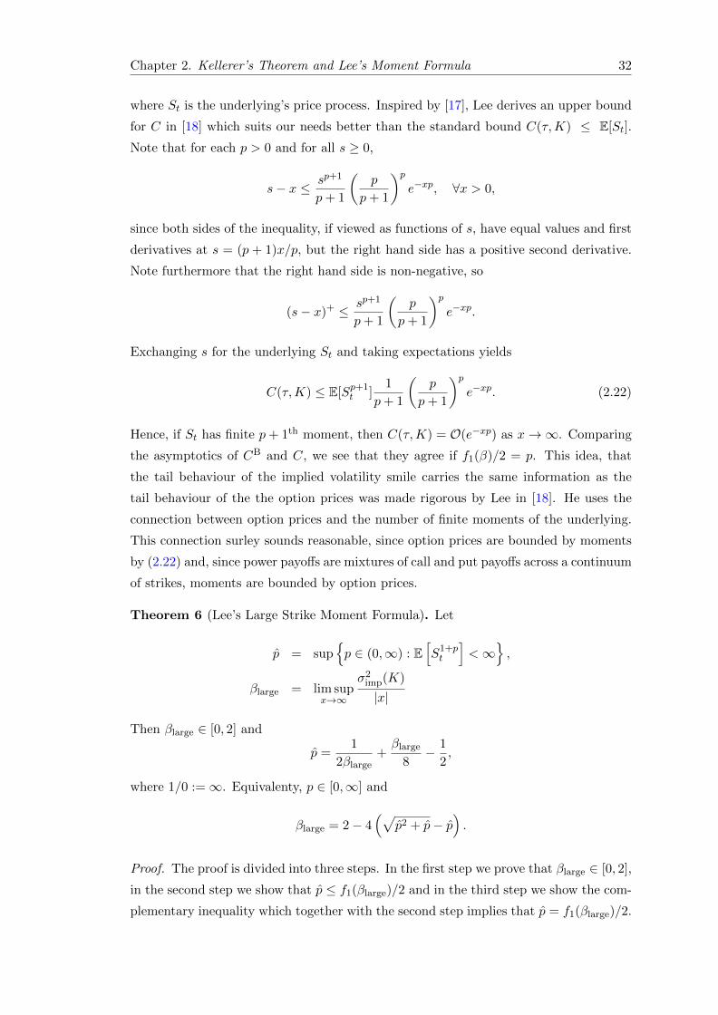
Chapter 2. Kellerer’s Theorem and Lee’s Moment Formula 32
where St is the underlying’s price process. Inspired by [17], Lee derives an upper bound
for C in [18] which suits our needs better than the standard bound C(τ,K) ≤ E[St].
Note that for each p > 0 and for all s ≥ 0,
s− x ≤ sp+1
p+ 1
(p
p+ 1
)pe−xp, ∀x > 0,
since both sides of the inequality, if viewed as functions of s, have equal values and first
derivatives at s = (p + 1)x/p, but the right hand side has a positive second derivative.
Note furthermore that the right hand side is non-negative, so
(s− x)+ ≤ sp+1
p+ 1
(p
p+ 1
)pe−xp.
Exchanging s for the underlying St and taking expectations yields
C(τ,K) ≤ E[Sp+1t ]
1
p+ 1
(p
p+ 1
)pe−xp. (2.22)
Hence, if St has finite p+ 1th moment, then C(τ,K) = O(e−xp) as x→∞. Comparing
the asymptotics of CB and C, we see that they agree if f1(β)/2 = p. This idea, that
the tail behaviour of the implied volatility smile carries the same information as the
tail behaviour of the the option prices was made rigorous by Lee in [18]. He uses the
connection between option prices and the number of finite moments of the underlying.
This connection surley sounds reasonable, since option prices are bounded by moments
by (2.22) and, since power payoffs are mixtures of call and put payoffs across a continuum
of strikes, moments are bounded by option prices.
Theorem 6 (Lee’s Large Strike Moment Formula). Let
p = supp ∈ (0,∞) : E
[S1+pt
]<∞
,
βlarge = lim supx→∞
σ2imp(K)
|x|
Then βlarge ∈ [0, 2] and
p =1
2βlarge+βlarge
8− 1
2,
where 1/0 :=∞. Equivalenty, p ∈ [0,∞] and
βlarge = 2− 4(√
p2 + p− p).
Proof. The proof is divided into three steps. In the first step we prove that βlarge ∈ [0, 2],
in the second step we show that p ≤ f1(βlarge)/2 and in the third step we show the com-
plementary inequality which together with the second step implies that p = f1(βlarge)/2.

Chapter 2. Kellerer’s Theorem and Lee’s Moment Formula 33
Step 1. If there exists an x > 0 such that for all x > x,
σimp <√
2|x|,
then by the definition of βlarge in the theorem statement, βlarge ∈ [0, 2]. This is equivalent
to
CB(τ,K, τσ2imp) < CB(τ,K, τ2|x|), x > x, (2.23)
since CB is strictly increasing in the first argument. We know from the definition of
implied volatility that the left hand side of (2.23) is equal to C(τ,K) = E [(St −K)+].
Now (St −K)+x>0 is a family of non-negative random variables that converge to 0 as
x goes to infinity and are bounded from above by Sτ . Furthermore, E[St] <∞ since we
have assumed that the call prices exist. Then, by dominated converge,
limx→∞
C(τ,K) = limx→∞
E[(Sτ −K)+
]= 0.
For the right hand side of (2.23), note that
CB(τ,K, τ2|x|) = F(N (0)− exN (−
√2|x|)
)= F
(1
2− exN (−
√2|x|)
).
By l’Hopital’s rule,
limx→∞
N (−√
2|x|)e−x
= limx→∞
2(2|x|)−1/2e−(−√
2|x|)2/2
e−x= lim
x→∞
√2e−x√|x|e−x
= 0,
so
limx→∞
CB(τ,K, τ2|x|) =F
2,
and the first step of the proof is finished.

Chapter 2. Kellerer’s Theorem and Lee’s Moment Formula 34
Step 2. In the this and the third step, we need a special limit. For β ∈ (0, 2) and a
constant c,
limx→∞
e−cx
CB(τ,K, τβ|x|)= lim
x→∞
e−cx
F(N (−
√xf1(β))− exN (−
√xf2(β))
)= lim
x→∞
ce−cx
F
(n(−√xf1(β)
)√f1(β)
x− exn
(−√xf2(β)
)√f2(β)
x
)
= limx→∞
ce−cx
F
(e−xf1(β)/2
√f1(β)
x− exe−xf2(β)/2
√f2(β)
x
)
= limx→∞
ce−cx
F
(e−xf1(β)/2
(√f1(β)
x−√f2(β)
x
))
= limx→∞
c
F
( √x√
f1(β)−√f2(β)
)ex(f1(β)/2−c)
=
0, c > f1(β)/2,
∞, c ≤ f1(β)/2.
Let β ∈ (0, 2) and p ∈ (f1(β)/2, p) where p is defined as in the theorem statement. By
(2.22) and the previous limit we have that when x→∞,
CB(τ,K, τσ2imp)
CB(τ,K, τβ|x|)=
O(e−px)
CB(τ,K, τβ|x|)→ 0. (2.24)
Note now that f1(β) is strictly decreasing when β ∈ (0, 2). This implies that for
any β ∈ (0, 2) with f1(β)/2 < p, we have βlarge ≤ β and hence we need to have
p ≤ f1(βlarge)/2 in order for the limit (2.24) to be a constant.
In the case when this last step is vacuously true, that is if there exists no β ∈ (0, 2)
such that f1(β)/2 < p, we have by the definition in the statement of the theorem that
βlarge = 0 and p = f1(βlarge)/2 =∞.

Chapter 2. Kellerer’s Theorem and Lee’s Moment Formula 35
Step 3. In this step we will prove the complementary inequality, p ≥ f1(βlarge)/2. From
the defintion of p, we see that it is enough to show that for any p ∈ (0, f1(βlarge)/2),
E[S1+pτ
]is finite. To show this, we pick β such that f1(β)/2 ∈ (p, f1(βlarge)). Then, as
earlier, for large enough x,
C(τ,K)
e−xf1(β)/2≤ CB(τ,K, τβ|x|)
e−xf1(β)/2→ 0, as x→∞.
Thus there exists a K∗ so that for K > K∗, C(τ,K) < K−f1(β)/2. Using the spanning
relation from Appendix B with k = 0, we have
E[Sp+1t
]= E
[∫ ∞0
(p+ 1)pKp−1(St −K)+dK
]≤ (p+ 1)p
[∫ K∗
0Kp−1C(τ,K)dK +
∫ ∞K∗
Kp−1−f1(β)/2dK
]<∞.
There is a corresponding theorem for small strikes. An analogous proof as the one for
the large strike formula can be done, but a shorter one was presented in [19] that builds
on what we already know from the large strike formula. Since the proofs are similar to
a great extent, the proof is omitted.
Theorem 7 (Lee’s Small Strike Moment Formula). Let
q = supq ∈ (0,∞) : E
[S−qt
]<∞
,
βsmall = lim supx→−∞
σ2imp(K)
|x|t.
Then βsmall ∈ [0, 2] and
q =1
2βsmall+βsmall
8− 1
2,
where 1/0 :=∞. Equivalently, q ∈ [0,∞] and
βsmall = 2− 4(√
q2 + q − q).
The implications on the characteristics of implied volatility from Theorem 6 and Theo-
rem 7 are important. The theorems determine that the implied volatility cannot grow
faster than√|x|. That is, for large enough |x|, σimp has to be smaller or equal to
√β|x|.
Furthermore, unless St has finite moments of all orders which corresponds to the case
where β = 0, the implied volatility cannot grow slower than√|x|.

Chapter 3
Parameterization of the implied
volatility
A parametric model of the implied volatility comes with certain advantages. Observed
implied volatilities, and hence call prices, can be inter- and extrapolated. Therefore a
parametric implied volatility model can be used to price new contracts for which there
are no quotes on the market. The implied volatility in a parametric model is function
of strike and maturity with an explicit analytical expression. If the implied volatility
is modeled as a smooth function it will also admit analytical explicit expression for its
derivatives of all orders possibly saving computational time. A parametric model have
to satisfy the conditions derived in Chapter 2 to be considered as feasible.
There exist several popular models for stochastic implied volatility, with the most popu-
lar being Stochastic Volatility Inspired (SVI) parameterization [1], the Stochastic alpha,
beta, rho (SABR) parameterization [20] and Vanna-Volga (VV) model. We are con-
cerned with the SVI, but it could be of some interest to mention some properties and
limitations of the other models.
This chapter starts with a short examination of the three mentioned models. After
this follows a summary of the different variations of the SVI parameterization that were
introduced in [2] together with their interpretation. Finally, this chapter ends with a
summary of the work in [2] that treats conditions on the SVI parameters that guarantee
the absence of static abitrage in the implied volatility they define.
36

Chapter 3. Parameterization of the implied volatility 37
3.1 Popular stochastic volatility models
Stochastic volatility inspired (SVI)
The SVI parameterization of the total implied variance for a fixed time to maturity
reads,
wSVIimp(x) = a+ b
(ρ(x−m) +
√(x−m)2 + σ2
), (3.1)
where x is moneyness and a, b, σ, ρ,m is the parameter set. The SVI parameter σ
is not to be confused with the volatility of the underlying’s price process, which is also
denoted by σ! The first strength of the SVI is demonstrated in the following proposition.
Proposition 8. The SVI parameterization in Equation (3.1) satisfies Lee’s large and
small strike formulas.
Proof. The right asymptote is by [1]
(wSVI
imp
)r
(x) = a+ b(1− ρ)(x−m).
The left asymptote is by [1]
(wSVI
imp
)l(x) = a− b(1 + ρ)(x−m).
They are both linear in moneyness hence satisfy Lee’s formula.
Note that these asymptotes imply through Lee’s large and small strike formulas that
the distribution of the underlying’s price process has finite moments of all orders. This
is a model limitation of the SVI, since by [19] the implied volatility may grow slower
than√x when the distribution on the underlying’s price process does not have finite
moments of all orders, because of for example fat tails. Work such as [21] and [22] tries
to solve this by introducing more parameters into Equation (3.1), but these two models
and their implementation is outside the area of interest for this thesis.
The second strength of the SVI model was established in [23]. It was shown that the
implied volatility in the Heston model converges to the SVI in the long maturity limit.
The Heston model assumes the same dynamics for the implied variance as was done in
Chapter 2.1, but assigns the coefficients in Equation (2.6). The implied variance in the
Heston model follows the dynamics
dvimp = θ(ω − vimp)dt+ η√vimpdB1
t . (3.2)

Chapter 3. Parameterization of the implied volatility 38
Here, ω is a long-time mean value of the variance and θ is the rate at which the variance
reverts towards ω. The volatility of the variance process is η. This choice of dynamics
is built on three assumptions, namely that the variance of S is a random process that
1. has a tendency to revert towards its long-term mean at some constant rate,
2. has a volatility that is proportional to the square root of its level,
3. has a source of randomness that is correlated with the randomness of the under-
lying’s price process.
The assumption about mean reversion is often deemed as being the cause of mean re-
version. If traders believe in the assumption of mean reversion, then traders will sell
contracts when they are worth more than the long-term mean and buy when the con-
tracts are worth less than the long term mean. Through their actions on the market,
the traders will cause mean reversion.
The second assumption can be motivated by the observation of volatility clustering.
In Figure 3.1 daily returns for the S&P 500 index are plotted. It is visible that larger
movements cluster together and are interupted by periods of smaller movements. Heuris-
tically, we see that the size of the movements depends on the size of the movements.
The third assumption was motivated in Chapter 2.1.
Stochastic alpha, beta, rho (SABR)
The underlying’s price process is in the SABR modeled with the following dynamics,
dSt = σtSβt dB0
t ,
dσt = ασtdB1t ,
〈dB0t , dB
1t 〉 = ρdt,
where B0 and B1 are standard Brownian motions, β ∈ [0, 1] is a skewness parameter,
α ≥ 0 is the volatility of volatility and ρ ∈ [−1, 1]. A flaw in the SABR model is the lack
of mean reversion, which makes it suitable for options with short time to maturity only.
A strength of the SABR model is that it yeilds an explicit formula in the short time
to maturity limit, which makes it possible to fit the parameters β, α and ρ to market
data. The retrieved function with the fitted parameters can then be expanded using
Taylor’s formula to yield approximate implied volatilities to options with non-zero, but
short, times to maturity. This is done for example in [1]. The SABR model is especially
popular in the interest rate derivative markets.

Chapter 3. Parameterization of the implied volatility 39
0 2000 4000 6000 8000 10000 12000 14000 16000 18000−0.25
−0.2
−0.15
−0.1
−0.05
0
0.05
0.1
0.15S&P 500 daily log returns from 1950 until today.
Days after 3rd of January 1950
Dai
ly lo
g re
turn
Figure 3.1: The daily log returns of S&P 500 from January 3rd 1950 until today. Aslight clustering is visible. Data from finance.yahoo.com/ on 7/14/2014.
Vanna-Volga (VV)
The VV model is not based on assumptions on the underlying’s price process but on
a hedge of three big risks associated with the volatility of an option. The three risks
are called vega, vanna and volga in the finance lingo. The vega is the sensitivity of the
option value towards a change in implied volatility, the vanna is the sensitivity of the
vega with respect to a change in the underlying’s price process and finally the volga is
the sensitivity of the vega with respect to changes in the implied volatility. A portfolio
which hedges these three risks is created, and the Black-Scholes value of the option is
adjusted by the value of this portfolio. The implied volatility can then be found by an
inversion. The procedure is thoroughly explained in [24]. In [24], it is mentioned that
the VV model does not guarantee convexity of the call prices, thus exposing the model
to static arbitrage. The VV model is popular in the foreign exchange market.

Chapter 3. Parameterization of the implied volatility 40
3.2 SVI parametrizations and their interpretation
In [2], three equivalent versions of the SVI parameterization in Equation 3.1 are intro-
duced; the raw, the natural and the jump-wing.
Natural parametrization
The natural parametrization of the SVI total implied variance reads
wSVIimp(x) = ∆ +
ω
2
(1 + ηρ(x− µ) +
√(η(x− µ) + ρ)2 + (1− ρ2)
).
The natural parameterization is the functional form that appears as the limit of the
Heston model. Unaesthetic expressions of ω and η in terms of the Heston parameters
from Equation 3.2 can be found in [23], while ρ is simply the correlation between the
Brownian motions driving the underlying’s price process and the variance process and
∆ and µ are vertical and horizontal shifts respectively. The natural parameterization is
not as useful implementationwise as the two subsequent parameterizations.
Raw parametrization
The raw parametrization of SVI total implied variance reads
wSVIimp(x) = a+ b
(ρ(x−m) +
√(x−m)2 + σ2
).
This is the most frequently used version of the SVI parameterization in the litterature
and it is also the original parameterization, introduced first in [1]. The effects on the
volatility smile of the raw parameters are listed below:
• Increasing a results in a vertical translation of the smile in the positive direction.
• Increasing b decreases the angle between the put and call wing, i.e. tightens the
smile.
• Increasing ρ results in a counter-clockwise rotation of the smile.
• Increasingm results in a horizontal translation of the smile in the positive direction.
• Increasing σ reduces the at-the-money curvature of the smile.
At-the-money is the financial term for the point x = 0, the point where the strike price is
equal to the forward price. These properties of the raw parameters have been visualized
in many articles, for example in [1].

Chapter 3. Parameterization of the implied volatility 41
Having bounds on the feasible region of these parameters is very useful when imple-
menting the SVI model, since we will eventually have to do an optimization to find
the, in some sense, best parameter set for an input data set. From the properties listed
above, some obvious bounds for the raw parameters can be deduced. First of all, it is
an empirical fact that volatility smiles have a positive at-the-money curvature. Hence
we impose
σ > 0. (3.3)
This bound has also computational advatages that will become clear to the reader in
Chapter 4.3. The same fact also forces us to impose
b ≥ 0. (3.4)
Furthermore, we dont want an optimal parameter set to give a total implied variance
curve that is systematically greater than the largest observed total variance. If wi are
the observed total variances we want to fit our SVI to, we impose
a ≤ maxiwi. (3.5)
By the same reasoning, if xi are the moneynesses corresponding to the observed total
variances, we impose
m ≥ 2minixi, (3.6)
m ≤ 2maxixi. (3.7)
Finally, since ρ is the correlation between the Brownian motions driving the underlying’s
price process and the underlying’s variance process we need to have
ρ ∈ [−1, 1]. (3.8)
More bounds will be derived in Chapter 4.3, but from a more analytical point of view.
A final note about the raw parameters is that they relate to the natural parameters in
the following way,
(a, b, ρ,m, σ) =
(∆ +
ω
2(1− ρ2),
ωη
2, ρ, µ− ρ
η,
√1− ρ2
η
),
(∆, µ, ρ, ω, η) =
(a− ω
2(1− ρ2),m+
ρσ√1− ρ2
, ρ,2bσ√1− ρ2
,
√1− ρ2
σ
).
These relations give the possibility of an interpretation of the raw parameters in terms
of the Heston model parameters.

Chapter 3. Parameterization of the implied volatility 42
Jump-Wing (JW) parameterization
The JW parameterization is defined in terms of the raw parameters,
vτ =a+ b
(−ρm+
√m2 + σ2
)τ
, (3.9)
ψτ =1√wτ
b
2
(ρ− m√
m2 + σ2
),
pτ =1√wτb(1− ρ),
cτ =1√wτbt(1 + ρ),
vτ =1
τ
(a+ bσ
√1− ρ2
),
where wτ = vττ . Note that this parameterization depends explicitly on the time to
maturity, τ . In [2], an inversion formula for Equation (3.9) is presented. The parameters
are more tractable for traders than the two previous parameterization. More importantly
for the aim of this thesis, there is literature on how to find conditions on them to prevent
static arbitrage in the implied volatility surface. That will be the topic of Chapter 3.3.
The tractability comes from the interpretations of the parameters, which are presented
below.
• vτ is the at-the-money implied variance. This is easily seen, since in the raw
parameterization vτ = wSVIimp(x)/τ
∣∣∣x=0
.
• ψτ is the at-the-money implied volatility skew. This requires some calculation,
∂x
√wSVI
imp(x)
τ
∣∣∣∣∣∣x=0
=1
2√wSVI
imp(x)τ
∣∣∣∣∣∣x=0
∂xw(x)|x=0
=1
2√vττ
b
(ρ+
2x− 2m
2√
(x−m)2 + σ2
)∣∣∣∣∣x=0
=1√wτ
b
2
(ρ− m√
m2 + σ2
)= ψτ .
• pτ is the slope of the left wing, the part of the smile corresponding to out-of-the-
money put options, scaled with the at-the-money total implied volatility,
limx→−∞
wSVIimp(x)
x= lim
x→−∞
1
x
(a+ b
(ρ(x−m) +
√(x−m)2 + σ2
))= lim
x→−∞
a
x+ b
(ρ(
1 +m
x
)+
√(1 +
m
x
)2+(σx
)2)
= b(ρ+ 1) = pτ√wτ

Chapter 3. Parameterization of the implied volatility 43
• cτ is the slope of the right wing, the part of the smile corresponding to out-of-
the-money call options, scaled with the at-the-money total implied volatility. The
calculation is analoguous to that for pτ .
• vτ is the minimum level implied variance. This was seen in the examination of the
raw parameters.
3.3 The restriction: SSVI
We begin this section by introducing two standard definitions from the literature. Recall
the conditions from Theorem 5.
Definition 15 (Butterfly arbitrage). For a fixed and positive real τ , the implied volatil-
ity smile σimp(τ,K)|τ=τ0is free of butterfly arbitrage if and only if conditions (B) and
(D) from Theorem 5 are satisfied.
Definition 16 (Calendar spread arbitrage). An implied volatility surface σimp(τ,K) is
free of calendar spread arbitrage if and only if condition (A) from Theorem 5 is satisfied.
Together with condition (C) from Theorem 5, absence of butterfly and calendar spread
arbitrage is equivalent to absence of static arbitrage. As was discussed in the proof of
Theorem 5, condition (C) will always be satisfied since we are using the implied volatility
implied by the Black-Scholes call price formula.
With a parameterization, we could now calibrate the parameters to fit input volatil-
ity data, but we would like to do this in such a way that the output call prices are free
of static arbitrage. In literature such as [2] and [25], the authors express hopelessness
in front of the task to state conditions for the SVI parameters in order to guarantee
no butterfly arbitrage. On the other hand, the easiness of eliminating calendar spread
arbitrage is pronounced as a great strenth of the SVI model. The problem with butterfly
arbitrage was partly solved in [2] where the authors propose a new parameterization for
the total implied variance which they name Surface SVI (SSVI),
wSSVIimp (τ, x) =
θτ2
(1 + ρxφ(θτ ) +
√(xφ(θτ ) + ρ)2 + (1− ρ2)
).
The requirements on the new parameters θt and φ are that θt has to be positive and
φ has to be a smooth function from (0,∞) to [0,∞). As earlier, ρ can take values
in [−1, 1]. Note that the SSVI parameterization is the natural parameterization with
its parameters restricted as (∆, µ, ρ, ω, η) = (0, 0, ρ, θt, φ(θt)). Hence, the number of

Chapter 3. Parameterization of the implied volatility 44
variables that the parameterization depends on has gone down from five to three. Note
also that θt is the at-the-money total implied variance.
Proposition 9. The JW parameters corresponding to the SSVI are
vt = θt/t,
ψt =1
2ρ√θtφ(θt),
pt =1
2
√θtφ(θt)(1− ρ),
ct =1
2
√θtφ(θt)(1 + ρ),
vt =θtt
(1− ρ2
).
Proof. In the calculations below, text under the equality sign denotes change of param-
eterization. The leftmost term is always stated in the JW parameterization.
vt =Raw
1
t
(a+ b
(−ρm+
√m2 + σ2
))=
Natural
1
t
∆ +ω
2
(1− ρ2
)+ωη
2
−ρ(µ− ρ
η
)+
√√√√(µ− ρ
η
)2
+
(√1 + ρ2
η
)2
=SSVI
1
t
(θt2
(1− ρ2
)+θtφ(θt)
2
(ρ2
φ(θt)+
√ρ2
φ(θt)2+
1 + ρ2
φ(θt)2
))
=1
t
(θt2− θtρ
2
2+θtρ
2
2+θt2
)=θtt,
ψt =Raw
1√wt
b
2
(ρ− m√
m2 + σ2
)
=Natural
1√vtt
ωη
4
ρ− µ− ρη√(
µ− ρη
)2+(√
1−ρη
)2
=
SSVI
1√θt
θtφ(θt)
4
ρ+ρ
φ(θt)√
ρ2
φ(θt)2+ 1−ρ2
φ(θt)2
=
1
2ρ√θtφ(θt),

Chapter 3. Parameterization of the implied volatility 45
pt =Raw
1√wtb(1− ρ)
=Natural
1√vtt
ωη
2(1− ρ)
=SSVI
1√θt
θtφ(θt)
2(1− ρ)
=1
2
√θtφ(θt)(1− ρ),
ct =Raw
1√wtb(1 + ρ)
=SSVI
1
2
√θtφ(θt)(1 + ρ),
v =Raw
1
t
(a+ bσ
√1− ρ2
)=
Natural
1
t
(∆ +
ω
2(1− ρ2) +
ωη
2
√1− ρ2
η
√1− ρ2
)=
1
t
(∆ + ω(1− ρ2)
)=
SSVI
θtt
(1− ρ2).
Using the SSVI, sufficient conditions for absence of static arbitrage are stated in [2].
Theorem 8. The SSVI is free of butterfly arbitrage if
(1) θτφ(θτ ) (1 + |ρ|) < 4,
(2) θτφ(θτ )2 (1 + |ρ|) ≤ 4.
Proof. The proof is omitted. It is based on a rewriting of condition (D) of Theorem 5,
Durrleman’s condition, and can be found in [2].
Theorem 9. The SSVI is free of calendar spread arbitrage if and only if
(1) ∂τθτ ≥ 0,
(2) 0 ≤ ∂θτ(θτφ(θτ )
)≤ 1
ρ2
(1 +
√1− ρ2
)φ(θτ ).
Proof. The proof is omitted. It is based on a rewriting of condition (A) of Theorem 5,
∂τwimp ≥ 0, and can be found in [2].

Chapter 3. Parameterization of the implied volatility 46
Using Proposition 9, Theorem 8 can be translated into the JW parameterization.
Proposition 10. The SSVI is free of butterfly arbitrage if
(1)√vττ max(pτ , cτ ) < 2,
(2) (pτ + cτ ) max(pτ , cτ ) ≤ 2.
Proof. Note that (1 + |ρ|) < a if and only if max(1 − ρ, 1 + ρ
)< a. Using this, (1) is
given by
√vττ max(pτ , cτ ) =
√θτ max
(1
2
√θτφ (θτ ) (1− ρ),
1
2
√θτφ (θτ ) (1 + ρ)
)=
θτφ(θτ )
2max
(1− ρ, 1 + ρ),
and (2) is given by
(pτ + cτ ) max(pτ , cτ ) =1
2
√θτφ(θτ )(1− ρ+ 1 + ρ)
√θτφ(θτ )
2max
(1− ρ, 1 + ρ)
=θτφ(θτ )2
2max(1− ρ, 1 + ρ).
Suppose that we have calibrated an SVI to some input data and know the calibrated
JW parameters. Then [2] tells us that if we fix the JW parameters vτ , ψτ and pτ of this
smile and the repick cτ and vτ as
cτ = pτ + 2ψτ , (3.10)
vτ = vτ4pτ cτ
(pτ + cτ )2 , (3.11)
then by Proposition 10 we are guaranteed to have a smile that is free of butterfly
arbitrage. Another way to do this is to fix vτ , ψτ and cτ and the repick pτ and vτ
using Equation (3.10) and Equation (3.11). This result will be a main component in the
calibration algorithm, which is presented in the next chapter.

Chapter 4
Parameter calibration
In this chapter a method to calibrate the SVI parameters to market data will be pre-
sented. The line of work is close to, and inspired by, the work of [26] and [27]. First,
the parameter bounds of Chapter 3.2 are complemented so that we have a lower and
an upper bound for all the raw parameters. Then a new parameterization, called the
Quasi-Explicit parameterization, is introduced. Finally the necessary optimization is
reviewed and the calibration algorithm is summarized. Related to this chapter is Ap-
pendix A where the optimization algorithm that was used, the Nelder-Mead method, is
described.
4.1 More parameter bounds
Recall the raw SVI parameterization of the total implied variance,
wSVIimp(x) = a+ b
(ρ(x−m) +
√(x−m)2 + σ2
).
If ρ2 6= 1, then wSVIimp(x) has the unique minimum a+ bσ
√1− ρ2. If ρ = 1, then wSVI
imp(x)
is non-decreasing and if ρ = −1, then wSVIimp(x) is non-increasing.
If σ goes to 0, then wSVIimp(x) becomes a piecewise affine function of the form c1x+c2. This
will cause the calibration to be an ill-posed problem. An example from [26] illuminates
this. If we let σ go to 0 and let m be greater than the largest observed moneyness then
c1 = b(ρ− 1),
c2 = a− bm(ρ− 1),
which leaves us with infinitely many choices of the triplet (a, b, ρ). Some bounds have to
be imposed to prevent an optimization algorithm to get stuck. To make a good decision
47

Chapter 4. Parameter calibration 48
we need to take a look at another case. Let σ go to infinity and let at the same time a
go to negative infinity. Using a Taylor expansion and the ∼ notation from Chapter 2.5,
we get for large σ and negative a that
wSVIimp(x) = a+ b
(ρ(x−m) +
√(x−m)2 + σ2
)= −|a|+ bρ(x−m) + bσ
√1 +
(x−mσ
)∼ −|a|+ bρ(x−m) + bσ
(1 +
1
2
(x−mσ
)).
Letting |a| = bσ, we get
limσ→∞a→−∞|a|=bσ
wSVIimp(x) = bρ(x−m).
In this affine smile, we can find bρ and m, but not the triplet (b, ρ,m) uniquely. To solve
these problems above, and gain stability in an optimization, we set a lower bound for a,
a ≥ 0, (4.1)
and reset the lower bound for σ from Equation 3.3,
σ ≥ σmin > 0. (4.2)
The value of σmin is a user choice, but should be picked to be very small in comparison
to typical parameter values.
No upper bound can be derived for σ, but a small integer always does the job. An
implementation using for example
σ ≤ 10 (4.3)
would certainly cover all smiles appearing from market input data since such a large σ
lifts the whole smile above 100% total implied variance, but if computer power is the
limitation a smaller integer such as 1 is also a good choice for the upper bound.
In [28] the authors derive a necessary condition for the absence of dynamic arbitrage for
the total implied variance that reads
|∂xwimp(x)| ≤ 4, ∀x, ∀τ.

Chapter 4. Parameter calibration 49
This is a condition that is widely used in the SVI literature, because it yields an upper
bound for b,
b ≤ 4
τ (1 + |ρ|). (4.4)
Let us end this section with a summary of all bounds that we have derived for the raw
parameters:
0 ≤ a ≤ maxiwi, (4.5)
0 ≤ b ≤ 4
τ (1 + |ρ|),
−1 ≤ ρ ≤ 1,
minixi ≤ m ≤ max
ixi,
0 < σmin ≤ σ ≤ 10 (or another ”large” number).
4.2 A new parameterization
The more parameters to calibrate, the more computing power is needed to do each
optimization. In the SVI model there are 5 parameters and if a dimension reduction
was possible it would speed up the calibration of the SVI. An observation in this line of
though was made in [26]. Let
y(x) =x−mσ
.
Under this change of variables, the total implied variance in the raw parameterization
reads,
wSVIimp(x) = a+ bσ
(ρy(x) +
√y(x)2 + 1
)(4.6)
= a+ dy(x) + cz(x),
where
a = a, d = ρbσ,
c = bσ, z(x) =√y(x)2 + 1.
Observe that given a value of (σ,m), wSVIimp(x) in Equation (4.6) depends linearly on
a, d, c. This ”split” of the parameter set, into a linear and a non-linear part, will be
extremely useful in the optimization that is to follow. The parameterization in Equa-
tion (4.6) will henceforth be refered to as the Quasi-Explicit (QE) parameterization,
inspired by the name of the paper where it was first defined.

Chapter 4. Parameter calibration 50
The parameters a, d, c will from now on be refered to as the inner parameters and σ,m
as the outer parameters.
Before we move on to the optimization, a word of caution to anyone who wants to
implement this. In the article [26], the authors have incorrectly stated that wSVIimp is the
implied variance, instead of the total implied variance. Therefore, they have an extra τ
factor throughout the paper.
4.3 Optimization
Translating the ten bounds in Equation 4.5 into bounds for the inner parameters a, d, c
in the Quasi-Explicit parameterization, we see that the triplet (a, d, c) has a compact
and convex domain in R3,
D =
(a, d, c) :
0 ≤ c ≤ 4σ
|d| ≤ c|d| ≤ 4σ − c0 ≤ a ≤ max
iwi
,
where wi is as in Equation (3.5) the input set of observed total variances. For a fixed
pair (σ,m), we are facing the optimization
min(a,d,c)∈D
fxi,wi(a, d, c), (4.7)
where fxi,wi is the quadratic cost function,
fxi,wi(a, d, c) =n∑i=1
(a+ dy(xi) + cz(xi)− wi)2 .
Note that fxi,wi is a smooth and convex function. Hence by a standad theorem from
calculus, f has a unique minimum for every fixed (σ,m) on the convex and compact
set D. Furthermore, the gradient of f is linear in (a, d, c), so the solution can easily
be computed analytically by calculating the inverse of a 3 × 3 equation system. This
makes it possible to do an extremely fast optimization of the inner parameters given
the outer parameters. A smart optimization algorithm should take advantage of this
and involve an ”outer optimization” that optimizes (σ,m) and an ”inner optimization”,
that in every step of the outer optimization optimizes (a, d, c) over D. Let (a∗, d∗, c∗) be
the solution of Equation (4.7) and let (a∗, b∗, ρ∗) be the corresponding raw parameters.

Chapter 4. Parameter calibration 51
Then the whole optimization can be stated as
min(σ,m)∈E
n∑i=1
(w(a∗,b∗,σ,ρ∗,m) − wi
)2, (4.8)
where E is the domain of (σ,m). The situation for the outer optimization is not as bright
as for the inner. First of all, fxi,wi depends non-linearly on (σ,m). Secondly, fxi,wi usu-
ally has multiple minima which makes gradient methods unreliable. An optimizer that
can work around these concerns is the Nelder-Mead method with probabilistic restarts.
It is treated in detail in Appendix A.
When we have arrived to a optimal set of raw parameters, we can check if this set
gives an implied volatility smile that is free of static arbitrage by checking if it satisfies
Durlemann’s condition an condition (B) from Theorem 5. In [28], it is shown that (B)
is equivalent to call prices tending to zero in the large strike limit, which is always the
case in observed data. Therefore, it is sufficient to check Durrleman’s condition. If the
implied volatility smile satisfies it, the calibration is complete. If it does not a recalibra-
tion is needed. This is the second step of the optimization. By translating the calibrated
parameters from raw to JW, we get a JW parameter set (vτ , ψτ , pτ , cτ , vτ ) that admits
static arbitrage. We can then use Equation 3.10 and Equation 3.11 to repick cτ and vτ
and retrieve a new JW parameter set (vτ , ψτ , pτ , c′τ , v′τ ) which defines an implied volatil-
ity smile that is guaranteed to be free of static arbitrage. Now observe that Durrleman’s
condition is a continuous function of the parameters cτ and vτ . This guarantees us to
find a solution to the optimization
min(cτ ,vτ )∈[cτ ,c′τ ]×[vτ ,v′τ ]
(wSVI
imp(x; cτ , vτ )− wSVIimp(x; cτ , vτ )
)2, (4.9)
such that Durrleman’s condition is satisfied.
The optimization (4.9) yields, in a sense, the SVI closest to the originally calibrated SVI
that is free of static arbitrage. Since we may encounter multiple minima and non linear-
lity here aswell, the Nelder-Mead method can be implemented to solve this optimization.
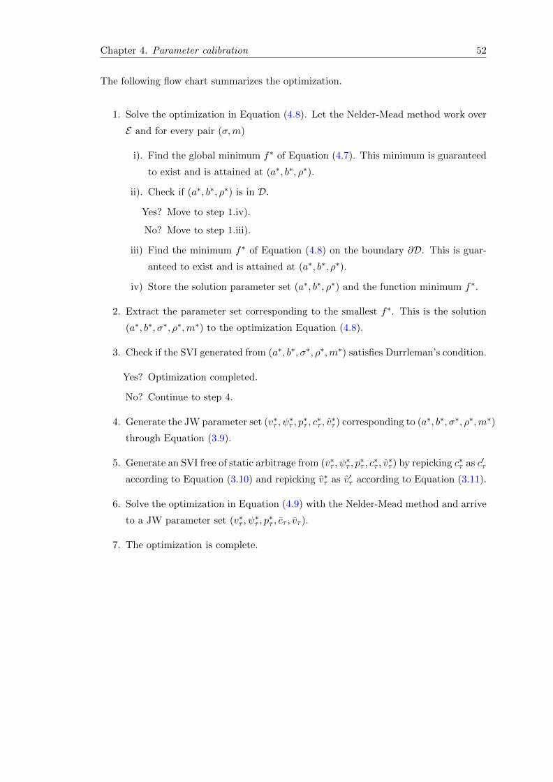
Chapter 4. Parameter calibration 52
The following flow chart summarizes the optimization.
1. Solve the optimization in Equation (4.8). Let the Nelder-Mead method work over
E and for every pair (σ,m)
i). Find the global minimum f∗ of Equation (4.7). This minimum is guaranteed
to exist and is attained at (a∗, b∗, ρ∗).
ii). Check if (a∗, b∗, ρ∗) is in D.
Yes? Move to step 1.iv).
No? Move to step 1.iii).
iii) Find the minimum f∗ of Equation (4.8) on the boundary ∂D. This is guar-
anteed to exist and is attained at (a∗, b∗, ρ∗).
iv) Store the solution parameter set (a∗, b∗, ρ∗) and the function minimum f∗.
2. Extract the parameter set corresponding to the smallest f∗. This is the solution
(a∗, b∗, σ∗, ρ∗,m∗) to the optimization Equation (4.8).
3. Check if the SVI generated from (a∗, b∗, σ∗, ρ∗,m∗) satisfies Durrleman’s condition.
Yes? Optimization completed.
No? Continue to step 4.
4. Generate the JW parameter set (v∗τ , ψ∗τ , p∗τ , c∗τ , v∗τ ) corresponding to (a∗, b∗, σ∗, ρ∗,m∗)
through Equation (3.9).
5. Generate an SVI free of static arbitrage from (v∗τ , ψ∗τ , p∗τ , c∗τ , v∗τ ) by repicking c∗τ as c′τ
according to Equation (3.10) and repicking v∗τ as v′τ according to Equation (3.11).
6. Solve the optimization in Equation (4.9) with the Nelder-Mead method and arrive
to a JW parameter set (v∗τ , ψ∗τ , p∗τ , cτ , vτ ).
7. The optimization is complete.

Chapter 5
Numerical experiments
5.1 The Vogt smile: the elimination of static arbitrage
The Vogt smile constitutes an example of an SVI parameter set that does not satisfy
Durrleman’s condition. The set is in the raw parameterization
(a, b, σ, ρ,m) = (−0.041, 0.1331, 0.4153, 0.306, 0.3586). (5.1)
The constraint in Equation (4.1) implies that the parameter set in Equation (5.1) could
never be an output from the calibration algorithm described in Chapter 4. It is however
possible to generate an implied volatility smile and its corresponding Durrleman’s con-
dition, and these are presented in Figure 5.1. The right plot illustrates the violation of
Durrleman’s condition; the graph is not everywhere non-negative.
−1.5 −1 −0.5 0 0.5 1 1.50
0.02
0.04
0.06
0.08
0.1
0.12
0.14
0.16
0.18
0.2
Moneyness
Impl
ied
vola
tility
−1.5 −1 −0.5 0 0.5 1 1.5−0.2
0
0.2
0.4
0.6
0.8
1
1.2
1.4
Moneyness
Dur
rlem
an’s
con
ditio
n
Figure 5.1: Left plot: The implied volatility corresponding to the parameters inEquation (5.1) is plotted against moneyness. Right plot: Durrleman’s condition corre-
sponding to the parameters in Equation (5.1) is plotted against moneyness.
53

Chapter 5. Numerical results 54
The time to maturity is needed to generate the JW parameters corresponding to the raw
parameters in Equation (5.1), but its value is not of importance and can be arbitrarily
chosen. For simplicity, and to follow Gatheral in [2] as close as possible, the time to
maturity is set to τ = 1. The JW parameters corresponding to the parameters in
Equation (5.1) are then
(vτ , ψτ , pτ , cτ , vτ ) = (0.0131,−0.1366, 0.7472, 1.5826, 0.0106). (5.2)
If vτ , ψτ , pτ are fixed and cτ , vτ are repicked according to Equation (3.10) and Equa-
tion (3.11), the new set of JW parameters gives a volatility smile that is guaranteed to
be free of butterfly arbitrage. The new parameter values are
c′τ = pτ + 2ψτ = 0.4740,
v′τ = vτ4pτ c
′τ
(pτ + c′τ )2 = 0.0124,
and the set of JW parameters that guarantees absence of butterfly arbitrage is thus
(vτ , ψτ , pτ , c′τ , v′τ ) = (0.0131,−0.1366, 0.7472, 0.4740, 0.0124). (5.3)
The implied volatility and Durrleman’s condition corresponding to this set of parameters
is presented in Figure 5.2 together with the arbitrageable volatility from Figure 5.1.
−1.5 −1 −0.5 0 0.5 1 1.50
0.02
0.04
0.06
0.08
0.1
0.12
0.14
0.16
0.18
0.2
Moneyness
Impl
ied
vola
tility
−1.5 −1 −0.5 0 0.5 1 1.5−0.2
0
0.2
0.4
0.6
0.8
1
1.2
1.4
1.6
Moneyness
Dur
rlem
an’s
con
ditio
n
Figure 5.2: Solid lines correspond to the parameter set in Equation (5.3) and dashedlines correspond to the parameter set in Equation (5.1). Left plot: Implied volatilitycorresponding to the parameter sets is plotted against moneyness. Right plot: Durrle-
man’s condition corresponding to the parameter sets is plotted against moneyness.
In the left plot of Figure 5.2, the effect of repicking cτ is observable. Since the value of
cτ was lowered to about a thrid of its original value, the slope of the right wing of the
smile is flatter. The right plot confirms that the SVI corresponding to the parameters

Chapter 5. Numerical results 55
in Equation (5.3) do satisfy Durrleman’s condition, since the green solid line is positive
everywhere.
Recall the discussion in Chapter 4 leading to the optimization in Equation (4.9). The
JW parameterization is continuous in all its parameters. Therefore, there exists a JW
parameterization (vτ , ψτ , pτ , c∗τ , v∗τ ) between the one in Equation (5.2) and the one in
Equation (5.3) that satisfies Durrleman’s condition and is as close as possible, in some
sense, to (vτ , ψτ , pτ , c′τ , v′τ ). This parameterization is found by optimizing (cτ , vτ ) over
the set [0.4740, 1.5826]× [0.0106, 0.0124] according to Equation (4.9). The Nelder-Mead
method was used as optimization algorithm. The optimal result was found to be
c∗τ = 1.3743,
v∗τ = 0.0110,
and is illustrated in Figure 5.3.
−1.5 −1 −0.5 0 0.5 1 1.50
0.02
0.04
0.06
0.08
0.1
0.12
0.14
0.16
0.18
0.2
Moneyness
Impl
ied
vola
tility
−1.5 −1 −0.5 0 0.5 1 1.5−0.2
0
0.2
0.4
0.6
0.8
1
1.2
1.4
1.6
Moneyness
Dur
rlem
an’s
con
ditio
n
Figure 5.3: The solid lines correspond to the, according to Equation (4.9), optimal setof JW parameters, the dashed red lines that lie on top of the solid lines correspond to theoriginal parameter set in Equation (5.1) and the deviant green dashed lines correspondto the parameter set in Equation (5.3). Left plot: Implied volatility corresponding tothe parameter sets is plotted against moneyness. Right plot: Durrleman’s condition
corresponding to the parameter sets is plotted against moneyness.

Chapter 5. Numerical results 56
5.2 Calibration to market data: the weighting of options
In this section, the SVI model will be fitted to raw market data. Before the calibration
method is applicable, the market data has to be prepared. This preperation is treated
in Section 5.2.1. One set of data on European put and call options written on the S&P
500 index, commonly refered to as SPX options. The S&P 500 index was discussed in
Chapter 2.1.
5.2.1 Data preperation
The market data used consists of a set of strikes and for each strike, bid and ask prices
for European call and put options written on that strike together with their corre-
sponding traded volume. Also, the price of the underlying and the time to maturity is
given. All prices are quoted in USD. Without loss of generality, let the current time be 0.
To apply the calibration, the forward price of the underlying and the interest rate of the
market need to be known. The forward price of the underlying can be derived from the
Put-Call parity,
C(τ,K)− P (τ,K) = S0 − e−rτK. (5.4)
The forward price of the underlying, F[0,τ ] = S0erτ , is hence equal to the strike at which
the call put and the put price are equal. This may happen in between data points. In
that case the strike where the prices agree is found by a linear interpolation between
the nearest data points. Note that since we now know the price of the underlying and
the forward price of the underlying for some expiry time we also know the interest rate
from today, t = 0, until that time.
All variables that are needed in the calibration are now at hand. It is time to look
at the quality of the information each data point carries. The quality, and therefore
importance, of the information of a data point will be judged by the trading volume of
that option. If there are options on the market without volume, illiquid options, then
these are removed from the data set. The illiquid options provide us with prices at
which nobody is trading and therefore they carry no information about the real price of
the option. In the next step, call options that have a strike price lower than the market
price of the underlying and put options with a strike price that is higher than the mar-
ket price of the underlying are discarded. Those that are kept, the out-of-the-money
options, tend to be more precise in pricing since they are bearing higher risk than the
ones we discarded, the in-the-money options. The out-of-the-money put option prices
are then translated into in-the-money call option prices via Equation (5.4) to create a
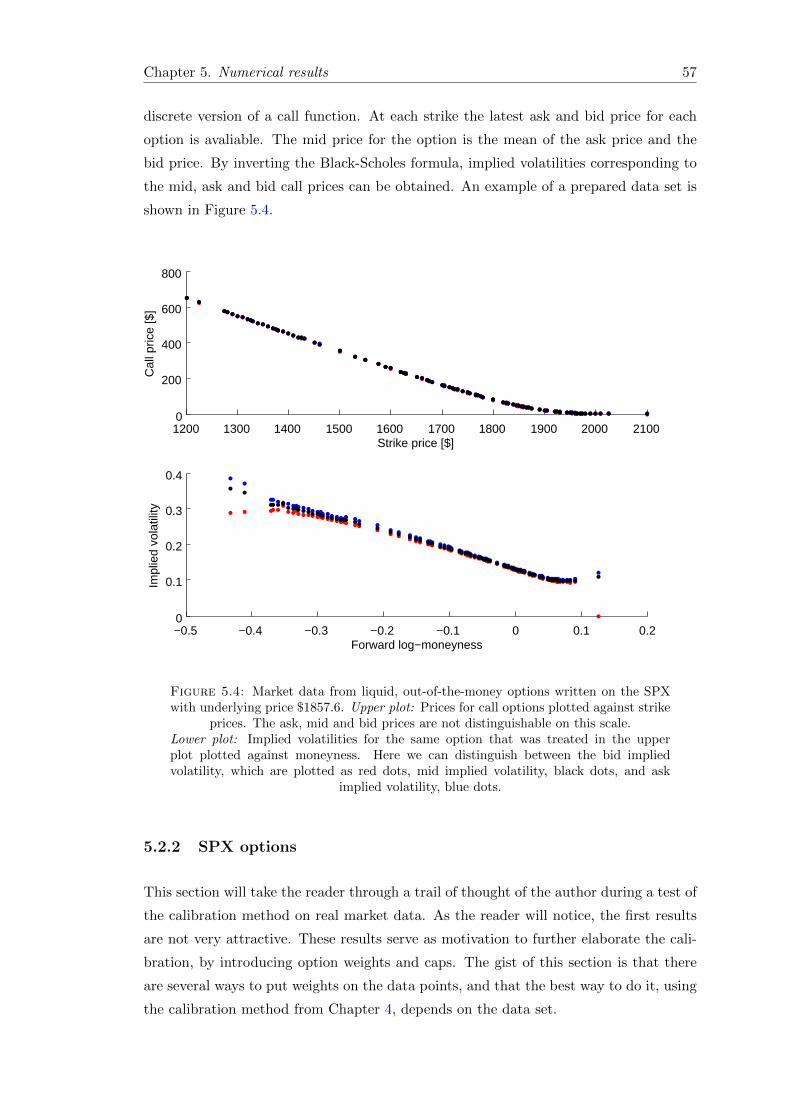
Chapter 5. Numerical results 57
discrete version of a call function. At each strike the latest ask and bid price for each
option is avaliable. The mid price for the option is the mean of the ask price and the
bid price. By inverting the Black-Scholes formula, implied volatilities corresponding to
the mid, ask and bid call prices can be obtained. An example of a prepared data set is
shown in Figure 5.4.
1200 1300 1400 1500 1600 1700 1800 1900 2000 21000
200
400
600
800
Strike price [$]
Cal
l pric
e [$
]
−0.5 −0.4 −0.3 −0.2 −0.1 0 0.1 0.20
0.1
0.2
0.3
0.4
Forward log−moneyness
Impl
ied
vola
tility
Figure 5.4: Market data from liquid, out-of-the-money options written on the SPXwith underlying price $1857.6. Upper plot: Prices for call options plotted against strike
prices. The ask, mid and bid prices are not distinguishable on this scale.Lower plot: Implied volatilities for the same option that was treated in the upperplot plotted against moneyness. Here we can distinguish between the bid impliedvolatility, which are plotted as red dots, mid implied volatility, black dots, and ask
implied volatility, blue dots.
5.2.2 SPX options
This section will take the reader through a trail of thought of the author during a test of
the calibration method on real market data. As the reader will notice, the first results
are not very attractive. These results serve as motivation to further elaborate the cali-
bration, by introducing option weights and caps. The gist of this section is that there
are several ways to put weights on the data points, and that the best way to do it, using
the calibration method from Chapter 4, depends on the data set.

Chapter 5. Numerical results 58
The first choice that is faced is what implied volatility data to use in the calibration.
Ask, bid and mid implied volatility data is avaliable, but all values in the interval be-
tween the bid and the ask, called the bid-ask spread, are feasible. The SVI in this
calibration are calibrated to mid implied volatility. In Figure 5.5, the SVI fit together
with bid (smaller) and ask (larger) implied volatilites are presented. Only every third
ask and bid implied volatility is plotted, so that it is possible to distinguish between
data point in the graphs.
−0.6 −0.4 −0.2 0 0.20
0.1
0.2
0.3
0.4
0.5
0.6
0.7Time to maturity = 0.096 years
Forward log−moneyness
Vol
atili
ty
−0.5 −0.4 −0.3 −0.2 −0.1 0 0.1 0.20
0.05
0.1
0.15
0.2
0.25
0.3
0.35
0.4
0.45
0.5Time to maturity = 0.137 years
Forward log−moneyness
Vol
atili
ty
−0.5 −0.4 −0.3 −0.2 −0.1 0 0.1 0.20.05
0.1
0.15
0.2
0.25
0.3
0.35
0.4
0.45Time to maturity = 0.175 years
Forward log−moneyness
Vol
atili
ty
−1 −0.8 −0.6 −0.4 −0.2 0 0.2 0.40
0.1
0.2
0.3
0.4
0.5
0.6
0.7Time to maturity = 0.233 years
Forward log−moneyness
Vol
atili
ty
Figure 5.5: Implied volatility plotted against moneyness for four different times tomaturity. The red dots are bid implied volatility, the blue line is the SVI fit to midimplied volatility and the black dots are ask implied volatility. Only every third ask
and bid implied volatility is plotted.
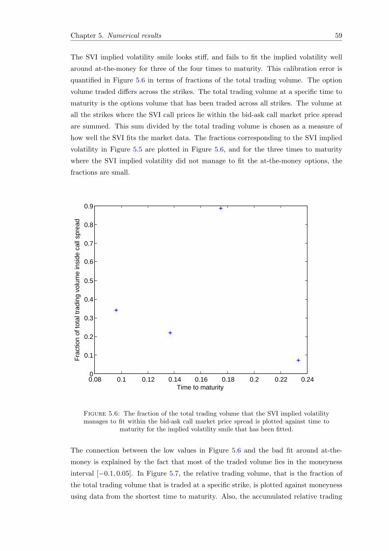
Chapter 5. Numerical results 59
The SVI implied volatility smile looks stiff, and fails to fit the implied volatility well
around at-the-money for three of the four times to maturity. This calibration error is
quantified in Figure 5.6 in terms of fractions of the total trading volume. The option
volume traded differs across the strikes. The total trading volume at a specific time to
maturity is the options volume that has been traded across all strikes. The volume at
all the strikes where the SVI call prices lie within the bid-ask call market price spread
are summed. This sum divided by the total trading volume is chosen as a measure of
how well the SVI fits the market data. The fractions corresponding to the SVI implied
volatility in Figure 5.5 are plotted in Figure 5.6, and for the three times to maturity
where the SVI implied volatility did not manage to fit the at-the-money options, the
fractions are small.
0.08 0.1 0.12 0.14 0.16 0.18 0.2 0.22 0.240
0.1
0.2
0.3
0.4
0.5
0.6
0.7
0.8
0.9
Fra
ctio
n of
tota
l tra
ding
vol
ume
insi
de c
all s
prea
d
Time to maturity
Figure 5.6: The fraction of the total trading volume that the SVI implied volatilitymanages to fit within the bid-ask call market price spread is plotted against time to
maturity for the implied volatility smile that has been fitted.
The connection between the low values in Figure 5.6 and the bad fit around at-the-
money is explained by the fact that most of the traded volume lies in the moneyness
interval [−0.1, 0.05]. In Figure 5.7, the relative trading volume, that is the fraction of
the total trading volume that is traded at a specific strike, is plotted against moneyness
using data from the shortest time to maturity. Also, the accumulated relative trading

Chapter 5. Numerical results 60
volume, that is all the volume traded at all strikes smaller or equal to a specific strike,
is plotted against moneyness. The concentration of volume is clearly visible in the steep
ascent of the thick red line, about 80% of the trading volume was lying in the moneyness
interval [−0.1, 0.05].
−0.6 −0.5 −0.4 −0.3 −0.2 −0.1 0 0.1 0.20
0.02
0.04
0.06
0.08
0.1
0.12
0.14
Forward log−moneyness
Rel
ativ
e tr
adin
g vo
lum
e
Time to maturity = 0.096 years
−0.6 −0.5 −0.4 −0.3 −0.2 −0.1 0 0.1 0.20
0.1
0.2
0.3
0.4
0.5
0.6
0.7
0.8
0.9
1
Acc
umul
ated
rel
ativ
e tr
adin
g vo
lum
e
Figure 5.7: The concentration of trading volume around the origin.Left axis: The relative trading volume, blue dots, is plotted against moneyness.
Right axis: The accumulated relative trading volume, red line, is plotted against mon-eyness.
The importance of the high volume options is not considered in the calibration method
of Chapter 4 where all options were treated equally. Introducing weights on the options
in the objective functions of the optimization reflecting their importance comes to mind
as a natural solution to this. Therefore Equation (4.8) is replaced with the optimization
min(σ,m)∈E
n∑i=1
Wi
(w(a∗,b∗,σ,ρ∗,m) − wi
)2, (5.5)
where W1, . . . ,Wn are the weights. What weights to use is a choice of the implementor.
The relative trading volume of the options, or some increasing function of it, is a strong
candidate. The relative trading volume reflects each individual option’s fraction of the
total market volume. Another candidate is the vega of the option, or some increasing
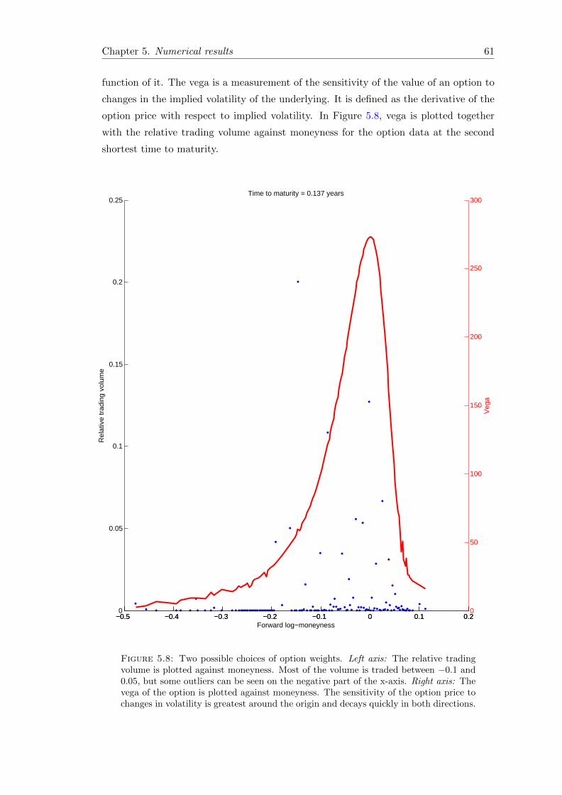
Chapter 5. Numerical results 61
function of it. The vega is a measurement of the sensitivity of the value of an option to
changes in the implied volatility of the underlying. It is defined as the derivative of the
option price with respect to implied volatility. In Figure 5.8, vega is plotted together
with the relative trading volume against moneyness for the option data at the second
shortest time to maturity.
−0.5 −0.4 −0.3 −0.2 −0.1 0 0.1 0.20
0.05
0.1
0.15
0.2
0.25
Forward log−moneyness
Rel
ativ
e tr
adin
g vo
lum
e
Time to maturity = 0.137 years
−0.5 −0.4 −0.3 −0.2 −0.1 0 0.1 0.20
50
100
150
200
250
300
Veg
a
Figure 5.8: Two possible choices of option weights. Left axis: The relative tradingvolume is plotted against moneyness. Most of the volume is traded between −0.1 and0.05, but some outliers can be seen on the negative part of the x-axis. Right axis: Thevega of the option is plotted against moneyness. The sensitivity of the option price tochanges in volatility is greatest around the origin and decays quickly in both directions.

Chapter 5. Numerical results 62
The shape of the vega in Figure 5.8 is characteristic for the vega of a call option, hence
prices of call options are not sensitive to large changes in volatility at strikes far from
at-the-money. This implies that if the same volume is traded at some strike far from at-
the-money and at some strike at-the-money, it is more important to fit the at-the-money
option well. In this calibration the weights were chosen to be the product between the
relative trading volume and the vega,
Wi = Relative trading volume at strike number i×Vega at strike number i. (5.6)
One more question needs to be settled. Since the SVI only has five parameters, it will
never be able to fit the mid implied volatility for all options. If fewer options are used
in the fit, the SVI will be able to fit these options better. Assume that the N heaviest
options are used in the calibration. How does the SVI overall performance depend on
N? Does the SVI nessecarily do better just because we calibrate it to more data points?
In Figure 5.9, the fraction of the total trading volume that the SVI fitted inside the call
spread is plotted against N , the number of options in heavy to light order, used in the
calibration.
0 50 100 1500.1
0.2
0.3
0.4
0.5
0.6
0.7
0.8
0.9
1
Number of options in fit
Fra
ctio
n of
tota
l tra
ding
vol
ume
insi
de c
all s
prea
d
Time to maturity = 0.096
0 50 100 1500.1
0.2
0.3
0.4
0.5
0.6
0.7
0.8
0.9
1
Number of options in fit
Fra
ctio
n of
tota
l tra
ding
vol
ume
insi
de c
all s
prea
d
Time to maturity = 0.137
0 20 40 60 80 1000.1
0.2
0.3
0.4
0.5
0.6
0.7
0.8
0.9
1
Number of options in fit
Fra
ctio
n of
tota
l tra
ding
vol
ume
insi
de s
prea
d
Time to maturity = 0.175
0 20 40 60 80 1000
0.1
0.2
0.3
0.4
0.5
0.6
0.7
0.8
0.9
1
Number of options in fit
Fra
ctio
n of
tota
l tra
ding
vol
ume
insi
de c
all s
prea
d
Time to maturity = 0.233
Figure 5.9: The fraction of the market which was fitted inside the call spread as afunction of the number of options used in the calibration.

Chapter 5. Numerical results 63
For three of the maturities, the general pattern is that the overall performance becomes
better and better the more options we use. The top right corner plot breaks this pattern,
and the shape of that plot is sometimes seen in market data. In the light of the plots in
Figure 5.9 we chose to calibrate the SVI after the Nmax heaviest options, where Nmax is
the number where the graphs in Figure 5.9 reach their maximum. To summarize,
• all options are weighted according to Equation (5.6),
• the options are ordered according to their weights,
• the Nmax heaviest options are used in the calibration, where Nmax is the number
at which the experiment illustrated in Figure 5.9 attains its maximum.
The result of this new calibration is presented in Figure 5.10. Compared to the fits in
Figure 5.5, the new calibration looks better. By looking at the fraction of total trading
volume that the new calibration fit inside the bid-ask call price spread, this is confirmed.
The fractions are presented in Figure 5.11. The fit is still not perfect for short times to
maturity, but this is expected. Short lived options are generally much more difficult to fit.
Figure 5.11 shows that still not all the volume is hit by the SVI. It is interesting to
know which options that were fitted outside the bid-ask spread and how far away from
the spread these misfitted prices are. Where are the thieves lurking that the SVI misses,
and how dangerous are they? This question is answered by Figure 5.12. Only for the
shortest time to maturity does the SVI miss the bid-ask spread close to the at-the-money.
Otherwise, the misses are far out-of-the-money.
Finally, no butterfly arbitrage was detected for the SVI implied volatilitiy in Figure 5.10.
This was an expected result, since the SPX is one of the most liquid options on the mar-
ket. In Figure 5.13, Durrleman’s condition corresponding to the SVI fits is plotted. Is
is everywhere positive, which implies absence of butterfly arbitrage.
We have now seen the calibration method in action. It is able to eliminate static arbi-
trage from an implied volatility smile given by a set of SVI parameters and it manages
to produce good fits to real market data. Thus this research has generated a calibration
model that fulfills the purpose of this thesis within the stated delimitations. We let the
following plots conclude this chapter and the thesis.

Bibliography 64
−0.6 −0.4 −0.2 0 0.20
0.1
0.2
0.3
0.4
0.5
0.6
0.7Time to maturity = 0.096
Forward log−moneyness
Impl
ied
Vol
atili
ty
−0.6 −0.4 −0.2 0 0.20
0.05
0.1
0.15
0.2
0.25
0.3
0.35
0.4
0.45
0.5Time to maturity = 0.137
Forward log−moneyness
Impl
ied
Vol
atili
ty
−0.6 −0.4 −0.2 0 0.20.05
0.1
0.15
0.2
0.25
0.3
0.35
0.4
0.45Time to maturity = 0.175
Forward log−moneyness
Impl
ied
Vol
atili
ty
−1 −0.5 0 0.50
0.1
0.2
0.3
0.4
0.5
0.6
0.7Time to maturity = 0.233
Forward log−moneyness
Impl
ied
Vol
atili
ty
Figure 5.10: New SVI implied volatility fit using weights and caps in the calibration.The red dots are bid implied volatility, the blue line is the SVI fit to mid impliedvolatility and the black dots are ask implied volatility. Only every third ask and bid
implied volatility is plotted.

Bibliography 65
0.08 0.1 0.12 0.14 0.16 0.18 0.2 0.22 0.240.92
0.93
0.94
0.95
0.96
0.97
0.98
0.99
1
Time to maturity
Fra
ctio
n of
tota
l tra
ding
vol
ume
insi
de c
all s
prea
d
Figure 5.11: The fraction of the total trading volume that the new SVI impliedvolatility, calibrated with weights and caps, manages to fit within the bid-ask call pricespread is plotted against time to maturity for the implied volatility smile that has been
fitted.
1000 1500 2000 25000
0.1
0.2
0.3
0.4
Strike price [$]
Dis
tanc
e fr
om s
prea
d [$
]
Time to maturity = 0.096
1000 1500 2000 25000
0.1
0.2
0.3
0.4
Strike price [$]
Dis
tanc
e fr
om s
prea
d [$
]
Time to maturity = 0.137
1000 1500 2000 25000
0.1
0.2
0.3
0.4
Strike price [$]
Dis
tanc
e fr
om s
prea
d [$
]
Time to maturity = 0.175
500 1000 1500 2000 25000
0.1
0.2
0.3
0.4
Strike price [$]
Dis
tanc
e fr
om s
prea
d [$
]
Time to maturity = 0.233
Figure 5.12: The amount that the SVI generated call prices miss the bid-ask callprice spread at each strike plotted for the four times to maturity.

Bibliography 66
−0.6 −0.4 −0.2 0 0.20
0.5
1
1.5
2Time to maturity = 0.096 years
Forward log−moneyness
Dur
rlem
an’s
con
ditio
n
−0.2 −0.1 0 0.1 0.20
0.5
1
1.5
2Time to maturity = 0.137 years
Forward log−moneyness
Dur
rlem
an’s
con
ditio
n
−0.6 −0.4 −0.2 0 0.20
0.5
1
1.5
2Time to maturity = 0.175 years
Forward log−moneyness
Dur
rlem
an’s
con
ditio
n
−0.6 −0.4 −0.2 0 0.20
1
2
3Time to maturity = 0.233 years
Forward log−moneyness
Dur
rlem
an’s
con
ditio
n
Figure 5.13: Durrleman’s condition plotted corresponding to the new SVI impliedvolatility for the four times to maturity.

Bibliography
[1] Gatheral, J. A parsimonious arbitrage-free implied volatility parameterization with
application to the valuation of volatility derivatives. Presentation at Global Deriva-
tives & Risk Management, Madrid, 2004.
[2] Gatheral, J.,Jacquier, A. Arbitrage-free SVI volatility surfaces. Quantitative Fi-
nance, 14(1):59–71, 2014.
[3] Wilmott, P. Paul Wilmott on Quantitative Finance. John Wiley & Sons, 2000.
[4] Gatheral, J. The Volatility Surface: A Practitioner’s Guide. Wiley Finance, 2006.
[5] Madan, D.B., Yor, M. Making Markov martingales meet marginals: with explicit
constructions. Bernoulli, 8(4):509–536, 2002.
[6] Carr, P., Geman, H., Madan, D.B., Yor, M. Stochastic volatility for Levy processes.
Mathematical Finance, 13(3):345–382, July 2003.
[7] Kellerer, H.G. Markov-Komposition und eine Anwendung auf Martingale. Mathe-
matische Annalen, 198(3):99–122, 1972.
[8] Durrett, R. Probability, Theory and Examples. Cambridge University Press, 2010.
[9] Hirsch, F., Roynette, B. A new proof of Kellerer’s theorem. ESAIM: Probability
and Statistics, 16:48–60, 2012.
[10] Hirsch, F., Roynette, B., Yor, M. Kellerer’s theorem revisited. Unpublished, 2012.
[11] Follmer, H., Schied, A. Stochastic Finance: An Introduction in Discrete Time, 2nd
ed. Walter de Gruyter GmbH & Co, 2004.
[12] Rooper, M. Arbitrage Free Implied Volatility Surfaces. Preprint; avaliable at
http://www.maths.usyd.edu.au/u/pubs/publist/preprints/2010/roper-9.pdf.
[13] Hirsch, F., Profeta, C., Roynette, B., Yor, M. Peacocks and Associated Martingales,
with Explicit Constructions. Springer Milan, 2011.
[14] Lowther, G. Limits of one-dimensional diffusions. 37:78–106, 2009.
67

Bibliography 68
[15] Durrleman, V. A note on initial volatility surface. Unpublished, February 2003.
[16] Fengler, R. Arbitrage-Free Smoothing of the Implied Volatility Surface. Quantita-
tive Finance, 9(4):417–428, 2009.
[17] Broadie, M., Cvitanic, J., Soner, H.M. Optimal Replication of Contingent Claims
under Portfolio Constraints. The Review of Financial Studies, 11(1):59–79, 1998.
[18] Lee, R. The moment formula for implied volatility at extreme strikes. Mathematical
Finance, 14(3):469–480, 2004.
[19] Benaim, S., Friz, P., Lee, R. On Black-Scholes Implied Volatility at Extreme Strikes.
Frontiers in Qualitative Finance: Volatility and Credit Risk Modeling, 2008.
[20] Hagan, P.S.,Kumar, D.,Lesniewski, A.S.,Woodward, D.E. Managing Smile Risk.
Wilmott Magazine, 1:84–108, 2002.
[21] Damghani, B.M., Kos, A. De-arbitraging With a Weak Smile: Application to Skew
Risk. Wilmott, (64):40–49, 2013.
[22] Hodges, S., Zhao, B. Parametric modeling of implied smile functions: a generalized
SVI model. Review of Derivatives Research, 16:53–77, april 2013.
[23] Gatheral, J., Jacquier, A. Convergence of Heston to SVI. Quantitative Finance, 11
(8):1129–1132, 2011.
[24] Castagno, A.,Mercurio, F. The vanna-volga method for implied volatilities. Risk
Magazine, 20(1):106–111.
[25] Guo, G., Jacquier, A., Martini, C., Neufcourt, L. Generalised arbitrage-free SVI
volatility surfaces. Preprint at arXiv:1210.7111, 2013.
[26] Zeliade Systems. Quasi-explicit calibration of Gatheral’s SVI model. Zeliade White
Papers, 2009.
[27] De Marco, S. On Probability Distributions of Diffusions and Financial Models with
non-globally smooth coefficients. Ph.D. thesis at Universite Paris-Est, November
2010.
[28] Rogers, L.C.G. Tehranchi, M.R. Can the implied volatility surface move by parallel
shifts? Finance and Stochastics, 14(2):235, 2010.
[29] Leursen, M.A., Le Riche, R. Globalized Nelder-Mead method for engineering opti-
mization. Computers & Structures, 82(23-26):2251–2260, 2004.
[30] Carr, P., Madan, D.B. Towards a Theory of Volatility Trading. Volatility, risk
publications, Jarrow, R., 1998.

Appendix A
Nelder-Mead method
The Nelder-Mead method is a simplex method for finding a local minimum of a function
of several variables. It employs a pattern search, which will be described below, that
compares function values at the vertices of the simplex. The objective function is evalu-
ated at all vertices. The worst vertex, that is the vertex that gives the highes objective
function value, is rejected and replaced by a new vertex. A new simplex is formed and a
new comparison is made. After itterating this algorithm, the simplices will zoom in on
a local minium and will have decreased in size so that eventually, they approximate the
local minimum. By rerunning the algorithm from various initial points, all local minima
can be found and hence also the global minimum.
Probabilistic restarts
Local optimizers can make up a global search when repeatedly started from different
initial points. In the SVI calibration, the Nelder Mead method is applied to a non-linear
function that can have multiple minima. Therefore, a global search is necessary. In [29],
the authors introduce a method to choose the initial points. Their procedure involve a
random sampling of a set of points, and then a selection of the initial point from this set
by measuring the distance, in some sense, to the previous initial points. This procedure
saves us from the task of defining a grid of initial points, which would have been the
case in a deterministic search. Thus we do not have to know how many times we have
to restart the algorithm in advance. The procedure also uses information about past
searches, which a pure random choice of initial points would not. Thus the precedure
has a low chance of choosing a initail point close to some old initial point, and therefore
finding the same local minimum twice.
69

Appendix A. Nelder-Mead method 70
If we have already sampled a set xiNi=1 of initial points for the algorithms, let the
probability of sampling a point x ∈ Rn to be the initial point be
p(x) =1
N
N∑i=1
pi(x), (A.1)
where
pi(x) =1
(2π)n/2det(Σ)1/2e−
12
(x−xi)TΣ−1(x−xi). (A.2)
Here, n is the dimension of Rn, the space we run the optimize in, and Σ is the covariance
matrix. It is suggested in [29] to estimate the covariances, σ2j , by
σ2j = α(xmax
j − xminj )2, j = 1, . . . , n,
where α is a positive parameter that controls the width of the Gaussian bell in Equa-
tion (A.2) and xmaxj and xmin
j are the upper and lower bounds for the feasible region in
the j:th direction. A value for α that works will with the SVI implementation is 0.1.
By casting points randomly from a uniform distribution on the feasible set, we get
candidates to the initial point for the algorithm. We can then order these candidates by
evaluating (A.1) at all the casted points. The point which generates the smallest value
of Equation (A.1), the point which has the least probability of being casted given earlier
initail points, is selected as initial point.
The algorithm, step by step
Let s0 be the initial simplex with vertices x1, . . . , xn. Let f be the objective function we
want to minimize.
i) Reorder the vertices with respect to their objective function values, that is if
f(x1) ≤ · · · ≤ f(xn)
then x1 is the best point and xn is the worst point.
ii) Calculate the center of mass of s0\xn, the initial simplex without the worst point,
xc =1
n− 1
n−1∑i=1
xi

Appendix A. Nelder-Mead method 71
iii) Calculate the reflection, xr of the worst point, xn with respect to xm,
xr = xm + ρ(xm − xn).
The choice of ρ does not necessarly have to be 1, but has to be positive. If xr is
better that the second worst point xn, but not better than the best point x1, that
is
f(x1) ≤ f(xr) ≤ f(xn − 1),
then let the new simplex s1 be s0 but with the worst point xn replaced by xr. In
this case, restart the algorithm from step i). Otherwise, move on to step iv).
iv) If xr is better than the best point x1, that is f(xr) < f(x1), then calculate the
expansion xe of xn with respect to xm,
xe = xm + η(xm − xn), η > ρ.
If xe is better than xr, that is f(xe) < f(xr), then let the new simplex be s0 but
with the worst point xn replaced by xe and restart the algorithm from step i). If
that is not the case, then the new simplex is s0 with the worst point xn replaced
by xr.
v) Now f(xr) ≥ f(xn−1), so calculate the contraction xc of xn through xm,
xc = xm − c(xm − xn), 0 < c < ρ.
If xc is better than the worst point, that is f(xc) < f(xn), then let the new simplex
be s0 but with the worst point xn replaced by xc and restart the algorithm from
step i). If that is not the case, go to step vi).
vi) Replace all vertices except the best one, xini=2, with their contractions towards
the best one, x′ini=2,
x′i = x1 + σ(xi − x1).
Now let the new simplex be the convex hull of x1 ∪ x′ini=2 and return to step
i).
Figure A.1 illustrates one iteration of the algorithm.

Appendix A. Nelder-Mead method 72
Figure A.1: One iteration of the Nelder-Mead algorithm with ρ = 1, η = 2, c = 1/2and σ = 1/3.
Appendix B
Spanning a payoff with bonds and
options
The following spanning formula was derived in [30] by Carr and Madan.
Using Dirac’s delta function, we can for any function f(s) write for some k ≥ 0.
f(s) =
∫ ∞0
f(K)δ(s−K)dK
=
∫ k
0f(K)δ(s−K)dK +
∫ ∞k
f(K)δ(s−K)dK,
Recall that
∫ b
aδ(s−K)d = H(s < K)|ba, where H is the Heaviside function. Integrating
the previous equation by parts gives
f(s) = f(K)H(s < K)|k0 −∫ k
0f ′(K)H(s < K)dK
+ f(K)H(s ≥ K)|∞k +
∫ ∞k
f ′(K)H(s ≥ K)dK.
Integrating the integrals by parts one more time yields,
f(s) = f(K)H(s < K)|k0 + f ′(K)(K − s)+∣∣k0
+
∫ k
0f ′′(K)(K − s)+dK
+ f(K)H(s ≥ K)|∞k + f ′(K)(s−K)+∣∣∞k
+
∫ ∞k
f ′′(K)(s−K)+dK.
Making the economic interpretation of f(s) as a payoff on a contract written on an
underlying s, and K as the strike, we can impose the boundary condition f(0) = 0. Any
73

Appendix B. Spanning a payoff with bonds and options 74
other payoff at 0 would create arbitrage. Then the last equation becomes
f(s) = f(k) + f ′(k)((s− k)+ − (k − s)+
)+
∫ k
0f ′′(K)(K − s)+dK +
∫ ∞k
f ′′(K)(s−K)+dK.

Appendix C
Call price derivative
Using the notation from Chapter 2.4, this appendix presents the calculations behind all
used derivatives of the Black-Scholes call price function.
Since we assume that implied volatility is non-constant over strikes, we have to be careful
when calculating the derivative of the call price with respect to strike. All dependencies
and subscripts will be dropped in the calculations that follow to avoid messyness, so lets
de a review of the dependencies of all involved functions,
CB : (τ,K, τσ2imp;F, r, t) 7→ F[t,t+τ ]N (d1)−KN (d2),
d1 : (τ,K, τσ2imp;F, r, t) 7→ − x
θimp+θimp
2,
d2 : (τ,K, τσ2imp;F, r, t) 7→ − x
θimp+θimp
2,
x : (F,K; t, τ) 7→ log(K/F[t,t+τ ]),
F : (t, τ ;S, r) 7→ Sterτ ,
σimp : (τ,K) 7→ σimp(τ,K),
θimp : (τ,K) 7→√τσimp(τ,K),
wimp : (τ,K) 7→ θ2imp(τ,K),
N : d 7→ 1√2π
∫ d
−∞e−t
2/2dt,
n : d 7→ 1√2πe−d
2/2.
All first and second order partial derivatives of CB with respect to moneyness and
implied volatility will be needed in the differentiation, so first these will be calculated
75

Appendix C. Call price derivatives 76
explicitly. A useful trick in the differentiation is the following,
n (d1) =1√2πe−
(x/θimp)2−x+(θimp/2)2
2
=ex√2πe−
(x/θimp)2+x+(θimp/2)2
2
= exn (d2) .
Lets calculate the partial derivatives.
∂xCB = F
(n(d1)∂xd1 − exN (d2)− exn(d2)∂xd2
)= F
(n(d1)
(− 1
θimp
)− exN (d2)− exn(d2)
(− 1
θimp
))= −FexN (d2).
∂σimpCB = F
(n(d1)∂θimp
(d1)∂σimp(θimp)− exn(d2)∂θimp(d2)∂σimp(θimp)
)= Fn(d1)
√τ
(x
θ2imp
+1
2− x
θ2imp
+1
2
)= Fn(d1)
√τ .
∂xxCB = −FexN (d2)− Fexn(d2)∂xx(d2)
= F
(−exN (d2) + n(d1)
(1
θimp
)).
∂xσimpCB = −Fexn(d2)∂σimp(d2)
= Fn(d1)√τ
(− x
θ2imp
+1
2
).
∂σimpσimpCB = F
√τ∂d1
(n(d1)
)∂σimp(d1)
= F√τn(d1)(−d1)
√τ
(x
θ2imp
+1
2
)
= Fn(d1)τ
(x
θimp− θimp
2
)(x
θ2imp
+1
2
)
= Fn(d1)τ
(x2
θ3imp
− θimp
4
).

Appendix C. Call price derivatives 77
Using the partial derivatives from above together with the chain rule for differentiation
of multivariable functions, we can calculate the derivatives that we are interested in.
∂KKCB = ∂K
(∂x(CB)∂K(x) + ∂σimp
(CB)∂K (σimp)
)(C.1)
= ∂xx(CB) (∂K(x)
)2+ ∂xσimp
(CB)∂K(x)∂K (σimp) + ∂x
(CB)∂KK(x)
+ ∂σimp∂x
(CB)∂K (σimp) ∂K (x) + ∂σimpσimp
(CB) (∂K (σimp)
)2+ ∂σimp
(CB)∂KK (σimp)
=1
K2∂xx
(CB)
+1
K2∂xσimp
(CB)∂x (σimp)− 1
K2∂x(CB)
+1
K2∂σimpx
(CB)∂x (σimp) +
1
K2∂σimpσimp
(CB) (∂x (σimp)
)2+
1
K2∂σimp
(CB) (− ∂x (σimp) + ∂xx (σimp)
)=
1
K2
(∂xx
(CB)
+ 2∂x (σimp) ∂xσimp
(CB)
+(∂x (σimp)
)2∂σimpσimp
(CB)
− ∂x(CB)
+(− ∂x (σimp) + ∂xx (σimp)
)∂σimp
(CB))
=Fn(d1)
K2
(1
θimp+√τ
(1− 2x
θ2imp
)∂x (σimp)
+ τ
(x
θ3imp
− θimp
4
)(∂x (σimp)
)2+√τ(− ∂x (σimp) + ∂xx (σimp)
))
=Fn(d1)
K2θimp
((1−√τx
θimp∂x (σimp)
)2
− τθ2
imp
4
(∂x (σimp)
)2+√τθimp∂xx (σimp)
).
It is useful to translate this expression into derivatives with respect to total implied
variance.
∂KK(CB)
=Fn(d1)
K2θimp
((1−√τx
θimp∂x (σimp)
)2
− τθ2
imp
4
(∂x (σimp)
)2(C.2)
+√τθimp∂xx (σimp)
)=
Fn(d1)
K2θimp
((1− x
θimp∂x (θimp)
)2
−θ2
imp
4
(∂x (θimp)
)2+ θimp∂xx (θimp)
)
=Fn(d1)
K2√wimp
((1− x√wimp
1
2√wimp
∂x (wimp)
)2
− wimp
4
1
4wimp(∂x (wimp))2
+√wimp
(1
2√wimp
∂xx (wimp)− 1
4w3/2imp
(∂x (wimp)
)2))
=Fn(d1)
K2√wimp
((1− x
2wimp∂x (wimp)
)2
− 1
4
(1
wimp+
1
4
)(∂x (wimp)
)2+
1
2∂xx (wimp)
).

Appendix C. Call price derivatives 78
Furthermore, in the proof of Theorem 5, the derivative of
f(wimp) =F
KN (d1)−N (d2)
with respect to total implied variance is needed.
∂wimpf(wimp) =F
Kn(d1)∂wimp(d1)− n(d2)∂wimp(d2) (C.3)
=F
Kexn(d2)∂wimp
(− x√wimp
+
√wimp
2
)− n(d2)∂wimp
(− x√wimp
−√wimp
2
)= n(d2)
1
2√wimp