PIDE Working Papers 2007:34

The Taylor Rule and the Macroeconomic Performance in Pakistan

Wasim Shahid Malik Pakistan Institute of Development Economics, Islamabad

Ather Maqsood Ahmed Central Board of Revenue, Islamabad

PAKISTAN INSTITUTE OF DEVELOPMENT ECONOMICS ISLAMABAD

2

All rights reserved. No part of this publication may be reproduced, stored in a retrieval system or transmitted in any form or by any means—electronic, mechanical, photocopying, recording or otherwise—without prior permission of the author(s) and or the Pakistan Institute of Development Economics, P. O. Box 1091, Islamabad 44000.

© Pakistan Institute of Development Economics, 2007.

Pakistan Institute of Development Economics Islamabad, Pakistan E-mail: publications@pide.org.pk Website: http://www.pide.org.pk Fax: +92-51-9210886

Designed, composed, and finished at the Publications Division, PIDE.

C O N T E N T S

Page Abstract v

1. Introduction 1

2. Monetary Policy Rules 3

2.1. Instrument Rules 4

2.2. Targeting Rules 6

2.3. Characteristics of the Instrument Rules in Developing

Countries Perspective 7

3. Methodology 8

3.1. Estimation 8

3.2. Macroeconomic Performance 9

3.3. Loss Minimisation 10

4. Estimation Results 11

4.1. Estimating the Taylor Rule for Pakistan 11

4.2. Macroeconomic Performance according to the Taylor Rule 14

4.3. Finding Optimal Parameter Values for Pakistan 16

4.4. Loss Function and Comparison of Parameter Values 20

4.5. Constrained Numerical Optimisation 21

5. Conclusion 23

Appendices 24

References 27

List of Tables

Table 1. Actual and Rule-induced Short Interest Rate 13

Table 2. Different Regimes of Governors 14

Table 3. Simulation with the Taylor Rule and the Estimated Model 16

2

Page Table 4. Estimation of Long-run Real Interest Rate 17

Table 5. Simulation with the First Best Set of Parameter Values 18

Table 6. Simulation with the Second Best Set of Parameter Values 19

Table 7. Loss Associated with Different Parameter Values for the Rule 21

Table 8. Loss Minimisation Subject to Different Constraints 22

List of Figures

Figure 1. Actual and the Taylor Rule-induced Short Interest Rate 13

Figure 2. Actual and Taylor Rule-induced Short Interest Rate, Output Gap, and Inflation 24

Figure 3. Actual and First Best Rule-induced Short Interest Rate, Output Gap, and Inflation 25

Figure 4. Actual and Second Best Rule-induced Short Interest Rate, Output Gap, and Inflation 26

ABSTRACT

A widely agreed proposition in modern economics is that policy rules have greater advantage over discretion in improving economic performance. Simple monetary policy instrument rules are feasible options for developing countries lacking the pre-requisites for more sophisticated targeting rules. Notwithstanding the focus of modern literature on the issue, the State Bank of Pakistan (SBP) has never declared itself to be following any type of rule. Surprisingly, this topic has remained out of research focus (among the academia and the practitioners) in Pakistan. This is the first attempt to deal with a rule-based monetary policy strategy in the case of the SBP. We have estimated the Taylor rule and simulated the economy using this rule as a monetary policy strategy. Our results indicate that the SBP has not been following the Taylor rule. In fact, the actual policy can be taken as an extreme deviation from it. On the other hand, counterfactual simulation confirms that macroeconomic performance can be improved, in terms of stability in inflation and output, when a simple Taylor rule is adopted. In this regard the parameter values (especially the inflation target) in the rule must be set according to the conditions of the economy under consideration rather than by relying on the ones suggested by the Taylor rule.

JEL classification: E47, E31, E52 Keywords: Taylor Rule, Macroeconomic Performance, Counterfactual

Simulation

1. INTRODUCTION*

The most agreed upon proposition in the modern macroeconomics is that policy rules have greater advantage over discretion in improving economic performance, [Taylor (1993)]. Kydland and Prescott (1977) and Barro and Gordon (1983) have convincingly put forward that discretionary policies are time inconsistent. Specifically stating, low inflationary policy becomes dynamically inconsistent in the presence of discretionary powers to monetary authority with the economic agents having rational expectations. Barro and Gordon (1983a) highlighted that punishment by private agents to the policy maker in case of acting against the announced rule, and the reputation problem faced by the monetary authority are solutions to the time inconsistency problem. Regarding this issue, Rogoff (1985) has suggested delegation of powers to conservative central banker who is known to be inflation averse. Similarly, Walsh (1995) established that punishment criterion set in the central banker’s contract could be a possible solution to the time inconsistency problem.

Whereas all this research confirms that rules are superior to discretion but it offers no clue as to how the rules could be used in practical policy making process. Taylor has resolved this issue in 1993, who offered a rule that is both practicable and simple. It suggests setting the short interest rate (monetary policy instrument) based on the state of the economy. Precisely, it calls for changes in the interest rate in response to deviation of output from trend or potential level and that of inflation from the target with equal weight given to both objectives in the policy reaction function. In this way policy maker would be able to solve the time inconsistency problem of optimal policies and this simple rule has the potential to improve macroeconomic performance. Similarly it does not have the problem of enforcement, highlighted by Barro and Gordon (1983a), as it is easily verifiable by an agent outside the central bank. In this sense commitment to this rule is technically feasible.

Pakistan has experienced cycles in inflation and real economic activity in the history. Inflation reached the peak at 23 percent in 1974, and touched the lowest of 2.44 percent in 2002. Similarly the real output growth varied between 8.7 percent in 1980 and –0.1 percent in 1997. This indicates poor

Acknowledgements: We are thankful to Mahmood Khalid, Muhammad Waheed, Tasneem Alam, Zahid Asghar, Muhammad Arshad, Saghir Pervaiz Ghauri, Akhtar Hussain Shah, Idrees Khawaja, and Sajawal Khan for their valuable comments. The discussion in the ‘Readers’ Forum’ at the State Bank of Pakistan, Karachi, helped to improve an earlier draft of this paper.

2

macroeconomic performance, as it is now abundantly clear that a country cannot graduate from low-income to middle-income economy status unless it has sustained high growth with stable inflation, [e.g. Fischer (1993)].1 On the other hand, being a developing country, Pakistan has institutions that are not yet strong and independent. There is fiscal pressure and a constant struggle for exchange rate stabilisation by the monetary authority. Therefore, simple instrument rule—like the Taylor rule might be a feasible option even though it may not be the optimal and it could serve as a first step to move from discretion to more elaborate inflation targeting framework.2

In this study Taylor rule for Pakistan has been estimated to establish whether or not the State Bank of Pakistan (SBP) has been following such a rule.3 Another issue that is addressed is the investigation of how a simple monetary policy rule (Taylor rule here) can improve macroeconomic performance given the constraints in a developing country. The study also investigates whether the parameter values (the weights on output and inflation stabilisation, and the target inflation rate) in the rule suggested by Taylor are optimal for a country like Pakistan or they require changes as the original values were Fed specific.

To accomplish these objectives, we have estimated the Taylor rule using Pakistani data for the period 1991–2005. In the second step the macroeconomic performance has been evaluated through counter factual simulations. While doing so, the Neo-Keynesian type transmission mechanism given by Svensson (1997) and estimated by Rudebusch and Svensson (1999), has been estimated for Pakistan and Taylor rule is assumed to be the monetary policy strategy. Finally to find the optimal weights on inflation and output in the reaction function and the optimal inflation target for Pakistan, economy has been backcasted with different values of these parameters and then standard deviations of inflation and output and the loss associated with each set of parameter values are compared. To confirm our results, we have used stochastic simulation instead of just relying on the historical simulation.4

It has been found that the State Bank of Pakistan has never followed the Taylor rule (in any of the governors’ period). In fact, given the level of inflation and output, the Taylor rule would have recommended a much more aggressive response of monetary policy than the actual policy setting had been during 1991-2005. We have found that the output gap and inflation explain only one fourth of the variation in the interest rate. This indicates that the focus of monetary policy

1Variable inflation creates uncertainty for the economic agents in which case they are unable to take optimal decisions. In this way inflation variability is harmful for economic growth.

2As instrument rules are simple, robust, easily verifiable and strict and there is fundamentally no role of policy maker’s judgement in time to time decisions, commitment to these rules is a good and feasible monetary policy strategy for developing countries. Compared to this, targeting rules (due to Svensson) are even though optimal and flexible, but not simple.

3The objective here is not to estimate actual reaction function of the SBP but is to just explore whether SBP has been following Taylor rule or not.

4For that matter we have used bootstrap simulation to resample our estimated shocks.

3

in Pakistan has not been limited to only two objectives (in the Taylor rule) and there are other monetary policy objectives that may have taken preference over inflation and output stabilisation. On the other hand simulation results have confirmed that the macroeconomic performance could have improved had the Taylor rule been followed. Both the inflation and the output variability would have been less and similarly the loss to the society would have been reduced with the Taylor rule based monetary policy. The stochastic simulation has also confirmed these results, as the better performance by the Taylor rule could not be rejected even in a number of different scenarios.

With respect to the optimal parameter values in the rule, it has been found that the macroeconomic performance could have improved even better by putting equal weight in the rule to the objectives of output stabilisation and inflation with an inflation target of 8 percent5. The second best possibility has been found to put all the weight on output stabilisation in the reaction function. Constrained numerical optimisation and bootstrap simulation have confirmed these results. So the main result we have drawn is that simple instrument rule – like the Taylor rule could perform much better than discretionary policy could, but the parameter values in the rule must be adjusted carefully according to the circumstances of a country.

Remainder of the study proceeds as follows. In Section 2 both types of monetary policy rules, namely instrument as well as targeting rules are defined and explained. It also deals with the characteristics of simple instrument rules in developing countries perspective. Methodology for estimation, backcasting, simulation and numerical optimisation is given in Section 3. Next section explains in detail the empirical results. Finally Section 5 concludes the paper.

2. MONETARY POLICY RULES

A monetary policy rule can be defined as a description-expressed algebraically, numerically, graphically-of how the instruments of policy, such as monetary base or the discount rate, changes in response to economic variables [Taylor (1999b)]. Policy rules are not only like constant growth rate rule for money supply, but feedback rules, such as money supply response to changes in unemployment and/or inflation etc are also considered as policy rules. In the area of exchange rate policy, a fixed exchange rate system is clearly a policy rule, but so are adjustable or crawling pegs.

As stated earlier, there is substantial consensus among macro economists that the policy rules have greater advantages over discretion in improving economic performance. Precisely discretionary policy is referred to as the “inconsistent” solution in dynamic optimisation problems. It could be argued

5The coefficients of output gap and inflation are same as proposed by Taylor but inflation

target is different to what is taken by Taylor.

4

that advantage of rules over discretion is like the advantage of a cooperative over a non-cooperative solution in game theory. However, if a policy rule is to be used for macroeconomic growth and stabilisation then it should be in place for a reasonable long period of time, to gain the advantages of credibility associated with that rule.

After the consensus in 1980s on superiority of the rules over discretion, another debate started in early 1990s on the structure or formulation of the rules. There are two types of monetary policy rules in the literature: simple instrument rules [proposed by McCallum (1988); Taylor (1993) and others] and targeting rules [due to Svensson (1997, 2002, 2003)]. This debate concerns the issues like simplicity, robustness, reliability, practicability, international practices, technical feasibility, results orientation and role of policy maker’s judgement in different policy rules. Before going to this discussion, especially in the developing countries perspective, we first define these two types of rules, (especially the Taylor rule) and outline their characteristics. 2.1. Instrument Rules

Simple instrument rules specify monetary policy instrument as a function of the state of the economy (information about which is available to the central bank). These rules are simple to follow and require little amount of information. They are also robust and technically feasible in the sense that commitment to them is easily verifiable. Examples of these rules are Meltzer (1987), McCallum (1988), Taylor (1993), Henderson and McKibbin (1993) etc. The most famous and the one that attracted a large amount of research in 1990s is the Taylor (1993) rule. Taylor (1993) offered an instrument rule to conduct monetary policy operations: setting the target for federal funds rate (monetary policy instrument) equal to an “equilibrium” real funds rate plus the current inflation and adding to it a weighted average of monetary authority’s response to the deviation of current inflation from the target and percentage deviation of the real GDP from an estimate of its potential or full-employment level. He argues that this rule represents “good” policy in the sense that it relates a plausible Fed instrument to reasonable goal variables, and it stabilises both inflation and output reasonably well in a variety of macroeconomic models.6 The rule can be described by the following equation:

)( *21

* π−πα+α+π+= tttt yri … … … (1)

where r* is the long run equilibrium real interest rate, πt is the current inflation rate (Taylor takes this as last four quarters average including the current quarter), π* is the target inflation rate and yt is the deviation of output in period t from its long run trend.

6This indicates the robustness of the rule.

5

This rule suggests interest rate setting by the Fisher hypothesis in the absence of deviation of output from the potential level and inflation from the target. In this case, the interest rate would simply be equal to 4 percent as Taylor took both the values of r* and πt as 2 percent. However if there is deviation of either inflation from the target or output from the normal level then interest rate would be adjusted according to the rule. The response coefficient on both output gap and inflation deviation is taken as 0.5.

It should be emphasised here that the coefficients must fulfill the restrictions that α1 > 0 and α2 > 0 to have macroeconomic stability. Because if say, coefficient on inflation deviation is less than zero then a rise in inflation would lead to an interest rate cut, which will induce increased spending. This would tend to increase aggregate demand, thereby further increasing inflation (an unstable solution). Where as if it is greater than zero then this instability doesn’t arise, because then Taylor rule ensures that inflation is equal to its targeted value π* [Taylor (1999a)].

Instrument rules are simple and explicit reaction functions and hence they are easy to follow. They require little amount of human capital (team of professionals) that take timely decisions depending on the state of the economy. What is required is just to make a rule that has good theoretical properties and is expected to perform well, no matter what the transmission mechanism or the state of the economy is. In this regard, the policy maker is supposed to follow it mechanically. It is worth discussing here that Taylor (1993) warns on the mechanical use of this rule and suggests its use as a guideline to central bankers while taking monetary policy decisions. But the rule is structured as to not allow the deviation from the rule, thereby making policy maker to follow it mechanically [Svensson (2003)]. In this case central bankers just need to have information on the variables included in the rule and then rule guides them to take actions according to the condition then. In this case what is needed for policy making is just “a clerk armed with a simple formula and a hand calculator” [McCallum (2000)]. So there is fundamentally no role of policy maker’s judgement in policy decisions. Once the rule is set, perfect knowledge about transmission mechanism is even not required in policy making.7

Similarly these rules are robust and reliable—the important characteristics for a rule to be prescribed for an economy. By robustness we mean that a rule should perform reasonably well in different macroeconomic models, with different estimates of potential output and equilibrium real interest rate and with different inflation targets. Similarly a rule is reliable if it could

7It does not mean however that this knowledge is not required at all. It is necessary to understand the transmission mechanism while making a rule for a country. After all, if say interest rate does not affect the aggregate demand of a country then why should there be simple interest rate rule. So what we mean by unimportance of this knowledge here is that once the rule is set and monetary authority is committed to follow it, no further knowledge on transmission mechanism is required.

6

produce results at least as good as in a period that is thought to be golden in monetary policy history. Instrument rules are robust in different macroeconomic models for the economy; see for instance, McCallum (1988), Levin, Wieland and Williams (1999), Rudebusch (2002) among others. One of the problems with rules discussed by Barro and Gordon (1983b) is commitment to the rule because policy maker has the temptation to deviate from the announced rule to gain short term benefits in terms of output and employment. Because of simplicity and requirement of response to small data set, instrument rules do not carry such problem. An observer outside the central bank can easily judge whether the rule is being followed or not, making it costly for the policy maker to deviate from the announced rule. In this sense commitment to these rules is technically feasible. In nutshell, we can say that instrument rules are simple, robust, reliable and strict and commitment to them is technically feasible. 2.2. Targeting Rules

In 1990s some of the central banks adopted much more elaborate framework to keep inflation on target and output on the track. This type of framework was adopted without any strong academic research/recommendation. Later on however, a considerable research has been done in this area and the framework is now known as ‘inflation targeting’ or ‘inflation forecast targeting’ in the literature. This framework is also like a rule with some discretion given to central banks with in the given limits. This type of rule is known as targeting rule due to Svensson (2002). In this framework central banks announce a numerical inflation target (point target or target range) and monetary policy has legislated mandate for achieving that inflation target with clear instrumental independence. In the whole process there is a high degree of monetary policy transparency and accountability of concerned authorities. Inflation forecast is taken as the intermediate target. Central bank sets instrument so that inflation is forecasted to be on target. This type of framework can best be termed as “constrained discretion” as Bernanke and Mishkin (1997) stated.

There are two types of targeting rules, “general targeting rule” and “specific targeting rule”. A general targeting rule specifies an operational loss function, which the monetary policy is committed to minimise. In specific targeting rule, a condition for setting the instrument is specified, e.g. marginal rate of transformation and substitution between the target variables is equalised. It gives an implicit reaction function of the monetary authority that needs not to be announced. According to this type of framework central banks collect large amount of data and then formulate the policy in a complex way. Such a framework can best describe the strategy adopted by most of the inflation targeting central banks. This type of rule has good theoretical base, as there is no simple representation of reaction function. Here condition for instrument path is described by optimal first order Euler conditions and central bank behaviour is

7

not modeled in a mechanical way. There is also a clear role of judgment in monetary policy making, [Svensson (2005)]. 2.3. Characteristics of the Instrument Rules in Developing Countries Perspective

Developing countries have weak institutions, small information set, low capacity of professionals and monetary policy having multiple objectives without clear prioritisation. Calvo and Mishkin (2003) identify five fundamental institutional problems in developing countries: weak fiscal institutions, weak financial institutions, low credibility of monetary institutions, currency substitution and liability dollarisation and finally the vulnerability of the developing countries to sudden stops in capital inflows. In this situation simplicity of the instrument rules might be more attractive for these countries as they face the constraint of human capital for optimal decisions from time to time. Wrong judgement by the policy makers at a particular time may lead to undesirable consequences. So a simple instrument rule that is to be followed mechanically could be the best policy prescription for developing countries. But at the same time this simplicity characteristic may be a disadvantage of the rule here because developing countries have complex economic structure. These economies are subject to external shocks and monetary policy has objectives other than output and inflation stabilisation like exchange rate management and fulfillment of the fiscal needs etc. In this case simple monetary policy rules may not be a good policy option if they don’t incorporate these other objectives of the policy that may take preference over output and inflation in a particular time period. If these objectives are included in the rule then it no more remains simple. So there is a tradeoff between simplicity and completeness (in terms of incorporating all of the objectives) of the rule.

At the same time these simple rules might be attractive for these countries as having multiple objectives of monetary policy without clear prioritisation may lead to deviation from the rule in certain situations. As outsiders can easily verify commitment to the simple instrument rules, this property makes it costly for the central banks to deviate from the rule. Similarly the credibility problem of monetary institutions could be solved with this type of rules. As the simple rules are easy to verify, monetary authorities can invest in their reputation by committing themselves to such a rule. One other point that is worth discussing here is that, due to complex structure of the economy, knowledge about transmission mechanism is limited in developing countries. Estimates of equilibrium real interest rate and potential output are rough. In this case a simple rule can be prescribed for policy making only if it is quite robust. As discussed above, simple instrument rules are robust in different economic models and with different measures of output gap, real interest rate and inflation. With these characteristics the simple rules are attractive for the developing countries and

8

could serve as the first step for moving from discretionary policies to more elaborate rule based monetary policy framework.

3. METHODOLOGY

Since 1993 when Taylor presented a simple instrument rule for monetary policy, a handsome amount of research has been done in this area. Three issues regarding this rule have been discussed much in the literature (theoretical and/or empirical): positive analysis, robustness and economic performance by the rule. As discussed in the introduction, the objective of this study is not to identify the policy reaction function of the State Bank of Pakistan. Rather we are interested in comparing actual policy with that suggested by the Taylor rule. It has also been investigated whether the economic performance would have improved had the Taylor rule was followed. In this regard, the optimal inflation target, equilibrium real interest rate and optimal weights on output and inflation in the Taylor rule for Pakistan have been estimated. Below we explain the methodology for these estimations. 3.1. Estimation

For the first objective of the study, two methodologies can be adopted: standard regression techniques that we use more frequently and simple comparison of actual and simulated data, that Taylor (1993) used. With respect to the first method, Taylor rule can be written as:

it = r* + πt + α1yt + *2α (πt – π*) … … … … (2)

where

r* – Long run equilibrium real interest rate it – Short interest rate taken as monetary policy instrument πt – Previous four quarters (including the current one) average inflation yt – Output gap calculated as percentage deviation of actual output from

the normal level. π* – Long run inflation target of the central bank

There are four parameters, r*, π*, α1 and *2α in Equation 2 that have been taken

by Taylor as, respectively, 2 percent, 2 percent, 0.5 and 0.5. Here it is assumed that central bank has the information on current output and inflation. The above rule 1.2 can easily be converted into estimable form as

ttt yi πα+α+α= 210 … … … … … (3)

where ** 20 πα++α r

)1( *22 α+=α

9

Now the parameter values become α0 = 1, α1 = 0.5 and α2 = 1.5 These are the values if a central bank is exactly or strictly following the

rule. However, if this is not the case, then following conditions must hold:

1α > 0 and 12 ≥α

otherwise the system would be unstable. The second condition is known as ‘Taylor Principle’ in the literature, [for instance, Taylor (1999); and Woodford (2001)]. If intercept in Equation 3 is negative then either real interest rate is negative or target level of inflation is high (atleast more than double the real interest rate).

If the objective is to just estimate Taylor rule and not the actual policy reaction function (as is the case here), equation 3 should be estimated by OLS. Some other techniques like TSLS, GMM, VAR based approaches etc may improve estimation efficiency but at the cost of the loss of rule’s theory, as the rule specifies interest rate as a linear function of output gap and inflation. However the statistical inference makes sense only if the variables in equation 3 are stationary. But if the estimated residuals are stationary then OLS estimates of Equation 3 are super consistent and integration of the variables in the equation does not create any problem, [e.g. Enders (2004)].8 For that matter we have estimated the Equation 3 by OLS and unit root test is applied on the estimated residuals of the equation.

In the second procedure, short term interest rate has been simulated with actual data on output and inflation and assuming Taylor rule as monetary policy strategy. If the central bank has been following the Taylor rule then both series (actual and simulated) must be close to each other with almost the same behaviour and basic statistics like mean, range, standard deviation etc. Taylor (1993) uses this method to evaluate the Fed’s policy. The method is somewhat less sophisticated but can perform very well in identifying the behaviour of monetary policy with reference to such a simple rule. 3.2. Macroeconomic Performance

For the economic performance, economy has been simulated with Taylor rule as the monetary policy strategy and then the macroeconomic performance has been evaluated on the basis of variability in inflation and output and loss to the society. This analysis has been done both with the historical as well as stochastic simulation. For that matter some issues need to be further discussed here. First is the macroeconomic model on the basis of which the economy has been simulated. The modern macroeconomic literature carries three types of

8If linear combination of non-stationary variables is stationary then variables are said to be cointegrated. In Engle-Granger two-step methodology, regression with non-stationary variables is estimated and then in the second step, unit root test is applied on the estimated residuals from the equation, estimated in the first step.

10

transmission mechanisms (macroeconomic models): Lucas-type expectations-augmented Phillips curve, Neo-Keynesian and New-Keynesian models, [see Cukierman (2002) for discussion on these models]. We have used here Neo-Keynesian type model given by Svensson (1997) and estimated by Rudebusch and Svensson (1999)9. According to Svensson (1997), although simple, the model has well theoretical properties and captures essential features of the more elaborate models, which some of the central banks are using for policy analysis. The model is fully backward looking and assumes price rigidity in the economy10. The model can be described by the following two equations along with the central bank’s reaction function given in Equation 3,

ttttt uiyy +π−β+β= −−− )( 11211 … … … … (4)

tttt y ε+γ+πγ=π −− 1211 … … … … … (5)

with the parameter restrictions , 1β >0, 2β <0, 1β <1, 1γ >0, 2γ >0 and 1γ <1. As prices are assumed to be rigid, central bank could affect aggregate

demand through changes in the real interest rate. Output is affected by one period lagged real interest rate and its effect on inflation is even one period later and indirect. Again this model can be estimated by OLS as long as the variables in the model are stationary and there is no cross and contemporaneous correlation between the residuals of the two equations in the model. If the variables are non-stationary then this property can be imposed in the estimation and restricted OLS can be used to estimate the model [Rudebusch and Svensson (1999)]. Similarly if there is contemporaneous correlation across the equations then the system should be estimated as a Seemingly Unrelated (SUR) model. 3.3. Loss Minimisation

The last objective concerns finding optimal parameter values in the rule for Pakistan. This has been done by backcasting the economy with different combinations of the parameters in the rule and then comparing these results. The optimal set of parameters is the one, which decreases output and inflation variability and hence minimises the loss to the society measured by equation 6. Again to find the statistical significance of this set of parameters, stochastic simulation (by bootstrapping the errors) has been used. Optimal parameter values have also been found here by constrained numerical optimisation (in a set of continuous parameter values). For that matter the loss function [from

9Estimation of the first and the last requires the assumption of rational expectations and

fixed values for some of the parameters. Rational expectations hypothesis has not been tested in Pakistan yet and we do not have previous studies to take from which fixed values for some of the parameters.

10In the case of Pakistan, inertia in output and inflation is consistent with VAR study by Malik (2006).

11

Svensson (2002)] is given by the following equation and the constraints are two equations 4 and 5 of the macroeconomic model described above.

)](var)var([21 tytLt πβ+α= … … … .. (6)

The loss function is defined over the variances of output gap and inflation respectively and α and β are relative weights assigned by the society to different objectives, i.e. the society’s preferences about output and inflation.

4. ESTIMATION RESULTS

4.1. Estimating the Taylor Rule for Pakistan

To see whether the State Bank of Pakistan has been following the Taylor rule, we have adopted two different methods as described in section 3. With the first methodology, we have estimated the Taylor rule for Pakistan for the period 1991-2005 using quarterly data on call money rate (short interest rate taken as monetary policy instrument), CPI inflation and real output gap. The results clearly indicate that the actual policy of the State Bank of Pakistan does not correspond to the Taylor Rule. Coefficient of output gap has opposite sign while that of inflation has magnitude different to what is prescribed by Taylor (1993), as shown in Equation 7.11 Residuals series from this estimated equation is stationary as null of the unit root in ADF test is easily rejected at conventional level of significance. So the results from this equation are super consistent.

it = 4.34 – 0.38 yt + 0.51 πt … … … … … (7) (4.28) (–2.28) (4.17) Adjusted R2 = 0.22, DW= 0.89 ADF-stats for residuals = –4.11

There are a number of issues to be discussed here regarding these results. First, it is clear from the estimated equation that State Bank of Pakistan (SBP) has not been following the rule proposed by Taylor (1993). This should not be of any surprise as SBP has never claimed to follow such rule. History of SBP shows that policy was ineffective and mainly was designed by the government before 1990s. As a part of financial sector reforms, monetary policymaking became independent, though partially, of the government in the beginning of the last decade. Since then it is the responsibility of the SBP to conduct monetary policy and it has been done in a discretionary framework.

The second issue is about the coefficient of output gap. According to the estimated Taylor rule for Pakistan, SBP had been increasing interest rate or contracting money whenever the economy was in recessionary phase (output was below trend) and policy had been loosed whenever there was inflationary pressure or

11t-stats in parentheses.

12

the output was above the trend or potential level. This behaviour is not only in conflict with what is suggested by Taylor (1993), but also is strange and difficult to interpret with the help of economic theory. One of the possible explanations for such results is that, being the central bank of a developing country, SBP would not like to lean against the wind in an economy that is less elastic to policy changes. It is more affected by the external shocks than by the internal policies. So whenever the economy starts growing by some exogenous factor, the SBP does not want to lower its momentum. In this case even when output gap is positive, interest rate is not increased due to the fear of loosing higher economic growth and loose policy remains in force. Being a developing country the objective of output may take preference over that of inflation. This reasoning may well explain the estimated results if we just take the case of positive output gap. But it is difficult to explain the behaviour in the opposite scenario that is increasing interest rate in recessions. Anyhow we cannot ignore the possibility of getting such results in a country where central bank’s loss function may contain monetary policy objectives other than output and inflation and the reaction function is misspecified without including those objectives in the estimation, Malik (2007).

The third issue is regarding the coefficient of inflation. We are well aware of the Taylor principle that the response of the central bank must be at least one for one to inflation; otherwise the system would be divergent. Theoretically the intuition is much clear: if central bank looses monetary policy when inflation is above target then prices can potentially move without bounds. We have found the coefficient of inflation substantially less than one. This implies pro-cyclical response of monetary policy to the business cycle. Again this may be due to the external shocks in the economy and the factors affecting inflation other than those in the monetary sector.

Fourth, the R2 is only 0.22 indicating that only about one fourth of the variation in short interest rate is explained by the output gap and inflation. It opens the door for the research on identification of the factors, other than output gap and inflation that play important role in monetary policy. Pakistan is a developing country that may have other monetary policy objectives like, exchange rate stability, interest rate smoothing, financial sector stability etc. This might also be one of the reasons, why a country like Pakistan hesitates to follow a rule that does not address these issues.

Fifth, the value of the Durbin-Watson (DW) statistics clearly indicates that there is a high degree of autocorrelation in the estimated SBP’s reaction function. This is a clear signal that either SBP has the objective of interest rate smoothing or again there are missing variables in the above regression (8). So instead of making a policy in line with the Taylor type rule that may have increased the interest rate volatility, SBP preferred to smooth the interest rate.12

12However some variants of the Taylor rule are proposed that deal with interest rate smoothing but the weight on this objective is not yet agreed upon.

13

Regarding the second methodology, it can be seen from Figure 1 and Table 1 that the rule induced and the actual short interest rate have much different behaviour. The latter has lower average level as well as the lesser fluctuation than the former has. Except for the period 1997-99 and 2002-04 actual interest rate has little fluctuations on average. It means that rule would have suggested more aggressive response to output and inflation fluctuations than what the SBP actually did. In the time period taken in this study, monetary policy remained less aggressive in keeping output and inflation on track. This is why both the level of and variation in the actual interest rate were quite low as compared to the rule induced interest rate, as given in Table 1.

Table 1

Actual and Rule-induced Short Interest Rate Actual Rule Induced*

Mean 8.24 10.42 Maximum 15.42 20.30 Minimum 1.05 0.51 Range 14.37 19.79 Variance 11.80 32.96 St. Deviation 3.44 5.74 * We used actual data on output gap and inflation to calculate this rate.

Fig. 1. Actual and the Taylor Rule-induced Short Interest Rate

Actual and Taylor Rule Induced Short Interest Rate

0

3

6

9

12

15

18

21

1991

Q1

1992

Q1

1993

Q1

1994

Q1

1995

Q1

1996

Q1

1997

Q1

1998

Q1

1999

Q1

2000

Q1

2001

Q1

2002

Q1

2003

Q1

2004

Q1

2005

Q1

perc

ent

actual rule induced

Next, following Judd and Rudebusch (1998), we have divided the data into three sub-samples (as given in Table 2) to see whether this policy behaviour was different for different Governors’ regimes or it was almost the same. Our results show that for none of the periods the policy was close to the Taylor rule

14

Table 2

Different Regimes of Governors Sub-sample Time Period Governor 1 1991:01 – 1993:02 Hanfi 2 1993:03 – 1999:04 Yaqub 3 2000:01 – 2005:04 Ishrat

but there were some differences across different regimes. In Hanfi’s period policy was mostly based on the factors other than output and inflation. This is evident from both the intercept and magnitudes of coefficients on inflation and output gap in Equation 8. An interesting result is that both coefficients (of output gap and inflation) have negative sign in that period. Yaqub’s period was almost in between the other two periods and very little variation in interest rate is explained by the two variables in the Taylor rule. But now in this case the coefficient of inflation is positive, although it is still less than one as shown in Equation 9. The Ishrat’s period is the only one with positive coefficient of output gap but inflation coefficient becomes negative again.

it = 17.04 – 0.60 yt – 0.78 πt (Hanfi’s period) … … … (8)

it = 8.68 – 0.08 yt – 0.19 πt (Yaqub’s period) … … … (9)

it = 5.77 – 0.18 yt – 0.14 πt (Ishrat’s period) … … … (10) 4.2. Macroeconomic Performance according to the Taylor Rule

With respect to the second objective of the paper, we have backcasted the economy from the period 1992 through 2005 and measured the macroeconomic performance by estimating the society’s loss function defined over variability in inflation and output.13 It is of no debate in the modern economic literature that the policy rules can perform better than the discretionary framework.14 In this sub-section we present the results of backcasting with original Taylor rule (with same parameter values), so finding the optimal parameter values in the rule for Pakistan is left till the next subsection.

Counterfactual simulations require estimation of the transmission mechanism (macroeconomic model) of the economy on the basis of which previous data can be regenerated with alternative monetary policy setting. For this purpose, we have estimated the Neo-Keynesian type model for Pakistan, given by Svensson (1997) and

13We assume here that society puts equal weight on inflation and output stability. 14It is worth noting here that improved macroeconomic performance means less inflation

and output variability in the economy. Although the level of these variables does matter but what is more important is their stability. Inflation variability is negatively correlated to growth because it generates uncertainty that distorts the agents’ economic decisions like saving, investment etc. see for instance Fischer (1994).

15

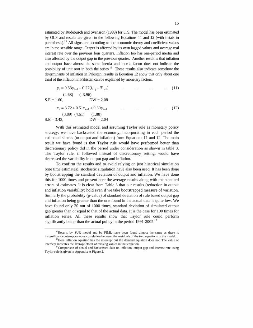
estimated by Rudebusch and Svensson (1999) for U.S. The model has been estimated by OLS and results are given in the following Equations 11 and 12 (with t-stats in parenthesis).15 All signs are according to the economic theory and coefficient values are in the sensible range. Output is affected by its own lagged values and average real interest rate over the previous four quarters. Inflation too has one-period inertia and also affected by the output gap in the previous quarter. Another result is that inflation and output have almost the same inertia and inertia factor does not indicate the possibility of unit root in both the series.16 These results also indicate somehow the determinants of inflation in Pakistan: results in Equation 12 show that only about one third of the inflation in Pakistan can be explained by monetary factors.

)(27.053.0 111 −−− π−−= tttt iyy … … … … (11) (4.68) (–3.96)

S.E = 1.60, DW = 2.08

11 39.051.072.3 −− +π+=π ttt y … … … … (12) (3.89) (4.61) (1.88) S.E = 3.42, DW = 2.04

With this estimated model and assuming Taylor rule as monetary policy strategy, we have backcasted the economy, incorporating in each period the estimated shocks (to output and inflation) from Equations 11 and 12. The main result we have found is that Taylor rule would have performed better than discretionary policy did in the period under consideration as shown in table 3. The Taylor rule, if followed instead of discretionary setting, would have decreased the variability in output gap and inflation.

To confirm the results and to avoid relying on just historical simulation (one time estimates), stochastic simulation have also been used. It has been done by bootstrapping the standard deviation of output and inflation. We have done this for 1000 times and present here the average results along with the standard errors of estimates. It is clear from Table 3 that our results (reduction in output and inflation variability) hold even if we take bootstrapped measure of variation. Similarly the probability (p-value) of standard deviation of rule based output gap and inflation being greater than the one found in the actual data is quite low. We have found only 20 out of 1000 times, standard deviation of simulated output gap greater than or equal to that of the actual data. It is the case for 100 times for inflation series. All these results show that Taylor rule could perform significantly better than the actual policy in the period 1991-2005.17

15Results by SUR model and by FIML have been found almost the same as there is insignificant contemporaneous correlation between the residuals of the two equations in the model.

16Here inflation equation has the intercept but the demand equation does not. The value of intercept indicates the average effect of missing values in that equation.

17Comparison of actual and backcasted data on inflation, output gap and interest rate using Taylor rule is given in Appendix A Figure 2.

16

Table 3

Simulation with the Taylor Rule and the Estimated Model Rule based Actual One Time Bootstrap* p-value**

Average 8.28 9.24 Interest Rate St Deviation 3.53 3.18

Average –0.24 –0.83

Output gap St Deviation 2.47 1.72 1.80 (0.21)(0.21) 0.002

Average 7.36 7.00

Inflation St Deviation 4.31 3.50 4.04 (0.47)(0.47) 0.10

* Average of 1000 values of standard deviations in bootstrap simulation. Standard errors in parenthesis. ** probability of standard deviation with rule being greater than that of actual data. 4.3. Finding Optimal Parameter Values for Pakistan

Now coming to the issue of optimal parameter values (in Taylor rule) for Pakistan, first take the case of optimal inflation target. None of the central banks, with any monetary policy strategy, targets zero inflation.18 Most of the central banks with inflation targeting as monetary policy strategy announce about 2 percent inflation target, though with some tolerance range. Taylor (1993) has also taken inflation target as 2 percent that corresponds to about 2 percent real economic growth of the USA. Pakistan is a developing country with a natural requirement for higher growth rate. Keeping inflation too low may badly affect economic growth. In this paper we have taken seven different inflation targets for simulation from which we have tried to choose the optimal one. 2 percent is taken to simulate the economy with original Taylor rule. Pakistan has experienced about 5 percent real GDP growth over the period 1980-2005. Keeping this in mind and according to the Taylor procedure we have taken 5 percent inflation as another target. As estimated by Khan and Senhadji (2001), threshold level of inflation for developing countries ranges from 7 percent to 11 percent and by Mubarik (2005), this level for Pakistan is 9 percent. So we take five more values, 7 percent–11 percent.

The long run equilibrium real interest rate has been calculated for Pakistan as difference between the average nominal interest rate and inflation over the periods, 1973-2005, 1981-2005 and 1991-2005 as shown in Table 4.19 Results do not show clear pattern over time but nevertheless in all the three periods the average real interest rate is close to zero. So we have taken the value of equilibrium real interest rate as zero for the benchmark and counterfactual simulation is repeated for different values, between one and minus one, of this parameter.

18As central banks are not inflation nutters in King (1997) terminology. 19Judd and Rudebusch (1998) used this methodology for the U.S. data.

17

Table 4

Estimation of Long-run Real Interest Rate 1973–2005 1981–2005 1991–2005

Average Interest Rate 8.34 8.01 8.24 Average CPI Inflation 9.16 7.52 7.89 Average GDPD Inflation 8.92 8.02 8.92 Equilibrium Real Interest Rate* –0.82 0.49 0.35 Equilibrium Real Interest Rate** –0.58 0.00 –0.68 * when inflation is calculated as percentage growth in CPI. ** when inflation is calculated as percentage growth in GDP Deflator.

Finally we have estimated the optimal weights for output and inflation in the Taylor rule for Pakistan. Taylor (1993) has taken equal weights, i.e. 0.5 on both of the objectives, output and inflation. We have taken these weights as a first case. The other two possibilities have been taken as: either all of the weight given to the output stabilisation and no care about inflation deviation and vice versa. First possibility might be more attractive for the developing countries (at least with asymmetric response) where output is the primary and inflation is the secondary issue. The second possibility is obviously more attractive for the stable economies, which put more weight to inflation control or the price stability.20

We have taken these three sets of weights and seven different targets of inflation (total 21 cases) and backcasted the output, inflation and interest rate using estimated parameters and shocks in the macroeconomic model (1.11) and (1.12). We have found that variability in inflation is a decreasing function of the level of inflation target but the variability of output starts increasing above a certain level of inflation target. From the results of all 21 cases, we have selected the best set of parameter values for Pakistan on the basis of the minimised variability in both of the variables, inflation and output and the minimum values of the loss to the society.

The first best set of parameter values with which the rule has performed well in reducing the variability of inflation and output is the case when the central bank puts equal weight to output and inflation stabilisation in the reaction function and targets inflation at 8 percent with zero real interest rate21. The rule with this set of parameter values is given in equation 13. This roughly indicates the optimal level of inflation for Pakistan and the results are consistent with the findings of Mubarik (2005) (with threshold level of inflation for Pakistan as 9 percent) and of Khan and Senhadji (2001) (with threshold range of

20It should be noted however that none of the central banks, even the inflation targeting

ones, practically do this, as inflation targeting is flexible in the sense that central banks put some weight on output stabilisation too, (Svensson 1997; and Ball 1999).

21The coefficient values are same as proposed by Taylor but inflation target is different.

18

inflation for developing countries including Pakistan as 7-11 percent). According to the rule with this set of parameter values, SBP should simply set interest rate equal to the inflation if both inflation and output are on target. But in case of deviation of inflation from the target or that of output from the trend or normal level, the rule proposes the response with a coefficient of 0.5.

)8(5.05.00 −π++π+= tttt yi … … … … (13) or

ttt yi π++−= 5.15.04

Results for the measures of macroeconomic performance by the rule (both in case of historical as well as stochastic simulation) with the first best set of parameter values are given in Table 5. The procedure we have adopted here for comparison is again same as we discussed above in case of actual Taylor rule. From the table it is clear that the variability in output gap and inflation decreases as we move from discretionary policy to the Taylor rule with the first best set of parameter values for Pakistan. However the average values of the variables are somewhat greater in case of following the rule. Again to confirm these results and to find the probability of standard deviation of output and inflation in simulated series being greater than that in the actual series, we have used stochastic simulation to resample the estimated shocks and estimated the standard deviations 1000 times. Our results show that variability of both the objectives remain lower even in the repeated simulation. In 1000 experiments average values of the standard deviations of output gap and inflation are significantly less than those in the actual data.22 It has also been found that the probability of standard deviation of output and inflation, with rule as the monetary policy strategy, being greater than that in the actual data is quite low showing that variability could decrease significantly if the rule has been followed.

Table 5

Simulation with the First Best Set of Parameter Values First Best Set

Actual Historical Stochastic* p-value** Average 8.28 8.08 Interest Rate St Deviation 3.53 3.11 Average -0.24 0.3 Output Gap St Deviation 2.47 1.67 1.72 (0.24) 0.05 Average 7.36 7.88

Inflation St Deviation 4.31 3.49 3.91 (0.47) 0.2

* Average of 1000 values of standard deviations in bootstrap simulation. ** Probability of standard deviation with rule being greater than that of actual data.

22Comparison of actual and simulated data on inflation, output gap and interest rate using

this proposed rule is given in Appendix A, Figure 3.

19

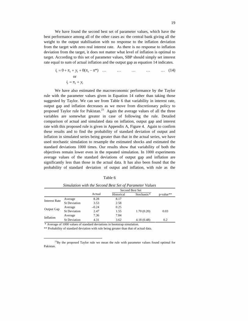
We have found the second best set of parameter values, which have the best performance among all of the other cases as: the central bank giving all the weight to the output stabilisation with no response to the inflation deviation from the target with zero real interest rate. As there is no response to inflation deviation from the target, it does not matter what level of inflation is optimal to target. According to this set of parameter values, SBP should simply set interest rate equal to sum of actual inflation and the output gap as equation 14 indicates.

*)(00 π−π++π+= tttt yi … … … … … (14) or

ttt yi +π=

We have also estimated the macroeconomic performance by the Taylor rule with the parameter values given in Equation 14 rather than taking those suggested by Taylor. We can see from Table 6 that variability in interest rate, output gap and inflation decreases as we move from discretionary policy to proposed Taylor rule for Pakistan.23 Again the average values of all the three variables are somewhat greater in case of following the rule. Detailed comparison of actual and simulated data on inflation, output gap and interest rate with this proposed rule is given in Appendix A, Figure 4. Again to confirm these results and to find the probability of standard deviation of output and inflation in simulated series being greater than that in the actual series, we have used stochastic simulation to resample the estimated shocks and estimated the standard deviations 1000 times. Our results show that variability of both the objectives remain lower even in the repeated simulation. In 1000 experiments average values of the standard deviations of output gap and inflation are significantly less than those in the actual data. It has also been found that the probability of standard deviation of output and inflation, with rule as the

Table 6

Simulation with the Second Best Set of Parameter Values Second Best Set Actual Historical Stochastic* p-value**

Average 8.28 8.17 Interest Rate St Deviation 3.53 2.58 Average –0.24 0.25 Output Gap St Deviation 2.47 1.55 1.70 (0.20) 0.03 Average 7.36 7.84

Inflation St Deviation 4.31 3.62 4.18 (0.48) 0.2

* Average of 1000 values of standard deviations in bootstrap simulation. ** Probability of standard deviation with rule being greater than that of actual data.

23By the proposed Taylor rule we mean the rule with parameter values found optimal for

Pakistan.

20

monetary policy strategy, being greater than that in the actual data is quite low showing that variability could decrease significantly if the rule has been followed.24

4.4. Loss Function and Comparison of Parameter Values

In the last sub-section above, for estimating the optimal parameter values (inflation target and weights on the two objectives) in the Taylor rule for Pakistan, we have used the criterion of minimising the variability in both output and inflation. It is even better if we calculate and compare the loss to the society associated with each set of parameter values. As the loss function includes both the objectives, it can do better job to find optimal parameter values. For estimating the loss function the formula given in equation 6 has been used. For convenience and to compare all the cases on the same ground we have assumed that the society puts equal weight on inflation and the output. We have backcasted the economy with estimated macroeconomic model (estimated parameters and shocks) and taking all sets of parameters (total of 21, as discussed above) one at a time and chose the best set of parameters that minimises the loss function.

By the historical simulation we have again reached the same results as we have found in the comparison of standard deviations individually. We have found that the loss is minimum in case of 8 percent inflation target and equal coefficient values of output and inflation in the reaction function with real interest rate as zero. The second best set of parameter values has been found exactly the same as was proposed by Taylor. However the third best set of parameters contains all the weight given by the monetary authority to the output in the reaction function. Again we have done stochastic simulation to confirm our findings. We have simulated the shocks series 1000 times and then calculated the value of the loss each time and present here (in Table 7) only the average results. We can see from the table that performance of the rule (with either set of parameters) remains better (on average) than in case of actual policy even in 1000 different scenarios. Average loss with each set of parameters has been calculated with a reasonable standard error. Results show that there is very low probability (0.02 in all cases) of loss, associated with the rule, being greater than that with actual policy setting indicating that in 1000 different scenarios 980 times, the rule performed better than discretionary policy with either set of parameter values. Finally we have compared the results of rule with optimal set of parameter values for Pakistan to the one with actual values taken by Taylor. We can see from Table 7 that it is better to follow the Taylor rule with a change in inflation target for Pakistan rather than with that taken by Taylor. It is not surprising as Taylor proposed inflation target for the Fed and not for all the

24However this probability is higher in case of inflation.

21

Table 7

Loss Associated with Different Parameter Values for the Rule Variance Loss to Society Output Inflation Historical Stochastic* p-value** Actual Data 6.10 18.54 12.32 First Best 2.80 12.15 7.48 7.82

(1.92) 0.02

Second Best 2.40 13.11 7.76 8.10 (1.78) 0.02

Taylor Rule 2.94 12.25 7.60 8.26 (1.72) 0.02

* Standard error in parenthesis. ** Probability of loss associated with rule being greater than that of actual data. central banks. Interestingly, in historical simulation, Taylor’s proposed parameter values are better than the second best possibility for Pakistan we have found in this study but opposite is true in stochastic simulation.

4.5. Constrained Numerical Optimisation

We have tried, in section 4.3, to find optimal parameter values in the Taylor rule for Pakistan by choosing the parameter values from a discrete set containing only theoretically or practically feasible values. To countercheck those results, we have done constrained numerical optimisation to find optimal parameter values from a set of continuous parameter values. For this, the loss function 1.6 has been minimised subject to the two constraints in the macroeconomic model (Equations 11 and 12) plus some other constraints on the parameters. With respect to these other constraints we have made the following different cases.

Case-I

(i). Sum of coefficients of output and inflation equals 1.

Case-II

(i). Sum of coefficients of output and inflation equals 1. (ii). In case of only one period shock output gap converges to a level in

the range of -0.1-0.1.

Case-III

(i) Sum of coefficients of output and inflation equals 1. (ii) In case of only one period shock, output gap converges to a level in

the range of -0.1-0.1. (iii) In case of only one period shock, inflation converges to a level in the

range of inflation target ± 0.25.

22

Case-IV

(i) Sum of coefficients of output and inflation equals 1. (ii) In case of only one period shock, output gap converges to a level in

the range of -0.1-0.1. (iii) In case of only one period shock, inflation converges to a level in the

range of inflation target ± 0.50.

By taking two constraints from the transmission mechanism and one set from these five cases each at a time we have found the minimised value of the loss associated with certain parameter values in the rule. Our results in Table 8 show that if we use the set of constraints in the first case then the loss is minimised at about 13.74 percent inflation target along with coefficients of output and inflation as, respectively, 0.42 and 0.58. Weights on output and inflation are almost the same as we have found above in section 4.3 and 4.4 but the results have changed significantly for the target level of inflation: it has increased from 8 percent to 13.74 percent.

Table 8

Loss Minimisation Subject to Different Constraints

Constraints Inflation Target

Coefficient of Output

Coefficient of Inflation Loss

Case-I 13.74 0.42 0.58 7.42

Case-II 8.11 0.42 0.58 7.47

Case-III 7.96 0.41 0.59 7.47

Case-IV 7.91 0.99 0.00 7.76

When we have minimised loss function subject to the second set of constraints where output gap has been forced to converge to zero in response to a one time shock, inflation target has been found again 8 percent and the output and inflation coefficients remained the same as in case I. In the third case, by adding another constraint we have found similar results as in case II. In the next case we have increased just the range around inflation target for convergence and found that results have changed drastically. Inflation target has remained the same (8 percent) but all of the weight has been assigned to output stabilisation.

In summary, we have found here the inflation target as 8 percent and coefficients of output and inflation in most of the cases almost equal (with slightly more weight given to the inflation) and all of the weight given to output stabilisation only in one case. These results confirm our finding, in sub-sections 4.3 and 4.4, of optimal parameter values in the Taylor rule for Pakistan.

23

5. CONCLUSION

In this study the Taylor rule for Pakistan has been estimated for the period 1991-2005 and for the sub-samples of different Governors’ regimes in that period. We have found no evidence that State Bank of Pakistan has ever followed this type of rule. The coefficient of output gap has opposite sign and that of inflation has lesser magnitude than what the Taylor proposed. This might be due to the fact that being central bank of a developing country, SBP focuses on other policy objectives that have not been included in the simple Taylor rule estimation. We have also backcasted the output and inflation assuming Taylor rule as the monetary policy strategy. On the basis of both historical and stochastic simulation, it has been found that macroeconomic performance, in terms of less variability of output and inflation and small value of the loss to the society, could be improved significantly by the rule. We have also tried to estimate optimal parameter values in the rule for Pakistan. We have found that it is optimal for SBP to target 8 percent inflation giving equal weight to both the objectives, output and inflation, in the policy reaction function25.

We conclude here by summarising key messages from the study. First, our results are in line with the modern economic literature on monetary policy rules. Second, despite the lack of pre-requisites for more elaborate policy rules and with weak institutions, developing countries can get benefits by the commitment to simple instrument rules. As argued in this study, simple instrument rules might be a first step for developing countries to move from discretionary policy to more elaborate inflation targeting framework. Third, despite the fact that there are multiple objectives (other than output and inflation) of monetary policy in developing countries, a simple rule that focuses only on the two primary objectives can perform better in these countries. However possibilities of including other objectives in the simple rules may also be explored. Fourth, the parameters in the rule (especially the inflation target) must be adjusted according to the economic conditions of a specific economy.

There are potential topics for future research in this area. Before adopting any policy rule it is essential to explore the monetary policy objectives in a country like Pakistan. Literature on the Taylor rule is still inconclusive on the coefficients of variables (other than output and inflation) in the policy reaction function. So a lot of research is needed to reach some firm conclusions on coefficients of these other variables. There is also a need to explore the ways and possibilities for developing countries to adopt more elaborate inflation targeting framework. In this regard the research is needed on pre-requisites (central bank independence, transparency and accountability of central bank actions) for this type of frameworks. These three notions might be outcome of the elaborate policy rules and not just the pre-requisites for it. Research in this area would be quite beneficial for developing countries where intuitions are not yet strong and there is weak focus on the issues like monetary policy transparency and accountability.

25These results are based on the assumption of zero real interest rate.

24

Appendix A Fig. 2.

Actual and Taylor Rule-induced Short Interest Rate, Output Gap, and Inflation

Actual and Taylor Rule Induced Short Interest Rate

0

3

6

9

12

15

1819

92Q

1

1993

Q1

1994

Q1

1995

Q1

1996

Q1

1997

Q1

1998

Q1

1999

Q1

2000

Q1

2001

Q1

2002

Q1

2003

Q1

2004

Q1

2005

Q1

perc

ent

actual rule induced

Actual and Taylor Rule based Output Gap

-6

-3

0

3

6

9

12

1992

Q1

1993

Q1

1994

Q1

1995

Q1

1996

Q1

1997

Q1

1998

Q1

1999

Q1

2000

Q1

2001

Q1

2002

Q1

2003

Q1

2004

Q1

2005

Q1

perc

ent

actual rule based

Actual and Taylor Rule based Inflation

-30369

121518

1992

Q1

1993

Q1

1994

Q1

1995

Q1

1996

Q1

1997

Q1

1998

Q1

1999

Q1

2000

Q1

2001

Q1

2002

Q1

2003

Q1

2004

Q1

2005

Q1

perc

ent

actual rule based

25

Fig. 3. Actual and First Best Rule-induced Short Interest Rate, Output Gap, and Inflation

Actual and Best Rule-I based Interest Rate

02468

10121416

1992

Q1

1993

Q1

1994

Q1

1995

Q1

1996

Q1

1997

Q1

1998

Q1

1999

Q1

2000

Q1

2001

Q1

2002

Q1

2003

Q1

2004

Q1

2005

Q1

perc

ent

actual rule based

Actual and Proposed Rule-I based Output Gap

-6

-3

0

3

6

9

1992

Q1

1993

Q1

1994

Q1

1995

Q1

1996

Q1

1997

Q1

1998

Q1

1999

Q1

2000

Q1

2001

Q1

2002

Q1

2003

Q1

2004

Q1

2005

Q1

perc

ent

actual rule based

Actual and Proposed Rule-I based Inflation

-202468

10121416

1992

Q1

1993

Q1

1994

Q1

1995

Q1

1996

Q1

1997

Q1

1998

Q1

1999

Q1

2000

Q1

2001

Q1

2002

Q1

2003

Q1

2004

Q1

2005

Q1

perc

ent

actual rule based

26

Fig. 4. Actual and Second Best Rule-induced Short Interest Rate,

Output Gap, and Inflation

Actual and Proposed Rule-II based Interest Rate

02468

1012141618

1992

Q1

1993

Q1

1994

Q1

1995

Q1

1996

Q1

1997

Q1

1998

Q1

1999

Q1

2000

Q1

2001

Q1

2002

Q1

2003

Q1

2004

Q1

2005

Q1

perc

ent

actual rule based

Actual and Proposed Rule-II based Output Gap

-6

-3

0

3

6

9

1992

Q1

1993

Q1

1994

Q1

1995

Q1

1996

Q1

1997

Q1

1998

Q1

1999

Q1

2000

Q1

2001

Q1

2002

Q1

2003

Q1

2004

Q1

2005

Q1

perc

ent

actual rule based

Actual and Proposed Rule-II based Inflation

-30369

121518

1992

Q1

1993

Q1

1994

Q1

1995

Q1

1996

Q1

1997

Q1

1998

Q1

1999

Q1

2000

Q1

2001

Q1

2002

Q1

2003

Q1

2004

Q1

2005

Q1

perc

ent

actual rule based

27

REFERENCES

Ball, Laurence (1999) Efficient Rules for Monetary Policy, International Finance 2:2.

Barro, Robert, and David Gordon (1983a) A Positive Theory of Monetary Policy in a Natural Rate Model. Journal of Political Economy 91, 589–610.

Barro, Robert J., and David B. Gordon (1983b) Rules, Discretion and Reputation in A Model Of Monetary Policy. Journal of Monetary Economics 12:1, 101–121.

Bernanke, Ben S., and Frederic S. Mishkin (1997) Inflation Targeting: A New Framework for Monetary Policy? Journal of Economic Perspectives 11:2, 97–116.

Calvo, Guillermo, and Frederic S. Mishkin (2003) The Mirage of Exchange Rate Regimes for Emerging Market Countries. Journal of Economic Perspectives 17:4, Fall.

Cukierman, A. (2002) Are Contemporary Central Banks Transparent about Economic Models and Objectives and what Difference Does it Make? Federal Reserve Bank of St. Louis Review 84:4, 15–35.

Enders, Walter (2004) Applied Econometric Time Series. John Wiley & Sons, Inc.

Fischer, S. (1993) The Role of Macroeconomic Factors in Growth. Journal of Monetary Economics 32, 485–512.

Henderson, Dale W., and Warwick J. McKibbin (1993) A Comparison of Some Basic Monetary Policy Regimes for Open Economies: Implications of Different Degrees of Instrument Adjustment and Wage Persistence. Carnegie-Rochester Conference Series on Public Policy 39, 221–317.

Judd, P. John, and D. Glenn Rudebusch (1998) Taylor’s Rule and Fed: 1970–1997. FRBSF Economic Review 3.

Khan, M. S., and S. A. Senhadji (2001) Threshold Effects in the Relationship between Inflation and Growth. IMF Staff Papers 48:1.

King, Mervyn (1997) Changes in UK Monetary Policy: Rules and Discretion in Practice. Journal of Monetary Economics 39:1, 81–97.

King, Mervyn A. (1997) The Inflation Target Five Years On. Bank of Engl. Quarterly Bulletin 37:4, 434–442.

Kydland, Finn, and Edward Prescott (1977) Rules Rather Than Discretion: The Inconsistency of Optimal Plans. Journal of Political Economy 85, 473–490.

Levin, Andrew, Volker Wieland, and John C. Williams (1999) Robustness of Simple Monetary Policy Rules under Model Uncertainty, in Monetary Policy Rules. John B. Taylor (ed.) Chicago: Chicago University Press.

Malik, W. Shahid (2006) Money, Output and Inflation: Evidence from Pakistan. The Pakistan Development Review 46:4. (Forthcoming).

Malik, W. Shahid (2007) Monetary Policy Objectives in Pakistan: An Empirical Investigation. Essay in PhD Dissertation, PIDE.

28

McCallum, Bennett T. (1988) Robustness Properties of a Rule for Monetary Policy. Carnegie-Rochester Conference Series on Public Policy 29, 173–204.

McCallum, Bennett T. (2000) The Present and Future of Monetary Policy Rules. International Finance 3, 273–286.

Meltzer, Allan H. (1987) Limits of Short-Run Stabilisation Policy. Economic Inquiry 25, 1–13.

Mubarik, Y. Ali (2005) Inflation and Growth: An Estimate of the Threshold Level of Inflation in Pakistan. SBP-Research Bulletin 1:1.

Rogoff, Kenneth (1985) The Optimal Degree of Commitment to an Intermediate Monetary Target. Quarterly Journal of Economics 100, 1169–1189.

Rudebusch, Glenn D. (2002) Assessing Nominal Income Rules for Monetary Policy with Model and Data Uncertainty. Econ. Journal 112, 402–432.

Rudebusch, Glenn D. and Lars E.O. Svensson (1999) Policy Rules for Inflation Targeting. In John B. Taylor (ed.) Monetary Policy Rules. Chicago: Chicago U. Press. pp. 203–246.

Sharon, Kozicki (1999) How Useful Are Taylor Rules for Monetary Policy? Federal Reserve Bank of Kansas City Economic Review, second quarter.

Svensson Lars E. O. (2002) Inflation Targeting: Should It Be Modeled as an Instrument Rule or a Targeting Rule? European Economic Review 46, 771–780.

Svensson, Lars E. O. (1997). Inflation Forecast Targeting: Implementing and Monitoring Inflation Targets. European Economic Review 41, 1111—1146.

Svensson, Lars E. O. (2003) What is Wrong with Taylor Rules? Using Judgment in Monetary Policy through Targeting Rules. Journal of Economic Literature 41:2, 426–77.

Svensson, Lars E. O. (2005) Monetary Policy with Judgment: Forecast Targeting. International Journal of Central Banking.

Taylor, John B. (1993) Discretion versus Policy Rules in Practice. Carnegie-Rochester Conference Series on Public Policy 39, 195–214.

Taylor, John B. (1999a) Introduction in Monetary Policy Rules. John B. Taylor, ed. Chicago: Chicago U. Press.

Taylor, John B. (1999b) A Historical Analysis of Monetary Policy Rules. In John B. Taylor (ed.) Monetary Policy Rules. Chicago: Chicago U. Press.

Walsh, Carl (1995) Optimal Contracts for Independent Central Bankers. American Economic Review 85, 150—167.

Woodford, Michael (2001) The Taylor Rule and Optimal Monetary Policy. American Economic Review Papers and Proceedings 91, 232–237.