the termination of subprime hybrid and fixed rate … termination of subprime hybrid and fixed ......

Research Division Federal Reserve Bank of St. Louis Working Paper Series

The Termination of Subprime Hybrid and Fixed Rate Mortgages

Anthony Pennington-Cross and

Giang Ho

Working Paper 2006-042A http://research.stlouisfed.org/wp/2006/2006-042.pdf

July 2006

FEDERAL RESERVE BANK OF ST. LOUIS Research Division

P.O. Box 442 St. Louis, MO 63166

______________________________________________________________________________________

The views expressed are those of the individual authors and do not necessarily reflect official positions of the Federal Reserve Bank of St. Louis, the Federal Reserve System, or the Board of Governors.

Federal Reserve Bank of St. Louis Working Papers are preliminary materials circulated to stimulate discussion and critical comment. References in publications to Federal Reserve Bank of St. Louis Working Papers (other than an acknowledgment that the writer has had access to unpublished material) should be cleared with the author or authors.


Anthony Pennington-Cross*

[email protected] or [email protected]. Work: 314-444-8592 Cell: 636-399-0395

and Giang Ho

[email protected]: 314-444-7315

The Federal Reserve Bank of St. Louis Research Division

P.O. Box 442 St. Louis, MO 63166-0442

*Corresponding author: Anthony Pennington-Cross. The views expressed in this research are those of the individual author and do not necessarily reflect the official positions of the Federal Reserve Bank of St. Louis, the Federal Reserve System, and the Board of Governors.

mailto:[email protected]




Abstract

Adjustable rate and hybrid loans have been a large and important component of

subprime lending in the mortgage market. While maintaining the familiar 30-year term the typical adjustable rate loan in subprime is designed as a hybrid of fixed and adjustable characteristics. In its most prevalent form, the first two years are typically fixed and the remaining 28 years adjustable. Perhaps not surprisingly, using a competing risks proportional hazard framework that also accounts for unobserved heterogeneity, hybrid loans are sensitive to rising interest rates and tend to temporarily terminate at much higher rates when the loan transforms into an adjustable rate. However, these terminations are dominated by prepayments not defaults.

JEL Classifications: G21, D14, R29 Keywords: Mortgage, Default, prepayment, Subprime, Adjustable Rate, Hybrid,

Introduction

The mortgage market continues to evolve and provide more access to credit for home

purchase, rate-driven refinancing, and equity extraction-driven refinancing. For example,

mortgage debt dwarfed consumer debt by fourfold in the first quarter of 2005 according

to the American Bankers Association (ABA). Part of this growth can be attributed to the

proliferation of nontraditional mortgage products such as interest-only loans and loans

with little or no documentation of down payment sources or income. In addition, the

growth of the subprime mortgage market has helped introduce credit constrained

households to the mortgage debt market.

Since the introduction of Adjustable Rate Mortgages (ARM) in the early 1980s, however,

recent ARM market shares in the conventional conforming prime market have been fairly

modest (10 to 30 percent from 2003 through 2005) (Fannie Mae 2006). In contrast, the

ARM market share for securitized subprime loans has ranged from just approximately 60

percent to over 80 percent over the same time period. In addition, ARMs are also equally

popular products in the jumbo1 market (Nothaft 2003).

The typical ARM product in subprime is not the traditional one-year ARM indexed to

Treasury bill yields. Instead, a hybrid product that mixes fixed and adjustable attributes

dominates the market place. For example, the ABA reports that two thirds of adjustable

rate purchase loans were 2/28 hybrids. The 2 indicates that the first 2 years of the loan

1 Jumbo loans are loans whose loan amount is greater than the conforming loan limit imposed on Fannie Mae and Freddie Mac. The loan limit is updated annually by the Department of Housing and Urban Development.

1

have a fixed interest rate, while the 28 indicates that the remaining 28 years of the loan

have an adjustable interest rate. Loan Performance data indicate that almost all 2/28

hybrids adjust every six months and are indexed to the London Interbank Offered Rate

(LIBOR).2

To the authors’ knowledge, this paper provides the first empirical examination of the

performance of 2/28 hybrid mortgages in the subprime market. A competing risk

framework is employed that allows for the dependence of the two types of termination

(default and prepayment) and controls for unobserved heterogeneity without assuming a

shape to the unobserved distribution. In addition, a large national data set of loans

originated from 1998-2005 is used that includes loans backed by real estate and

securitized in the asset-backed securities market by private firms (private label). The

performance of subprime 30-year hybrid loans is compared with concurrently originated

subprime 30-year fixed rate loans.

Literature on Adjustable and Hybrid Rate Loans

Both the theoretical and empirical literature on the termination of mortgages through

prepayment and default has been well developed and we will not dwell on it in this paper.

Instead we will extend the empirical literature by examining hybrid performance in the

securitized potion of the subprime market.

2 London Interbank Offered Rate (or LIBOR) is a daily reference rate based on the interest rates at which banks offer to lend unsecured funds to other banks in the London wholesale (or "interbank") money market.

2

ARMs provide unique benefits and costs from both the borrower and the lender’s

perspective. Unlike Fixed Rate Mortgages (FRMs), ARMs potentially impose payment

shocks on the borrower as interest rates increase. On the other hand, if interest rates

decrease, at the prescribed adjustment date, the borrower will automatically benefit from

a lower payment.3 In other words, the borrower using an ARM takes on interest rate risk

that the lender usually faces when originating or investing in a fixed rate product. In

terms of pricing lenders provide lower initial interest rates to compensate the borrower

for bearing more of the interest rate risk (Bruekner 1986; Sa-Aadu and Sirmans 1989). In

practice there is continuum of interest rate risk sharing. For example, caps and floors on

how much rates can change over the life of the mortgage or in each adjustment period can

be used to shield the borrower from large or fast adjustments in underlying interest rates.

Therefore, while holding lender-expected returns constant, the more interest rate risk the

borrower takes on, the lower the expected cost for the borrowing should be. This feature

can make ARMs more affordable and easier to qualify for than FRMs. Many ARMs also

have initial interest rates that are below the fully indexed rate (the teaser rate). Therefore,

even if the index is constant through time, the interest rate and monthly payment paid by

the ARM borrower using a teaser will increase until the rate is fully adjusted (index plus

the margin or spread).

There is evidence that under asymmetric information a separating equilibrium exists

where high-risk borrowers choose to finance using an ARM (Posey and Yavas 2001).

Therefore, it should not be surprising that the subprime market is associated with much

3 This benefit or cost will be realized only to the extent that the underlying index changes through time and the interest rate is reset.

3

higher rates of ARM usage than the conventional prime market. It is also widely

believed that borrowers who expect to move or prepay their mortgage in the near future

are likely to self-select into ARMs (Bruekner 1986; Bruekner and Follain 1988; Dhillon,

Shilling, and Sirmans 1987). Given the structure of the hybrid mortgage and the low

costs of refinancing, hybrid borrowers may plan to refinance at the end of the fixed rate

period to avoid the impact of teasers or higher interest rates on the required monthly

payment. Consistent with these issues, our estimation data set (discussed below)

indicates that on average hybrid borrowers have lower credit scores, provide a smaller

down payment, and are more likely to have a prepayment penalty on the loan. In

addition, on average hybrid loans terminate through both default and prepayment at

elevated rates. It will be an empirical question as to whether these observed differences

are explained by borrower and location characteristics or reflect a unique hybrid specific

termination profile.

There is a fairly substantial empirical literature on the termination of ARMs. In general,

the traditional ARM seems to respond in a similar fashion to the economic and financial

incentives to default or prepay a mortgage. For example, default is more likely when

there is negative or low equity in a home and prepayments are more likely when

prevailing interest on mortgages have declined. However, there is some mixed evidence

on the impact of teaser rates and other ARM-specific terms on terminations (Ambrose

and LaCour-Little 2001; Calhoun and Deng 2002; Green and Shilling 1997; Vanderhoff

1996; Bruekner and Follain 1988; Cunningham and Capone 1990). In the paper most

similar to our own, Amborse, LaCour-Little, and Huszar (2005) examine the performance

4

of 3/27 hybrid loans from one lender using a sample of 181 observed defaults on over

2,000 loans originated in 1995 and 1996. They find that the time period when the loan

converts from a fixed to an adjustable rate is associated with a substantial and permanent

increase in the conditional hazard of default and with a substantial but temporary increase

in the conditional hazard of prepayment.

Our following empirical investigation contributes to the literature by (1) including a

much larger sample of hybrids, (2) providing direct comparisons with concurrently

originated FRMs, (3) including many lenders, (4) covering the subprime market, and (5)

using more recent data.

Competing Risks Estimation with Unobserved Heterogeneity

A loan can terminate through either default or prepayment – two options that compete

with each other to be the first observed event. We jointly model the probability of default

and prepayment in a competing risks proportional hazard framework that also accounts

for the unobserved factors that influence the termination of the mortgages. We employ

the empirical approach used by Yu (2006), who investigates bank bankruptcy and

mergers. This method is based on the work by Han and Hausman (1990), Sueyoshi

(1992), and McCall (1996).

Let TD, TP, and TC be the duration to default, prepayment, and the end of the sample

period (censored), respectively. For a mortgage j with j=1,…,N the first realized

termination time is observed, Tj=min{TP,TD,TC}. To explain the termination history of

the loans, we control for both observed heterogeneity X(t), which can be time-constant or

5

time-variant, and unobserved heterogeneity (ΘD, ΘP), which has the joint density g(θD,

θP) and is assumed to be independent of X(t). The dependence between the two risks

(default and prepay) conditioning on X is related directly to the distribution of the

unobserved characteristics -- that is, the correlation of the unobserved heterogeneity

parameters.

The cause-specific hazard function (the probability of termination at time t conditioned

on survival to time t) is defined as

tXtTtTtPXt PDr

tPD

r

Δ≥Δ≤≤

=+→Δ

),,,|(lim),,|(0

θθθθλ , (1)

for r=D, P.

For our empirical estimation, the hazards are specified in the following form

})()(exp{),,|( 0 rrr

PDr tXtXt θβλθθλ ++= , (2)

where r=D, P and denotes the baseline hazard for risk r. The loan subscript j has

been dropped for convenience. We investigate two possible forms of the baseline hazard

functions. In the polynomial form, the baseline is parameterized as a quadratic function

of the loan age: (for identification purpose is fixed at 0).

Alternatively, the shape of the baseline might be imposed by employing a standard such

as the “PSA experience” and shifting the PSA up or down to match the observed level of

terminations in the subprime mortgage market.

)(0 trλ

22100 )( ttt rrrr αααλ ++= r

0α

4

4 The Public Securities Association (PSA) has attempted to standardize market assumptions about the pattern of mortgage default and prepayments, with terminations assumed to occur at some chosen multiple of the standard path. By the standard default assumption, 100% SDA assumes a linear rise from 0% to 0.6% for the first 30 months, constant at peak value for the next 30 months, linear decline to 0.03% over the next 60 months, and constant at 0.03% for remaining life. By the standard prepayment model, 100%

6

Since the outcomes are assumed to be independent of each other when conditioning on

observed and unobserved characteristics, the conditional survival function is defined as:

}.)),,|(),,|((exp{

),,,|(*),,|(),,,|(

),,|(

0dsXsXs

XtTPXtTPXtTP

XtS

PDPt

PDD

PDPPDD

PD

PD

θθλθθλ

θθθθθθ

θθ

+=

≥≥=≥=

∫

(3)

If we denote the indicator variables for termination by default ID and prepay IP, then a

typical loan j has the following likelihood function:

,),().,,|()|( PDPDPDjjjjj ddgXTLXTLD P

θθθθθθ∫ ∫Θ Θ= (4)

where

[ ] [ ]}.)),,|(),,|((exp{

*),,|(*),,|(),,|(

0∫ +−

=j

PD

T

PDP

PDD

IPDjj

PIPDjj

DPDjj

dsXsXs

XTXTXTL

θθλθθλ

θθλθθλθθ (5)

Since termination and mortgage payments occur at discrete intervals of the same length

(monthly frequency), we make the assumption that the time-varying covariates X(t) are

constant within each interval. In other words, if there are T* potential termination times,

then X(t - ∆) = X(t), 0 < ∆ < 1, t = 1,…,T*. As noted by Sueyoshi (1992), this is a natural

assumption given the inherent discreteness of sampling and the lack of a priori

knowledge about the evolution of the covariates over time. Under this condition (5) is

reduced to

PSA assumes (1) a linear rise from 0% to 6% for the first 30 month and (2) a constant rate at 6% for remaining life. These rates are annualized.

7

[ ] [ ]

.)),,|(),,|((exp

*),,|(.),,|(),,|(

1 ⎭⎬⎫

⎩⎨⎧

+−

=

∑=

j

PD

T

sPD

PPD

D

IPDjj

PIPDjj

DPDjj

XsXs

XTXTXTL

θθλθθλ

θθλθθλθθ (6)

For estimation purpose we assume that the unobserved heterogeneities follow a discrete

probability distribution with M points of support (or mass points), pm, where∑ .

The approach estimates the size of M distinct groups of loans with distinct probabilities

of default and prepay. Further, following Dong and Koppelman (2003) and Yu (2006), to

ensure that the probabilities lie within [0, 1] and sum up to 1, we use a logistic

transformation on the mass-point estimates

=

=M

mmp

11

),/( ∑= mm qqm eep (7)

where -∞ < qm < ∞ and q1 is normalized to 0.5

Data

Our empirical analysis investigates the performance of FRM and hybrid mortgages to

determine whether and how they respond differently to mortgage characteristics and

time-varying financial and economic incentives to terminate the loan. Data are from the

LoanPerformance Asset Backed Securities loan-level database and represent only the

securitized portion of the subprime market. The loans included in our data sets are

originated between 1998 and 2005, and performance is followed monthly for up to eight

years until the end of 2005. Besides end-of-sample censoring, the data are also left-

censored in the sense that loans are often allowed to season for various amounts of time

before becoming part of the securities pool. To facilitate the estimation of the hazard

5 The likelihood function is defined and maximized in SAS/OR 9.1 for Windows in Proc NLP. While the data is proprietary, the code is available on request from the authors.

8

functions we limit our samples to the 2-month seasoned loans only. The FRM sample

consists of over 72,000 30-year fixed rate single-family mortgages (purchases and

refinances), and the ARM sample includes over 101,000 2/28 hybrid loans.6 The 2/28

hybrid instruments make up the majority of the adjustable rate mortgage universe,

averaging over 68 percent of all ARMs in our data between 1998 and 2005.

To help describe the data and differences between hybrids and FRMs, we conducted a

preliminary analysis of our sample data using the non-parametric Kaplan-Meier

estimators. The Kaplan-Meier method has the advantage that it can account for right-

censored data. Specifically, we estimate the Kaplan-Meier cause-specific hazard

functions (Figures 1 and 2), the cumulative default and prepay functions (Figure 3), and

the survival function (Figure 4) for both hybrid and fixed rate loans by loan age.7 A loan

is considered to default if it becomes “Real Estate Owned (REO)” property or if

foreclosure proceedings are initiated. A loan is prepaid when the balance becomes zero

and in the prior month the loan was either current or delinquent. We focus on the first 60

months because, as the loans get older, there are fewer observations and the censorship

problem also becomes more severe, making the estimates less reliable. The figures show

6 Rates are fixed for the first 2 years and adjustable every 6 months and indexed to the 6-month LIBOR for the next 28 years. Approximately 99% of the 2/28 ARMs have a rate reset frequency of 6 months and are indexed to the 6-month LIBOR, so we focus on this dominant type. 7 Assuming hazards occur at discrete times, tj = t0 + j*∆ with j = 1,…,J. Define the number of loans “at risk” at time tj, nj, to be those that have reached the time point tj without being censored or terminated. Define drj to be the number of terminations due to cause r at time point tj. The Kaplan-Meier estimate of the hazard function and the survival function are

jn

rjdjtr =)(λ̂ , ∏

≤−= ⎟

⎟⎠

⎞⎜⎜⎝

⎛tjt jn

jdtKMS 1)(ˆ .

The cumulative incidence function for cause r is ∑=

=j

i itKMSitrjtrI1

).(ˆ)(ˆ)(ˆ λ

9

that for our loan samples, the 2/28 hybrids tended to default more than the 30-year fixed

rate mortgages, with the monthly default rate reaching a peak of 1.5 percent at around the

30th month. About 10 percent of FRMs (20 percent of hybrids) have defaulted five years

after origination. Hybrids prepaid much faster than FRMs during the two-year period

after the first adjustment date (25th month). In fact, the peak conditional monthly hazard

of prepayment is above 12 percent in the first month that the loans change over to

adjustable rates. Approximately 20 percent of hybrids survived after three years while

40 percent of FRMs survived. In the following sections we will incorporate explanatory

variables in a competing risks analysis to better understand the default and prepay

patterns of adjustable and fixed rate mortgages.

To estimate the conditional monthly default and prepay probabilities specified in

equation (2) for hybrid and fixed rate loans, we include various mortgage and market

characteristics as our covariates. Table 1 describes the variables and Table 2 provides

some summary statistics for our estimation samples. Due to the different nature of the

fixed and adjustable rate mortgage contracts we use a different set of covariates for each

loan product.

The mortgage variables common to the two models are borrower’s credit score at

origination, fico, the current loan-to-value ratio, cltv, and indicators of loan

documentation and prepayment penalty status, lndoc and ppen. The FICO score

measures the consumer’s ability to meet prior financial obligations, and therefore

borrowers with higher credit scores are expected to default less often. However, the

10

relationship between credit scores and the likelihood of prepayment is unclear. The fixed

rate loans in our sample have a higher average FICO score (664) than the adjustable rate

loans (603). Given these loans are included in ABS securities, the market has treated

them as not-prime or subprime loans. It appears that the securitized FRM subprime

represents the better or A- segment of the subprime market. In contrast, the FICO scores

on the ARM loans are low enough that these loans are most likely to represent the higher

cost segments such as the B&C segment of subprime. The current loan-to-value ratio,

cltv, is calculated using the reported outstanding loan balance in each month and the

house value updated by the OFHEO metropolitan area house price index.8 This variable

measures the equity position of the borrower and can be a strong predictor of both default

and prepay probabilities. When a loan is in low or negative equity (higher cltv), it is

often “in the money” to default and put the mortgage back to the lender or investor. On

the other hand, substantial positive equity compensates for other risks such as weak credit

history, making it easier to refinance the mortgage. In our samples, the hybrid loans have

slightly higher loan-to-value ratio than the fixed rate loans (78 percent vs. 73 percent).

About 19 percent of the hybrids in the sample provided limited or no documentation

(lndoc) of income or down payment sources. In contrast, the figure is twice as high for

the FRMs. Lack of documentation may indicate additional risks associated with future

incomes and thus is expected to increase default probabilities. In addition, in 40 percent

of fixed rate loan-months there is a prepayment penalty in effect (ppen), compared with

8 Other studies have created a variable representing the probability that the home is in negative equity. However, the parameters necessary to calculate this variable are available to the public only at the state level. We prefer to use the metropolitan area index to more accurately reflect local market conditions and include an additional volatility measure of the index itself.

11

almost 70 percent for hybrid rate loans. These penalties make it more costly to prepay a

mortgage, thus in their presence the prepayment probabilities should be lower.

Prepayment penalties have also been found to increase default probabilities (Quercia,

Stegman and Davis 2005), possibly because they increase the cost of prepaying relative

to default when a loan becomes delinquent.

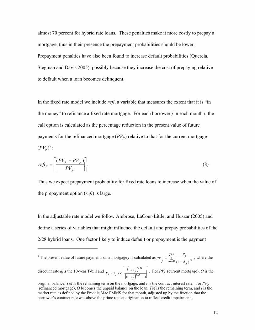
In the fixed rate model we include refi, a variable that measures the extent that it is “in

the money” to refinance a fixed rate mortgage. For each borrower j in each month t, the

call option is calculated as the percentage reduction in the present value of future

payments for the refinanced mortgage (PVjr) relative to that for the current mortgage

(PVjc)9:

⎥⎥⎦

⎤

⎢⎢⎣

⎡ −=

jc

jrjcjt PV

PVPVrefi

)(. (8)

Thus we expect prepayment probability for fixed rate loans to increase when the value of

the prepayment option (refi) is large.

In the adjustable rate model we follow Ambrose, LaCour-Little, and Huszar (2005) and

define a series of variables that might influence the default and prepay probabilities of the

2/28 hybrid loans. One factor likely to induce default or prepayment is the payment

9 The present value of future payments on a mortgage j is calculated as ∑

= +=

TM

m mjd

jP

jPV

0 )1(, where the

discount rate dj is the 10-year T-bill and ( )( ) ⎥

⎥⎦

⎤

⎢⎢⎣

⎡

−+

+∗=

11

1

TMji

TMji

OjijP . For PVjc (current mortgage), O is the

original balance, TM is the remaining term on the mortgage, and i is the contract interest rate. For PVjr (refinanced mortgage), O becomes the unpaid balance on the loan, TM is the remaining term, and i is the market rate as defined by the Freddie Mac PMMS for that month, adjusted up by the fraction that the borrower’s contract rate was above the prime rate at origination to reflect credit impairment.

12

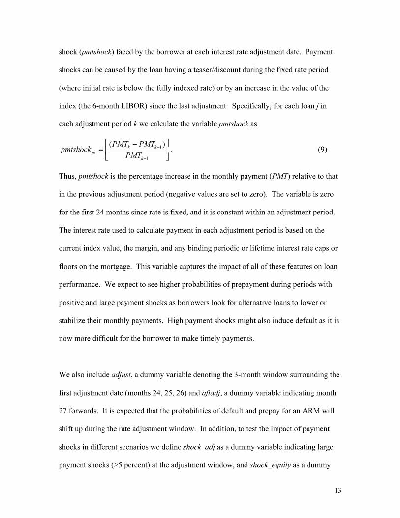
shock (pmtshock) faced by the borrower at each interest rate adjustment date. Payment

shocks can be caused by the loan having a teaser/discount during the fixed rate period

(where initial rate is below the fully indexed rate) or by an increase in the value of the

index (the 6-month LIBOR) since the last adjustment. Specifically, for each loan j in

each adjustment period k we calculate the variable pmtshock as

⎥⎦

⎤⎢⎣

⎡ −=

−

−

1

1 )(

k

kkjk PMT

PMTPMTpmtshock . (9)

Thus, pmtshock is the percentage increase in the monthly payment (PMT) relative to that

in the previous adjustment period (negative values are set to zero). The variable is zero

for the first 24 months since rate is fixed, and it is constant within an adjustment period.

The interest rate used to calculate payment in each adjustment period is based on the

current index value, the margin, and any binding periodic or lifetime interest rate caps or

floors on the mortgage. This variable captures the impact of all of these features on loan

performance. We expect to see higher probabilities of prepayment during periods with

positive and large payment shocks as borrowers look for alternative loans to lower or

stabilize their monthly payments. High payment shocks might also induce default as it is

now more difficult for the borrower to make timely payments.

We also include adjust, a dummy variable denoting the 3-month window surrounding the

first adjustment date (months 24, 25, 26) and aftadj, a dummy variable indicating month

27 forwards. It is expected that the probabilities of default and prepay for an ARM will

shift up during the rate adjustment window. In addition, to test the impact of payment

shocks in different scenarios we define shock_adj as a dummy variable indicating large

payment shocks (>5 percent) at the adjustment window, and shock_equity as a dummy

13

variable indicating large payment shocks (>5 percent) coupled with low equity (cltv>90

percent). Option theory indicates that payment shocks associated with low or negative

equity should be more strongly associated with defaults than shocks with large amounts

of equity. However, lender forbearance and the use of short sales (sale price less than

outstanding balance on loan) may temper this expected impact.

Several market variables are tested in both FRM and hybrid models: the metropolitan

area unemployment rate (unemp), and house price and interest rate volatility (varhpi and

varint/varindex). Higher unemployment rates proxy for labor market conditions and the

chance that the borrower will be unemployed. Therefore, we should expect higher

probabilities of default when unemployment rates are high. As indicated by option

theory, the volatility proxies are included to measure the extent that it makes sense to

delay entering default or prepayment even if it is in the money to do so in the current

period (Kau and Kim 1994). In particular, if house prices are volatile it may make sense

to wait to see if the value of the option increases in the future (larger negative equity).

The same logic applies to interest rates. If interest rates are volatile it may make sense to

wait for it to become more deeply in the money in the future to refinance. To measure

the volatility of interest rates the 6-month LIBOR (the index) is used for hybrids and 1-

year Treasury yields for FRMs. Lastly, in the hybrid model we include a measure of the

spread between the prevailing 30-year fixed rate and the prevailing 1-year ARM rate

(spread) to proxy for the benefits of shifting from an ARM to an FRM.

14

Results

The results largely meet expectations in terms of statistical significance and coefficient

signs. In terms of the traditional risk drivers (equity, interest rates, and credit scores)

both hybrids and FRMs react in the same direction, although with different magnitudes.

The most striking difference between hybrids and FRMs occurs during the first rate

adjustment period when the loan converts from a fixed rate to an adjustable rate. In this

period both defaults and prepayments are elevated even without any payment shock.

Tables 3 through 6 report the estimated coefficients for four different specifications.

Specifications I and III do not allow for unobserved heterogeneity, while II and IV do.

Specifications I and II estimate a parametric (quadratic) baseline, while III and IV include

a proportionally shifted PSA baseline. In general, coefficient estimates are sensitive to the

introduction of unobserved heterogeneity parameters but are very similar in both baseline

specifications. The variable that measures the extent that a change in interest rates

increases monthly payments (pmtshock) is especially sensitive to unobserved

characteristics. This result may be because the explanatory variables do not include

important borrower-specific variables such as the amount of debt and wealth available to

soften the impact of payment shocks. One drawback of the quadratic baseline is that it

relies on an increasingly small sample of defaulted loans as the loans get older. This

shrinking data set is not due to right censoring but instead due to the very low survivor

rate, as previously shown using the Kaplan-Meier hazards, of subprime loans. Therefore,

we will focus on the estimates using the PSA baseline.

15

The unobserved parameter estimates are all significant at the 5 percent level or higher and

show substantial unobserved heterogeneity in default and prepayment for both hybrid and

fixed rate specifications. However, the organization of the loans into low and high

default and prepayment groups differs across the two loan types. For the FRMs the

majority (76 percent) of loans are in the high default and high prepayment groups. For

the hybrids the majority of loans (64 percent) are in the high default and low prepayment

groups. This indicates that unobserved loan and borrower characteristics may be

different in the hybrid and fixed rate environments. In addition, note that the location

parameter estimates (θ ’s) are positive using the PSA baseline. This indicates that the

PSA baseline is being proportionally shifted up for all loan groups and reflects the high

termination rates of subprime loans.

The Baseline of Hybrid and Fixed Rate Loans Figures 5 and 6 provide a graphical representation of the PSA baselines using conditional

monthly probability estimates. Figure 5 represents the estimated baselines for the

average fixed and the average hybrid loan as the loan ages. For FRMs as the loan ages

the probability of default increases to a high of 0.43 percent and the probability of

prepayment increases to a high of 5.04 percent. Both of these are multiples of the

standard PSA (0.05 percent for default and 0.50 percent for prepayment). In terms of

default, the hybrids have a substantially higher probability of default regardless of the age

of the loan. In terms of prepayment it is not until the adjustment period when the rate

shifts from fixed to adjustable that hybrid prepayment probabilities are substantially

higher than those of FRMs (almost 6 percent relative to 4.5 percent). However, after the

adjustment period the probability of prepayment for the hybrids drops substantially below

16

the FRM level. Figure 6 controls for borrower and loan characteristics by using the

characteristics of the average hybrid on the FRM coefficient estimates. After this

adjustment, in terms of default probabilities the difference between the hybrid and FRM

is greatly diminished. Hybrid default probabilities do increase a little faster in the first

two years, but after the first adjustment time period the default baseline for the hybrid and

FRM are very similar. In terms of prepayment the hybrid probabilities do increase faster

during the first two years and increase substantially during the adjustment period.

However, after the adjustment period the hybrids prepay at a lower rate for the rest of the

life of the loan. Figure 7 plots this information from a cumulative perspective. The

figure emphasizes that there is very little difference between hybrid and FRM default

baselines. In fact, at the end of five years almost exactly 18 percent of the loans have

defaulted and almost 70 percent of loans have prepaid regardless of loan type. The major

difference is that the hybrids tend to prepay earlier (before and during the first rate

adjustment).

Perhaps surprisingly, estimates of baseline cumulative termination rates using hybrid

prime loans are very similar to the subprime termination rates. For example, Ambrose,

LaCour-Little, and Huszar (2005) estimated that after 5 years just over 70 percent of the

loans had prepaid and approximately 25 percent had defaulted. However, in contrast to

our results they found that after the conversion (first adjustment time period) default

probabilities were elevated and prepayments returned to their parametric baseline hazard.

17

Figure 5 through 7 are driven by the variables adjust, which measures the impact of the

first adjustment time period when the loan changes from fixed to adjustable rates, and

aftadj, which controls for the remaining time period when the loan is an ARM. All other

variables were evaluated at their means. This implies that the baselines shown assume

that interest rates are essentially constant and as a result there is no payment shock when

the rate adjusts. The coefficient estimates and the elasticity estimates in Tables 7 and 8

indicate that the termination of hybrid loans is also sensitive to the size of the payment

shock. In particular, a one-standard-deviation increase in the payment shock is associated

with a 48.9 percent increase in the probability of prepaying and a 23.6 percent increase in

the probability of default. This is strong evidence that in rising rate environments even

more subprime borrowers try to find an alternative mortgagee; and, if they do not, the

likelihood of default is also elevated.

Figures 8 and 9 focus on the first adjustment time period and introduce a large payment

shock (greater than 5 percent increase) during the adjustment period when the borrower

has a good proportion of equity in the home (shock_adj) and when the borrower has little

equity in the home (shock_equity). The monthly conditional probabilities are normalized

to 1 in month 23 and then followed until the 36th month of the loans life. Figures 8 and 9

also assume that the second adjustment period, which starts in month 31, has no payment

shock (interest rates are held constant from month 25 forward in time). Reflecting the

impact of adjust and aftadj, if there is no payment shock in the first adjustment period

both defaults and prepayments are elevated temporarily before returning to a slightly

lower level. However, contrary to the impact of large payment shocks in later adjustment

18

periods, if there is a big payment shock during the first adjustment period as reflected by

shock_adj both defaults and prepayments are depressed for a few months, but are slightly

elevated for the next four months. However, if the big shock happens to a borrower with

low equity (shock_equity) in the home the depressing effect in the first few months is

lessened and the rise in termination in the last four months of the first adjustment period

are substantially elevated. In fact, the probability of default and prepayment is more than

twice as high relative to month 23. Therefore, it is the classic combination of the

borrower not having enough equity on the home in conjunction with a trigger event that

can dramatically increase the termination of hybrid loans. The only difference for the

hybrid, as compared with the FRM, is that the trigger event is designed into the contract

and is contingent on the path of future interest rates.

Other Covariates – X(t)

This section discusses the impact of the non-baseline related variables on the termination

of hybrid and fixed rate loans. The discussion focuses on Tables 7 and 8, which provide

standardized elasticity estimates based on one-standard-deviation increases of continuous

variables and increases from 0 to 1 for dummy variables while holding all other variables

at their means.

Consistent with prior literature on mortgage performance, higher credit scores at

origination are associated with large decreases in the probability of default and modest

increases in the probability of prepaying. However, the magnitude of the response in

terms of default is much smaller for the hybrid loans (-32 percent for hybrids versus -53

percent for FRMs). Again, consistent with prior empirical literature, the amount of

19

equity in the home strongly impacts both the probability of default and prepayment.

Loans with low or negative equity are much more likely to default and substantially less

likely to prepay. However, as shown in Figure 10, hybrids are less sensitive to this

impact in terms of defaulting and more sensitive to this impact in terms of prepaying. In

addition, rising interest rates are associated with lower probabilities of prepayment. Also,

as expected, low documentation is associated with higher probabilities of default and

prepayment penalties are associated with lower probabilities of prepayment. The impact

of unemployment rates is fairly small or statistically insignificant.

Variables measuring the impact of the volatility of interest rates and house prices also

meet expectations and are consistent with options theory (volatility leads to delaying

exercising an option). For example, when house prices are more volatile the probability

of default declines when interest rates are volatile, as measured using LIBOR or Treasury

bills, and the probability of prepaying is slightly retarded.

Conclusion

The theories of mortgage selection and pricing suggests that high-risk borrowers who

expect to move or refinance their mortgage will self select into using adjustable rate

mortgages. This paper finds strong empirical evidence supporting these theories. First,

adjustable rate loans are much more prevalent in the subprime market, where by

definition borrowers are more high-risk. In addition, the credit scores for hybrid loans

are substantially lower than for fixed rate loans on average (602 versus 664), even within

subprime. Also consistent with self-selection, the profile of hybrid terminations through

default becomes much more similar to fixed rate terminations after controlling for credit

20

scores, down payments, and economic conditions. Second, we find strong evidence that

subprime loans do terminate quickly. For example, Kaplan-Meier estimates indicate that

by two years (two and a half years) the majority of subprime hybrid rate loans (fixed rate

loans) have terminated. However, competing risk results indicate that by the end of five

years in a neutral rate environment both fixed and the hybrid loans will be approximately

70 percent terminated, which is very similar to hybrid estimates in the prime market.

The most prevalent type of adjustable rate loans in subprime is the hybrid loan, which

mixes fixed rate characteristics with adjustable rate characteristics. For example,

typically the rate in the first 2 years is fixed and the rate in the remaining 28 (2/28 hybrid)

is adjustable, with a rate reset every six months indexed to LIBOR. In a market where

transaction costs are low and an environment where the best outcome for the borrower is

to get out of the loan as fast as possible, the 2/28 hybrid is a natural medium or even

short-term loan that helps to keep payments low for a few years. After a few years the

borrower can refinance into another loan, which could be another hybrid or even a prime

loan. Therefore, it should be no surprise over the first 2 years of the 2/28 hybrid that the

loans default and prepay more often than fixed rate loans even after controlling for key

characteristics such as down payments and credit scores. Moreover, the time period

when the loan converts from a fixed to adjustable rate is associated with a dramatic and

temporary increase in prepayments and a modest and temporary increase in defaults.

However, for those loans that survive past this first adjustment period, the baseline

termination probabilities for the 2/28 hybrids are actually lower than the termination

probabilities for similar subprime fixed rate loans.

21

While the baselines reveal the unique termination profile of the hybrids, it does not

include the impact of any rising interest rates. By design hybrids subject borrowers to

payment shocks when interest rates rise or when an initial rate teaser is phased out.

Hybrids are sensitive to these payment shocks. The competing risks model results

indicate that a one-standard-deviation increase in the size of the shock is associated with

an almost 50 percent increase in the probability of prepaying and more than a 25 percent

increase in the probability of defaulting. As a result, in an increasing interest rate

environment we should expect to see elevated rates of default and prepayment in the

subprime mortgage market.

22

References

Ambrose, B. W., M. LaCour-Little, and Z. R. Huszar. 2005. A Note on Hybrid Mortgages. Real Estate Economics 33: 765-782.

Ambrose, B. W. and M. LaCour-Little. 2001. Prepayment Risk in Adjustable Rate Mortgage Subject to Initial Year Discounts: Some New Evidence. Real Estate Economics 29: 305-327.

Bruekner, J. K. 1986. The Pricing of Interest Rate Caps and Consumer Choice in the Market for Adjustable-Rate Mortgages. Housing Finance Review 5: 119-136.

Bruekner, J. K. and J. R. Follain. 1988. The Rise and Fall of an ARM: An Econometric Analysis of Mortgage Choice. The Review of Economics and Statistics 70: 93-102.

Calhoun, C. A. and Y. Deng. 2002. A Dynamic Analysis of Fixed- and Adjustable-Rate Mortgage Terminations. Journal of Real Estate Finance and Economics 24: 9-33.

Cunningham, D. F. and C. A. Capone, Jr. 1990. The Relative Termination Experience of Adjustable to Fixed-Rate Mortgages. The Journal of Finance 45: 1687-1703.

Dhillon, U., J. D. Shilling, and C. F. Sirmans. 1987. Choosing Between Fixed and Adjustable Rate Mortgages. Journal of Money, Credit, and Banking 19: 260-267.

Dong, X., F. S. Koppelman. 2003. Comparison of Methods Representing Heterogeneity in Logit Models. Presented at the 10th International Conference on Travel Behaviour Research, Lucerne, 10-15 August 2003.

Fannie Mae. 2006. U.S. Housing and Mortgage Market Outlook. FundingNotes For Fannie Mae‘s Investors and Dealers, March 2006.

Green R. K. and J. D. Shilling. 1997. The Impact of Initial-Year Discounts on ARM Prepayments. Real Estate Economics 25: 373-385.

Han, A. and J. Hausman. 1990. Flexible Parametric Estimation of Duration and Competing Risk Models. Journal of Applied Econometrics 5: 1-28. Kau, J. and T. Kim. 1994. Waiting to Default: The Value of Delay. American Real Estate and Urban Economics Association 22: 539-51.

McCall, B. P. 1996. Unemployment Insurance Rules, Joblessness, and Part-Time Work. Econometrica 64: 647-682.

Nothaft, F. 2003. Will Interest Change Lead to Higher ARM Share? Special Commentary from the Office of the Chief Economist. Available at http://www.freddiemac.con/news/finance/commentary/sp-comm_092203.html.

Posey, L. L. and A. Yavas. 2001. Adjustable and Fixed Rate Mortgages as a Screening Mechanism for Default Risk. Journal of Urban Economics 49: 54-79.

Quercia, R.G., M. Stegman and W. Davis. 2005. The Impact of Predatory Loan Terms on Subprime Foreclosures: The Special Case of Prepayment Penalties and Balloon Payments. University of North Carolina Kenan-Flagler Business School, January 25, 2001.

23

Sa-Aadu, J. and C. F. Sirmans. 1989. The Pricing of Adjustable Rate Mortgage Contracts. Journal of Real Estate Finance and Economics 2: 253-266.

Sueyoshi, G. T. 1992. Semi-parametric Proportional Hazards Estimation of Competing Risks Models with Time-varying Covariates. Journal of Econometrics 51: 25-58.

Vanderhoff, J. 1996. Adjustable and Fixed Rate Mortgage Termination, Option Values and Local Market Conditions: An Empirical Analysis. Real Estate Economics 24: 379-406.

Yu, X. 2006. Competing Risk Analysis of Japan’s Small Financial Institutions. Stanford University, Department of Economics working paper.

24

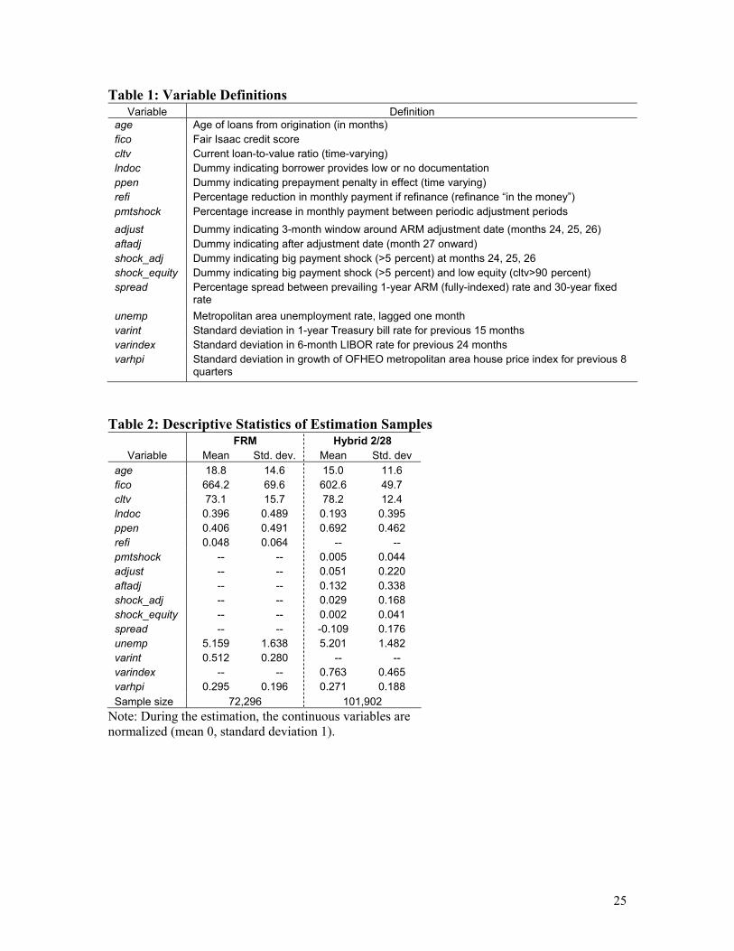
Table 1: Variable Definitions Variable Definition

age Age of loans from origination (in months) fico Fair Isaac credit score cltv Current loan-to-value ratio (time-varying) lndoc Dummy indicating borrower provides low or no documentation ppen Dummy indicating prepayment penalty in effect (time varying) refi Percentage reduction in monthly payment if refinance (refinance “in the money”) pmtshock Percentage increase in monthly payment between periodic adjustment periods adjust Dummy indicating 3-month window around ARM adjustment date (months 24, 25, 26) aftadj Dummy indicating after adjustment date (month 27 onward) shock_adj Dummy indicating big payment shock (>5 percent) at months 24, 25, 26 shock_equity Dummy indicating big payment shock (>5 percent) and low equity (cltv>90 percent) spread Percentage spread between prevailing 1-year ARM (fully-indexed) rate and 30-year fixed

rate unemp Metropolitan area unemployment rate, lagged one month varint Standard deviation in 1-year Treasury bill rate for previous 15 months varindex Standard deviation in 6-month LIBOR rate for previous 24 months varhpi Standard deviation in growth of OFHEO metropolitan area house price index for previous 8

quarters

Table 2: Descriptive Statistics of Estimation Samples

FRM Hybrid 2/28 Variable Mean Std. dev. Mean Std. dev

age 18.8 14.6 15.0 11.6 fico 664.2 69.6 602.6 49.7 cltv 73.1 15.7 78.2 12.4 lndoc 0.396 0.489 0.193 0.395 ppen 0.406 0.491 0.692 0.462 refi 0.048 0.064 -- -- pmtshock -- -- 0.005 0.044 adjust -- -- 0.051 0.220 aftadj -- -- 0.132 0.338 shock_adj -- -- 0.029 0.168 shock_equity -- -- 0.002 0.041 spread -- -- -0.109 0.176 unemp 5.159 1.638 5.201 1.482 varint 0.512 0.280 -- -- varindex -- -- 0.763 0.465 varhpi 0.295 0.196 0.271 0.188 Sample size 72,296 101,902

Note: During the estimation, the continuous variables are normalized (mean 0, standard deviation 1).

25

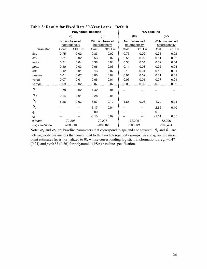
Table 3: Results for Fixed Rate 30-Year Loans – Default Polynomial baseline PSA baseline (I) (II) (III) (IV)

No unobserved heterogeneity

With unobserved heterogeneity



Parameter Coef. Std. Err. Coef. Std. Err. Coef. Std. Err. Coef. Std. Err. fico -0.75 0.02 -0.83 0.02 -0.75 0.02 -0.76 0.02 cltv 0.51 0.02 0.53 0.02 0.55 0.02 0.51 0.02 lndoc 0.31 0.04 0.38 0.04 0.33 0.04 0.32 0.04 ppen 0.10 0.03 -0.06 0.03 0.11 0.03 0.05 0.03 refi 0.12 0.01 0.13 0.02 0.10 0.01 0.13 0.01 unemp 0.01 0.02 0.00 0.02 0.01 0.02 0.01 0.02 varint 0.07 0.01 0.06 0.01 0.07 0.01 0.07 0.01 varhpi -0.09 0.02 -0.07 0.02 -0.09 0.02 -0.09 0.02

1α 0.78 0.02 1.42 0.04 -- -- -- --

2α -0.24 0.01 -0.28 0.01 -- -- -- --

1θ -6.28 0.03 -7.67 0.10 1.85 0.03 1.70 0.04

2θ -- -- -5.17 0.04 -- -- 2.62 0.10 q1 -- -- 0.00 -- -- 0.00 q2 -- -- -0.13 0.02 -- -- -1.14 0.05 # loans 72,296 72,296 72,296 72,296 Log Likelihood -200,910 -200,382 -200,121 -199,494

Note: 1α and 2α are baseline parameters that correspond to age and age squared. 1θ and 2θ are heterogeneity parameters that correspond to the two heterogeneity groups. q1 and q2 are the mass point estimates (q1 is normalized to 0), whose corresponding logistic transformations are p1=0.47 (0.24) and p2=0.53 (0.76) for polynomial (PSA) baseline specification.

26

Table 4: Results for Fixed Rate 30-Year Loans – Prepay Polynomial baseline PSA baseline (I) (II) (III) (IV)





Parameter Coef. Std. Err. Coef. Std. Err. Coef. Std. Err. Coef. Std. Err. fico 0.09 0.01 0.09 0.01 0.09 0.01 0.09 0.01 cltv -0.09 0.01 -0.15 0.01 -0.02 0.01 -0.12 0.01 lndoc 0.00 0.01 0.03 0.02 0.04 0.01 0.01 0.01 ppen -0.36 0.01 -0.55 0.02 -0.35 0.01 -0.50 0.02 refi 0.12 0.00 0.12 0.01 0.09 0.00 0.13 0.00 unemp 0.05 0.00 0.05 0.01 0.06 0.00 0.06 0.01 varint -0.02 0.01 -0.04 0.01 -0.05 0.01 -0.03 0.01 varhpi 0.14 0.00 0.14 0.01 0.14 0.00 0.14 0.01

1α 0.49 0.01 1.12 0.02 -- -- -- --

2α -0.12 0.00 -0.19 0.01 -- -- -- --

1θ -3.75 0.01 -4.94 0.03 2.09 0.01 1.75 0.02

2θ -- -- -2.57 0.03 -- -- 3.45 0.03 q1 -- -- 0.00 -- -- 0.00 q2 -- -- -0.13 0.02 -- -- -1.14 0.05 # loans 72,296 72,296 72,296 72,296 Log Likelihood -200,910 -200,382 -200,121 -199,494


27

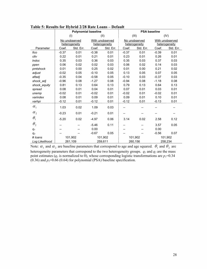
Table 5: Results for Hybrid 2/28 Rate Loans – Default Polynomial baseline PSA baseline (I) (II) (III) (IV)





Parameter Coef. Std. Err. Coef. Std. Err. Coef. Std. Err. Coef. Std. Err. fico -0.37 0.01 -0.38 0.01 -0.37 0.01 -0.39 0.01 cltv 0.22 0.01 0.21 0.01 0.23 0.01 0.26 0.01 lndoc 0.35 0.03 0.36 0.03 0.35 0.03 0.37 0.03 ppen 0.06 0.02 0.02 0.03 0.06 0.02 0.14 0.03 pmtshock 0.01 0.00 0.25 0.02 0.01 0.00 0.21 0.02 adjust -0.02 0.05 -0.10 0.05 0.13 0.05 0.07 0.05 aftadj -0.35 0.04 -0.58 0.05 -0.10 0.03 -0.37 0.03 shock_adj -0.96 0.08 -1.27 0.08 -0.94 0.08 -1.18 0.08 shock_equity 0.81 0.13 0.64 0.13 0.79 0.13 0.64 0.13 spread 0.08 0.01 0.04 0.01 0.07 0.01 0.03 0.01 unemp -0.02 0.01 -0.02 0.01 -0.02 0.01 -0.02 0.01 varindex 0.08 0.01 0.09 0.01 0.09 0.01 0.10 0.01 varhpi -0.12 0.01 -0.12 0.01 -0.12 0.01 -0.13 0.01

1α 1.03 0.02 1.09 0.03 -- -- -- --

2α -0.23 0.01 -0.21 0.01 -- -- -- --

1θ -5.20 0.02 -4.97 0.06 3.14 0.02 2.58 0.12

2θ -- -- -5.46 0.11 -- -- 3.57 0.05 q1 -- -- 0.00 -- -- 0.00 q2 -- -- -0.67 0.05 -- -- -0.56 0.07 # loans 101,902 101,902 101,902 101,902 Log Likelihood 261,109 259,611 260,156 258,234


28

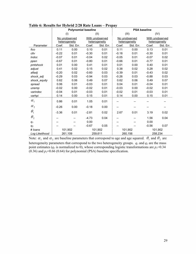
Table 6: Results for Hybrid 2/28 Rate Loans – Prepay Polynomial baseline PSA baseline (I) (II) (III) (IV)





Parameter Coef. Std. Err. Coef. Std. Err. Coef. Std. Err. Coef. Std. Err. fico 0.11 0.00 0.10 0.01 0.11 0.00 0.13 0.01 cltv -0.22 0.01 -0.30 0.01 -0.18 0.01 -0.30 0.01 lndoc -0.07 0.01 -0.04 0.02 -0.05 0.01 -0.07 0.02 ppen -0.67 0.01 -0.80 0.01 -0.66 0.01 -0.77 0.01 pmtshock 0.01 0.00 0.41 0.01 0.01 0.00 0.40 0.01 adjust 0.41 0.02 0.15 0.02 0.38 0.02 0.28 0.02 aftadj -0.20 0.02 -0.60 0.03 -0.39 0.01 -0.43 0.02 shock_adj -0.29 0.03 -0.94 0.03 -0.26 0.03 -0.88 0.03 shock_equity 0.62 0.06 0.49 0.07 0.62 0.06 0.49 0.07 spread 0.06 0.01 -0.03 0.01 0.04 0.01 -0.04 0.01 unemp -0.02 0.00 -0.02 0.01 -0.03 0.00 -0.02 0.01 varindex -0.04 0.01 -0.03 0.01 -0.02 0.01 -0.03 0.01 varhpi 0.14 0.00 0.15 0.01 0.14 0.00 0.15 0.01

1α 0.86 0.01 1.05 0.01 -- -- -- --

2α -0.26 0.00 -0.18 0.00 -- -- -- --

1θ -3.36 0.01 -2.81 0.02 2.67 0.01 3.19 0.02

2θ -- -- -4.73 0.04 -- -- 1.56 0.04 q1 -- -- 0.00 -- -- 0.00 q2 -- -- -0.67 0.05 -- -- -0.56 0.07 # loans 101,902 101,902 101,902 101,902 Log Likelihood 261,109 259,611 260,156 258,234


29

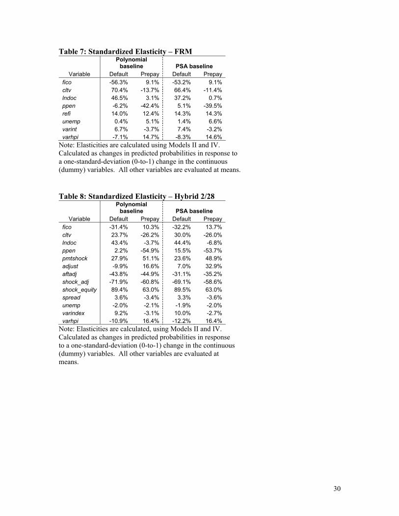
Table 7: Standardized Elasticity – FRM

Polynomial

baseline PSA baseline Variable Default Prepay Default Prepay

fico -56.3% 9.1% -53.2% 9.1% cltv 70.4% -13.7% 66.4% -11.4% lndoc 46.5% 3.1% 37.2% 0.7% ppen -6.2% -42.4% 5.1% -39.5% refi 14.0% 12.4% 14.3% 14.3% unemp 0.4% 5.1% 1.4% 6.6% varint 6.7% -3.7% 7.4% -3.2% varhpi -7.1% 14.7% -8.3% 14.6%

Note: Elasticities are calculated using Models II and IV. Calculated as changes in predicted probabilities in response to a one-standard-deviation (0-to-1) change in the continuous (dummy) variables. All other variables are evaluated at means. Table 8: Standardized Elasticity – Hybrid 2/28

Polynomial

baseline PSA baseline Variable Default Prepay Default Prepay

fico -31.4% 10.3% -32.2% 13.7% cltv 23.7% -26.2% 30.0% -26.0% lndoc 43.4% -3.7% 44.4% -6.8% ppen 2.2% -54.9% 15.5% -53.7% pmtshock 27.9% 51.1% 23.6% 48.9% adjust -9.9% 16.6% 7.0% 32.9% aftadj -43.8% -44.9% -31.1% -35.2% shock_adj -71.9% -60.8% -69.1% -58.6% shock_equity 89.4% 63.0% 89.5% 63.0% spread 3.6% -3.4% 3.3% -3.6% unemp -2.0% -2.1% -1.9% -2.0% varindex 9.2% -3.1% 10.0% -2.7% varhpi -10.9% 16.4% -12.2% 16.4%

Note: Elasticities are calculated, using Models II and IV. Calculated as changes in predicted probabilities in response to a one-standard-deviation (0-to-1) change in the continuous (dummy) variables. All other variables are evaluated at means.

30

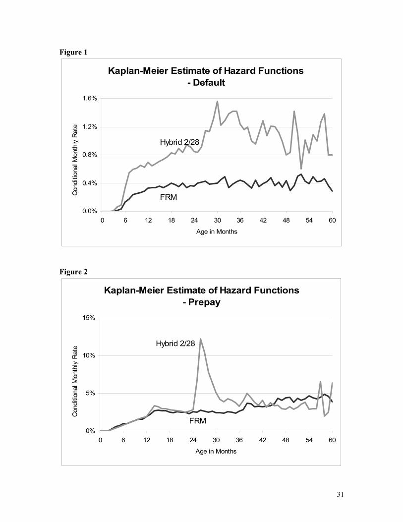
Figure 1

Kaplan-Meier Estimate of Hazard Functions - Default

0.0%

0.4%

0.8%

1.2%

1.6%

0 6 12 18 24 30 36 42 48 54 60

Age in Months

Con

ditio

nal M

onth

ly R

ate

Hybrid 2/28

FRM

Figure 2

Kaplan-Meier Estimate of Hazard Functions - Prepay

0%

5%

10%

15%

0 6 12 18 24 30 36 42 48 54 60

Age in Months

Con

ditio

nal M

onth

ly R

ate

Hybrid 2/28

FRM

31

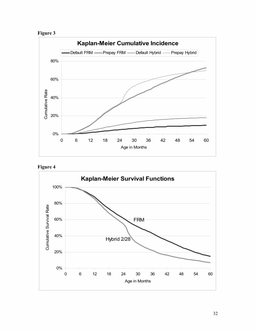
Figure 3

Kaplan-Meier Cumulative Incidence

0%

20%

40%

60%

80%

0 6 12 18 24 30 36 42 48 54 60Age in Months

Cum

ulat

ive

Rat

e

Default FRM Prepay FRM Default Hybrid Prepay Hybrid

Figure 4

Kaplan-Meier Survival Functions

0%

20%

40%

60%

80%

100%

0 6 12 18 24 30 36 42 48 54 60

Age in Months

Cum

ulat

ive

Sur

viva

l Rat

e

Hybrid 2/28

FRM

32

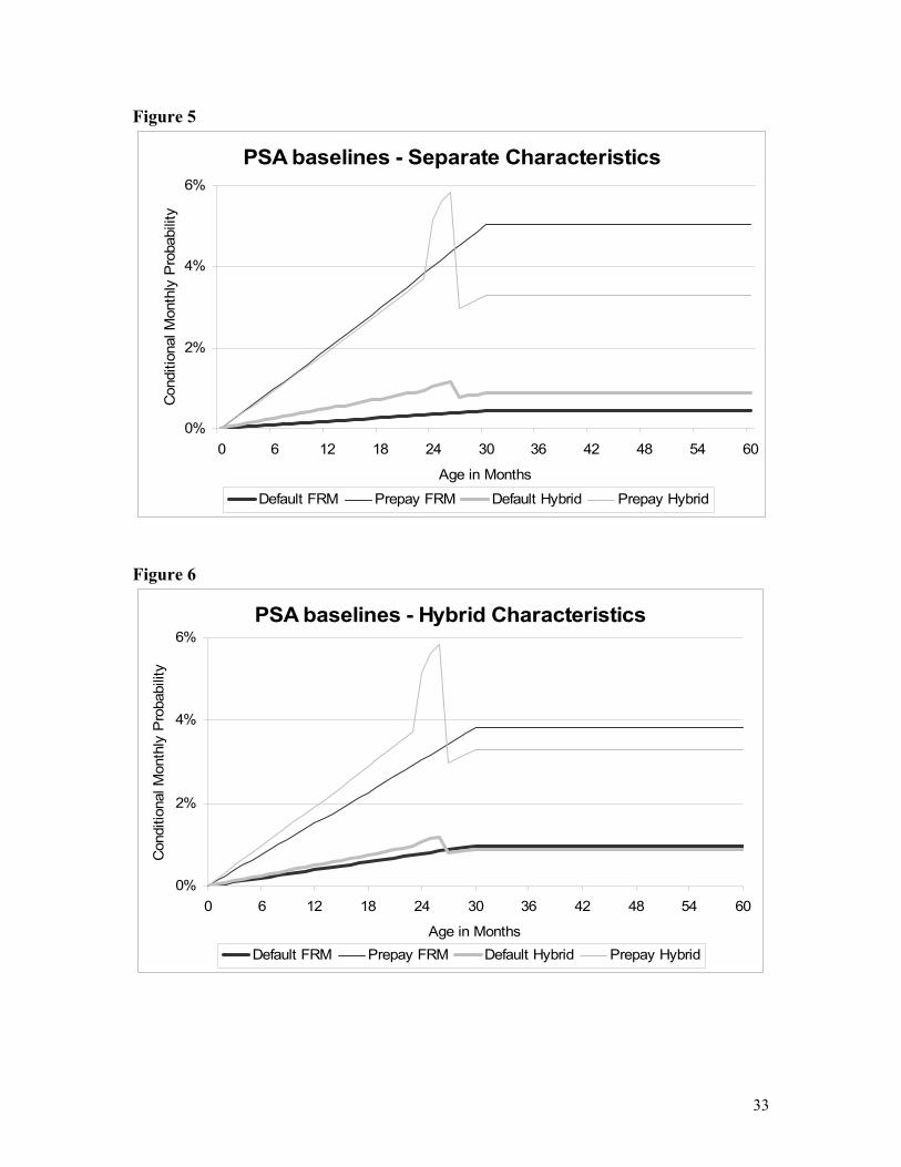
Figure 5

PSA baselines - Separate Characteristics

0%

2%

4%

6%

0 6 12 18 24 30 36 42 48 54 60

Age in Months

Con

ditio

nal M

onth

ly P

roba

bilit

y


Figure 6

PSA baselines - Hybrid Characteristics

0%

2%

4%

6%

0 6 12 18 24 30 36 42 48 54 60

Age in Months

Con

ditio

nal M

onth

ly P

roba

bilit

y


33

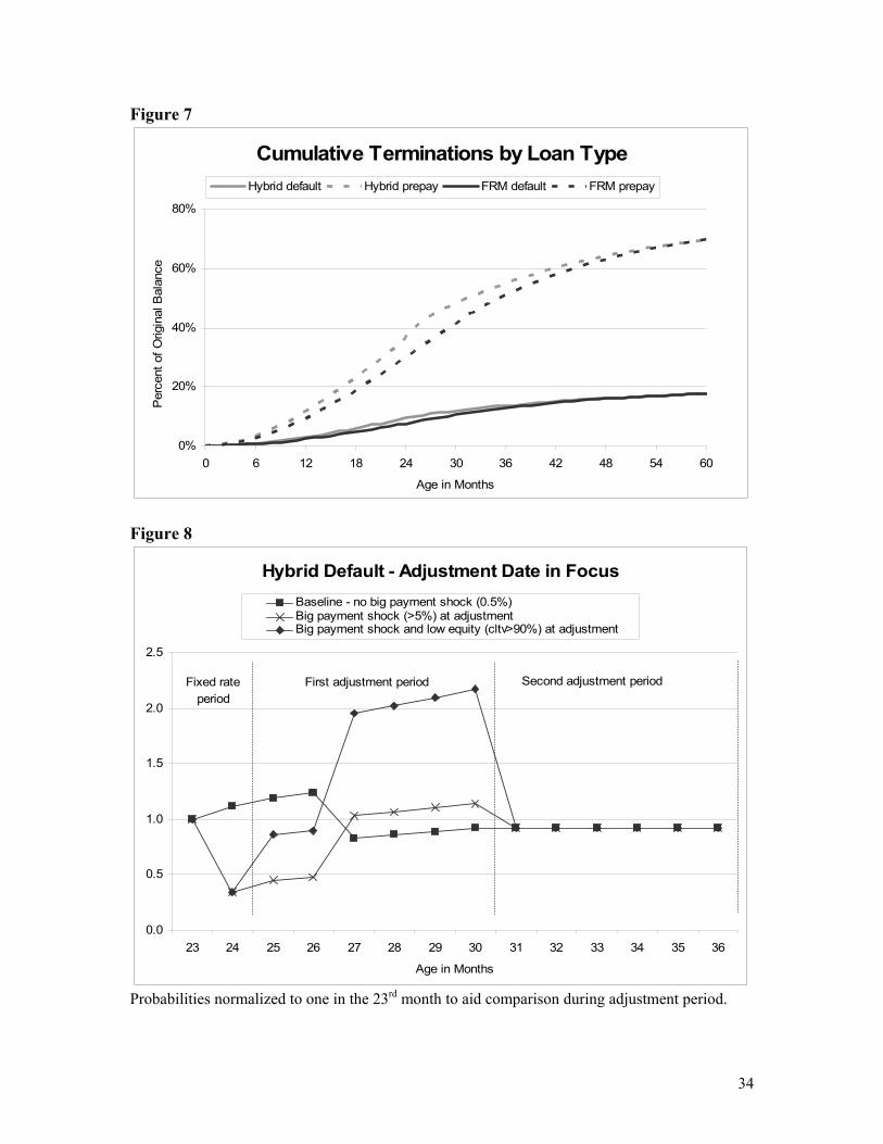
Figure 7

Cumulative Terminations by Loan Type

0%

20%

40%

60%

80%

0 6 12 18 24 30 36 42 48 54 60

Age in Months

Per

cent

of O

rigin

al B

alan

ce

Hybrid default Hybrid prepay FRM default FRM prepay

Figure 8

Hybrid Default - Adjustment Date in Focus

0.0

0.5

1.0

1.5

2.0

2.5

23 24 25 26 27 28 29 30 31 32 33 34 35 36

Age in Months

Baseline - no big payment shock (0.5%)Big payment shock (>5%) at adjustmentBig payment shock and low equity (cltv>90%) at adjustment

First adjustment period Second adjustment periodFixed rate period

Probabilities normalized to one in the 23rd month to aid comparison during adjustment period.

34

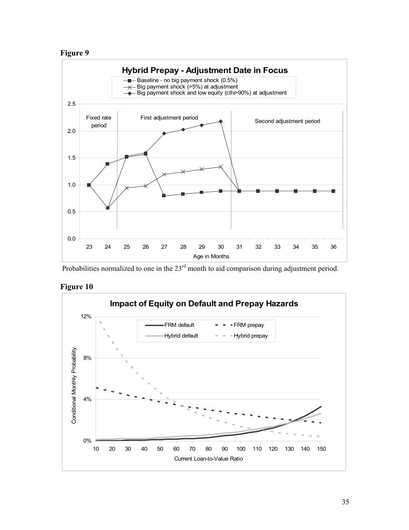
Figure 9

Hybrid Prepay - Adjustment Date in Focus

0.0

0.5

1.0

1.5

2.0

2.5

23 24 25 26 27 28 29 30 31 32 33 34 35 36

Age in Months

Baseline - no big payment shock (0.5%)Big payment shock (>5%) at adjustmentBig payment shock and low equity (cltv>90%) at adjustment

First adjustment period Second adjustment periodFixed rate period

Probabilities normalized to one in the 23rd month to aid comparison during adjustment period. Figure 10

Impact of Equity on Default and Prepay Hazards

0%

4%

8%

12%

10 20 30 40 50 60 70 80 90 100 110 120 130 140 150

Current Loan-to-Value Ratio

Con

ditio

nal M

onth

ly P

roba

bilit

y

FRM default FRM prepay

Hybrid default Hybrid prepay

35

the termination of subprime hybrid and fixed rate … termination of subprime hybrid and fixed ......

Documents