1

The Theoretical Structure of

Producer Willingness to Pay Estimates

Samuel D. Zapata

Graduate Research Assistant, The John E. Walker Department of Economics, Clemson

University, Clemson, SC 29634-0313, szapata@clemson.edu

Carlos E. Carpio

Assistant Professor, The John E. Walker Department of Economics, Clemson University,

Clemson, SC 29634-0313, ccarpio@clemson.edu

Selected Paper prepared for presentation at the Agricultural & Applied Economics

Association’s 2012 AAEA Annual Meeting, Seattle, Washington, August 12-14, 2012

Copyright 2012 by Samuel D. Zapata and Carlos E. Carpio. All rights reserved. Readers may

make verbatim copies of this document for non-commercial purposes by any means, provided

that this copyright notice appears on all such copies.

2

The Theoretical Structure of

Producer Willingness to Pay Estimates

Samuel D. Zapata

Graduate Research Assistant, The John E. Walker Department of Economics, Clemson

University, Clemson, SC 29634-0313, szapata@clemson.edu

Carlos E. Carpio

Assistant Professor, The John E. Walker Department of Economics, Clemson University,

Clemson, SC 29634-0313, ccarpio@clemson.edu

Abstract

This paper analyzes the theoretical underpinnings of producers’ willingness to pay

(WTP) for novel inputs. In addition to conceptualizing the WTP function for

producers, we derive its comparative statics and demonstrate the use of these

properties to estimate input quantities demanded, outputs supplied, and price

elasticities. We also discuss implications of the comparative statics results for the

specification of empirical producer WTP models and survey design.

Key words: Cobb-Douglas production function, contingent valuation, price elasticities, new

technologies, survey design.

3

1. Introduction

Producers and agribusinesses are constantly seeking new technologies or inputs with novel

attributes that can help them reduce production costs and increase revenues. However, the novel

nature of these products also means that prospective suppliers do not have data from actual

markets to estimate the potential demand for these new technologies or inputs. To estimate

producers’ demands, suppliers of these novel factors can rely on stated preference methods such

as contingent valuation.

Contingent valuation, a survey-based methodology, was initially developed to elicit the

value (i.e., willingness to pay, WTP) that people place on non-market goods and services. This

elicitation methodology has been used primarily in the assessment of individuals’ WTP for

environmental services (e.g., Carson et al., 1995; Boyle, 2003; Carson and Hanemann, 2005;

Zapata et al., 2012). More recent applications of contingent valuation methodologies are found in

other areas such as health economics (e.g., Diener et al., 1998; Krupnick et al., 2002), real estate

appraising (e.g., Breffle et al., 1998; Banfi et al., 2008; Lipscomb, 2011), art valuation (e.g.,

Thompson et al., 2002), and agribusiness (e.g., Lusk and Hudson, 2004).

The majority of empirical and theoretical contingent valuation literature has focused on

the consumer side, rather than on the producer side. For example, applications of contingent

valuation on agribusiness are mainly related to consumers’ WTP for neoteric products, food

quality enhancements, or specific attributes (e.g., Lusk, 2003; Carpio and Isengildina-Massa,

2009). However, little conceptual or empirical work has been conducted to understand the

monetary value that producers and agribusinesses place on new production factors.

The purpose of this paper is to extend the literature regarding producers’ WTP for new

technologies or inputs. More specifically, we derive the producers’ WTP function (also called

4

variation function) and its corresponding comparative statics, which have implications for the

specification of empirical WTP models and survey design. In fact, we demonstrate the use of

these properties to estimate the quantity demanded of novel inputs, the quantity supplied of the

output and price elasticities. Hence, another contribution of this paper is the establishment of a

link between traditional demand analyses (with emphasis on the estimation of price and income

elasticities) and contingent valuation studies (with a focus on estimating a mean WTP value).

This is important because agribusinesses are mainly interested in estimating market demand for

novel products and market reaction measures such as price elasticities.

This paper is laid out as follows: Section 2 presents a brief literature review of contingent

valuation and its uses in agribusiness. Section 3 discusses the theoretical structure of the WTP or

variation function and comparative statics. Empirical implications of the theoretical results are

presented in Section 4. Finally, Section 5 provides some brief conclusions. All proofs are

presented in the Appendix.

2. Literature Review

The contingent valuation methodology was first proposed and implemented by Davis (1963) who

designed a hypothetical scenario to assess the economic value of recreational possibilities of

Maine’s forests. Since then, great progress has been achieved in empirical procedures and

theoretical foundations of the contingent valuation method (Hanemann, 1984; Cameron, 1988).

Contingent valuation methods are now widely used by researchers and government agencies as

crucial tools in the assessment of environmental benefits (Carson et al., 1995; Boyle, 2003;

Carson and Hanemann, 2005).

The theoretical foundations of discrete choice models for contingent valuation were

developed by Hanemann (1984) and Cameron (1988). Both authors assumed that individual

5

responses arose from discrete instances of utility maximization, which would imply a consumer

WTP function with properties derived from neoclassical utility functions. However, the Cameron

approach facilitates the derivation of comparative statics of the WTP function and is consistent

with discrete choice and continuous valuation function models (Whitehead, 1995). Consider

Whitehead’s (1995) definition of consumers WTP for a policy with a goal to change the quality

of goods consumed from to :

(1) [ ( )] [ ( )]

[ ( )] ,

where [ ] and ( ) are the individual’s expenditures and indirect utility functions, respectively;

is the vector of good prices; is a vector of quality of goods consumed; and is income.

Comparative statics of the WTP function can be derived by taking derivatives of equation (1)

with respect to the variables of interest. For example, Whitehead (1995) shows that the effect of

the ith

input price on consumer WTP is

(2)

( )

( ),

where ( ) and

( ) are Marshallian demand functions before and after the quality

change, respectively, and , , is the partial derivative of the expenditure function with

respect to indirect utility (

[ ]); , and all arguments other than environment

quality level are suppressed for simplicity (Whitehead, 1995).

Comparative statics results, such as those presented in (2), can be used to theoretically

interpret the results of contingent valuation empirical models or predict the change in demand for

goods after quality improvement (McConnell, 1990; and Whitehead, 1995).

6

One limitation of this theoretical work is its focus on the WTP of consumers.1 Moreover,

to the best of our knowledge, the implications of these properties for empirical work have been

largely ignored. Similarly, on the empirical side, the vast majority of contingent valuation

literature has focused on the consumer side rather than on producers.

Few empirical studies are found on the literature regarding the use of contingent

valuation methods for producers. For example, the only studies found in the agribusiness

literature related with this subject include the estimation of producers’ WTP for information

under risk (Roe and Antonovitz, 1985), crop insurance (Patrick, 1988), agricultural extension

services (Whitehead et al., 2001, Budak et al., 2010), and novel technologies or inputs (Kenkel

and Norris, 1995; Hudson and Hite, 2003). Overall, as the literature review shows, little

conceptual and empirical work has been conducted to understand the monetary value that

producers place on new production factors.

3. Theoretical Model and Comparative Statics

Theoretical Framework

The derivation of the producer WTP function for novel factors of production is based on the

model used by McConnell and Bockstael (2005) to explain the effects of environmental changes

in the firm production process. The theoretical model proposed in this paper allows the analysis

of producers’ WTP for a change in quality of any factor of production and not only a change in

the environmental goods or services as in McConnell and Bockstael’s model (2005). Suppose

1 McConnell and Bockstael (2005) developed several theoretical models with the aim to conceptualize and measure

the economic value that firms place on environmental services. However, the main emphasis of this work has been

on elucidating the economic costs and benefits of environmental changes that influence production rather than

explaining the economic value producers place on novel factors of production.

7

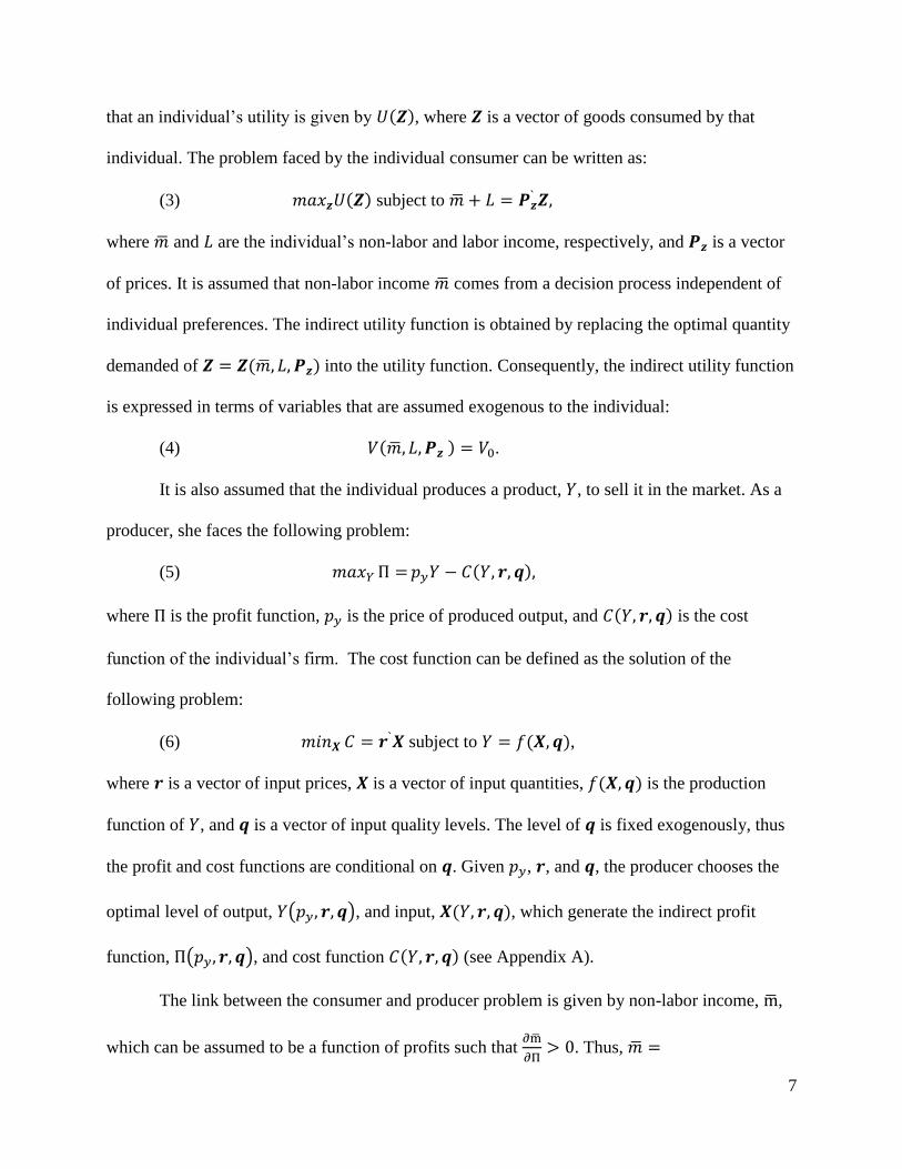
that an individual’s utility is given by ( ), where is a vector of goods consumed by that

individual. The problem faced by the individual consumer can be written as:

(3) ( ) subject to

where and are the individual’s non-labor and labor income, respectively, and is a vector

of prices. It is assumed that non-labor income comes from a decision process independent of

individual preferences. The indirect utility function is obtained by replacing the optimal quantity

demanded of ( ) into the utility function. Consequently, the indirect utility function

is expressed in terms of variables that are assumed exogenous to the individual:

(4) ( ) .

It is also assumed that the individual produces a product, , to sell it in the market. As a

producer, she faces the following problem:

(5) ( )

where is the profit function, is the price of produced output, and ( ) is the cost

function of the individual’s firm. The cost function can be defined as the solution of the

following problem:

(6) subject to ( ),

where is a vector of input prices, is a vector of input quantities, ( ) is the production

function of , and is a vector of input quality levels. The level of is fixed exogenously, thus

the profit and cost functions are conditional on . Given , , and , the producer chooses the

optimal level of output, ( ), and input, ( ), which generate the indirect profit

function, ( ), and cost function ( ) (see Appendix A).

The link between the consumer and producer problem is given by non-labor income, ,

which can be assumed to be a function of profits such that

. Thus,

8

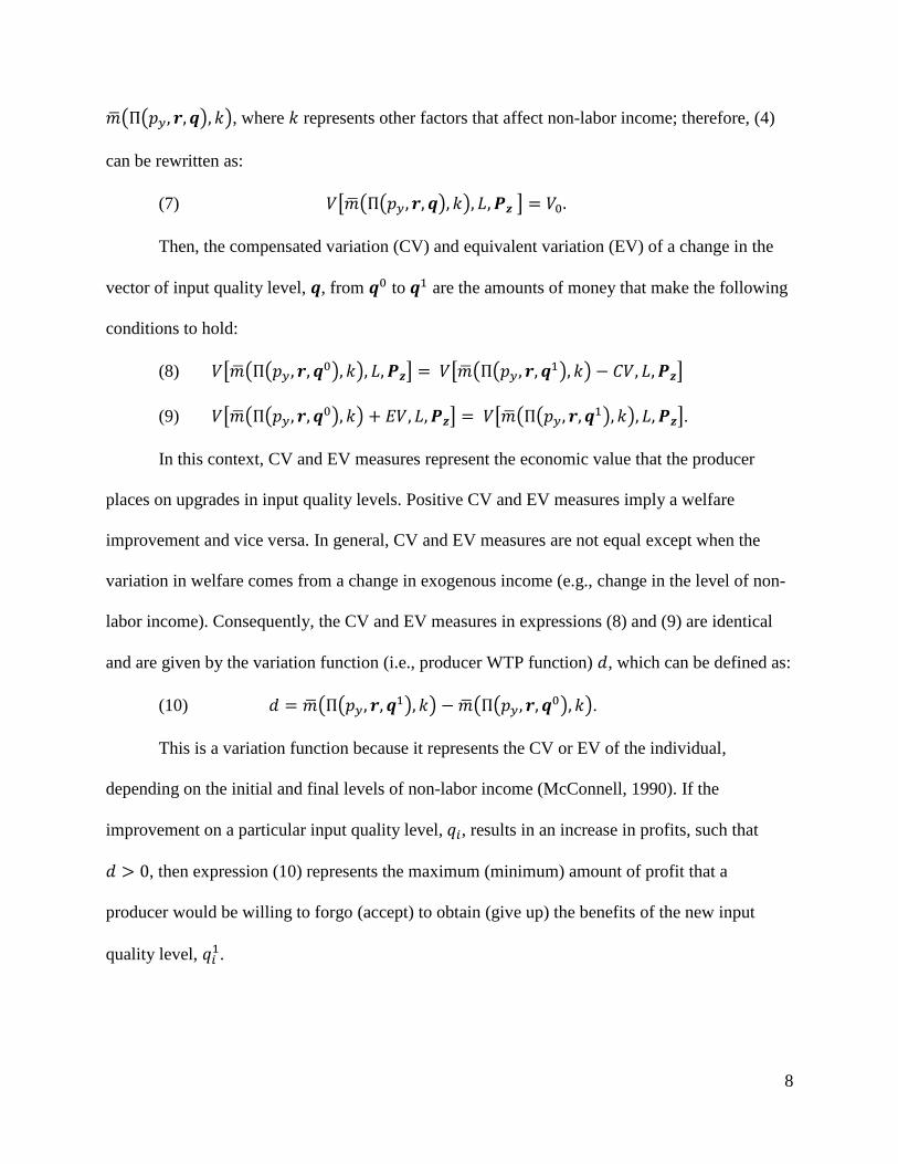
( ( ) ), where represents other factors that affect non-labor income; therefore, (4)

can be rewritten as:

(7) [ ( ( ) ) ]

Then, the compensated variation (CV) and equivalent variation (EV) of a change in the

vector of input quality level, , from to are the amounts of money that make the following

conditions to hold:

(8) [ ( ( ) ) ] [ ( (

) ) ]

(9) [ ( ( ) ) ] [ ( (

) ) ].

In this context, CV and EV measures represent the economic value that the producer

places on upgrades in input quality levels. Positive CV and EV measures imply a welfare

improvement and vice versa. In general, CV and EV measures are not equal except when the

variation in welfare comes from a change in exogenous income (e.g., change in the level of non-

labor income). Consequently, the CV and EV measures in expressions (8) and (9) are identical

and are given by the variation function (i.e., producer WTP function) , which can be defined as:

(10) ( ( ) ) ( (

) ).

This is a variation function because it represents the CV or EV of the individual,

depending on the initial and final levels of non-labor income (McConnell, 1990). If the

improvement on a particular input quality level, , results in an increase in profits, such that

, then expression (10) represents the maximum (minimum) amount of profit that a

producer would be willing to forgo (accept) to obtain (give up) the benefits of the new input

quality level, .

9

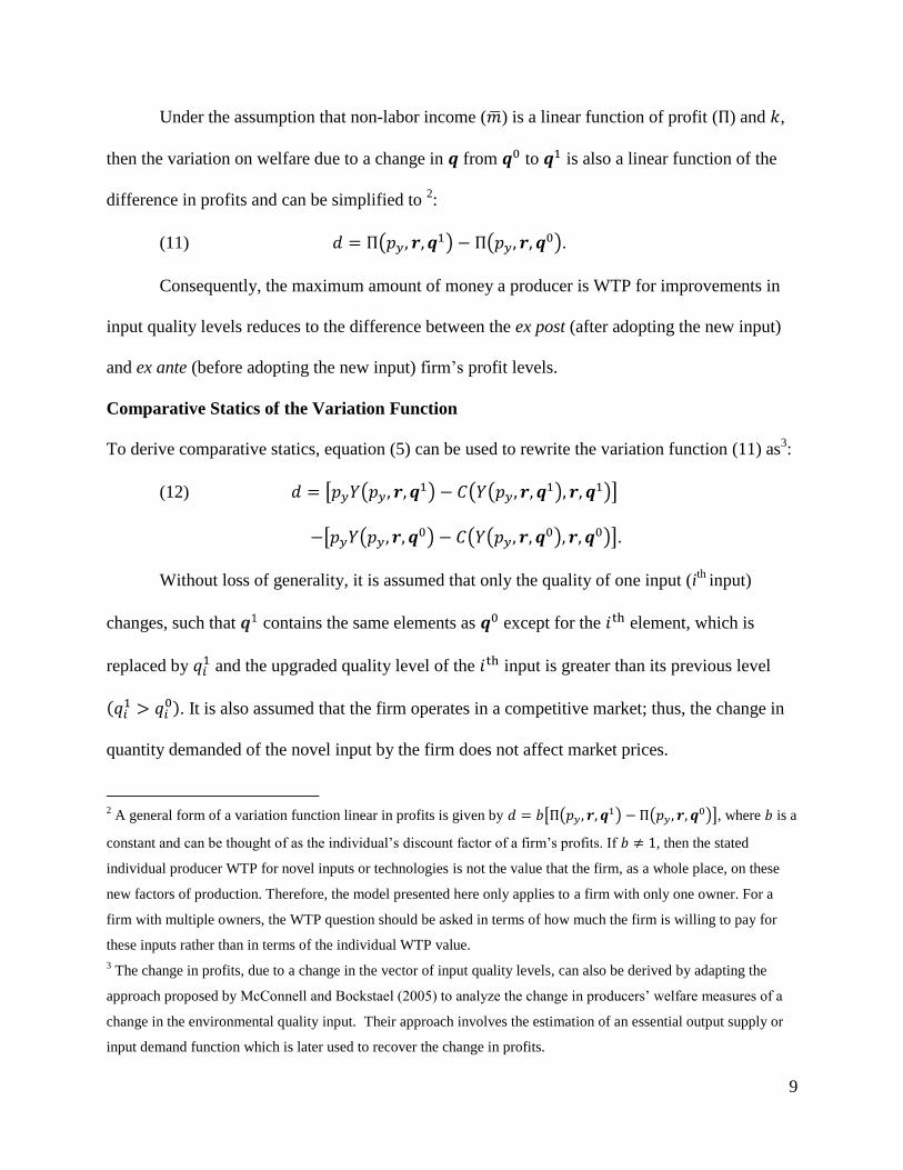
Under the assumption that non-labor income ( ) is a linear function of profit ( ) and ,

then the variation on welfare due to a change in from to is also a linear function of the

difference in profits and can be simplified to 2:

(11) ( ) (

).

Consequently, the maximum amount of money a producer is WTP for improvements in

input quality levels reduces to the difference between the ex post (after adopting the new input)

and ex ante (before adopting the new input) firm’s profit levels.

Comparative Statics of the Variation Function

To derive comparative statics, equation (5) can be used to rewrite the variation function (11) as3:

(12) [ ( ) ( (

) )]

[ ( ) ( (

) )].

Without loss of generality, it is assumed that only the quality of one input (ith

input)

changes, such that contains the same elements as except for the element, which is

replaced by and the upgraded quality level of the input is greater than its previous level

(

). It is also assumed that the firm operates in a competitive market; thus, the change in

quantity demanded of the novel input by the firm does not affect market prices.

2 A general form of a variation function linear in profits is given by [ (

) ( )], where is a

constant and can be thought of as the individual’s discount factor of a firm’s profits. If , then the stated

individual producer WTP for novel inputs or technologies is not the value that the firm, as a whole place, on these

new factors of production. Therefore, the model presented here only applies to a firm with only one owner. For a

firm with multiple owners, the WTP question should be asked in terms of how much the firm is willing to pay for

these inputs rather than in terms of the individual WTP value.

3 The change in profits, due to a change in the vector of input quality levels, can also be derived by adapting the

approach proposed by McConnell and Bockstael (2005) to analyze the change in producers’ welfare measures of a

change in the environmental quality input. Their approach involves the estimation of an essential output supply or

input demand function which is later used to recover the change in profits.

10

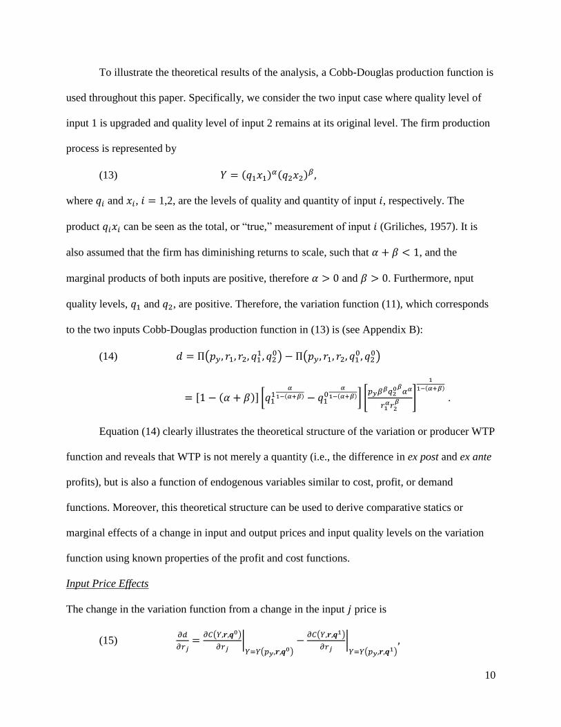
To illustrate the theoretical results of the analysis, a Cobb-Douglas production function is

used throughout this paper. Specifically, we consider the two input case where quality level of

input 1 is upgraded and quality level of input 2 remains at its original level. The firm production

process is represented by

(13) ( ) ( )

where and , 1,2, are the levels of quality and quantity of input , respectively. The

product can be seen as the total, or “true,” measurement of input (Griliches, 1957). It is

also assumed that the firm has diminishing returns to scale, such that , and the

marginal products of both inputs are positive, therefore and . Furthermore, nput

quality levels, and , are positive. Therefore, the variation function (11), which corresponds

to the two inputs Cobb-Douglas production function in (13) is (see Appendix B):

(14) (

) (

)

[ ( )] [

( )

( )] [

]

( )

.

Equation (14) clearly illustrates the theoretical structure of the variation or producer WTP

function and reveals that WTP is not merely a quantity (i.e., the difference in ex post and ex ante

profits), but is also a function of endogenous variables similar to cost, profit, or demand

functions. Moreover, this theoretical structure can be used to derive comparative statics or

marginal effects of a change in input and output prices and input quality levels on the variation

function using known properties of the profit and cost functions.

Input Price Effects

The change in the variation function from a change in the input price is

(15)

( )

| (

)

( )

| (

)

11

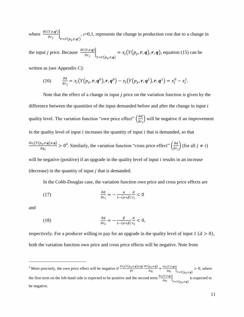
where ( )

| (

)

, =0,1, represents the change in production cost due to a change in

the input price. Because ( )

| ( )

( ( ) ), equation (15) can be

written as (see Appendix C):

(16)

( (

) ) ( ( ) )

Note that the effect of a change in input price on the variation function is given by the

difference between the quantities of the input demanded before and after the change in input

quality level. The variation function “own price effect” (

) will be negative if an improvement

in the quality level of input increases the quantity of input that is demanded, so that

( ( ) )

4

. Similarly, the variation function “cross price effect” (

) (for all )

will be negative (positive) if an upgrade in the quality level of input results in an increase

(decrease) in the quantity of input that is demanded.

In the Cobb-Douglas case, the variation function own price and cross price effects are

(17)

( )

and

(18)

( )

,

respectively. For a producer willing to pay for an upgrade in the quality level of input 1 ( ),

both the variation function own price and cross price effects will be negative. Note from

4 More precisely, the own price effect will be negative if

( ( ) )

( )

( )

| ( )

, where

the first term on the left-hand side is expected to be positive and the second term ( )

| ( )

is expected to

be negative.

12

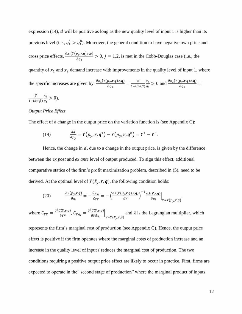
expression (14), will be positive as long as the new quality level of input 1 is higher than its

previous level (i.e.,

). Moreover, the general condition to have negative own price and

cross price effects, ( ( ) )

, , is met in the Cobb-Douglas case (i.e., the

quantity of and demand increase with improvements in the quality level of input 1, where

the specific increases are given by ( ( ) )

( )

and

( ( ) )

( )

).

Output Price Effect

The effect of a change in the output price on the variation function is (see Appendix C):

(19)

(

) ( )

Hence, the change in , due to a change in the output price, is given by the difference

between the ex post and ex ante level of output produced. To sign this effect, additional

comparative statics of the firm’s profit maximization problem, described in (5), need to be

derived. At the optimal level of ( ), the following condition holds:

(20) ( )

(

( ( ) )

) ( )

| ( )

,

where ( )

,

( )

| ( )

and is the Lagrangian multiplier, which

represents the firm’s marginal cost of production (see Appendix C). Hence, the output price

effect is positive if the firm operates where the marginal costs of production increase and an

increase in the quality level of input reduces the marginal cost of production. The two

conditions requiring a positive output price effect are likely to occur in practice. First, firms are

expected to operate in the “second stage of production” where the marginal product of inputs

13

decreases with each extra unit of input; therefore, the marginal cost to produce each additional

unit of output increases. Second, at given input prices and output levels, the use of more efficient

inputs (e.g., inputs with higher quality levels) is expected to reduce costs that are incurred in

producing each additional unit of output.

In the Cobb-Douglas case, the output price effect is positive and is given by

(21)

( )

.

Once again, the output price effect will be positive if . Additionally, the general properties,

identified in expression (20), are ( ( ) )

( )

( )

and

( )

| ( )

( )

, where is positive because the cost function is non-decreasing in output (see

Appendix B).

Input Quality Effects

The effect of a change in the initial quality level of input on the variation function is

(22)

( )

|

( )

.

Note that expression (22) represents the change in the firm’s original production cost

because of a change in the initial quality level of input . The firm’s cost minimization problem

described in (6) allows us to rewrite (22) as

(23)

( (

) ) ,

where

( )

|

( ( ) )

can also be seen as the marginal product of

evaluated at the original input quality levels (see Appendix C). Note that the initial input quality

effect will be negative if the firm operates where both the marginal costs of production and the

14

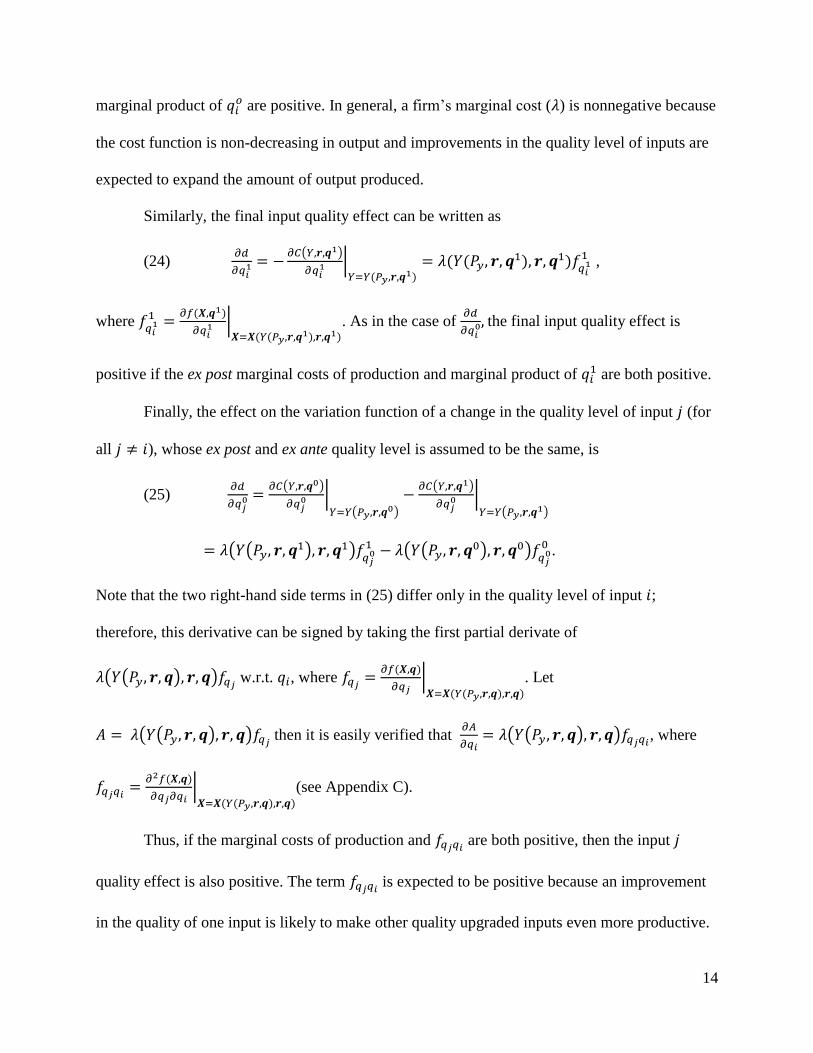
marginal product of are positive. In general, a firm’s marginal cost ( ) is nonnegative because

the cost function is non-decreasing in output and improvements in the quality level of inputs are

expected to expand the amount of output produced.

Similarly, the final input quality effect can be written as

(24)

( )

|

( )

( ( ) )

,

where

( )

|

( ( ) )

. As in the case of

the final input quality effect is

positive if the ex post marginal costs of production and marginal product of are both positive.

Finally, the effect on the variation function of a change in the quality level of input (for

all ), whose ex post and ex ante quality level is assumed to be the same, is

(25)

( )

|

( )

( )

|

( )

( ( ) )

( (

) ) .

Note that the two right-hand side terms in (25) differ only in the quality level of input ;

therefore, this derivative can be signed by taking the first partial derivate of

( ( ) ) w.r.t. , where ( )

| ( ( ) )

. Let

( ( ) ) then it is easily verified that

( ( ) ) , where

( )

| ( ( ) )

(see Appendix C).

Thus, if the marginal costs of production and are both positive, then the input

quality effect is also positive. The term is expected to be positive because an improvement

in the quality of one input is likely to make other quality upgraded inputs even more productive.

15

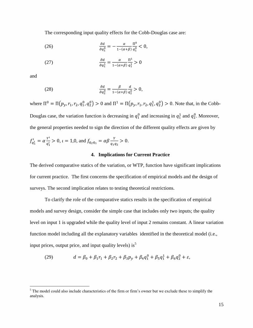
The corresponding input quality effects for the Cobb-Douglas case are:

(26)

( )

,

(27)

( )

and

(28)

( )

,

where (

) and (

) . Note that, in the Cobb-

Douglas case, the variation function is decreasing in and increasing in

and . Moreover,

the general properties needed to sign the direction of the different quality effects are given by

, , and

.

4. Implications for Current Practice

The derived comparative statics of the variation, or WTP, function have significant implications

for current practice. The first concerns the specification of empirical models and the design of

surveys. The second implication relates to testing theoretical restrictions.

To clarify the role of the comparative statics results in the specification of empirical

models and survey design, consider the simple case that includes only two inputs; the quality

level on input 1 is upgraded while the quality level of input 2 remains constant. A linear variation

function model including all the explanatory variables identified in the theoretical model (i.e.,

input prices, output price, and input quality levels) is5

(29)

5 The model could also include characteristics of the firm or firm’s owner but we exclude these to simplify the

analysis.

16

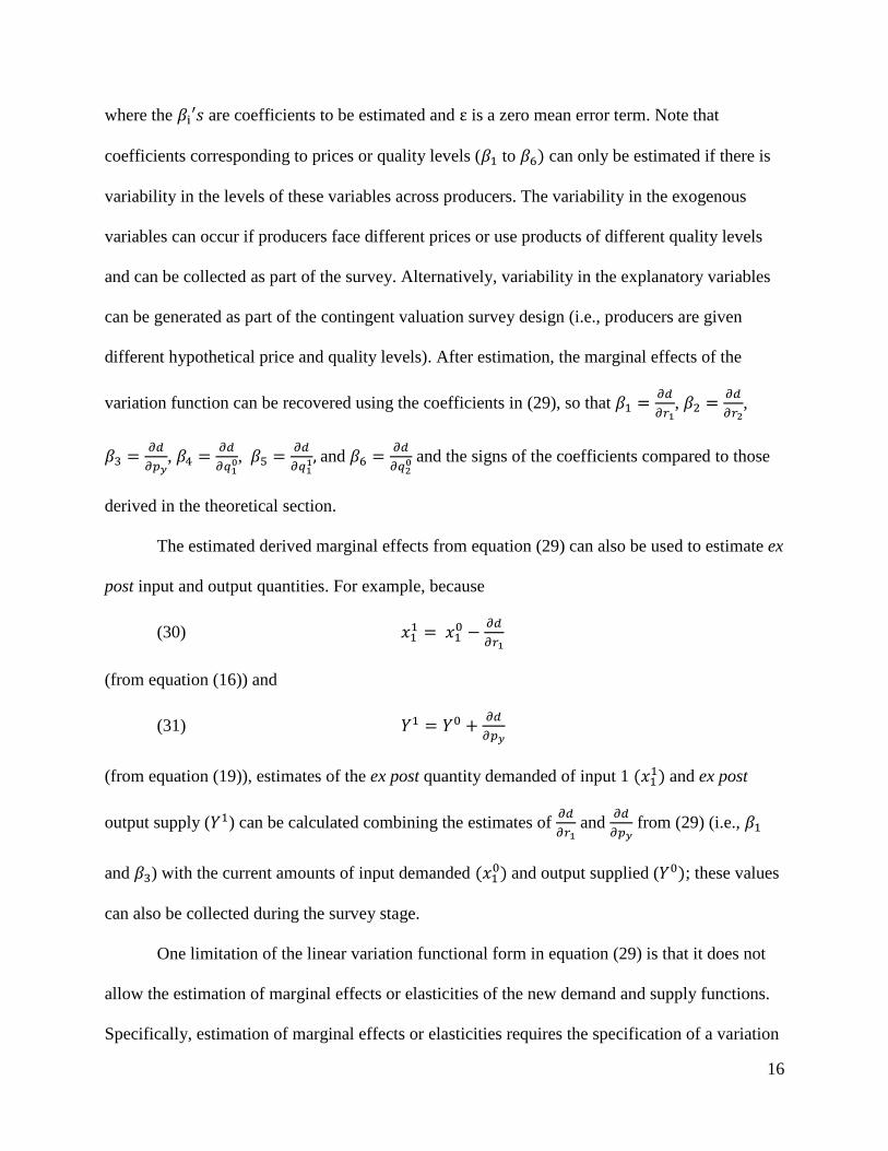
where the are coefficients to be estimated and is a zero mean error term. Note that

coefficients corresponding to prices or quality levels ( to ) can only be estimated if there is

variability in the levels of these variables across producers. The variability in the exogenous

variables can occur if producers face different prices or use products of different quality levels

and can be collected as part of the survey. Alternatively, variability in the explanatory variables

can be generated as part of the contingent valuation survey design (i.e., producers are given

different hypothetical price and quality levels). After estimation, the marginal effects of the

variation function can be recovered using the coefficients in (29), so that

,

,

,

,

and

and the signs of the coefficients compared to those

derived in the theoretical section.

The estimated derived marginal effects from equation (29) can also be used to estimate ex

post input and output quantities. For example, because

(30)

(from equation (16)) and

(31)

(from equation (19)), estimates of the ex post quantity demanded of input 1 ( ) and ex post

output supply ( ) can be calculated combining the estimates of

and

from (29) (i.e.,

and ) with the current amounts of input demanded ( ) and output supplied ( ); these values

can also be collected during the survey stage.

One limitation of the linear variation functional form in equation (29) is that it does not

allow the estimation of marginal effects or elasticities of the new demand and supply functions.

Specifically, estimation of marginal effects or elasticities requires the specification of a variation

17

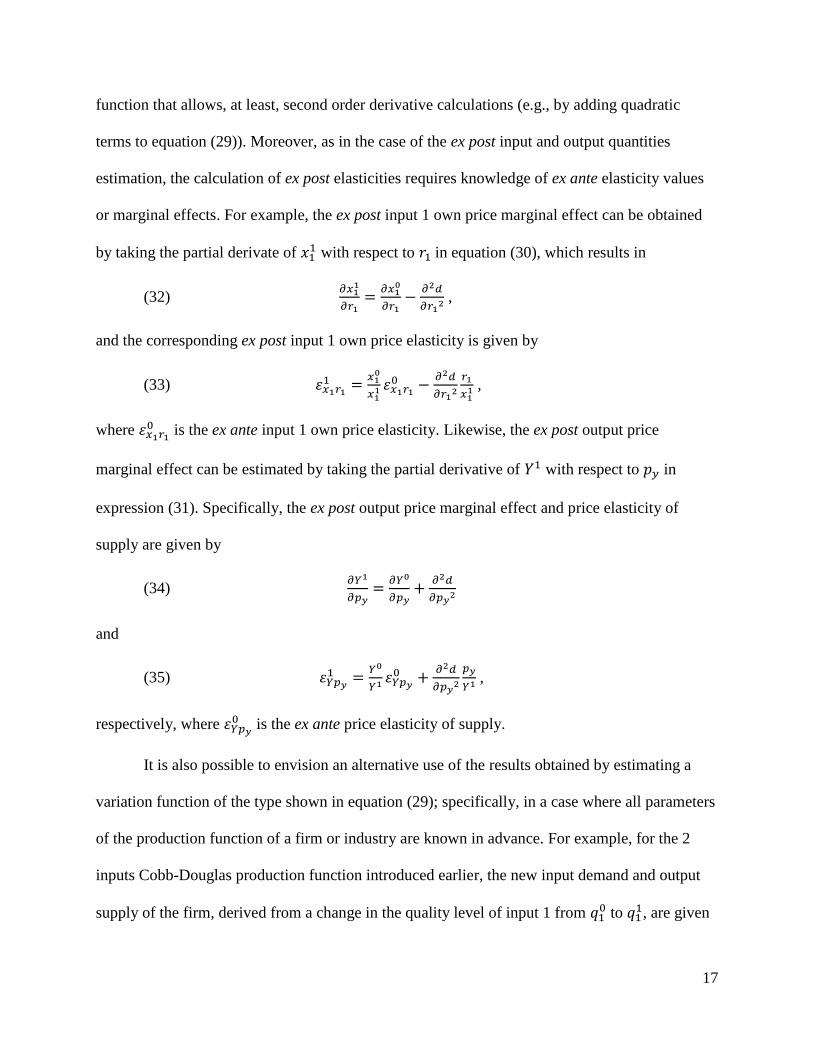
function that allows, at least, second order derivative calculations (e.g., by adding quadratic

terms to equation (29)). Moreover, as in the case of the ex post input and output quantities

estimation, the calculation of ex post elasticities requires knowledge of ex ante elasticity values

or marginal effects. For example, the ex post input 1 own price marginal effect can be obtained

by taking the partial derivate of with respect to in equation (30), which results in

(32)

,

and the corresponding ex post input 1 own price elasticity is given by

(33)

,

where is the ex ante input 1 own price elasticity. Likewise, the ex post output price

marginal effect can be estimated by taking the partial derivative of with respect to in

expression (31). Specifically, the ex post output price marginal effect and price elasticity of

supply are given by

(34)

and

(35)

,

respectively, where is the ex ante price elasticity of supply.

It is also possible to envision an alternative use of the results obtained by estimating a

variation function of the type shown in equation (29); specifically, in a case where all parameters

of the production function of a firm or industry are known in advance. For example, for the 2

inputs Cobb-Douglas production function introduced earlier, the new input demand and output

supply of the firm, derived from a change in the quality level of input 1 from to

, are given

18

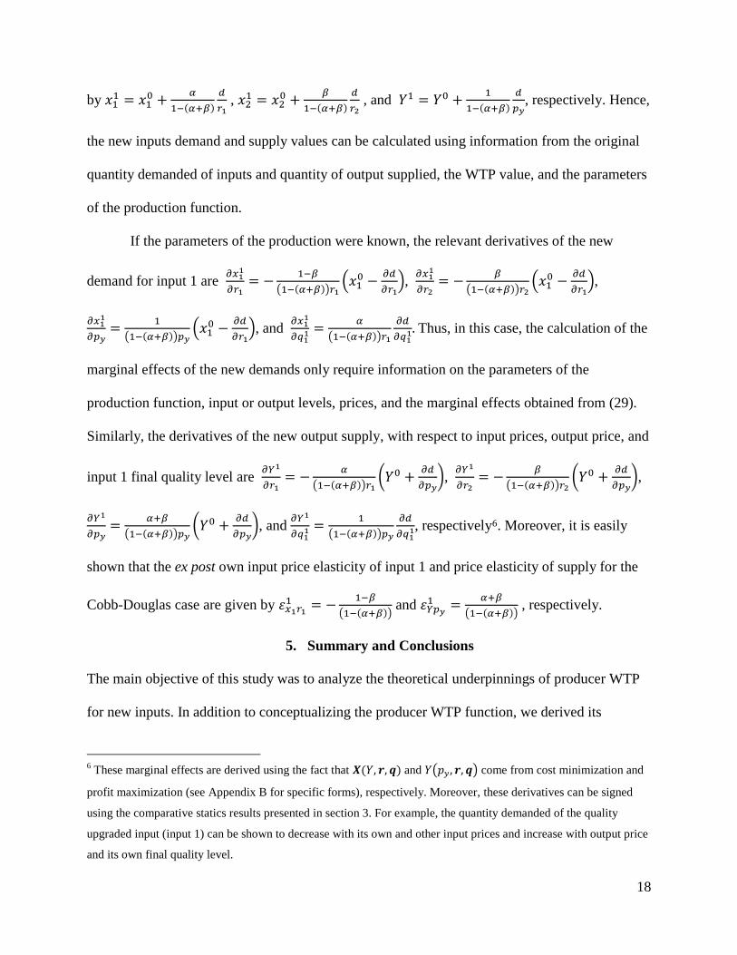
by

( )

,

( )

, and

( )

, respectively. Hence,

the new inputs demand and supply values can be calculated using information from the original

quantity demanded of inputs and quantity of output supplied, the WTP value, and the parameters

of the production function.

If the parameters of the production were known, the relevant derivatives of the new

demand for input 1 are

( ( )) (

),

( ( )) (

),

( ( )) (

), and

( ( ))

Thus, in this case, the calculation of the

marginal effects of the new demands only require information on the parameters of the

production function, input or output levels, prices, and the marginal effects obtained from (29).

Similarly, the derivatives of the new output supply, with respect to input prices, output price, and

input 1 final quality level are

( ( )) (

),

( ( )) (

),

( ( )) (

), and

( ( ))

, respectively6. Moreover, it is easily

shown that the ex post own input price elasticity of input 1 and price elasticity of supply for the

Cobb-Douglas case are given by

( ( )) and

( ( )) , respectively.

5. Summary and Conclusions

The main objective of this study was to analyze the theoretical underpinnings of producer WTP

for new inputs. In addition to conceptualizing the producer WTP function, we derived its

6 These marginal effects are derived using the fact that ( ) and ( ) come from cost minimization and

profit maximization (see Appendix B for specific forms), respectively. Moreover, these derivatives can be signed

using the comparative statics results presented in section 3. For example, the quantity demanded of the quality

upgraded input (input 1) can be shown to decrease with its own and other input prices and increase with output price

and its own final quality level.

19

comparative statics and showed how these properties can be used to recovery quantity demanded

or supplied and, in some cases, price elasticities. We also discussed implications of this

relationship to specify empirical WTP models and survey design.

The WTP model presented was developed within the context of neoclassical theories of

utility and profit maximization. More specifically, the variation function, or producers’ WTP, for

novel inputs or technologies is derived using an individual indirect utility function in

combination with the firm’s profit function. This theoretical model is developed in a context

where the production function ( ) has, as arguments, a vector of input quantities and a vector

of input quality levels . The level of is fixed exogenously, thus the profit and cost functions

are also conditional on . The analysis considers an improvement on a particular input quality

level, .

The theoretical results imply that the maximum amount of money that a producer is WTP

for a new production factor is equal to the difference between the ex post and ex ante firm’s

profit levels. Moreover, the results suggest that the producers’ WTP is a function of output and

input prices and input ex ante and ex post quality levels. Comparative statics results show that

producers’ WTP is a decreasing function of upgraded input price, its initial quality level, and an

increasing function of output price and final quality level.

Use of the structure required by profit and utility maximization is also helpful in

empirical practice. Here, we demonstrated the use of comparative statics results to estimate input

demanded, output supplied, and price elasticities after the change in the input quality. However,

estimation of these values is dependent upon the empirical model used and data availability.

Thus, the results of this study should be of considerable use in specifying empirical WTP models

and survey design.

20

6. References

Cameron, T.A. 1988. A new paradigm for valuing non-market goods using referendum data.

Journal of Environmental Economics and Management 15: 355-379.

Carpio, C.E., and Isengildina-Massa, O. 2009. Consumer Willingness to Pay for Locally Grown

Products: The Case of South Carolina. Agribusiness 25 (3): 412-426.

Carson, R. T., Wright, J. L., Carson, N. J., Alberini, A., Flores, N. E. 1995. A Bibliography of

Contingent Valuation Studies and Papers. Natural Resource Damage Assessment, Inc.,

La Jolla, CA.

Carson, R.T., Hanemann, W.M. 2005. Contingent valuation. In Handbook on Environmental

Economics, Vol 2. Edited by Mäler, K.G., Vincent, J.R. North-Holland, Amsterdam.

Banfi, S., Farsi, M., Filippini, M., Jakob, M. 2008. Willingness to pay for energy-saving

measures in residential buildings, Energy Economics 30: 503-506.

Boyle, K.J. 2003. Contingent valuation in practice. In A primer on nonmarket valuation. Edited

by Champ, P.A., Boyle, K.J., Brown, T.C. Kluwer Academic Publishers, Dordrecht.

Breffle, W.S., Morey, E.R., Lodder, T.S. 1998. Using contingent valuation to estimate a

neighbourhood's willingness to pay to preserve undeveloped urban land. Urban Studies

35(4): 715–727.

Budak, D.B., Budak, F., and Kaçira, Ö.Ö. 2010. Livestock producers’ needs and willingness to

pay for extension services in Adana province of Turkey. African Journal of Agricultural

Research 5(11):1187-1190.

Davis, R. K. 1963. The value of outdoor recreation: an economic study of the Maine woods.

Ph.D. dissertation. Harvard University.

21

Diener, A., O’Brien, B., Gafni, A. 1998. Health care contingent valuation studies: a review and

classification of the literature. Health Economics 7: 313–326.

Griliches, W. 1957. Specification bias in estimates of production functions. Journal of Farm

Economics 39, 8-20.

Hanemann, W.M. 1984. Welfare evaluations in contingent valuation experiments with discrete

responses. American Journal of Agricultural Economics 66, 322-314.

Hudson, D., Hite, H. 2003. Producer willingness to pay for precision application technology:

implications for government and the technology industry. Canadian Journal of

Agricultural Economics 51, 39–53.

Kenkel, P.L., Norris, P.E. 1995. Agricultural Producers' Willingness to Pay for Real-Time

Mesoscale Weather Information. Journal of Agricultural and Resource Economics 20(2):

356-372

Krupnick, A., Alberini, A., Cropper, M., Simon, N., O’Brien, B., Goeree, R., Heintzelman, M.

2002. Age, health and the willingness to pay for mortality risk reductions: a contingent

valuation study of Ontario residents, Journal of Risk and Uncertainty 24(2):161–186.

Lipscomb, C. 2011. Using contingent valuation to measure property value impacts. Journal of

Property Investment and Finance 29: 448-459.

Lusk, J.L. 2003. Effects of Cheap Talk on Consumer Willingness-to-Pay for Golden Rice.

American Journal of Agricultural Economics 85(4): 840-856.

Lusk, J.L., Hudson, D. 2004. Willingness-to-Pay estimates and their relevance to agribusiness

decision making. Review of Agricultural Economics 26(2): 152–169.

McConnell, K.E. 1990. Models for referendum data: the structure of discrete choice models for

contingent valuation. Journal of Environmental Economics and Management 18: 19-34.

22

McConnell, K.E., Bockstael, N.B. 2005. Valuing the environment as a factor of production. In

Handbook on Environmental Economics, Vol 2. Edited by Mäler, K.G., Vincent, J.R.

North-Holland, Amsterdam.

Patrick, F.G. 1988. Mallee wheat farmers’ demand for crop and rainfall insurance. Australian

Journal of Agricultural Economics 32(1): 37–49.

Thompson, E., Berger, M., Blomquist, G., Allen, S. 2002. Valuing the arts: a contingent

valuation approach. Journal of Cultural Economics 26: 87–113.

Whitehead, J.C. 1995. Willingness to pay for quality improvements: comparative statics and

interpretation of contingent valuation results. Land Economics 71(2): 207-215.

Whitehead, J.C., Hoban, T.J., Clifford, W.B. 2001. Willingness to pay for agricultural research

and extension programs. Journal of Agricultural and Applied Economics 33(1): 91-101.

Zapata, S.D., Benavides, H.M., Carpio, C.E., and Willis, D.B. 2012. The Economic Value of

Basin Protection to Improve the Quality and Reliability of Potable Water Supply: The

Case of Loja, Ecuador. Water Policy 14: 1-13.

23

7. Appendices

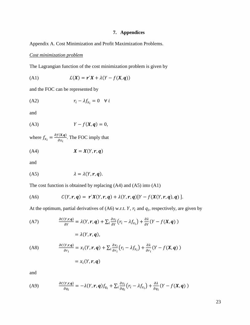
Appendix A. Cost Minimization and Profit Maximization Problems.

Cost minimization problem

The Lagrangian function of the cost minimization problem is given by

(A1) ( ) ( ( ))

and the FOC can be represented by

(A2)

and

(A3) ( ) ,

where ( )

. The FOC imply that

(A4) ( )

and

(A5) ( ).

The cost function is obtained by replacing (A4) and (A5) into (A1)

(A6) ( ) ( ) ( )[ ( ( ) ) ].

At the optimum, partial derivatives of (A6) w.r.t. , and , respectively, are given by

(A7) ( )

( ) ∑

( )

( ( ) )

( ),

(A8) ( )

( ) ∑

( )

( ( ) )

( )

and

(A9) ( )

( ) ∑

( )

( ( ) )

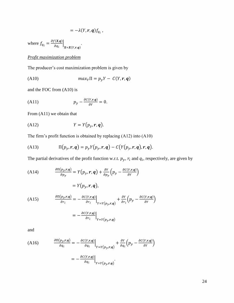
24

( ) ,

where ( )

| ( )

.

Profit maximization problem

The producer’s cost maximization problem is given by

(A10) ( )

and the FOC from (A10) is

(A11) ( )

.

From (A11) we obtain that

(A12) ( ).

The firm’s profit function is obtained by replacing (A12) into (A10)

(A13) ( ) ( ) ( ( ) ).

The partial derivatives of the profit function w.r.t. , and , respectively, are given by

(A14) ( )

( )

(

( )

)

( ),

(A15) ( )

( )

| ( )

(

( )

)

( )

| ( )

and

(A16) ( )

( )

| ( )

(

( )

)

( )

| ( )

.

25

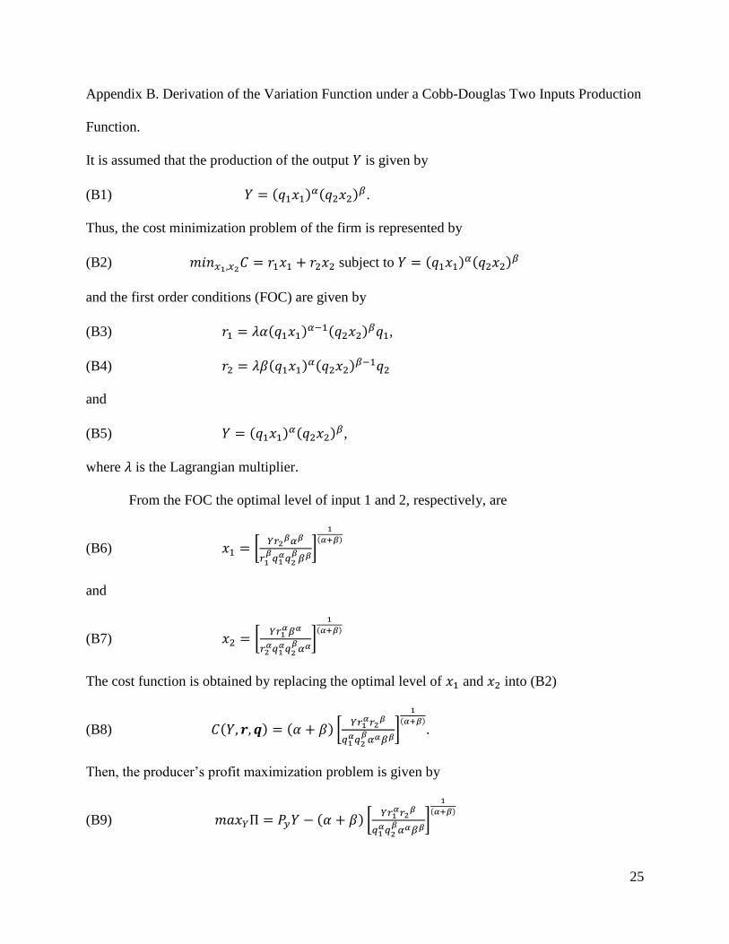
Appendix B. Derivation of the Variation Function under a Cobb-Douglas Two Inputs Production

Function.

It is assumed that the production of the output is given by

(B1) ( ) ( )

.

Thus, the cost minimization problem of the firm is represented by

(B2) subject to ( ) ( )

and the first order conditions (FOC) are given by

(B3) ( ) ( )

,

(B4) ( ) ( )

and

(B5) ( ) ( )

,

where is the Lagrangian multiplier.

From the FOC the optimal level of input 1 and 2, respectively, are

(B6) [

]

( )

and

(B7) [

]

( )

The cost function is obtained by replacing the optimal level of and into (B2)

(B8) ( ) ( ) [

]

( )

.

Then, the producer’s profit maximization problem is given by

(B9) ( ) [

]

( )

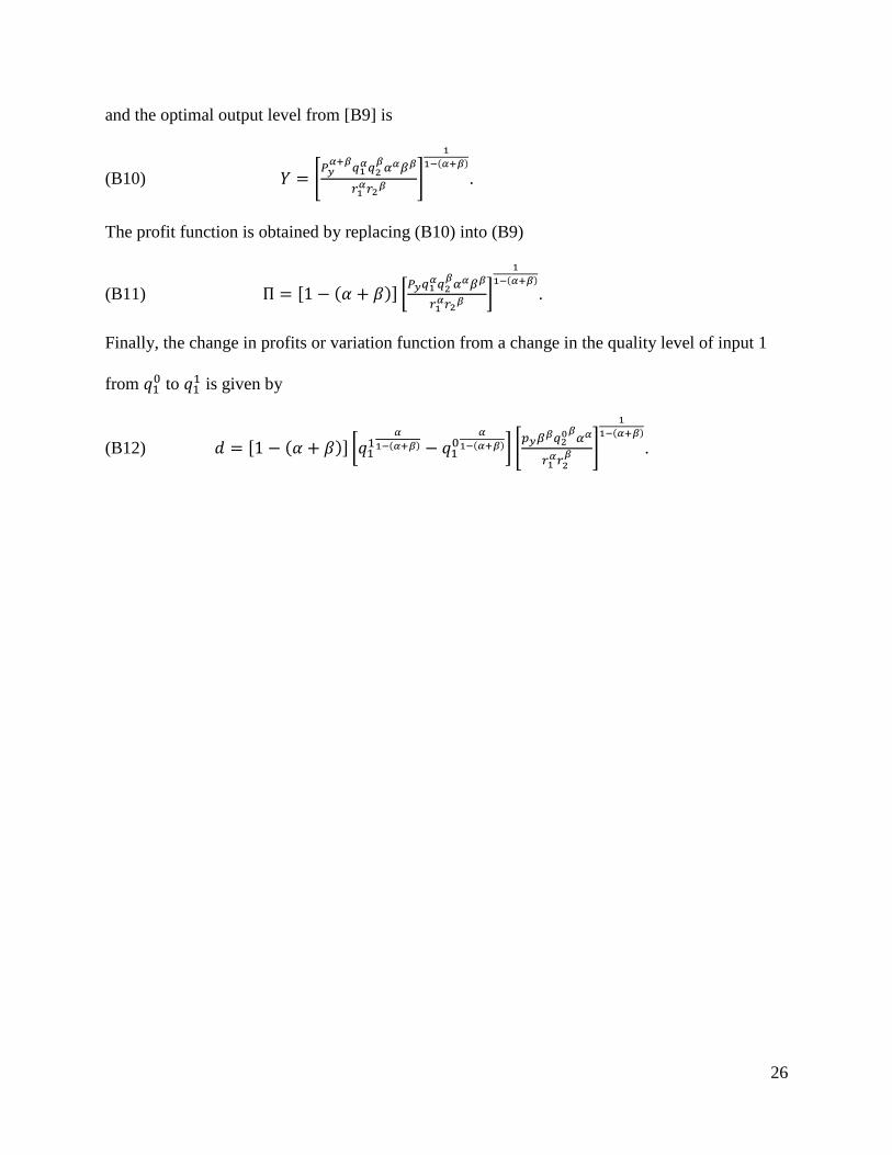
26

and the optimal output level from [B9] is

(B10) [

]

( )

.

The profit function is obtained by replacing (B10) into (B9)

(B11) [ ( )] [

]

( )

.

Finally, the change in profits or variation function from a change in the quality level of input 1

from to

is given by

(B12) [ ( )] [

( )

( )] [

]

( )

.

27

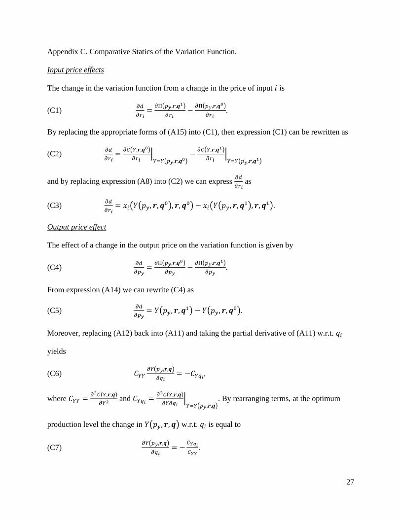
Appendix C. Comparative Statics of the Variation Function.

Input price effects

The change in the variation function from a change in the price of input is

(C1)

(

)

(

)

.

By replacing the appropriate forms of (A15) into (C1), then expression (C1) can be rewritten as

(C2)

( )

| (

) ( )

| (

)

and by replacing expression (A8) into (C2) we can express

as

(C3)

( (

) ) ( ( ) ).

Output price effect

The effect of a change in the output price on the variation function is given by

(C4)

(

)

(

)

.

From expression (A14) we can rewrite (C4) as

(C5)

(

) ( ).

Moreover, replacing (A12) back into (A11) and taking the partial derivative of (A11) w.r.t.

yields

(C6) ( )

,

where ( )

and

( )

| ( )

. By rearranging terms, at the optimum

production level the change in ( ) w.r.t. is equal to

(C7) ( )

.

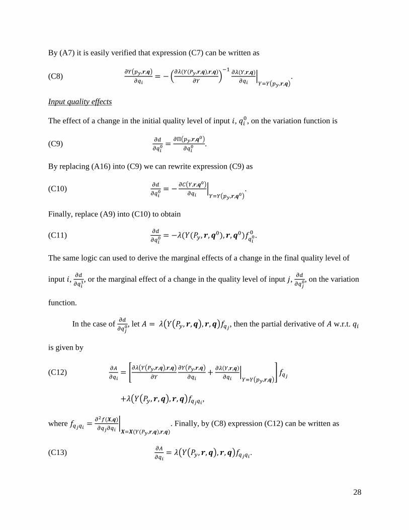
28

By (A7) it is easily verified that expression (C7) can be written as

(C8) ( )

(

( ( ) )

) ( )

| ( )

.

Input quality effects

The effect of a change in the initial quality level of input , , on the variation function is

(C9)

( )

.

By replacing (A16) into (C9) we can rewrite expression (C9) as

(C10)

( )

| (

).

Finally, replace (A9) into (C10) to obtain

(C11)

( (

) ) .

The same logic can used to derive the marginal effects of a change in the final quality level of

input ,

, or the marginal effect of a change in the quality level of input ,

, on the variation

function.

In the case of

, let ( ( ) ) , then the partial derivative of w.r.t.

is given by

(C12)

[

( ( ) )

( )

( )

| ( )

]

( ( ) ) ,

where ( )

| ( ( ) )

. Finally, by (C8) expression (C12) can be written as

(C13)

( ( ) ) .