the theory of consumer choice - wordpress.com · 2015-12-25 · the theory of consumer choice ......

The Theory of

Consumer Choice

The theory of consumer choice

addresses the following questions:

Do all demand curves slope

downward?

How do wages affect labor supply?

How do interest rates affect household

saving?

Do the poor prefer to receive cash or

in-kind transfers?

The Budget Constraint

The budget constraint depicts the

consumption “bundles” that a

consumer can afford.

People consume less than they desire because

their spending is constrained, or limited, by

their income.

The Budget Constraint

It shows the various combinations of

goods the consumer can afford given

his or her income and the prices of

the two goods.

The Consumer’s Opportunities

Pints ofPepsi

Number ofPizzas

Spendingon Pepsi

Spendingon Pizza

TotalSpending

0 100 $ 0 $1,000 $1,000

50 90 100 900 1,000

100 80 200 800 1,000

150 70 300 700 1,000

200 60 400 600 1,000

250 50 500 500 1,000

300 40 600 400 1,000

350 30 700 300 1,000

400 20 800 200 1,000

450 10 900 100 1,000

500 0 1,000 0 1,000

The Consumer’s Budget

Constraint

Any point on the budget constraint line

indicates the consumer’s combination or

tradeoff between two goods.

For example, if the consumer buys no

pizzas, he can afford 500 pints of Pepsi

(point B). If he buys no Pepsi, he can

afford 100 pizzas (point A).


Constraint...

Quantityof Pizza

Quantityof Pepsi

0

Consumer’sbudget constraint

500 B

100

A


Constraint

Alternately, the consumer can buy

50 pizzas and 250 pints of Pepsi.


Constraint...

Quantityof Pizza

Quantityof Pepsi

0

250

50 100

500B

C

A



Constraint

The slope of the budget constraint line

equals the relative price of the two goods,

that is, the price of one good compared to

the price of the other.

It measures the rate at which the

consumer will trade one good for the

other.

Preferences:

What the Consumer Wants

A consumer’s preference among

consumption bundles may be

illustrated with indifference curves.

Representing Preferences with

Indifference Curves

An indifference curve shows

bundles of goods that make the

consumer equally happy.

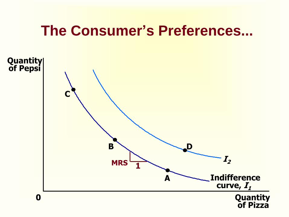
The Consumer’s Preferences...

Quantityof Pizza

Quantityof Pepsi

0

C

B

A Indifferencecurve, I1

D

I2

The consumer is indifferent, or equally

happy, with the combinations shown at

points A, B, and C because they are all on

the same curve.

The Consumer’s Preferences

The Marginal Rate of Substitution

The slope at any point on an indifference

curve is the marginal rate of substitution.

It is the rate at which a consumer is willing to

substitute one good for another.

It is the amount of one good that a consumer

requires as compensation to give up one unit

of the other good.


Quantityof Pizza

Quantityof Pepsi

0

C

B

A

D

Indifferencecurve, I1

I21MRS

Properties of Indifference Curves

Higher indifference curves are

preferred to lower ones.

Indifference curves are downward

sloping.

Indifference curves do not cross.

Indifference curves are bowed

inward.

Property 1: Higher indifference curves are


Consumers usually prefer more of

something to less of it.

Higher indifference curves represent

larger quantities of goods than do

lower indifference curves.



Quantityof Pizza

Quantityof Pepsi

0

C

B

A

D


I2

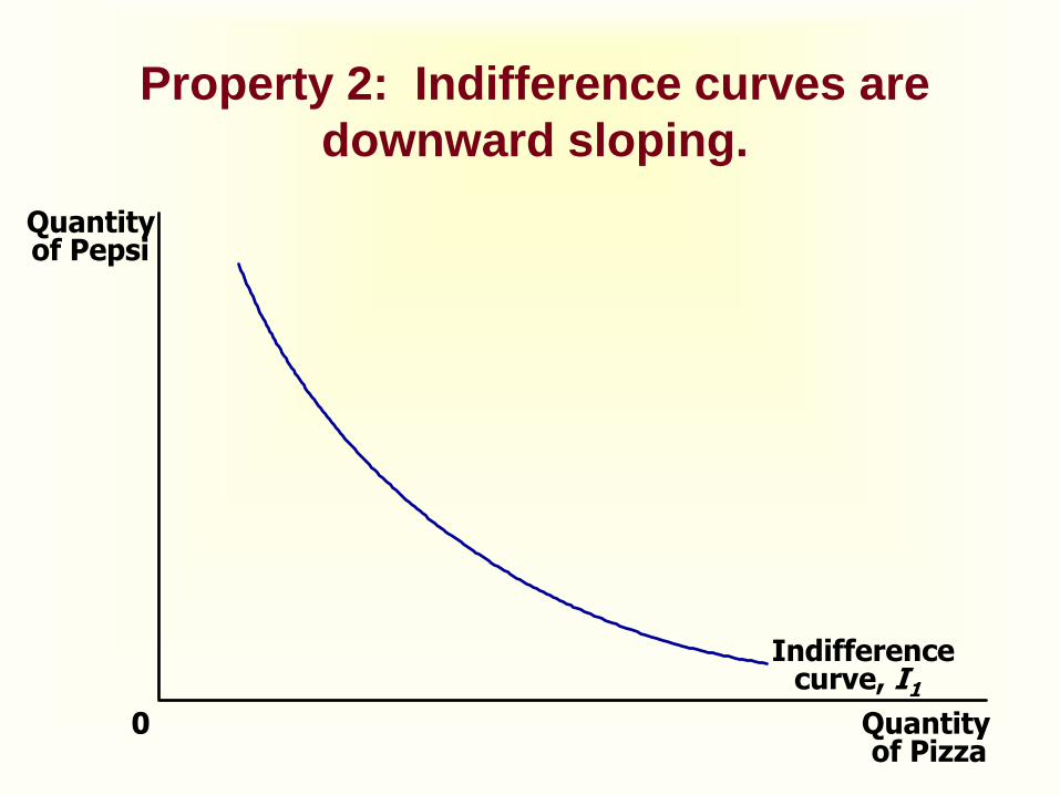
Property 2: Indifference curves are

downward sloping.

A consumer is willing to give up one good

only if he or she gets more of the other

good in order to remain equally happy.

If the quantity of one good is reduced, the

quantity of the other good must increase.

For this reason, most indifference curves

slope downward.


downward sloping.

Quantityof Pizza

Quantityof Pepsi

0


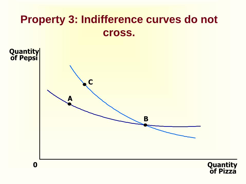
Property 3: Indifference curves do not

cross.

Points A and B should make the


Points B and C should make the


This implies that A and C would make

the consumer equally happy.

But C has more of both goods

compared to A.


cross.

Quantityof Pizza

Quantityof Pepsi

0

C

A

B


bowed inward.

People are more willing to trade away

goods that they have in abundance and

less willing to trade away goods of which

they have little.

These differences in a consumer’s

marginal substitution rates cause his or

her indifference curve to bow inward.

1MRS = 1

8

3

Indifferencecurve

A


bowed inward.

Quantityof Pizza

Quantityof Pepsi

0

14

2

3

7

B

1

MRS = 6

4

6

Two Extreme Examples of

Indifference Curves

Perfect substitutes

Perfect complements

Perfect Substitutes

Two goods with straight-line

indifference curves are perfect

substitutes.

The marginal rate of substitution is a fixed

number.

Perfect Substitutes

Dimes0

Nickels

21

4

2

I1I2

6

3

I3

Perfect Complements

Two goods with right-angle

indifference curves are perfect

complements.

Perfect Complements

Right Shoes0

LeftShoes

75

7

5 I1

I2

Optimization: What the Consumer

Chooses

Consumers want to get the

combination of goods on the highest

possible indifference curve.

However, the consumer must also end

up on or below his budget constraint.

Optimization: What the Consumer

Chooses

Combining the indifference curve and the

budget constraint determines the

consumer’s optimal choice.

Consumer optimum occurs at the point

where the highest indifference curve and

the budget constraint are tangent.

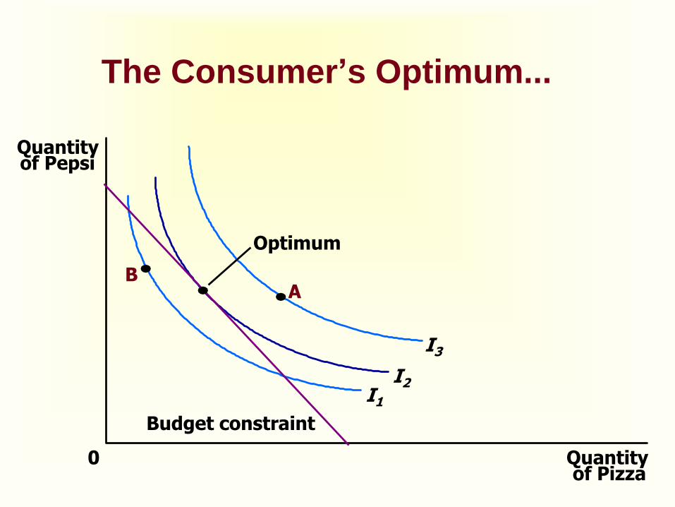
The Consumer’s Optimal Choice

The consumer chooses consumption of

the two goods so that the marginal rate

of substitution equals the relative price.

The Consumer’s Optimal Choice

At the consumer’s optimum, the

consumer’s valuation of the two goods

equals the market’s valuation.

The Consumer’s Optimum...

Quantityof Pizza

Quantityof Pepsi

0

I1

I2

I3

Budget constraint

AB

Optimum

How Changes in Income Affect the

Consumer’s Choices

An increase in income shifts the budget

constraint outward.

The consumer is able to choose a better

combination of goods on a higher

indifference curve.

An Increase in Income...

Quantityof Pizza

Quantityof Pepsi

0

I1

I2

2. …raising pizza consumption…

3. …and Pepsiconsumption.

Initial optimum

New budget constraint

1. An increase in income shifts the budget constraint outward…

Initial budget

constraint

New optimum

Normal versus Inferior Goods

If a consumer buys more of a good

when his or her income rises, the good

is called a normal good.

If a consumer buys less of a good when

his or her income rises, the good is

called an inferior good.


1. When an increase in income shifts the budget constraint outward...

An Inferior Good...

Quantityof Pizza

Quantityof Pepsi

0

Initial optimum

I1

New optimum

I2

2. ... pizza consumption rises, making pizza a normal good...

3. ... but Pepsi consumption falls, making Pepsi an inferior good.

Initial budget

constraint

How Changes in Prices Affect

Consumer Choices

A fall in the price of any good

rotates the budget constraint

outward and changes the slope

of the budget constraint.

A Change in Price...

Quantity of Pizza100

Quantity of Pepsi

1,000

500

0

I1


3. …and raising Pepsiconsumption.

Initial budget constraint

2. …reducing pizza consumption…

1. A fall in the price of Pepsi rotates the budget constraint outward…

New optimum

I2

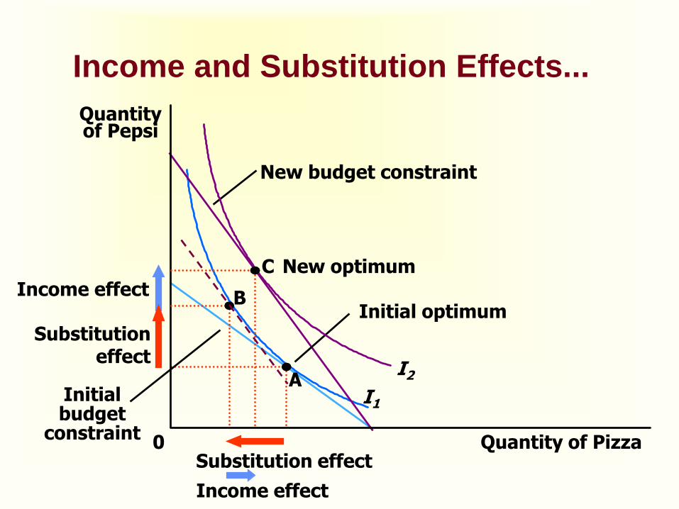
Income and Substitution Effects

A price change has two effects on

consumption.

An income effect

A substitution effect

The Income Effect

The income effect is the change in

consumption that results when a

price change moves the consumer

to a higher or lower indifference

curve.

The Substitution Effect

The substitution effect is the change in

consumption that results when a price

change moves the consumer along an

indifference curve to a point with a

different marginal rate of substitution.

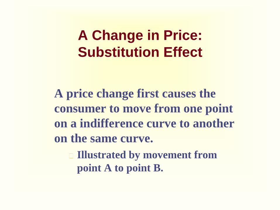
A Change in Price:

Substitution Effect

A price change first causes the

consumer to move from one point

on a indifference curve to another

on the same curve.

Illustrated by movement from

point A to point B.

A Change in Price:

Income Effect

After moving from one point to

another on the same curve, the

consumer will move to another

indifference curve.

Illustrated by movement from

point B to point C.

Income and Substitution Effects...

Quantity of Pizza

Quantityof Pepsi

0

A

Initial optimum

I1


Initial budget

constraint

I2

C New optimumIncome effect

Income effect

Substitution effect

B

Substitution effect

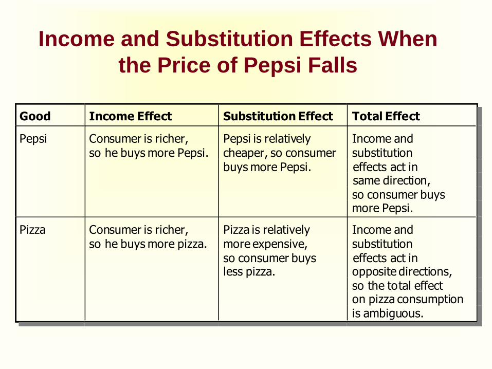
Income and Substitution Effects When

the Price of Pepsi Falls

Good Income Effect Substitution Effect Total Effect

Pepsi Consumer is richer,so he buys more Pepsi.

Pepsi is relativelycheaper, so consumerbuys more Pepsi.

Income andsubstitutioneffects act insame direction,so consumer buys more Pepsi.

Pizza Consumer is richer,so he buys more pizza.

Pizza is relativelymore expensive,so consumer buys less pizza.

Income andsubstitutioneffects act inopposite directions,so the total effecton pizza consumptionis ambiguous.

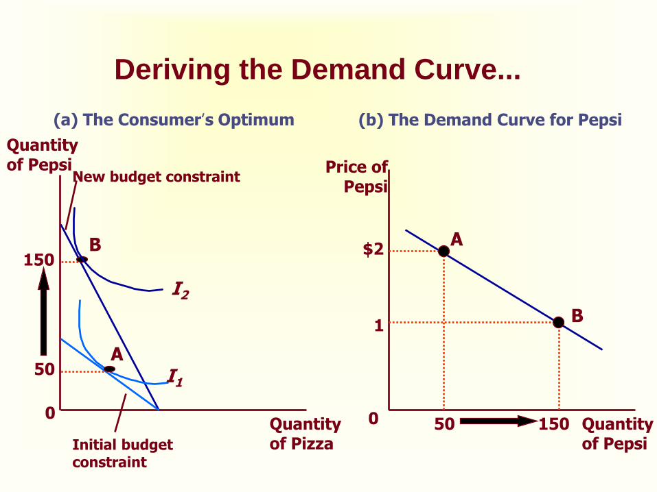
Deriving the Demand Curve

A consumer’s demand curve can be

viewed as a summary of the optimal

decisions that arise from his or her

budget constraint and indifference

curves.

Deriving the Demand Curve...

(a) The Consumer’s Optimum (b) The Demand Curve for Pepsi

I1

I2

A

B



50

150

Quantity of Pizza

Quantity of Pepsi

0 0 Quantity of Pepsi

50 150

1

$2

Price of Pepsi

A

B

Do all demand curves slope

downward?

Demand curves can sometimes slope

upward.

This happens when a consumer buys

more of a good when its price rises.

Giffen Goods

Economists use the term Giffen good to

describe a good that violates the law of

demand.

Giffen goods are inferior goods for which

the income effect dominates the

substitution effect.

They have demand curves that slope

upwards.

Quantityof Meat

A

Quantity ofPotatoes

0

E

C

I2

I1


New budgetconstraint

D

B

Optimum with lowprice of potatoes

Optimum with highprice of potatoes

1. An increase in the price of potatoes rotates the budget...

2...which increases potato consumption if potatoes are a Giffen good.

A Giffen Good...

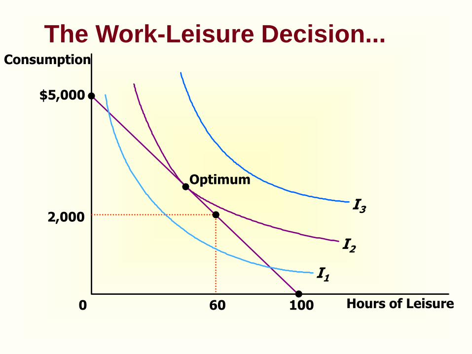
How do wages affect labor

supply?

If the substitution effect is greater than

the income effect for the worker, he or

she works more.

If income effect is greater than the

substitution effect, he or she works

less.

Hours of Leisure0

2,000

$5,000

60

Consumption

100

Optimum

I3

I2

I1

The Work-Leisure Decision...

Hours of LaborSupplied

0

Wage

. . . the labor supply curve slopes upward.

Hours ofLeisure

0

Co

nsu

mp

tio

n

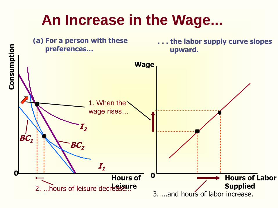
(a) For a person with these preferences…

I2

I1

BC2

BC1

2. …hours of leisure decrease…3. ...and hours of labor increase.

1. When the

wage rises…

An Increase in the Wage...


0

Wage

. . . the labor supply curve slopes backward.

Hours ofLeisure

0

Co

nsu

mp

tio

n

(b) For a person with these preferences…

I2

I1

BC2

BC1

1. When the

wage rises…


2. …hours of leisure increase… 3. ...and hours of labor decrease.

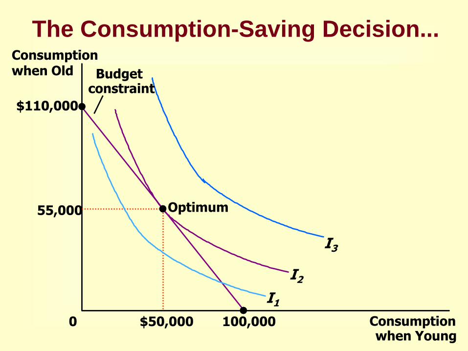
How do interest rates affect

household saving?

If the substitution effect of a higher

interest rate is greater than the income

effect, households save more.

If the income effect of a higher interest

rate is greater than the substitution effect,

households save less.

Consumptionwhen Young

0

55,000

$110,000

$50,000

Consumptionwhen Old

100,000

Optimum

I3

I2

I1

Budgetconstraint

The Consumption-Saving Decision...

An Increase in the Interest Rate...

0

Co

nsu

mp

tio

n

wh

en

Old

1. A higher

interest rate

rotates the

budget constraint

outward...I2

I1

BC2

BC1

2. …resulting in lower consumption when young and, thus, higher saving.

Consumption when Young

Hours ofLeisure

0

I2

I1

BC2

BC1C

on

su

mp

tio

n

wh

en

Old

1. A higher

interest rate

rotates the

budget constraint

outward...

2. …resulting in higher consumption when young and, thus, lower saving.

(a) Higher Interest Rate Raises Saving

(b) Higher Interest Rate Lowers Saving

How do interest rates affect

household saving?

Thus, an increase in the interest

rate could either encourage or

discourage saving.

Do the poor prefer to receive cash

or in-kind transfers?

If an in-kind transfer of a good forces

the recipient to consume more of the

good than he would on his own, then the

recipient prefers the cash transfer.

Do the poor prefer to receive cash

or in-kind transfers?

If the recipient does not consume more

of the good than he would on his own,

then the cash and in-kind transfer have

exactly the same effect on his

consumption and welfare.

Cash Transfer In-Kind Transfer

(a) The Constraint Is Not Binding

NonfoodConsumption

0

$1,000 $1,000

Food

A

B

I2

I1

BC1

BC2(with $1,000 cash)

NonfoodConsumption

0

Food

A

B

I2

I1

BC1

BC2(with $1,000 food stamps)

Cash versus In-Kind Transfers...


(b) The Constraint Is Binding

NonfoodConsumption

0

$1,000 $1,000

Food

A

B

I2I1

BC1


NonfoodConsumption

0

Food

A

BI2

I1

BC1



C

I3

Summary

A consumer’s budget constraint shows

the possible combinations of different

goods he can buy given his income and

the prices of the goods.

The slope of the budget constraint

equals the relative price of the goods.

The consumer’s indifference curves

represent his preferences.

Summary

Points on higher indifference curves are

preferred to points on lower indifference

curves.

The slope of an indifference curve at any

point is the consumer’s marginal rate of

substitution.

The consumer optimizes by choosing the

point on his budget constraint that lies on

the highest indifference curve.

Summary

When the price of a good falls, the impact on

the consumer’s choices can be broken down

into an income effect and a substitution

effect.

The income effect is the change in

consumption that arises because a lower

price makes the consumer better off.

The income effect is reflected by the

movement from a lower to a higher

indifference curve.

Summary

The substitution effect is the change in

consumption that arises because a price

change encourages greater consumption of

the good that has become relatively

cheaper.

The substitution effect is reflected by a

movement along an indifference curve to a

point with a different slope.

Summary

The theory of consumer choice can

explain:

Why demand curves can potentially slope

upward.

How wages affect labor supply.

How interest rates affect household saving.

Whether the poor prefer to receive cash or in-

kind transfers.

Graphical

Review


Constraint...

Quantityof Pizza

Quantityof Pepsi

0


500 B

100

A


Constraint...

Quantityof Pizza

Quantityof Pepsi

0

250

50 100

500B

C

A



Quantityof Pizza

Quantityof Pepsi

0

C

B

A Indifferencecurve, I1

D

I2


Quantityof Pizza

Quantityof Pepsi

0

C

B

A

D


I21MRS



Quantityof Pizza

Quantityof Pepsi

0

C

B

A

D


I2


downward sloping.

Quantityof Pizza

Quantityof Pepsi

0



cross.

Quantityof Pizza

Quantityof Pepsi

0

C

A

B


bowed inward.

1MRS = 1

8

3

Indifferencecurve

A

Quantityof Pizza

Quantityof Pepsi

0

14

2

3

7

B

1

MRS = 6

4

6

Perfect Substitutes

Dimes0

Nickels

21

4

2

I1I2

6

3

I3

Perfect Complements

Right Shoes0

LeftShoes

75

7

5 I1

I2

The Consumer’s Optimum...

Quantityof Pizza

Quantityof Pepsi

0

I1

I2

I3

Budget constraint

AB

Optimum

An Increase in Income...

Quantityof Pizza

Quantityof Pepsi

0

I1

I2

2. …raising pizza consumption…

3. …and Pepsiconsumption.

Initial optimum


1. An increase in income shifts the budget constraint outward…

Initial budget

constraint

New optimum

An Inferior Good...


1. When an increase in income shifts the budget constraint outward...

Quantityof Pizza

Quantityof Pepsi

0

Initial optimum

I1

New optimum

I2

2. ... pizza consumption rises, making pizza a normal good...

3. ... but Pepsi consumption falls, making Pepsi an inferior good.

Initial budget

constraint

A Change in Price...

Quantity of Pizza100

Quantity of Pepsi

1,000

500

0

I1


3. …and raising Pepsiconsumption.


2. …reducing pizza consumption…

1. A fall in the price of Pepsi rotates the budget constraint outward…

New optimum

I2

Income and Substitution Effects...

Quantity of Pizza

Quantityof Pepsi

0

A

Initial optimum

I1


Initial budget

constraint

I2

C New optimumIncome effect

Income effect

Substitution effect

B

Substitution effect

Deriving the Demand Curve...

(a) The Consumer’s Optimum (b) The Demand Curve for Pepsi

I1

I2

A

B



50

150

Quantity of Pizza

Quantity of Pepsi

0 0 Quantity of Pepsi

50 150

1

$2

Price of Pepsi

A

B

Quantityof Meat

A

Quantity ofPotatoes

0

E

C

I2

I1


New budgetconstraint

D

B

Optimum with lowprice of potatoes

Optimum with highprice of potatoes

1. An increase in the price of potatoes rotates the budget...

2...which increases potato consumption if potatoes are a Giffen good.

A Giffen Good...

Hours of Leisure0

2,000

$5,000

60

Consumption

100

Optimum

I3

I2

I1

The Work-Leisure Decision...


0

Wage

. . . the labor supply curve slopes upward.

Hours ofLeisure

0

Co

nsu

mp

tio

n

(a) For a person with these preferences…

I2

I1

BC2

BC1

2. …hours of leisure decrease…3. ...and hours of labor increase.

1. When the

wage rises…




0

Wage

. . . the labor supply curve slopes backward.

Hours ofLeisure

0

Co

nsu

mp

tio

n

(b) For a person with these preferences…

I2

I1

BC2

BC1

1. When the

wage rises…

2. …hours of leisure increase… 3. ...and hours of labor decrease.

Consumptionwhen Young

0

55,000

$110,000

$50,000

Consumptionwhen Old

100,000

Optimum

I3

I2

I1

Budgetconstraint

The Consumption-Saving Decision...

An Increase in the Interest Rate...

0

Co

nsu

mp

tio

n

wh

en

Old

1. A higher

interest rate

rotates the

budget constraint

outward...I2

I1

BC2

BC1

2. …resulting in lower consumption when young and, thus, higher saving.

Consumption when Young

Hours ofLeisure

0

I2

I1

BC2

BC1C

on

su

mp

tio

n

wh

en

Old

1. A higher

interest rate

rotates the

budget constraint

outward...

2. …resulting in higher consumption when young and, thus, lower saving.

(a) Higher Interest Rate Raises Saving

(b) Higher Interest Rate Lowers Saving


(a) The Constraint Is Not Binding

NonfoodConsumption

0

$1,000 $1,000

Food

A

B

I2

I1

BC1


NonfoodConsumption

0

Food

A

B

I2

I1

BC1





(b) The Constraint Is Binding

NonfoodConsumption

0

$1,000 $1,000

Food

A

B

I2I1

BC1


NonfoodConsumption

0

Food

A

BI2

I1

BC1


C

I3

the theory of consumer choice - wordpress.com · 2015-12-25 · the theory of consumer choice ......

Documents