the trade-creating effects of business and social networks
TRANSCRIPT

Journal of International Economics 66 (2005) 1–29
www.elsevier.com/locate/econbase
The trade-creating effects of business and social
networks: evidence from France
Pierre-Philippe Combesa,b,c, Miren Lafourcadea,d,
Thierry Mayera,c,e,f,*
aCERAS-ENPC, 48 Bd Jourdan, 75014 Paris, FrancebCREST-INSEE, 15, Bd Gabriel Peri, 92 245 Malakoff cedex, France
cCEPR, FrancedUniversite d’Evry Val d’Essonne (IUT-GLT Department), France
eTEAM (Universite de Paris I), FrancefCEPII, France
Received 14 October 2002; received in revised form 12 July 2004; accepted 22 July 2004
Abstract
Using theory-grounded estimations of trade flow equations, this paper investigates the role that
business and social networks play in shaping trade between French regions. The bilateral intensity of
networks is quantified using the financial structure and location of French firms and bilateral stocks
of migrants. Compared to a situation without networks, migrants are shown to double bilateral trade
flows, while networks of firms multiply trade flows by as much as four in some specifications.
Finally, taking network effects into account divides the estimation of the impact of transport costs
and of the effect of administrative borders by around three.
D 2004 Elsevier B.V. All rights reserved.
Keywords: Migrants; Business groups; Networks; Border effects; Gravity; Structural estimation
JEL classification: F12; F15
0022-1996/$ -
doi:10.1016/j.
* Correspon
E-mail ad
tmayer@univ-
URLs: htt
http://team.un
see front matter D 2004 Elsevier B.V. All rights reserved.
jinteco.2004.07.003
ding author. CERAS-ENPC, 48 Bd Jourdan, 75014 Paris, France. Tel.: +33 1 43 13 63 89.
dresses: [email protected] (P.-P. Combes)8 [email protected] (M. Lafourcade),
paris1.fr (T. Mayer).
p://www.enpc.fr/ceras/combes/, http://www.enpc.fr/ceras/lafourcade/,
iv-paris1.fr/teamperso/mayer/thierry.htm.

P.-P. Combes et al. / Journal of International Economics 66 (2005) 1–292
1. Introduction
It is one of the most widely accepted results in international economics that trade is
impeded by distance, as testified by the large set of papers estimating standard gravity
equations. A more recent finding, initiated by McCallum (1995), is that, in addition to the
impact of distance, the crossing of national borders also sharply reduces trade.1
Furthermore, contiguity has also been largely shown to have a positive impact on trade
volumes. Hence, spatial proximity matters for trade, but in a quite complex way that goes
beyond the simple (log linear) impact of geographical distance. More work is still needed
to understand fully the reasons why these various notions of proximity matter so much for
trade. Obstfeld and Rogoff (2000) for instance refer to the border effect as one of the bsixmajor puzzles in international macroeconomicsQ. Although going a long way towards
enlightening this puzzle through a much improved link with theory, Anderson and van
Wincoop (2003) are left with nontrivial bunexplainedQ trade impediments. In parallel, a
recent strand of the literature surveyed by Rauch (2001) and Wagner et al. (2002) suggests
that business and social networks operating across borders might promote trade notably
through a reduction in information costs. We try here to provide evidence linking the two
phenomena. This paper empirically assesses the trade-creating effects of business and
social networks and quantifies the share of trade impediments (distance, borders, and
contiguity) that can be explained by those networks.
Networks can promote trade through different channels. The literature has proposed
two main economic mechanisms: The reduction of information costs and the diffusion
of preferences. The first channel relies on the potential alleviation of costs incurred by
economic agents when gathering information about distant markets. Indeed, informa-
tional barriers make it difficult both for consumers to obtain relevant information on
the goods produced in another location and for non-local producers to learn the tastes
of consumers or to be aware of the practices of local retailers. Both effects increase
transaction costs and thus perceived prices, which has a negative impact on trade
flows. The empirical work has used observed distributions of international migrants to
identify this effect. It is indeed likely that hosting a large number of migrants from
other areas tend to promote trade because they keep active linkages with their networks
at bhomeQ: bImmigrants know the characteristics of many domestic buyers and sellers
and carry this knowledge abroadQ (Rauch, 2001, p. 1184). Next to migrant effects, it
has been suggested that networks of firms can also contribute to alleviate information
problems in the international marketplace, notably through foreign direct investment.2
The fall of information costs inside networks also has an indirect positive effect on trade
working through better enforcement of contracts. Gould (1994) and Rauch (2001) detail
1 Wei (1996), Helliwell (1996, 1997), Nitsch (2000), Head and Mayer (2000), Anderson and van Wincoop
(2003) and Chen (2004) are all examples of recent papers stating that the impact of national borders on trade
volumes is all but negligible among seemingly highly integrated countries.2 Rauch (2001) notably claims that bforeign direct investment by one or more members of a domestic business
group has the same effect [as the migrant effects]Q (p. 1185). More generally, strategic behavior inside networks of
financially-linked enterprises might also affect trade patterns through subtle effects involving coordination and
possible building of barriers to entry.

P.-P. Combes et al. / Journal of International Economics 66 (2005) 1–29 3
how the reciprocal knowledge of trade partners can help to reduce costly opportunism in
business, networks being substitutes of contract enforcement laws. Reputation effects are
likely to be magnified inside a network, due to the increased reciprocal knowledge and
number of interactions across members and the consequent higher speed of information
flows. Rauch and Trindade (2002) also mention the possible common enforcement of
sanctions by the entire network against the deviating member as a means to deter
violations of contracts and commitments.
The second channel for the impact of networks on trade is their role as a conduit for the
diffusion of preferences. Consumers may have a home bias that translates in a higher
valuation for the goods produced locally, either because of persistence in consumption
habits inherited from a period where markets were more fragmented or simply because of
bchauvinismQ. The presence of foreigners may alter this tendency. Indeed a high number of
migrants might raise imports from origin countries both because migrants keep part of
their taste for home goods and because nationals partly acquire a taste for those new
varieties. Although it is possible to draw some inferences about the relative strengths of
those two channels, identifying them separately in a rigorous way is an important but
difficult task.3
Gould (1994), Head and Ries (2001), Girma and Yu (2002), Rauch and Trindade
(2002) and Wagner et al. (2002) illustrate the trade-creating effect of networks using
estimates of migration variables in gravity-type equations. The first three papers
estimate the impact of migrants settled in the United States, Canada, and the United
Kingdom respectively on national trade flows, while Wagner et al. (2002) use
information on the trade volumes of each Canadian provinces with a set of foreign
countries, coupled with the provincial stocks of migrants from each of those trade
partners. All papers find positive impacts of migrations on trade volumes (see Wagner
et al., 2002, for a detailed comparative analysis of the papers). An interesting result is
that the effect of migrants is not shown to be consistently higher for imports than for
exports. As just highlighted, this casts doubt on the empirical importance of the
preference channel, and therefore supports the information channel. Rauch and Trindade
(2002) strengthen this support in their study of the impact of ethnic Chinese residents in
origin and destination countries on the amount traded by those countries. Their analysis
mostly abstracts from the preference channel because the observations involving China
as a trade partner are only a marginal part of the sample.4 One of their key results is that
networks between Chinese residents, when at the levels reached in South-East Asian
3 Presumably, the preference effect takes place for networks created and maintained by individuals at the
destination of the trade flow only (i.e., the impact of immigrants on imports). By contrast, migrant networks at the
origin of the trade flow (i.e., the impact of immigrants on exports) and firm networks should encompass
information effects only. Some papers in the literature compare the effect of migrants on imports and exports to
assess whether the information channel is larger than the preferences one. Estimating the impact of networks of
firms, as done in this paper, makes it possible to go one step further (although not all the way) in this direction. If
the empirics reveal that networks of firms have a stronger effect than networks of migrants, it can be interpreted as
evidence of stronger informational effects within networks of firms, combined with a level of preference effects
sufficiently low to be overcome by the difference in information effects.4 The authors even control fully for this effect in a robustness check set of regressions that excludes Chinese
trade.

P.-P. Combes et al. / Journal of International Economics 66 (2005) 1–294
countries, increase trade by 60%. Additional evidence of the role of the information
channel is provided through a distinction of the impact of networks across different types
of goods, ranging from most homogenous to most differentiated. The expectation is that
for high levels of differentiation, the need and efficiency of networks as information
conduits should be magnified. While networks appear to matter for all types of goods, the
effects steadily increase with the differentiation of products indeed, which confirms the
intuition. Put together, the existing work on migration and trade points towards a higher
relevance of the information-related channels, a result we also find some evidence of in
this paper.
The empirical evidence related to the effects of networks of firms on trade is much
scarcer than the one on the trade impact of migration patterns. Most of the evidence relies
on the particular case of the links between member firms of Japanese keiretsus. Belderbos
and Sleuwaegen (1998) show that the share of production exported to the European Union
by a Japanese electronic firm is substantially higher if this firm is a component
subcontractor in a vertical keiretsu and if the parent firm has previously invested in the EU.
A related empirical literature has shown that Japanese imports are significantly lower in
industries where a large share of sales is made by keiretsu members (Lawrence, 1993,
surveys early papers in this vein, while Head et al., 2004, is a recent application to the
specific case of car parts). This last finding suggests that membership of a keiretsu network
facilitates trade between member firms at the expense of outsiders, although it is unclear
whether this effect comes from increased efficiency or exclusionary behavior. The most
important innovation of our paper consists in providing new and more systematic results
on the impact of networks of firms on trade and in comparing it to the strength of migrant
ones.
More precisely, we estimate the trade-creating effects of business and social networks
on interregional trade flows between 94 French regions. The impact of social networks is
quantified using bilateral migrant stocks. Business network effects are assessed by using
data on the links between plants belonging to the same business group. Focusing on flows
inside a given country helps to isolate networks effects from other determinants. In the
same spirit as Wolf (2000) for the United States, there can be, in our framework, no room
for explanations based on trade policy or on transaction costs associated with the use of
different currencies, which both have been mentioned as possible important trade
impediments.5 An additional novel aspect of our work is the use of bstructuralQspecifications directly derived from a model of trade characterized by monopolistic
competition, home-biased preferences, information, and transport costs. This approach,
following recent advances in gravity-type equations, is designed to reduce misspecifica-
tion and endogeneity issues. Within this vein, we present results along the lines of the
fixed-effects approach a la Hummels (1999) and Redding and Venables (2004) and two
different (although compatible) specifications based on Head and Mayer (2000) and Head
and Ries (2001).
The rest of the paper proceeds as follows. Section 2 presents the theoretical model and
the corresponding specifications to be estimated. The data used are described in Section 3.
5 See Rose (2000), Parsley and Wei (2001), and Taglioni (2002) for recent empirical evidence.

P.-P. Combes et al. / Journal of International Economics 66 (2005) 1–29 5
We separate our results in two sections. Section 4 evaluates the trade-creating effects of
business and social networks as estimated in specifications that consider only interregional
trade flows and are thus fully comparable with existing work. Section 5 introduces the
trade impact of administrative borders in the analysis. Using more sophisticated
specifications, we quantify the impact of networks on all trade impediments, whether
related to transport costs, borders, or contiguity. Section 6 concludes.
2. Theory and estimated specifications
We describe in this section the theoretical underpinnings of the empirical specifications
of trade flows we use. The modelling is inspired by the widely used trade model of
monopolistic competition a la Dixit–Stiglitz–Krugman (Dixit and Stiglitz, 1977; Krugman,
1980), slightly modified to account for home bias in consumers’ preferences and
transaction costs.6
2.1. The fixed-effects approach
2.1.1. Consumption and trade flows
The representative consumer’s utility in region i depends upon the consumption cijhof all varieties h produced in any region j. Varieties are differentiated with a constant
elasticity of substitution (CES) but they do not enter symmetrically the utility function:
A specific weight, aij, is attached to all varieties imported from region j, describing
preferences of i consumers with respect to j varieties. Let nj denote the number of
varieties produced in region j and N the total number of regions. The corresponding
utility function is
Ui ¼XNj¼1
Xnjh¼1
aijcijh� �r�1
r
!r�1r
; ð1Þ
where rN1 is the elasticity of substitution. Let pij denote the delivered price in
region i of any variety produced in region j. Denoting by sij the iceberg-type ad
valorem equivalent transaction cost between regions j and i and pj the mill price in
j, we have pij=(1+sij) pj. It is then straightforward to obtain the following demand
function
cij ¼ ciPri njp
�rj ar�1
ij 1þ sij� ��r
; ð2Þ
6 Feenstra (2003) presents a complete overview of theoretical foundations and empirical estimations of trade-
flow equations mainly focused on the monopolistic competition framework. Anderson and van Wincoop (2003)
and Eaton and Kortum (2002) are examples of alternative theoretical frameworks that also lead to structural
estimations of trade flows.

P.-P. Combes et al. / Journal of International Economics 66 (2005) 1–296
where ci ¼P
j
Ph cijh is total consumption (in quantities7) in region i of
differentiated good varieties imported from all possible source regions (including
i) and where Pi is the price index in region i, PiuP
j ar�1ij njp
1�rij
� �1= 1�rð Þ.8
Eq. (2) links imports of region i from region j to the size of the demand expressed by
the destination region i (ci), and its price index (Pi), the size of the supply (nj) and the mill
price of the origin region j ( pj), and bilateral effects involving preferences (aij) and
transaction costs (sij). There are two major problems that must be solved in order to obtain
an estimable specification from Eq. (2). One must first deal with Pi, which complicates the
estimation by introducing nonlinearity in unknown parameters. Next, the number of
varieties produced in region j, nj, and the mill price, pj, are usually not accurately
measured and sometimes simply unobservable.
We consider three alternative strategies to tackle these issues.9 First note that Eq. (2)
involves three groups of variables: Origin ( j-specific), destination (i-specific), and
bdyadicQ (or bilateral ij-specific) variables. When mostly interested in coefficients on
dyadic variables, as is the case here, a first theory-consistent specification of Eq. (2) uses
fixed-effects for origin and destination regions to capture the first two groups of variables.
This is the fixed-effects approach notably used by Hummels (1999) and Redding and
Venables (2004) in similar theoretical settings. Next, we use two approaches which go
further in the use of the theoretical framework to derive the specifications to be estimated.
We call those specifications the odds and friction specifications, respectively. Presenting
the details of these approaches will be easier after the specification of transaction costs (sij)and of consumers’ preferences (aij).
2.1.2. Transaction costs and preferences
We consider two different elements in transaction costs: physical transport costs, Tij,
and information costs, Iij. We model transaction costs as follows:
1þ sij ¼ TijIij: ð3Þ
Transport costs are assumed to have the structure
Tij ¼ 1þ tij� �d
exp � ht2ij
� �; ð4Þ
where tij is a measure of transport cost between i and j (detailed in Section 3). With this
specification, the absence of transport costs (tij=0) would yield Tij=1, which means that
7 Those equations are usually presented in terms of the bilateral value of trade flows (Eq. (2)�pij). We work
with trade flows in tons in the empirics and accordingly present the equations in quantity terms.8 Note that, with a production function a la Ethier (1982), the demand for inputs and therefore trade flows in
intermediates take the same functional form, which is important as this type of shipments is a large share of total
trade.9 A fourth strategy, and in fact the most usual approach, more or less ignores these problems, merely expecting
that they will be of secondary order in the estimation, trade flows being overwhelmingly determined by the size of
partners and a set of transaction costs proxies. For comparison purposes, we propose results using this standard
gravity specification in the working paper version (Combes et al., 2004).

P.-P. Combes et al. / Journal of International Economics 66 (2005) 1–29 7
transaction costs would be entirely caused by information issues. Parameters d and h are
expected to be positive. The quadratic cost function chosen embodies a standard feature of
increasing returns in transport activities: the marginal cost of shipping a good is positive
but it decreases with distance.
For the information cost, we assume
Iij ¼ 1þmigij
� ��aI1þmigji
� ��bI
1þ plantij
� ��cIexp uIAij � wICij
� �: ð5Þ
Aij is a dummy variable set to 1 when ipj and Cij is another dummy set to 1 when i and
j are contiguous (but still different) regions. Our hypothesis is that uIN0 and wIN0: The
informational transaction cost is lower inside a region than between two regions, but
higher between two noncontiguous regions than between contiguous ones.
The impact of business and social networks on information costs is captured by three
variables, migij, migji, and plantij corresponding to migrant and plant networks. Origin
and destination subscripts of mig variables are chosen so that the historical movements
of people underlying those variables follow the same direction as trade flows. Because
cij is the trade flow going from j to i, migij is the number of people born in region j and
working in region i, which corresponds to the cumulated flow of people that moved
from j to i at some point in time and are still located there. We refer to the effect of
migij as the effect of immigrants. Reciprocally, migji is the effect of emigrants. Note the
correspondence with the existing work on migration and trade surveyed in the
Introduction. We work here with a single-trade matrix and two migration variables,
whereas most of the existing work isolates imports from exports and thus uses two-trade
matrices but only one migration variable (estimating the impact of immigration on imports
and exports).
Regarding our variable capturing networks of firms, we start by counting for each
business group the number of plants located in each region i. Then, we calculate for each
dyad ij the number of potential connections within the business group as being the product
of its counts of plants in i and j. We then sum this number over all business groups, which
gives plantij, our plant network variable. This variable, and, therefore, the impact of plant
networks, is thus symmetric by construction, plantij=plantji.10 As stated in the
introduction, migrant and plant networks are assumed to reduce information costs of
trade shipments going both directions. Parameters aI, bI, and cI are therefore all expectedto be positive.
Consumers are assumed to have both deterministic and stochastic elements in their
preferences, aij. We assume systematic preferences for (i) local goods (produced in
the region of consumption), (ii) goods produced in a contiguous region, and (iii)
goods produced in the region where the consumer was born. This last effect is
assumed to be increasing in the immigrants variable, migij: Migrants partly bring their
preferences for home products with them in the destination region and this pattern
10 This relies on the implicit assumption that links between plants reduce the information cost symmetrically;
that is, they have the same impact on imports and exports. In Combes et al. (2004), we allow for possible
asymmetries in the measure of plant connections.

P.-P. Combes et al. / Journal of International Economics 66 (2005) 1–298
possibly propagates to the local consumers, raising the level of imports of the host
region. Last, the random component in the preferences is denoted eij, and we assume
the structure
aij ¼ 1þmigij
� �aaexp eij � uaAij þ waCij
; ð6Þ
on preferences, with aa, ua, and wa being parameters, all expected to be positive.
Immigrants can therefore have an effect on trade through both preference and
information channels. Note that the effects are fundamentally different in both cases.
For the preference part, the impact of migration corresponds to exogenous effects
directly affecting the preferences of consumers. Concerning informational costs, they
correspond to endogenous demand effects working in equilibrium through delivered
prices that increase with transaction costs.
We now proceed to a presentation of the exact specifications that will be estimated and
show how they relate to the theoretical expression of trade flows given in Eq. (2),
combined with the specifications of transport costs (Eq. (4)), information costs (Eq. (5)),
and preferences (Eq. (6)).
2.1.3. The fixed-effects specification
In the spirit of Hummels (1999) and Redding and Venables (2004),11 it is
possible to derive from Eq. (2) a fixed-effects specification fully consistent with the
theoretical model. The idea consists in replacing all destination-specific and origin-specific
variables by two groups of destination and origin fixed effects. Only dyadic variables are
then left in the regression. We try to stay here as close as possible to the specifications
estimated in the literature. We drop internal trade flows (no border effects) and use a
simple log-linear effect of distance as a proxy for transport costs. Using the notations
xurxI+(r�1)xa for x=a and w, and yuryI, for y=b and c, this leads to the fixed-effects
specification given by:
ln cij� �
¼ fi þ fj � b1ln dij� �
þ wCij þ aln 1þmigij
� �þ bln 1þmigji
� �þ cln 1þ plantij
� �þ eij: ð7Þ
where fi and fj are destination–and origin–region fixed-effects, respectively, and b1 is an
extra parameter to be estimated. The main drawback of this approach is that it does not
allow to estimate all structural parameters. In particular, the elasticity of substitution
between varieties (r), which has been the subject of important academic interest in this
type of analysis recently, cannot be recovered.
11 Harrigan (1996) seems to be one of the firsts to have used fixed effects in the estimation of a monopolistic
competition model of bilateral trade flows.
P.-P. Combes et al. / Journal of International Economics 66 (2005) 1–29 9
2.2. The odds and friction specifications
We now present specifications that permit broader identification of parameters. This
requires to use theory further and makes use of a convenient feature of CES demand
functions, emphasized in Anderson et al. (1992) and often called the Independence of
Irrelevant Alternatives (IIA) due to its similarity with the logit model. With this type
of demand structure, the ratio of two bilateral trade flows to a same destination
depends only on the characteristics of the two origins, which greatly simplifies the
specification.12
2.2.1. The production side of the model
Let r denote a reference region. When imports of region i from region j are divided by
imports of region i from region r (Eq. (2)), one gets:
cij
cir¼ aij
air
� �r�11þ sij1þ sir
� ��rpj
pr
� ��rnj
nr
� �: ð8Þ
While the price index does not enter the equation anymore, one still has to deal with
numbers of varieties and mill prices. It is possible, however, to use the behavior of
producers under monopolistic competition to obtain a correspondence with variables that
are easier to observe, namely regional production and wages. As usual, in this type of
model, it is assumed that differentiation costs are sufficiently low to ensure that each
variety is produced by a single firm with an increasing returns to scale technology
common to all regions and using labor as the only input.
The Dixit–Stiglitz–Krugman model of monopolistic competition assumes that firms
are too small to have a sizeable impact on the overall price index and on the regional
income when they set their price to maximize profits. This yields the standard constant
markup over marginal cost pricing rule, pj=(r/(r�1))gwj, where wj is the wage rate in
region j and g is the unit labor requirement. Consequently, all varieties produced in
region j have the same mill price. The zero profit condition gives the equilibrium
output of each firm, which is the same in all regions, and is noted q. Let vj denote the
value of the total production in region j, we obtain vj=njpjq. Therefore, using the
pricing rule, nj/nr=(vjwr)/(vrwj). Using the definition of the delivered prices and the
pricing rule, Eq. (8) can be rewritten as
cij
cir¼ aij
air
� �r�11þ sij1þ sir
� ��rwj
wr
� �� rþ1ð Þvj
vr: ð9Þ
12 The main interest of this approach is to solve the issue of the highly nonlinear price index term in estimation.
Head and Mayer (2000) and Eaton and Kortum (2002) also use this property of the CES function to obtain their
estimable trade equation. Lai and Trefler (2002) and Anderson and van Wincoop (2003) have different empirical
approaches of the same issue involving nonlinear estimation techniques.
P.-P. Combes et al. / Journal of International Economics 66 (2005) 1–2910
2.2.2. The odds specifications
Replacing in Eq. (9) the different specifications we assume for the transaction cost
(Eqs. (3)–(5)) and the preferences (Eq. (6)), we obtain what we call the odds specification
lncij
cir¼ /ln
vj
vr
� �� r þ 1ð Þln wj
wr
� �� rdln
1þ tij
1þ tir
� �þ rh t2ij � t2ir
� �
þ aln1þmigij
1þmigir
� �þ bln
1þmigji
1þmigri
� �þ cln
1þ plantij
1þ plantir
� �
� u Aij � Air
� �þ w Cij � Cir
� �þ eij; ð10Þ
where uuruI+(r�1)ua. The fact that eij=(r�1)(eij�eir) implies that errors are not
independently distributed. This correlation is accounted for in the estimation through a
robust clustering procedure, allowing residuals of the same importing region to be
correlated. The theoretical framework predicts /=1. / is a parameter introduced in the
odds specification in order to give additional flexibility in the estimations. The results
regarding the impact of business and social networks are virtually unaffected by this
standard variant of the model. Furthermore, we propose below another specification that
bypasses the estimation of this coefficient.
We actually estimate two different odds specifications. The complete odds specification
takes the internal flow or bimports from self Q as a reference; that is, it assumes r=i in Eq.
(10). This amounts to dividing each interregional flow by the corresponding internal flow of
the importer. Then, because only the ipj observations are kept in the regression,
�u(Aij�Aii)=�u, which is the constant of the model and provides an estimate of the effect
of administrative borders on trade volumes in France. The complete odds specification is:
lncij
cii
� �¼ /ln
vj
vi
� �� r þ 1ð Þln wj
wr
� �� rdln
1þ tij
1þ tii
� �þ þ rh t2ij � t2ii
� �
þ aln1þmigij
1þmigii
� �þ bln
1þmigji
1þmigii
� �þ cln
1þ plantij
1þ plantii
� �� u
þ wCij þ eij: ð11Þ
We also estimate what we call the basic odds specification that does not use internal
trade flows (and thus does not consider border effects). For each destination i, the
reference region (r in Eq. (10)) is chosen to be the origin region with the largest flow to
region i. Last, we maintain for the basic odds specification the same approximation of
transport costs by bilateral distance as in the fixed-effects specification.
2.2.3. The friction specification
Finally, following Head and Ries (2001), we estimate a specification which goes one
step further in using the IIA property of the CES. An inverse index of bfrictionsQ to trade,
often referred to as a freeness of trade index, can be defined as
Uij ¼ffiffiffiffiffiffiffiffiffiffifficij
cii
cji
cjj
r: ð12Þ

P.-P. Combes et al. / Journal of International Economics 66 (2005) 1–29 11
Using Eq. (11), and assuming that tij=tji, we obtain the friction specification:
ln Uij
� �¼ � rdln
1þ tijffiffiffiffiffiffiffiffiffiffiffiffiffiffiffiffiffiffiffiffiffiffiffiffiffiffiffiffiffiffiffiffi1þ tiið Þ 1þ tjj
� �q0B@
1CAþ rh t2ij �
t2ii2
�t2jj
2
" #
þ a þ bð Þln
ffiffiffiffiffiffiffiffiffiffiffiffiffiffiffiffiffiffiffiffiffiffiffiffiffiffiffiffiffiffiffiffiffiffiffiffiffiffiffiffiffiffiffiffiffiffiffiffi1þmigij
� �1þmigji
� �1þmigiið Þ 1þmigjj
� �vuuut
0B@
1CA
þ cln1þ plantijffiffiffiffiffiffiffiffiffiffiffiffiffiffiffiffiffiffiffiffiffiffiffiffiffiffiffiffiffiffiffiffiffiffiffiffiffiffiffiffiffiffiffiffiffiffiffiffiffi
1þ plantiið Þ 1þ plantjj
� �r0BB@
1CCA� u þ wCij þ eij: ð13Þ
The friction specification has the advantage of being compatible with the strict
version of the model implying /=1. Importantly, it does not require data on regional
values of production (vi) and wages (wi), which is a noticeable advantage
considering the measurement errors and missing values often found in those series
as well as the likely endogeneity issues associated with these variables. Again, spatial
autocorrelation introduced by the fact that eij=1/2(�ij+�ji) is taken into account in
estimation.
Unfortunately, none of the four specifications allows for an identification of all
structural parameters (for instance, the preference component aa cannot be estimated
separately from its information counterpart aI in the total effect of immigrants, a).However, some rough inference can be made: If emigrants have a larger impact on trade
than immigrants, one can conclude that the effect of preferences is sufficiently weak to be
dominated by the information effect of migrants on exports even when the information
effect on imports adds to the diffusion of preferences. Gould (1994), Girma and Yu
(2002), or Wagner et al. (2002) follow this strategy when comparing the impact of
immigrants on imports and exports. Similarly, because networks of plants presumably do
not encompass any preference effects, a larger estimate of those compared to the
coefficients on migrants means that the pure information effect of business networks
between plants is stronger than the combined effect of information and preferences due to
migrants networks.13
3. Data
The data needed to estimate the specifications just described consist in bilateral trade
flows, regional production and wages, bilateral measures of transport costs and of business
13 Combes et al. (2004) elaborate more on these nontrivial identification issues.

P.-P. Combes et al. / Journal of International Economics 66 (2005) 1–2912
and social networks. Our sample covers trade between and within French regions for the
year 1993. Regions are defined according to the administrative division of continental
France into 94 units called bdepartementsQ. The spatial organization of France in
departements was introduced simultaneously with the elaboration of the first French
constitution (there were 83 departements in the original bill voted in 1790). Interestingly,
the original design of this key reform of French administration accompanying the change
of political regime was concerned with economic motivations, and more precisely
transportation issues: The size of each departement would have to be such that it would be
possible from any point inside the departement to reach its capital city (usually centrally
located) and come back within 48 h. This meant, at a time when horses were the fastest
mean of transport, departements organized within a radius of 30 to 40 km around their
capitals.
Even today, departements probably represent meaningful lines of demarcation inside
France for both economic activity and networks. One of the reasons for this is that
departements have been given important attributions, with corresponding budgetary
transfers, by the bdecentralization lawsQ of 1982–1983.14 The central government provided
the financial means of this policy through (i) the direct funding of each departement’s
budget and (ii) through transfers of direct and indirect local tax instruments on which the
departement has full authority (this part represents the majority of receipts in the budget of
departements, see Ministry of the Interior (DGCL), 2003, for details). The elected
executive power of each departement thus has a substantial impact on the local economy
through its fiscal and tax policies.15 In parallel, business and social networks are likely to
be at least partly organized around the natural delimitations that departements represent.
Although it is hard to capture precisely something like the density and spatial extent of
networks, an example of this phenomenon is the spatial organization of the chambers of
commerce and industry in France. Each departement has usually one such chamber (the
departements with the largest cities or industrial bases have usually two), taking the name
of the departement. Those chambers have the official role of representing the bcommercial
and industrial interests of their jurisdictionQ to the public authorities and are elected by
the local business community. They notably provide services to local firms in terms of
administrative procedures for the creation of a firm, data, and expertise on local markets
and potential suppliers, relationships with local authorities. They are consulted in the
making of local public policies on numerous economic-related subjects. Moreover, those
chambers officially administrate 121 airports, 180 ports, more than 300 educational
establishments (and notably a large number of business schools), and 55 exposition
halls (ACFCI, 2002). These institutions are an example of why departements can
constitute relevant geographical units for the establishment and maintenance of
networks in France.
14 The most important of those attributions concern social aid actions, the construction and operation costs of the
four first years of secondary schools (bcollegesQ, with the exception of personnel salaries), and the construction
and maintenance costs of part of the roads (a substantial part in rural areas).15 The overall fiscal expenditures of departements in 2003 are around 47 billion Euro against a predicted 273
billions for the French central government.
P.-P. Combes et al. / Journal of International Economics 66 (2005) 1–29 13
3.1. Trade, production, and wages
Trade flows between and inside regions come from the French Ministry of Transports
database on commodity flows. The source and construction method of these data are
comparable to the U.S. Commodity Flow Survey (CFS) recently used in Wolf (2000),
Anderson and van Wincoop (2003), or Hillberry and Hummels (2003) for instance. The
data is based on an annual survey of a stratified random sample of vehicles from the road
transport industry to which the exhaustive collection of trade flows shipped by railway is
added.
The dataset includes both inter- and intraregional flows and is originally available at a
very detailed industry level. However, the number of observations being low for some
industries, we aggregate the flows over all industries. This dataset suffers from the same
imperfections as the CFS concerning the way loading and unloading is handled. The main
issue is the statistical collection of actual origins and destinations of shipments that transit
through warehouses or ports for instance where they are unloaded and later reloaded on an
often different truck or mode. Those issues can result in a distorted image of actual trade
patterns. It has been notably shown by Hillberry and Hummels (2003) that shipments
originating from wholesalers cover a much lower distance that shipments from
manufacturers, reflecting hub and spoke arrangements in distribution. Those short-
distance flows from wholesalers to retailers contribute to inflate the amount of trade taking
place within the administrative borders of American states and their estimated trade-
reducing effect. Besides, while both the CFS and our dataset try to sort out flows that are
only in transit in a region, a large amount of shipments to and from major ports is admitted
to be in reality transit shipments. The corresponding origin region then appears to be an
excessive source of flows compared to its real production (and reciprocally as destination).
One way, consistent with theory, to mitigate this problem is to consider regional
production (computed as the sum of the flows departing from the region including the
internal flow) instead of GDP as the origin size variable. Similarly, the size of the
destination region can be computed as the sum of all flows to the region instead of the
regional GDP.16 The fixed-effects approach is another way to account for those transit
flows since the dummy variable for a given region will capture the fact that this region
appears to import or export too much compared to its GDP. Last, labor costs are proxied by
dividing the annual regional wage bill by the regional number of workers. This
computation uses the bEnquete Annuelle d’EntreprisesQ survey (EAE) from the French
National Institute of Statistics and Economic studies (INSEE).
3.2. Distance and transport costs
The theoretical model requires the use of a measure of transport costs between and
within French regions. Most studies investigating trade determinants use great circle
distance as a proxy for those costs. In order to make the comparison with previous papers
16 Results using GDPs are available upon request. Our primary interest results, coefficients on network effects,
are virtually unaffected.

Table 1
Summary statistics
Variable Mean S.D. Min Max
Flows (tons) 68,883 221,971 1 8,012,491
Production (1000 tons) 14,600 9072 1367 49,800
Consumption (1000 tons) 14,500 8762 2169 47,800
Wages (1,000 ECUs/year) 23.1 2.1 20.1 33.0
Distance (km) 459.2 229.3 11 1282
Transport costs (French francs) 2666.6 1206.7 290.2 6966.8
Immigrants (no. of persons) 28.8 141.3 0 7332
Emigrants (no. of persons) 28.7 141.3 0 7332
Plant links (prod. of no. plants) 203.0 309.2 0 4481
Statistics calculated for the sample used in Section 4 and consisting of interregional flows only (omitting the 94
observations where i=j). The construction of the migrant network variables implies that variables at origin and at
destination have identical distributions because each ij observation has a corresponding ji one taking the same
value. The mean values are not exactly identical here however because only nonzero interregional trade flows are
kept, which excludes 14.8% (1251/8742) of the observations and makes the sample slightly asymmetric.
P.-P. Combes et al. / Journal of International Economics 66 (2005) 1–2914
easier, our fixed-effects and basic odds specifications are also estimated using distance, but
real road distance between the main cities of the two partner regions.
For the complete odds and the friction specifications, we follow a recent trend in the
literature that uses newly available data on actual transport costs (see, for instance,
Hummels, 1999; Limao and Venables, 2001). We use the Combes and Lafourcade (2005)
dataset that provides the cost for a truck to connect each pair of French regions. This
generalized transport cost includes both a cost per kilometer (gas, tolls, . . .) and a time
opportunity cost (drivers’ wages, insurance, . . .), and therefore accounts for both distance-
and time-related transport costs (see Combes and Lafourcade, 2005, for more details). The
estimation of the complete odds and friction specifications also requires an intraregional
transport cost for which no data exist in France. We construct those by first regressing
transport costs on real road distances and then applying estimated coefficients to internal
distances in order to obtain the corresponding internal transport costs. The internal
distance is obtained using the standard approximation that each region is a disk upon
which all production concentrates at the center and consumers are uniformly distributed
throughout a given proportion of the total land-area of the region. We choose this
proportion to be equal to 1/16, which is a reasonable approximation of the observed
concentration of population in France.17 The internal distance formula is thus given by
dii ¼ 1=6ffiffiffiffiffiffiffiffiA=p
p¼ 0:094
ffiffiffiA
pwhere A is the regional land area.
3.3. Business and social networks
The migrant network variables correspond to the number of people working in the
destination region who were born in the origin region (and the reverse). They are thus
bilateral stock variables computed using the Declaration Annuelle the Donnees Sociales
17 INSEE (2001) reports that more than 80% of the French area was occupied by agricultural land in 1999 and
that 77% of the population lived in urban areas.
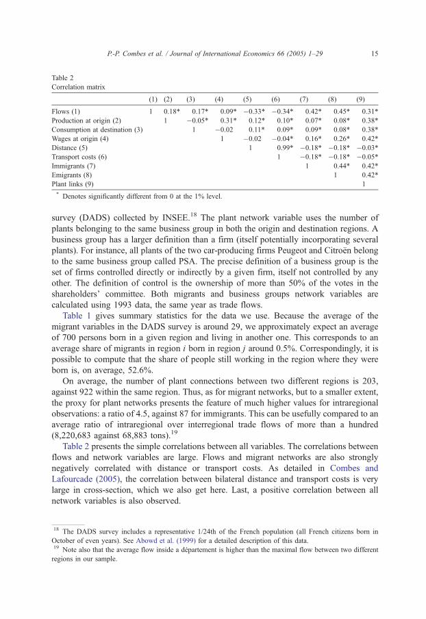
Table 2
Correlation matrix
(1) (2) (3) (4) (5) (6) (7) (8) (9)
Flows (1) 1 0.18* 0.17* 0.09* �0.33* �0.34* 0.42* 0.45* 0.31*
Production at origin (2) 1 �0.05* 0.31* 0.12* 0.10* 0.07* 0.08* 0.38*
Consumption at destination (3) 1 �0.02 0.11* 0.09* 0.09* 0.08* 0.38*
Wages at origin (4) 1 �0.02 �0.04* 0.16* 0.26* 0.42*
Distance (5) 1 0.99* �0.18* �0.18* �0.03*
Transport costs (6) 1 �0.18* �0.18* �0.05*
Immigrants (7) 1 0.44* 0.42*
Emigrants (8) 1 0.42*
Plant links (9) 1
* Denotes significantly different from 0 at the 1% level.
P.-P. Combes et al. / Journal of International Economics 66 (2005) 1–29 15
survey (DADS) collected by INSEE.18 The plant network variable uses the number of
plants belonging to the same business group in both the origin and destination regions. A
business group has a larger definition than a firm (itself potentially incorporating several
plants). For instance, all plants of the two car-producing firms Peugeot and CitroJn belong
to the same business group called PSA. The precise definition of a business group is the
set of firms controlled directly or indirectly by a given firm, itself not controlled by any
other. The definition of control is the ownership of more than 50% of the votes in the
shareholders’ committee. Both migrants and business groups network variables are
calculated using 1993 data, the same year as trade flows.
Table 1 gives summary statistics for the data we use. Because the average of the
migrant variables in the DADS survey is around 29, we approximately expect an average
of 700 persons born in a given region and living in another one. This corresponds to an
average share of migrants in region i born in region j around 0.5%. Correspondingly, it is
possible to compute that the share of people still working in the region where they were
born is, on average, 52.6%.
On average, the number of plant connections between two different regions is 203,
against 922 within the same region. Thus, as for migrant networks, but to a smaller extent,
the proxy for plant networks presents the feature of much higher values for intraregional
observations: a ratio of 4.5, against 87 for immigrants. This can be usefully compared to an
average ratio of intraregional over interregional trade flows of more than a hundred
(8,220,683 against 68,883 tons).19
Table 2 presents the simple correlations between all variables. The correlations between
flows and network variables are large. Flows and migrant networks are also strongly
negatively correlated with distance or transport costs. As detailed in Combes and
Lafourcade (2005), the correlation between bilateral distance and transport costs is very
large in cross-section, which we also get here. Last, a positive correlation between all
network variables is also observed.
18 The DADS survey includes a representative 1/24th of the French population (all French citizens born in
October of even years). See Abowd et al. (1999) for a detailed description of this data.19 Note also that the average flow inside a departement is higher than the maximal flow between two different
regions in our sample.
P.-P. Combes et al. / Journal of International Economics 66 (2005) 1–2916
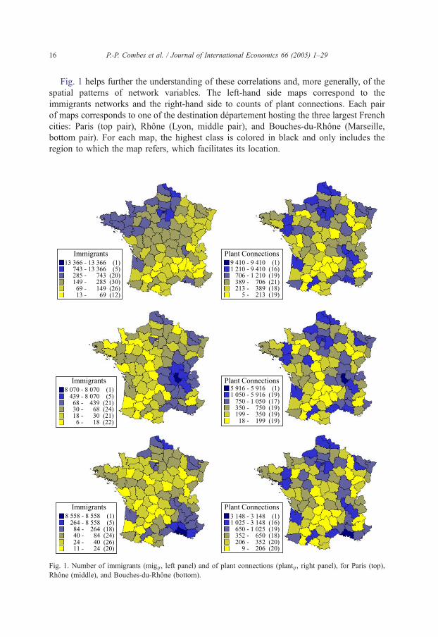
Fig. 1 helps further the understanding of these correlations and, more generally, of the
spatial patterns of network variables. The left-hand side maps correspond to the
immigrants networks and the right-hand side to counts of plant connections. Each pair
of maps corresponds to one of the destination departement hosting the three largest French
cities: Paris (top pair), Rhone (Lyon, middle pair), and Bouches-du-Rhone (Marseille,
bottom pair). For each map, the highest class is colored in black and only includes the
region to which the map refers, which facilitates its location.
Fig. 1. Number of immigrants (migij, left panel) and of plant connections (plantij, right panel), for Paris (top),
Rhone (middle), and Bouches-du-Rhone (bottom).
P.-P. Combes et al. / Journal of International Economics 66 (2005) 1–29 17
The top left map shows that Paris hosts large numbers of migrants originating from
regions either relatively proximate to Paris (North, North-West of France), or more remote
but larger in terms of population (the regions hosting Bordeaux, Lyon, and Marseille
notably). This gravity pattern also clearly emerges for Rhone and Bouches-du-Rhone. The
effect of distance is still strong, but large regions as Paris or Nord appear as major sources
of migrants. Regarding plant links, the impact of distance is less striking. The size of the
origin region, however, still has a clear role, the spatial pattern of plant networks being
quite similar independently of the destination region. Levels change, however. This
conclusion is confirmed by the relatively large correlation between plant links and
production (see Table 2).
4. The trade-creating effect of business and social networks
This section evaluates the statistical significance and economic magnitude of the impact
of business and social networks on trade flows. Results are presented omitting
intraregional trade observations, and therefore abstracting from the analysis of border
effects, covered in the next section.
4.1. Significance and explanatory power of network variables
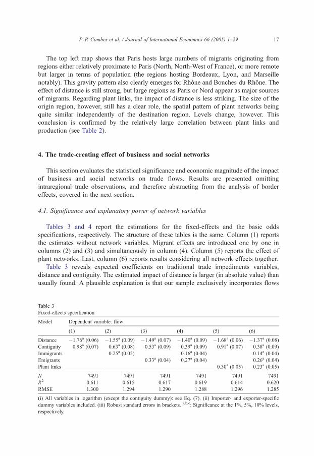
Tables 3 and 4 report the estimations for the fixed-effects and the basic odds
specifications, respectively. The structure of these tables is the same. Column (1) reports
the estimates without network variables. Migrant effects are introduced one by one in
columns (2) and (3) and simultaneously in column (4). Column (5) reports the effect of
plant networks. Last, column (6) reports results considering all network effects together.
Table 3 reveals expected coefficients on traditional trade impediments variables,
distance and contiguity. The estimated impact of distance is larger (in absolute value) than
usually found. A plausible explanation is that our sample exclusively incorporates flows
Table 3
Fixed-effects specification
Model Dependent variable: flow
(1) (2) (3) (4) (5) (6)
Distance �1.76a (0.06) �1.55a (0.09) �1.49a (0.07) �1.40a (0.09) �1.68a (0.06) �1.37a (0.08)
Contiguity 0.98a (0.07) 0.63a (0.08) 0.53a (0.09) 0.39a (0.09) 0.91a (0.07) 0.38a (0.09)
Immigrants 0.25a (0.05) 0.16a (0.04) 0.14a (0.04)
Emigrants 0.33a (0.04) 0.27a (0.04) 0.26a (0.04)
Plant links 0.30a (0.05) 0.23a (0.05)
N 7491 7491 7491 7491 7491 7491
R2 0.611 0.615 0.617 0.619 0.614 0.620
RMSE 1.300 1.294 1.290 1.288 1.296 1.285
(i) All variables in logarithm (except the contiguity dummy): see Eq. (7). (ii) Importer- and exporter-specific
dummy variables included. (iii) Robust standard errors in brackets. a,b,c: Significance at the 1%, 5%, 10% levels,
respectively.

P.-P. Combes et al. / Journal of International Economics 66 (2005) 1–2918
transiting through ground transport means, which has been shown by Disdier and Head
(2004) to yield substantially higher distance coefficients. They show in a meta-analysis of
distance coefficients in gravity equations that papers involving countries belonging to a
single continent have distance coefficient about 0.4 above the average distance effect
estimate. Note also that the distance coefficient gets back to more usual values (around
minus unity) when using the basic odds specification.
Concerning the network effects we are primarily interested in, a first overall conclusion
to be drawn from Tables 3 and 4 is that the impact of business and social networks is
consistent with theoretical predictions and qualitatively similar in all specifications used.
All network variables have a positive and very significant impact on trade flows in the two
specifications.
In terms of explanatory power, we obtain the expected result that the fixed-effects
approach improves the fit compared to the basic odds specification. First, all variables
being computed as differences with respect to the reference region, the variance to be
explained is larger in basic odds than in fixed-effects. The former specification
mechanically reduces the explanatory power of the model, very much as when first-
difference estimations are performed in time-series compared to estimations in levels.
Second, the fixed-effects specification introduces more flexibility in the estimation, as it
does not constrain the origin and destination regions’ influence to be strictly proportional
to production and wages. By contrast, while R2 gains are fairly small when network
variables are introduced in the fixed-effects regressions, they are more substantial in the
basic odds specification. This underlines two points. First, network effects substitute to the
effects of traditional trade impediments more than they explain a new part of the variance
of flows in both specifications, a point we detail in Section 5. Second, the specification of
explanatory variables in strict accordance with theory in the basic odds specification
makes those more orthogonal to each other, which allows a better identification of the
effect of networks.
Table 4
Basic odds specification
Model: Dependent variable: bilateral flow relative to flow from reference region
(1) (2) (3) (4) (5) (6)
Intercept �2.62a (0.15) �2.16a (0.15) �2.04a (0.14) �1.95a (0.15) �2.45a (0.13) �1.98a (0.15)
Distance �1.01a (0.09) �0.79a (0.10) �0.80a (0.10) �0.73a (0.10) �0.95a (0.08) �0.74a (0.09)
Contiguity 2.00a (0.13) 1.56a (0.13) 1.50a (0.11) 1.39a (0.12) 1.84a (0.11) 1.42a (0.12)
Production 0.80a (0.08) 0.60a (0.09) 0.64a (0.08) 0.57a (0.08) 0.43a (0.10) 0.36a (0.10)
Wage �1.76a (0.47) �0.89b (0.37) �3.08a (0.48) �1.96a (0.43) �3.35a (0.58) �2.78a (0.53)
Immigrants 0.30a (0.06) 0.21a (0.07) 0.19a (0.07)
Emigrants 0.32a (0.05) 0.19a (0.05) 0.12b (0.05)
Plant links 0.46a (0.08) 0.31a (0.07)
N 7491 7491 7491 7491 7491 7491
R2 0.366 0.393 0.391 0.400 0.390 0.410
RMSE 1.594 1.560 1.563 1.551 1.564 1.539
(i) All variables in logarithm and computed relatively to the origin corresponding to the highest flow with the
destination (except the contiguity dummy): see Eq. (10). (ii) Robust standard errors in brackets. a,b,c: Significance
at the 1%, 5%, 10% levels, respectively.

P.-P. Combes et al. / Journal of International Economics 66 (2005) 1–29 19
These results all point to the conclusion that business and social networks exert a very
significant positive impact on trade. The similarity of the results is quite striking between
those two fairly different approaches. Network links created by both migrants and business
groups appear to enhance trade. Last, the effects are shown to be at work in both
directions. In region i, the migrants from region j or the links with plants in region j would
favor both imports from and exports to region j.
4.2. The magnitude of the trade-creating effect of networks
Beyond the significance of network effects, even more important is the assessment of
their magnitude and thus of their economic importance. Network effects could well be
significant but simultaneously not account for a large share of trade. Rauch and Trindade
(2002) propose to compute the share of trade created by ethnic Chinese populations.
Following their method, we compute the impact on trade of all network variables, which is
given by:
P1þ zij� �..
; ð14Þ
whereP1þ zij is the average value taken by each network variable (zij=migij, migji, plantij)
and . is the estimate of the corresponding elasticity. Results reported in Table 5 can be read
as follows. Each line corresponds to the specification mentioned. Columns labelled
bSeparateQ (bSimultaneousQ, respectively) report the impact on trade of network variables
when they are introduced in the regression separately (simultaneously, respectively). For
instance, the first figure in line bFixed-effectsQ (column bSeparateQ/bImmigrantsQ) means
that immigrants increase trade by 73.3%, as calculated from the average value of that
variable and the coefficient of a fixed-effects estimation in which this is the only network
variable considered (Table 3, column (2)).
To summarize results, we show that the impact of network variables is:
(i) larger when variables are introduced separately than when introduced simultaneously;
(ii) slightly stronger in the basic odds specification than in the fixed-effects; and
(iii) generally stronger for plant networks than for migrant networks.
Conclusion (i) is quite intuitive because network variables are positively correlated with
each other (see Table 2) and tend to partially exclude each other when introduced
simultaneously. We attribute conclusion (ii) to the fact that the estimated relationship has a
Table 5
Trade creation (in percent (%))
Separate Simultaneous
Immigrants Emigrants Plant links Immigrants Emigrants Plant links
Fixed-effects 73.3 102.3 303.4 36.6 73.8 192.5
Basic odds 91.9 99.2 719.9 52.5 30.0 320.7
Percentage of trade increase computed as given in Eq. (14).

P.-P. Combes et al. / Journal of International Economics 66 (2005) 1–2920
better specification in the basic odds specification, which improves the estimation of
network effects. Conclusion (iii) is a new result: Business networks across locations
associated with economic links between plants have a substantially higher impact on trade
than networks based on migrant connections.
Interestingly, the impact of migrants alone is found to be of the same order of
magnitude as the one estimated by Rauch and Trindade (2002) for ethnic Chinese
populations. The product of Chinese population shares at origin and destination increases
trade in a gravity specification by 60%. The effects of migration, either immigrants or
emigrants, within France, range from 73.3% to 102.3%, a level that is slightly stronger
than the effect of Chinese populations on international trade. The economic impact of
business networks between plants is found to be generally much larger than the impact of
migrants. To the best of our knowledge, this had never been econometrically quantified.
When introduced separately from the migrants, according to the fixed-effects estimation,
links between plants belonging to the same business group would make trade around four
times larger than in the absence of network effects (around eight times larger in the basic
odds specification). These are large numbers.
However, using a single variable to proxy network effects might capture the impact of
other missing network variables. In order to correctly quantify the impact of each
variable, it is thus more consistent to use regressions where all variables are introduced
simultaneously. According to the fixed-effects or the basic odds specifications, when
controlling for plant networks, the impact of each migrant variable is lower than when
introduced alone, but still not negligible: each kind of migrant variable creates between
30.0% and 73.8% of interregional trade, while both kinds together increase trade by
36.6+73.8=110.4% in the fixed-effects specification and 52.5+30.0=82.5% in the basic
odds specification. One can therefore conclude that, in France, the presence of migrants
(from other French regions) roughly doubles interregional trade on average compared to a
hypothetical situation without any mobility of people. The impact of plant networks is
lower than when entered in the regression separately from migrant networks. Still, plant
networks multiply trade by nearly three, in fixed-effects, and more than four, in basic
odds.
Finally, note that it is difficult to state which of the impacts of immigrants or emigrants
is larger. Results on this question vary depending on the considered variable and on the
way the effect is estimated. This is probably due to the collinearity between network
variables. It is therefore difficult to compare the relative magnitude of the preference
effects of networks to their information counterpart using the comparison of immigrants’
and emigrants’ coefficients. However, as proposed above, the use of plant networks here
helps in this identification process. The much larger effect of plant networks points to a
dominance of information effects over preference effects.
5. Can networks explain the border effect puzzle?
We now turn to the estimation of the last two specifications we propose. They both
allow to estimate the effect of administrative borders in France, identified as the
average ratio between intra- and interregional trade flows. This can thus be viewed as

P.-P. Combes et al. / Journal of International Economics 66 (2005) 1–29 21
a way to properly assess the impact of networks on all trade impediments (as opposed
to focusing on barriers taking place between regions only—captured by distance and
contiguity). The main difference between the basic and the complete odds
specifications relies on the fact that the reference flow is the internal one in the
complete version. The friction approach is more sensibly different because both the
dependent and the explanatory variables are computed as the product of the variables
that enter the odds specifications. Note also that we now use the real measure of
transport costs (and its square) instead of its potentially noisy proxy constituted by
distance.
There are advantages and drawbacks to the new approaches presented in this section.
On the one hand, more data is needed. On the other hand, one might expect more robust
results: endogeneity concerns for regional sizes and wages for instance disappear in the
friction specification and transport cost data should do a better job than distance at
isolating the transport cost effects from the impact of networks. Second, new results are
provided in terms of the impact of administrative borders on trade and of networks on
this border effect. Indeed, as recalled in the Introduction, even elaborated methodologies
have not succeeded in solving entirely the border effect puzzle. We investigate here
whether network effects could be part of the explanation why borders seem to matter so
much for trade patterns. The theoretical literature is actually fairly agnostic on the
question of whether networks should impact trade (log) linearly with distance or not. If
networks do not spill over borders and are bounded inside the regions where they are
located, they could be responsible for the measured border effect. Border effects would
consequently be a sort of statistical illusion, reflecting the bounded nature of networks
following administrative borders, rather than a brealQ cost incurred at the physical border.
Table 6
Complete odds specification
Model Dependent variable: bilateral flow relative to internal flow
(1) (2) (3) (4) (5) (6)
Intercept �1.84a (0.16) �1.30a (0.16) �1.15a (0.18) �1.02a (0.18) �1.50a (0.15) �1.08a (0.17)
Production 0.55a (0.06) 0.41a (0.06) 0.41a (0.06) 0.37a (0.06) 0.30a (0.07) 0.24a (0.07)
Wage �1.99a (0.43) �1.01a (0.34) �2.60a (0.44) �1.89a (0.46) �3.35a (0.46) �3.09a (0.48)
Transport
costs
�2.31a (0.11) �1.92a (0.16) �1.83a (0.14) �1.73a (0.15) �2.03a (0.12) �1.74a (0.15)
Transport
costs sq.
2.5e-8a (0.8e-8) 1.3e-8 (0.9e-8) 1.1e-8 (0.8e-8) 0.8e-8 (0.8e-8) 1.2e-8 (0.8e-8) 0.5e-8 (0.9e-8)
Contiguity 0.88a (0.08) 0.67a (0.08) 0.61a (0.09) 0.56a (0.08) 0.87a (0.07) 0.69a (0.08)
Immigrants 0.23a (0.04) 0.13a (0.05) 0.07 (0.05)
Emigrants 0.29a (0.05) 0.22a (0.05) 0.14b (0.05)
Plant links 0.48a (0.05) 0.39a (0.05)
N 7491 7491 7491 7491 7491 7491
R2 0.422 0.436 0.440 0.443 0.454 0.460
RMSE 1.518 1.500 1.495 1.490 1.475 1.467
(i) All variables in logarithm and computed relatively to the value for the destination region itself (except the
contiguity dummy): see Eq. (11). (ii) Robust standard errors in brackets. a,b,c: Significance at the 1%, 5%, 10%
levels, respectively.
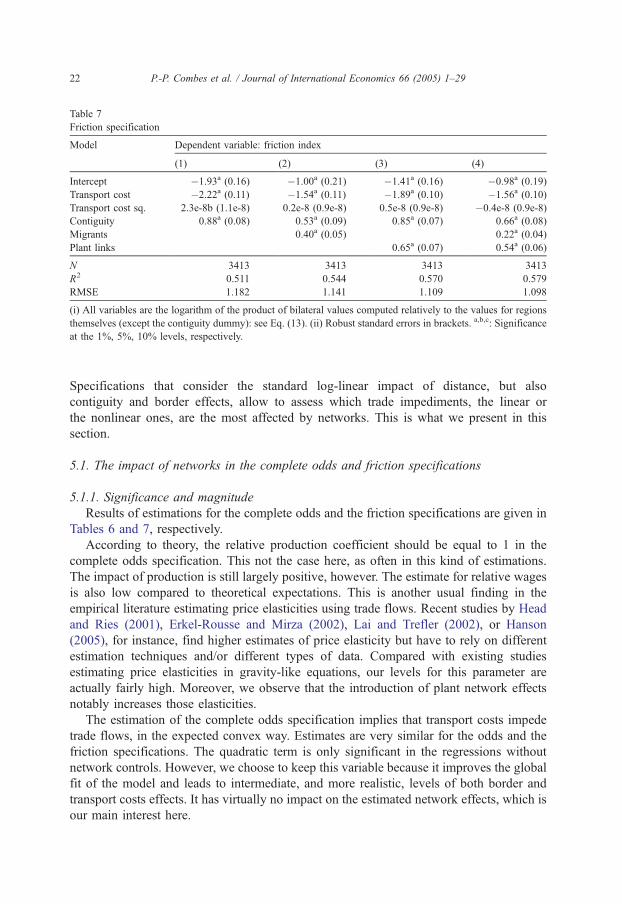
Table 7
Friction specification
Model Dependent variable: friction index
(1) (2) (3) (4)
Intercept �1.93a (0.16) �1.00a (0.21) �1.41a (0.16) �0.98a (0.19)
Transport cost �2.22a (0.11) �1.54a (0.11) �1.89a (0.10) �1.56a (0.10)
Transport cost sq. 2.3e-8b (1.1e-8) 0.2e-8 (0.9e-8) 0.5e-8 (0.9e-8) �0.4e-8 (0.9e-8)
Contiguity 0.88a (0.08) 0.53a (0.09) 0.85a (0.07) 0.66a (0.08)
Migrants 0.40a (0.05) 0.22a (0.04)
Plant links 0.65a (0.07) 0.54a (0.06)
N 3413 3413 3413 3413
R2 0.511 0.544 0.570 0.579
RMSE 1.182 1.141 1.109 1.098
(i) All variables are the logarithm of the product of bilateral values computed relatively to the values for regions
themselves (except the contiguity dummy): see Eq. (13). (ii) Robust standard errors in brackets. a,b,c: Significance
at the 1%, 5%, 10% levels, respectively.
P.-P. Combes et al. / Journal of International Economics 66 (2005) 1–2922
Specifications that consider the standard log-linear impact of distance, but also
contiguity and border effects, allow to assess which trade impediments, the linear or
the nonlinear ones, are the most affected by networks. This is what we present in this
section.
5.1. The impact of networks in the complete odds and friction specifications
5.1.1. Significance and magnitude
Results of estimations for the complete odds and the friction specifications are given in
Tables 6 and 7, respectively.
According to theory, the relative production coefficient should be equal to 1 in the
complete odds specification. This not the case here, as often in this kind of estimations.
The impact of production is still largely positive, however. The estimate for relative wages
is also low compared to theoretical expectations. This is another usual finding in the
empirical literature estimating price elasticities using trade flows. Recent studies by Head
and Ries (2001), Erkel-Rousse and Mirza (2002), Lai and Trefler (2002), or Hanson
(2005), for instance, find higher estimates of price elasticity but have to rely on different
estimation techniques and/or different types of data. Compared with existing studies
estimating price elasticities in gravity-like equations, our levels for this parameter are
actually fairly high. Moreover, we observe that the introduction of plant network effects
notably increases those elasticities.
The estimation of the complete odds specification implies that transport costs impede
trade flows, in the expected convex way. Estimates are very similar for the odds and the
friction specifications. The quadratic term is only significant in the regressions without
network controls. However, we choose to keep this variable because it improves the global
fit of the model and leads to intermediate, and more realistic, levels of both border and
transport costs effects. It has virtually no impact on the estimated network effects, which is
our main interest here.

P.-P. Combes et al. / Journal of International Economics 66 (2005) 1–29 23
Both the magnitude and the significance of network effects are similar to those
obtained in the specifications presented in Section 4. Considering internal flows and
border, effects do not alter the previous conclusions regarding the trade-creating impact of
networks. In terms of trade creation, the six figures of Table 5 for the complete odds
specification would be 65.4%, 86.7%, 821.5%, 15.6%, 34.5%, and 494.7% which
corresponds to the same magnitude as what is obtained with the basic odds
specification. Migrant network effects are slightly smaller, however, and the impact
of the plant networks is larger in the regression where all effects are introduced
simultaneously. We thus confirm our previous finding that the magnitude of trade
creation is much larger for plant networks than for migrant ones, which tends to support
the information channel.
In order to improve our understanding of the magnitude of the impact of networks,
Table 8 computes, for the average region, the (inverse) of the relevant term in Eq. (11):
P1þ zij
1þ zii
� � !..
; ð15Þ
whereP1þzij1þzii
� �is the average across regions of the impact of each network variable
(zij=migij, migji, plantij) and . is the corresponding elasticity. The impact of both migrant
(or plant) networks, or of all effects together, is also computed by summing these network
effects, which are evaluated, however, with the estimates of the regressions that consider
the effects of network variables simultaneously. We proceed similarly with the friction
specification (Eq. (13)).
The first figure in line bOddsQ of Table 8 means that differences across regions in
the number of immigrants relative to the number of people working in the region
where they were born make, for the average region and when entering the regression
separately, interregional trade flows 3.5 times lower than internal ones. As can be seen
in column bBothQ, migrant network variables acting simultaneously but not controlling
for plant networks would make inter-regional trade flows 6.5 lower than internal ones.
The average difference between inter- and intraregional plant networks lowers
interregional trade by a factor of 2.2 when migrant networks are not controlled for.
The hierarchy between the effects of migrant and plant networks therefore depends on
the benchmark considered. When comparing interregional flows, plant networks are
clearly dominant. On the contrary, when explaining the average surplus of trade taking
Table 8
Network effects
Separate Simultaneous
Migrants Plant links Migrants Plant links All
Immigrant Emigrant Both Immigrant Emigrant Both
Odds 3.5 4.8 6.5 2.2 1.4 2.1 3.0 1.9 5.7
Friction – – 8.3 2.9 – – 3.3 2.4 7.9

P.-P. Combes et al. / Journal of International Economics 66 (2005) 1–2924
place within administrative borders, the effects are reversed, suggesting that the spatial
distribution of migrants is more governed by administrative borders than the
distribution of plants.
When all network variables are considered simultaneously (right-hand side of Table 8,
columns bSimultaneousQ), the impact of migrant networks appears to be more than twice
smaller, while the impact of plant networks decreases by less than 20%. Migrant and plant
network effects are of comparable magnitude. Finally, all network effects together make
interregional flows 5.7 times lower than intraregional ones now. The impact of networks in
shaping trade flows is even larger according to the friction specification, which is our
favourite estimation because it corrects for the potential endogeneity of production and
wage variables. Business and social networks would make interregional flows nearly eight
times lower than intraregional ones in this case.
5.1.2. Endogeneity
There are two potential sources of endogeneity for the network variables.20 One is
linked to potentially omitted variables. An unobserved positive productivity shock in a
region for instance may simultaneously raise trade flows and attract new plants or
migrants, which induces a correlation between the error term and the network
variables. The second source of endogeneity is linked to reverse causality. Large
merchandize flows may mean that potential migrants will find the commodities they
like in the destination region, which triggers migration. Similarly, firms might use the
trade flow signal to take their location decision, anticipating, for instance, that they
will find partners in the destination region, that production conditions are good, etc.
In both cases, causality would go from trade flows to networks, biasing OLS
estimates.
The way we address the potential endogeneity of network variables is twofold. First,
the trade variable is a yearly flow whereas network variables correspond to total stocks
of migrants and plants present in the region. This should reduce both the simultaneity
and the reverse causality issues. Second, we perform some regressions where the 1993
migrant network variables are instrumented with their 1978 values. Since those
correspond to stocks again, furthermore, computed 15 years earlier than the date at
which commodity flows are observed, we think they provide good instruments for
migrant networks. Due to lack of space, instrumented regressions are presented in details
in the working paper version (Combes et al., 2004), and we only comment on the main
results here. The explanatory power of instruments is high. Depending on the regression,
migrant network variables are or not endogenous which shows that questioning possible
endogeneity is indeed important. However, here, endogeneity appears to leave the
estimations unaffected: if anything, endogeneity appears to introduce a downward bias
only. All coefficients for migrant network variables are larger, even if slightly so in most
cases, when instrumented. We are thus confident that our results are not caused by
endogeneity issues.
20 Endogeneity of other variables in bilateral trade estimations has been rarely investigated, Harrigan (1996)
being one exception. Recall that our friction specification is immune to such biases.
P.-P. Combes et al. / Journal of International Economics 66 (2005) 1–29 25
5.2. The decline in the estimates of trade impediments
5.2.1. Border effects without network controls
The line binterceptQ in Table 6 gives the coefficient needed to calculate the effect of
administrative borders in France: �1.84 in column (1) means that interregional flows
between two non contiguous regions are exp(1.84)=6.3 times lower than intraregional
ones ceteris paribus, when network effects are not controlled for in the complete odds
specification. Column (1) in Table 7 reports the estimates for the friction specification
without networks effects and leads to a very similar value. The border effect is evaluated
at exp(1.93)=6.9. Interestingly, both values are only slightly larger than what Wolf
(2000) finds for trade inside the United States in 1993, which is also the year we
consider.
The contiguity variable allows to distinguish between two different kinds of border
effects. The estimate reported in line bcontiguityQ in Table 6 means that, according to the
estimation of the complete odds specification, interregional trade flows between two
noncontiguous regions are exp(0.88)=2.4 times lower than flows between two contiguous
ones. Therefore, trade between two contiguous regions are exp(1.84�0.88)=2.6 times
lower than internal trade flows, which we call the blocal border effectQ. In other words, the
border effect can be decomposed as: 6.3=2.4�2.6.21 Both drops in trade flows are of
similar magnitude. Note also that the estimate of the contiguity effect is exactly the same
in the friction specification.22
5.2.2. The impact of networks on the distance, border, and contiguity effects
Table 9 computes the changes in trade impediments when network variables are
introduced. The first three lines correspond to estimates from the complete odds
specification. For instance, the first figure indicates that when only immigrants networks
are controlled for in the odds specification, the total border effect varies by
[exp(1.30�1.84)�1]=�42.1%, 1.84 and 1.30 being the estimates of the border effects
taken from Table 6 columns (1) and (2), respectively. The other figures of the line are
similarly computed with the other estimations. A similar procedure is then applied for the
effect of contiguity.23 The last line gives the variation for the average region of the
transport cost effect given by the (inverse of the) exponential of:
rdln
"P1þ tij
1þ tii
� �#þ rhPt2ij � t2ii
� �� �: ð16Þ
21 Note that 2.4�2.6 is not strictly equal to 6.3 because we present rounded figures.22 Changing the definitions of the internal transport cost, or including or not the contiguity dummy, modifies the
magnitude of the border effect. This is mechanical because it directly corresponds to a translation in the intercept
of the regression as is now well-established (see Wei, 1996, and Helliwell and Verdier, 2001, for instance). Our
primary interest here is the way trade impediments are affected by networks. And indeed, we find this impact to
be very similar across variants regarding distance, contiguity, and border variables, the reason why we concentrate
our presentation on one variant only.23 The variation of the contiguity effect is part of the variation of the border effect.

Table 9
Network impact on distance, border, and contiguity effects
Separate Simultaneous
Migrants Plant links All
Immigrant Emigrant Both
Odds Border (%) �42.1 �49.9 �56.3 �29.0 �53.3
Contiguity(%) �18.7 �23.0 �26.9 �0.8 �17.3
Transport (%) �47.2 �55.1 �61.8 �31.5 �58.0
Friction Border (%) – – �60.4 �40.3 �61.4
Contiguity(%) – – �29.2 �2.5 �19.4
Transport (%) – – �70.4 �41.5 �67.8
P.-P. Combes et al. / Journal of International Economics 66 (2005) 1–2926
whereP1þtij1þtii
� �is the average across regions of the linear impact of the transport cost, and,
similarly, of the quadratic impact.
The last column in Table 9 shows that when introduced simultaneously, business and
social networks have a strong impact on the border effect that decreases by 53.3% and
61.4% according to the complete odds and the friction specifications, respectively. Migrant
networks make border effects decline slightly more than plant networks. Thus, the
bnetwork-partQ of the usually estimated border effects would be more caused by missing
migrant network variables than by plant network ones.
Second, the lines labelled bContiguityQ show that both components of the border effect
(the local border effect and contiguity) are affected by networks. However, the local
border effect variation is three times stronger than the contiguity one when all network
variables are introduced simultaneously either in the complete odds or in the friction
specifications. This can be interpreted as evidence that the effects of networks are
stronger at very short distances than at intermediate ones. This is all the more true for
plant networks for which the impact on the contiguity effect is virtually nil. The impacts
of migrant networks are more balanced between the local border and the contiguity
effects.
When network effects are not considered, the impact of transport costs for the
average region, given by the mean of the transport cost effect given in Eq. (16), is equal
to 88. This means that the difference between interregional and intraregional transport
costs causes, for the average region, inter-regional trade flows to be 88 times lower than
internal flows. Thus, transport costs largely impede trade, even when border effects are
taken into account (with an impact much stronger than the one of borders actually).
Noticeably, as reported in line bOddsQ/bTransportQ of Table 9, the decline of the
transport cost impact is equal to 58.0% when all network effects are considered in the
complete odds specification estimation. The magnitude of this decline is comparable to
the border effect reduction. Emigrants also have a slightly stronger impact than
immigrants. Last, the reduction implied by migrant networks only is twice as large as
the one by plant networks (61.8% versus 31.5%). Again, this would mean that the
spatial scope of migrant networks is wider, while plant networks would have more of a
nonlinear impact mainly acting on short distances. Similar conclusions can be drawn
from the estimations of the friction specification, the implied variations being slightly
larger.

P.-P. Combes et al. / Journal of International Economics 66 (2005) 1–29 27
6. Conclusion
We quantify in this paper the trade-creating effects of business and social networks
emphasized recently by trade economists as an important theoretical and empirical
determinant of international transactions. The results we obtain for the impact of
migrations confirm the existing evidence in the literature. The average observed level of
migrant stocks doubles trade flows compared to a situation without migration. While these
migrant effects can be explained by both preference and information effects, we also
provide new results regarding pure information business effects captured by the intensity
of the links between plants belonging to the same business group. These links multiply
trade flows by as much as four. These estimates are obtained under several and quite
different methodologies, some of them instrumenting the possibly endogenous migrant
network variables. The larger impact of plant networks, which cannot be attributed to
preference effects, suggests that the information channel could be the main vector of the
impact of networks.
We also show that network effects, when omitted, are captured to a wide extent by the
set of variables that embody the impact of spatial proximity on trade flows (transport
costs, borders, and contiguity). Consequently, our results point to a potential over-
estimation in the literature of the effects of these variables. For instance, the impact of
transport costs is reduced by as much as 68% when network controls are introduced. The
unexplained remaining border effect is estimated to multiply internal flows by bonlyQ2.7, compared to interregional flows between two non-contiguous regions. This ratio is
equal to 6.9 when network variables are omitted. Although those multiplicative factors
could still seem to be large numbers for a country as integrated as France, they are
comparable to what Wolf (2000) finds for the effect of states’ borders inside the United
States.
Improvements in the quantification of the role of business and social networks on trade
can take several forms. First, progress can be made in terms of the variety of network
proxies and instruments used. Next, attempts to improve the separate identification of
information and preference effects should be continued. Last, and more generally, the
theoretical underpinnings of the network block of our trade model could also be improved
in order to provide more structure to this part of the estimation.
Acknowledgement
This paper is produced as part of a CEPR Research Network on The Economic
Geography of Europe: Measurement, Testing and Policy Simulations, funded by the
European Commission under the Research Training Network Programme (Contract No:
HPRN-CT-2000-00069). We thank Jean-Eric Thomas for having kindly made the trade
flow data available to us. We are also grateful to Johannes Brfcker, Harry Flam, Laurent
Gobillon, Keith Head, Christiane Krieger-Boden, and to seminar participants (ERWIT
2002, HWWA Workshop on border regions 2002, and the Econometric Society North
American 2004 Winter Meetings) for fruitful comments and discussions. Comments by a
coeditor and two anonymous referees were crucial in the improvement of the paper. We

P.-P. Combes et al. / Journal of International Economics 66 (2005) 1–2928
gratefully acknowledge the hospitality of the French Ministry of Transport Economics
Department (SES-DAEI) and of Boston University, as well as the financial support from
SES-DAEI and from NATO (Combes’ advanced fellowship grant).
References
Abowd, J., Kramarz, F., Margolis, D., 1999. High wage workers and high wage firms. Econometrica 67,
251–333.
ACFCI, 2002, Rapport annuel d’activites des CCI. http://www.acfci.cci.fr/presentationACFCI/index.htm#rac02.
Anderson, J., van Wincoop, E., 2003. Gravity with gravitas: a solution to the border puzzle. American Economic
Review 93, 170–192.
Anderson, S., De Palma, A., Thisse, J.-F., 1992. Discrete Choice Theory of Product Differentiation. MIT Press,
Cambridge.
Belderbos, R., Sleuwaegen, L., 1998. Tariff jumping DFI and export substitution: Japanese electronics firms in
Europe. International Journal of Industrial Organization 16 (5), 601–638.
Chen, N., 2004. Intra-national versus international trade in the European Union: why do national borders matter?
Journal of International Economics 63 (1), 93–118.
Combes, P.-P., Lafourcade, M., 2005. Transport costs: measures, determinants and regional policy implications
for France, forthcoming in the Journal of Economic Geography.
Combes, P.-P., Lafourcade, M., Mayer, T., 2004. The trade creating effects of business and social networks:
evidence from France. CERAS Working Paper 04-04.
Disdier, A.-C., Head, K., 2004. Exaggerated reports of the death of distance: lessons from a meta-analysis. mimeo
U. of Paris 1 (http://team.univ-paris1.fr/teamperso/disdier/meta.pdf ).
Dixit, A., Stiglitz, J., 1977. Monopolistic competition and optimum product diversity. American Economic
Review 67 (3), 297–308.
Eaton, J., Kortum, S., 2002. Technology, geography and trade. Econometrica 70 (5), 1741–1780.
Erkel-Rousse, H., Mirza, D., 2002. Import price-elasticities: reconsidering the evidence. Canadian Journal of
Economics 35 (2), 282–306.
Ethier, W., 1982. National and international returns to scale in the modern theory of international trade. American
Economic Review 72, 389–405.
Feenstra, R., 2003. Advanced International Trade: Theory and Evidence. Princeton University Press, Princeton.
Girma, S., Yu, Z., 2002. The link between immigration and trade: evidence from the United Kingdom.
Weltwirtschaftliches Archiv 138 (1), 115–130.
Gould, D., 1994. Immigrant links to home country: empirical implications for US bilateral trade flows. Review of
Economics and Statistics 76, 302–316.
Hanson, G., 2005. Market potential, increasing returns, and geographic concentration, forthcoming in the Journal
of International Economics.
Harrigan, J., 1996. Openness to trade in manufactures in the OECD. Journal of International Economics 40 (1–2),
23–39.
Head, K., Mayer, T., 2000. Non-Europe: the magnitude and causes of market fragmentation in Europe.
Weltwirtschaftliches Archiv 136 (2), 285–314.
Head, K., Ries, J., 2001. Increasing returns versus national product differentiation as an explanation for the
pattern of US–Canada trade. American Economic Review 91 (4), 858–876.
Head, K., Ries, J., Spencer, B., 2004. Vertical networks and U.S. auto parts exports: is Japan different? Journal of
Economics and Management Strategy 13 (1), 37–67.
Helliwell, J., 1996. Do national borders matter for Quebec’s trade? Canadian Journal of Economics 29 (3),
507–522.
Helliwell, J., 1997. National borders, trade and migration. Pacific Economic Review 3 (3), 165–185.
Helliwell, J., Verdier, G., 2001. Measuring internal trade distances: a new method applied to estimate provincial
border effects in Canada. Canadian Journal of Economics 34 (4), 1024–1041.
Hillberry, R., Hummels, D., 2003. Intra-national home bias: some explanations. Review of Economics and
Statistics 85 (4), 1089–1092.

P.-P. Combes et al. / Journal of International Economics 66 (2005) 1–29 29
Hummels, D., 1999. Towards a geography of trade costs, Krannert School of Management mimeo, http://
www.mgmt.purdue.edu/faculty/hummelsd/research/toward/Toward3.pdf.
INSEE, 2001. Le zonage en aires urbaines en 1999: 4 millions d’habitants en plus dans les aires urbaines. INSEE
Premiere 765 (4 p.).
Krugman, P., 1980. Scale economies, product differentiation, and the pattern of trade. American Economic
Review 70, 950–959.
Lai, N., Trefler, D., 2002. The gains from trade with monopolistic competition: specification, estimation, and mis-
specification, NBER Working 9169.
Lawrence, R., 1993. Japan’s different trade regime: an analysis with particular reference to keiretsu. Journal of
Economic Perspectives 7 (3), 3–19.
Limao, N., Venables, A., 2001. Infrastructure, geographical disadvantage, transport costs and trade. World Bank
Economic Review 15 (3), 451–479.
McCallum, J., 1995. National borders matter: Canada–US regional trade patterns. American Economic Review
85, 615–623.
Ministry of the Interior (DGCL), 2003, Budgets primitifs des departements 2003. http://www.dgcl.interieur.
gouv.fr/Publications/budgets_primitifs_departements_2003/accueil_budget_departements_2003.htm.
Nitsch, V., 2000. National borders and international trade: evidence from the European Union. Canadian Journal
of Economics 22 (4), 1091–1105.
Obstfeld, M., Rogoff, K., 2000. The six major puzzles in international macroeconomics: is there a common
cause? In: Bernanke, B., Rogoff, K. (Eds.), NBER Macroeconomics Annual 2000.
Parsley, D., Wei, S.-J., 2001. Explaining the border effect: the role of exchange rate variability, shipping costs and
geography. Journal of International Economics 55 (1), 87–105.
Rauch, J., 2001. Business and social networks in international trade. Journal of Economic Literature 39,
1177–1203.
Rauch, J., Trindade, V., 2002. Ethnic Chinese networks in international trade. Review of Economics and Statistics
84 (1), 116–130.
Redding, S., Venables, A., 2004. Economic geography and international inequality. Journal of International
Economics 62 (1), 53–82.
Rose, A., 2000. One money, one market: the effect of common currencies on trade. Economic Policy 15 (30),
7–46.
Taglioni, D., 2002. Exchange rate volatility as a barrier to trade: new methodologies and recent evidence.
Economie Internationale 89/90, 227–259.
Wagner, D., Head, K., Ries, J., 2002. Immigration and the trade of provinces. Scottish Journal of Political
Economy 49 (5), 507–525.
Wei, S.-J., 1996. Intra-national versus international trade: how stubborn are nations in global integration? NBER
Working Paper, 5531.
Wolf, H., 2000. Intranational home bias in trade. Review of Economics and Statistics 82 (4), 555–563.