the tradeo s in leaning against the wind - imf · the tradeo s in leaning against the wind {...
TRANSCRIPT
The Tradeoffs in Leaning Against the Wind∗
– Conference Draft –
Francois Gourio† Anil K Kashyap‡ Jae Sim§
October 28, 2016
Abstract
Credit booms sometimes lead to financial crises which are accompanied with severe and
persistent economic slumps. Does this imply that monetary policy should “lean against the
wind” and counteract excess credit growth, even at the cost of higher output and inflation
volatility? We study this issue quantitatively in a standard small New Keynesian dynamic
stochastic general equilibrium model which includes a risk of financial crisis that depends on
“excess credit”. We compare monetary policy rules that respond to the output gap to rules that
respond to excess credit. We find that leaning against the wind may be attractive, depending on
several factors, including (1) the severity of financial crises; (2) the sensitivity of crisis probability
to excess credit; (3) the volatility of excess credit.
1 Introduction
The question of whether financial stability concerns should play a role in the setting of monetary
policy has generated a vigorous debate. In this paper we investigate the wisdom of what has come
to be known as “leaning against the wind” (LAW), that is having monetary policy react to perceived
financial imbalances such as excess credit growth.
There are broadly two types of arguments that have been put forward to reason against LAW.
One critique observes that financial imbalances are difficult to detect and that they are best ad-
dressed with other tools such as prudential (or perhaps even time-varying macro-prudential) policy.
∗The views expressed in this paper do not necessarily reflect the views of the Federal Reserve System, the FederalReserve Board, the Federal Reserve Bank of Chicago, or the Bank of England. We are responsible for all errors.†The Federal Reserve Bank of Chicago. Email: [email protected]‡The University of Chicago Booth School of Business and the Bank of England. Email:
[email protected]§The Board of Governors of the Federal Reserve System. Email: [email protected]
1

Monetary policy is presumed to have small and uncertain effects on financial imbalances and when
weighed against the usual costs of slowing the economy the trade-off is unfavorable (Bernanke and
Gertler (1999)).1
Svensson (2016) goes further and argues that it is appropriate to account for the fact that the
costs of a crisis can differ depending on the initial conditions that prevail prior to the crisis onset.
If the economy is starting from a fragile position, the crisis can be more costly. Because LAW
weakens the economy, this is an additional argument against it. He argues that monetary policy
should remain focused on inflation and output stability.
There are also at least two alternative rationales that have been offered in favor of LAW.2 As
Reinhart and Rogoff (2009) and Cerra and Saxena (2008) emphasized even before the most recent
crisis, recovery from crises are typically slow so that the hangover from a crisis is different than
from a regular recession. It is routine to see charts in the popular press showing that there seems
to be a large downward shift in the level of GDP. Preventing a crisis may, therefore, bring different
benefits than those associated with smoothing out inefficient business cycle fluctuations (See Barro
(2009)). As will see this consideration features prominently in our analysis.
The second concern, as recently expressed by Dudley (2015), is that the appeal to use macro-
prudential tools as a first line of defense against financial imbalances is much easier said than done.
Many countries such as the United States have a limited set of macro-prudential tools, and these
tools are difficult to adjust; and monetary policy has broad effects (it “gets in all the cracks” as
Stein (2013) famously noted) while macro-prudential tools are perhaps too narrow (e.g. they lead
to a migration of activities from the regulated banking system to the unregulated shadow banking
system). This consideration motivates our focus of monetary policy.
Our main contribution is to propose a stylized Dynamic Stochastic General Equilibrium (DSGE)
to assess the efficacy of LAW. We depart from the usual model in two ways. First, we follow Gourio
(2012) and introduce a standard capital structure choice based on the trade-off theory. Capital is
accumulated by firms that face costs of issuing equity, while debt is subsidized by the tax code
1A distinct argument states that it is preferable to “mop up after the crash”, but this argument seems lesscompelling now in light of the difficulties in stabilizing the economy in the aftermath of the most recent financialcrises - for instance, the zero lower bound and reduced potency of monetary policy when agents want to deleverage.
2Peek, Rosengren, and Tootell (2015) also add a political economy consideration that is outside the scope of ouranalysis. As they note, crises often involve bank rescues that generate political backlash which can make it difficultfor central banks to conduct monetary policy going forward.
2

and in the event of default there are deadweight costs to bankruptcy. The combination of the tax
subsidy and the equity issuance costs leads the firms to over-rely on debt financing. In what follows
we refer to the over-reliance as ”excess credit” or ”inefficient credit”.
We introduce a “financial shock” in this economy by assuming that the tax benefit varies over
time. As we explain below, this is a shorthand for various forms of inefficient credit use. We view
the tradeoff theory as providing a compact way to introduce variation in the use of debt financing
(that could in fact arise for many reasons). What is more important is the potential problems that
can arise from the excess credit due to our second modification.
The second modification is to introduce the possibility of a large financial crisis that can hit the
economy. This is similar to the rare disasters that have received much attention recently in the asset
pricing literature.3 We assume that the financial crisis leads to a significant, permanent reduction
in total factor productivity and a one-off shock to the capital stock. We view this modeling as
a convenient device to capture that financial crises lead to large and highly persistent declines in
output and consumption. Given that there is not much of a consensus as why crises are so costly,
this simplification seems like a reasonable way to model then without taking a stand on a particular
reason why losses seem to be so persistent.
We study two types of collapses. The first kind of financial crisis, as in Gourio (2012) and
Gourio (2013), occurs exogenously. The second supposes that the probability of the crisis depends
on the amount of inefficient credit. By comparing the two alternatives we can isolate the policy
consequences of living with possibility of large crises from the possibility that leaning against the
wind might be able to change the likelihood of a crisis.
The model allows for the usual productivity and demand shocks in addition to the financial
shocks. The centerpiece of the analysis is a comparison of different monetary policy rules that
vary with respect to the signals on which the central bank’s policy rate is set. In our baseline, we
compare policies that rely on perfectly measuring variables and then in some extensions analyze
what happens when the central bank must rely on imperfectly measured proxies. In this respect we
follow in the long line of papers starting with Bernanke and Gertler (1999) and Gilchrist and Leahy
(2002) that ask whether monetary policy should take account of asset price movements. A common
conclusion in that literature is that after accounting for movements in inflation, and possibly output,
3See Barro (2006), Gabaix (2012), Tsai and Wachter (2015) and Gourio (2012).
3

there is no need to respond to asset prices. We explore whether the same conclusion holds in our
environment.
Our main finding is that gains from responding to credit movements depend importantly on the
relative importance of the shocks hitting the economy and the nature of the financial crisis risk. In
some versions of the model, for instance when only productivity and demand shocks are present,
the possibility of a crisis (endogenous or not) makes little difference for policy. In this environment,
stabilizing inflation is optimal. Loosely speaking, once the central bank eliminates demand shocks
and accommodates productivity shocks, it can stabilize inflation and simultaneously control crisis
risk to the extent possible. In this setup, even if financial crises are endogenous it will make little
difference in the policy choices because when the central bank controls demand it will also control
credit and limits crisis risk. This result is consistent with the previous literature, in particular
Bernanke and Gertler (1999).
On the other hand, when there are also shocks to credit, then failure to respond to credit build
ups leads to larger crisis risk than when policy responds to credit developments. Because crises are
very costly, the optimal policy tradeoffs leaning against the wind to reduce crisis risk against the
costs of enduring larger fluctuations in output and inflation. We emphasize that this result does
not require assuming that monetary policy has a very strong effect on the risk of financial crisis.
Moreover this result is symmetric: the central bank responds to excessive credit tightening by
loosening as well as to excessively loose credit by tightening policy. By smoothing the probability
of financial crisis, the central bank generates welfare gains. In part these welfare gains come about
because it reduces the average probability of crisis. This reduction is small but the welfare benefits
are significant given the large cost of financial crises. We detail these mechanisms in more detail
below and provide a preliminary quantitative assessment.
The remainder of the paper proceeds as follows. In the next section, we provide a very brief
literature review. In section 3, we introduce the model. Most elements are very standard and are
common to many New Keynesian models. In presenting the model, therefore, we concentrate on
the two novel aspects mentioned above. Section 4 discusses the parameters used and examines basic
properties of the model economy. Finally, in section 5, we compare the performance of a number
of policy rules for different versions of the model, and illustrate how several key parameters affect
our results. Section 6 concludes.
4
2 Literature Review
Smets (2014) provides an excellent survey of most of the research on leaning against the wind
through 2014, so we summarize his main conclusions and then focus on the most notable papers
since then in our review. We refer interested readers to his paper and here just briefly summarize
the main points that he emphasizes. He starts with a common point that is agreed on most
participants in this debate (including us), that the case for using monetary policy to promote
financial stability depends in part on the availability and effectiveness of other tools. He reviews
a number of analyses, most notably Lim, Costa, Columba, Kongsamut, Otani, Saiyid, Wezel,
and Wu (2011), that study the experience using macroprudential tools and reaches two important
conclusions: that “the empirical literature tentatively supports the effectiveness of macroprudential
tools in dampening procyclicality” and “to what extent such measures are effective enough to
significantly reduce systemic risk is, however, as yet unclear.”
Given the ambiguity over whether financial stability can be delivered without appealing to
monetary policy, he then turns to the question of what the evidence says regarding the effectiveness
of monetary policy in limiting the build up of financial vulnerabilities. Here again he finds mixed
evidence. On the one hand, there are a variety of studies that link higher risk-taking by banks with
looser monetary policy. He stresses that the risk-taking can occur on both the asset-side of the
banks’ balance sheet as they reach for yield and through funding choices that entail extra reliance on
short-term financing. He argues that although there is ample evidence of risk-taking, the question
of whether actively using monetary policy to head it off creates too much collateral damage remains
open. He cites several articles that suggest, for instance, that using monetary policy to forestall
property price booms would have created a recession. Overall we read his paper as suggesting that
there may be scope for leaning against the wind, but doing so would entail non-trivial risks.4
Perhaps the most prominent paper written after the Smets survey is Svensson (2016). He
provides a simple and transparent framework for evaluating LAW policies. He starts with empirical
estimates of the effects of higher interest rates on the likelihood of a crisis (obtained by combining
estimates of the effect of interest rates on credit, and of credit growth on the likelihood of crisis
4Smets also stresses that if the central bank is given responsibility for financial stability and fails to achieve it, thatthe bank’s monetary independence could be compromised. Though as Peek, Rosengren, and Tootell (2015) mention,central banks that are simply acting as a lender of last resort can also fact this kind of pressure.
5

(Schularick and Taylor (2012))) and on inflation and output in the short run as well as the cost of a
financial crisis (a temporary though long-lasting recession). Svennson emphasizes that on the one
hand, tighter policy reduces the risk of financial crisis in the short-run but increases it later on since
the effect of tighter policy works through the growth rate of credit (and the long-term level of real
credit is assumed to be independent of monetary policy because of long-run neutrality). On the
other hand, tighter policy reliably reduces growth and inflation in the short-run. Overall, the costs
of slowing down the economy are much higher than the gains from only marginally reducing the
risk of a crisis. Indeed, if one accounts for the fact that crisis are to a certain extent inevitable and
unavoidable, then a policy that steers the economy to be above potential during non-crisis periods
is optimal. Hence, Svensson argues that a careful treatment of this problem calls for leaning with
the wind.
The IMF 2015 staff study (IMF (2015)) reaches similar conclusions to Svensson. On their
reading of the empirical literature, a 100 basis point increase in the central bank policy rate for
one year is needed to reduce the probability of a crisis by only 0.02 percent per quarter. There
is obviously much uncertainty around this estimate, but they argue that even using the largest
reported estimates of a 0.3 percent per quarter reduction in crisis risk the costs of a slowdown
are likely to exceed the gains from preventing a crisis. Ajello, Laubach, Lopez-Salido, and Nakata
(2016) similarly argue that the optimal response is small for the median estimate of the effect of
monetary policy on risk of crisis, but may be significant if the policymaker takes into account the
uncertainty surrounding the estimate, and focuses on the worst-case scenario
Our approach cannot be easily mapped into the Svensson style calculation. There are several
differences and we are not certain yet which ones matter most for our different conclusion. First, in
terms of methodology we estimate a policy rule in a DSGE model while Svennson conducts a one-
time cost/benefit analysis.5 Second, our objective function is utility while he bases his analysis on
a quadratic loss function. Third, we model crises as permanent effects on output while he considers
them a temporary “gap” in unemployment or output. Finally, there appears to be a difference
between the way the models approach long-run monetary neutrality. In our model, monetary policy
shocks have only transient effects on credit and other variables, similar to Svennson. Even so, some
5See also Filardo(2016) who also examines policy rules in models with different types of crises. He also concludesthat leaning against the wind can be desirable.
6
monetary policy rules manage to reduce slightly the average probability of crisis by offsetting credit
shocks.
IMF (2015), like Smets, questions whether monetary policy is the right tool to address these
problems and proposes a three part test that should be considered before monetary policy should
be used to lean against the wind. First, are financial risks in the economy excessive? If they are
not, then adjusting monetary policy is unnecessary. Second, can other tools be used, particularly
macroprudential ones, be used instead of monetary policy? Finally, will monetary policy if set in
a conventional fashion based on inflation and output developments take care of financial stability
concerns?
Our model allows us to partially address two of the three considerations. We suppose that
monitoring financial risks is challenging. Inefficient credit movements may not be observable, so
we can study policies that can only be based on noisy indicators of financial risk. Our model has
multiple shocks, so we can also study which ones give rise to scenarios where there is a genuine
tradeoff between managing the near term inflation and output fluctuations and preventing crises; as
will be clear, there are some shocks where a standard inflation targeting central bank will contain
financial risks just as a by-product of following its mandate.
We do not discuss macroprudential tools. Partly, this is a tractability issue. There is no
consensus model that integrates macroprudential policy levers in a standard monetary model. As
Smets (2014) emphasizes even the empirical evidence how this might work is mixed. Developing
that kind of framework is beyond the scope of our paper.
More importantly, in many countries the scope for deploying macroprudential tools is limited.
The case study developed by Adrian, de Fontnouvelle, Yang, and Zlate (2015) highlights some of the
challenges in the U.S. context. In their hypothetical scenario, that they dub a “tabletop exercise”,
the Federal Reserve is facing a situation where commercial real estate prices are rising sharply, while
its inflation and employment objectives are close to being met. Most of the funding fueling the boom
are coming from small banks and through capital markets (via securitization).6 When confronted
with this scenario, the the four Federal Reserve Bank Presidents who were attempting to implement
policies to manage the situation concluded that “from among the various tools considered, tabletop
6This funding constellation matters because in the U.S. the central bank can use some tools, such as stress tests,to steer decisions for very large banks. Restricting the behavior of small banks and stopping securitization is moredifficult.
7

participants found many of the prudential tools less attractive due to implementation lags and
limited scope of application. Among the prudential tools, participants favored those deemed to
pose fewer implementation challenges, in particular stress testing, margins on repo funding, and
supervisory guidance. Nonetheless, monetary policy came more quickly to the fore as a financial
stability tool than might have been thought before the exercise.”
3 Model
The model economy consists of a representative household, a continuum of monopolistic competi-
tors, a representative investment good producer, and a continuum of financial intermediaries. All
firms, including the intermediaries are owned by the household and therefore discount future cash
flow using the stochastic discount factor of the representative household.
3.1 Households
The representative household has preferences
Et∞∑s=t
βs−tU(Cs, Ns)
where
U(Ct, Nt) =Ct
1−τ
1− τ− Nt
1+υ
1 + υ. (1)
The household consumption bundle is made up of differentiated products,
Ct =
(∫ 1
0Ct(i)
11−η di
)1−η
.
The dual problem of cost minimization gives rise to a good-specific demand,
Ct(i) =
(Pt(i)
Pt
)−ηCt
where Pt ≡[∫ 1
0 Pt(i)1−ηdi
]1/(1−η)
The representative household earns wage income (wtNt), the profits of intermediate-goods firms
8
(ΠFt ) and the profits of financial intermediaries (ΠI
t ). The household saves by holding securities
issued by financial intermediaries and government bonds (BGt ), which are zero in net-supply. The
bonds issued by the intermediaries are unsecured risky bonds. We denote the price of a bond by
qt. If the bond issuer avoids default, the bond returns one unit of consumption tomorrow. In
default, the household earns a partial recovery. Since there is a continuum of issuers, the law of
large number applies and the household can form rational expectations about how many bonds fail
and how many deliver the promised payment. We denote the probability of default by Ht and the
average recovery rate conditional upon default by RDt . We can then express the budget constraint
of the household as
Ct = wtNt + ΠFt + ΠI
t − qtBt + [(1−Ht) +HtRDt ]Bt−1 +Rt−1B
Gt−1 −BG
t (2)
We denote the Lagrangian multiplier associated with the budget constraint by Λt. The household’s
efficiency conditions are summarized as
Ct : Λt = UC(Ct, Nt) (3)
Nt : Λtwt = −UN (Ct, Nt) (4)
BGt : 1 = βEt
[Λt+1
ΛtRt+1
](5)
and
Bt : qt = βEt
[Λt+1
Λt(1−Ht+1) +Ht+1R
Dt
](6)
A few remarks are in order. First, the two static FOCs together also imply the following efficiency
condition.
wt = −UN (Ct, Nt)
UC(Ct, Nt). (7)
Second, we assume that the economy is subject to Smets and Wouters (2007)’ risk premium shock.
Following Fisher (2015), we interpret this as the shock to the demand for safe asset. We denote
9

the shock by Ξt, assume that Ξt follows an AR(1) process and modify the FOC as
1 = βEt
[Λt+1
ΛtΞtRt+1
]. (8)
These shocks do not affect the flexible economy and hence are considered be an inefficient source of
business cycle fluctuations (in contrast to technology shock which gives rise to efficient fluctuations).
Third, the FOC for intermediary bond holding plays the role of the pricing equation for inter-
mediary problem. We will provide more details on this, including the determinants of the recovery
rate RDt , when we discuss the intermediary problem. For later purposes, we define the stochastic
discount factor of the household as
Mt,t+1 ≡ βΛt+1
Λt. (9)
3.2 Investment Goods Producers
We assume that there exists a continuum of competitive firms indexed by k ∈ [0, 1]. These firms
produce an identical composite good It using a linear technology subject to an adjustment cost
related to the level of investment. We parameterize the costs to be κ/2 (It/It−1 − 1)2 It−1. The
composite good It is sold at a price Qt to be used in the production of capital. Production of
the composite good requires the use of all varieties of intermediate goods. Since the industry is
competitive, the size of an individual firm is indeterminate. Hence we assume a representative firm
that is a price taker. The profit maximization problem of the investment goods producers can be
cast as choosing the input level given the cost of adjusting investment level, i.e.,
maxIs
Et∞∑s=t
Mt,s
QsIs −
[Is +
κ
2
(IsIs−1
− 1
)2
Is−1
].
The FOC of the problem is given by
Qt = 1 + κ
(ItIt−1
− 1
)− Et
Mt,t+1
κ
2
[(It+1
It
)2
− 1
]. (10)
10

3.3 Retailers
There exists a continuum of monopolistic competitors indexed by i ∈ [0, 1]. These retailing firms
combine labor and capital using a Cobb-Douglas production technology
Yt(i) = ZtKt(i)αNt(i)
1−α
where Zt is the aggregate technology. The retailers are subject to quadratic costs of adjusting
prices
ϕ
2
(Pt(i)
Pt−1(i)− 1
)2
Yt =ϕ
2
(Πt
pt(i)
pt−1(i)− 1
)2
Yt,
where pt(i) ≡ Pt(i)/Pt and Πt ≡ Pt/Pt−1 is gross inflation. Hence, the firm’s static profit is given
by
Πt(i) = pt(i)Yt(i)− wtNt(i)− rKt Kt(i)−ϕ
2
(pt(i)
pt−1(i)Πt − 1
)2
Yt.
where wt ≡ Wt/Pt is the real wage. The retailers are owned by the representative household,
and hence discount future cash flow using the stochastic discount factor of the household. Pricing
maximizes the present value of expected profits
L = Et
∞∑s=t
Mt,sΠs(i) + µs(i)[ZsKs(i)αNs(i)
1−α − Ys(i)] + νs(i)[ps(i)−ηYs − Ys(i)]
where νs(i) and µs(i) are the shadow values of the demand constraint and technological constraints.
The efficiency conditions in a symmetric equilibrium are:
wt = (1− α)µt(i)Yt(i)
Nt(i)(11)
rKt = αµt(i)Yt(i)
Kt(i)(12)
νt = 1− µt (13)
11

0 = 1− ϕΠt (Πt − 1)− ηνt + ϕEt[Mt,t+1Πt+1 (Πt+1 − 1)
Yt+1
Yt
](14)
3.4 Financial Intermediaries
This part of the model follows the setup in Gourio (2012). We assume that there exists a continuum
of financial intermediaries indexed by s ∈ [0, 1]. The financial intermediaries combine debt and
equity capital to invest in the financial claims on non-financial firms, denoted by SKt (s). In our
symmetric equilibrium, all intermediaries make identical decisions and hence in equilibrium SKt (s) =
St = Kt+1. From now on we omit the intermediary index.
If intermediary invests QtKt+1 at time t, then at time t+ 1 its return on the asset will be
RKt+1 = εt+1RKt+1
= εt+1rKt+1 + (1− δ)Qt+1
Qt,
where εt+1 is an idiosyncratic risk associated with the intermediary. The shocks are iid across time
and producers, have a cdf H(·), and a pdf h(·). (In practice we assume that εt+1 follows a lognormal
destribution, log εt+1 ∼ N(−0.5σ2, σ2)).
The intermediary here can be thought of integrating a set of financially unconstrained borrowers
with a banking system. In a more complete set up where even borrowers are subject to financial
constraints, we could have richer financial accelerator mechanism that comes both from the bor-
rowers and the lenders. Here we collapse the actors together so that when the banks expand, they
directly create more physical capital (as in Gertler and Karadi (2011)).
The choice of debt vs equity is driven by the standard trade-off model from corporate finance.
For now, we assume that debt is set in real terms7 and has a tax advantage χt > 1. We first start
with the case without equity issuance cost, then add it later for clarity. This means that for each
unit of debt issued at time t, the corporation receives a subsidy equal to χt − 1 > 0. This subsidy
may be thought as a stand-in for many rationales that make debt issuance attractive. For instance,
it is commonly argued that the presence of debt is beneficial as it gives stronger incentives on
7This is rather innocuous since our financial crises will not have deflation, so changing this assumption would notmaterially affect the results.
12

managers to maximize profits, and to avoid engaging in empire building. One can view χt as a
shortcut for such an “agency benefit” to debt. The capital producer’s problem is to choose capital
and debt (and hence equity) to maximize its expected present discounted value.8 The maximization
problem of the entrepreneur can then be expressed as
maxBt+1,St,QtKt+1
Et[Mt,t+1 max (Vt+1 −Bt+1, 0)]− St.
where Vt+1 = εt+1RKt+1QtKt+1 is the value at time t + 1, where St is equity issuance today. The
maximization is subject to the funding constraint:
QtKt+1 = χtqtBt+1 + St,
where qt is the price of the bonds and the debt pricing equation is
qt = Et[Mt,t+1
(1Vt+1<Bt+1ζt
Vt+1
Bt+1+ 1Vt+1≥Bt+1
)]
where 1Vt+1<Bt+1 is a dummy indicating default, and θ is the recovery rate. The intermediary
decides on debt and capital, taking into account that higher leverage will lead to higher spreads.
This framework directly implies an “externality” since higher leverage increases default risk which
leads to larger losses.9 We can obtain the first-order conditions for capital and debt holdings. To
that end, we rewrite the bond pricing function as
qtBt+1 = EtMt+1[Ω(ε∗t+1)ζtRKt+1QtKit+1 + (1−H(ε∗t+1))Bt+1].
where Ω(x) ≡∫ x
0 εdH(ε) = xh (x), and ε∗t+1 ≡Bt+1
RKt+1QtKit+1, i.e., the default threshold.
For some purposes it is helpful to think about what would happen if there were no equity
8This equation assumes that the producer only maximizes its one-period ahead value. It is easy to see that thiscorresponds to maximizing its long-term value because the present value of rents is zero due to free entry.
9This assumes that χ is indeed a tax subsidy, which is inefficient. The first best would be simply to set χ = 1,in which case capital structure would be determined by balancing the bankruptcy costs against the equity issuancecosts.
13

issuance cost, in this case the objective function is equivalent to
maxBt+1,Kt+1
EtMt+1[(1− (1− χtθt)Ω(ε∗t+1))RKt+1QtKt+1
− (1− χt)(1−H(ε∗t+1))ε∗t+1RKt+1QtKt+1]−QtKt+1.
The first-order condition for capital is given by
Et(Mt+1R
Kt+1λt+1
)= 1, (15)
where
λt+1 = 1 + (χt − 1) ε∗t+1
(1−H
(ε∗t+1
))− (1− ζtχt) Ω
(ε∗t+1
). (16)
This equation simply states that the user cost of capital is adjusted for risk and for the cost of debt
finance (which includes the subsidy χt and the default costs ζt). The second equation equates the
marginal benefit of debt with the marginal cost, the former having to do with marginal subsidies
and the latter with marginal distress costs:
χt − 1
χtEt(Mt+1
(1−H
(ε∗t+1
)))= (1− ζt)Et
(Mt+1ε
∗t+1h
(ε∗t+1
)). (17)
In our benchmark specification we assume that the issuance of equity is costly and that the cost
per unit of equity issuance is an increasing function of the equity share relative to the size of the
project:
γt = γ
(St
QtKt+1
), γ(0) = 0, γ′(·) > 0 and γ′′(·) ≥ 0
With the presence of equity issuance cost, the objective function becomes
maxBt+1,St,Kt+1
Et[Mt+1 max (Vt+1 −Bt+1, 0)]− St︸ ︷︷ ︸identical to the problem absent equity issuance costs
− γ(
StQtKt+1
)St.
14
Hence the objective function can be written as
maxBt+1,Kt+1
EtMt+1[(1− (1− χtζt)Ω(ε∗t+1))RKt+1QtKt+1
− (1− χt)(1−H(ε∗t+1))ε∗t+1RKt+1QtKt+1]−QtKt+1
[1 + γ
(St
QtKt+1
)St
QtKt+1
]
where we continue to omit the intermediary index since in equilibrium, all intermediaries will make
identical choices. The last term can be rewritten as
1 + γ
(St
QtKt+1
)St
QtKt+1= 1 + γ
(1− χt
qtBt+1
QtKt+1
)(1− χt
qtBt+1
QtKt+1
)
where
qtBt+1
QtKt+1= EtMt+1[Ω(ε∗t+1)ζtR
Kt+1 + (1−H(ε∗t+1))ε∗t+1R
Kt+1] ≡ L
(Bt+1
QtKt+1
).
Substituting L(ε∗t+1), the last term of the objective function can be re-expressed as
QtKt+1
[1 + γ
(St
QtKt+1
)St
QtKt+1
]= QtKt+1
1 + γ
[1− χtL
(Bt+1
QtKt+1
)][1− χtL
(Bt+1
QtKt+1
)]≡ QtKt+1Γ
(Bt+1
QtKt+1
).
Importantly, Γ(Bt+1/QtKt+1) depends only on leverage and not separately on QtKt+1. Hence, the
FOC for capital is now given by
1 = Γ
(Bt+1
QtKt+1
)−1
Et(Mt+1R
Kt+1λt+1
)(18)
where λt+1 is the same as (16). The efficient level of leverage will be determined by
0 = EtMt+1
[(χt − 1)(1−H(ε∗t+1))− (1− χtζt)ε∗t+1h(ε∗t+1)− (χ− 1)ε∗t+1h(ε∗t+1)
]− Γ′
(Bt+1
QtKt+1
).
This expression can be shown equivalent to
EtMt+1
(1−H
(ε∗t+1
)) [χt − 1
χt+ γ
(St
QtKt+1
)+ γ′
(St
QtKt+1
)]= (1− ζt)Et
Mt+1ε
∗t+1h
(ε∗t+1
) [1 + γ
(St
QtKt+1
)+ γ′
(St
QtKt+1
)]. (19)
15

Note that when equity issuance is not costly, γ(·) = γ′(·) = 0, Γ(·) = 1 and (18) and (19) collapse
into (15) and (17).
3.5 Financial Crises
We now describe how the aggregate technology Zt evolves over time. We assume that the technology
a random walk process subject to two kinds of shocks:
Zt+1
Zt= eXt+1bceξt+1 , b < 0, (20)
where ξt+1 are the “usual” shocks and Xt+1 is the “financial crisis” shock; specifically Xt+1 = 0
with probability 1−pt an Xt+1 = 1 with probability pt. When a crisis occurs, the level of technology
discretely jumps to a bc percent lower level. We assume a following reduced-form law of motion for
the probability of disaster:
log pt = b0 + b1 log(Bt/Bft ) (21)
where Bft is the efficient level of credit that prevails in an economy without price distortion. The
reduced-form assumes that the probability of disaster is an increasing function of the level of
inefficient credit.10 We refer to this as “inefficient credit” and hence implicitly assume that the
steady-state distortion that favors debt (that, is the steady-state tax subsidy χ > 1) does not create
a risk of financial crisis.
We also assume that the capital accumulation process is also affected by the financial crisis in
the same way: financial intermediaries invest It and “expect” to obtain
Kwt = (1− δ)Kt + It,
but their capital stock that is realized at beginning of time t+ 1 is actually
Kt+1 = Kwt e
Xt+1bc .
10While this is a convenient short-cut, Cairo and Sim (2016) provides a structural model that delivers the sameprediction. In order to study the relationship between price stability and financial stability, Cairo and Sim (2016)endogenizes the production and income distribution in the financial crisis model of Kumhof, Ranciere, and Winant(2015). Cairo and Sim (2016) also allows for nominal rigidities and labor market frictions. Cairo and Sim (2016)shows that in this structural model of financial crisis, the correlation between debt and the probability of financialcrisis is as high as 0.92. This is one way to justify our reduced form specification for the crisis risk.
16

That is, in the (unlikely) event of a financial crisis, the capital stock is not what the intermediaries
expected it to be.
Finally we further assume that the utility function is affected by a disaster realization. We do
so because the preferences we use are not compatible with balanced growth, so that a one-time
decline in productivity may lead to a change in hours. For tractability, we assume that
U(Ct, Nt) =C1−τt
1− τ− J1−τ
t
N1+υt
1 + υ
where Jt is the cumulative disaster effect,
Jt = eXtbcJt−1.
We then redefine variables by detrending by Zt, e.g. Yt = Yt/Zt , etc. Under the assumptions above,
the system of equations of detrended variables does not depend on Xt. That is, the detrended
system has no jumps. This implies it can be solved using standard perturbation techniques. For
the details of transforming the original system of equations into the detrended system, see the
appendix. Also see Gourio (2012), Isor and Szczerbowicz (2015) and Gabaix (2011) for detailed
detrending methodology for disaster models.
4 Basic model properties
We first discuss the parameters used for our model, then illustrate the model dynamics using
impulse response analysis.
4.1 Calibration
Table 1 summarizes the calibration of the model parameters. We set the time discount factor
β = 0.99 such that the implied annual real rate is equal to 4 percent. Capital share of production
α is set equal to 36 as is standard in the literature. The depreciation rate δ is calibrated equal to
0.025. We set investment adjustment cost κ equal to 5 to produce roughly three time more volatile
investment than output.
We assume that the constant relative risk aversion is equal to 2 while assuming 1/3 of inverse
17
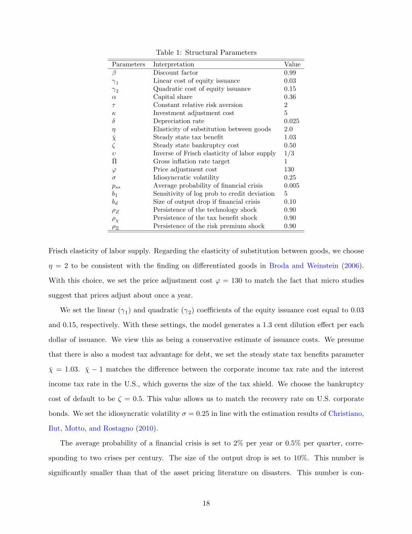
Table 1: Structural Parameters
Parameters Interpretation Valueβ Discount factor 0.99γ1 Linear cost of equity issuance 0.03γ2 Quadratic cost of equity issuance 0.15α Capital share 0.36τ Constant relative risk aversion 2κ Investment adjustment cost 5δ Depreciation rate 0.025η Elasticity of substitution between goods 2.0χ Steady state tax benefit 1.03ζ Steady state bankruptcy cost 0.50υ Inverse of Frisch elasticity of labor supply 1/3Π Gross inflation rate target 1ϕ Price adjustment cost 130σ Idiosyncratic volatility 0.25pss Average probability of financial crisis 0.005b1 Sensitivity of log prob to credit deviation 5bd Size of output drop if financial crisis 0.10ρZ Persistence of the technology shock 0.90ρχ Persistence of the tax benefit shock 0.90ρΞ Persistence of the risk premium shock 0.90
Frisch elasticity of labor supply. Regarding the elasticity of substitution between goods, we choose
η = 2 to be consistent with the finding on differentiated goods in Broda and Weinstein (2006).
With this choice, we set the price adjustment cost ϕ = 130 to match the fact that micro studies
suggest that prices adjust about once a year.
We set the linear (γ1) and quadratic (γ2) coefficients of the equity issuance cost equal to 0.03
and 0.15, respectively. With these settings, the model generates a 1.3 cent dilution effect per each
dollar of issuance. We view this as being a conservative estimate of issuance costs. We presume
that there is also a modest tax advantage for debt, we set the steady state tax benefits parameter
χ = 1.03. χ − 1 matches the difference between the corporate income tax rate and the interest
income tax rate in the U.S., which governs the size of the tax shield. We choose the bankruptcy
cost of default to be ζ = 0.5. This value allows us to match the recovery rate on U.S. corporate
bonds. We set the idiosyncratic volatility σ = 0.25 in line with the estimation results of Christiano,
Ilut, Motto, and Rostagno (2010).
The average probability of a financial crisis is set to 2% per year or 0.5% per quarter, corre-
sponding to two crises per century. The size of the output drop is set to 10%. This number is
significantly smaller than that of the asset pricing literature on disasters. This number is con-
18

sistent, for instance, with the recent US experience (and conservative relative to other countries’
experience). The sensitivity of the financial crisis probability to excess credit is 5, so that a 20%
increase in inefficient credit doubles the probability of financial crisis. We study extensively the
sensitivity of our results to these parameters below.
Regarding the aggregate shock processes, we take an agnostic approach and set all the persis-
tence parameters equal to 0.9. We then calibrate the standard deviation of technology shock equal
to 0.01. We then choose the other two shock volatilities such that the variance decomposition share
of output can be allocated to technology shock, demand shock and financial shock with 40-40-20
shares, respectively.
4.2 Model Properties With a Standard Policy Rule
As a first step, we illustrate how our model economy behaves in response to the three fundamental
impulses that we consider - a productivity shock, an aggregate demand shock, and the financial
shock. To solve the model, we assume an inertial Taylor (1999) rule:
Rt = 0.85×Rt−1 + 0.15× (R∗ + 1.5× (πt − π∗) + yt) ,
where yt is the output gap11, and πt is the year-over-year inflation rate. We summarize the main
mechanisms in the model by explaining what happens to output, inflation, debt, the policy rate,
and the probability of a crisis. As a further diagnostic we also report the effect that a shock to the
policy rule has on the same variables.
A productivity shock, shown in Figure 1, leads to higher output and lower inflation as is common
in New Keynesian models. The policy rule leads the central bank to cut the policy rate but not
sufficiently to stabilize inflation or to allow output to rise in line with potential. Put differently,
lower inflation reflects the decline in current and future marginal costs that arise from higher
productivity and the fact that monetary policy does not bring demand in line with this higher
supply.
The output surge leads to higher borrowing to finance investment, but because output does not
keep up with growth in potential, credit actually rises less than in the frictionless benchmark. As a
11We define this gap to be the difference between the level of output and the one that would prevail in an economywithout nominal rigidities and without financial shocks.
19

Figure 1: Impulse Response to Productivity Shock: Baseline
0 10 20 30
%
0
0.1
0.2
0.3
0.4
0.5(a) Output
0 10 20 30-0.14
-0.12
-0.1
-0.08
-0.06
-0.04
-0.02
0(b) Inflation
0 10 20 300.2
0.22
0.24
0.26
0.28
0.3
0.32
0.34(c) Debt
Quarters0 10 20 30
Ppt
(an
nual
ized
)
-0.05
-0.04
-0.03
-0.02
-0.01
0(d) Probability of Crisis
Quarters0 10 20 30
-0.18
-0.16
-0.14
-0.12
-0.1
-0.08
-0.06
-0.04(e) Policy Rate
result, the probability of crisis falls modestly (by 4 basis points, so that the probability drops from
2% per year to 1.96%).
The response to a demand shock (modeled following Smets and Wouters (2007) as a change
in agents’ discount rate for nominal bond), shown in Figure 2, leads to lower output and inflation
(given the assumed interest rate rule). The lower output in turn leads to lower debt and lower risk
of financial crisis.
Next, in Figure 3, we show the effect of a financial shock, which reflects an inefficient shock to
credit supply. This type of shock leads to a large expansion of credit which reduces the user cost of
capital and leads to a boom in investment and, to a lesser extent, also in output. The lower user
cost feeds through to lower inflation. The spike in debt (that is permitted with this policy rule)
significantly increases the risk of financial crisis, from 2% per year to 2.28% per year.
Finally we illustrate how a “monetary shock” affects this model economy. Although we most
interested in optimal monetary policy rules, showing the impact of deviation from the rule is
informative about two aspects of the model. Figure 4 displays the responses of our main variables
to a 100 basis point (1%) increase in the (annualized) policy rate. One important takeway from
20

Figure 2: Impulse Response to Demand Shock: Baseline
0 10 20 30
%
-1
-0.8
-0.6
-0.4
-0.2
0(a) Output
0 10 20 30-0.4
-0.3
-0.2
-0.1
0
0.1(b) Inflation
0 10 20 30-1.4
-1.2
-1
-0.8
-0.6
-0.4
-0.2
0(c) Debt
Quarters0 10 20 30
Ppt
(an
nual
ized
)
-0.14
-0.12
-0.1
-0.08
-0.06
-0.04
-0.02
0(d) Probability of Crisis
Quarters0 10 20 30
-0.5
-0.4
-0.3
-0.2
-0.1
0(e) Policy Rate
Figure 3: Impulse Response to Financial Shock: Baseline
0 10 20 30
%
-0.1
-0.05
0
0.05
0.1
0.15
0.2
0.25(a) Output
0 10 20 30-0.25
-0.2
-0.15
-0.1
-0.05(b) Inflation
0 10 20 300
0.5
1
1.5
2
2.5
3(c) Debt
Quarters0 10 20 30
Ppt
(an
nual
ized
)
0
0.05
0.1
0.15
0.2
0.25
0.3(d) Probability of Crisis
Quarters0 10 20 30
-0.12
-0.1
-0.08
-0.06
-0.04
-0.02(e) Policy Rate
21

Figure 4: Impulse Response to Monetary Policy Shock: Baseline
0 10 20 30
%
-0.6
-0.5
-0.4
-0.3
-0.2
-0.1
0
0.1(a) Output
0 10 20 30-0.2
-0.15
-0.1
-0.05
0
0.05(b) Inflation
0 10 20 30-1
-0.8
-0.6
-0.4
-0.2
0(c) Debt
Quarters0 10 20 30
Ppt
(an
nual
ized
)
-0.1
-0.08
-0.06
-0.04
-0.02
0(d) Probability of Crisis
Quarters0 10 20 30
0
0.2
0.4
0.6
0.8
1(e) Policy Rate
the figure is that the shock leads to a decline in output and inflation.12 The output drop leads
to a decline of credit and hence the probability of crisis. The second important conclusion from
this exercise is that the sensitivity of the risk of crisis to an increase in the policy rate is by no
means extreme - this fairly large monetary shock only generates on impact a reduction of 8 basis
points in the annual probability of crisis, i.e. moving it from 2% to 1.92%. This is magnitude
of the change is consistent with the empirical estimates reviewed by IMF (2015). We share the
view of IMF (2015) that these estimates are somewhat uncertain, but it is important to note that
our subsequent conclusions about the desirability of leaning against the wind are not driven by a
presumption that monetary policy has powerful effects on the risk of a crisis.
12Our model does not generate hump-shapes in response to this shock because it lacks some of the propagationmechanisms introduced by Christiano Eichenbaum and Evans (2005) or Smets and Wouters (2007) such as inflationindexation or consumer habits. We believe this is not critical for our results.
22

5 Optimal simple rules
Having established the basic model properties, we consider policy rules that specify the interest
rate as a function of last period’s interest rate, inflation, the output gap and/or the “credit gap”,
i.e. Bt/Bft , the deviation of credit from the level that would prevail with only productivity shocks
and flexible prices. Past research have shown such rules typically perform well in models like ours.
Because real time measurement of the output and credit gaps is difficult,13 we also study rules that
rely on imperfectly measured version of these variables, namely deviations of output and credit
from their steady state values. Our goal is to establish the conditions when responding to credit
may be beneficial. The benchmark for comparisons is the welfare of a representative consumer who
cares not only about the usual fluctuations in output and inflation, but also about risks that bring
large persistent drops in output and consumption. As we will see, in some configurations of the
model the central bank finds it optimal to respond to credit so as to smooth the risk of financial
crisis, even though this leads to higher output and inflation volatility.
Our main result is that leaning against the wind can be beneficial provided that three conditions
are met: (1) financial crises have important output effects; (2) financial shocks are important, i.e.
the variance of the financial shocks and the associated swing in inefficient credit are large enough,
and (3) financial crises are endogenous, i.e. they are caused in part by inefficient credit. In
contrast, if there are no financial shocks, even with other financial imperfections present, we obtain
the standard result that stabilizing inflation is a sufficient condition for maximizing welfare. In this
latter case, a simple Taylor rule that puts enough weight on the output gap can maximize welfare.
In the absence of price markup shock, so called divine coincidence holds, and the same outcome can
be achieved by maximizing the inflation coefficient in this case. If there are financial shocks, but
financial crises are exogenous, a simple rule that puts weight on the output gap still outperforms
credit-based rules, because targeting the output gap is a more direct way to eliminate undesirable
fluctuations in output and inflation.
Obviously, these results depend on parameter choices. For instance, it is clear that if financial
crises have small effects, or the variance of financial shocks is small, responding to output may still be
preferable to responding to credit. In the results that follow we have calibrated the financial shocks
13See Orphanides and Williams (2002) and Edge and Meisenzahl (2011).
23

so that they account for a bit less than 20% of the variance of output, and demand and productivity
shocks equally account for the remainder (i.e., 40% each). We discuss some robustness exercises
after we introduce our main findings. However, because we have not estimated the model and we
view these results as being indicative rather than dispositive. Put differently, rather than giving
a definitive answer to the question of whether leaning against the wind is desirable, we think our
framework is useful precisely because it permits us to understand, within a fairly standard DSGE
model, which parameters and model features govern whether responding to credit conditions is
beneficial.
5.1 Methodology
We consider policy rules of the following form:
Rt = ρRt−1 + (1− ρ)(R∗ + φπ(πt − π∗) + φyyt + φbbt)
where πt is again the year-over-year inflation rate, yt is the output gap and bt is the credit gap,
i.e. log(Bt/B
ft
). Note that bt is the variable which determines the probability of a financial crisis,
according to (21). Throughout this exercise we set ρ = 0.85 and φπ = 1.5. Our motivation for
imposing these restrictions is to make analysis transparent, and to require that the policy rule
to resemble the kind that broadly describes actual central bank decisions. We then consider the
welfare consequences of policy rules with different coefficients for φy or φb. Specifically, we rank
rules according to the expected utility they provide to the representative consumer and find the
value of φy and/or φb that maximizes this expected utility.14,15 We first consider the simple case
where only one gap matters so that φb = 0 or φy = 0. We then discuss results when we optimize
over φb and φy jointly.
14In contrast, many papers maximize a quadratic loss function of inflation and unemployment. In our case thisapproach would not capture the cost of financial crises, which permanently lower productivity. It is also a prioriattractive to use a micro-founded welfare criterion.
15In practice, we first rewrite the system of equations that determines the equilibrium around the stochas-tic trend induced by disaster. This system can then be solved using standard perturbation methods sinceit has no jumps. We then use a second-order approximation of the utility. See appendix for details, andhttps://sites.google.com/site/fgourio/ for the code used to solve the paper (to be posted).
24
5.2 Main Result
Table 2 summarizes the outcomes that lead to our main conclusion. When we select the best rule
that depends solely on a correctly measured output gap, the optimal sensitivity is very high16,
around 100, so that monetary policy eliminates all inefficient fluctuations of output. As can be
seen, this monetary policy rule generates also a relatively small volatility of inflation. When this
rule is followed, crises occur about 2.08 percent of the time, though the standard deviation of the
probability of crises is 0.61 percent, so households face the risk that crises can be more frequent
than that.
When we select the best rule that depends solely on the correctly measured credit gap, we
obtain a coefficient of 1.88 on the credit gap. This rule generates significantly greater volatility
of output and inflation than the one based on the output gap.17 Yet, the credit-gap based rule
outperforms the output-gap based rule in terms of welfare. The difference in utility is equivalent
to a permanent increase of consumption of 0.06%, a small but significant number. In all of the
comparisons that follow, we report the consumption equivalent change between a rule based only
on the output gap and those that depend on the credit gap or both gaps; by this convention, the
consumption equivalent for the rule that focusing on output gap only is always zero.
The gain in welfare occurs because the LAW policy is sacrificing volatility in order to limit the
financial crisis risk: the probability of a financial crisis is now both smaller and substantially less
volatile. The reduction in the mean probability of crisis is driven, in part, by the functional form
we use to insure that the crisis probability lies between zero and one.18 While this effect may seem
at first mechanical, it reflects the real constraint that financial crisis probability is bounded below
(by zero). As such, decreasing the volatility of financial crisis leads to lower mean because the mean
is driven by the occasional upswings.
Figure 5 depicts the response of macroeconomic aggregates to the three fundamental shocks
under the standard Taylor (the solid blue line), the rule that responds using only the output gap
(the dashed red line), and the rule that responds using only the credit gap (the dotted green line).
Our main conclusion is best understood by comparing what the different rules imply about policy
16We set an upper bound of 100, and a lower bound of 0, to ensure that the optimization problem well-posed.Allowing for values higher than 100 does not materially alter the results.
17The output volatility measure does not take into account financial crises.18We specify a process for the log of the probability and that implies that lower volatility also brings a lower mean.
25
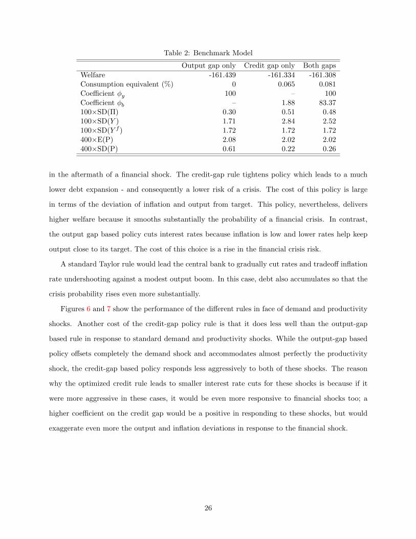
Table 2: Benchmark Model
Output gap only Credit gap only Both gaps
Welfare -161.439 -161.334 -161.308Consumption equivalent (%) 0 0.065 0.081Coefficient φy 100 – 100
Coefficient φb – 1.88 83.37100×SD(Π) 0.30 0.51 0.48100×SD(Y ) 1.71 2.84 2.52100×SD(Y f ) 1.72 1.72 1.72400×E(P) 2.08 2.02 2.02400×SD(P) 0.61 0.22 0.26
in the aftermath of a financial shock. The credit-gap rule tightens policy which leads to a much
lower debt expansion - and consequently a lower risk of a crisis. The cost of this policy is large
in terms of the deviation of inflation and output from target. This policy, nevertheless, delivers
higher welfare because it smooths substantially the probability of a financial crisis. In contrast,
the output gap based policy cuts interest rates because inflation is low and lower rates help keep
output close to its target. The cost of this choice is a rise in the financial crisis risk.
A standard Taylor rule would lead the central bank to gradually cut rates and tradeoff inflation
rate undershooting against a modest output boom. In this case, debt also accumulates so that the
crisis probability rises even more substantially.
Figures 6 and 7 show the performance of the different rules in face of demand and productivity
shocks. Another cost of the credit-gap policy rule is that it does less well than the output-gap
based rule in response to standard demand and productivity shocks. While the output-gap based
policy offsets completely the demand shock and accommodates almost perfectly the productivity
shock, the credit-gap based policy responds less aggressively to both of these shocks. The reason
why the optimized credit rule leads to smaller interest rate cuts for these shocks is because if it
were more aggressive in these cases, it would be even more responsive to financial shocks too; a
higher coefficient on the credit gap would be a positive in responding to these shocks, but would
exaggerate even more the output and inflation deviations in response to the financial shock.
26

Figure 5: Impulse Response to Financial Shock: Optimal Simple Rule
10 20 30
%
-2
-1.5
-1
-0.5
0
(a) Output
Taylor Rule
Output Gap
Credit Gap
10 20 30
-1.5
-1
-0.5
0(b) Inflation
10 20 300
1
2
3
4
5
(c) Debt
Quarters10 20 30
Ppt
(an
nual
ized
)
0
0.1
0.2
0.3
0.4
0.5
(d) Probability of Crisis
Quarters10 20 30
-1
-0.5
0
(e) Policy Rate
Figure 6: Impulse Response to Demand Shock: Optimal Simple Rule
10 20 30
%
-0.8
-0.6
-0.4
-0.2
0(a) Output
Taylor Rule
Output Gap
Credit Gap
10 20 30-0.3
-0.25
-0.2
-0.15
-0.1
-0.05
0
(b) Inflation
10 20 30
-1.2
-1
-0.8
-0.6
-0.4
-0.2
0(c) Debt
Quarters10 20 30
Ppt
(an
nual
ized
)
-0.12
-0.1
-0.08
-0.06
-0.04
-0.02
0(d) Probability of Crisis
Quarters10 20 30
-1
-0.8
-0.6
-0.4
-0.2
0(e) Policy Rate
27

Figure 7: Impulse Response to Technology Shock: Optimal Simple Rule
10 20 30
%
0
0.1
0.2
0.3
0.4
0.5
0.6
(a) Output
Taylor Rule
Output Gap
Credit Gap
10 20 30
-0.12
-0.1
-0.08
-0.06
-0.04
-0.02
0(b) Inflation
10 20 300
0.1
0.2
0.3
0.4
0.5
0.6
(c) Debt
Quarters10 20 30
Ppt
(an
nual
ized
)
-0.04
-0.03
-0.02
-0.01
0
(d) Probability of Crisis
Quarters10 20 30
-0.4
-0.3
-0.2
-0.1
0(e) Policy Rate
5.3 Understanding the result
To confirm the interpretation that we have offered for the main findings, it is instructive to shutdown
various features of the model to see how they change the results. A particularly helpful experiment
is to turn off the financial shocks (i.e. set σχ = 0) and make the financial crises exogenous events
(e.g. b1 = 0). The environment then amounts to a standard New Keynesian model that includes a
debt-equity tradeoff in capital structure and exogenous crises. The main findings are summarized
in Table 3. In this environment, a policy that responds enough to either the output or credit gap
can essentially perfectly stabilize inflation. After a demand shock, monetary policy offsets the shock
to fully stabilize output and inflation. On the other hand, when a productivity shock occurs, the
policy keeps inflation on target and lets output respond fully to the shock. This result is standard
in New Keynesian models - the divine coincidence property (Blanchard and Gali (2007)) applies
and so there is no trade-off between output and inflation volatility, and this optimal policy can be
(approximately) implemented by either simple rule provided they are sufficiently aggressive.19
19Note that there is no intrinsic reason as to why one simple rule should perform better than the other in terms ofwelfare in this case. Also note that output and inflation volatility as well as mean and standard deviation of financialcrisis probability are quite close.
28

Table 3: No Financial Shocks, Exogenous Financial Crises
Output gap only Credit gap only Both gaps
Welfare -161.023 -160.989 -160.989Consumption equivalent (%) 0 0.021 0.021Coefficient φy 100 – 0
Coefficient φb – 95.78 95.78100×SD(Π) 0.01 0.01 0.01100×SD(Y ) 1.71 1.67 1.66100×SD(Y f ) 1.72 1.72 1.72400×E(P) 2 2 2400×SD(P) 0 0 0
Table 4: No Financial Shocks, Endogenous Financial Crises
Output gap only Credit gap only Both gaps
Welfare -160.985 -160.988 -160.985Consumption equivalent (%) 0 -0.002 0Coefficient φy 100 – 100
Coefficient φb – 96.1 0100×SD(Π) 0.01 0.01 0.01100×SD(Y ) 1.71 1.66 1.71100×SD(Y f ) 1.72 1.72 1.72400×E(P) 1.99 2.00 1.99400×SD(P) 0.01 0.01 0.01
To further build intuition, we now relax the assumption of exogenous financial crises. The
main results are reported in Table 4. The findings are nearly identical to the prior case. This
is because there is no reason to offset the credit fluctuations driven by the productivity shock,
which are efficient and do not contribute to financial risk. As for demand shocks, the credit
fluctuations they create are actually eliminated once output volatility is eliminated. Hence, there
is no trade-off between credit stabilization and output/inflation stabilization, and the same policies
as in the previous case can implement an efficient allocation without creating any inefficient credit
movements.
As a third point of comparison, we now reintroduce financial shocks, though we now suppose
that crises are exogenous. In this version of the model both rules continue to perform about as
well. The main findings are summarized in Table 5. The novelty compared to the previous cases
is that the response to the output gap is diminished. This occurs because the response that would
be required to offset demand and productivity shocks is not consistent with the response needed
to respond to the financial shock. But the credit gap rule suffers from the same issue and has to
29
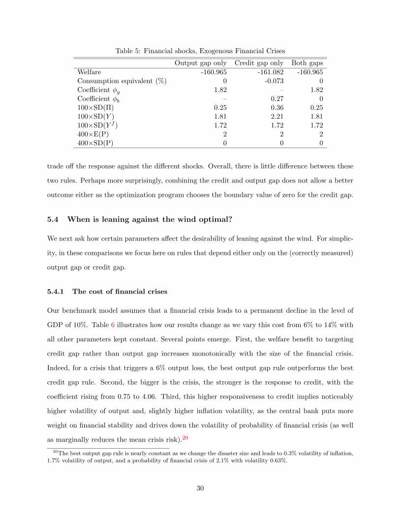
Table 5: Financial shocks, Exogenous Financial Crises
Output gap only Credit gap only Both gaps
Welfare -160.965 -161.082 -160.965Consumption equivalent (%) 0 -0.073 0Coefficient φy 1.82 – 1.82
Coefficient φb – 0.27 0100×SD(Π) 0.25 0.36 0.25100×SD(Y ) 1.81 2.21 1.81100×SD(Y f ) 1.72 1.72 1.72400×E(P) 2 2 2400×SD(P) 0 0 0
trade off the response against the different shocks. Overall, there is little difference between these
two rules. Perhaps more surprisingly, combining the credit and output gap does not allow a better
outcome either as the optimization program chooses the boundary value of zero for the credit gap.
5.4 When is leaning against the wind optimal?
We next ask how certain parameters affect the desirability of leaning against the wind. For simplic-
ity, in these comparisons we focus here on rules that depend either only on the (correctly measured)
output gap or credit gap.
5.4.1 The cost of financial crises
Our benchmark model assumes that a financial crisis leads to a permanent decline in the level of
GDP of 10%. Table 6 illustrates how our results change as we vary this cost from 6% to 14% with
all other parameters kept constant. Several points emerge. First, the welfare benefit to targeting
credit gap rather than output gap increases monotonically with the size of the financial crisis.
Indeed, for a crisis that triggers a 6% output loss, the best output gap rule outperforms the best
credit gap rule. Second, the bigger is the crisis, the stronger is the response to credit, with the
coefficient rising from 0.75 to 4.06. Third, this higher responsiveness to credit implies noticeably
higher volatility of output and, slightly higher inflation volatility, as the central bank puts more
weight on financial stability and drives down the volatility of probability of financial crisis (as well
as marginally reduces the mean crisis risk).20
20The best output gap rule is nearly constant as we change the disaster size and leads to 0.3% volatility of inflation,1.7% volatility of output, and a probability of financial crisis of 2.1% with volatility 0.63%.
30

Table 6: Effect of Financial Crisis Size on Optimal Credit Policy
Financial crisis size ( bc) 6% 8% 10% 12% 14%(benchmark)
Optimal coeff. on credit φb 0.75 1.17 1.88 2.88 4.06Welfare difference -0.010 0.038 0.105 0.191 0.295Consumption equivalent (%) -0.006 0.023 0.065 0.118 0.182SD(Y) under LAW 2.36 2.59 2.85 3.05 3.20SD(π) under LAW 0.45 0.48 0.51 0.53 0.54Mean(P) under LAW 2.05 2.03 2.02 2.01 2.00SD(P) under LAW 0.40 0.31 0.22 0.16 0.13
Table 7: Effect of Sensitivity of Crisis to Excess Credit on Optimal Policies
Sensitivity of crisis to excess credit ( b1) 2 3 5 7 8(benchmark)
Optimal coeff. on credit φb 0.30 0.46 1.88 5.41 7.70Welfare difference -0.089 -0.059 0.105 0.491 0.751Consumption equivalent (%) -0.055 -0.036 0.065 0.303 0.463SD(Y) under LAW 2.20 2.21 2.85 3.28 3.38SD(π) under LAW 0.37 0.41 0.51 0.54 0.55Mean(P) under LAW 2.01 2.02 2.02 2.0 2.00SD(P) under LAW 0.25 0.31 0.22 0.14 0.12
5.4.2 The sensitivity of crises to excess credit
A key parameter for our results is how much excess credit matters for financial crises, represented
by the coefficient b1. A large value of b1 means that excess credit has a strong effect on the risk of
crisis and hence on welfare. This naturally gives rise to a stronger motive to lean against excess
credit. Table 7 confirms this intuition. First, for low values of b1, LAW is outperformed by the
output gap rule. Second, the coefficient on credit optimally rises with b1. This allows to offset to
some extent the increase in the volatility of financial crisis probability that would otherwise occur
mechanically. Third, this policy is chosen despite a clear cost in terms of higher output and inflation
volatility.
5.4.3 The importance of financial shocks
Perhaps most basically, the magnitude of the (inefficient) financial shocks is critical for our results.
We already illustrated that if there are no financial shocks, leaning against the wind brings essen-
tially no benefits relative to standard policies. Table 8 provides more details on the importance of
this consideration. Here too, we see that the welfare difference between the best credit gap policy
31

Table 8: Effect of Standard Deviation of Financial Shocks on Optimal Policy
Standard dev. of financial shocks 33% 66% 100% 133% 166%(relative to benchmark) (benchmark)
Optimal coeff. on credit φb 96.1 2.96 1.88 1.55 1.41Welfare difference LAW-OG 0.004 0.037 0.105 0.205 0.336Consumption equivalent (%) 0.002 0.022 0.065 0.126 0.207SD(Y) under LAW 1.97 2.38 2.85 3.34 3.87SD(π) under LAW 0.19 0.36 0.51 0.65 0.81Mean(P) under LAW 2.00 2.00 2.02 2.04 2.08SD(P) under LAW 0.7 0.13 0.22 0.31 0.40
and the best output gap policy is increasing in the variance of financial shocks. The effects on
output and inflation volatility as well as the financial crisis probability are more subtle because
they result both from (i) the higher variance of financial shocks and (ii) the change in policy rule
in response to this higher variance.
5.4.4 The role of risk aversion
We next explore how the willingness of households to bear macroeconomic risk affects our results.
On one side, higher risk aversion makes agents more fearful of financial crises. On the other hand,
higher risk aversion also makes agents less willing to tolerate the higher business cycle volatility
implied by LAW. Moreover, with expected utility preferences, a higher risk aversion implies a lower
elasticity of substitution, which affects the response of the economy to monetary policy (as well as
the dynamics of the model more generally). Table 9 reveals that the first effect seems to dominate
- the higher the risk aversion, the larger the benefits from leaning against the wind. With a risk
aversion of 0.5, an output-gap rule outperforms a credit-gap rule, but the benefits of using the
credit gap rule rise with risk aversion. The optimal policy largely stabilizes fluctuations in financial
crisis risk.
Figure 8 summarizes many of the central findings of the paper. On the horizontal axis, we vary
the size of the financial crisis. On the vertical axis we vary risk aversion. The lines that are drawn
trace out isoquants in units of equivalent consumption between the best LAW policy (that responds
only to the credit gap on top of inflation) and the best monetary policy rule that responds only
to the output gap (on top of inflation).21 The zero consumption equivalence curve traces out all
21Each policy is optimized with respect to the coefficient on the credit gap or output gap, as in the exercises above.
32

Figure 8: Welfare Gain from LAW: the Effects of Risk Aversion and the Size of Financial Crisis
-0.5-0.4
-0.4
-0.3-0.3
-0.3
-0.2-0.2
-0.2
-0.1
-0.1-0.1
0
0
0
0
0.1
0.1
0.1
0.20.2
0.3
0.3
0.40.5
2 4 6 8 10 12 14
Financial crisis size (%)
0.5
1
1.5
2
2.5
3
3.5
4
4.5
5
Ris
k A
vers
ion
the combination of the size of the crisis and the representative household’s level of risk aversion
where the two policies deliver equivalent welfare. Points to the right and above the zero curve show
the regions where LAW delivers higher welfare and below and to the left show combinations where
the output gap rule performs better. In the benchmark model, described in Table 2 with risk
aversion of two and a crisis that brings a permanent ten percent output loss, LAW is better. The
results from Table 6 described how welfare varied when we fixed risk aversion at two and varied
the size of the crisis. This figure fills in the rest of the parameter space. Not surprisingly, as risk
aversion rises, LAW’s relative performance improves. For instance, if risk aversion is three, then
LAW is the preferred policy even for a crisis that involves a one-time output loss of as little as five
percent. Conversely, if risk aversion is much lower, say one, then even a crisis that drops output
by 14 percent is not enough to justify a LAW policy.
5.5 Trading off financial stability vs. macroeconomic stability
Our model results demonstrate a significant trade-off between the traditional mandates of monetary
policy - output and inflation stability - and financial stability - stabilizing, and if possible reducing
33

Table 9: Risk Aversion and Leaning Against the Wind
CRRA 0.5 1.5 2 3 4(benchmark)
Optimal coeff. on credit φb 87.67 1.15 1.88 6.61 97.72Welfare difference LAW-OG -0.214 0.032 0.105 0.273 0.514Consumption equivalent (%) -0.33 0.02 0.06 0.12 0.17SD(Y) under LAW 5.00 2.99 2.85 2.70 2.53SD(π) under LAW 0.64 0.48 0.51 0.54 0.55Mean(P) under LAW 2.00 2.02 2.02 2.00 2.00SD(P) under LAW 0.01 0.31 0.22 0.09 0.01
the probability of financial crisis. To illustrate this trade-off, we consider a range of values for φb
and trace out the frontiers that exist among welfare, volatility of output, volatility of inflation rate,
mean and volatility of probability of financial crisis. The policy maker can choose a point on these
frontiers - a particular rule - depending on the weights she puts on the relative volatilities.
In our case, the frontiers are somewhat more complex, because there are more than two objec-
tives. Figure 9 is an attempt at illustrating these trade-offs. The blue line depicts the outcomes in
our benchmark model as we vary the coefficient on the credit gap. (The zero weight on credit is the
leftmost end point of each line.) The red line depicts the same frontier as we change a parameter:
the left column depicts the case for a lower sensitivity of financial crisis to credit (b1); the middle
column shows the frontier in the case of a smaller output decline should a financial crisis occur;
and the right column shows the effect of changing the variance of financial shocks.
The figure shows that policies that respond weakly to credit (left side of plots) generate lower
inflation volatility but much higher volatility of the probability of financial crisis, and slightly higher
mean crisis risk, generating a clear trade-off. The effect on output volatility is U-shaped as a small
response on credit can eliminate some undesirable output fluctuations due to demand shocks, but
much stronger ones generate excessive output fluctuations (as we saw earlier). When the sensitivity
b1 is lowered, the frontier flattens as the trade-off between financial stability and inflation volatility
becomes much less acute. Similarly, when the losses from a financial crisis are smaller the trade-off
becomes flatter. A lower variance of financial shocks similarly shifts the frontier to higher welfare,
and a lower volatility of the financial crisis probability.
34

Figure 9: Tradingoff of Leaning Against the Wind
0.3 0.4 0.5 0.6
Wel
fare
-162.5
-162
-161.5
-161Lower sensitivity b1
0.3 0.4 0.5 0.6-164
-162
-160
-158 Smaller fin crisis size
0.2 0.4 0.6-162.5
-162
-161.5
-161 Lower var of fin shocks
0.3 0.4 0.5 0.6
400*
Mea
n(P
)
2
2.2
2.4
0.3 0.4 0.5 0.62
2.2
2.4
0.2 0.4 0.62
2.2
2.4
0.3 0.4 0.5 0.6
400*
SD
(P)
0
0.5
1
1.5
0.3 0.4 0.5 0.60
0.5
1
1.5
0.2 0.4 0.60
0.5
1
1.5
100*SD(:)0.3 0.4 0.5 0.6
100*
SD
(Y)
0.02
0.03
0.04
100*SD(:)0.3 0.4 0.5 0.6
0.02
0.03
0.04
100*SD(:)0.2 0.4 0.6
0.02
0.03
0.04
5.6 Mismeasurement
Finally, an important practical consideration is that neither the output gap nor the credit gap is
actually observable. The importance of inefficient credit fluctuations depends on several factors.
One is the size of the financial shocks, but the observed level of borrowing depends also on changes
in fundamental financing needs that come from technology shocks. In our baseline, there are no
other fundamental reasons why credit varies. In reality, deregulation, changes in property rights
and many other factors could lead to a benign surge in credit and a central bank would need to be
able to separate those swings from the inefficient ones.
To quantify this, we search again for the best policy rules in our baseline specification where the
central bank is restricted to just observing actual output and credit - that is, it uses the deviation
from the steady-state rather than the deviation from the efficient benchmark. The results are
shown in Table 9 (and these should be compared to the findings in Table 2). The output gap rule
35

Table 10: Optimal Policy Rules with Mismeasured Gaps
Output gap only Credit gap only Both gaps
Welfare -161.646 -161.426 -161.426Consumption equivalent (%) 0 0.124 0.124Coefficient φy 100 0 0.02
Coefficient φb 0 1.59 1.61100×SD(Π) 0.39 0.53 0.53100×SD(Y ) 0.00 2.41 2.40100×SD(Y f ) 1.72 1.72400×E(P) 2.09 2.01 2.01400×SD(P) 0.70 0.34 0.34
now eliminates all fluctuations in output, including the efficient fluctuations. This leads to higher
inflation volatility and noticeably lower welfare. Relying on the mismeasured credit gap still leads
to a similar tradeoff as in the baseline model. The central bank delivers less frequent and less
volatile crises, in exchange for higher inflation and output volatility. The relative performance of
the rule based on mismeasured credit is bigger in this scenario than in the one with both gaps are
perfectly measured. In fact, the best rule when both gaps are considered puts almost no weight on
the output gap (and the welfare is about the same as when only the credit gap is used).
The welfare level is actually slightly higher when the mismeasured credit gap is used instead
of the perfectly measured output gap; this conclusion depends on all the foregoing factors that
have been shown to determine the relative attractiveness of leaning against the wind. For instance,
in parameter configurations where the gains from leaning against the wind are low to begin with,
then tying the policy rate to mismeasured credit gap would not necessarily lead to higher welfare
than a rule that can be set based on a perfectly measured output gap. In these cases, however, the
mismeasured credit gap rule would still outperform the mismeasured output gap rule.
6 Conclusion
Conventional discussions about the links between monetary policy and financial stability typically
start by saying that one can appeal to different tools for different jobs. Macro-prudential regulation
can address stability concerns, while monetary policy can attend to managing inflation. We agree
that this would be the ideal arrangement, however, in practice in many countries this is easier said
than done. Macro-prudential policymaking is in its infancy and for some countries the tools barely
36

exist. These practical concerns motivate our analysis.
On the question of whether central banks should alter monetary policy to contain financial
stability risks IMF staff study (IMF (2015)) says “Based on our current knowledge, and in present
circumstances, the answer is generally no.” We believe this conclusion is too strong.
The model we have presented is highly stylized and the parameters are not estimated. Nonethe-
less, we believe it does capture the ingredients that many of the advocates of leaning against the
wind believe support the case for doing so. In particular, the model presumes that financial crises
are very costly, and are partly driven by credit conditions which monetary policy can affect. The
fact that the model can easily uncover circumstances where leaning against the wind is welfare
improving is, therefore, not surprising.
The model points to a number of factors that will determine the efficacy of leaning against
the wind. Our main hesitation in endorsing the IMF staff study (IMF (2015)) conclusion is that
many of these factors are difficult to measure and our reading of existing empirical work is that we
still do not have much guidance about how to calibrate certain of these key elasticities. Perhaps
subsequent work will confirm the IMF conclusion but for now we believe it is too early to say that
the question is settled.
One powerful conclusion from the model is that the case for leaning against the wind likely
rests on accepting somewhat higher volatility of inflation and output, in exchange for smoothing
out the risk of crises. If central banks are going to embrace this policy, they will need to invest
substantially in explaining this tradeoff to the public and to legislatures.
37

References
Adrian, T., P. de Fontnouvelle, E. Yang, and A. Zlate (2015): “Macroprudential policy:case study from a tabletop exercise,” Staff Reports 742, Federal Reserve Bank of New York.
Ajello, A., T. Laubach, J. D. Lopez-Salido, and T. Nakata (2016): “Financial Stabilityand Optimal Interest-Rate Policy,” Finance and Economics Discussion Series 2016-067, Boardof Governors of the Federal Reserve System (U.S.).
Barro, R. J. (2006): “Rare Disasters and Asset Markets in the Twentieth Century,” The QuarterlyJournal of Economics, 121(3), 823–866.
(2009): “Rare Disasters, Asset Prices, and Welfare Costs,” American Economic Review,99(1), 243–64.
Bernanke, B. S., and M. Gertler (1999): “Monetary policy and asset price volatility,” Eco-nomic Review, (Q IV), 17–51.
Blanchard, O., and J. Gali (2007): “Real Wage Rigidities and the New Keynesian Model,”Journal of Money, Credit and Banking, 39, 35–65.
Broda, C., and D. E. Weinstein (2006): “Globalization and the Gains From Variety,” TheQuarterly Journal of Economics, 121(2), 541–585.
Cairo, I., and J. Sim (2016): “Income Inequality, Financial Crisis and Monetary Policy,” workingpaper, Federal Reserve Board.
Cerra, V., and S. C. Saxena (2008): “Growth Dynamics: The Myth of Economic Recovery,”American Economic Review, 98(1), 439–57.
Christiano, L. J., C. Ilut, R. Motto, and M. Rostagno (2010): “Monetary policy and stockmarket booms,” Proceedings - Economic Policy Symposium - Jackson Hole, pp. 85–145.
Dudley, W. C. (2015): “Is the Active Use of Macroprudential Tools Institutionally Realistic?,”Remarks by William C. Dudley, the President and Chief Executive Officer of the Federal ReserveBank of New York.
Edge, R. M., and R. R. Meisenzahl (2011): “The Unreliability of Credit-to-GDP Ratio Gapsin Real Time: Implications for Countercyclical Capital Buffers,” International Journal of CentralBanking, 7(4), 261–298.
Fisher, J. D. (2015): “On the Structural Interpretation of the SmetsWouters Risk PremiumShock,” Journal of Money, Credit and Banking, 47(2-3), 511–516.
Gabaix, X. (2011): “Disasterization: A Simple Way to Fix the Asset Pricing Properties of Macroe-conomic Models,” American Economic Review, 101(3), 406–09.
(2012): “Variable Rare Disasters: An Exactly Solved Framework for Ten Puzzles inMacro-Finance,” The Quarterly Journal of Economics, 127(2), 645–700.
Gertler, M., and P. Karadi (2011): “A model of unconventional monetary policy,” Journal ofMonetary Economics, 58(1), 17–34.
38

Gilchrist, S., and J. V. Leahy (2002): “Monetary policy and asset prices,” Journal of MonetaryEconomics, 49(1), 75–97.
Gourio, F. (2012): “Disaster Risk and Business Cycles,” American Economic Review, 102(6),2734–66.
(2013): “Credit Risk and Disaster Risk,” American Economic Journal: Macroeconomics,5(3), 1–34.
IMF (2015): “Monetary Policy and Financial Stability,” Discussion paper, International MonetaryFund.
Isor, M., and U. Szczerbowicz (2015): “Disaster Risk and Preference Shifts in a New KeynesianModel,” Working Papers 2015-16, CEPII research center.
Kumhof, M., R. Ranciere, and P. Winant (2015): “Inequality, Leverage, and Crises,” Amer-ican Economic Review, 105(3), 1217–45.
Lim, C. H., A. Costa, F. Columba, P. Kongsamut, A. Otani, M. Saiyid, T. Wezel, andX. Wu (2011): “Macroprudential Policy; What Instruments and How to Use them? LessonsFrom Country Experiences,” IMF Working Papers 11/238, International Monetary Fund.
Orphanides, A., and J. Williams (2002): “Robust Monetary Policy Rules with Unknown Nat-ural Rates,” Brookings Papers on Economic Activity, 33(2), 63–146.
Peek, J., E. S. Rosengren, and G. M. B. Tootell (2015): “Should US Monetary PolicyHave a Ternary Mandate?,” 59th economic conference: Macroprudential monetary policy, oct.2-3, 2015, the Federal Reserve Bank of Boston.
Reinhart, C. M., and K. S. Rogoff (2009): This Time Is Different: Eight Centuries of Finan-cial Folly, vol. 1 of Economics Books. Princeton University Press.
Schularick, M., and A. M. Taylor (2012): “Credit Booms Gone Bust: Monetary Policy,Leverage Cycles, and Financial Crises, 1870-2008,” American Economic Review, 102(2), 1029–61.
Smets, F. (2014): “Financial Stability and Monetary Policy: How Closely Interlinked?,” Interna-tional Journal of Central Banking, 10(2), 263–300.
Smets, F., and R. Wouters (2007): “Shocks and Frictions in US Business Cycles: A BayesianDSGE Approach,” American Economic Review, 97(3), 586–606.
Stein, J. C. (2013): “Overheating in Credit Markets: Origins, Measurement, and Policy Re-sponses,” Speech by Jeremy C. Stein, the Governor of the Federal Reserve System At the”Restoring Household Financial Stability after the Great Recession: Why Household BalanceSheets Matter”, research symposium sponsored by the Federal Reserve Bank of St. Louis, St.Louis, Missouri.
Svensson, L. E. (2016): “Cost-Benefit Analysis of Leaning Against the Wind: Are Costs LargerAlso with Less Effective Macroprudential Policy?,” NBER Working Papers 21902, National Bu-reau of Economic Research, Inc.
Taylor, J. B. (1999): “A Historical Analysis of Monetary Policy Rules,” in Monetary PolicyRules, NBER Chapters, pp. 319–348. National Bureau of Economic Research, Inc.
39

Tsai, J., and J. A. Wachter (2015): “Disaster Risk and its Implications for Asset Pricing,”NBER Working Papers 20926, National Bureau of Economic Research, Inc.
40
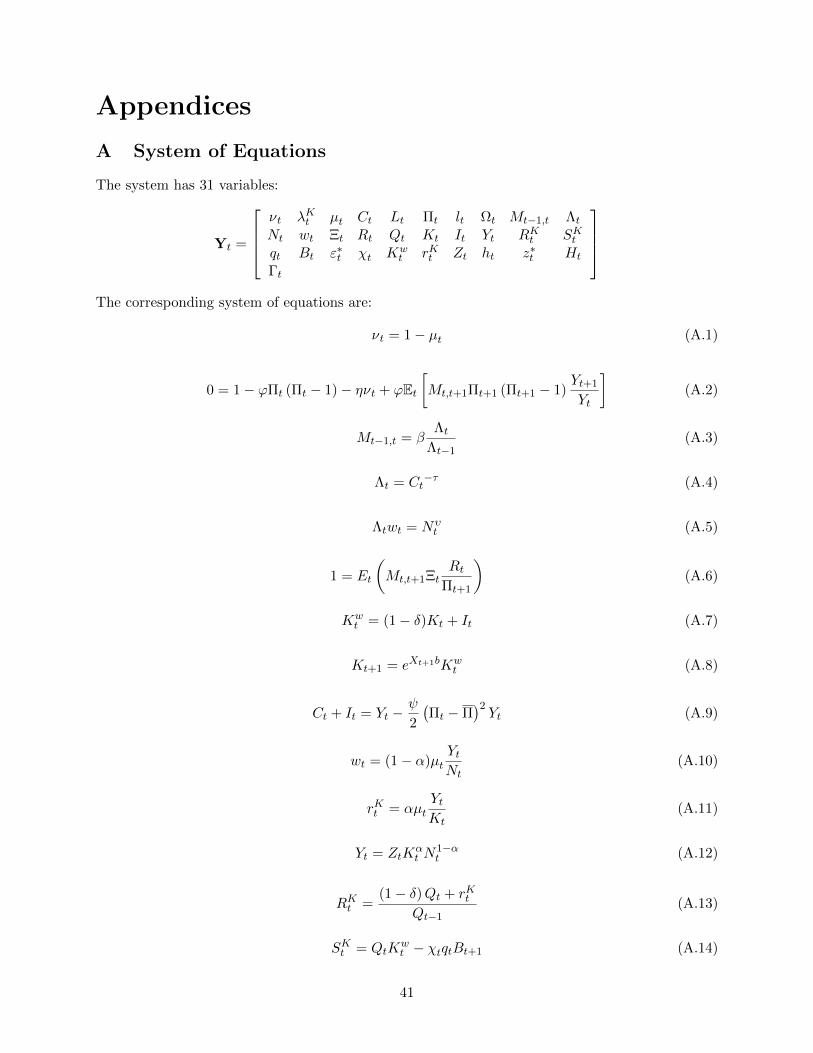
Appendices
A System of Equations
The system has 31 variables:
Yt =
νt λKt µt Ct Lt Πt lt Ωt Mt−1,t ΛtNt wt Ξt Rt Qt Kt It Yt RKt SKtqt Bt ε∗t χt Kw
t rKt Zt ht z∗t Ht
Γt
The corresponding system of equations are:
νt = 1− µt (A.1)
0 = 1− ϕΠt (Πt − 1)− ηνt + ϕEt[Mt,t+1Πt+1 (Πt+1 − 1)
Yt+1
Yt
](A.2)
Mt−1,t = βΛt
Λt−1(A.3)
Λt = Ct−τ (A.4)
Λtwt = Nυt (A.5)
1 = Et
(Mt,t+1Ξt
RtΠt+1
)(A.6)
Kwt = (1− δ)Kt + It (A.7)
Kt+1 = eXt+1bKwt (A.8)
Ct + It = Yt −ψ
2
(Πt −Π
)2Yt (A.9)
wt = (1− α)µtYtNt
(A.10)
rKt = αµtYtKt
(A.11)
Yt = ZtKαt N
1−αt (A.12)
RKt =(1− δ)Qt + rKt
Qt−1(A.13)
SKt = QtKwt − χtqtBt+1 (A.14)
41

ε∗t =Bt
RKt Qt−1Kt(A.15)
z∗t = σ−1(log ε∗t + 0.5σ2) (A.16)
Ht = Φ(z∗t ) (A.17)
ht = φ(z∗t ) (A.18)
Ωt = Φ(z∗t − σt) (A.19)
qt = Et
(Mt+1
(1−H(ε∗t+1) +
ζ
BtRKt+1QtKt+1Ω(ε∗t+1)
))(A.20)
Γt = Et(Mt+1R
Kt+1λ
Kt+1
)(A.21)
λKt = 1 + (χt − 1) ε∗t (1−H (ε∗t ))− (1− ζχt) Ω (ε∗t ) (A.22)
Γt = 1 + γ (1− χtL (lt)) (1− χtL (lt)) (A.23)
L (lt) = EtMt+1[Ω(ε∗t+1)ζRKt+1 + (1−H(ε∗t+1))ε∗t+1RKt+1] (A.24)
Et
Mt+1
(1−H
(ε∗t+1
)) [χt − 1
χt+ γ
(SKt
QtKt+1
)+ γ′
(SKt
QtKt+1
)](A.25)
= (1− ζ)Et
Mt+1ε
∗t+1h
(ε∗t+1
) [1 + γ
(SKt
QtKt+1
)+ γ′
(SKt
QtKt+1
)]
Qt = 1 + κ
(ItIt−1
− 1
)− Et
Mt,t+1
κ
2
[(It+1
It
)2
− 1
](A.26)
lt =Bt
QtKwt
(A.27)
logRt = (1− ρR) logRt−1 + ρR[logR+ ρΠ log(Πt/Π) + ρY log(Yt/YFt )] (A.28)
logχt = (1− ρχ) logχ+ ρχ logχt−1 + σχεχ,t (A.29)
Zt+1 = eXt+1beξt+1Zt (A.30)
log Ξt = (1− ρΞ) log Ξ + ρΞ log Ξt−1 + σΞεΞ,t (A.31)
42

B Detrending
Define Yt = Yt/Zt, Kt = Kt/Zt,etc. - we can then rewrite the system of equations:
Mt,t+1 = β
(Ct+1
Ct
)−σ (1−Nt+1
1−Nt
)υ(1−σ)
= β
(Ct+1
Ct
)−σ (Zt+1
Zt
)−σ (1−Nt+1
1−Nt
)υ(1−σ)
and we define
Mt,t+1 = β
(Ct+1
Ct
)−σ (1−Nt+1
1−Nt
)υ(1−σ)
M$t,t+1 =
Mt,t+1
Πt+1
Rt = R∗(
Πt
Π∗
)φπ ( Yt
Y ∗t
)φy,
wt = (1− α)MCtYtLt
rKt = αMCtYt
Kt
wt =1
Zt
U2(Ct, Nt)
U1(Ct, Nt)=
υCt1−Nt
Ct + It = Yt −ψ
2
(Πt −Π
)2Yt
Yt = Kαt N
1−αt
RKt = 1− δ + rKt
Kwt = (1− δ)Kt + It
Kwt = χqtBt + St,
The law of motion for the crisis probability is given by
log pt+1 = ρp log pt + (1− ρp) log p+ up,t+1
There are five intertemporal equations:
χ− 1
χEt(Mt+1
(1−H
(ε∗t+1
)))= (1− θ)Et
(Mt+1ε
∗t+1h
(ε∗t+1
)).
Et(Mt+1R
Kt+1λt+1
)= 1
43

whereλt+1 = 1 + (χ− 1) ε∗t+1
(1−H
(ε∗t+1
))− (1− θχ) Ω
(ε∗t+1
)Et
(M$t,t+1Rt
)= 1.
0 =(1− ε+ εMCt − ψ(Πt −Π)Πt
)Yt + ψEt
(Mt+1(Πt+1 −Π)Πt+1Yt+1
)qt = Et
(Mt+1
(1−H(ε∗t+1) +
θ
BtRKt+1K
wt Ω(ε∗t+1)
))
We can now rewrite them in detrended terms and eliminate the crisis probability from theequations. Importantly, there are effectively two future possible ε∗t+1, one that is relevant if thereis no crisis, and one if there is a crisis:
ε∗ndt+1 =Bt
RKt+1Kwt+1
ε∗dt+1 = ε∗ndt+1 × Zdwith Zd = e−bc . (higher ε so higher defaults)
as a result, we obtain:
(i) Et
(M$t,t+1Rt
)= 1 - just as in the NK model without financial frictions above,
1 = Et
(Mt,t+1
RtΠt+1
)= (1− pt)EtMnd
t+1
Rt
Πndt+1
+ ptEtMdt+1
Rt
Πdt+1
=(
(1− pt) + pte−σbc
)Et
RtΠt+1
Mt+1
(ii) Phillips curve - also unchanged
0 =(1− ε+ εMCt − ψ(Πt −Π)Πt
)Yt + ψEt
(Mt+1(Πt+1 −Π)Πt+1Yt+1
)leading to:
0 =(1− ε+ εMCt − ψ(Πt −Π)Πt
)Yt+ψ
((1− pt) + pte
(1−σ)b)Et
(Mt+1(Πt+1 −Π)Πt+1Yt+1e
uz t+1
)(iii) debt pricing
qt = Et
(Mt+1
(1−H(ε∗t+1) +
θ
BtRKt+1K
wt Ω(ε∗t+1)
))= (1− pt)Et
(Mt+1
(1−H(ε∗t+1) + θRKt+1
Kwt
BtΩ(ε∗t+1)
))
+pte−σbEt
(Mt+1
(1−H(ε∗t+1Zd) + θebRKt+1
Kwt
BtΩ(ε∗t+1Zd)
))
44

[note that in this case we can’t simply factor everything out - hence this shock is not equivalentto a shock to β ]
(iv) Euler capital(iv)-1 Without equity issuance cost
Et(Mt+1R
Kt+1λt+1
)= 1
where λt+1 = 1 + (χ− 1) ε∗t+1
(1−H
(ε∗t+1
))− (1− θχ) Ω
(ε∗t+1
)leads to
1 = (1− pt)Et(Mt+1R
Kt+1
(1 + (χ− 1) ε∗t+1
(1−H
(ε∗t+1
))− (1− θχ) Ω
(ε∗t+1
)))+
pte(1−σ)bcEt
(Mt+1R
Kt+1
(1 + (χ− 1) ε∗t+1Zd
(1−H
(ε∗t+1Zd
))− (1− θχ) Ω
(ε∗t+1Zd
)))(iv)-2 With equity issuance cost
1 = Γ
(BtKwt
)−1
Et(Mt+1R
Kt+1λt+1
)Since the equity issuance cost already scales, the detrended Euler equation is simply
Γ
(Bt
Kwt
)= (1− pt)Et
(Mt+1R
Kt+1
(1 + (χ− 1) ε∗t+1
(1−H
(ε∗t+1
))− (1− θχ) Ω
(ε∗t+1
)))+
pte(1−σ)bEt
(Mt+1R
Kt+1
(1 + (χ− 1) ε∗t+1Zd
(1−H
(ε∗t+1Zd
))− (1− θχ) Ω
(ε∗t+1Zd
)))where
Γ
(Bt
Kwt
)= 1 + γ
(1− χL
(Bt
Kwt
))(1− χL
(Bt
Kwt
))and
L
(Bt
Kwt
)= (1− pt)Et
(Mt+1
((1−H(ε∗t+1))
Bt
Kwt
+ θRKt+1Ω(ε∗t+1)
))
+pte−σbEt
(Mt+1
((1−H(ε∗t+1Zd))
Bt
Kwt
+ θebRKt+1Ω(ε∗t+1Zd)
)).
Regarding the functional form of γ(·), we assume a quadratic form:
γ(x) = γ1x+γ2
2x2.
(v) Optimal leverage:(v)-1 Without equity issuance costThe optimal levelage satisfies
χ− 1
χEt(Mt+1
(1−H
(ε∗t+1
)))= (1− θ)Et
(Mt+1ε
∗t+1h
(ε∗t+1
)),
which leads to
χ− 1
χEt
(Mt+1
((1− pt)
(1−H
(ε∗t+1
))+ pte
−σb (1−H (Zdε∗t+1
))))= (1− θ)Et
(Mt+1
((1− pdt) ε∗t+1h
(ε∗t+1
)+ pte
−σbε∗t+1Zdh(ε∗t+1Zd
))).
45

(v)-1 With equity issuance costThe optimal leverage satisfies
Et
Mt+1
((1− pt)
(1−H
(ε∗t+1
))+ pte
−σb (1−H (Zdε∗t+1
)))×[χ− 1
χ+ γ
(1− χL
(Bt
Kwt
))+ γ′
(1− χL
(Bt
Kwt
))]= (1− θ)Et
Mt+1
((1− pt) ε∗t+1h
(ε∗t+1
)+ pte
−σbε∗t+1Zdh(ε∗t+1Zd
))×[1 + γ
(1− χL
(Bt
Kwt
))+ γ′
(1− χL
(Bt
Kwt
))],
which leads to
C Non-Stochastic Steady State
We guess p and rK . This guess implies
RK = (1− p+ p exp(b))(rK + 1− δ)
andRK = rK + 1− δ
Also the guess of p impliesB
Kw= p1/ζ .
We then construct the default threshold as
ε∗ =p1/ζ
RK.
We define the standardized default threshold as
z∗ = σ−1ε (log ε∗ + 0.5σ2
ε).
We can then writeH (ε∗) = Φ(z∗),
h (ε∗) = φ(z∗)
andΩ(ε∗) = Φ(z∗ − σε).
Similarly we defineεZ∗d = ε∗ exp(−b)
andzZ∗d = σ−1
ε (log εZ∗d + 0.5σ2ε).
We then haveH (εZ∗d) = Φ(zZ∗d),
46

h (εZ∗d) = φ(zZ∗d)
andΩ(εZ∗d) = Φ(zZ∗d − σε).
We then use the bond pricing equation to determine the price of bond:
q = (1− p)β(
1−H(ε∗) + θΩ(ε∗)
ε∗
)+ pe−σbβ
(1−H(εZ∗d) + θ
Ω(εZ∗d)
εZ∗d
).
Using the FOC of the retailers’ cost minimization problem with respect capital, we derive theoutput capital ratio as
Y
K=
rK
αMC
where the steady state marginal cost is pinned down by the Phillips curve as
MC =ε− 1
ε.
The two FOCs of the retailers’ cost minimization problem implies
w
rK=
1− αα
K
N
Using the production function, we have
Y
N=
(K
N
)α=
(w
rKα
1− α
)α.
Substituting this in the FOC for retailers with respect to labor yields
w = (1− α)MC
(w
rKα
1− α
)α.
Solving this equation for the real wage leads to
w = [(α/rK)α(1− α)1−αMC]1
1−α .
Using the FOC of the household with respect to labor, we derive
C =w
υ(1−N).
The resource constraint impliesY
N=C
N+ δ
K
N.
This impliesC
N=
(w
rKα
1− α
)α− δw α
1− α=w
υ
(1
N− 1
).
47
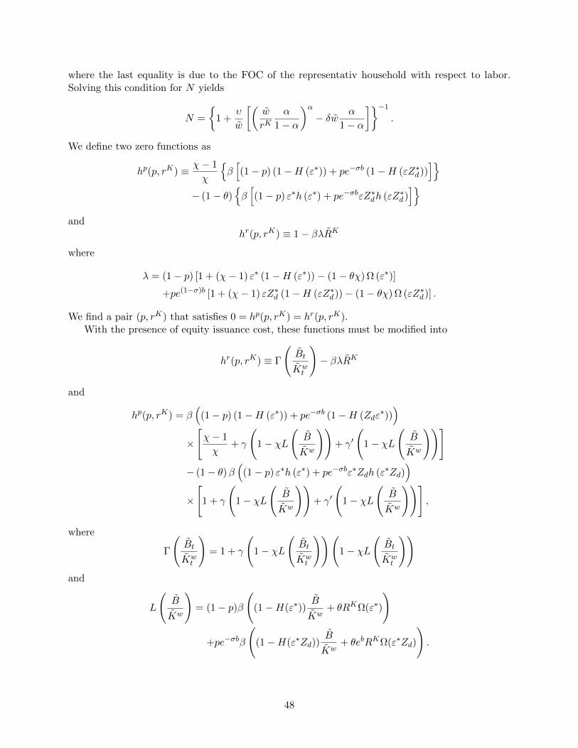
where the last equality is due to the FOC of the representativ household with respect to labor.Solving this condition for N yields
N =
1 +
υ
w
[(w
rKα
1− α
)α− δw α
1− α
]−1
.
We define two zero functions as
hp(p, rK) ≡ χ− 1
χ
β[(1− p) (1−H (ε∗)) + pe−σb (1−H (εZ∗d))
]− (1− θ)
β[(1− p) ε∗h (ε∗) + pe−σbεZ∗dh (εZ∗d)
]and
hr(p, rK) ≡ 1− βλRK
where
λ = (1− p) [1 + (χ− 1) ε∗ (1−H (ε∗))− (1− θχ) Ω (ε∗)]
+pe(1−σ)b [1 + (χ− 1) εZ∗d (1−H (εZ∗d))− (1− θχ) Ω (εZ∗d)] .
We find a pair (p, rK) that satisfies 0 = hp(p, rK) = hr(p, rK).With the presence of equity issuance cost, these functions must be modified into
hr(p, rK) ≡ Γ
(Bt
Kwt
)− βλRK
and
hp(p, rK) = β(
(1− p) (1−H (ε∗)) + pe−σb (1−H (Zdε∗)))
×
[χ− 1
χ+ γ
(1− χL
(B
Kw
))+ γ′
(1− χL
(B
Kw
))]− (1− θ)β
((1− p) ε∗h (ε∗) + pe−σbε∗Zdh (ε∗Zd)
)×
[1 + γ
(1− χL
(B
Kw
))+ γ′
(1− χL
(B
Kw
))],
where
Γ
(Bt
Kwt
)= 1 + γ
(1− χL
(Bt
Kwt
))(1− χL
(Bt
Kwt
))and
L
(B
Kw
)= (1− p)β
((1−H(ε∗))
B
Kw+ θRKΩ(ε∗)
)
+pe−σbβ
((1−H(ε∗Zd))
B
Kw+ θebRKΩ(ε∗Zd)
).
48