! 1!

!The Transmission of Monetary Policy Within Banks:

Evidence from India 1

Abhiman Das IIM Ahmedabad and Reserve Bank of India

Prachi Mishra

IMF and Reserve Bank of India

Nagpurnanand Prabhala CAFRAL and University of Maryland, College Park

November 2015

Between 1996 and 2013, India’s central bank injected or drained liquidity from banks through changes in cash reserve requirements. We analyze the lending responses to these quantitative tools of monetary policy using branch level lending data. We focus on the within-bank variation across different branches of the same bank, controlling for variation between banks stressed in prior work through a saturated specification with interactive bank-year and region-year fixed effects. We show that the intra-variation is important and that branch level asset, liability, and organizational variables explain the intra-variation. Branches that are larger, make loans with smaller ticket size, are deposit-rich, make shorter term loans, have fewer non-performing assets, and with greater managerial capacity respond more to monetary policy. Transmission effects are more sluggish in state-owned banks.

JEL classification: E52, G21

!!!!!!!!!!!!!!!!!!!!!!!!!!!!!!!!!!!!!!!!!!!!!!!!!!!!!!!!1 Abhiman Das can be reached at abhiman@iimahd.ernet.in, Prachi Mishra at prachimishra@rbi.org.in, and Prabhala at prabhala.cafral@rbi.org.in. We thank Viral Acharya, Sumit Agarwal, Charles Calomiris, Anusha Chari, Indranil Sengupta, Peter Montiel, Urjit Patel, Raghuram Rajan, Prasanna Tantri, Saugata Bhattacharya, Bernard Yeung, and seminar participants at the ISB CAF summer conference, NUS Business School, Reserve Bank of India, Society for Economic Research in India, UC San Diego, and UCLA for many useful comments and suggestions. The views expressed are those of the authors and not of the institutions they are affiliated with. We retain responsibility for any remaining errors.

! 2!

I. Introduction

Central banks set monetary policy. How the policy is transmitted through the financial

system has been a question of long-standing interest to both policy makers and academics.

Understanding transmission has become especially important after the 2008 financial crisis.

Doubts and debates about the efficacy of fiscal policy, political debates surrounding its size,

scope, and form, plus inside and outside lags in its implementation, have combined to give

monetary policy a central role in macroeconomic stabilization. Central banks around the

world have responded. In the U.S., there have been successive bouts of quantitative easing

programs to increase loanable funds at banks. Other countries in Europe, Japan, and China

have followed similar policies. How banks respond to monetary policies remains an

important question in the years after the 2008 financial crisis.

We provide new evidence on bank responses to monetary stimulus using a large

dataset of over 128 million loans made between 1996 and 2013 in India. The analysis is of

interest from three viewpoints. First, we focus on transmission within banks. We characterize

the variation in lending responses between different branches of the same banks, using

micro-level branch asset, liability, and organizational data. The within-bank study moves the

literature forward on two dimensions. One, we complement the vast literature on variation

across banks stimulated by Kashyap and Stein (2000). While that literature focuses on external

bank-level frictions such as those in raising capital, we highlight the internal organizational

variables can shape lending responses. Two, the focus on branches lets us control for

unobservables through a suite of saturated fixed effects for year, type of bank, as well as

granular, interactive bank-year and local geography-year fixed effects. We can thus soak up

the capital or liquidity constraints by banks every year, the key determinants suggested by

Kashyap and Stein (2000) and the vast literature it has spawned.

The tool of monetary policy, reserve requirements, is another point of interest.

During our sample period from 1996 to 2013, India’s central bank, the Reserve Bank of

India (RBI) extensively uses reserve requirements as instruments of monetary policy.

Changes in reserve requirements (or “CRR,” the cash reserve ratio) directly alter loanable

funds. Lowering CRR releases funds to banks while increases pulls loanable funds from the

banking system. These changes take immediate effect with essentially zero lags. They are

! 3!

applied formulaically as a fraction of bank deposits with no heed to any individual bank’s

specific circumstances. CRR-like reserve requirements are prevalent in many countries.2

Empirically, our sample has significant variation in the use of reserve requirements in

both directions. Moreover, the tools are used well away from environments with zero

nominal interest rates. This point is worth emphasizing. India has historically maintained

high nominal interest rates to combat inflation. However, reserves required under CRR are

not interest-bearing. Thus, loosening monetary stance through lower CRR gives banks

significant profit opportunities as it lets funds currently not earning interest be redeployed

profitably. Thus, the injections or drainages of loanable funds through CRR changes are

economically meaningful tools of monetary policy.

Finally, the financial system in India is an interesting setting to examine bank

responses to monetary policy. India has an old capital market with uninterrupted operations

since 1875. Nevertheless, banks are important. Bank lending represents about 40% of equity,

bank credit, and bonds outstanding, midway between the 20% in the U.S. and 60% in

Germany (Gambacorta, Yang, and Tsatsaronis, 2014). Banks are also interesting because of

their organizational structures. Nationalization in 1969 created a large state owned bank

network with highly regulated entry, branching, and lending (Burgess and Pande, 2005; Cole,

2009). Private bank entry was opened after India’s 1991 economic liberalization. As a result,

India has large private sector lenders that coexist with the state owned banks. Both state-

owned and private banks operate through extensive branch networks. Our sample comprises

150 banks operating through 126,873 branches that are located in 653 administrative districts

spread over 29 states and 7 union territories. Branches are thus important sources of both

economic and econometric variation.3 We find that that the within-variation is a substantial

component of the overall lending variation, and that several branch characteristics explain

this variation in economically sensible ways.

In our study, the key monetary policy variable is the cash reserve ratio or the CRR.

This is the fraction of domestic deposits that banks must maintain at the RBI in non-interest

bearing form. If a bank fails to maintain the minimum CRR, it must pay the RBI a penal

interest rate. Lowering the CRR increases loanable funds while increasing CRR reduces !!!!!!!!!!!!!!!!!!!!!!!!!!!!!!!!!!!!!!!!!!!!!!!!!!!!!!!!2 See, for instance http://www.centralbanknews.info/p/reserve-ratios.html

3 In comparison, the U.S. market has about 6,800 FDIC insured banks and a network of 94,625 branches as of June 30, 2014. See Bank Branches Decline to Lowest Level Since 2005, The Wall Street Journal, September 29, 2014.

! 4!

resources available for lending. Relaxing CRR has two effects. One effect comes from the

fact that funds currently not earning interest can now be deployed profitably. The second is

on bank size. A cut in the CRR also locks up a lower fraction of incremental deposits in zero

interest balances, thereby increasing the marginal profitability of new funds raised.

The study of reserve requirements as monetary policy tools is interesting from other

viewpoints. Reserve requirements are a feature of many emerging markets, so understanding

their role as monetary instruments is of broader interest in emerging markets. Changes in

reserves also free up financing constraints of banks in a fashion similar to programs that

fund banks making loans (Paravasini, 2008). Such programs relax the external financing

constraints of banks. CRR changes operate by unlocking internal funds of banks. As

monetary tools, reserve requirement changes have the same ends as quantitative tools used

in the advanced economies after the global financial crisis such as TALF, TAF, TARP, SMP,

and LTRO, or other large scale asset purchases program (LSAP). Both tools alter liquid

resources available with banks. In this regard, our sample offers an interesting wrinkle. In the

time period we study, there are both cuts and increases in CRR. Thus, we observe both

expanded access to financing as well as the tapering of easy money.

Credit is the dependent variable. Our data come from the Reserve Bank of India

statistical report BSR-1. We aggregate BSR data into 1.04 million bank-branch-year loan

observations and in later tests. The loans are made by 150 state owned, domestic private, and

foreign private banks operating in India. The dataset has identifiers for bank, amount, and

the originating branch. We adapt the Kashyap and Stein (2000) framework to branch level

data. Credit at the bank, branch, and the year level is the response variable. We explain credit

using the monetary policy variable, CRR, plus controls. Interactions between CRR and

branch characteristics capture the inter-branch variation in responses to monetary policy.

To capture higher order interactions, we include triple interaction effects.

To control for unobserved heterogeneity, we include a range of fixed effects. Time

and bank fixed effects control for economy-wide changes and time invariant heterogeneity at

the bank level, respectively. In the more demanding -- and our preferred – specification, we

include a full suite of bank-year interactive fixed effects. These variables control for factors

at the individual bank level that can potentially vary by year. For instance, these variables

control for the external frictions faced by banks including year-by-year variation in these

frictions. Each branch belongs to one of 653 administrative districts in our sample period.

! 5!

We include district-year fixed effects to filter variation across geographic areas within a given

year. What remains is the variation within a bank across branches.

Following Stein (1997) or Skrastins and Vig (2014), lending depends on the

decision-making hierarchies in banks. Lending proposals originate at the branch. Line staff

screen and conduct credit analysis according to processes set or approved by headquarters.

What happens next depends on the nature of the credit. Some credits can be locally

approved while others move up the bank hierarchy to either the division or national level.

We introduce loan and branch characteristics that capture the nature of the lending process

and that can explain the lending responses to monetary stimulus.

We include several branch level variables in our analysis. One category of variables

represents the type of loan. Loan ticket size drives the delegation of loan authority whether

for approval or review. Small loans are handled at the branch level and larger loans require

zonal, regional, or headquarter level approval. Likewise, long term loans require greater

investment in information gathering and analysis. Branches dealing with these more complex

credits are less likely to respond to monetary stimuli. CREDIT TO DEPOSIT RATIO?

Larger branches are likely to be repositories of greater expertise and organizational

capital in lending. These branches are likely to house more senior managers with greater

lending experience and are likely to have better processing capacity to handle loan flows. The

interactions and communications with headquarters are likely to be more, so lending

frictions are likely lower in large branches.

A characteristic likely to drive lending responses is the availability of local resources

at the branch. Whether deposit rich branches lend more in response to monetary injection at

headquarters is an interesting question. Branches not rich in resources may be ready targets

for any new resources available at headquarters. However, if deposit gathering is costly and

headquarters readily funds deficits, branches may have less incentives to gather deposits. In

this situation, headquarters may allocate more resources to branches that raise more internal

deposits. Thus, lending responses can be greater for branches rich in deposits.

We also analyze differences between rural and urban households. This dimension is

of both economic and practical interest. In India, rural branches are characterized by excess

demand for credit relative to supply. Given the excess credit demand in rural areas, the

supply side responses of banks to injections or withdrawal of loanable funds are more likely

to be reflected in greater credit expansion or contraction in rural branches relative to their

! 6!

urban counterparts. These effects are likely to be more pronounced in state owned banks

that have long histories of operation in rural areas.

We next focus on branch-level non-performing assets of a branch. The risk-taking

channel of monetary transmission has attracted great interest. Loose monetary policy is

often blamed for the 2008 financial crisis as it pushed financial firms to seek higher yields

(Adrian and Shin, 2009; Rajan, 2005; Diamond and Rajan, 2009). On the other hand, poor

loan performance can lead headquarters to penalize branches to contain risk-taking. If so,

headquarters would curb risk-taking by branches. If the disciplining argument is correct, high

NPA branches should lend less when resources are freed through CRR cuts. We also

control for local measures of risk-taking and profitability by computing branch-level interest

rate spreads relative to similar size and industry loans throughout the country. The excess

spread is a control for the marginal investment opportunities of the branch akin to marginal

Q, or for omitted credit risks or a “risk-Q” measures at the branch level.

We show that each of the branch-level asset, liability, and organizational variables

matter. The results make the essential point that besides the external constraints faced by the

bank as a whole, its internal organization and organizational process modulate how lending

responds to monetary stimulus. In particular, we find that a cut in CRR increases lending

more in branches that have less complicated loan structures, have more expertise and are

loaded by less bureaucracy, are sustained by local funds, are located in rural areas, and make

less risky loans.

We conduct several tests to understand the heterogeneity of bank responses. We

study differences between state owned and private banks and find that state owned banks

are more sluggish. We distinguish between loosening and tightening episodes. We find that

while there are some interesting asymmetries, both matter. Finally, our results remain robust

to variations in samples, controls, and econometric methods including lags, differencing, and

running horse races with double interactions of monetary policy variables and other

macroeconomic variables.

The rest of the paper is organized as follows. Section II presents a brief review of the

literature, Section III discusses the data. Section IV describes the econometric specification

and identification strategy, Section V presents the empirical findings and tests for robustness

and heterogeneity. Section VI concludes.

! 7!

II. Related Literature

A. Monetary Transmission

To position our findings relative to received work, we briefly survey some of the

relevant work dealing with monetary transmission through the bank credit channel. As

Bernanke and Gertler (1995) point out, received work on the bank lending channel is

motivated by two facts. First, the direct interest-rate effect of monetary policy on spending is

too weak to explain the observed economic aggregates. Second, monetary policy typically

targets short-term rates.4 However, the responses are seen in the spending on long-lived

assets such as durables. Both findings can be reconciled if one introduces a role for

intermediation. Monetary policy has greater potency in models that incorporate its delivery

through banks. In such models banks are special so economic agents rely on banks for

funding. If, for instance, banks themselves face capital, liquidity, or external financing

constraints, monetary policy effects will reflects banks’ constraints in addition to banks’ roles

in maturity, risk, and liquidity transformation.

The above observation has spawned a vast empirical literature on monetary

transmission through banks. We refer the reader to Peek and Rosengren (2013) for a

relatively thorough survey of this literature. Given its focus on banks, a key part of this

literature is to understand how bank lending responds to monetary shocks. The early work

of Bernanke and Blinder (1992) is cast in a time series setting. It examines aggregate data in a

vector autoregression (VAR) setting. Because VAR results do not offer a clean structural

interpretation (Sims, 1980), the literature turns to other methods to better understand the

relation between bank lending and monetary policy. While the specific experiment designs in

the subsequent work vary, a key thrust has been to move from time series analysis and

macro-aggregates to micro-level analyses. The approach of choice in recent studies has been

differences in difference, or how different institutions or markets supplying credit respond

to monetary stimulus.

An early example of the difference in difference approach is Kashyap, Stein, and

Wilcox (1993). They argue that if fluctuations in bank credit supply simply capture effects of

!!!!!!!!!!!!!!!!!!!!!!!!!!!!!!!!!!!!!!!!!!!!!!!!!!!!!!!!4 An interesting exception is the U.S. Federal Reserve’s maturity extension program, or “operation twist” executed in September 2011 (http://www.federalreserve.gov/newsevents/press/monetary/20110921a.htm). This program targeted the entire term structure rather than short rates by selling short term bonds and simultaneously buying long term bonds in an attempt to flatten yield curves.

! 8!

changes in aggregate demand, commercial paper and bank loans should move similarly in

response to monetary policy. However, they report that monetary policy tightening has

asymmetric effects. It increases commercial paper usage but reduces bank credit, consistent

with supply effects in which banks retract credit in response to monetary tightening and

firms shift to commercial paper as a substitute. Kashyap and Stein (1995, 2000) rely on

differences between different types of banks. They show that financially constrained banks

exhibit greater sensitivity to monetary policy.

Peek and Rosengren (2013) note in their review that the work on how transmission

varies across different types of banks is voluminous and continues to attract new work that

exploit newer settings. For instance, whether banks are part of a larger holding company

(Campello, 2002), participation in securitization markets (Loutskina and Strahan, 2009),

internationalization of banks (Cetorelli and Goldberg, 2012), state-owned versus private

banks (Morck, Yavuz, and Yeung, 2014). The literature also include country level studies

focusing on interesting data or institutional differences between countries (Peek and

Rosengren, 1997; Gambacorta, 2005; Jimenez, Ongena, Peydro, and Saurina, 2012). Our

study focuses on variation within rather than across banks.

B. Internal Capital Markets of Conglomerates

The branch structure of banks resembles the divisional structure of conglomerates,

whose resource allocation decisions and internal capital markets are an important focus of

the corporate finance literature (Maksimovic and Phillips, 2013). The literature asks how

funds are allocated within corporate conglomerates. Our study sheds light on this issue as we

observe resource allocation decisions of individual organizational entities within branch.

Each branch in India is managed by a branch manager who is delegated decision-making

authority with oversight from headquarters.

The branch structure differs from conglomerates in interesting ways. Perhaps the

most pronounced difference is the liability side. In conglomerates, resource raising is at the

headquarters and divisions are allocated capital through internal capital markets (Berger and

Ofek, 1995; Stein, 1997; Maksimovic and Phillips, 2013). However, in banks, branches can

and do raise their own funds through deposits. Any excess is supplied to internal capital

! 9!

markets or deficits sourced from these markets through transfer pricing arrangement.5 With

greater homogeneity in assets, liabilities and human resources, and ongoing supervisory,

operational, and personnel exchanges between branches, the soft information gaps between

branches and headquarters are less pronounced than in conglomerates. The branch structure

is also organizationally different from the bank holding company structure in which each

bank is a legally distinct entity (Avraham, Selvaggi, and Vickery, 2012; Campello, 2012). We

find that these differences lead to interesting variation in how resources are allocated in

response to financing stimulus.

C. Financing Frictions

Understanding financing frictions is key in the corporate finance literature.

Measuring financial constrains is a key focus of the literature. Whited and Wu (2006) and

Ball, Hoberg, and Maksimovic (2015) discuss alternative methods of inferring financing

frictions. A related question is whether financing frictions affect investment decisions of

firms and why. Recent evidence on this evidence include Hennessy and Whited (2007).

Indeed, the existence of such frictions and their potential effects on investment are central in

the analysis of Kashyap and Stein (2000).

Our study informs the financing frictions literature. Changes in reserve requirements

inject funds into banks, relaxing financing frictions, or retract funds from banks, imposing

financing frictions. We study the responses of banks to such stimuli, specifically the internal

allocation of resources to funding shocks. CRR changes release funds or withdraw them at

the corporate headquarters level. The lending responses we observe are the internal resource

allocation outcomes within the organization. Our work is close in spirit to Lamont (1997),

who examines whether cash flow shocks to one division alter the investments in other

divisions of oil companies. We study funding shock at the corporate level and the resulting

resource reallocation across the entire organization.

Relatedly, Campello (2002) argues standalone banks are more sensitive to funding

shocks than banks that belong to a conglomerate holding company. We take this work

further by examining variation inside standalone banks. We show that the allocation of flows

!!!!!!!!!!!!!!!!!!!!!!!!!!!!!!!!!!!!!!!!!!!!!!!!!!!!!!!!5 In India, guidelines for transfer pricing via internal capital markets are provided by the Reserve Bank of India via notification https://www.rbi.org.in/scripts/NotificationUser.aspx?Id=85&Mode=0 .

! 10!

is different. We find that more dependent branches are less sensitive to funding shocks,

consistent with allocation systems that match resource raising by branches. Paravasini (2008)

studies lending when Argentinian banks, particularly small local banks, who receive external

finance through the MYPES on-lending program between 1993 and 1999. The banks receive

$0.75 in financing for every $1 of lending to qualified small firms. Ours is a different

experiment. The relaxation of CRR releases internal funds at headquarters and banks are free

to reallocate the funds as they see fit, as release is not conditional on on-lending

commitments. Thus, the treatment shares feature that it is applied formulaically across all

banks but does not require uptake by the treated.

!III. Data and Descriptive Statistics

A. BSR Dataset

Our data come from the Basic Statistical Returns 1 (BSR 1) collected by the RBI.

Other work using this data includes Cole (2009) and Kumar (2014), who analyze the data at

the bank rather than the branch level. The dataset reports loans outstanding annually by

every branch of every scheduled commercial bank in India. The report comprises two parts,

BSR 1A and BSR 1B. The BSR-1A report compiles all accounts with individual credit limits

above a cutoff, which was INR 25,000 until March 1999 and INR 200,000 after March

1999.6 For credit limits below the cutoffs, amounts are consolidated at branch levels by

broad occupational categories and reported as aggregates by branch.

BSR-1A contains a number of useful fields that we exploit in our analysis. These

fields include location, which refers to the district where credit is utilized. India has a federal

structure in which the nation is divided into states or union territories, each of which is

subdivided into districts. There are currently 36 states or union territories that comprise 630

administrative districts. The data also identifies the credit utilized according to the

population agglomeration group. Rural branches are located in census city centers covering a

population of up to 10,000, semi-urban branches between 10,000 and 100,000, urban

branches between 100,000 and 1 million and metropolitan branches cover areas with

population exceeding 1 million. We create a single category called “urban” by combining the

!!!!!!!!!!!!!!!!!!!!!!!!!!!!!!!!!!!!!!!!!!!!!!!!!!!!!!!!6 For regional rural banks, a category of rural banks sponsored by a larger bank that accounts for less than 4-5% of credit, the cutoff was revised in March 1998.

! 11!

semi-urban, urban, and metropolitan branches. The branch classifications by location do not

vary significantly over time. A relatively small number of the bank-branches, about 5%,

change classifications over our sample period.7

The loan amount outstanding is as of the last reported date. We use it to generate

branch aggregates as well as average loan size. Loans are classified into categories such as

cash credit, lines of credit or term loans. BSR-1A classifies loans into short, medium or

long-term loans of maturity greater than 3 years. The activity and type of organization

indicates the ownership of the borrower, for instance, private owned versus state-owned

borrowers or households. The nature of the borrower account indicates whether the loan is

to small, medium or large enterprises per the prevailing definition at the time of the loan,

whether the loan is to trade or service sectors or the agricultural sector. Agricultural loans are

of particular interest in India. Cole (2009) argues that these loans represent misdirected

credit used for political purposes and tend to increase in consonance with electoral cycles.

We also obtain data on whether an asset is non-performing or not. Indian banks

classify assets as standard, sub-standard, doubtful, or loss assets. We classify assets as either

standard or non-performing assets (NPAs). This figure is computed at the branch level. We

obtain the interest rate on the loan, which we later use to generate measures of excess

spreads at the branch level. While the BSR-1A report gives data on bank assets,

supplementary liability and organizational data come from BSR-2. We extract bank liability

data from BSR-2 to develop branch level measures of the credit-to-deposit ratio and of

banks that lose or gain deposits. BSR-2 also gives us data on branch staffing. We obtain the

number of officers in a branch, which can proxy for the expertise in a branch. We also

obtain the non-officer staff count in a branch. This can proxy for the processing capacity in

a branch or the supervisory demands on branch managers.

We aggregate the loans at the branch level to create a panel dataset in which a unit of

observation is a bank, branch, and year. The branch data are reported as of fiscal year-end,

which is March 31 in India. For example, there are 128 million loan accounts as of March

2013. We sum up the loans by branch to obtain aggregate lending at the bank-branch-year

!!!!!!!!!!!!!!!!!!!!!!!!!!!!!!!!!!!!!!!!!!!!!!!!!!!!!!!!7 As a robustness check, we also broaden the definition of “rural” to include “semi-urban” areas and find similar results. The main findings in the paper are robust if we exclude the small number of the bank-branches whose classification changes during our sample period.

! 12!

level and where relevant, at a more granular level. The dataset provided to us begins in the

fiscal year ending March 31, 1996 and ends on March 31, 2013.

B. Branch Networks

Table 1 provides a snapshot of the bank lending data at the end of fiscal 2013. The

data cover 150 banks. There are 26 state owned (public sector) banks, 20 domestic private

banks, 40 foreign-owned banks, and 64 regional rural banks (RRBs). Figure 1 shows how the

number of banks has changed over time. The number of state owned banks has remained

roughly the same. The number of private sector banks decreases to about 20 at the end of

our sample period. The number of foreign banks has increased from 28 to 40 after the global

financial crisis but they tend to maintain small operations.

Branch networks have been a major thrust of the banking regulations in India,

particularly after India’s bank nationalization program in 1969. Branches have historically

been seen as distributive instruments that foster economic development. The branching

regulations incentivized expansion of rural branch networks in India between 1969 and 1990

so bank branches served currently underserved areas (Burgess and Pande, 2005). As

attention shifted towards credit needs more broadly and the financial soundness of the

banking system, policies required banks to pay due attention to the commercial viability of

branches, roughly concurrent with the 1991 “big bang” economic and financial liberalization

in India. Our sample begins about 5 years after these changes and has a relatively stable bank

branching regulatory structure.

To place the branch level analysis in context, it is useful to point out that bank

branching is also an important regulatory focus in the US. The structure is, however,

somewhat different as interstate banking compacts and laws govern how banks may expand.

Jayaratne and Strahan (1996) and Karthik, Nandy, and Puri (2015) study these variations to

examine the nexus between bank financing and growth. In India, banking regulations are

national rather than at state level. Thus, banks have been relatively free to move across state

borders and India has had relatively few banks with national franchises. The largest bank in

India, the State Bank of India, has 20,833 branches compared to Wells Fargo, whose roughly

6,300 branches endow it with the largest branch network among the U.S. banks.

The banks in our sample have 126,873 branches. Figure 2 displays the time trends in

branch networks. The number of rural branches is relatively stable in the early years of our

! 13!

sample but starts increasing after 2006. The number of rural branches increases by roughly a

quarter over the entire sample period. Urban branching witnesses a steady and intensifying

growth over the sample period. The number of urban branches more than doubles during

the sample period. The share of rural branches has decreased from 43% to 30% over the

sample period.

C. Lending

In keeping with local practice, we express lending in local currency. The monetary

unit of analysis in India is typically one thousand crore Indian rupees (INR) where 1 crore =

10 million rupees. The exchange rate in June 2015 is roughly about US$1= INR 65, so $1

million ≈ INR 65 million. Table 1a shows that the average lending by a banking institution is

about INR 37,000 crores (about $ 5 billion). There is significant variation in this figure by

bank type. On average, state owned banks lend Rs. 157,000 crores ($24 billion), roughly

three times the average lending by a private bank (Rs. 52,500 crores).

State owned banks account for about three-quarters of the total lending. Private

banks have the second largest market share at about 20%. Regional rural banks (RRBs) are

entities that are sponsored by and operate under the umbrella of other banks. They cater to

rural areas and represent a means of using the infrastructure of existing banks to reach

underserved rural areas. Although there are several RRBs, they comprise a very small

fraction of the market share (2%). On average, they lend far less than public or private

banks. For instance, the average lending by an RRB is about Rs. 2,000 crore ($300 million),

which is less than 5% of the amount loaned by a public sector bank. Regional rural banks

(RRBs) maintain a small 2.5%-3% share in the sample period. Given their relatively small

size, we exclude RRBs from our analysis. Our main results are robust to including the RRBs.

Table 1b and Figure 3 describe how banks and branches expand over time. Table 1b

shows that in India, the number of banking institutions actually shrink over time from 283 in

1996 to 150 in 2013. At the same time, the number of branches increase from 62,465

branches in 1996 to 101,603 branches today. The average credit per branch increases from

roughly INR 4 crores (USD 0.6 million today) to INR 54 crores (USD 8 million), a 13-fold

increase in a time period when GDP grows 7 times and the number of branches increase

1.62 times. Thus credit per branch expands more than the economy and comes at the same

time as the number of banks actually shrinks.

! 14!

Table 1c provides further evidence on the economic importance of branches

through a two-way decomposition of variance. The variation within banks is small relative to

variation across branches. The within-bank across branches variation accounts for 90% of

the variance in lending compared to 73% in 1996. The within-district variation across banks

similarly shrinks. It accounts for 14% of the variation between banks in 1996 versus 9%

today. Within bank or branch variation inside districts accounts for 86% of the variance in

1996 and 91% in 2013. Branches have been historically important and their importance has

increased today. Informal conversations with private an public sector bankers confirm this

point. Branches are increasingly delegated authority for lending decisions for which expertise

likely resides in branches. In one bank we talked to in 2015, a typical branch manager can

automatically sign off on loans of up to INR 20 million, or about $300,000. Relatively few

businesses are handled through centralized verticals. The necessary credit infrastructure and

information production services are still developing.

Figure 3 shows how the market shares of different types of banks evolve over time.

We divide state owned banks into the State Bank of India (SBI) group and the rest. SBI is

the largest state owned bank in India. Its market share declines from 29% to 23% between

1996 and 2013. The remaining state owned banks have about a 50% market share in

aggregate credit in our sample. Private banks grow significantly in our sample period. Their

share in total lending increases from 8% to 19% between 1996 and 2013. Foreign banks

have a relatively small presence and their market share declines over our sample period from

9% to 5%. Many foreign banks maintain small branch networks and geographical footprints.

Figures 4-6 display data on lending by branches. Figure 4 shows that urban branches

comprise the large fraction of bank lending, accounting for about three quarters of all

lending. This is a striking mirror image of the 27% of the Indian population living in urban

areas according to the 2001 Indian census. Figure 5 displays the number of accounts in our

sample. The number of loan accounts increases in both urban and rural regions especially in

the later part of our sample period. In 2013, urban branches had close to 80 million loan

accounts, which account for close to 70% of all accounts in our sample. Figure 6 displays the

average loan ticket size. We find that the ticket size increases over the period and the

increase is especially pronounced outside the urban areas. For instance, the average ticket

size of the loans made by rural branches in 1996 is Rs 13,000, or about $200 at an exchange

rate of US$1 = INR 65. It increases almost 10-fold Rs. 126,000 (≈ US$ 2,000) in 2013. In

! 15!

urban branches, the increase in ticket size over the same period is about 7X, from Rs. 87,000

($1,300) to Rs. 638,000 (about $9,900).

We compute bank concentration at the district level using two measures. One is C4

or the share of lending by top 4 banks. The other is the Herfindahl index (HHI), which is

the sum of square of the market shares of banks. According to the U.S. Department of

Justice, a value of the index above 2500 indicates highly concentrated markets.8 By either

metric, C4 or the Herfindahl index, Figure 7 shows that the average bank concentration has

been high and continues to remains high. Concentration ratios vary by location. Figure 8

shows that urban areas exhibit higher branch saturation and greater levels of competition

while rural areas are more concentrated.

D. Reserve Requirements and Monetary Policy Tools

The CRR is the fraction of bank deposits that banks must keep with the RBI in the

form of a noninterest bearing deposit. Cash reserve requirements of this sort are used in

several other countries although their size, nature, and main purpose vary across the world.

The reasons for holding reserves include a prudential motive to limit bank risk-taking and

prevent panics, monetary control, and liquidity management (Gray, 2011). The UK has no

reserve requirements. U.S. banks must keep reserves in accordance with the Federal Reserve

Regulation D over the reserve maintenance period of 14 days beginning Thursdays and

ending Wednesdays.9 The Chinese central bank has altered reserve requirements close to a

dozen times after the 2008 financial crisis. We obtain the data on reserve requirements, the

key monetary policy instrument we study, from publicly available data distributed via the

Reserve Bank of India website.

Related to the CRR is the statutory liquidity ratio (SLR), which represents the fraction

of demand and time deposits that banks operating in India must hold in approved assets.

Bonds issued by the Indian central government or the state governments constitute the bulk

of banks’ SLR holdings although smaller portions of deposits also flow to other SLR-eligible

assets such as cash and gold. Figure 9 shows the evolution of CRR and SLR. The CRR

exhibits more frequent variation over time, moving from 14% to 4% with an intermediate

!!!!!!!!!!!!!!!!!!!!!!!!!!!!!!!!!!!!!!!!!!!!!!!!!!!!!!!!8 See U.S. Department of Justice and the Federal Trade Commission Horizontal Merger Guidelines (2010).

9 See http://www.federalreserve.gov/monetarypolicy/files/reserve-maintenance-manual.pdf

! 16!

trough and peak of 4% and 8%, respectively. These figures are proportions of aggregate

bank deposits so the changes are economically meaningful. The SLR has decreased from

31.5% to 22% of deposits, with much of the reduction driven by a change in 1997. Adding

the CRR and SLR gives an indication of the quantity of investible resources available for

banks. Investible funds are about 74% of bank deposits in 2013 versus 54.5% in 1996,

indicative of the increased liberalization of the banking environment in India.

Is SLR a monetary policy tool? Perhaps, from two viewpoints. One, changes in SLR

are announced in the monetary policy statements. Additionally, SLR changes allow banks to

reallocate funds from risk-free assets to loans. On the other hand, SLR may be viewed as a

constraint on portfolio allocation of banks. Because SLR holdings are usually interest-

earning securities, the lending responses to SLR changes are likely to be attenuated relative

to CRR responses, which alter the quantities of non-interest earning assets. Empirically,

there are few changes in SLR during our sample period. Discussions with policy-makers

suggest that the CRR rather than SLR as monetary instruments. We thus focus on CRR

alone but also consider specifications with both CRR and SLR. Empirically, there are few

changes in SLR during our sample period. We thus focus on CRR alone but also consider

specifications with both CRR and SLR.

While our focus is on the CRR as a quantitative instruments of monetary policy, we

also control for policy rates. We include the RBI’s repo rate in our econometric models. The

RBI conducts daily monetary operations through a Liquidity Adjustment facility that lets

banks borrow or lend money through repurchase (repo) or reverse repurchase (reverse repo)

agreements, respectively. The monetary operations are conducted to achieve repo rates

targeted by the RBI. Since 2011, the reverse repo rate is set at a fixed band of 100 to 300

basis points below the repo rate. Figure 10 graphs the evolution of repo and reverse repo

rates since 2001. Both rates are highly correlated and move in the same direction. In the

empirical analysis, we focus on the repo rate as a control.10

Figure 11 shows that the policy rate and quantity instruments have often moved in

the opposite direction. For example, between 2011 and 2012, while monetary policy was

tightened based on interest rate instruments, it was loosened through quantity instruments.

!!!!!!!!!!!!!!!!!!!!!!!!!!!!!!!!!!!!!!!!!!!!!!!!!!!!!!!!10 The results in this paper are robust to using a composite price instrument, defined as an average of repo and reverse repo rates.

! 17!

A wbody of the monetary policy literature uses other measures of monetary stance such as

the narrative approach used by Romer and Romer (2004) or semi-structural VAR methods

used in Bernanke and Mihov (1997). These measures are less developed for the Indian

market so we do not consider them in our analysis.

!IV. Empirical Strategy

Our focus is on the heterogeneity in lending response across branches within the

same bank. However, following Kashyap and Stein (2000) and the related work on bank

transmission, it is necessary to control for variation across banks. We do so by including

bank effects and bank-year interactive effects. For instance, it!controls for time-varying

demand side factors including those that vary differentially across banks. As importantly, it

also controls for idiosyncratic bank-specific factors such as its CEO changes or balance

sheet conditions that vary from year to year and from bank to bank.

Likewise, we include granular fixed effects at the level of the administrative district

times the year, which controls for local geography as well as idiosyncratic events within a

geography such as a shortfall in rain in a particular year.

Our baseline regression is:

lnLijt =α +βBijt−1 +δMtBijt−1 + s iπ t + sdπ t +εijt (1) ,!

where Lijt is the value of lending by bank i at branch j in year t. Bijt−1 stands for a suite of

variables at the branch level that we discuss later and is observed at t-1. Mt is the quantitative

policy tool, usually the average CRR in year t. The variables si !and π t denote bank and year

fixed effects respectively while the variable s iπ t !represents the interactive bank-year fixed

effects. Likewise, variable sd denotes district fixed effects and sdπ t denotes interactive

district-year fixed effects. Standard errors are clustered at bank-branch level but clustering at

bank level produces similar results. The overall approach is like Kashyap and Stein (2000)

approach or its recent variants such as Jimenez, Ongena, and Saurina (2012).

In Eq. (1), the coefficients δ are the main objects of interest. They capture how the

effect of monetary policy depends on branch characteristics. We include variants of

specification (1) for further insights into monetary transmission. We also consider models

with triple interactions, for instance models that have state owned and private sector banks.

! 18!

Following Jimenez, Ongena, and Saurina (2012), we also run a horse race in which

interactions with the monetary variables Mt compete with interactions with other annual

macroeconomic variables such as inflation, or other monetary tools.

!V. Main Results

As discussed earlier in Sections II and III, bank branches are important sources of

economic variation in lending. We examine the branch-level variables that help explain this

source of variation. The key variables of interest are branch level variables, specifically the

coefficients for the interaction of branch characteristics and monetary policy, i.e., δ in

equation (1). We classify a branch as high on a particular dimension if its characteristic

exceeds the median level for all branches. A negative sign for the interaction term indicates

greater responsiveness to monetary stimulus while a positive sign indicates a slow response.

For efficiency and compactness, this section both motivates the variables and

discuss the relevant results. We discuss the direction of results in terms of a stimulus that

relaxes the CRR, or loosens the monetary policy but the discussion is easily recast in

tightening terms as well. Table 2 reports the coefficients when the variables are included one

at a time. Table 3 reports the results in a multivariate setting. Most results are similar across

the tables so we focus on the full multivariate specification estimates in Table 3. We also

include the caution that the number of observations vary across the specifications. This is

because some variables of economic interest are compiled in the RBI’s BSR returns only

after 2008. For specifications with these variables, the number of observations is lower but is

reported in the tables.

A. Loan Size and Maturity

The first set of variables are based on the loan type. The central idea is that

transmission is likely to be weaker for loans that place greater demands on bank

organizational hierarchies. Loan size is perhaps the first proxy for lending decisions that

must be pushed up bank hierarchies. Delegation of authority to branches is often based on

loan size. For instance, in a large nationalized bank in India, loans of up to INR 20 million

(about US$300,000) can be sanctioned by the branch manager directly but larger loans must

go up the for credit approval. Longer term loans are similarly more complex. Making a case

! 19!

for a longer term loan is more burdensome than for a short-term line of credit secured by

current assets. Moreover, long-term loans are not easily reversed. Models of reversible

investments predict that commitments are less likely to be made, or agents will “wait to

invest” when decisions are not easily reversed (McDonald and Siegel, 1986; Pindyck, 1988;

Veracierto, 2002). In Table 2, the ticket size interaction with monetary policy is not

significant but it becomes significant in the full multivariate specification in Table 3. The

interaction term for branches with greater share of long-term loans is positive and significant

in both tables. Thus, branches making more high ticket size loans or long-term loans are

more sluggish to respond to monetary stimulus.

B. Credit to Deposit Ratio

A branch’s credit to deposit ratio indicates the extent to which a marginal dollar of

deposit raised is deployed within the geography served by the branch. In an environment

where deploying credit is costly, it is easy to show that credit to deposit ratios are negatively

correlated with the marginal costs of deploying one dollar of incremental credit. For

instance, branches with diffuse customers spread over difficult terrain may find it more

costly to acquire new lending customers and due enough due diligence to evaluate customers

and make loans. A dollar of loanable resources is more likely to flow to central transfer

pricing pools at lower spreads instead of spending resources to find and evaluate new credit.

Thus, when monetary policy loosens, we expect branches with higher credit to deposit ratio

to exhibit a greater response than branches with low credit to deposit ratios. Table 2 reports

results consistent with this view. In Tables 2 and 3, the interaction coefficient for credit to

deposit ratio is negative and significant, suggesting that branches with high credit to deposit

ratios respond more to CRR changes.

C. Branch Size

The core hypothesis here is related to branch level expertise in originating and

processing loans. Extending credit requires expenditure in customer acquisition, judgment

about credit quality, expertise in assessing credit needs and finding suitable credit products to

fit the needs, helping borrowers put together the necessary loan application package, and

managing the application process. Greater loan volumes give branches the experiential

knowledge to better handle lending pressures. Thus, banks with greater size may find it

! 20!

easier to respond to monetary stimulus. We measure size in two ways. One measures the

total branch assets relative to assets of other branches within the same bank. The other

measures branch assets relative to assets of all branches in the banking system. We expect

transmission effects to be greater in large branches using either measure. Both measures of

branch size have negative and significant interaction coefficients. Thus, larger branches tend

to respond more to CRR changes than smaller branches.

D. Branch Human Capital

As discussed above, lending involves several steps ranging from origination to credit

assessment to delivery. Human capital is necessary to handle many of these steps, particularly

in the context of an emerging market like India where credit decision infrastructure is human

capital intensive even today. To the extent these tasks are not routinized, line officers of the

bank drive lending processes. We obtain measures of the human capital of the branch from

report BSR-2. One measure is the number of officers in a branch and the other is the ratio

of offers to staff in a branch. The officers in a banking system represent high-skill human

capital, particularly in India where bank officer jobs are sought after and involve a very

competitive screening process both in private and public banks.

We also obtain data on the number of clerical staff per officer. This variable can

reflect the branch capacity to conduct the branch’s administration process. Alternatively, it

can also reflect the degree of automation, or more specifically, the lack of automation in a

branch. It can also administrative load on officers, as a low officer-to-clerk ratio places more

demand on the officer’s time to administration as opposed to the lending business of the

bank. We expect that the lending response to monetary stimulus is greater when a branch

has more officers or has a low officer to clerical staff ratio.

The human capital variables are both significant with the predicted sign. Branches

with a high number of officers have a negative interaction term, so these branches are more

responsive to monetary stimulus. Branches with greater clerical staff to officer ratios have a

positive interactive coefficient, so these branches transmit monetary policy less.

E. Local Funding

We examine the extent to which a branch is deposit rich or deposit poor. Our proxy

for this is branch level log deposits. Low deposit branches may be the first recipients of extra

! 21!

funding surpluses at headquarters if the low deposit base reflects less deposit raising

potential in branches. Thus, transmission may be greater for deposit-starved branches.

On the other hand, incentive theories generate the opposite prediction. Deposit

raising is a core activity for banks and involves costly effort. Many banks explicitly set

deposit raising targets for their branches. A headquarters that perennially funds branch

deposit deficits ends up subsidizing branches who make less effort in resource raising. Ex-

post, headquarters will tend to bail out branches if headquarters has preference for large

bank size (Rajan, Servaes, and Zingales, 2000). To countervail such effects, headquarters may

dispense less funds to branches that are poor in deposits, By providing banks matching

resources when they raise their own deposits, the agency problems of slack in deposit raising

are mitigated. The empirical prediction is that transmission is weaker for branches with less

deposits.

Tables 2 and 3 reports the results. The variable of interest is “low deposit,” which

represents branches with deposit levels below the median across all branches of the same

bank in the same year. We find that the interaction term for low deposit levels deposits is

positive. Thus, branches with low deposits transmit monetary policy less. The results are

consistent with the incentive theory viewpoint in which lending resources are channeled

more to branches that raise their own deposits. Headquarters appears to reward branches for

deposit raising activities by matching resources raised by branches.

E. Rural Branches

We next examine whether the bank branch is located in a rural or urban location.

The issue on hand is whether transmission should be stronger or weaker to rural branches

when surplus funds become available at headquarters. There are two possibilities. One is that

the transaction costs of making new loans is higher in rural areas. The distance in lending

between branches and borrowers is likely greater in rural areas (Petersen and Rajan, 2002). In

addition, gathering the relevant soft information necessary for lending may be more difficult

in rural areas. Expansions in rural credit may be driven more by political pressures (Cole,

2009), making rural credit less elastic to monetary stimulus.

! 22!

The opposite prediction, or greater transmission in rural areas, comes from the

viewpoint that rural areas are characterized by perennial credit shortages.11 For instance,

credit to deposit ratios of rural branches are about 14-20% lower than ratios for urban areas.

Credit constraints of rural customers have been the primary motive for nationalization of the

banking industry, and subsequent branch expansion and licensing norms. They have also

resulted in birth of microfinance industry. Thus, in a monetary expansion, the excess

demand makes it easier for banks to push out credit to rural areas. Likewise, during

contractions, pulling back credit is always possible but the threat of lost relationships looms.

But this loss of business is less relevant in rural areas given the plentiful opportunities to

expand given credit deficits so rural credit may be more elastic to supply of funds. We find

support for this latter view in Table 3. Rural branches have negative interaction terms,

suggesting that they transmit monetary stimulus more than their urban counterparts.

G. Non-Performing Assets

We next focus on the level of non-performing assets of a branch. The link between

loose monetary policy and risk-taking is a familiar theme. Loose monetary policy is often

blamed for the 2008 financial crisis as it pushed financial firms to seek higher yields (Adrian

and Shin, 2009; Rajan, 2005). Perceptions that central banks will ease monetary stance if

there is a crisis may fuel ex-ante risk-taking (Diamond and Rajan, 2009). Jimenez et al. (2012)

find evidence for a risk-taking channel of monetary policy. On the other hand, poor loan

performance at a branch can lead headquarters to penalize branches. If so, headquarters will

push out extra funds released by CRR cuts to branches with low NPAs. We test this

hypothesis by examining the fraction of non-performing assets (NPAs) in a branch. If the

disciplining argument is correct, high NPA branches should lend less when CRR is cut.

We find support for the disciplinary viewpoint of branch monetary transmission.

Branches with greater share of non-performing assets transmit CRR decreases less. Thus

!!!!!!!!!!!!!!!!!!!!!!!!!!!!!!!!!!!!!!!!!!!!!!!!!!!!!!!!11 Karlan and Murdoch (2009), for example, note that “the simplest evidence of a credit market failure comes from evaluation of interventions which show increased use of credit after some shift in supply. This has been shown both for microenterprises (Banerjee and Duflo, 2009 in India; Karlan and Zinman, 2009a in the Philippines), consumers (Karlan and Zinman, 2009b in South Africa) and small and medium enterprises (Banerjee and Duflo, 2008 in India). Had these studies showed instead a substitution from one source of credit (presumably more expensive on some margin) to another, the evidence of credit constraints per se would not have been as clear.”

! 23!

headquarters appears to curb risk-taking by branches. The results are a striking contrast to the

viewpoint that banks engage in excessive risk-taking when monetary policy is loosened.

H. Interest Rate Spreads

We compute a branch level interest rate spread variable as follows. Using the BSR-1

interest rate data, we compute the size decile-bucket and sector-specific interest rates in each

fiscal year. We then compute the spread of each loan as the excess of the loan interest rate

over its size and sector matched average for the year. The weighted average of the excess

spread for each branch represents the excess spread charged by a branch.

The excess spread can be interpreted in two ways. One is that it is a control for the

marginal investment opportunities of the branch, similar to a branch-level Q in a theory of

Q-investment. This is because the excess spread measure is risk-adjusted and thus reflects

the profits that the bank generates relative to its peers lending in the same sector and making

similar sized loans. From this viewpoint, banks with greater excess spreads should have

greater lending responses when CRR is reduced. Excess spread could also be a control for

omitted credit risks that the branch sees but the econometrician does not. From either

viewpoint, the more important point is that the excess spread is likely to be a useful variable

as a catch-all control omitted risks or omitted lending opportunities. We thus include it in

the regression specifications.

In Table 2, we find the coefficient is positive but not statistically significant. In the

multivariate specification in Table 3, the coefficient for spreads is positive and significant.

Branches with greater loan spreads have lower lending responses to CRR cuts. The result is

more consistent with the view that loan spreads reflect unobserved credit risk rather than

marginal Q of branches, which are probably picked up through the suite of district-year fixed

effects in our specification.

I. Year Fixed Effects Replaced by CRR

Table 4 presents a version of the multivariate specification in which the year fixed

effects are replaced by the reserve requirements in the year. This specification clearly places a

structure on the annual fixed effects by replacing them by the annual CRR and is thus less

general than including the appropriate year fixed effect that can capture a whole slew of

macroeconomic conditions. However, with the caveat, the specification has some value, as it

! 24!

lets us to see the net effect of monetary policy, which is the coefficient for the CRR in Table

4. We find that the coefficient for CRR is negative, so the overall effect of CRR reductions is

to increase lending. The signs of the branch variables remain unchanged. The results are

reported for the 2008-2013 period when the full set of explanatory variables are available.

J. State Owned Banks

Table 5 focuses on lending responses by banks with different ownership structures.

An interesting characteristic in the emerging market context is the state ownership of banks.

Morck, Yavuz, and Yeung (2014) find that monetary policy is more significantly related to

credit in countries a larger fraction of the banking system is state controlled. They explain

these findings with the hypothesis that managers in state-owned banks are likely to be more

responsive to political pressure, and thus more cooperative with monetary policy. Deng,

Morck, Wu, and Yeung (2013) analyze the case of China. They show that the effectiveness

of the 2008 monetary stimulus in China is linked to state-controlled banks’ managers’

obedience to the Communist Party hierarchy, rather than to the effectiveness of standard

transmission channels.

In India, the government does not have the same degree of leverage over banks.

Managerial appointments and operating decisions at the lower level are largely free from day

to day interference from the government. However, the government does enjoy soft and

hard influence at the strategic level through the upper hierarchy of banks, for instance

through its ability to appoint top management and board members (Cole, 2009). Moreover,

government owned entities, state owned banks operate by an encumbering set of rules and

regulations that make them speedy responses difficult. From this viewpoint, state owned

banks may be slower to respond to monetary policy.

Table 5 reports the results for state owned and private banks separately. The

contrasting view is that state owned banks may transmit policy less. The results in Table 5

are broadly consistent with the slower-transmission viewpoint of state owned banks.

Coefficients are generally lower for state owned banks relative to private banks. In one case,

non-performing assets, the coefficient becomes insignificant. Private banks are more

conscious of pushing loans to branches that have poor performance records. The rural

branch coefficient flips signs for private banks. Thus, rural branches of private banks are less

! 25!

elastic to CRR changes. Rural branches of state owned banks are more likely to respond to

CRR changes and drive the aggregates reported in Tables 2 and 3.

K. Loosening and Tightening Episodes

Table 6 analyzes the results for loosening and tightening episodes. Loosening

episodes are defined as those in which CRR changes are negative, or banks have lower CRR

requirements or more free resources to lend. A negative coefficient, with a larger magnitude,

indicates a greater lending response. We find that during loosening episodes lending

increases more in response to a CRR change, for branches with low ticket size, short-term

loans, high credit-to-deposit ratio, more officers, greater deposits, and rural branches.

Surprisingly, the coefficient for non-performing assets flips signs relative to Tables 2 and 3,

even during loosening episodes, suggesting that risk-taking increases in loosening episodes.

When CRR increases, banks have fewer resources to lend, so the specification

estimates pick up the areas where lending tightens. A negative coefficient indicates more

retraction of lending. We find that branches with high ticket size, long-term loans, high

credit to deposit ratio, low deposits, high interest rate spreads, and high NPAs cut back

more. The coefficient for rural is insignificant, suggesting low elasticity of rural credit to

CRR changes.

L. Other Robustness Tests

In the next robustness tests, we exclude a large state owned bank, the State Bank of

India (SBI) and its affiliates. The SBI group accounts for about a quarter of the total bank

lending on average over the sample period. Table A1 shows that the group has an extensive

network with over 20,833 branches. Given its size, it is an especially attractive target for

government influence and is more likely to act in line with government priorities. Excluding

SBI and its affiliates does not alter the main results. We next include regional rural banks

(RRBs) in the sample. In the baseline regressions, RRBs are excluded as their share in overall

lending in less than 3% and has remained stagnant over time. Including many RRBs in a

branch level regression could overstate the results relative to their economic importance. .

Table 7 reports the results. The most significant change is in the coefficient for rural

branches, which becomes insignificant when we drop State Bank of India, reflecting the

bank’s muscle in rural areas from its long operating history in India. The inclusion of

! 26!

regional rural banks mutes the significance of the rural branch coefficient. Other branch

asset, liability, and organizational variables remain similar.

Table 8 address two other issues. One is that the differential response of bank

lending within branches could also be driven by macroeconomic variables other than

monetary policy. Following Jiménez, Ongena, and Saurina (2014), we include the interaction

between a key macroeconomic variable, the inflation rate, with the monetary policy variable.

This is a horse race where interactions of the rural branch dummy variable with the

monetary policy are stacked against similar interactions with inflation. Cole (2009) points out

that electoral cycles can drive variation in lending. Cole finds an election cycle component of

lending driven by the timing of state-level elections, particularly in sectors vulnerable to

political capture. To control for potential confounding effects from elections, we include

relevant dummy variables for state elections as controls. We include dummy variables for

election years and their interaction with the rural branch dummy. Our results remain similar

and robust to these variations in specification.

Our focus is the changes in cash reserve ratio. In Table 9, we examine the robustness

of the specification to two other variables. One is the policy rate, which is the RBI’s repo

rate available to banks through the repo window. The other is the statutory liquidity ratio,

SLR, which is the fraction of reserves required to be held in government securities, which is

subject to occasional changes but concentrated towards the start of our sample period.

Finally, the last tests examine alternative econometric specifications. We lag the

monetary policy variable by one year to address feedback issues related to using

contemporary monetary policy. We also report the results with the specification in

differences. The dependent variable is the difference in lending. Finally, we also include a

lagged dependent variable in the model. Models with a lagged dependent variable and fixed

effects can pose problems as the estimates are not consistent. However, simulation evidence

in Buddelmeyer, Jensen, Oguzoglu, and Webster (2008) suggest that the bias reduces when

there are a large number of cross sectional units, as is the case in our study. While these are

not standard models employed in the vast literature on the bank lending channel literature

we nevertheless estimate these models as robustness. The results are not qualitatively

different.

! 27!

VI. Conclusions

A very old and basic question that has attracted the attention of both academics and

policy makers around the world is: how does monetary policy work? Despite the existing

vast literature on the topic that primarily spans advanced economies, the effectiveness of

monetary policy remains an extremely complex issue with many moving parts. This paper

focuses on how monetary policy affects lending by banks using a new and a very large

dataset from India. Our particular focus is on reserve requirements as quantitative tools of

monetary policy that are deployed away from the zero bound in our sample period, on

branch-level responses, or responses within a bank across its different branches, and on

models with saturated bank-year and district-year fixed effects. We find compelling evidence

of cross sectional differences within banks in their responses to monetary policy. The

differences are explained by several branch level asset, liability, and organizational variables,

indicating that the internal organization impacts how banks respond to monetary policy.

VII. References Avraham, Dafna., Patricia Selvaggi, and James Vickery, 2012, “A Structural View of

Bank Holding Companies,” FRBNY Economic Policy Review, 65-81. Ball, Christopher, G. Hoberg, and V. Maksimovic, 2015, “Redefining Financial

Constraints: A Text-Based Analysis,” Review of Financial Studies 28, 1312-1352. Bernanke, Ben S. and Alan S. Blinder (1992), “The Federal Funds Rate and the Channels of Monetary Transmission,” American Economic Review 82(4), pp. 901-921.

Bernanke, B. S., and M. Gertler. 1995. “Inside the Black Box: The Credit Channel of Monetary Policy Transmission.” Journal of Economic Perspectives,9(4): 27–48.

Bernanke, Ben S. and Ilian Mihov (1998), “Measuring Monetary Policy,” The Quarterly Journal of Economics, Vol. 113, No. 3 (Aug., 1998), pp. 869-902.

Berger, A.N., A. Demirguc-Kunt, R. Levine, and J.G. Haubrich (2004), “Bank

Concentration and Competition: An Evolution in the Making”, Journal of Money, Credit and Banking, Vol. 36, No. 3, pp. 433-451.

Bertrand, Marianne and Sendhil Mullainathan. 2003. Enjoying the Quiet Life?

Corporate Governance and Managerial Preferences. Journal of Political Economy 111(5) 1043-1075.

! 28!

Buddelmeyer, Hielke, Paul H. Jensen, Umut Oguzoglu, and Elizabeth Webster

(2008), “Fixed Effects Bias in Panel Data Estimators”, IZA Discussion Paper No. 3487. Burgess, Robin, and Rohini Pande. 2005. "Do Rural Banks Matter? Evidence from

the Indian Social Banking Experiment." American Economic Review, 95(3): 780-795. Campello, M., 2002, Internal Capital Markets in Financial Conglomerates: Evidence

from Small Bank Responses to Monetary Policy, Journal of Finance 57 (6), 2773-2805. Cecchetti, Stephen G.,1999, “Legal Structure, Financial Structure, and the Monetary

Transmission Mechanism,” FRBNY Economic Policy Review (July), pp. 9-28. Cetorelli, N., and L. Goldberg, 2012, “Bank Globalization and Monetary

Transmission,” Journal of Finance 67 (5), 1811-1843. Christiano, Lawrence J. , Martin Eichenbaum, and Charles l. Evans (1996),

“Identification and the Effects of Monetary Policy Shocks,” in M. Blejer, Z. Eckstein, Z. Hercowitz, and L. Leiderman, eds., Financial Factors in Economic Stabilization and Growth (Cambridge: Cambridge University Press), pp. 36-74. Cole, Shawn. 2009. "Fixing Market Failures or Fixing Elections? Agricultural Credit in India." American Economic Journal: Applied Economics, 1 (1), 219-250. Deng, Yongheng, Randall Morck, Jing Wu & Bernard Yeung. 2011. Monetary and Fiscal Stimuli, Ownership Structure and China’s Housing Market. National Bureau of Economic Research Working Paper 16871. Drechsler, Itamar, Savov, Alexi and Schnabl, Philipp, 2015, The Deposits Channel of Monetary Policy. Available at SSRN: http://ssrn.com/abstract=2536230 or http://dx.doi.org/10.2139/ssrn.2536230.

Friedman, Milton and Anna Schwartz (1963, A Monetary History of the United States,

1867-1960 (Princeton: Princeton University Press). Gambacorta, L., Jing Yang, and Kostas Tsatsaronis, 2014. "Financial structure and

growth," BIS Quarterly Review, Bank for International Settlements, March.

Gordon, David B. and Eric Leeper (1994), “The Dynamic Impacts of Monetary Policy: An Exercise in Tentative Identification,” Journal of Political Economy vol. 102, No. 6 (December), pp. 1228-1247.

Gray, Simon, 2011, “Central Bank Balances and Reserve Requirements,” IMF

Working Paper 11-36. Hennessy, Christopher; Whited, Toni; 2007, “How Costly Is External Financing?

Evidence from a Structural Estimation,” Journal of Finance 62, 1705-45.

! 29!

Jayaratne, J., and Philip Strahan, 1996, “The Finance-Growth Nexus: Evidence from

Branch Deregulation,” The Quarterly Journal of Economics 111 (3), 639-670. Jiménez, Gabriel, Steven Ongena, José-Luis Peydró, and Jesús Saurina. 2012. "Credit

Supply and Monetary Policy: Identifying the Bank Balance-Sheet Channel with Loan Applications." American Economic Review, 102(5): 2301-26.

Jiménez, Gabriel, Steven Ongena and Jesús Saurina, 2014, "Hazardous Times for

Monetary Policy: What do 23 Million Loans Say About the Impact of Monetary Policy on Credit Risk-Taking?", Econometr i ca , 82 (2), 463-505.

John, K., Litov, L., Yeung, B., 2008. Corporate governance and risk-taking. Journal

of Finance 63, 1679-1728. Karlan, Dean, and Jonathan Morduch, (2009), “Access to Finance”, in Dani Rodrik

and Mark Rosenzweig, eds. Handbook of Development Economics, Volume 5, Chapter 2. Kashyap, Anil K. and Jeremy C. Stein, 1995, “The Impact of Monetary Policy on

Bank Balance Sheets,” Carnegie-Rochester Conference Series on Public Policy, Elsevier, vol. 42(1), pages 151-195, June.

Kashyap, Anil K., and Jeremy C. Stein. 2000. "What Do a Million Observations on

Banks Say about the Transmission of Monetary Policy?" American Economic Review 90(3), 407-428.

Kashyap, Anil K, Jeremy C. Stein and David W. Wilcox, 1993, “Monetary Policy and

Credit Conditions: Evidence from the Composition of External Finance,” American Economic Review 83, 78-98.

Krishnan, Karthik., Debarshi Nandi, and Manju Puri, 2015, “Does Financing Spur

Productivity? Evidence from a Natural Experiment,” Review of Financial Studies 28, 1768-1809. Kumar, Nitish, 2014, “Politics and Real Firm Activity: Evidence from Distortions in

Bank Lending in India”, mimeo. University of Chicago. Loutskina, E., 2011, “The Role of Securitization in Bank Liquidity and Funding

Management,” Journal of Financial Economics 100, 663-684. Loutskina, E., and P. Strahan, 2009, “Securitization and the Declining Impact of

Bank Finance on Loan Supply: Evidence from Mortgage Originations,” Journal of Finance 64 (2), 861-889.

Maksimovic, V., and G. Phillips, 2013, “Conglomerate Firms, Internal Capital

Markets, and the Theory of the Firm,” Annual Review of Financial Economics 5, 225-244. McDonald, Robert, and Daniel Siegel, 1986, “The Value of Waiting to Invest,” The

Quarterly Journal of Economics 101 (4), 707-727.

! 30!

Morck, Randall, M. Deniz Yavuz, and Bernard Yeung, 2013. "State-controlled Banks

and the Effectiveness of Monetary Policy," NBER Working Papers 19004, National Bureau of Economic Research, Inc.

Paravasini, D., 2008, “Local Bank Financial Constraints and Firm Access to External Finance,” Journal of Finance 63 (5), 2161-2193. Peek, Joe, & Eric S. Rosengren, 2013. "The role of banks in the transmission of monetary policy," Public Policy Discussion Paper 13-5, Federal Reserve Bank of Boston. Pindyck, R., 1988, “Irreversibility, Uncertainty, and Investment,” Journal of Economic Literature 29, 1110-1148. Rajan, Raghuram (2013). ‘A Step in the Dark: Unconventional Monetary Policy after the Crisis’, Andrew Crockett Memorial Lecture, Bank for International Settlements, 23 June. Ramey, Valerie (1993), “How Important Is the Credit Channel in the Transmission of Monetary Policy?”, Carnegie-Rochester Conference Series on Public Policy Volume 39, December 1993, Pages 1-45.

Romer, Christina D., and David H. Romer. 2004. "A New Measure of Monetary Shocks: Derivation and Implications." American Economic Review, 94(4), pp. 1055-1084.

Sims, Christopher (1980), “Macroeconomics and Reality,” Econometrica 48 (January),

pp. 1-48. Uhlig, Harald, 2005, “What Are the Effects of Monetary Policy on Output? Results

From an Agnostic Identification Procedure,” Journal of Monetary Economics, Elsevier, vol. 52(2), pp. 381-419, March.

U.S. Department of Justice and the Federal Trade Commission, 2010, “Horizontal

Merger Guidelines”, http://www.justice.gov/atr/public/guidelines/hmg-2010.html. Veracierto, Marcelo L., 2002, “Plant-Level Irreversible Investment and Equilibrium

Business Cycles,” American Economic Review, 92 (1), 181-197. Whited, Toni and Guojun Wu, 2006, “Financial Constraints Risk,” Review of Financial

Studies 19, 531-559.

! 31!

!!

Notes: Table 1a shows the number of banks, average lending, and share in total lending, by ownership of banks. 1 crore is equal to 10 million. On average, a bank lends Rs. 37,000 crore or Rs. 370 billion, which is approximately equal to US$ 6 bn at an exchange rate of Rs 60 per US$.

[1] [2] [3]

Number

Average0lending0(in0

'0000crores0of0

rupees)

Share0of0total0

lending0(in0%)

All0Banks 150 37 100

Public 26 156.5 74

Private 20 52.5 19

Foreign 40 6.6 5

Regional0Rural 64 2.1 2

Table&1a.&&Bank&Characteristics&by&Ownership,&2013

! 32!

!Notes. Table 1b shows the number of banks and average lending over time at the bank and branch levels.! !

[1] [2] [3] [4]

Number

Average1lending1(in1'0001crores1of1

rupees) Number

Average1lending1(in1'0001

rupees)

1996 283 0.9 62,465 40,7741997 297 1.0 63,088 45,0751998 298 1.1 63,734 51,7691999 299 1.3 64,364 60,0862000 296 1.6 65,004 71,4372001 296 1.8 65,406 82,8912002 292 2.3 65,608 99,9872003 286 2.6 65,975 114,5842004 285 3.1 66,498 132,3822005 282 4.1 67,519 170,6882006 217 7.0 68,178 222,0432007 178 10.9 69,720 279,2742008 168 14.4 72,914 331,4872009 163 17.5 77,972 365,2232010 162 20.6 82,136 407,2722011 161 25.3 86,556 470,8682012 164 29.3 93,564 513,3672013 150 36.8 101,603 543,814

Table&1b.&&Bank&and&Branch&Characteristics&Over&Time

Bank7level Branch7level

! 33!

Notes. Table 1c fits one-way analysis-of-variance (ANOVA) models for the log(lending). The figures indicate the percent of total variation in log(lending) that can be explained “between banks”, and “within banks”. The variation within banks captures the variation in lending across branches within a bank. The first panel shows the fraction of overall variation in log(lending) that can be explained by between and within banks. The second panel shows that the variation in lending between and within banks, after controlling for district fixed effects i.e. we first calculate the residual in (log)lending based on regression of log(lending) on district dummies, and then conduct an analysis of variance of the residual series. !!!!!!

[1] [2] [3] [4]

In)% 1996 2005 2009 2013Between)banks 27 24 18 10Within)banks 73 76 82 90

Within&districtIn)%Between)banks 14 15 16 9Within)banks 86 85 84 91

Table&1c.&Analysis&of&Variance&of&Log(lending)

! 34!

[1] [2]

All'branchesWithin'Mumbai'

district

Ticket'size''(in'INR''000) 13.1 3.6

Credit'to'deposit'ratio'(in'%) 79.1 8.6

Share'of'nonMperforming'assets'(as'%'of'total'assets) 1.8 3.4

Share'of'longMterm'loans''(as'%'of'total'loans) 0.3 0.5

Number'of'officers 2.1 2.5

Clerks/officer'ratio 0.5 0.4

Deposits''(in'INR''000) 3.1 2.2

Rural'dummy 0.7 M

Interest'rate'spread M1.4 M0.8

Table&1d.&Coefficient&of&Variation:&State&Bank&of&India

! 35!

Table&1(e)&Branch&Level&Data&&& && && && &&&& [1]$ [2]$ [3]$ [4]$

&& && && && &&$$ Observations$ Mean$ Median$ Standard$Deviation$

$$ $$ $$ $$ $$

Lending$(in$INR$'000)$ 946,816$ 322,626$ 53,813$ 5,529,223$

$$ $$ $$ $$ $$

Log$Lending$ 946,816$ 10.94$ 10.89$ 1.5$

$$ $$ $$ $$ $$

Ticket$size$$(in$INR’000)$ 946,816$ 868$ 69.4$ 36,108$

$$ $$ $$ $$ $$

Credit$to$deposit$ratio$$ 943,586$ 42.5$ 0.4$ 6,910$

$$ $$ $$ $$ $$

Share$of$nonOperforming$assets$(as$%$of$total$assets)$ 330,049$ 4.4$ 0.7$ 10.5$

$$ $$ $$ $$ $$

Share$of$longOterm$loans$$(as$%$of$total$loans)$ 301,485$ 53.8$ 55.2$ 26.2$

$$ $$ $$ $$ $$

Number$of$officers$ 334,787$ 4.5$ 3.0$ 30.5$

$$ $$ $$ $$ $$

Clerks/officer$ratio$ 334,787$ 1.3$ 1.0$ 1.0$

$$ $$ $$ $$ $$

Deposits$$(in$INR$'000)$ 943,684$ 373,860$ 125,675$ 2,844,779$

$$ $$ $$ $$ $$

Rural$dummy$ 1,040,000$ 0.6$ 1.0$ 0.5$

$$ $$ $$ $$ $$

Interest$rate$spread$ 330,835$ O0.2$ O0.3$ 1.4$

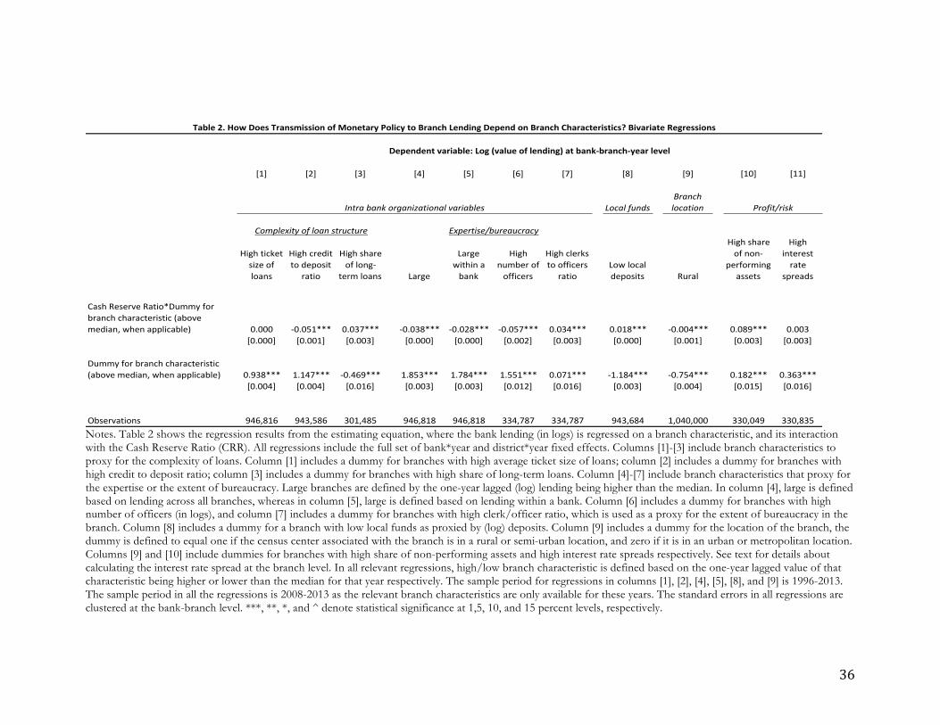
! 36!

!Notes. Table 2 shows the regression results from the estimating equation, where the bank lending (in logs) is regressed on a branch characteristic, and its interaction with the Cash Reserve Ratio (CRR). All regressions include the full set of bank*year and district*year fixed effects. Columns [1]-[3] include branch characteristics to proxy for the complexity of loans. Column [1] includes a dummy for branches with high average ticket size of loans; column [2] includes a dummy for branches with high credit to deposit ratio; column [3] includes a dummy for branches with high share of long-term loans. Column [4]-[7] include branch characteristics that proxy for the expertise or the extent of bureaucracy. Large branches are defined by the one-year lagged (log) lending being higher than the median. In column [4], large is defined based on lending across all branches, whereas in column [5], large is defined based on lending within a bank. Column [6] includes a dummy for branches with high number of officers (in logs), and column [7] includes a dummy for branches with high clerk/officer ratio, which is used as a proxy for the extent of bureaucracy in the branch. Column [8] includes a dummy for a branch with low local funds as proxied by (log) deposits. Column [9] includes a dummy for the location of the branch, the dummy is defined to equal one if the census center associated with the branch is in a rural or semi-urban location, and zero if it is in an urban or metropolitan location. Columns [9] and [10] include dummies for branches with high share of non-performing assets and high interest rate spreads respectively. See text for details about calculating the interest rate spread at the branch level. In all relevant regressions, high/low branch characteristic is defined based on the one-year lagged value of that characteristic being higher or lower than the median for that year respectively. The sample period for regressions in columns [1], [2], [4], [5], [8], and [9] is 1996-2013. The sample period in all the regressions is 2008-2013 as the relevant branch characteristics are only available for these years. The standard errors in all regressions are clustered at the bank-branch level. ***, **, *, and ^ denote statistical significance at 1,5, 10, and 15 percent levels, respectively.

[1] [2] [3] [4] [5] [6] [7] [8] [9] [10] [11]

Local&fundsBranch&location

High1ticket1

size1of1

loans

High1credit1

to1deposit1

ratio

High1share1

of1long@

term1loans Large1

Large11

within1a1

bank

High1

number1of1

officers

High1clerks1

to1officers1

ratio

Low1local1

deposits Rural

High1share1

of1non@

performing1

assets

High1

interest1

rate1

spreads

Cash1Reserve1Ratio*Dummy1for1

branch1characteristic1(above1

median,1when1applicable) 0.000 @0.051*** 0.037*** @0.038*** @0.028*** @0.057*** 0.034*** 0.018*** @0.004*** 0.089*** 0.003

[0.000] [0.001] [0.003] [0.000] [0.000] [0.002] [0.003] [0.000] [0.001] [0.003] [0.003]

Dummy1for1branch1characteristic1

(above1median,1when1applicable) 0.938*** 1.147*** @0.469*** 1.853*** 1.784*** 1.551*** 0.071*** @1.184*** @0.754*** 0.182*** 0.363***

[0.004] [0.004] [0.016] [0.003] [0.003] [0.012] [0.016] [0.003] [0.004] [0.015] [0.016]

Observations 946,816 943,586 301,485 946,818 946,818 334,787 334,787 943,684 1,040,000 330,049 330,835

Table&2.&How&Does&Transmission&of&Monetary&Policy&to&Branch&Lending&Depend&on&Branch&Characteristics?&Bivariate&Regressions

Intra&bank&organizational&variables

Dependent&variable:&Log&(value&of&lending)&at&bankGbranchGyear&level

Profit/risk

Complexity&of&loan&structure Expertise/bureaucracy

! 37!

!Notes. Table 3 shows the regression results from the estimating equation, where the bank lending (in logs) is regressed on several branch characteristics, and their interactions with the Cash Reserve Ratio (CRR). All regressions include the full set of bank*year and district*year fixed effects. See notes to Table 2 for details of the branch characteristics. The coefficients on the branch characteristics (without the interaction with CRR) are not shown in the table for brevity. The sample period in all the regressions is 2008-2013. The standard errors in all regressions are clustered at the bank-branch level. ***, **, *, and ^ denote statistical significance at 1,5, 10, and 15 percent levels, respectively.

!

Intra&bank&organizational&variablesCash%Reserve%Ratio*Branch%with%high%ticket%size%loans 0.039***

[0.003]

Cash%Reserve%Ratio*Branch%with%high%credit%to%deposit%ratio >0.033***

[0.002]

Cash%Reserve%Ratio*Branch%with%high%share%of%long>term%loans 0.027***

[0.002]

Cash%Reserve%Ratio*Branch%with%high%number%of%officers >0.099***

[0.002]

Local&fundsCash%Reserve%Ratio*Branch%with%low%deposits 0.011***

[0.003]

Geographical&locationCash%Reserve%Ratio*Rural%branch% >0.006**

[0.002]

Profits/RiskCash%Reserve%Ratio*High%interest%rate%spreads 0.047***

[0.002]

Cash%Reserve%Ratio*Branch%with%high%share%of%non>performing%assets 0.026***

[0.002]

Table&3.&How&Does&Transmission&of&Monetary&Policy&to&Branch&Lending&Depend&on&Branch&Characteristics?&Multivariate&Regressions

Dependent&variable:&Log&(value&of&lending)&at&bankGbranchGyear&level

! 38!

!Notes. Table 4 shows the regression results from the estimating equation, where the bank lending (in logs) is regressed on the CRR, several branch characteristics, and their interactions with the CRR. All regressions include the full set of bank and district fixed effects. Importantly, year fixed effects are dropped so as to allow include the CRR (without the interaction) in the regression. See notes to Table 2 for details of the branch characteristics. The coefficients on the branch characteristics (without the interaction with CRR) are not shown in the table for brevity. The sample period in all the regressions is 2008-2013. The standard errors in all regressions are clustered at the bank-branch level. ***, **, *, and ^ denote statistical significance at 1,5, 10, and 15 percent levels, respectively.

Cash%Reserve%Ratio -0.210***[0.004]

Intra&bank&organizational&variablesCash%Reserve%Ratio*Branch%with%high%ticket%size%loans 0.052***

[0.002]

Cash%Reserve%Ratio*Branch%with%high%credit%to%deposit%ratio -0.047***

[0.002]

Cash%Reserve%Ratio*Branch%with%high%share%of%long-term%loans 0.037***

[0.002]

Cash%Reserve%Ratio*Branch%with%high%number%of%officers -0.035***

[0.003]

Local&fundsCash%Reserve%Ratio*Branch%with%low%deposits 0.014***

[0.003]

Geographical&locationCash%Reserve%Ratio*Rural%branch% -0.016***

[0.003]

Profits/riskCash%Reserve%Ratio*High%interest%rate%spreads 0.050***

[0.002]

Cash%Reserve%Ratio*Branch%with%high%share%of%non-performing%assets 0.025***

[0.002]

Table&4.&Transmission&of&Monetary&Policy&to&Branch&Lending.&Overall&Effect

Dependent&variable:&Log&(value&of&lending)&at&bankDbranchDyear&level

! 39!

!Notes. Table 5 repeats the regression in Table 3 for the branches of state-owned and private banks separately. All regressions include the full set of bank and district fixed effects. See notes to Table 2 for details of the branch characteristics. The coefficients on the branch characteristics (without the interaction with CRR) are not shown in the table for brevity. The sample period in all the regressions is 2008-2013. The standard errors in all regressions are clustered at the bank-branch level. ***, **, *, and ^ denote statistical significance at 1,5, 10, and 15 percent levels, respectively.

!

[1] [2]State%Owned*Banks Private*Banks

Intra&bank&organizational&variablesCash)Reserve)Ratio*Branch)with)high)ticket)size)loans 0.023*** 0.152***

[0.002] [0.016]

Cash)Reserve)Ratio*Branch)with)high)credit)to)deposit)ratio A0.024*** A0.080***

[0.002] [0.012]

Cash)Reserve)Ratio*Branch)with)high)share)of)longAterm)loans 0.023*** 0.086***

[0.002] [0.015]

Cash)Reserve)Ratio*Branch)with)high)number)of)officers A0.090*** A0.155***

[0.002] [0.015]

Local&fundsCash)Reserve)Ratio*Branch)with)low)deposits 0.010*** 0.010

[0.003] [0.013]

Geographical&locationCash)Reserve)Ratio*Rural)branch) A0.028*** 0.111***

[0.002] [0.014]

Profits/riskCash)Reserve)Ratio*High)interest)rate)spreads 0.042*** 0.074***

[0.002] [0.019]Cash)Reserve)Ratio*Branch)with)high)share)of)nonAperforming)assets 0.003 0.208***

[0.002] [0.013]

Table*5.*How*Does*Transmission*of*Monetary*Policy*to*Branch*Lending*Depend*on*Branch*Characteristics?*State%Owned*and*Private*Banks

Dependent*variable:*Log*(value*of*lending)*at*bank%branch%year*level

! 40!

!Notes. Table 6 repeats the regression in Table 3 for episodes of tightening and loosening of monetary policy separately. Episode of tightening and loosening are defined as years when the CRR was increased and reduced respectively. All regressions include the full set of bank and district fixed effects. See notes to Table 2 for details of the branch characteristics. The coefficients on the branch characteristics (without the interaction with CRR) are not shown in the table for brevity. The sample period in all the regressions is 2008-2013. The standard errors in all regressions are clustered at the bank-branch level. ***, **, *, and ^ denote statistical significance at 1,5, 10, and 15 percent levels, respectively.

[1] [2]Tightening Loosening

Intra&bank&organizational&variablesCash)Reserve)Ratio*Branch)with)high)ticket)size)loans :0.334*** 0.063***

[0.058] [0.007]

Cash)Reserve)Ratio*Branch)with)high)credit)to)deposit)ratio 0.222*** :0.106***

[0.046] [0.006]

Cash)Reserve)Ratio*Branch)with)high)share)of)long:term)loans :0.192*** 0.045***

[0.055] [0.006]

Cash)Reserve)Ratio*Branch)with)high)number)of)officers 0.191*** :0.125***

[0.057] [0.006]

Local&fundsCash)Reserve)Ratio*Branch)with)low)deposits :0.173*** 0.055***

[0.059] [0.007]

Geographical&locationCash)Reserve)Ratio*Rural)branch) 0.009 :0.031***

[0.051] [0.007]

Profits/riskCash)Reserve)Ratio*High)interest)rate)spreads :0.176*** :0.009

[0.061] [0.006]

Cash)Reserve)Ratio*Branch)with)high)share)of)non:performing)assets :0.223*** :0.016**

[0.056] [0.006]

Table.6..How.Does.Transmission.of.Monetary.Policy.to.Branch.Lending.Depend.on.Branch.Characteristics?.Episodes.of.Tightening.and.Loosening

Dependent.variable:.Log.(value.of.lending).at.bankGbranchGyear.level

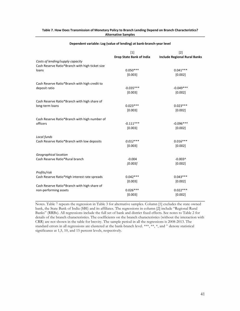
! 41

!Notes. Table 7 repeats the regression in Table 3 for alternative samples. Column [1] excludes the state owned bank, the State Bank of India (SBI) and its affiliates. The regressions in column [2] include “Regional Rural Banks” (RRBs). All regressions include the full set of bank and district fixed effects. See notes to Table 2 for details of the branch characteristics. The coefficients on the branch characteristics (without the interaction with CRR) are not shown in the table for brevity. The sample period in all the regressions is 2008-2013. The standard errors in all regressions are clustered at the bank-branch level. ***, **, *, and ^ denote statistical significance at 1,5, 10, and 15 percent levels, respectively.

! !

[1] [2]Drop%State%Bank%of%India Include%Regional%Rural%Banks

Costs%of%lending/supply%capacityCash)Reserve)Ratio*Branch)with)high)ticket)size)loans 0.050*** 0.041***

[0.003] [0.002]

Cash)Reserve)Ratio*Branch)with)high)credit)to)deposit)ratio A0.035*** A0.049***

[0.003] [0.002]

Cash)Reserve)Ratio*Branch)with)high)share)of)longAterm)loans 0.023*** 0.023***

[0.003] [0.002]

Cash)Reserve)Ratio*Branch)with)high)number)of)officers A0.111*** A0.096***

[0.003] [0.002]

Local%fundsCash)Reserve)Ratio*Branch)with)low)deposits 0.012*** 0.016***

[0.003] [0.002]

Geographical%locationCash)Reserve)Ratio*Rural)branch) A0.004 A0.003^

[0.003] [0.002]

Profits/riskCash)Reserve)Ratio*High)interest)rate)spreads 0.042*** 0.043***

[0.003] [0.002]Cash)Reserve)Ratio*Branch)with)high)share)of)nonAperforming)assets 0.026*** 0.022***

[0.003] [0.002]

Table%7.%How%Does%Transmission%of%Monetary%Policy%to%Branch%Lending%Depend%on%Branch%Characteristics?%Alternative%Samples

Dependent%variable:%Log%(value%of%lending)%at%bankJbranchJyear%level

! 42

Notes. Table 8 checks the robustness of the regression in Table 3 to omitted variables. Column [1] includes a dummy for year in which state elections took place, and the interaction of this dummy with the rural dummy. Column [2] includes the interactions of the all branch characteristics with another macro variable - the inflation rate. All regressions include the full set of bank and district fixed effects. See notes to Table 2 for details of the branch characteristics. The coefficients on the branch characteristics (without the interaction with CRR) are not shown in the table for brevity. The sample period in all the regressions is 2008-2013. The standard errors in all regressions are clustered at the bank-branch level. ***, **, *, and ^ denote statistical significance at 1,5, 10, and 15 percent levels, respectively.

! !

[1] [2]

Elections Other-macroeconomic-variablesCosts%of%lending/supply%capacityCash)Reserve)Ratio*Branch)with)high)ticket)size)loans 0.039*** 0.044***

[0.003] [0.003]

Cash)Reserve)Ratio*Branch)with)high)credit)to)deposit)ratio A0.033*** A0.036***

[0.002] [0.002]

Cash)Reserve)Ratio*Branch)with)high)share)of)longAterm)loans 0.027*** 0.030***

[0.002] [0.002]

Cash)Reserve)Ratio*Branch)with)high)number)of)officers A0.099*** A0.104***

[0.002] [0.002]

Local%fundsCash)Reserve)Ratio*Branch)with)low)deposits 0.011*** 0.012***

[0.003] [0.003]

Geographical%locationCash)Reserve)Ratio*Rural)branch) A0.007*** A0.008***

[0.002] [0.003]

Profits/riskCash)Reserve)Ratio*High)interest)rate)spreads 0.047*** 0.047***

[0.002] [0.002]Cash)Reserve)Ratio*Branch)with)high)share)of)nonAperforming)assets 0.026*** 0.026***

[0.002] [0.002]

Table-8.-How-Does-Transmission-of-Monetary-Policy-to-Branch-Lending-Depend-on-Branch-Characteristics?-Omitted-Variables

Dependent-variable:-Log-(value-of-lending)-at-bankIbranchIyear-level

! 43

Notes. Table 9 checks the robustness of the regression in Table 3 to omitted variables. Column [1] includes the interactions of the all branch characteristics with the policy repo rate. Column [2] includes the interactions of the all branch characteristics with the policy repo rate and the statutory liquidity ratio (SLR). All regressions include the full set of bank and district fixed effects. See notes to Table 2 for details of the branch characteristics. The coefficients on the branch characteristics (without the interaction with CRR) are not shown in the table for brevity. The sample period in all the regressions is 2008-2013. The standard errors in all regressions are clustered at the bank-branch level. ***, **, *, and ^ denote statistical significance at 1,5, 10, and 15 percent levels, respectively.

!! !

[1] [2]

Costs%of%lending/supply%capacityCash%Reserve%Ratio*Branch%with%high%ticket%size%loans 0.022*** 0.045***

[0.003] [0.005]

Cash%Reserve%Ratio*Branch%with%high%credit%to%deposit%ratio @0.020*** @0.032***

[0.002] [0.004]

Cash%Reserve%Ratio*Branch%with%high%share%of%long@term%loans 0.021*** 0.028***

[0.002] [0.005]

Cash%Reserve%Ratio*Branch%with%high%number%of%officers @0.081*** @0.132***

[0.002] [0.005]

Local%fundsCash%Reserve%Ratio*Branch%with%low%deposits 0.004 0.002

[0.002] [0.005]

Geographical%locationCash%Reserve%Ratio*Rural%branch% @0.001 @0.027***

[0.002] [0.005]

Profits/riskCash%Reserve%Ratio*High%interest%rate%spreads 0.055*** 0.011**

[0.003] [0.005]Cash%Reserve%Ratio*Branch%with%high%share%of%non@performing%assets 0.034*** @0.021***

[0.002] [0.005]

Table*9.*How*Does*Transmission*of*Monetary*Policy*to*Branch*Lending*Depend*on*Branch*Characteristics?*Omitted*Variables*(contd)

Dependent*variable:*Log*(value*of*lending)*at*bankLbranchLyear*level

! 44

Notes. Table 10 checks the robustness of the regression in Table 3 to alternative specifications. Column [1] includes the interactions of the all branch characteristics with one-year lagged CRR. Column [2] includes the first difference of log(lending) as the dependent variable, and the interactions of the all branch characteristics with the first difference of CRR. Column [3] repeats the specification in Table 3 by including a lagged dependent variable in the model. All regressions include the full set of bank and district fixed effects. See notes to Table 2 for details of the branch characteristics. The coefficients on the branch characteristics (without the interaction with CRR) are not shown in the table for brevity. The sample period in all the regressions is 2008-2013. The standard errors in all regressions are clustered at the bank-branch level. ***, **, *, and ^ denote statistical significance at 1,5, 10, and 15 percent levels, respectively. !

!

[1] [2] [3]One)year-lagged-CRR First-difference-in-lending-and- Lagged-dependent-variable

Dependent'variable:'Log'(value'of'lending)'at'bank7

branch7year'levelFirst'difference'of'Log'(value'of'lending)'at'bank7branch7year'

Log'(value'of'lending)'at'bank7branch7year'level

Intra&bank&organizational&variablesCash-Reserve-Ratio*Branch-with-high-ticket-size-loans 0.052*** 0.009*** 0.027***

[0.002] [0.001] [0.002]

Cash-Reserve-Ratio*Branch-with-high-credit-to-deposit-ratio )0.036*** )0.007*** )0.002*

[0.001] [0.001] [0.001]

Cash-Reserve-Ratio*Branch-with-high-share-of-long)term-loans 0.012*** 0.001 0.009***

[0.002] [0.001] [0.001]

Cash-Reserve-Ratio*Branch-with-high-number-of-officers )0.027*** )0.013*** )0.025***

[0.002] [0.001] [0.001]

Local&fundsCash-Reserve-Ratio*Branch-with-low-deposits 0.010*** 0.009*** )0.012***

[0.002] [0.001] [0.002]

Geographical&locationCash-Reserve-Ratio*Rural-branch- 0.056*** )0.006*** )0.034***

[0.002] [0.001] [0.002]

Profits/RiskCash-Reserve-Ratio*High-interest-rate-spreads )0.027*** )0.004*** 0.018***

[0.002] [0.001] [0.001]

Cash-Reserve-Ratio*Branch-with-high-share-of-non)performing-assets )0.022*** )0.010*** 0.010***

[0.002] [0.001] [0.001]

Table'10.'How'Does'Transmission'of'Monetary'Policy'to'Branch'Lending'Depend'on'Branch'Characteristics?'Dynamic'Specifications

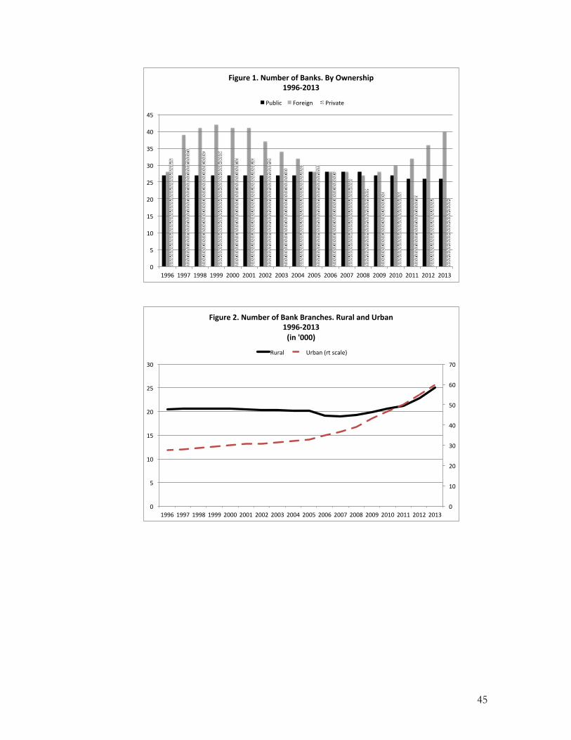
! 45

!!

!!

0"

5"

10"

15"

20"

25"

30"

35"

40"

45"

1996" 1997" 1998" 1999" 2000" 2001" 2002" 2003" 2004" 2005" 2006" 2007" 2008" 2009" 2010" 2011" 2012" 2013"

Figure'1.'Number'of'Banks.'By'Ownership'1996;2013''

Public" Foreign"" Private"

0"

10"

20"

30"

40"

50"

60"

70"

0"

5"

10"

15"

20"

25"

30"

1996" 1997" 1998" 1999" 2000" 2001" 2002" 2003" 2004" 2005" 2006" 2007" 2008" 2009" 2010" 2011" 2012" 2013"

Figure'2.'Number'of'Bank'Branches.'Rural'and'Urban'1996=2013'(in''000)'

Rural"" Urban"(rt"scale)"

! 46

!!

!!!

!!

! !

0"

10"

20"

30"

40"

50"

60"

1996"1997"1998"1999"2000"2001"2002"2003"2004"2005"2006"2007"2008"2009"2010"2011"2012"2013"

In#percent#

Figure#3.#Share#of#Bank#Lending.#By#Ownership#1996?2013##

SBI"Group" Foreign"" Regional"Rural" Private" Other"Public"

0"

50"

100"

150"

200"

250"

300"

350"

400"

0.0"

0.5"

1.0"

1.5"

2.0"

2.5"

3.0"

3.5"

1996"1997"1998"1999"2000"2001"2002"2003"2004"2005"2006"2007"2008"2009"2010"2011"2012"2013"

Figure'4.'Value'of'Lending.'Rural'and'Urban'Branches.''1996<2013'

(in''000'crores'of'rupees)'Rural" Urban"(rt"scale)"

! 47

!!

!!

0"

100"

200"

300"

400"

500"

600"

700"

800"

900"

0"

50"

100"

150"

200"

250"

300"

350"

1996"1997"1998"1999"2000"2001"2002"2003"2004"2005"2006"2007"2008"2009"2010"2011"2012"2013"

Figure'5.'Number'of'Loans.'Rural'and'Urban'Branches'1996=2013'

(in'lakhs,'or'100,000)'

Rural" Urban"(rt"scale)"

0"

100"

200"

300"

400"

500"

600"

700"

0"

20"

40"

60"

80"

100"

120"

140"

1996" 1997" 1998" 1999" 2000" 2001" 2002" 2003" 2004" 2005" 2006" 2007" 2008" 2009" 2010" 2011" 2012" 2013"

Figure'6.'Average'Ticket'Size.'Rural'and'Urban'Branches'1996>2013'

(in''000'of'rupees)'

Rural" Urban"(rt"scale)"

! 48

!!

!!

0"

10"

20"

30"

40"

50"

60"

70"

80"

90"

100"

0"

500"

1000"

1500"

2000"

2500"

3000"

3500"

1996"1997"1998"1999"2000"2001"2002"2003"2004"2005"2006"2007"2008"2009"2010"2011"2012"2013"

In#percent#

Inde

x#

Figure#7.#Bank#Concentra6on#at#the#District#Level.##1996@2013#

Average"Herfindahl"Index"of"Bank"ConcentraAon"of"Credit""

Average"Share"of"Top"4"Banks"in"Total"Credit"(right"scale)"

0"

500"

1000"

1500"

2000"

2500"

3000"

1996" 1997" 1998" 1999" 2000" 2001" 2002" 2003" 2004" 2005" 2006" 2007" 2008" 2009" 2010" 2011" 2012" 2013"

Figure'8.'Bank'Concentra2on.'Rural'and'Urban'Branches'1996=2013'

Rural" Urban"

! 49

!!!

!!!

!!

! !

15#

17#

19#

21#

23#

25#

27#

29#

31#

33#

0#

2#

4#

6#

8#

10#

12#

14#

16#

4/27/96#

4/27/97#

4/27/98#

4/27/99#

4/27/00#

4/27/01#

4/27/02#

4/27/03#

4/27/04#

4/27/05#

4/27/06#

4/27/07#

4/27/08#

4/27/09#

4/27/10#

4/27/11#

4/27/12#

4/27/13#

4/27/14#

Figure'9.'Monetary'Policy:'Quan5ty'Instruments.''1996;2013'

Cash#Reserve#Ra5o# Statutory#Liquidity#Ra5o#(right#axis)#

0"

1"

2"

3"

4"

5"

6"

7"

8"

9"

10"

12/29/01" 12/29/02" 12/29/03" 12/29/04" 12/29/05" 12/29/06" 12/29/07" 12/29/08" 12/29/09" 12/29/10" 12/29/11" 12/29/12" 12/29/13"

Figure'10.'Monetary'Policy:'Rate'Instruments.'1996;2013''

repo" reverse"repo"

! 50

!!!

!!!!!

20#

25#

30#

35#

40#

45#

50#

4#

5#

6#

7#

8#

9#

10#

4/27/96#

4/27/97#

4/27/98#

4/27/99#

4/27/00#

4/27/01#

4/27/02#

4/27/03#

4/27/04#

4/27/05#

4/27/06#

4/27/07#

4/27/08#

4/27/09#

4/27/10#

4/27/11#

4/27/12#

4/27/13#

4/27/14#

Figure'11.'Monetary'Policy:'Quan5ty'and'Price'Instruments.'1996<2013''

policy#rate# quan:ty#(right#scale)#