the transparent prolog machine (tpm): an …
TRANSCRIPT
J. LOGIC PROGRAMMING 1988:5:277-342 271
THE TRANSPARENT PROLOG MACHINE (TPM): AN EXECUTION MODEL AND GRAPHICAL DEBUGGER FOR LOGIC PROGRAMMING*
MARC EISENSTADT AND MIKE BRAYSHAW
D An augmented AND/OR tree representation of logic programs is presented as the basis for an advanced graphical tracing and debugging facility for PROLOG. An extension of our earlier work on “retrospective zooming”, this representation offers several distinct advantages over existing tracing and debugging facilities: (1) it naturally incorporates traditional AND/OR
trees and Byrd box models (call/exit/fail/redo procedural models) as special cases; (2) it can be run in slow-motion, close-up mode for novices or high-speed, long-distance mode for experts with no attendant conceptual change; (3) it serves as the uniform basis for textbook material, video-based teaching material, and an advanced user interface for experienced PROLOG programmers; (4) it tells the truth about clause head matching and deals correctly with the cut. One of the key insights underlying the work is the realization that it is possible to display an execution space of several thousand nodes in a meaningful way on a modem graphics workstation. By enhancing AND/OR trees to include “status boxes” rather than simple “nodes”, it is possible to display both a long-distance view of execution and the full details of clause-head matching. Graphical “collapsing” techniques enable the model to deal with user-defined abstractions, higher-order predi- cates such as setof, and definite-clause grammars. The current implementa- tion runs on modern graphics workstations and is written in PROLOG. a
1. INTRODUCTION
The need for clear and consistent models of program execution has received great attention not only from the human-computer interaction community (e.g. [7]), but also from the software engineering and AI communities (e.g. [18,24,25]). The
Address correspondence to Marc Eisenstadt, Human Cognition Research Laboratory, The Open University, Milton Keynes MK7 6AA, U.K.
Received 20 December 1986; accepted 23 October 1987. *We gratefully acknowledge the support of the U.K. Science and Engineering Research Council
(grant nos. GR/C/69344 and GR/E/2333.3). Work is continuing on this project under an Alvey research contract shared with Expert Systems International, Ltd.
THE JOURNAL OF LOGIC PROGRAMMING
QElsevier Science Publishing Co., Inc., 1938
655 Ave. of the Americas, New York, NY 10010 0743-1066/88/$3.50
278 MARCEISENSTADTANDMIKEBRAYSHAW
benefits of such models are both pedagogical and practical: the whole development/debugging cycle can be streamlined when the programmer is equipped with facilities for clearly visualizing and monitoring program execution.
Logic programming is no exception, although to date most of the emphasis on debugging logic programs has been placed either on a deep understanding of the declarative semantics (e.g. [26,21,16]) or reasoning about the rationale underlying the debugging process [20]. Attempts to build software engineering environments in which PROLOG is embedded (e.g. [15,13]) have resulted in facilities which encour- age a clean top-down programming style reinforced either by shell commands or by a syntax-directed editor, but which are nevertheless strongly wedded to the “glass- teletype” environment in which they were conceived. Despite the import of these studies, PROLOG programmers today are still confined in their daily practice to a rather tedious view of program execution obtained by using the built-in “spy” trace packages available in most implementations. Our belief is that declarative debug-
ging can most fruitfully be incorporated within the scope of a larger logic-program- ming environment such as that proposed in the remainder of this paper. We concentrate on the procedural side of PROLOG, because (for better or worse) that is the weak link in the program development and debugging cycle for both new students and experienced users, and therefore is worthy of at least some short-term remedial attention.
Bundy and his colleagues at the University of Edinburgh have provided an excellent account of the many tradeoffs involved in trying to develop a good “PROLOG story” which could be used both for teaching PROLOG and for providing a view of execution in the context of writing and debugging large PROLOG programs [l, 191. The basic tenet of the “Edinburgh Stories” school, as we shall call it, is that an AND/OR tree provides the best overall account of what is happening during PROLOG execution, but that it needs to be combined with a view of the database and a resolution table to explicate the links to the user’s original code and to the all-important variable instantiations which occur during execution. The Edinburgh Stories account argues that although there is not normally enough room to show the execution of very large programs, this might be possible through the principled use of multiple-window displays.
The problem of designing a purpose-built graphical tracer for PROLOG pro- grams was addressed by Dewar and Cleary [8]. Their system attempts to provide an intuitive “zooming” facility for examining PROLOG execution in detail. Although it incorporates a very nice display of clause-head selection and the active goal-sub- goal hierarchy, it suffers from four deficiencies:
(1)
(2)
Every goal invocation involves a complete replication of the icons depicting the relevant portion of the database. Although zooming techniques can render these very small, the space they occupy rapidly grows out of all proportion to their importance in understanding the behavior of the running program. For example, the execution of a simple grandfather&Y) example (eight facts, two rules) fills the screen, whereas a practical tracer needs to be able to display thousands of nodes at a time and have them meaningfully visible.
The logical structure of the AND/OR tree, acknowledged by Dewar and Clear-y to be important, is sacrificed for practical reasons. It is a commonly held view that an AND/OR tree would be “nice”, but that it is “too

THE TRANSPARENT PROLOG MACHINE 279
(3)
(4)
impractical”. Below we show how our notation overcomes such practical restrictions, thereby maintaining the logical clarity of an AND/OR tree.
The mapping between the user’s source code and the running invocations is sacrificed in order to provide a concise display, including user-defined icons. This is a difficult tradeoff. The user-defined aspects of the display are very important, but we feel that it is critical to have the terms which appear in the display reflect precisely the terms which the user wrote in the original program.
The actual implementation runs too slowly to be used on anything other than “toy” examples. Although we are in complete sympathy with the need to
pursue important theoretical and design issues within the realms of small test examples, we feel very strongly that solutions to toy problems simply do not scale up to the enormous size of serious logic-programming applications. Large-scale problems are themselves therefore of fundamental importance to work of the type described herein.
Rajan’s work [23] is an inspiring attempt to “Cell the truth” about PROLOG execution, and to do so in a way which conforms to the way the user has written his or her own code. Rajan’s single-stepper works its way through code by highlighting relevant portions in the database at the appropriate moments, and by instantiating clause bodies in their entirety “in place” in the code being traced. By showing unification in painstaking detail, a clear account of execution can be presented to novices. However, Rajan’s single-stepper doesn’t fully show variable renaming. Although this was not necessary for the class of beginners he was addressing, it is essential for users of the system we are developing. Moreover, the execution spaces for such a textually derived system are inherently small. Our efforts at displaying “slow motion” unification are analogous to (and influenced by) Rajan’s, but we depart from his emphasis (1) on textually derived displays and (2) the need to highlight source code in its original edit window. Regarding (l), we move strongly in the direction of high-resolution graphical displays to show “execution space” trees. As far as (2) is concerned, we leave it up to the user to inspect source code (in an on-screen window, if so desired), and instead allow inspection of the detailed aspects of unification by user-initiated request at specific nodes in the execution tree.
Our own earlier work [lo, 111 and the work of Plummer [22] concentrated on enhancing the “Byrd box” execution model [3] to the point where it would give more precise symptomatic information so that the programmer could home in more readily on trouble spots. In [ll] we added a top-level supervisory program which could detect characteristic “symptom clusters” produced behind the scenes by the trace package in order to spot bugs. The current effort is an attempt to provide a significant boost to the practical debugging of very large programs by highly experienced PROLOG programmers. The underlying philosophy of “retrospective zooming” introduced in [ll] still applies, but now we apply the modern graphical techniques which the earlier work only hinted at. Moreover, our approach incorpo- rates ideas gained from teaching introductory PROLOG, and thereby provides facilities in a clear and consistent manner so that they are useful to experts and novices alike.
The work described herein starts with two premises: (1) it is essential to show the full execution space of large PROLOG programs; (2) it is essential to base a tracing
280 MARCEISENSTADTANDMIKEBRAYSHAW
package on an “extended execution model” which discriminates between clause-head matching and clause-body execution. We have stuck with these two premises, partly because of the challenge of resolving their underlying contradiction: premise (1) involves a global view of things, while premise (2) involves a very close-up view. Our aim has been to reconcile these differences without losing the advantages provided by either premise. We feel strongly that different levels of detail (i.e. different grain sizes of analysis) involve different conceptual views of what is happening, and therefore a simple “aerial view/close-up zoom” facility (such as that used in the tracer of [8]) does not provide a magical solution, particularly when programs other than toy examples are involved. It is nevertheless possible to accommodate both premises. The key insights which enable this accommodation, and which drive the whole of the work described in this paper, are the following:
It is possible to display an execution space involving thousands of nodes on today’s graphics workstations.
When a PROLOG programmer is debugging a program which he or she has
personally been developing over a period of weeks or months, an overall graphical view of the execution space of that program is highly meaningful to that programmer, because it conveys its own gestalt. (We have a strong hunch that this is true up to a limit of several thousand nodes, although this needs to be tested empirically.)
The concept of a “node” in a traditional AND/OR tree is needlessly impover- ished. With just a few enhancements, and for a very small computational overhead, a simple node can become a “status box” which concisely encapsu- lates a goal’s history, including detailed clause-head matching information.
The traditional AND/OR tree does not reveal the difference between one clause containing a disjunction and two separate clauses. More specifically, the distinction between clause head and clause body is not shown in AND/ OR
trees, despite the overwhelming importance of the head/body distinction in the debugging of PROLOG programs. A minor notational variant enables us
to overcome this problem.
Section 2 describes the underlying principles involved in the design and develop- ment of our view of PROLOG execution, which we dub the “transparent PROLOG machine” (TPM). TPM serves as the basis for our own textbook and video material [12] as well as providing the underlying execution model for our graphics tracer. To illustrate TPM notation, test cases taken from Pain and Bundy [19], Bundy et al. [1,2], and Coombs and Stell [6] are presented. Details of the running user environ- ment are presented in Section 3. Section 4 presents a series of worked examples, namely, a small expert system, a database manipulation program, and a simple programming-language compiler. Section 5 discusses TPM extensions to deal with abstractions such as setof and definite-clause grammars. Concluding remarks are given in Section 6. The account which follows presupposes that the reader is an experienced PROLOG user.
2. THE TRANSPARENT PROLOG MACHINE: UNDERLYING PRINCIPLES
In this section we describe an idealized account of PROLOG execution. Our work differs from the Edinburgh Stories school in three important respects: (1) in our
THE TRANSPARENT PROLOG MACHINE 281
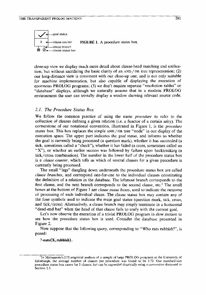
clause counter FIGURE 1. A procedure status box.
close-up view we display much more detail about clause-head matching and unifica- tion, but without sacrificing the basic clarity of an AND/OR tree representation; (2) our long-distance view is consistent with our close-up one, and is not only suitable for machine implementation, but also capable of displaying the execution of enormous PROLOG programs; (3) we don’t require separate “resolution tables” or “database” displays, although we naturally assume that in a modem PROLOG environment the user can trivially display a window showing relevant source code.
2.1. The Procedure Status Box
We follow the common practice of using the name procedure to refer to the collection of clauses defining a given relation (i.e. a functor of a certain arity). The cornerstone of our notational convention, illustrated in Figure 1, is the procedure status box. This box replaces the simple AND/OR tree “node” in our display of the execution space. The upper part indicates the goal status, and informs us whether the goal is currently being processed (a question mark), whether it has succeeded (a tick, sometimes called a “check”), whether it has failed (a cross, sometimes called an “X”), or whether an earlier success was followed by failure upon backtracking (a tick/cross combination). The number in the lower half of the procedure status box is a clause counter, which tells us which of several clauses for a given procedure is currently being processed.
The small “legs” dangling down underneath the procedure status box are called clause branches, and correspond one-for-one to the individual clauses constituting the definition of a relation in the database. The leftmost branch corresponds to the first clause, and the next branch corresponds to the second clause, etc.’ The small boxes at the bottom of Figure 1 are clause status boxes, used to indicate the outcome of processing of each individual clause. The clause status box may contain any of the four symbols used to indicate the main goal status (question mark, tick, cross, and tick/cross). Alternatively, a clause branch may simply terminate in a horizontal “dead-end bar” when the head of that clause fails to unify with the current goal.
Let’s now observe the execution of a trivial PROLOG program in slow motion to see how the procedure status box is used. Consider the database presented in Figure 2.
Now suppose that the following query, corresponding to “Who eats rubbish?“, is posed:
?-eats(X, rubbish).
‘In Matsumoto’s [17] empirical analysis of a sample of large PROLOG programs at the University of Edinburgh, the average number of clauses per procedure was found to be 3.72. Our standard-size procedure status box caters for 5 clauses, but can be expanded drastically using a convention discussed in Section 2.3.

282 MARC EISENSTADT AND MIKE BRAYSHAW
eats(joe, hamburgers). eats(fred,X). 5% fred eats anything eats& bread). % everyone (actualIy anything) eats bread
FIGURE 2. Three clauses defining eats.
Figure 3(a)-(d) show the “innards” of execution. In Figure 3(a), we see the main goal displayed alongside the procedure status box. The goal status symbol is a
question mark, there are three clause branches corresponding to the clauses in the definition of eats, and the “0” indicates that no clauses have yet been inspected. Whenever a clause is inspected, it is first copied, and any variables are renamed by adding an appropriately numbered subscript. Then an attempt is made to unify the head of that clause with the current goal. Figure 3(b) depicts the moment when clause 1 of eats is inspected. The head of this clause fails to unify with the current goal, so the first clause branch has just been marked with a horizontal dead-end bar. Next, clause 2 is inspected, as shown in Figure 3(c). There are three important things to note even in this simple example. Firstly, in the copy of clause 2 being inspected, the variable X has been appropriately renamed by adding a subscript, so that X, is distinct from the X in the query (which is, in essence, X,). Secondly, the arrows in Figure 3(c) are unification arrows which form an intrinsic part of our execution model. They indicate not only that X is instantiated to fred and X, is instantiated to rubbish, but also (at a glance) that X is an output variable and Xi is an input variable. Thirdly, the clause status box at this instant has a question mark in it, meaning that the interpreter technically needs to pursue the body of this clause. We can see that the clause is an ordinary PROLOG fact, and therefore appears to have no body, but more formally it actually has the implicit body true, which is trivially satisfiable. If there had been one or more subgoals in the body,
eals(X , rubbish )
eats(X , rubbish )
eats(joe , hamburgers)
eats(fred , X, )
eats(X , rubbish )
eats(fred , X, )
FIGURE 3. Four-step detailed execution snapshots, given the new query ?- eats(X,rubbish): (a) Initial pending goal. (b) A copy of clause 1 of eats is inspected, but the head does not unify with the goal. (c) A copy of clause 2 is inspected, and its head does unify, as shown. Variables in clauses which are copied and inspected are automatically renamed by adding an appropriately numbered subscript. At this instant, the interpreter does not know that clause 2 is a winner. (d) End of processing. The clause status box for clause 2 shows that it is a winner (trivially), and thus the main goal wins.
THETRANSPARENTPROLOGMACHINE 283
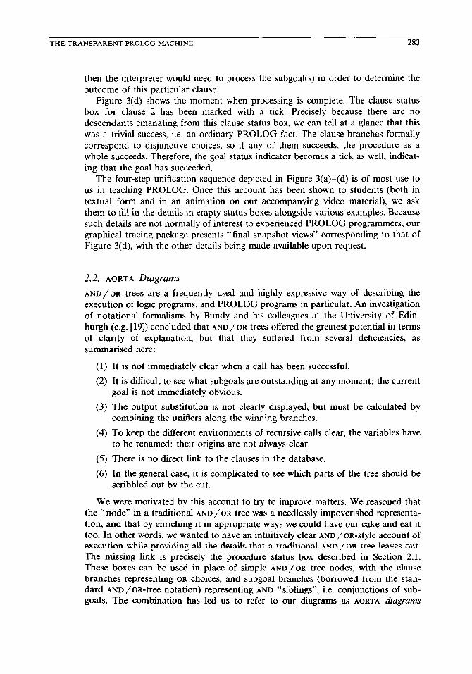
then the interpreter would need to process the subgoal(s) in order to determine the outcome of this particular clause.
Figure 3(d) shows the moment when processing is complete. The clause status box for clause 2 has been marked with a tick. Precisely because there are no descendants emanating from this clause status box, we can tell at a glance that this was a trivial success, i.e. an ordinary PROLOG fact. The clause branches formally correspond to disjunctive choices, so if any of them succeeds, the procedure as a whole succeeds. Therefore, the goal status indicator becomes a tick as well, indicat- ing that the goal has succeeded.
The four-step unification sequence depicted in Figure 3(a)-(d) is of most use to us in teaching PROLOG. Once this account has been shown to students (both in textual form and in an animation on our accompanying video material), we ask them to fill in the details in empty status boxes alongside various examples. Because such details are not normally of interest to experienced PROLOG programmers, our graphical tracing package presents “final snapshot views” corresponding to that of
Figure 3(d), with the other details being made available upon request.
2.2. AORTA Diagrams
AND/OR trees are a frequently used and highly expressive way of describing the execution of logic programs, and PROLOG programs in particular. An investigation of notational formalisms by Bundy and his colleagues at the University of Edin- burgh (e.g. [19]) concluded that AND/OR trees offered the greatest potential in terms of clarity of explanation, but that they suffered from several deficiencies, as summarised here:
(1) (2)
(3)
(4)
(5)
(6)
It is not immediately clear when a call has been successful.
It is difficult to see what subgoals are outstanding at any moment: the current goal is not immediately obvious.
The output substitution is not clearly displayed, but must be calculated by combining the unifiers along the winning branches.
To keep the different environments of recursive calls clear, the variables have to be renamed: their origins are not always clear.
There is no direct link to the clauses in the database.
In the general case, it is complicated to see which parts of the tree should be scribbled out by the cut.
We were motivated by this account to try to improve matters. We reasoned that the “node” in a traditional AND/OR tree was a needlessly impoverished representa- tion, and that by enriching it in appropriate ways we could have our cake and eat it too. In other words, we wanted to have an intuitively clear AND/OR-Style account of execution while providing all the details that a traditional AND/OR tree leaves out.
The missing link is precisely the procedure status box described in Section 2.1. These boxes can be used in place of simple AND/OR tree nodes, with the clause branches representing OR choices, and subgoal branches (borrowed from the stan- dard AND/OR-tree notation) representing AND “siblings", i.e. conjunctions of sub-
goals. The combination has led us to refer to our diagrams as AORTA diagrams
284 MARCEISENSTADTANDMIKEBRAYSHAW
fun(X) :- red(X), car(X). fun(X) :- blue(X), bike(X).
red(apple_ 1). red(block_ 1). red(car_27).
car(desoto_48). car(edsel_57).
blue(flower_3). blue(glass_9). blue(honda_81).
bike&is_8). bike(my_bike). bike(honda_81).
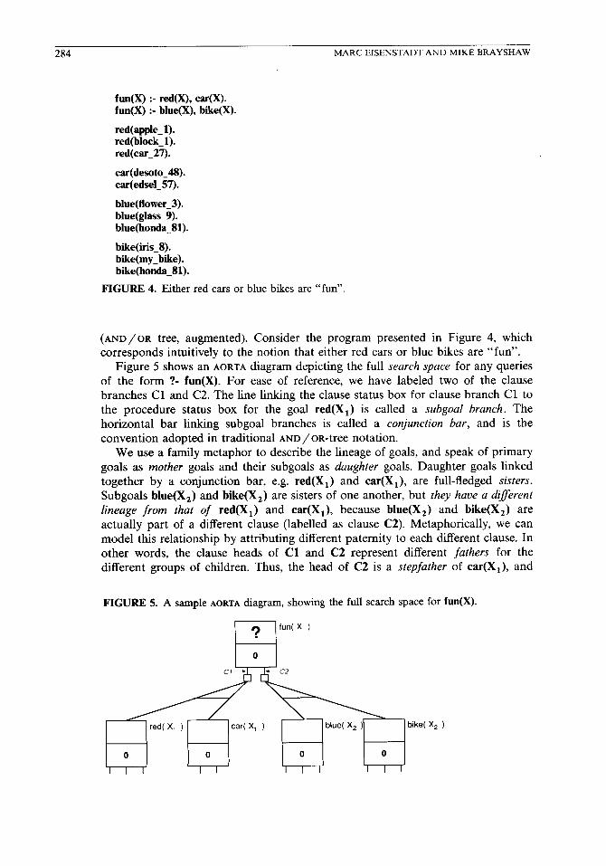
FIGURE 4. Ether red cars or blue bikes are “fun”.
(AND/OR tree, augmented). Consider the program presented in Figure 4, which corresponds intuitively to the notion that either red cars or blue bikes are “fun”.
Figure 5 shows an AORTA diagram depicting the full search space for any queries of the form ?- fun(X). For ease of reference, we have labeled two of the clause branches Cl and C2. The line linking the clause status box for clause branch Cl to the procedure status box for the goal red(X,) is called a subgoal brunch. The horizontal bar linking subgoal branches is called a conjunction bar, and is the convention adopted in traditional ~~~/o~-tree notation.
We use a family metaphor to describe the lineage of goals, and speak of primary goals as mother goals and their subgoals as daughter goals. Daughter goals linked together by a conjunction bar, e.g. red(X,) and car(X,), are full-fledged sisters. Subgoals blue&) and bike(X,) are sisters of one another, but they have a diflerent lineage from that of red(X,) and car(X,), because blue(X,) and bike(X,) are actually part of a different clause (labelled as clause C2). Metaphorically, we can model this relationship by attributing different paternity to each different clause. In other words, the clause heads of Cl and C2 represent different fathers for the different groups of children. Thus, the head of C2 is a stepfather of car(X,), and
FIGURE 5. A sample AORTA diagram, showing the full search space for fun(X).
? fun( x )
0
W X, ) cart X, ) blue( X, ) bike(
0 0 0 0
I I I I I I I I I I I.
x2 )
THETRANSPARENTPROLOGMACHINE 285
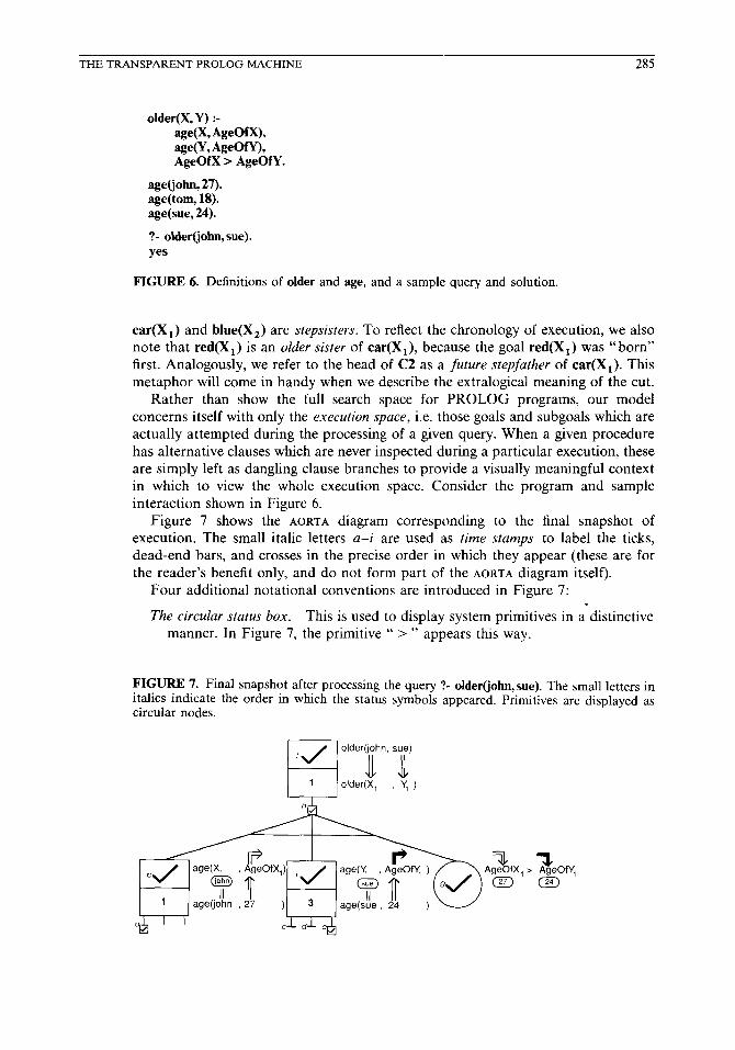
older@, Y) :- ape& Agem, age(Y, AgeOf% AgeOfX > AgeOfY.
age(john, 27). age(tom, 18). age(sue, 24).
?- older(john, sue).
yes
FIGURE 6. Definitions of older and age, and a sample query and solution.
car(X,) and blue(X,) are stepsisters. To reflect the chronology of execution, we also note that red(X,) is an older sister of car(X,), because the goal red(X,) was “born” first. Analogously, we refer to the head of C2 as a future stepfather of car(X,). This
metaphor will come in handy when we describe the extralogical meaning of the cut. Rather than show the full search space for PROLOG programs, our model
concerns itself with only the execution space, i.e. those goals and subgoals which are actually attempted during the processing of a given query. When a given procedure has alternative clauses which are never inspected during a particular execution, these are simply left as dangling clause branches to provide a visually meaningful context in which to view the whole execution space. Consider the program and sample interaction shown in Figure 6.
Figure 7 shows the AORTA diagram corresponding to the final snapshot of execution. The small italic letters a-i are used as time stumps to label the ticks, dead-end bars, and crosses in the precise order in which they appear (these are for the reader’s benefit only, and do not form part of the AORTA diagram itself).
Four additional notational conventions are introduced in Figure 7: .
The circular status box. This is used to display system primitives in a distinctive manner. In Figure 7, the primitive “ > ” appears this way.
FIGURE 7. Final snapshot after processing the query ?- older(john, sue). The small letters in italics indicate the order in which the status symbols appeared. Primitives are displayed as circular nodes.
286 MARCEISENSTADTANDMIKEBIUYSHAW
Right-angle arrows. When a variable appears more than once in a given clause, a right-angle arrow can be used to show how its instantiation is “passed across” from one occurrence to another. In Figure 7, we see that AgeOfX, is an output variable where it first appears in the goal age(X,, AgeOfX,), and that it becomes instantiated to 27 (just before timestamp a, in fact). In its second appearance, AgeOfX, is already instantiated by the time the subgoal AgeOfX,>AgeOfY, is processed (timestamp g), and notice that the right-angle arrow shows it correctly as an input variable at this point. The variable AgeOfY, is handled analogously, and shading is used just to keep the matching pairs of arrows visually distinct.
Lozenges. In an AORTA diagram, every variable in principle has a little lozenge underneath it which shows the variable’s current instantiation. In practice, we adopt a “tidying” convention which allows us to omit a lozenge whenever there is a straight up arrow or down arrow that lets us see the actual instantiation at a glance. We have found that the lozenges are absolutely vital for showing the details of unification, but that without the tidying convention the diagrams become needlessly cluttered. In effect, the appearance of a lozenge means that a given instantiation has come “from elsewhere”. We deliberately avoid the inclusion of linking arrows depicting exactly what “from elsewhere” means, because such arrows not only become unwieldy in complex diagrams, but are actually redundant. The reader may wish to confirm that the lozenge underneath the X, in the lower left-hand part of Figure 7 can only mean that X, was an input variable in that situation, and therefore a down arrow above that X, is unnecessary.
Headless arrows. This is actually a sideways “ = “, direct match between two terms. This can also uninstantiated variables share.
which conveniently shows a be used to show when two
Because it is inherently difficult to capture the dynamic nature of AORTA
diagrams in a static medium such as printed text, the reader may find it useful to
work through timestamps a-i of Figure 7, and to confirm the following two
observations: (1) the lozenges containing john and 27 are filled (i.e., the variables Xi and AgeOfX, are instantiated) just before the tick labeled with timestamp a appears; (2) the lozenges containing sue and 24 are filled (i.e., the variables Y, and AgeOfY, are instantiated) just between timestamps d and e. In our textual presen- tation of AORTA diagrams [12], we include numerous execution snapshot sequences, with unfilled lozenges left for our students to fill in. The replay facility of our graphical tracer (as well as the video animation sequences used in our course materials) allows us to show the dynamics of program execution in a more suitable manner.
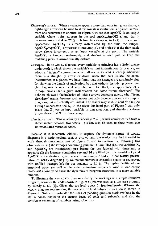
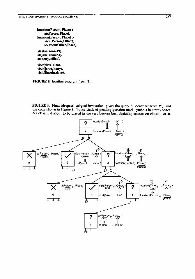
To illustrate the way AORTA diagrams clarify the workings of a simple recursive program, consider the code shown in Figure 8 (this was used as a test-case program by Bundy et al., [l]). Given the top-level query ?- location(lincoln, Where), the AORTA diagram representing the moment of final subgoal invocation is shown in Figure 9. Notice in particular the stack of pending question-mark symbols in the status boxes, depicting the current focus of goals and subgoals, and also the consistent renaming of variables using subscripts.
THE TRANSPARENT PROLOG MACHINE 287
location(Person, Place) :- at(Pemn, Place).
hation(Perso~ Place) :- visit(Person, Other), location(Other, Place).
at(alan, rooml9). at(jane, room54). at(betty, office).
visit(dave, alan). visit(janet, bet@). visit(lincoln, dave).
FIGURE 8. location program from [l].
FIGURE 9. Final (deepest) subgoal invocation, given the query ?- location(lincoln, W), and the code shown in Figure 8. Notice stack of pending question-mark symbols in status boxes. A tick is just about to be placed in the very bottom box, depicting success on clause 1 of at.
~~location(lincoln , W )
IT Place, )
l-t Place, ) @ig
288 MARCEISENSTADTANDMIKEBRAYSHAW
At the moment of the snapshot in Figure 9, a tick is just about to be placed in the very bottom box, indicating a trivial success (fact) on clause 1 of at. Remember from our discussion of Figure 3(c) that unification of a goal with a clause head precedes the processing of the clause body, even when that body contains a trivially true subgoal, i.e. when it is an ordinary PROLOG fact. As Figure 9 shows, Place, is instantiated to room19 at the bottom of the diagram. The lozenges and unification arrows reveal that Place,, Place,, and W are also instantiated to room 19, in effect at the same time as Place, is so instantiated. If we were to show the remaining eight execution snapshots, we would see a succession of tick symbols “bubbling up” to the top one snapshot at a time, but it is significant that the instantiation of W has taken place eight snapshots before the final success.
Let’s now reconsider the first five disadvantages of AND/OR tree representations raised by Pain and Bundy (and the way AORTA diagram notation overcomes these
disadvantages):
“It is not immediately clear when a call has been successful.” (This is instantly clear in the AORTA diagram when a question-mark symbol turns into a tick.)
“It is difficult to see what subgoals are outstanding at any moment: the current goal is not immediately obvious.” (The question-mark symbols in the AORTA
diagrams make this obvious.)
“The output substitution is not clearly displayed, but must be calculated by combining the unifiers along the winning branches.” [The unification arrows and lozenges show variable instantiation unambiguously; even more painstak- ing detail can be revealed upon request, as shown in Figure 3(a)-(d).]
“To keep the different environments of recursive calls clear, the variables have to be renamed: their origins are not always clear.” (AORTA diagrams use sub- scripting of user-provided variable names, so that the origins are completely clear. The objection implied by the use of the words “have to” is that it is difficult or confusing to perform renaming; we find that renaming is not actually difficult in practice, and moreover that renaming is essential to conform to the “true story” of PROLOG execution.)
“There is no direct link to the clauses in the database.” (The AORTA status-box clause counter provides precisely such a link, assuming of course that the user bothers to obtain a code listing or display the code in a separate window on
the screen.)
The sixth disadvantage (display of cut details) is dealt with in Section 2.5. We believe that the AORTA diagrams incorporate all of the best features of AND/OR
trees, and overcome all of their disadvantages. More complicated cases involving unification of large terms, reinvocation of goals after backtracking, and the cut are shown in the following sections.
2.3. Compound-Term Unification and Large Databases
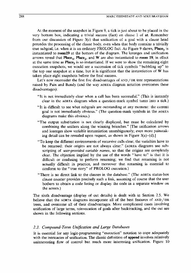
It is essential for any logic-progr amming “execution” notation to cope adequately with the intricacies of unification. The classic definition of append involves relatively uninteresting flow of control but much more interesting unification. Figure 10
THETRANSPARENTPROLOGMACHINE 289
append(l I, Ys, Ys).
append([X I W,Ys, Ix I Zsl) :- append(Xs, Ys, Zs).
?- append([a, b], [c, d], What). What = [a, b, c, d]
FIGURE 10. Classic definition of append, and a sample query and solution.
presents both the definition and a sample query. Figure 11 shows the AORTA
execution snapshot at the moment this query has succeeded. There are three subtleties to note about Figure 11:
Lists are expanded to show the head and tail explicitly just in those places where
A
_ _ it is critical to reveal the precise correspondence for unification purposes. For instance, the first argument of the top level goal is displayed as [a 1 [b] ] rather than [a,b], thereby making the instantiations of X, and Xs, obvious at a glance. Notice that the lozenge underneath the variable What similarly shows the head and tail corresponding to the instantiations of X, and Zs,. The lozenge beneath the topmost appearance of Zs, shows the list [b,c,d] in its “beautified” form, because a deeper account of the internal structure is not necessary there. However, where Zs, appears near the middle of the diagram, a deeper account of the internal structure is necessary to show the instantia- tions of X, and Zs,, so the lozenge is shown containing the list [b 1 [c, d] 1.
thin horizontal line is drawn at the base of unification arrows to encompass entire compound terms (structures), thereby showing that it is the whole term (rather than a single atom within it) which has been unified. For instance, where Ys, is instantiated to [c,d] at the top of Figure 5, the line at the base of
d
%
append([ a I [bl lkdl, WI&t ) yJ pyai)
2 aweWX,l %I. Ys, 3 IX,1 Zs, 1)
FIGURE 11. AORTA diagram corresponding of the query ?- append([a, b], [c, d], What).
to solution
290 MARC EISENSTADT AND MIKE BRAYSHAW
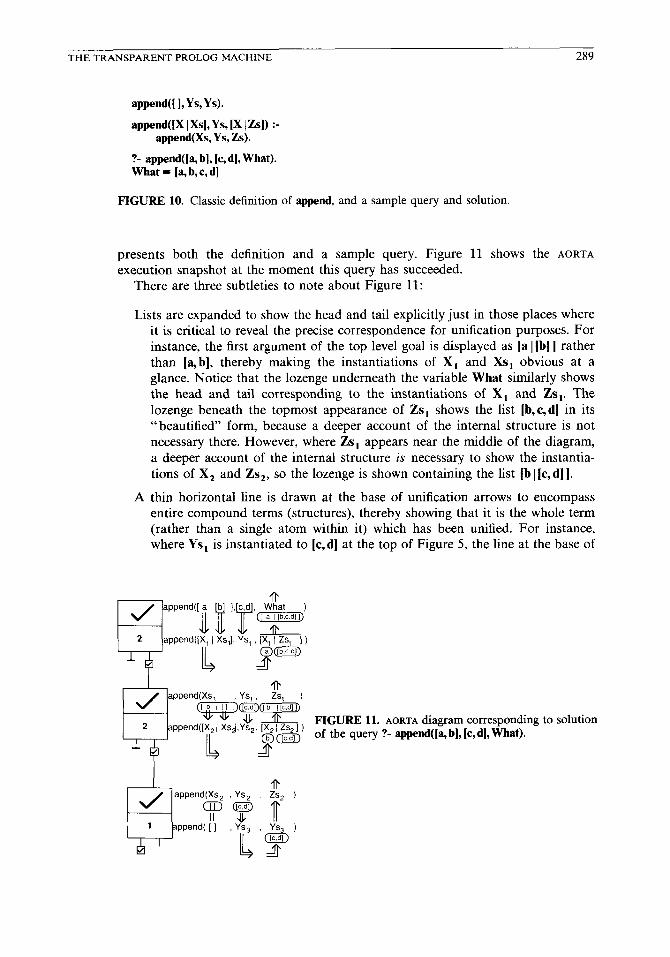
london, new-York, Dep, ,Arr, , Days, ) FIGURE 12. Procedure status box used
london, new-York, 1000 ,1400,[m,t,w,th,f]) for large databases.
the relevant arrow tells us that it is the entire term [c,d] which is involved, rather than just the atom c.
When an arrow points down from below (or up towards) a lozenge as a whole, then the full content of that lozenge is involved. On the other hand, when part of the arrow crosses the border of a lozenge, then only the particular term being pointed from (or to) is involved. Consider, for example, the procedure status box in the middle of Figure 11. The arrow pointing to Ys, emanates from below the lozenge containing [c,d], and thus the entire term [c,d] is involved. However, the arrow pointing down to X, crosses the border of a lozenge, meaning that only the term b is involved. The term b happens to be an atom, but in general a compound term might be involved, in which case a horizontal line would be used at the base of the unification arrow to show the extent of the term.
While compound terms can in general be dealt with in the manner described above, the sheer size of certain terms in real PROLOG programs necessitates the use of special collapsing conventions. We use hand-crafted (i.e. carefully positioned) ellipsis dots (,‘ . . . “) in our textual displays when appropriate, and a special small font in our graphical tracer implementation to show the unification of very large terms. We also allow the user of our graphical tracer to specify an ellipsis template for the display of large terms, which works much like PROLOG’s portray primitive (except that it is accomplished with a pop-up dialogue box).
Large terms are not the only practical problem we have to face: large databases may contain hundreds (or even thousands) of clauses in the definition of a given procedure. To cater for this, we adopt a collapsing convention in the procedure status box. In Figure 12, we show a hypothetical example of a goal used to access a large database of airline flights containing 429 clauses of the predicate flight. Rather than showing all clause branches, we only show the ones whose heads actually unified with the goal2 The small numbers above each clause branch indicate precisely which clauses were involved (in the example shown, only clauses 7, 59,121, 147, and 231 had heads which unified with the goal). All the ones which are omitted would, had there been enough room, have been displayed as dead-end bars, because the omitted ones are precisely those whose heads did not unify with the goal. The large 429 in Figure 12 means that this particular procedure had 429 clauses altogether. The 231 in the horizontal scroll box is the actual clause counter, indicating that clause 231 is the one under consideration at the moment this
2The past tense is deliberate here. Our implementation normally does a “post-mortem” analysis, so we know exactly which clause heads unified and which didn’t. It is also possible to run the system in live-trace mode, as described in Section 3.
THETRANSPARENTPROLOGMACHINE 291
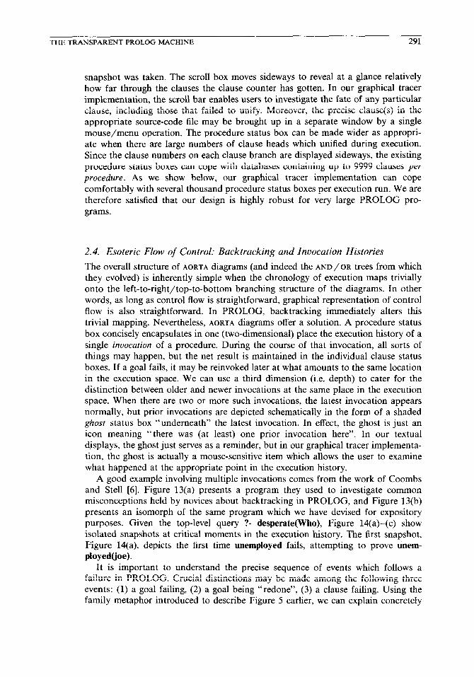
snapshot was taken. The scroll box moves sideways to reveal at a glance relatively how far through the clauses the clause counter has gotten. In our graphical tracer implementation, the scroll bar enables users to investigate the fate of any particular clause, including those that failed to unify. Moreover, the precise clause(s) in the appropriate source-code file may be brought up in a separate window by a single mouse/menu operation. The procedure status box can be made wider as appropri- ate when there are large numbers of clause heads which unified during execution. Since the clause numbers on each clause branch are displayed sideways, the existing procedure status boxes can cope with databases containing up to 9999 clauses per procedure. As we show below, our graphical tracer implementation can cope comfortably with several thousand procedure status boxes per execution run. We are therefore satisfied that our design is highly robust for very large PROLOG pro- grams.
2.4. Esoteric Flow of Control: Backtracking and Invocation Histories
The overall structure of AORTA diagrams (and indeed the AND/OR trees from which they evolved) is inherently simple when the chronology of execution maps trivially onto the left-to-right/top-to-bottom branching structure of the diagrams. In other words, as long as control flow is straightforward, graphical representation of control flow is also straightforward. In PROLOG, backtracking immediately alters this trivial mapping. Nevertheless, AORTA diagrams offer a solution. A procedure status
box concisely encapsulates in one (two-dimensional) place the execution history of a single invocation of a procedure. During the course of that invocation, all sorts of things may happen, but the net result is maintained in the individual clause status boxes. If a goal fails, it may be reinvoked later at what amounts to the same location in the execution space. We can use a third dimension (i.e. depth) to cater for the distinction between older and newer invocations at the same place in the execution space. When there are two or more such invocations, the latest invocation appears normally, but prior invocations are depicted schematically in the form of a shaded ghost status box “underneath” the latest invocation. In effect, the ghost is just an icon meaning “there was (at least) one prior invocation here”. In our textual displays, the ghost just serves as a reminder, but in our graphical tracer implementa- tion, the ghost is actually a mouse-sensitive item which allows the user to examine what happened at the appropriate point in the execution history.
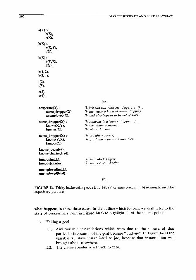
A good example involving multiple invocations comes from the work of Coombs and Stell [6]. Figure 13(a) presents a program they used to investigate common misconceptions held by novices about backtracking in PROLOG, and Figure 13(b) presents an isomorph of the same program which we have devised for expository purposes. Given the top-level query ?- desperate(Who), Figure 14(a)-(c) show isolated snapshots at critical moments in the execution history. The first snapshot, Figure 14(a), depicts the first time unemployed fails, attempting to prove unem- ployed(joe).
It is important to understand the precise sequence of events which follows a failure in PROLOG. Crucial distinctions may be made among the following three events: (1) a goal failing, (2) a goal being “redone”, (3) a clause failing. Using the family metaphor introduced to describe Figure 5 earlier, we can explain concretely
292 MARC EISENSTADT AND MIKE BRAYSHAW
a(X) :- b0, c(x).
b(X) :- h(X, Y), i(Y).
b(X) :- h(Y, x), i(Y).
h(l, 2). h(3,4).
i(2). i(3).
c(2). c(4).
desperate(X) :- name_dropper(X), unemployed(X).
name-dropper(X) :- knows(x, Y), famous(Y).
name-dropper(X) :- knows(Y, x), famous(Y).
knows(joe, mick). knows(charles, fred).
famous(mick). famous(charles).
unemployed(mick). unemployed(fred).
% We can call someone ‘desperate ’ if. . 4% they have a habit of name-dropping 4% and also happen to be out of work.
% someone is a ‘name_dropper ’ if. . % they know someone.. % who is famous
% or, alternatively, % if a famous person knows them
5% say, Mick Jagger % say, Prince Charies
FIGURE 13. Tricky backtracking code from [6]: (a) original program; (b) isomorph, used for expository purposes.
what happens in these three cases. In the outline which follows, we shall refer to the state of processing shown in Figure 14(a) to highlight all of the salient points:
1. Failing a goal
1.1. Any variable instantiations which were due to the success of that particular invocation of the goal become “undone”. In Figure 14(a) the variable Xi stays instantiated to joe, because that instantiation was brought about elsewhere.
1.2. The clause counter is set back to zero.

THE TRANSPARENT PROLOG MACHINE 293
knows(joe , mick )
name_dropper(X, )
name_dropper(X, )
knows(Y, , X, )
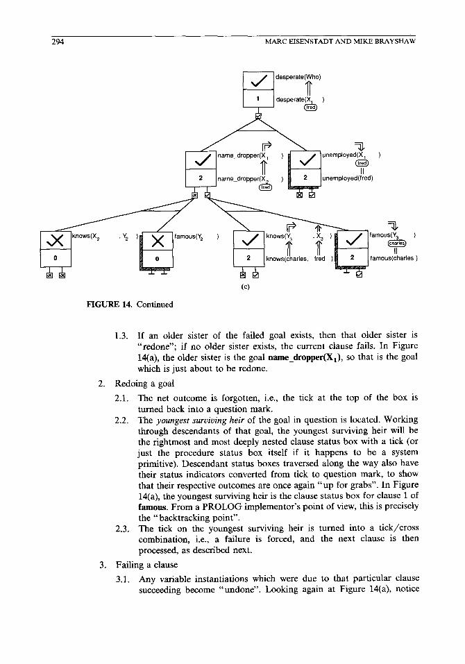
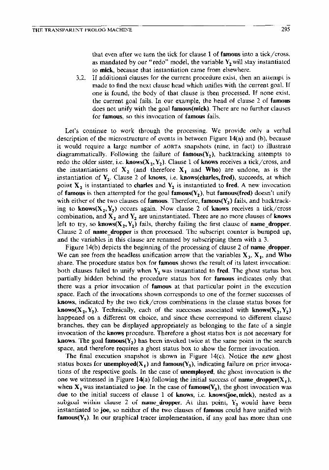
given code shown in FIGURE 14. Execution snapshot following query ?- desperate(Who), Figure 13(b): (a) The moment of first failure of unemployed. (b) Just about to attempt second clause of name_dropper. Notice that name-dropper is the current focus, and that famous had a prior invocatron which succeeded but then failed on backtracking. The current invocation of famous merely failed because no clause heads matched. (c) Final snapshot. Both famous and unemployed failed on prior invocations.
294 MARC EISENSTADT AND MIKE BRAYSHAW
knows(c!harles, f&d )
Cc)
FIGURE 14. Continued
1.3. If an older sister of the failed goal exists, then that older sister is
“ redone”; if no older sister exists, the current clause fails. In Figure 14(a), the older sister is the goal name_dropper(X,), so that is the goal
which is just about to be redone.
2. Redoing a goal
2.1.
2.2.
2.3.
The net outcome is forgotten, i.e., the tick at the top of the box is turned back into a question mark. The youngest suruiuing heir of the goal in question is located. Working through descendants of that goal, the youngest surviving heir will be the rightmost and most deeply nested clause status box with a tick (or just the procedure status box itself if it happens to be a system primitive). Descendant status boxes traversed along the way also have their status indicators converted from tick to question mark, to show that their respective outcomes are once again “up for grabs”. In Figure 14(a), the youngest surviving heir is the clause status box for clause 1 of famous. From a PROLOG implementor’s point of view, this is precisely the “backtracking point”. The tick on the youngest surviving heir is turned into a tick/cross combination, i.e., a failure is forced, and the next clause is then processed, as described next.
3. Failing a clause
3.1. Any variable instantiations which were due to that particular clause succeeding become “undone”. Looking again at Figure 14(a), notice
THETRANSPARENTPROLOGMACHINE 295
3.2.
that even after we turn the tick for clause 1 of famous into a tick/cross, as mandated by our “redo” model, the variable Y2 will stay instantiated
to mick, because that instantiation came from elsewhere. If additional clauses for the current procedure exist, then an attempt is made to find the next clause head which unifies with the current goal. If one is found, the body of that clause is then processed. If none exist, the current goal fails. In our example, the head of clause 2 of famous does not unify with the goal famous(mick). There are no further clauses for famous, so this invocation of famous fails.
Let’s continue to work through the processing. We provide only a verbal description of the microstructure of events in between Figure 14(a) and (b), because it would require a large number of AORTA snapshots (nine, in fact) to illustrate diagrammatically. Following the failure of famous&), backtracking attempts to redo the older sister, i.e. knows(X,,Y,). Clause 1 of knows receives a tick/cross, and the instantiations of X, (and therefore X, and Who) are undone, as is the instantiation of Yz. Clause 2 of knows, i.e. knows(charles,fred), succeeds, at which point X, is instantiated to Charles and Y2 is instantiated to fred. A new invocation of famous is then attempted for the goal famous(Y,), but famous(fred) doesn’t unify with either of the two clauses of famous. Therefore, famous(Y,) fails, and backtrack- ing to knows(X,,Y,) occurs again. Now clause 2 of knows receives a tick/cross combination, and X, and Yz are uninstantiated. There are no more clauses of knows left to try, so knows(X,,Y,) fails, thereby failing the first clause of name-dropper. Clause 2 of name dropper is then processed. The subscript counter is bumped up, and the variables in this clause are renamed by subscripting them with a 3.
Figure 14(b) depicts the beginning of the processing of clause 2 of name-dropper. We can see from the headless unification arrow that the variables X,, X,, and Who share. The procedure status box for famous shows the result of its latest invocation: both clauses failed to unify when Y2 was instantiated to fred. The ghost status box partially hidden behind the procedure status box for famous indicates only that there was a prior invocation of famous at that particular point in the execution
space. Each of the invocations shown corresponds to one of the former successes of knows, indicated by the two tick/cross combinations in the clause status boxes for knows(X,, Yz). Technically, each of the successes associated with knows(X,, Yz) happened on a different OR choice, and since these correspond to different clause branches, they can be displayed appropriately as belonging to the fate of a single invocation of the knows procedure. Therefore a ghost status box is not necessary for knows. The goal famous&) has been invoked twice at the same point in the search space, and therefore requires a ghost status box to show the former invocation.
The final execution snapshot is shown in Figure 14(c). Notice the new ghost status boxes for unemployed(X,) and famous(k;), indicating failure on prior invoca- tions of the respective goals. In the case of unemployed, the ghost invocation is the one we witnessed in Figure 14(a) following the initial success of name_dropper(X,), when X, was instantiated to joe. In the case of famous&), the ghost invocation was due to the initial success of clause 1 of knows, i.e. knows(joe,mick), nested as a subgoal within clause 2 of name-dropper. At that point, Y3 would have been instantiated to joe, so neither of the two clauses of famous could have unified with famous(Y& In our graphical tracer implementation, if any goal has more than one
296 MARCEISENSTADTANDMIKEBRAYSHAW
prior invocation (still indicated by a single ghost status box), it is possible for the user to step through them individually by mouse-clicking on the ghost. This rewinds the execution replay to the time point when the previous invocation occurred. The previous invocation may of course have its own ghost (i.e. an even earlier invoca- tion), which in turn will be selectable by the user. An alternative method is to reobserve the complete execution sequence from the beginning, using the fast-for- ward and single-step capabilities described in Section 3.
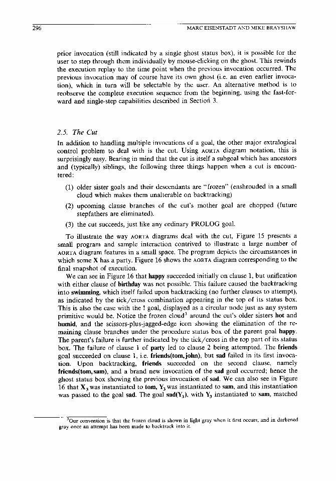
2.5. The Cut
In addition to handling multiple invocations of a goal, the other major extralogical control problem to deal with is the cut. Using AORTA diagram notation, this is surprisingly easy. Bearing in mind that the cut is itself a subgoal which has ancestors and (typically) siblings, the following three things happen when a cut is encoun- tered:
(1) older sister goals and their descendants are “frozen” (enshrouded in a small
cloud which makes them unalterable on backtracking)
(2) upcoming clause branches of the cut’s mother goal are chopped (future stepfathers are eliminated).
(3) the cut succeeds, just like any ordinary PROLOG goal.
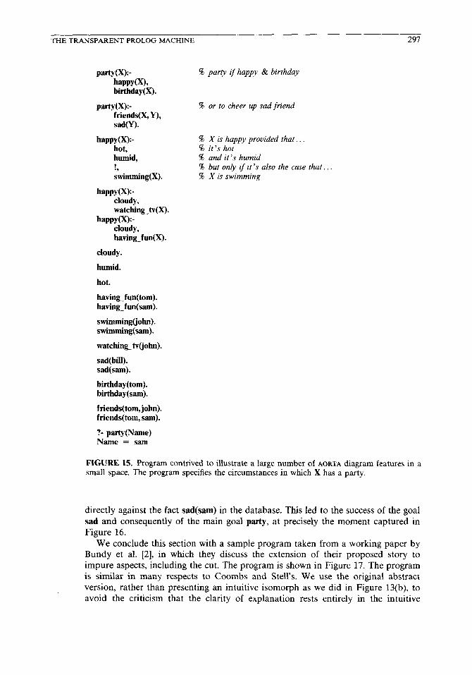
To illustrate the way AORTA diagrams deal with the cut, Figure 15 presents a small program and sample interaction contrived to illustrate a large number of AORTA diagram features in a small space. The program depicts the circumstances in which some X has a party. Figure 16 shows the AORTA diagram corresponding to the
final snapshot of execution. We can see in Figure 16 that happy succeeded initially on clause 1, but unification
with either clause of birthday was not possible. This failure caused the backtracking into swimming, which itself failed upon backtracking (no further clauses to attempt), as indicated by the tick/cross combination appearing in the top of its status box. This is also the case with the ! goal, displayed as a circular node just as any system primitive would be. Notice the frozen cloud3 around the cut’s older sisters hot and humid, and the scissors-plus-jagged-edge icon showing the elimination of the re- maining clause branches under the procedure status box of the parent goal happy. The parent’s failure is further indicated by the tick/cross in the top part of its status box. The failure of clause 1 of party led to clause 2 being attempted. The friends goal succeeded on clause 1, i.e. friends(tom,john), but sad failed in its first invoca- tion. Upon backtracking, friends succeeded on the second clause, namely friends(tom,sam), and a brand new invocation of the sad goal occurred; hence the ghost status box showing the previous invocation of sad. We can also see in Figure 16 that X, was instantiated to tom, Y3 was instantiated to sam, and this instantiation was passed to the goal sad. The goal sad(Y,), with Ys instantiated to sam, matched
‘Our convention is that the frozen cloud is shown in light gray when it first occurs, and in darkened gray once an attempt has been made to backtrack into it.
THE TRANSPARENT PROLOG MACHINE 297
Partyco- bw(W9 birthday(X).
PartyCQ- friends(X, Y), sad(Y).
haPPY(x):- hot, humid, I &mming(X).
hapPy(X):- cloudy, watching_tv(X).
happy(X):- cloudy, having-fun(X).
cloudy.
humid.
hot.
having_fun(tom). having_fun(sam).
swimming(john). swimming(sam).
watching_tv(john).
sad(bill). sad( Sam).
birthday(tom). birthday(sam).
friends(tom, john). friends(tom, sam).
?- party(Name) Name = sam
% party if happy & birthday
% or to cheer up sad friend
% X is happy provided that.. % it’s hot % and it’s humid % but only if it’s also the case that. . % X is swimming
FIGURE 15. Program contrived to illustrate a large number of AORTA diagram features in a small space. The program specifies the circumstances in which X has a party.
directly against the fact sad(sam) in the database. This led to the success of the goal sad and consequently of the main goal party, at precisely the moment captured in Figure 16.
We conclude this section with a sample program taken from a working paper by Bundy et al. [2], in which they discuss the extension of their proposed story to impure aspects, including the cut. The program is shown in Figure 17. The program is similar in many respects to Coombs and Stell’s. We use the original abstract version, rather than presenting an intuitive isomorph as we did in Figure 13(b), to avoid the criticism that the clarity of explanation rests entirely in the intuitive
298 MARCEISENSTADTANDMIKEBRAYSHAW
IhawW, )I v Ibifihdayo(, ) I
x
i,
0
swimming
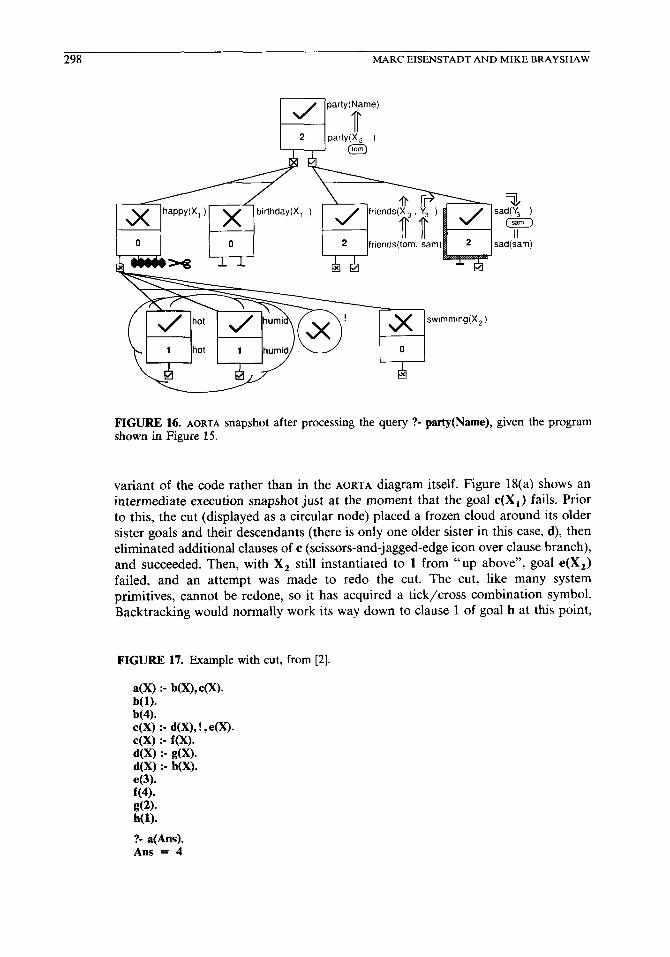
FIGURE 16. AORTA snapshot after processing the query ?- parly(Name), given the program shown in Figure 15.
variant of the code rather than in the AORTA diagram itself. Figure 18(a) shows an intermediate execution snapshot just at the moment that the goal c(X,) fails. Prior to this, the cut (displayed as a circular node) placed a frozen cloud around its older sister goals and their descendants (there is only one older sister in this case, d), then eliminated additional clauses of c (scissors-and-jagged-edge icon over clause branch), and succeeded. Then, with X, still instantiated to 1 from “up above”, goal e(X,) failed, and an attempt was made to redo the cut. The cut, like many system primitives, cannot be redone, so it has acquired a tick/cross combination symbol. Backtracking would normally work its way down to clause 1 of goal h at this point,
FIGURE 17. Example with cut, from [2].
a(X) :- b(X),@0 b(l). b(4). d2 :- f&l, !, e(X).
:- d(x) :- @i d(X) :- h(X). 43). f(4). g(2). h(l).
?- a(Ans). Ans = 4
THE TRANSPARENT PROLOG MACHINE 299
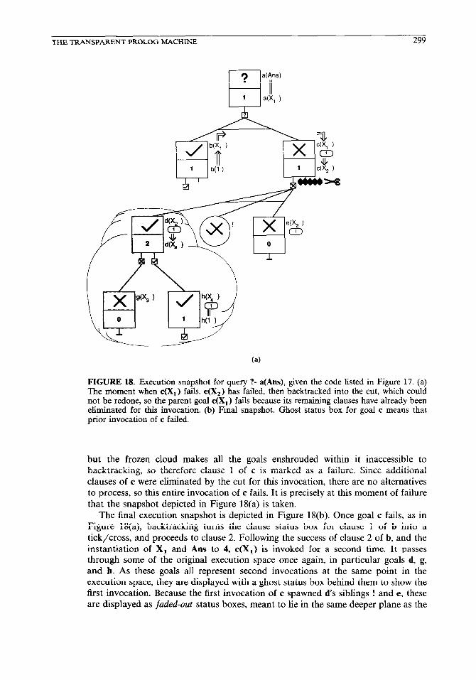
FIGURE 18. Execution snapshot for query ?- a(Ans), given the code listed in Figure 17. (a) The moment when c(X,) fails. e(X,) has failed, then backtracked into the cut, which could not be redone, so the parent goal c(X,) fails because its remaining clauses have already been eliminated for this invocation. (b) Final snapshot. Ghost status box for goal c means that prior invocation of c failed.
but the frozen cloud makes all the goals enshrouded within it inaccessible to backtracking, so therefore clause 1 of c is marked as a failure. Since additional clauses of c were eliminated by the cut for this invocation, there are no alternatives to process, so this entire invocation of c fails. It is precisely at this moment of failure that the snapshot depicted in Figure 18(a) is taken.
The final execution snapshot is depicted in Figure 18(b). Once goal c fails, as in Figure 18(a), backtracking turns the clause status box for clause 1 of b into a tick/cross, and proceeds to clause 2. Following the success of clause 2 of b, and the instantiation of X, and Am to 4, c(X,) is invoked for a second time. It passes through some of the original execution space once again, in particular goals d, g, and h. As these goals all represent second invocations at the same point in the execution space, they are displayed with a ghost status box behind them to show the first invocation. Because the first invocation of c spawned d’s siblings ! and e, these are displayed as faded-out status boxes, meant to lie in the same deeper plane as the
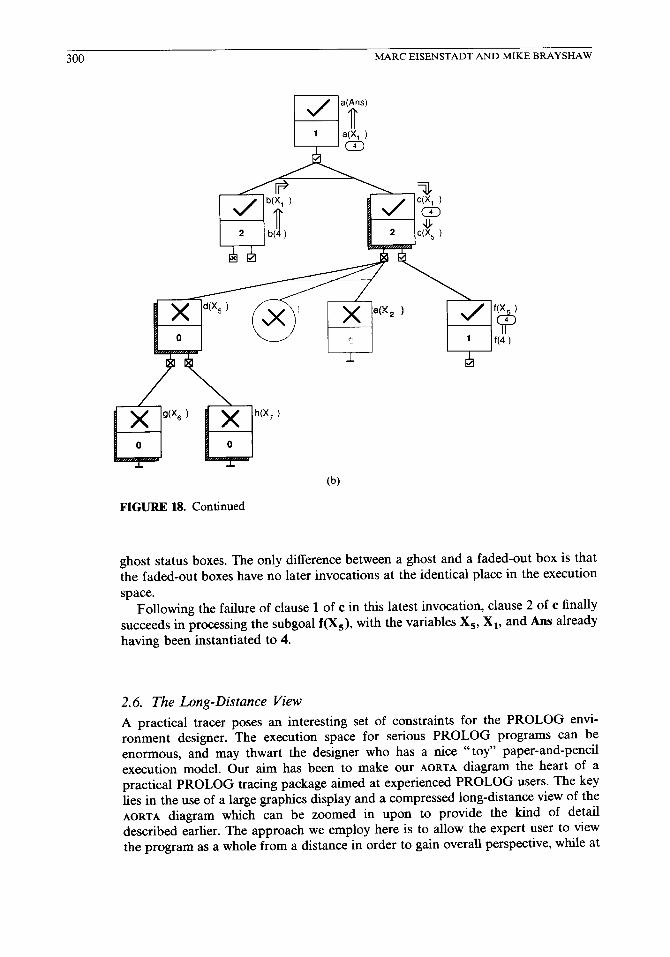
300 MARCEISENSTADTANDMIKEBRAYSHAW
/ g(X, ) ---I K W, )
(b)
FIGURE 18. Continued
ghost status boxes. The only difference between a ghost and a faded-out box is that the faded-out boxes have no later invocations at the identical place in the execution space.
Following the failure of clause 1 of c in this latest invocation, clause 2 of c finally
succeeds in processing the subgoal f(X,), with the variables X,, X,, and Ans already having been instantiated to 4.
2.6. The Long-Distance View
A practical tracer poses an interesting set of constraints for the PROLOG envi- ronment designer. The execution space for serious PROLOG programs can be enormous, and may thwart the designer who has a nice “toy” paper-and-pencil execution model. Our aim has been to make our AORTA diagram the heart of a practical PROLOG tracing package aimed at experienced PROLOG users. The key lies in the use of a large graphics display and a compressed long-distance view of the AORTA diagram which can be zoomed in upon to provide the kind of detail described earlier. The approach we employ here is to allow the expert user to view the program as a whole from a distance in order to gain overall perspective, while at
THETRANSPARENTPROLOGMACHINE 301
pending successful goal goal
LDV (user-defined q relation)
0
LDV (system 0 0 primitive)
LDV (compressed A user code)
n
falled succeeded, then
failed on goal backtracking
II
0 0
A n
prior invocation(s) at this place
la
e
A
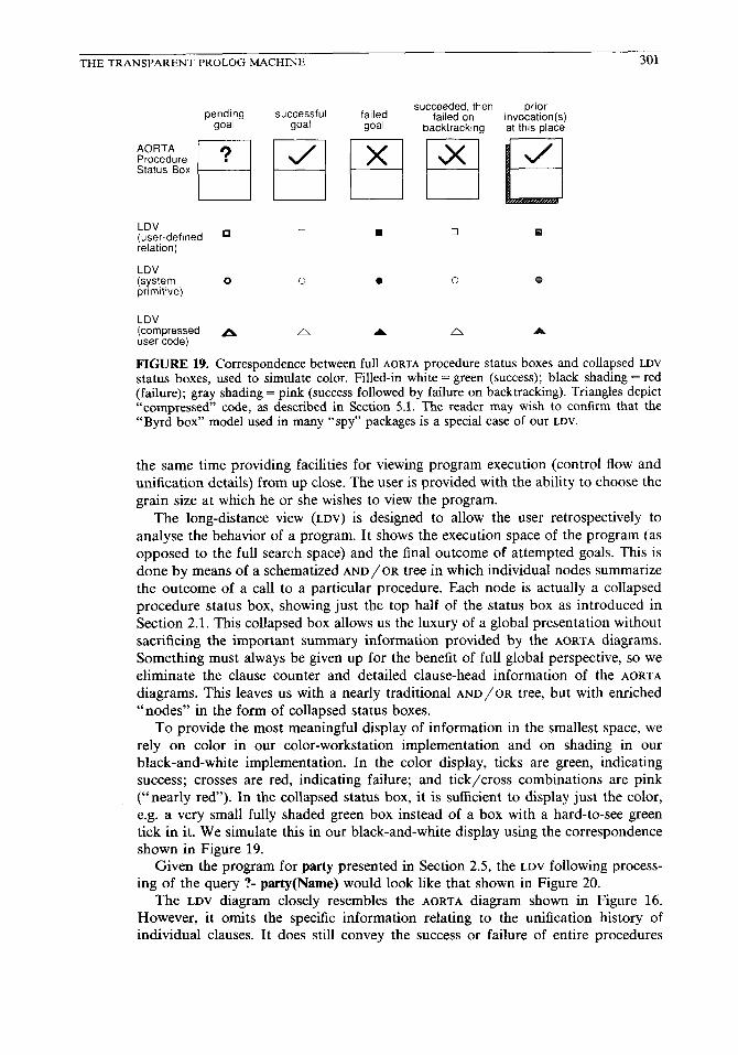
FIGURE 19. Correspondence between full AORTA procedure status boxes and collapsed LDV
status boxes, used to simulate color. Filled-in white = green (success); black shading = red (failure); gray shading = pink (success followed by failure on backtracking). Triangles depict “compressed” code, as described in Section 5.1. The reader may wish to confirm that the “Byrd box” model used in many “spy” packages is a special case of our LDV.
the same time providing facilities for viewing program execution (control flow and unification details) from up close. The user is provided with the ability to choose the
grain size at which he or she wishes to view the program. The long-distance view (LDV) is designed to allow the user retrospectively to
analyse the behavior of a program. It shows the execution space of the program (as opposed to the full search space) and the final outcome of attempted goals. This is done by means of a schematized AND/OR tree in which individual nodes summarize the outcome of a call to a particular procedure. Each node is actually a collapsed procedure status box, showing just the top half of the status box as introduced in Section 2.1. This collapsed box allows us the luxury of a global presentation without sacrificing the important summary information provided by the AORTA diagrams. Something must always be given up for the benefit of full global perspective, so we eliminate the clause counter and detailed clause-head information of the AORTA
diagrams. This leaves us with a nearly traditional AND/OR tree, but with enriched “nodes” in the form of collapsed status boxes.
To provide the most meaningful display of information in the smallest space, we rely on color in our color-workstation implementation and on shading in our black-and-white implementation. In the color display, ticks are green, indicating success; crosses are red, indicating failure; and tick/cross combinations are pink (“nearly red”). In the collapsed status box, it is sufficient to display just the color, e.g. a very small fully shaded green box instead of a box with a hard-to-see green tick in it. We simulate this in our black-and-white display using the correspondence shown in Figure 19.
Given the program for party presented in Section 2.5, the LDV following process- ing of the query ?- party(Name) would look like that shown in Figure 20.
The LDV diagram closely resembles the AORTA diagram shown in Figure 16. However, it omits the specific information relating to the unification history of individual clauses. It does still convey the success or failure of entire procedures

302 MARC EISENSTADT AND MIKE BRAYSHAW
FIGURE 20. Long-distance view showing the execution of the query ?- party(Name). Compare with Figure 16 to see the difference between the LDV and AORTA views of program execution. Note that the frozen cloud over the cut’s older sisters is retained even in the LDV, and that a circular node to the right of a frozen cloud is always a cut.
and, more importantly, the success or failure of whole branches of the tree. The more fine-grained information is omitted specifically to allow the user to view the history of execution of an entire program, and to view it in perspective, seeing branches of success or failure and the existence and scope of backtracking. It thus provides the user with a global view of the program from which to direct subsequent debugging in a top-down manner. The method for achieving this and the interactive use of these tools are described in the following sections.
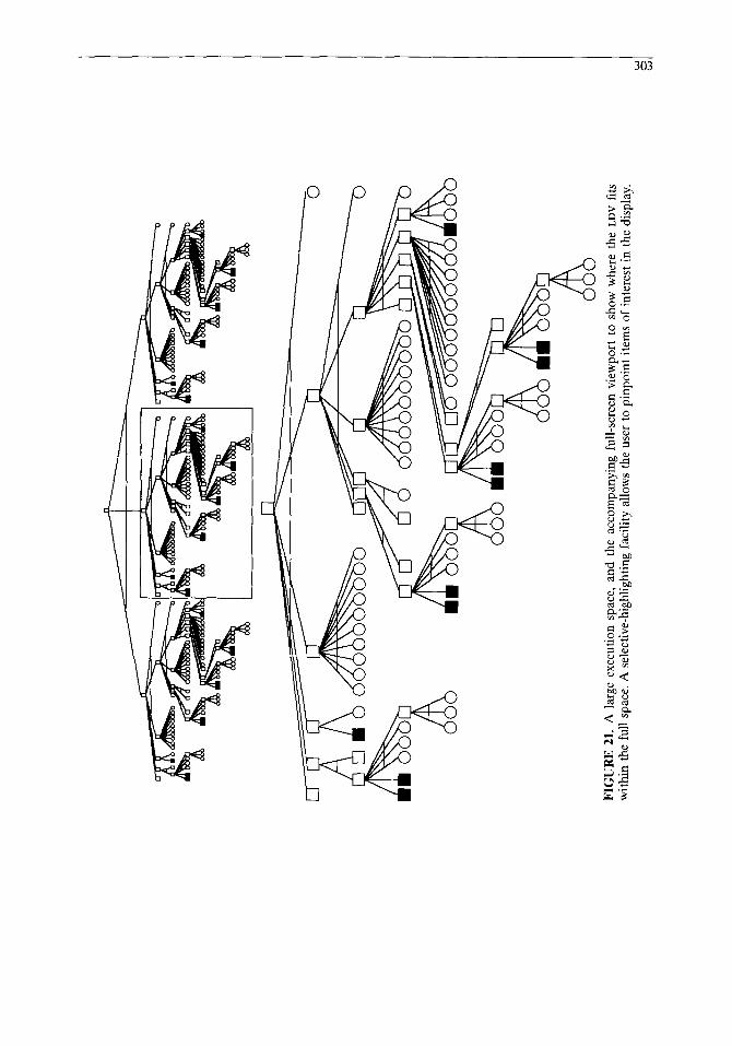
The succinct manner of the LDV representation also allows for the analysis of very large PROLOG programs. Even if the execution space is too large to be meaningfully displayed within a single graphics pane, the user is able to scroll around the pane, selecting the area of the tree which he or she wishes to look at. A facility to monitor which part of the tree is being observed ensures that the user maintains a global perspective on the whole tree. An example of a tree for a more realistic size of execution space is shown in Figure 21.
The execution space at the top of Figure 21 contains 310 nodes. Our current display can cope comfortably with 2500 nodes at the same resolution as that depicted in Figure 21. As an example of the powerful gestalt effects possible even in an unlabeled diagram, notice first the cluster of three circular nodes (depicting
primitive calls) at the deepest level of nesting of the tree. Now try to find the same pattern of three “circular sisters” elsewhere in the tree. Finally, put yourself in the
position of a programmer who has been developing the associated code over a period of days, and has become accustomed to the repetition of certain familiar shapes. Our point is that locating items of interest in the tree is surprisingly easy. Such items of interest can, of course, be inspected more closely, even while preserving a considerable amount of the surrounding context. In Section 3 we describe our selective highlighting facility which enables the programmer to high- light (by use of a characteristically eye-catching diamond surround) nodes in the tree which satisfy some particular constraint or behavioral description.
3. A WORKING TPM ENVIRONMENT
So far we have described the AORTA and LDV Views of the program trace. The following sections describe the way the user interacts with these descriptions, and other facilities and tools contained within the TPM environment. Our current implementation runs on 68020-based graphics workstations, and (except for some user-interface hooks) is written entirely in PROLOG.
FIG
UR
E
21.
A
larg
e ex
ecut
ion
spac
e,
and
the
acco
mpa
nyin
g fu
ll-sc
reen
vi
ewpo
rt
to
show
w
here
th
e L
DV
fi
ts
with
in
the
full
spac
e.
A s
elec
tive-
high
light
ing
faci
lity
allo
ws
the
user
to
pin
poin
t ite
ms
of i
nter
est
in
the
disp
lay.
304 MARCEISENSTADTANDMIKEBRAYSHAW
3.1. Initial Environment and Basic Facilities
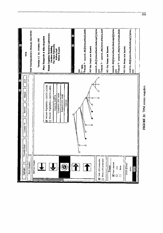
The interaction with the TPM environment is essentially via mouse and menu selection. A typical screen snapshot is shown in Figure 22. The resident interpreter/compiler is seen on the right, together with a transcript of the user’s interaction with it, in this instance in a window called Process_6. From this top level the graphical tracer is invoked by the query ?- tpm, which results in the appearance of the window we see on the left. The menu options, buttons, and mouse-sensitive graphics areas are described briefly below, after which the major facilities are treated in separate detail. In the summaries which follow, we start at the top left-hand corner of Figure 22 and initially work downwards.
Selective Highlight Button. This button produces a pop-up form, the purpose of which is to allow nodes in the LDV to be picked out by the user according to very specific features. For instance, the user can request the highlighting of all (and only) those calls to foo such that foo was a subgoal of bar and foo’s second argument was instantiated to, say, [a, b, c (Xl. Additionally the selected argument may have a series of constraints placed upon it. For example, we might ask for all occurrences of predicate count when its second argument is instantiated to some value which is greater than 10. It is also possible to apply a history filter, so that the user can highlight a specified goal at, say, precisely the moment before it failed for the first time, or just after its latest success.
Move Viewport. When the execution space is very large, as in Figure 21, the full-screen LDV only shows part of the whole space. The reduced view at the top of the screen shows the full space, and includes a moveable viewport which the user can select to be the full-screen viewing region.
Replay Control Panel. The user may choose to replay execution from some specific point in the execution history (or indeed from the very beginning), using the options in the control panel. The individual controls are, reading from the top, replay back to the beginning, single-step back, stop (this is highlighted in Figure 22) single-step forward, and ordinary forward. To the left of them is the replay speed bar, which changes the speed from slow to fast. Employing a video analogy, this allows the function of the forward button to be changed arbitrarily from “creep” through “play” to “fast forward”. The user can also move rapidly around the trace history by using the selective-highlight pop-up form. These facilities are illustrated
in Section 4.
Show/Hide LDV Predicates. The check-box toggle changes the default for the LDV either to display the predicate name alongside every LDV node, or not, as the user wishes. The chosen option here is not to show the name, and this is reflected in the LDV viewport shown on the right of this menu. The advantage of hiding predicate names is that a fair amount of space can be saved when the LDV involves very large execution trees. In any event, individual nodes can always be labeled at the user’s discretion by a single mouse-button press.
Trace Menu. TPM supports three modes of program tracing. The first of these (and the one selected in Figure 22) is called post-mortem. In post-mortem mode the
J t.‘
.-
‘.“.‘.
:::
:::..:
,..
......
.
Mow
Vwvn
ort
f H
whh
aht
[,:f
$ RE
PLAY
PA
NEL
::. / $ 0 $
E3
a E
q
:::.. :::
:::.
..‘.‘.
‘.‘.‘.
~.~
.‘.
.‘.‘.‘
;.~.~
.“.‘.
‘.’
3 H
ide
LDV
pred
icat
es
7 Sh
ow
LDV
pred
icat
es
,‘.‘,‘
.‘.‘.‘
.~.‘.
~..‘
,‘,~
~~
T
race
i#
Post
-mor
tem
0 Li
ve
q
Non
e
., ., .,
., ., ..I
. ..Y
’.“..
,..‘.‘
.‘..~
.~.~
~.‘,
USER
Q
UERY
&+
Mou
se-R
lght
(k.4
3)
= Q
UICK
ZO
OM
(Ii
Mou
se-R
ight
(M3)
-
QUI
CK
LABE
L
Can
cel
FIG
UR
E
22.
TPM
sc
reen
sna
psho
t.
R
TP
M
‘HE
T
RA
NS
PA
RE
NT
P
RO
LO
G
MA
CH
INE
Ver
do
a
1.2
1st.
O
cto
ber
19
87
Ma
rc
I&zu
talt
&
M&
s B
ray
sha
v
Hu
u
Co
ga
iuo
r R
e#eu
ck
La
bo
rato
ry
Ca
rtie
r E
dW
ag
Th
e q
ea
Ua
Iver
stty
Wa
lto
r II
aU
MIl
toa
K
efle
s
es
- tp
m.
‘ra
ced
?-
se
arc
h_d
b([
tyre
s,w
hee
ls,h
ub
~
.lI
the
item
s a
re
kn
ow
n
care
h_d
b([
tyre
s,w
hee
ls,h
ub
cap
s]~
tyre
!
es
race
d
?-
sea
rch
_db
([ty
res,
wh
eels
,hu
t
11 t
he
item
s a
re
kn
ow
n
?arc
h_d
b([
tyre
s,w
hee
ls,h
ub
cap
s]J
tyre
!
BL
race
d
?-
sea
rch
_db
([ty
re.s
,wh
eels
,hu
b~
11 t
he
item
s a
re
kn
ow
n
!arc
h_d
b([
tyre
s,w
hee
ls,h
ub
eap
]Jty
res,
?S
_._-
306 MARCEISENSTADTANDMIKEBRAYSHAW
entire program is first run, its history stored for subsequent investigation, and then the program trace displayed. The second mode is called liue. In live mode the trace is drawn as the program executes, with the execution tree being scaled dynamically as it is produced. Even in live mode, the full trace history is stored, so that all the facilities available in post-mortem mode are still available in live mode up to the point in the execution which the live trace has reached. On reaching the end of the program, the trace produced is identical to that produced in post-mortem mode. The final option is none, allowing the user to pose an untraced query to the raw interpreter without interference from the tracer. TPM encourages the user to think of program tracing as the norm during the program development/debugging cycle, and to regard disabling of the tracer as the exceptional case.
User Queq. To pose a query, the user clicks on the “query” button. This produces a prompt in the original PROLOG window into which a query can be typed as normal. The “again” button runs the previous query again. How the program is traced is determined by the trace mode (post-mortem, live, or none).
LDV Graphics Viewport and Popup Menu. The area to the right of the above menus is the graphics area. It is here that the LDV and AORTA viewports are displayed. In Figure 22, we see the LDV of some program displayed in the LDV
viewport. In this particular instance the LDV viewport also contains the LDV pop-up menu, which is produced by pressing the left mouse button anywhere in this viewport. The top two options toggle the function of the rightmost mouse button. When quick zoom is enabled (as in the current snapshot), pressing the rightmost mouse button causes the AORTA procedure status box of the node currently under the mouse arrow to be shown in the short wide rectangle area (known as the quick-zoom viewport) just above the LDV viewport. If the quick-label option is chosen instead, the predicate name of the LDV node is drawn alongside it in the LDV viewport. Zoom to AORTA produces not only the full procedure status box represen- tation for the node in question, but also (to provide the most relevant contextual setting), procedure status boxes for the chosen node’s mother goal, sisters, stepsis- ters, and daughters. This three-ply close-up view, as we call it, is drawn in a new viewport at the bottom of the screen, with the original LDV viewport shrinking to accommodate it. Compress allows the user to treat the selected node as if it were a system primitive, i.e. not bother to show its descendants. Expand allows the user to view normally a previously compressed predicate. The cancel choice cancels the pop-up menu.
Possible Bugs. Certain kinds of suspicious code can already be detected by our old trace analyser Ill], and we are allowing for extensions to TPM which will assist the user in analysing buggy code. These currently include extending the interface to accommodate declarative debugging methods (e.g. [26]) and the development of more advanced knowledge-based methods for bug recognition.
Consult. When selected, the user is prompted to type the name of a PROLOG source-code file into a pop-up dialogue box. The file is then loaded into the current environment.
THETRANSPARENTPROLOGMACHINE 307
Refresh. Refreshes the screen.
Redraw. Redraws the LDV display. This is useful when applied to traces pro- duced and dynamically scaled when in live trace mode. The live LDV is transformed into its post-mortem equivalent by applying the post-mortem tree-drawing algo- rithm.
Exit. Leave the debugger and return to the PROLOG top level.
The following subsections describe the major features of the environment in more
detail.
3.2. Post-Mortem versus Live Tracing Modes
In post-mortem mode, the entire program is executed and then the program trace is drawn up. The advantage of this approach is that it provides a particularly clear overall perspective from which to embark on a sequence of replay, highlight, and zoom, thereby helping the user to home in rapidly on the cause of a bug. The disadvantages are that (1) the user may experience some delay before the display appears, and (2) the user is not able to stop the program in mid execution and carry out an interaction in the same way as in traditional tracers. In contrast, live mode allows the user to run the program up to the point of a bug’s occurrence and debug it from there. In live mode, once the user has stopped the program (which can be done at any point), any of the other facilities (e.g. highlight, zoom, or replay) may be used on the program up to the point the execution has so far reached, thereby providing the best of both styles. A disadvantage of live mode is that the tree-draw- ing algorithm can only provide the optimal layout after it knows which nodes have been traversed, and therefore the algorithm is forced to provide its best guess in live mode. Even so, the “redraw” button allows the user to request an optimized layout of the tree up to the current execution point.
Experienced users of existing systems can also run an orthodox textually based “Byrd box” debugger in the normal PROLOG window, which has all the function- ality of today’s standard debuggers, but is upwardly compatible with TPM.
3.3. Selective Highlighting
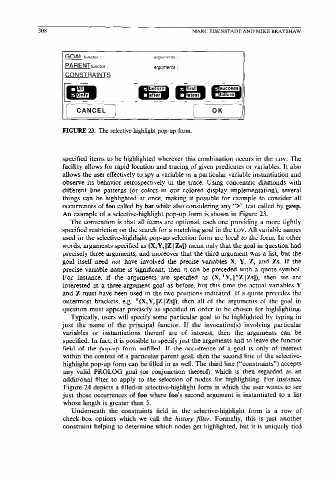
Frequently a user will wish to ask queries of the form, “Where did a given variable get instantiated to value X?” or “Where in the program does foo get called by bar?” To address this problem we provide a selective-highlighting option in the LDV
display. This option allows the user to specify a given pattern, the name of a
predicate, the name of a variable, an instantiated variable term, or any combination thereof, with the further option of specifying a particular parent goal for the pattern to have, if required. The result of such a request is for the nodes that correspond to such a description to be highlighted in the LDV diagram. For example, we can request the highlighting of all occurrences of the predicate foo with a second argument instantiated to the list [bar], and moreover just those occurrences when foo was called by the mother goal gawp. The result of such a request will be for the
308 MARC EISENSTADT AND MIKE BRAYSHAW
GOAL functor :
PARENTrunctor :
CONSTRAINTS
arguments :
arguments :
1 CANCEL 1 I OK
FIGURE 23. The selective-highlight pop-up form.
specified items to be highlighted wherever this combination occurs in the LDV. The facility allows for rapid location and tracing of given predicates or variables. It also allows the user effectively to spy a variable or a particular variable instantiation and observe its behavior retrospectively in the trace. Using concentric diamonds with different line patterns (or colors in our colored display implementation), several things can be highlighted at once, making it possible for example to consider all occurrences of foo called by bar while also considering any 9” test called by gawp. An example of a selective-highlight pop-up form is shown in Figure 23.
The convention is that all items are optional, each one providing a more tightly specified restriction on the search for a matching goal in the LDV. All variable names used in the selective-highlight pop-up selection form are local to the form. In other words, arguments specified as (X, Y, [Z 1 Zsl) mean only that the goal in question had precisely three arguments, and moreover that the third argument was a list, but the goal itself need not have involved the precise variables X, Y, Z, and Zs. If the precise variable name is significant, then it can be preceded with a quote symbol. For instance, if the arguments are specified as (X, ’ Y, [ ’ Z 1 Zs]), then we are interested in a three-argument goal as before, but this time the actual variables Y and Z must have been used in the two positions indicated. If a quote precedes the outermost brackets, e.g. ‘(X,Y, [Z [Zs]), then all of the arguments of the goal in question must appear precisely as specified in order to be chosen for highlighting.
Typically, users will specify some particular goal to be highlighted by typing in just the name of the principal functor. If the invocation(s) involving particular variables or instantiations thereof are of interest, then the arguments can be specified. In fact, it is possible to specify just the arguments and to leave the functor field of the pop-up form unfilled. If the occurrence of a goal is only of interest within the context of a particular parent goal, then the second line of the selective- highlight pop-up form can be filled in as well. The third line (“constraints”) accepts any valid PROLOG goal (or conjunction thereof), which is then regarded as an additional filter to apply to the selection of nodes for highlighting. For instance, Figure 24 depicts a filled-in selective-highlight form in which the user wants to see just those occurrences of foo where foe’s second argument is instantiated to a list whose length is greater than 5.
Underneath the constraints field in the selective-highlight form is a row of check-box options which we call the history jilter. Formally, this is just another constraint helping to determine which nodes get highlighted, but it is uniquely tied
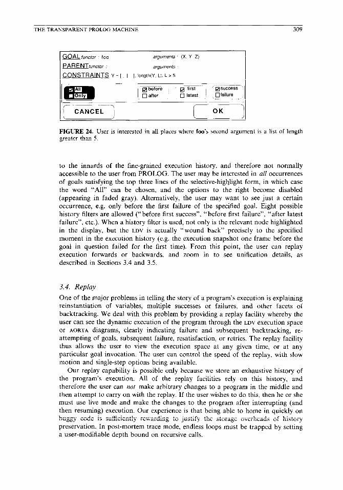
THETRANSPARENTPROLOGMACHINE 309
GOAL functor : foe arguments : (X. Y, 2)
PARENTfuncror : arguments
CONSTRAINTS Y = [ _ 1~ I, length(Y, L), L > 5
FIGURE 24. User is interested in all places where foo’s second argument is a list of length greater than 5.
to the innards of the fine-grained execution history, and therefore not normally accessible to the user from PROLOG. The user may be interested in all occurrences of goals satisfying the top three lines of the selective-highlight form, in which case the word “All” can be chosen, and the options to the right become disabled (appearing in faded gray). Alternatively, the user may want to see just a certain occurrence, e.g. only before the first failure of the specified goal. Eight possible history filters are allowed (“before first success”, “before first failure”, “after latest failure”, etc.). When a history filter is used, not only is the relevant node highlighted in the display, but the LDV is actually “wound back” precisely to the specified moment in the execution history (e.g. the execution snapshot one frame before the goal in question failed for the first time). From this point, the user can replay execution forwards or backwards, and zoom in to see unification details, as described in Sections 3.4 and 3.5.
3.4. Replay
One of the major problems in telling the story of a program’s execution is explaining reinstantiation of variables, multiple successes or failures, and other facets of backtracking. We deal with this problem by providing a replay facility whereby the user can see the dynamic execution of the program through the LDV execution space or AORTA diagrams, clearly indicating failure and subsequent backtracking, re- attempting of goals, subsequent failure, resatisfaction, or retries. The replay facility thus allows the user to view the execution space at any given time, or at any particular goal invocation. The user can control the speed of the replay, with slow motion and single-step options being available.
Our replay capability is possible only because we store an exhaustive history of the program’s execution. All of the replay facilities rely on this history, and therefore the user can not make arbitrary changes to a program in the middle and then attempt to carry on with the replay. If the user wishes to do this, then he or she must use live mode and make the changes to the program after interrupting (and then resuming) execution. Our experience is that being able to home in quickly on buggy code is sufficiently rewarding to justify the storage overheads of history preservation. In post-mortem trace mode, endless loops must be trapped by setting a user-modifiable depth bound on recursive calls.
310 MARCEISENSTADTANDMIKEBRAYSHAW
Typically we would expect the replay facility to be used when the user is trying to figure out why a piece of code behaved as it did in a particular instance and wishes to step through it in simulated execution mode. This is true especially when the user, in figuring out a complex case of backtracking, wishes to find out where final or interim instantiations came about. The user can tell the program to stop at a particular point, which may either be prespecified or else indicated via a mouse click at any point during the dynamic replay. The utility thus allows the user effectively to freeze the program at any step of its execution and use any of the other existing tools on the program at that point, to step backwards or forwards one or more “frames”, or to carry on with the execution.
Just before replay begins (i.e. following a selective highlighting choice or a
request to replay from the beginning), the LDV is “wound back” to the user-selected
point. The interesting thing about the LDV at this point is that it shows a “pre-
ordained” execution space, i.e. nodes in the tree which TPM guarantees will eventu-
ally form part of the execution space, but which at the moment of replay have yet to be
traversed. This provides a context within which the user can watch execution unfold, and is considerably more constrained than the full-blown search space would be. The replay control panel (which is always visible to the user) can then be used to initiate the actual replay.
On a color display we use green nodes to represent success, and red ones failure. Nodes on the active or pending goal stack are indicated by their distinctive (thick-outline) shape. A typical replay scenario runs as follows: the “preordained” LDV changes to indicate the initial area of execution, followed by nodes turning green to indicate success. The execution tree is engulfed in a swathe of green, with isolated patches of red denoting local failures. However, on encountering backtrack- ing, the successful green nodes are retried and turn pink on failure. In the event of extensive backtracking which eventually succeeds, we see large areas of green turn to pink until finally the process stops and the green starts to regain its lost territory. The whole process can be stopped and frozen at an instant to allow for closer
inspection by a mouse click. What is most important here is for the gestalt to be right, i.e. for the display not
only to be informative, but also to feel like an accurate version of the underlying PROLOG machine.
3.5. Zooming
Zooming links the LDV and AORTA representations by allowing the user to switch between the two, enabling the user to zoom in on the unification history of particular clauses from the LDV. In this way the complementary nature of the two views is emphasized. The LDV allows the user to view the program from a clear perspective, uncluttered by unwanted information, and explore its behavior in an orderly, informed manner. The AORTA diagrams as described in Section 2 show the overall success/failure information, as in the LDV, with the additional detail regarding the finally invoked clause body, its matching head, and the other clauses that matched, and their history. Switching from the LDV of a particular node to the AORTA view thus increases the amount and type of information available to the user. Not only is this AORTA view useful for teaching novices, but it also (in conjunction

THETRANSPARENTPROLOGMACHINE 311
with the LDV and zooming) allows the expert rapid and easy access to a large amount of unification history and surrounding information.
The close-up view shows not only the focused-upon goal, but also that goal’s mother, sisters, stepsisters, and daughters. It thus provides both clarity of detail and some surrounding context within which to perform debugging. We call this our three-ply close-up uiew, because three generations of goals are visible at once. The replay facilities described in Section 3.4 are also available in the close-up view, which means that the precise details of unification history can be observed if
necessary. The collection of facilities mentioned above allows the user, whether novice or
expert, to be told much more detail about the history of program execution. Since zooming and highlighting requests always begin with the LDV, all the perspective information associated with the LDV is available at the point of choice, allowing the user clearly to understand the context of the code which is being observed close up. This approach removes the “forest-versus-trees” problem associated with conven- tional “spy” packages. In such packages, once a “spied” goal is reached, it may no longer be clear how one arrived there, how the instantiations of the variables have been derived, what state the program is in, what side effects have taken place, whether the program has only reached this point on backtracking, or (if a “redo” is involved) the nature, cause, and scope of the backtracking involved. By the combi- nation of the LDV, AORTA, zooming, selective highlighting, and replay facilities, the user may more readily understand the state of the program, and thus arrive rapidly at the source of problematic bugs.
Section 4 illustrates the facilities in greater detail by presenting worked examples.
4. WORKED EXAMPLES
To illustrate some of the features of our notation and the environment in which it is embedded, we present several PROLOG programs and show how they are dealt with by TPM. Sections 4.1-4.3 contain examples of code which we consider to be representative of situations we have observed during the writing and debugging of large PROLOG programs. Section 4.1 illustrates TPM’s long-distance-view and selective-highlighting features, applied in the context of a small expert system. Section 4.2 illustrates the role of selective highlighting and zooming in debugging a database manipulation program. Finally, Section 4.3 illustrates how the replay facility is used in debugging a soLo-to-PROLOG compiler.
4.1. An Expert System (Showing LDV, Quick Zoom, Quick Label, and Selective Highlighting)
Although space precludes the discussion of extremely large programs, it is useful to look in some detail at an expert-system example, devised originally by Winston [28] and adapted for PROLOG by Coelho, Cotta, and Pereira [4]. Representative portions of the code are shown in Figure 25. Only selected portions of the database are shown, with ellipsis dots (“. . . “) indicating “more of the same type of code”.
Figure 26 shows the LDV of program execution given the query ?-recognition(animal). In this case, the user has typed a “yes” response to each
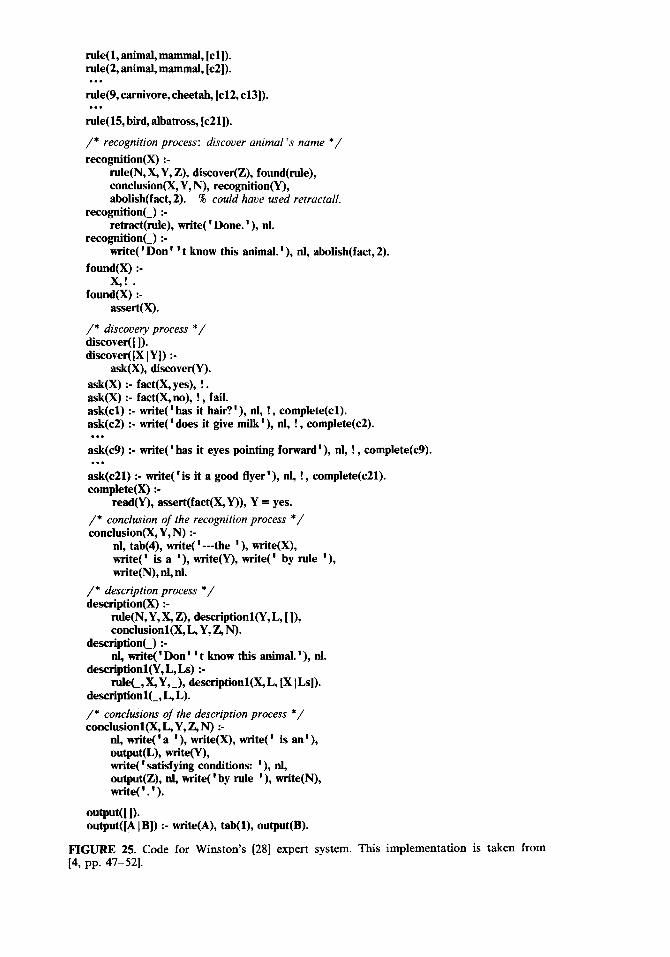
rufe( 1, animal, mammal, [cl]). rule(2, animal, mammal, [c2]). . . .
rule(9, carnivore, cheetah, 1~12, ~131). . . .
rule(l5, bird, albatross, [c21]).
/* recognition process: discover animal’s name */
recognition(X) :- rule(N, X, Y, Z), discover(Z), found(nde), conclusion(X, Y, N), recognition(Y), abolish(fact, 2). 5% could have used retractall.
recognition(_) :- retract(rule), write( ’ Done. ’ ), nl.
recognition(_) :- write( ‘Don ’ ’ t know this animal. ’ ), nl, abofish(fact, 2).
found(X) :- X! .
found(X) :- assert(X).
/* discovey process */ discover( [ I). discover( [x 1 Y]) :-
ask(X), discover(Y).
ask(X) :- fact(X, yes), ! . ask(X) :- fact(X, no), ! , fail. ask(c1) :- write( ‘has it hair?‘), nl, ! , complete(c1). ask(c2) :- write( ‘does it give milk’), nl, ! , complete(c2). . . .
ask(c9) :- write(’ has it eyes pointing forward’), nl, ! , complete(c9). . . .
ask(c21) :- write( ‘is it a good flyer ‘), nl, ! , complete(c21). complete(X) :-
read(Y), assert(fact(X,Y)), Y = yes.
/* conclusion of the recognition process */ conclusion(X, Y, N) :-
nl, tab(4), write( ’ ---the ‘), write(X), write(’ is a ‘), write(Y), write(’ by rule ‘), write(N), nl, nl.
/* description process */ description(X) :-
rule(N,Y,X, Z), descriptionl(Y, L, [I), conclusionl(X, L, Y, Z, N).
description(_) :- nl, write( ‘Don ’ ’ t know this animal. ‘), nl.
descrfptionl(Y, L, Ls) :- rufec, X, Y, _), descriptionl(X, L, [x 1 Ls]).
description&L, L).
/* conclusions of the description process */ conclusionl(X, L, Y, Z, N) :-
nl, tite( ’ a ‘), write(X), write( ’ is an ’ ), output(L), write(Y), write( ’ satisfying conditions: ’ ), nl, output(Z), nf, write( ‘by rule ’ ), write(N), write(‘.‘).
output(] I). output([A 1 B]) :- write(A), tab(l), output(B).
FIGURE 25. Code for Winston’s [28] expert system. This implementation is taken from [4, pp. 47-521.

A

314 MARCEISENSTADTANDMIKEBRAYSHAW
discover([ X 5d YSO ] ) Quick Zoom Viewport
FIGURE 27. Selective highlighting of the place where discover gets called with a multi- element list as its argument. The highlighted node (shown with a diamond surrounding it) is in the fourth tier of goals in the tree. The quick-zoom display at the top reveals that the list passed in to discover at this point is in fact [c12,c13].
question, so that the conclusion was that the animal was a cheetah. The “show LDV
predicates” option is disabled; hence the tree is drawn without predicate names. However, using the “quick label” option introduced in Section 3, we have labeled individually a few nodes in the LDV for convenience. Notice the telltale shape of the tree every time recognition is called.
From the code in Figure 25 we can see that a rule may lead to single or multiple conclusions. The predicate that deals with this is discover. Suppose that we wish only to focus on the time(s) when discover gets called with a multiitem list passed in as its argument, i.e. when we are dealing with multiple conclusions. To highlight the node we use the selective-highlight pop-up form and specify that we want to see the predicate discover called with more than a one-element list e.g. [_, _ 1 ] anywhere where this combination occurs. The node in the diamond in Figure 27 shows the highlighted node. To quickly get a better view we change the function of the right mouse button to quick zoom, using the LDV pop-up menu. If we now mouse-click on the highlighted node, the result is shown in the quick-zoom viewport at the very top of the graphics area. The result of the quick zoom has been to draw the AORTA
procedure status box for the highlighted node. In this example, TPM was used just to confirm that the program was working as
expected. In the upcoming examples, we see how TPM can be used to home in on buggy code.
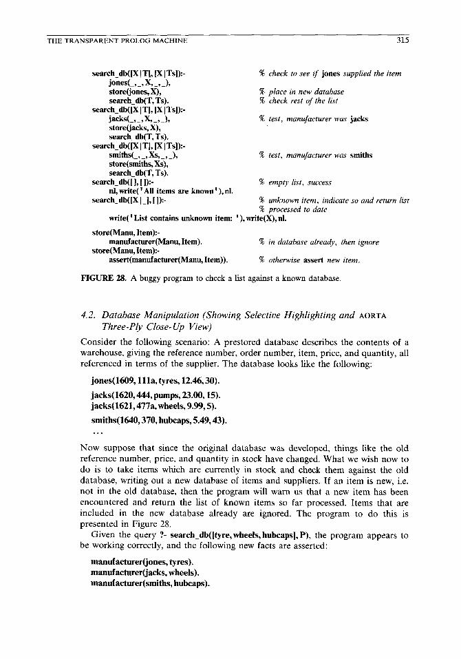
THE TRANSPARENT PROLOG MACHINE 315
==ch_db(B IV, (x I W:- jones(_, _, X, _, J, storetiones, X), search_db(T,Ts).
search_db( Ix ) T], m 1 Ts]):- jaeK,_,X_,_), store(jacks, X), search_db(T, Ts).
search_db(fi 1 T], p 1 Ts]):- smitK_,Xs,_,_), store(smiths, Xs), search_db(T, Ts).
-rch_db(I I,[ I):- nl, write( ‘All items are known ’ ), nl.
=reh._db([X IA, I I):-
% check to see if jones supplied the item
% place in new database % check rest of the list
% test, manufacturer was jacks
% test, manufacturer was smiths
% empty list, success
% unknown item, indicate so and return list % processed to date
write( ’ List contains unknown item: ’ ), write(X), nl.
store(Manu, Item):- manufacturer(Manu, Item). % in database already, then ignore
store(Manu, Item):- assert(manufacturer(Manu, Item)). % otherwise assert new item.
FIGURE 28. A buggy program to check a list against a known database.
4.2. Database Manipulation (Showing Selective Highlighting and AORTA
Three-Ply Close- Up View)
Consider the following scenario: A prestored database describes the contents of a warehouse, giving the reference number, order number, item, price, and quantity, all referenced in terms of the supplier. The database looks like the following:
jones(1609, llla, tyres, 12.46,30).
jacks( 1620,444, pumps, 23.00,15). jacks(1621,477a, wheels, 9.99,5).
smiths( 1640,370, hubcaps, 5.49,43). . . .
Now suppose that since the original database was developed, things like the old reference number, price, and quantity in stock have changed. What we wish now to do is to take items which are currently in stock and check them against the old database, writing out a new database of items and suppliers. If an item is new, i.e. not in the old database, then the program will warn us that a new item has been encountered and return the list of known items so far processed. Items that are included in the new database already are ignored. The program to do this is presented in Figure 28.
Given the query ?- search db([tyre, wheels, hubcaps], P), the program appears to be working correctly, and the-following new facts are asserted:
manufacturer(jones, tyres). manufacturer(jacks, wheels). manufacturer(smiths, hubcaps).
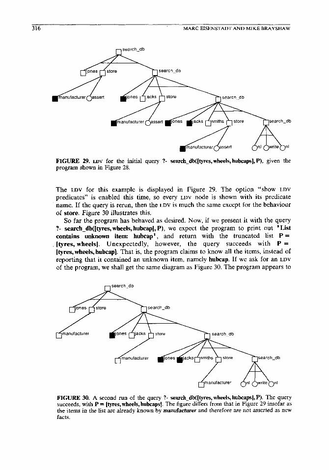
316 MARC EISENSTADT AND MIKE BRAYSHAW
‘h search_db
FIGURE 29. LDV for the initial query ?- search_db( [tyres, wheels, hubcaps], P), given the program shown in Figure 28.
The LDV for this example is displayed in Figure 29. The option “show LDV
predicates” is enabled this time, so every LDV node is shown with its predicate name. If the query is rerun, then the LDV is much the same except for the behaviour of store. Figure 30 illustrates this.
So far the program has behaved as desired. Now, if we present it with the query ?- search_db([tyres, wheels, hubcap], P), we expect the program to print out ‘List contains unknown item: hubcap ’ , and return with the truncated list P = [tyres, wheels]. Unexpectedly, however, the query succeeds with P = [tyres, wheels, hubcap]. That is, the program claims to know all the items, instead of reporting that it contained an unknown item, namely hubcap. If we ask for an LDV
of the program, we shall get the same diagram as Figure 30. The program appears to
FIGURE 30. A second run of the query ?- search_db([tyres, wheels, hubcaps], P). The query succeeds, with P = [tyres, wheels, hubcaps]. The figure differs from that in Figure 29 insofar as the items in the list are already known by manufacturer and therefore are not asserted as new facts.

THETRANSPARENTPROLOGMACHINE 317
search_db GOAL functor :
PARENTruncm :
CONSTRAINTS
arguments : ( [hubcap I_] , _ )
arguments :
FIGURE 31. We’ve asked to see the call to search_db highlighted when its first argument is instantiated to some list beginning with hubcap, and we want to see all possible occurrences.
have behaved in the same manner. Since we are interested in what happened when search_db came to deal with hubcap, we can use the selective-highlight facility to show us everywhere in the tree search_db gets called with first argument instantiated to [hubcap 1-1, as shown in Figure 31. Notice that, having set the history filter to “all”, we now cannot choose before/after, first/latest, or success/failure; hence these check-box options are shown faded, indicating that they are passive to mouse clicks. The result of our highlighting request is shown in Figure 32.
Having located this node, we can ask TPM to zoom in on the goal. As Figure 33 shows, this gives us a three-ply view of the goal, with the chosen goal in the middle of the AORTA diagram. The AORTA diagram initially appears with the arguments of only the zoomed-upon node displayed, but by menu selection any other node may also have its arguments displayed. In the snapshot shown in Figure 33 the procedure status boxes for smiths and store have been selected for full-argument display. From the AORTA diagram we can see that the program’s behavior prior to reaching the chosen goal was entirely as predicted. Once attempting the goal, it tries to prove clause 1 of search_db but fails. Clause 2 is then attempted, but this also fails. This is what is expected. However, we can see that the first subgoal (smiths) in the body of
FIGURE 32. LDV of the query ?- search_db( [tyres, wheels, hubcap], P), which unexpectedly succeeded. The goal searcb_db with first argument [hubcap I_] is highlighted.
m search_db
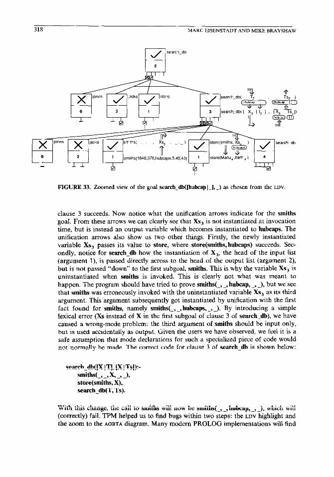
318 MARCEISENSTADTANDMIKEBRAYSHAW
search_db( [ X, / T3 ] ,
smiths(1640,370.hubcaps,5.49,43)
Q ’ ’ I I I I t
FIGURE 33. Zoomed view of the goal search_db((hubcapl_],_) as chosen from the LDV.
clause 3 succeeds. Now notice what the unification arrows indicate for the smiths goal. From these arrows we can clearly see that Xs, is not instantiated at invocation time, but is instead an output variable which becomes instantiated to hubcaps. The unification arrows also show us two other things. Firstly, the newly instantiated variable Xs, passes its value to store, where store(smiths, hubcaps) succeeds. Sec- ondly, notice for search_db how the instantiation of X,, the head of the input list (argument l), is passed directly across to the head of the output list (argument 2), but is not passed “down” to the first subgoal, smiths. This is why the variable Xs, is uninstantiated when smiths is invoked. This is clearly not what was meant to happen. The program should have tried to prove smiths(_, _, hubcap, _, _), but we see that smiths was erroneously invoked with the uninstantiated variable Xs, as its third argument. This argument subsequently got instantiated by unification with the first fact found for smiths, namely smiths(_,_, hubcaps,_,_). By introducing a simple
lexical error (Xs instead of X in the first subgoal of clause 3 of search_db), we have caused a wrong-mode problem: the third argument of smiths should be input only, but is used accidentally as output. Given the users we have observed, we feel it is a safe assumption that mode declarations for such a specialized piece of code would not normally be made. The correct code for clause 3 of search_db is shown below:
search_db([X IT], [X 1 Ts]):-
smiths(_, _, X, _, _), store(smiths, X), search_db(T, Ts).
With this change, the call to smiths will now be smiths(_, _, hubcap,_,_), which will (correctly) fail. TPM helped us to find bugs within two steps: the LDV highlight and
the zoom to the AORTA diagram. Many modem PROLOG implementations will find
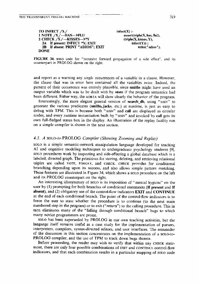
THETRANSPARENTPROLOGMACHINE 319
TO INFECT /X/ 1 NOTE /X/---HAS--->FLU 2 CHECK /X/---KISSES--->?Y
2A If present: INFECT *Y; EXIT 2B If absent: PRINT “ADIOS”; EXIT
DONE
infect(X) :- assert(triple(X, has, flu)), (triple(X, kisses, Y),
infect(Y)) ; tite( ’ adios ’ ).
FIGURE 34. SOLO code for “recursive forward propagation of a side effect”, and its counterpart in PROLOG shown on the right.
and report as a warning any single occurrences of a variable in a clause. However, the clause that was in error here contained all the variables twice. Indeed, the pattern of their occurrence was entirely plausible, since smiths might have used an output variable which was to be dealt with by store if the program semantics had been different. Either way, the AORTA will show clearly the behavior of the program.
Interestingly, the more elegant general version of search_db, using “univ” to generate the various predicates (smiths,jacks, etc.) at runtime, is just as easy to debug with TPM. This is because both “univ” and call are displayed as circular nodes, and every runtime instantiation built by “univ” and invoked by call gets its own full-fledged status box in the display. An illustration of the replay facility run on a simple compiler is shown in the next section.
4.3. A som-to-PROLOG Compiler (Showing Zooming and Replay)
SOLO is a simple semantic-network manipulation language developed for teaching AI and cognitive modeling techniques to undergraduate psychology students [9]. SOLO procedures work by inspecting and side-effecting a global database which is a labeled, directed graph. The primitives for storing, deleting, and retrieving relational triples are called NOTE, FORGET, and CHECK. CHECK provides for conditional branching depending upon its success, and also allows simple pattern matching. These features are illustrated in Figure 34, which shows a SOLO procedure on the left and its PROLOG counterpart on the right.
An interesting idiosyncrasy of SOLO is its imposition of “mental hygiene” on the user by (1) prompting for both branches of conditional statements (If present and If absent), and (2) obligatory use of the control-flow indicators EXIT and CONTINUE at the end of each conditional branch. The point of the control-flow indicators is to force the user to state whether the procedure is to continue (to the next main numbered step in the program) or to exit (“return”) to the calling procedure. This in turn eliminates many of the “falling through conditional branch” bugs to which many novice programmers are prone.
SOLO has been superseded by PROLOG in our own teaching activities, but the language itself remains useful as a case study for the implementation of parsers, interpreters, compilers, syntax-directed editors, and user interfaces. The remainder of the discussion in this section concentrates on the implementation of a SOLO-to- PROLOG compiler, and the use of TPM to track down bugs therein.
Before proceeding, the reader may wish to verify that within any CHECK state- ment, there are only four possible combinations of EXIT and CONTINUE control-flow indicators, and that each combination results in a particular mapping of SOLO code

320 MARCEISENSTADTANDMIKEBRAYSHAW
TO JUDGE /X/ 1 CHECK /X/---VOTES---XNDEPENDENT
LA If present: PRINT “AHA, A FREE THINKER”; CONTINUE 1B If absent: PRINT “UH OH: A PUPPET”; EXIT
2 PRINT “WHICH IS ALL RIGHT WITH ME” DONE
FIGURE 35. SOLO code for “criticizing a person’s voting habits”.
onto PROLOG code. These combinations form the basis for the heart of the compiler to be illustrated momentarily. Before getting into the details, let’s look at another SOLO procedure called JUDGE (Figure 35). The equivalent PROLOG code is shown in Figure 36. For expository purposes, we assume a mapping from SOLO
onto a single PROLOG clause containing embedded conjunctions and disjunctions. In our actual implementation, we include a puriJer which converts potentially awful embeddings into easier-to-follow multiclause definitions.
The details of the SOLO user interface and the front-end parsing routines (developed in our laboratory by Tony Hasemer) are not relevant to the current discussion, so we just take it as given that the SOLO program shown in Figure 35 can be parsed into the internal representation (i.e. SOLO code depicted in the form of a PROLOG structure) shown in Figure 37. We use the predicate solodef with two arguments: the name of the SOLO procedure (including its arguments, if any), and a list of lists containing the main steps of the SOLO procedure in order. CHECK
statements are represented as six-element lists containing:
(1) the key word check,
(2) the triple which needs to be looked up in the database,
(3) the action to perform if the triple is present,
(4) what to do after (3), i.e. exit or continue,
(5) the action to perform if the triple is absent,
(6) what to do after (5), i.e. exit or continue.
Converting a procedure from SOLO to PROLOG is now a matter of retrieving its definition, and doing some pattern matching to detect the different possible control-flow combinations involving CHECK. Below we show a workhorse predicate called compile which does this. Our top-level driver is called convert. It uses an auxiliary predicate called when enabled which conditionally (i.e. when an appropri- ate enabled assertion is stored in the database) performs some action for the user’s benefit, such as listing code on the terminal. When the appropriate body of the
FIGURE 36. PROLOG version of the SOLO code presented in Figure 35. Single-clause definition is produced deliberately.
judge(X) :- (triple(X, votes, independent),
write( ‘aha: a free thinker’), write( ‘which is all right with me ‘)) ;
write( ‘uh oh: a puppet’).

THETRANSPARENTPROLOGMACHINE 321
solodef(judge(X), I [check,
[x, votes, independent], [print, ‘aba: a free thinker’], cant, Iprint , ’ uh oh: a puppet ’ 1, exit],
[print, ‘which is all right with me’] I).
FIGURE 37. Internal representation of SOLO code shown in Figure 35. The parser itself is not discussed in this paper.
definition is obtained by instantiating the variable PrologCode in compile, the head and body are both asserted into the database. A listing of the top-level driver is shown in Figure 38.
The workhorse predicate compile, defined in Figure 39, takes a list of SOLO
statements as its input (first argument), and returns a PROLOG clause body as its output (second argument). Typically, the SOLO code for either the “if present” branch (Prescode) or the “if absent” branch (Abscode) also needs to be converted to PROLOG. There are two possibilities:
(1) A trivial conversion takes place via the predicate decode, which does such things as convert NOTE FIDO ISA DOG to the PROLOG form assert(tri-
ple(fido, isa, dog)).
(2) The SOLO statement itself is part of a longer list of SOLO statements, which can in turn be converted by means of a recursive call to compile. Which branches of SOLO code run together to form a nice PROLOG conjunction is uniquely determined by the four combinations of EXIT/CONTINUE, EXIT/
EXIT, CONTINUE/EXIT, and CONTINUE/CONTINUE.
The SOLO triple JOHN KISSES MARY is converted into the PROLOG form triple(john, kisses, mary) rather than kisses(john, mary) for historical reasons, related
FIGURE 38. Top-level driver and auxiliary predicates for soLo-to-PROLOG compiler.
convert(Pred, PrologCode):- solodef(F+ed, Solo&de), % retrieve dejnition compile(SoloCode, Prolog&de), % map SOLO into PROLOG when_enabled(show_code(Pd, Prolog&de)), % inform user assert((Pred :- Prolog&de)), 9;; put new code in database retract(compiling). % kill old Jag
when_enabled(ACIlON) :- % cute way to do actions conditionally enabled(ACTION), % is there a jag in db allowing us to proceed? call(ACTION). % then perform the action
when_enabled(ACTION). % no Jag? OK-default success (i.e. carry on)
enabled(show_code(_,_)). % Jag to run show-code when requested
show_code(Pred, Body):- write(Pred), write(’ :- ‘), nl, tab(l2), tite(Body).

322 MARC EISENSTADT AND MIKE BRAYSHAW
% FOUR CHECK CASES: EXIT/CONT; EXIT/EXIT; CONT/EXIT; CONT/CONT: compile([[cbeck, [A, B, C], Prescode, exit, Abscode, cent] (Rest], 5% EXIT/CONT
(triple(A, B, C), Thencode ; Elsecode)) :- decode(Prescode, Tbencode), compile([Abscode 1 Rest], Elsecode).
compile([[check, [A, B, C], Prescode, exit, Abscode, exit] (Rest], % EXIT/EXIT (triple(A, B, C), Tbencode ; Elsecode)) :-
decode(Prescode, Tbencode), decode(Abscode, Elsecode).
compile( [[check, [A, B, C], Prescode, con& Abscode, exit] 1 Rest], 5% CONT/EXZT (triple(A, B, CT), Tbencode ; Elsecode)) :-
compile((prescode I Rest], Tbencode), decode(Abscode, Elsecode).
compile([[cbeck, [A,B, C],Prescode,cont,Abscode,cont] IRest], % CONT/CONT ((triple(A,B, C),Tbencode ; Elsecode) , Restcode)) :-
decode(Prescode, Tbencode), decode(Abscode, Ekecode), compile(Rest, Restcode).
% TWO cases not involving check at ail: compile( [[F ( Args] I 01, (Fcode, Ocode)) :-
decode([F I Args], Fcode), compile( 0, Ocode).
compile([ 1, true).
% most general case % convert first part of code trivially % then recurse on rest
decode( [ 1, true). % no code? convert to “true” decode( Iprint, Arg], tite(Arg)). 5% map “print” onto “write” decode([note, A, B, C], assert(triple(A, B, C))). % map “note ” onto “assert ” decode([Any (Rest], PrologPred):- % FOO A B C in SOLO = [ foo, a, 6, c]
PrologPred = . . [Any IRest]. % . . then try your luck with “foo(a, b, c)”
FIGURE 39. Workhorse predicates compile and decode.
to the need to access any part of the triple with equal ease. Figure 39 provides the remainder of the code necessary to continue illustrating TPM in action.
The code shown in Figures 38 and 39 contains a bug. In response to the top level query ?- convert(judge(P),L), not only does the goal fail, but also show-code succeeds multiple times and prints out ten answers rather than just one. Worse still, listing the clauses that now exist for judge, we find there are now twenty (nineteen of which are totally meaningless). If we use TPM to run a post-mortem trace on the same top-level query, it is immediately obvious what has happened. Figure 40 shows the final LDV. On examination of the final LDV, we can see clearly how we came to
backtrack and produce multiple solutions. All the goals can be seen to have succeeded at least once, but to have failed later on backtracking, with the exception of retract(compiling), which is the youngest (rightmost) subgoal of the top-level goal in Figure 40. To confirm this we can select the replay menu option to display the tree precisely as it would have looked at the very point at which the goal retract(compiling) was attempted. This is done using the selective-highlight pop-up form, as shown in Figure 41.
Following the selective highlight shown in Figure 41, the LDV is automatically “wound back” to the point where retract was initially invoked, as the history filter in the selective-highlight pop-up form specified. The LDV at this point shows a preordained execution space, i.e. nodes in the tree which TPM guarantees will
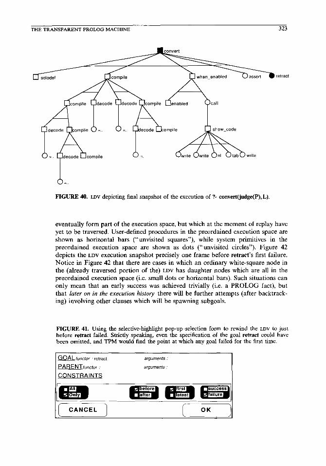
THE TRANSPARENT PROLOG MACHINE 323
retract
compile A =.. de CLrite
FIGURE 40. LDV depicting final snapshot of the execution of ?- convert(judge(P),L).
eventually form part of the execution space, but which at the moment of replay have yet to be traversed. User-defined procedures in the preordained execution space are
shown as horizontal bars (“unvisited squares”), while system primitives in the preordained execution space are shown as dots (“unvisited circles”). Figure 42 depicts the LDV execution snapshot precisely one frame before retract’s first failure. Notice in Figure 42 that there are cases in which an ordinary white-square node in the (already traversed portion of the) LDV has daughter nodes which are all in the preordained execution space (i.e. small dots or horizontal bars). Such situations can only mean that an early success was achieved trivially (i.e. a PROLOG fact), but that later on in the execution history there will be further attempts (after backtrack- ing) involving other clauses which will be spawning subgoals.
FIGURE 41. Using the selective-highlight pop-up-selection form to rewind the LDV to just before retract failed. Strictly speaking, even the specification of the goal retract could have been omitted, and TPM would find the point at which any goal failed for the first time.
GOAL /uncror : retract
PARENTfmror :
CONSTRAINTS
arguments :
arguments :
11 CANCEL 1 r OK II
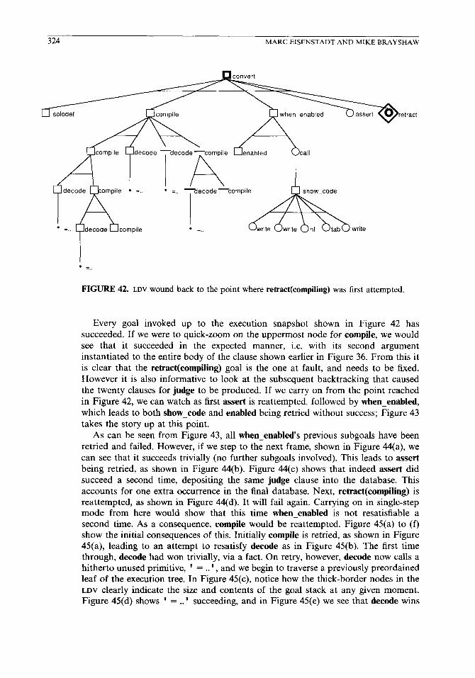
324 MARC EISENSTADT AND MIKE BRAYSHAW
retract
FIGURE 42. LDV wound back to the point where retract(compiling) was first attempted.
Every goal invoked up to the execution snapshot shown in Figure 42 has succeeded. If we were to quick-zoom on the uppermost node for compile, we would see that it succeeded in the expected manner, i.e. with its second argument instantiated to the entire body of the clause shown earlier in Figure 36. From this it is clear that the retract(compiling) goal is the one at fault, and needs to be fixed. However it is also informative to look at the subsequent backtracking that caused the twenty clauses for judge to be produced. If we carry on from the point reached in Figure 42, we can watch as first assert is reattempted, followed by when enabled, which leads to both show-code and enabled being retried without success; Figure 43 takes the story up at this point.
As can be seen from Figure 43, all when-enabled’s previous subgoals have been retried and failed. However, if we step to the next frame, shown in Figure 44(a), we can see that it succeeds trivially (no further subgoals involved). This leads to assert being retried, as shown in Figure 44(b). Figure 44(c) shows that indeed assert did succeed a second time, depositing the same judge clause into the database. This accounts for one extra occurrence in the final database. Next, retract(compiling) is reattempted, as shown in Figure 44(d). It will fail again. Carrying on in single-step mode from here would show that this time when enabled is not resatisfiable a second time. As a consequence, compile would be reattempted. Figure 45(a) to (f) show the initial consequences of this. Initially compile is retried, as shown in Figure 45(a), leading to an attempt to resatisfy decode as in Figure 45(b). The first time through, decode had won trivially, via a fact. On retry, however, decode now calls a hitherto unused primitive, ’ = . . ’ , and we begin to traverse a previously preordained
leaf of the execution tree. In Figure 45(c), notice how the thick-border nodes in the LDV clearly indicate the size and contents of the goal stack at any given moment. Figure 45(d) shows ’ = ..I succeeding, and in Figure 45(e) we see that decode wins

THE TRANSPARENT PROLOG MACHINE 325
retract
=.. Yecode-complle
FIGURE 43. LDV replayed to the point where when-enabled is being retried but the previous clause’s subgoals, show-code and enabled, have failed on backtracking.
anew. Examination of the LDV node for decode via a quick zoom would show that this success is due to clause 4. The final execution snapshot in this sequence, Figure 45(f), shows compile succeeding yet again.
Thus we can use the replay facility to trace and find the source of resatisfaction of a backtracking program. From the above we can see that each time decode initially wins on clause 2, it can be retried and succeed incorrectly a second time on clause 4 (it also wins on clause 4 anyway in the example). If we were to follow this through, we would also observe that when compile succeeds on clause 3, on backtracking it may be resatisfied on clause 5, bringing back an incorrect answer. The user could have prevented this behavior by placing “green” cuts in clauses 2 and 3 of decode, clause 1 of when-enabled, and clauses l-4 of compile, to indicate their determinacy.
5. CODE ABSTBACTIONS
Even given our commitment to telling the truth about the procedural side of PROLOG, and our belief in the power of gestalt patterns in viewing large execution spaces, there are cases in which the user may not wish to know about certain execution details, either because a lump of code is tried and tested, or because it is not relevant to the problem at hand. What is frequently needed is a way of abstracting away from some of the low-level details.
We have extended our notation to deal with four different kinds of abstractions that we believe to be of central importance to the functioning of a practical trace

326 MARC EISENSTADT AND MIKE BRAYSHAW
retract
l =__ decode Ucompile l =._ Grita (&rite OnI UtabWwrite
(a)
fert
retract
” decode
l =..
(b)
FIGURE 44. Four successive LDV replay snapshots: (a) The goal when-enabled succeeds trivially a second time when it is retried. (b) A new call is made to the assert goal. (c) The assert goal succeeds. (d) A new call is made to the retract goal.
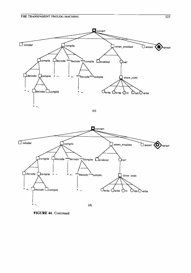
THE TRANSPARENT PROLOG MACHINE 327
retract
w
x complle Ydecode IecodeTmpile Uenabled 5 7 call
l =.. Yecode-compile
! =_.
l =.. (4
FIGURE 44. Continued
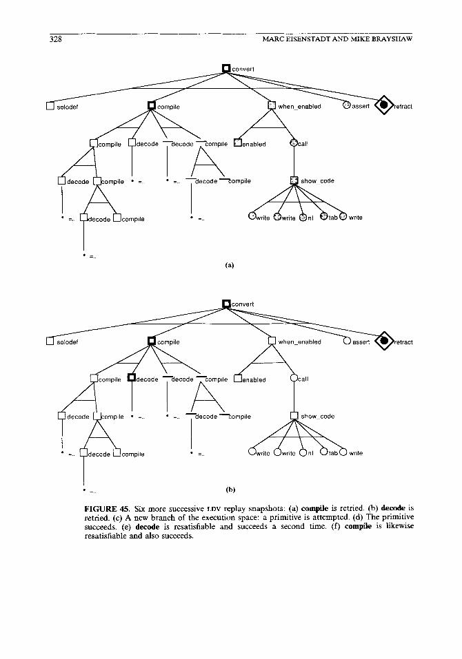
328 MARC EISENSTADT AND MIKE BRAYSHAW
retract
(a)
’ =.. l+lecade klcompile ’ =.. CLrite &rite bnl
(b)
-0 retract
FIGURE 45. Six more successive LDV replay snapshots: (a) compile is retried. (b) decode is retried. (c) A new branch of the execution space: a primitive is attempted. (d) The primitive succeeds. (e) decode is resatistiable and succeeds a second time. (f) compile is likewise resatisfiable and also succeeds.

THE TRANSPARENT PROLOG MACHINE 329
decode %ompile
I A
aenabled
l =.. decode compile
‘m write l =.. !_$decode Ucompile
I l =..
Cc)
’ =.. decode ‘-Compile
compile
l =..
(4
FIGURE 45. Continued
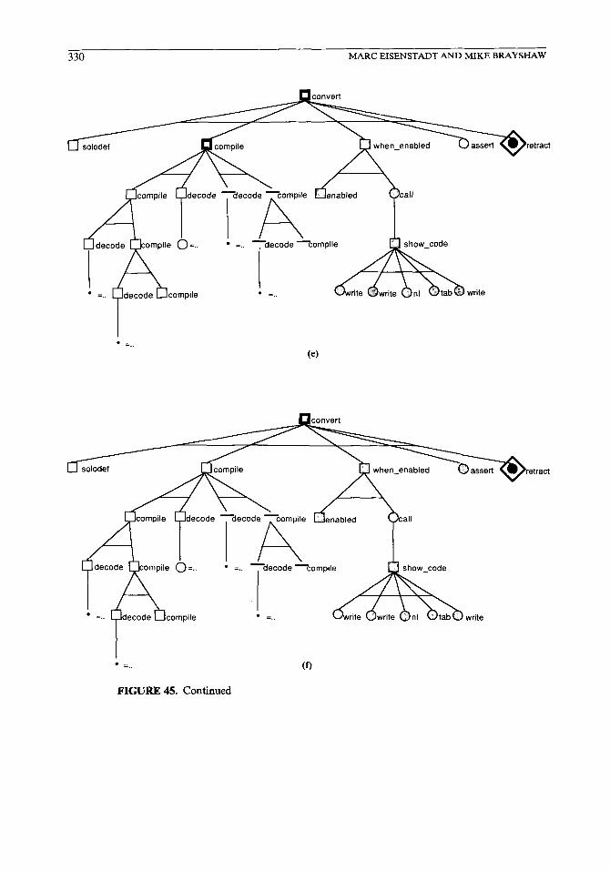
330 MARC EISENSTADT AND MIKE BRAYSHAW
retract
W
retract
FIGURE 45. Continued
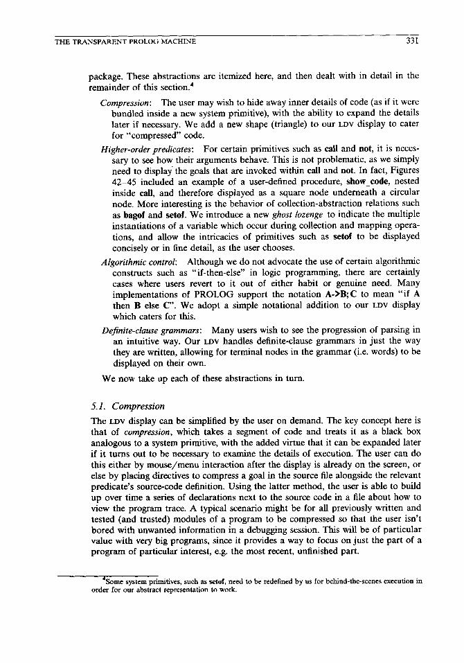
THETRANSPARENTPROLOGMACHINE 331
package. These abstractions are itemized here, and then dealt with in detail in the remainder of this section4
Compression: The user may wish to hide away inner details of code (as if it were bundled inside a new system primitive), with the ability to expand the details later if necessary. We add a new shape (triangle) to our LDV display to cater for “compressed” code.
Higher-order predicates: For certain primitives such as call and not, it is neces- sary to see how their arguments behave. This is not problematic, as we simply need to display the goals that are invoked within call and not. In fact, Figures 42-45 included an example of a user-defined procedure, show_code, nested inside call, and therefore displayed as a square node underneath a circular node. More interesting is the behavior of collection-abstraction relations such as bagof and setof. We introduce a new ghost lozenge to indicate the multiple instantiations of a variable which occur during collection and mapping opera- tions, and allow the intricacies of primitives such as setof to be displayed concisely or in fine detail, as the user chooses.
Algorithmic control: Although we do not advocate the use of certain algorithmic constructs such as “if-then-else” in logic programming, there are certainly cases where users revert to it out of either habit or genuine need. Many implementations of PROLOG support the notation A-X&C to mean “if A then B else C”. We adopt a simple notational addition to our LDV display which caters for this.
Definite-clause grammars: Many users wish to see the progression of parsing in an intuitive way. Our LDV handles definite-clause grammars in just the way they are written, allowing for terminal nodes in the grammar (i.e. words) to be displayed on their own.
We now take up each of these abstractions in turn.
5. I. Compression
The LDV display can be simplified by the user on demand. The key concept here is that of compression, which takes a segment of code and treats it as a black box analogous to a system primitive, with the added virtue that it can be expanded later if it turns out to be necessary to examine the details of execution. The user can do this either by mouse/menu interaction after the display is already on the screen, or else by placing directives to compress a goal in the source file alongside the relevant predicate’s source-code definition. Using the latter method, the user is able to build up over time a series of declarations next to the source code in a file about how to view the program trace. A typical scenario might be for all previously written and tested (and trusted) modules of a program to be compressed so that the user isn’t bored with unwanted information in a debugging session. This will be of particular value with very big programs, since it provides a way to focus on just the part of a program of particular interest, e.g. the most recent, unfinished part.
4Some system primitives, such as setof, need to be redefined by us for behind-the-scenes execution in order for our abstract representation to work.
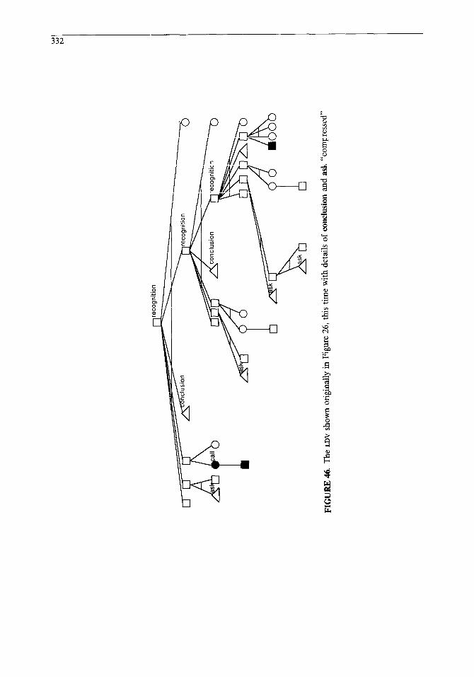
332
I\ -

THETRANSPARENTPROLOGMACHINE 333
The user can instruct TPM to throw away information which would otherwise allow retroactive expansion of compressed nodes. This option allows the user to benefit from increased execution speed (since “compressed” goals can simply be proved without additional tracer history storage overheads). Of course, the user must weigh this benefit against the loss of potentially valuable debugging informa- tion. In the case of well-tried and robust code the user may deem this worthwhile.
In Figure 46 we see the LDV display shown earlier in Figure 26 with the nodes corresponding to invocations of conclusion and ask “compressed” into single triangular-shaped nodes. The shading conventions for success, failure, etc., remain consistent across all LDV nodes, regardless of shape. If the user chooses to expand such compressed nodes, the previous LDV with the still-compressed nodes is pre- served in a small viewport at the top of the display to provide some useful contextual cues.
5.2. Higher-Order Predicates: setof
Higher-order predicates such as setof pose a particularly challenging problem to the designer of a trace package. One could always “hand-code” setof, and then just show the full blown details using TPM’s existing tracing facilities, or even use the
compress option described in Section 5.1. However, such a solution is not represen- tative of the very abstraction which setof was designed to capture. Indeed, setof was meant to liberate the user from the tedium of having to design and implement low-level iteration/collection cliches by hand, so a brute-force trace of the hand- coded implementation of setof would be something of a retrograde step.
Our solution is to use the concepts and notation we have already developed, but to make it expressive at the appropriate level of abstraction. We shall use a single piece of code and several different invocations of setof to illustrate the notation. The code, shown in Figure 47, is meant to designate the nodes and links in an arbitrary directed graph. Now consider the following query, which retrieves all node-node links:
?- setof(X-Y, arc(X, Y), Ans). Ans = [a-b, a-c, b-c, b-d, c-d] x= -310 Y= -311
The AORTA diagram representation of the above interaction is shown in Figure 48. Here are the important things to note about Figure 48:
The large arrow underneath the circle indicates that this particular higher-order primitive obtains multiple solutions from its lower-order predicate (in this case arc). The details of the execution of the lower-order predicate can be obtained
FIGURE 47. A database showing how nodes a, b, c, and d are linked in a directed graph.
da, W. da, cl. arc(b, c). arc(c, d). arc(b, d).
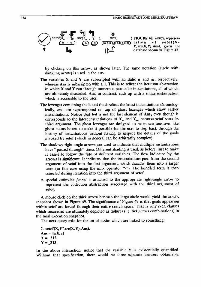
334 h4ARCEISENSTADTANDMIKEBRAYSHAW
) FIGURE 48. AORTA represen- ta tie n 0 f setof(X- Y, arc@, Y), Am), given the database shown in Figure 47.
by clicking on this arrow, as shown later. The same notation (circle with dangling arrow) is used in the LDV.
The variables X and Y are subscripted with an italic n and m, respectively, whereas Ans is subscripted with a 1. This is to reflect the iteration abstraction in which X~and Y run through numerous particular instantiations, all of which are ultimately discarded. Am, in contrast, ends up with a single instantiation which is accessible to the user.
The lozenges containing the b and the d reflect the latest instantiations chronolog- ically, and are superimposed on top of ghost lozenges which show earlier instantiations. Notice that b-d is not the last element of Ans, even though it corresponds to the latest instantiations of X, and Y,,,, because setof sorts its third argument. The ghost lozenges are designed to be mouse-sensitive, like ghost status boxes, to make it possible for the user to step back through the history of instantiations without having to inspect the details of the goals invoked by setof (which in general can be arbitrarily complex).
The shadowy right-angle arrows are used to indicate that multiple instantiations have “passed through” them. Different shading is used, as before, just to make it easier to follow the fate of different variables. The flow indicated by the arrows is significant. It indicates that the instantiations pass from the second argument of setof into the first argument, which bundles them into a larger term (in this case using the infix operator “-“). The bundled term is then collected during iteration into the third argument of setof.
A special collection funnel is attached to the appropriate right-angle arrow to represent the collection abstraction associated with the third argument of &of.
A mouse click on the thick arrow beneath the large circle would yield the AORTA snapshot shown in Figure 49. The significance of Figure 49 is that goals appearing within setof are forced through their entire search space. That is why even clauses which succeeded are ultimately depicted as failures (i.e. tick/cross combinations) in the final execution snapshot.
The next query asks for the set of nodes which are linked to something:
?- setof(X, Y-arc& Y), Ans). Ans = [a, b, c] x= -312 Y= -313
In the above interaction, notice that the variable Y is existentially quantified. Without that specification, there would be three separate answers obtainable,

THE TRANSPARENT PROLOG MACHINE 335
lr )P Ans, 1
[a-b,a-c.b-c,b-d,c-d]
FIGURE 49. More fine- grained view of exhaustive search of are(X,Y), using the same example as that shown in Figure 48.
corresponding to the three different instantiations of Y, as the following interaction shows:
?- setof@, arc@, Y), Ans). Ans = [a] Y=b;
Ans = Ia,b] Y = c;
Ans = [b,c] Y=d; no
The AORTA diagram corresponding to the existentially-quantified query is shown in Figure 50.
Had the existential quantifier notation not been used, Y would have received an ordinary subscript, like Ans, reflecting its role as an ordinary variable which can receive but a single instantiation. As shown in Figure 50, however, Y is subscripted with an italic letter, indicating that it can run through numerous possible instantia- tions.
Since the second argument of setof is an arbitrary (conjunction of) PROLOG goal(s), it is possible to nest setof within setof. The following query uses this idea to retrieve a set of “families”, i.e. nodes and all of the “children” (i.e. recipients of the arc link) of each node:
?- setof(Pa-Kids, setof(K, arc(Pa, K), Kids), Ans). Ans = [a-lb, c], b-[c, d], c-Id] ]
setoft&, kAarc(X, , V, ), Ans, ) b (-g@ ([a,b,cl
FIGURE 50. AORTA representation of
b
setof@, Y^arc(X, y), Am), given the database shown in Figure 47.

336 MARCEISENSTADTANDMIKEBRAYSHAW
setof(Ps -Kids,,, ,setof(Kg ,arc(Ps
0 ._
FIGURE 51. Using setof within setof.
The AORTA representation of the above query is shown in Figure 51. Once again special shadowy unification arrows are needed to indicate the multiplicity of instantiations. This time, we use longer and shorter arrows to indicate the flow of instantiations within and between the respective occurrences of setof. Notice the two collection funnels, and the shadow on the innermost one indicating that this collection itself occurs on more than one iteration.
5.3. Algorithmic Control: If-Then-Else
Whether or not it is a sensible way to write PROLOG code, many users revert to using the syntax A->B; C to implement if-then-else algorithmic control. To illustrate how this control variant is integrated into TPM, consider the problem of retrieving the location of a database Jug whose setting depends upon the particular release of software. In order to find a particular location for a flag, you need first to choose one of several available versions of software. If that version is later than release 7 (say), then you look in a particular set of new locations stored in the database, else you look at some standard default ones. Additionally, suppose that a given location is only of use to you if its flag happens to be set to true. The code to find a good location is shown in Figure 52.
Figure 53(a), (b) show the LDVS corresponding to the processing of the query ?- location(X). The sideways arrow between two subgoal branches separates the “if” branch from the “then” branch, and the thickened tree branch indicates the location of (possibly several conjoined) “then”s. The “then” branch is in turn separated from the “else” branch as an ordinary disjunction. The sideways arrow and thick line together show what amounts to an implicit “cut” in the “if-then-else” construct. In Figure 53(a) we see the execution at the point where the goal flag(5015,true) is about to be attempted. The figure shows that both the “if’ and “then” branches have been successful. However, flag(5015,true) now fails, and backtracking into the “then” branch does not produce any more successful clause matches, so check-version fails (we do not retry the “if” because of the implicit cut). Retrying version produces a different version number, which this time is prior to release 8. Next, there is a new invocation of check-version. This time, the “if” goal (7>7) fails, causing the “else” part of the conditional to be tried. Notice that the “then” branch from the previous invocation of check-version is shown faded, as appropriate for earlier invocations [cf. Figure 18(b)]. The “else” branch succeeds, so check-version succeeds, as does the flag goal, and therefore the top-level goal location(X) succeeds, with X = 3149, as depicted in Figure 53(b).
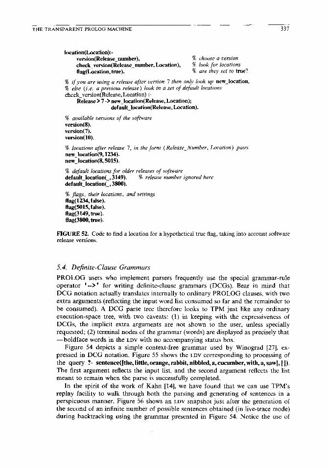
THE TRANSPARENT PROLOG MACHINE 337
location(Location):- version(Release_numher), % choose a version check_version(Releasnumher, Location), % look for locations flag(X.ocation, true). % are they set to true?
‘% if you are using a release after version 7 then only look up new-location, % else (i.e. a preview release) look in a set of default locations check_version(Release, Location) :-
Release > 7 -> new_location(Release, Location); default_location(Release, Location).
% available versions of the software version@). version(7). version( 10).
% locations after release 7, in the form (Release-Number, Location) pairs new_location(9,1234). new_location((l, 5015).
58 default locations for older releases of software default_location(_, 3149). % release number ignored here default_location(_, 3800).
% Jags, their locations, and settings flag( 1234, false). flag(5015,false). flag(3 149, true). flag(3800, true).
FIGURE 52. Code to find a location for a hypothetical true flag, taking into account software release versions.
5.4. Dejinite-Clause Grammars
PROLOG users who implement parsers frequently use the special grammar-rule operator ’ -->I for writing definite-clause grammars (DCGs). Bear in mind that DCG notation actually translates internally to ordinary PROLOG clauses, with two extra arguments (reflecting the input word list consumed so far and the remainder to be consumed). A DCG parse tree therefore looks to TPM just like any ordinary execution-space tree, with two caveats: (1) in keeping with the expressiveness of DCGs, the implicit extra arguments are not shown to the user, unless specially requested; (2) terminal nodes of the grammar (words) are displayed as precisely that -boldface words in the LDV with no accompanying status box.
Figure 54 depicts a simple context-free grammar used by Winograd [27], ex- pressed in DCG notation. Figure 55 shows the LDV corresponding to processing of the query ?- sentence([the, little, orange, rabbit, nibbled, a, cucumber, with, a, saw], [ I). The first argument reflects the input list, and the second argument reflects the list meant to remain when the parse is successfully completed.
In the spirit of the work of Kahn [14], we have found that we can use TPM’s replay facility to walk through both the parsing and generating of sentences in a perspicuous manner. Figure 56 shows an LDV snapshot just after the generation of the second of an infinite number of possible sentences obtained (in live-trace mode) during backtracking using the grammar presented in Figure 54. Notice the use of

33% MARC EISENSTADT AND MIKE BRAYSHAW
FIGURE 53. LDV for execution of ?- location(x), given the code shown iu Figure 52: (a) Snapshot at first invocation of the flag goal. (b) Final snapshot.
the strikethrough notation to indicate “succeeded earlier but failed upon backtrack- ing” for terminal nodes of the grammar, ie. words.
6. CONCLUSIONS
Our aim has been to reconcile a global view of PROLOG program execution with the truth about unification and clause selection. Moreover, we have wanted to satisfy both the needs of novices learning PROLOG and the needs of expert PROLOG users writing and debugging very large programs. These intentions have,

THETRANSPARENTPROLOGMACHINE 339
sentence --> np, vp. np --> det, np2. np --> np2.
np2 -4 noun. np2 --> adj, np2. np2 --> np2, pp.
pp 4 prep, np.
vp --> verb. vp --> verb, np. vp -3 verb, pp.
verb--> [nibbled]. verb --> [sings]. verb --> [saw].
noun --> [rabbit]. noun --> [cucumber]. noun --> [saw].
det --> [the]. det --> [a].
adj --> [orange]. adj --> Ilittle].
prep --> [with].
FIGURE 54. A simple context-free grammar expressed in DCG notation. The example is taken from [27, pp. 1971.
in turn, led us along a pathway of “creative tension” to satisfy somewhat contradic- tory constraints. The key ingredients of our approach have been (1) appreciation of the power of gestalt patterns, (2) recognition of the need (and the ability) to display thousands of nodes at a time, (3) enhancement of traditional AND/OR tree branches with individual clause details, (4) enhancement of AND/OR tree nodes with goal status boxes, and (5) ability to vary the type of detail being investigated with the particular grain size, rather than using a physical zoom.
Our work has developed from both ends simultaneously. That is, we were developing video-based teaching material for novice PROLOG programmers at the same time as we were implementing graphics facilities for observing a 2- or 3-thousand-node search space. Only by forcing these two paths to converge could we cater for the “upwardly mobile student” who learned about PROLOG in the early phases and then went on to become a serious PROLOG programmer.
TPM lends itself immediately to visual representation of parallel logic programs. In particular, the LDV diagrams should prove to be useful for monitoring the simultaneous execution of hundreds, or even thousands, of subgoals. Debugging of large parallel programs can be extremely difficult, and our intention is to expand our representation to cope with problems of both real-time and retrospective display of parallel execution.
An important motivating factor in all of our work has been the desire to build a system that we were happy to use ourselves. Toward this end, we are now using

340 MARC EISENSTADT AND MIKE BRAYSHAW
_sentence
the
&10un #yep
T T A,* rabbit cucumber with u u
"0"" a I
saw
FIGURE 55. Parse tree for the deliberately anomalous sentence [the, little, bled, a, cucumber, with, a, saw].
orange, rabbit, nib-
n sentence
FIGURE 56. Snapshot during the generation of multiple sentences using the grammar pre- sented in Figure 54.
+iiM+A- sings
rabbit
THE TRANSPARENT PROLOG MACHINE 341
TPM as part of our regular work, and are in the midst of a project to make the facilities described herein available in a practical, portable, and high-speed PROLOG environment.
REFERENCES 1.
2.
3.
4.
5.
6.
7.
8.
9.
10.
11.
12.
13.
14.
15.
16.
17.
18.
19.
20.
Bundy, A., Pain, H., Bma, P., and Lynch, L., A Proposed Prolog Story, DA1 Research Paper 283, Dept. of Artificial Intelligence, Univ. of Edinburgh, 1986.
Bundy, A., Pain, H., Bma, P., and Lynch, L., Impurities and the Proposed Prolog story, DAI Research Paper Addendum, Dept. of Artificial Intelligence, Univ. of Edinburgh, 1986.
Byrd, L., Understanding the control flow of Prolog programs, in: S.-A. Tamlund (ed.), Proceedings of the 1980 Logic Programming Workshop, 1980, pp. 127-138.
Coelho, H., Cotta, J. C., and Pereira, L. M., How to Soive it with Prolog. Laboratbrio National de Enginharia Civil (Minestt%io da Habita@ e obras publicas), Lisbon, 1982.
Coombs, M. J., Hartley, R. T., and Stell, J. G., Debugging user conceptions of interpreta- tion processes, in: Proceedings of the Fifth National Conference on ArtiJicial Intelligence (AAAZ-86), Philadelphia, 1986.
Coombs, M. J. and Sell, J. G., A Model for Debugging Prolog by Symbolic Execution: The Separation of Specification and Procedure, Research Report MMIGR137, Dept. of Computer Science, Univ. of Strathclyde, 1985.
duBoulay, J. B. H., O’Shea, T., and Monk, J., The black box inside the glass box: Presenting computing concepts to novices, Internal. J. Man-Machine Stud. 14(3):237-249 (1981).
Dewar, A. D. and Cleary, J. G., Graphical display of complex information within a Prolog debugger, Internat. J. Man-Machine Stud. 25:503-521 (1986).
Eisenstadt, M., A user-friendly software environment for the novice programmer, Comm. ACM 26, No. 12 (1983).
Eisenstadt, M., A powerful Prolog trace package, in: Proceedings of the Sixth European Conference on Artificial Intelligence (ECAI-84), North-Holland, Amsterdam, 1984.
Eisenstadt, M., Retrospective zooming: A knowledge based tracing and debugging methodology for logic programming, in: Proceedings of the Ninth International Joint Conference on Artificial Intelligence (ZJCAZ-85), Morgan Kaufmann, Los Angeles, 1985.
Eisenstadt, M. (ed.), Intensive Prolog, Open University Press, Milton Keynes, U.K., 1988.
Francez, N., Goldenberg, S., Pinter, R. Y., Tiomkin, M., and Tsur, S., An environment for logic programming, in: ACM Workshop on Software Engineering Environments, 1985, pp. 179-190.
Kahn, K., A grammar kit for Prolog, in: M. Yazdani (ed.), New Horizons in Educational Computing, Ellis Horwood, Chichester, U.K., 1984.
Komorowski, H. J. and Omori, S., A model and an implementation of a logic program- ming environment, in: ACM Workshop on Software Engineering Environments, 1985, pp. 191-198.
Lloyd, J. W., Declarative Error Diagnosis, Technical Report 86/3, Dept. of Computer Science, Univ. of Melbourne, 1986.
Matsumoto, H., A Static Analysis of Prolog Programs, Programming Systems Group Note 24, AI Applications Inst., Univ. of Edinburgh, 1985.
Model, M., Monitoring System Behavior in a Complex Computational Environment, Technical Report No. CSL-79-1, Xerox Palo Alto Research Center, 1979.
Pain, H. and Bundy, A., What stories should we tell novice Prolog programmers, in: R. Hawley (ed.), Artificial Intelligence Programming Environments, Wiley, New York, 1987.
Pereira, L. M., Rational debugging in logic programming, in: Proceedings of the Third International Conference on Logic Programming, London, 1986.
342 MARC EISENSTADT AND MIKE BRAYSHAW
21.
22.
23.
24.
25.
26. 27.
28.
Plaisted, D. A., An efficient bug location algorithm, in: Proceedings of the Second International Conference on Logic Programming, UppsaIa, 1984, pp. 151-157. Plummer, D., Coda: An Extended Debugger for Prolog, AI TR 87-54, Artificial Intelh- gence Lab., Univ. of Texas at Austin, 1987. Rajan, T., APT: A Principled Design for an Animated View of Program Execution for Novice Programmers, Technical Report No. 19, Human Cognition Research Lab., The Open Univ., Milton Keynes, U.K., 1986. Reiss, S. P., Graphical program development with PECAN program development systems, ACM SIGPUN Notices No. 19, 5 (1984). Rich, C. and Waters, R. C. (eds.), Readings in ArtiJcial IntelIigence and Software Engineering, Morgan Kaufmamr, Los Angeles, 1986. Shapiro, E. Y., Algorithmic Program Debugging, MIT Press, 1982. Winograd, T., Language as a Cognitive Process. Volume 1: Syntax, Addison-Wesley, Reading, Mass., 1983. Winston, P. H., Artificial Intelligence, 1st ed., Addison-Wesley, Reading, Mass., 1977.