the turbulent boundary layer with suction or...
TRANSCRIPT

R. & M. No. 3387
MINISTRY OF AVIATION
AERONAUlICAL RESEARCH COUNCIL
REPORTS AND MEMORANDA
The Turbulent Boundary Layer with Suctionor Injection
By T. J. BLACK, B.Se., Whit.Sehol., Grad.R.Ae.S., andA. J. SARNECKI, lV1.A., Grad.R .Ae. S.
OF CAMBRIDGE UNIVERSITY ENGINEERING DEPARTMENT
LONDON: HER MAJESTY'S STATIONERY OFFICE
1965
PRICE £1 7s. 6d. NET

The Turbulent' Boundary Layer with Suctionor Injection
By T. J. BLACK, B.Sc., Whit.Schol., Grad.R.Ae.S., andA. J. SARNECKI, M.A., Grad.R.Ae.S.
OF CAMBRIDGE UNIVERSITY ENGINEERING DEPARTMENTt
Reports and Memoranda No. 3J87*,
October, 1958
Summary.
This report considers the turbulent boundary layer with distributed suction or injection applied normallythrough the surface. A bilogarithmic law of the wall is established analogous to the logarithmic law forimpervious surfaces. Coles' wake hypothesis is extended to the transpiration layer and verified experimentally.The wall boundary condition is discussed briefly and possible effects of surface irregularity are examined.Finally the overall picture of the turbulent transpiration layer is discussed. It is considered that this reportprovides an acceptable framework for the evolution of a complete theory.
LIST OF CONTENTSSection
1. Introduction
2. The Turbulent Wall Region
2.1 Examination of existing theories
2.1.1 Examination of Kay's theory
2.1.2 Examination of the theory of Clarke, Menkes and Libby
2.1.3 Examination of Rubesin's theory and Mickley and Davis' analysis
2.2 Mixing-length theories with linearly varying mixing length applied to
constant-pressure boundary layers on continuously permeable walls
2.2.1 Equation of motion: velocity-shear relationship
2.2.2 Vorticity transfer theory with L = Ky
2.2.3 Momentum transfer theory with L = KY: bilogarithmic law
* Replaces A.R.C. 20 SOL
t Dr. Black is now at the Illinois Institute of Technology (Research Institute) Chicago; Dr. Sarnecki is atthe Royal Aircraft Establishment, Farnborough.

LIST OF CONTENTS-continuedSection
2.3 Application of bilogarithrnic law2.3.1 Methods of plotting2.3.2 The coefficients K and ,\
2.4 Experimental verification of bilogarithmic law2.4.1 Experimental data2.4.2 Analysis of velocity profiles obtained with suction2.4.3 Analysis of velocity profiles obtained with injection2.4.4 Summary of experimental results
3. Coles' Wake Hypothesis applied to Turbulent Boundary Layers with Transpiration
3.1 Introduction
3.2 Velocity-defect law
3.3 Coles' wake hypothesis
3.4 Experimental verification of Coles' wake hypothesis for transpiration layers
3.5 Summary
4. The Wall Boundary Condition in Two-dimensional Flow
4.1 The sublayer and blending region
4.2 The transition point
4.3 Transition criteria
5. Effects of Roughness and Non-Homogeneity of the Wall Surface
6. General Discussion of the Turbulent Boundary Layer with Transpiration
6.1 The basic mechanisms: inner and outer regions
6.2 Types of flow
6.3 Development of the layer
6.4 Effects of roughness and non-homogeneity of surface
7. Conclusions
Notation
List of References
Appendices I to III
Illustrations-Figs. 1 to 19
Detachable Abstract Cards
1. Introduction.
Since Prandtl's original work in 1904, a large amount of investigation has been conducted
concerning the problem of the boundary layer. Most of this work has been devoted to the case offlow over a solid surface. More recently, interest has been shown in the application of suction or
injection through the surface, the former to maintain laminar flow or to prevent separation, the
latter to provide surface cooling on the wings of high-speed aircraft or on turbine blades. The sucked
2

laminar layer in particular has been thoroughly investigated both theoretically and experimentally.
The turbulent layer with transpiration, however, is much less amenable to mathematical treatmentand little progress appears to have been made towards its solution. Moreover there is a lack ofsystematic experimental data which would permit the extension of existing semi-empirical theories
to include the effect of transpiration.Recently a thorough investigation of the turbulent boundary layer with transpiration has been
undertaken by the Engineering Department of Cambridge University. Some results have beenpublished by Kay! and Dutton", both of whom have demonstrated the existence of an 'asymptoticlayer' (of constant thickness) with uniformly distributed suction. Kay has put forward a tentativeanalysis for the asymptotic layer, but this could not readily be extended to the general sucked layer,whilst it is open to theoretical objections (Section 2.1.1).
Elsewhere an attempt to provide a theory for the turbulent layer with transpiration has beenmade by Clarke et al", but the neglect of an important relationship between certain parameters inthis analysis resulted in a high degree of disagreement between the predicted and actual velocityprofiles. Rubesirr' has developed a theory for compressible layers with injection, but has notconsidered the velocity distribution in detail nor has he considered the special case of incompressibleflow. Mickley and Davis" derived an incompressible form of Rubesin's analysis for comparison withtheir experimental velocity profiles, but did not develop the theory in detail, so that to date there is alack of a complete theoretical framework into which the observed behaviour of turbulent transpiration
layers may be fitted.The purpose of this report is to present such a framework for incompressible layers at least in zero
pressure gradient. Accordingly the report deals with the following:
(1) the existence of a law of the wall,
(2) the velocity distribution in the outer turbulent region,
(3) the conditions between the largely viscous sublayer and the fully turbulent region,
(4) the effects of different types of surface,
(5) the growth of the whole boundary layer with transpiration.
The law of the wall analogous to the logarithmic law for solid (impervious) surfaces is found tocontain a squared-logarithmic term and this prediction is borne out well by the measured velocityprofiles considered. In the outer region a velocity distribution corresponding to Coles." wake law isobserved. The situation is less satisfactory regarding the behaviour of the flow very near the wall.No reliable experimental data are available as measurements in this region are made extremelydifficult by the small thickness of the sublayer. Consequently the theoretical predictions for the flowin this region can only be tested indirectly, via the values of certain parameters in the law of thewall (corresponding to the constant term in the logarithmic solid-surface law). This is particularlytrue of the wall region in the boundary layer on a non-homogeneous permeable wall, since the flowin it exhibits not only turbulence (time-variation) but also spatial fluctuations which cannot bemeasured directly by any method available at present, due to the small length-scale of thefluctuations. Similarly the ideas presented on the growth and development of the turbulent layerwith transpiration are based more on intuitive reasoning than on the scanty experimental evidence.
The report is the result of many discussions between the authors, who have been investigatingdifferent aspects of the sucked turbulent layer and who had found the absence of a theoreticalfoundation a serious obstacle in their work.
3(90747) A2

2. The Turbulent Wall Region.
2.1. Examination of Existing Theories.
2.1.1. Examination of Kay's theory.-Kayl analyses only the asymptotic layer (i.e. one in
which the flow quantities do not vary with x). He assumes a mixing length proportional to distance
from the wallL = KY, (2.1.1)
and combines this with (i) the vorticity transfer theory (of G. 1. Taylor) and (ii) the momentum
transfer theory (of Prandtl) obtaining in the two cases:
(i)
(ii)
The equation of motion,
2 2 du d2u
K y---dy dy 2 '
(2.1.2)
(2.1.3)
(2.1.4)
(2.1.5)
u ~~ + v.~ = : G; -~~) ,reduces, for the asymptotic layer, to
du 1 d-rv o----- = - ---- ,
dy p dy
since dpldx = (iulax = 2vl2y = 0, so that v = vo, the normal velocity at the wall. (vo is negativesince suction is being applied.) Hence by substituting either equation (2.1.2) or (2.1.3) in (2.1.5)
and assuming
or
(i)
(ii)
duthat -- -> 0 as y -7 00 ,
dy
duthat u -> U1 as --- -7 0
dy ,
u
Kay obtains the following results:
(i)
(ii)
1 v (Y)'1 - - --() In -UI K 2 VI 8'
;;~ = 1 + 4b ~I In2 (~) .
(2.1.6)
(2.1.7)
Of these formulae equation (2.1.7) is shown to disagree with experimental results, whilst (2.1.6)
shows satisfactory agreement with Kay's results, which give a reasonably linear plot in the graph of
(1- u1U1 ) against In (yI8). Sarnecki's measurements in a layer which is very close to asymptoticconditions do not confirm this linear-logarithmic formula. It must be pointed out that Kay's
assumption duldy-+ 0 as y -r 00 (used to eliminate one of the constants of integration) is unsound
when applied to his formula, since he considers a boundary condition well outside the range of
application of his theory, for, as y -r 00, equation (2.1.6) gives u -700 and the value of its derivativeat that limit is insignificant.
Also, in the derivation of equation (2.1.7) Kay assumes that the relationship L = KY, (2.1.1),
holds throughout the thickness of the boundary layer which makes an unnecessarily restrictive
4

hypothesis as will be shown below. It will also be shown that Kay's analysis is restricted to thespecial case of asymptotic conditions which, as has been demonstrated by Dutton", is not as readilyattainable in turbulent as in laminar boundary layers with suction. The formulae (2.1.6) and (2.1.7)
cannot hold for non-asymptotic conditions, in particular at low values of suction, since as - V o ---+ 0they both yield u]U1 = const., whatever the behaviour of b. {The mixing-length coefficient K cannot
vanish, as can be seen from equations (2.1.2), (2.1.3).}
2.1.2. Examination of the theory of Clarke, Menkes and Libby.-Clarke, Menkes and Libby"
consider the general turbulent boundary layer with constant pressure on a permeable wall and point
out that in the neighbourhood of the wall the term Vo dU/dy is very much larger than UdU/OX {or(v-vo) dU/dy} and so the boundary-layer equation (2.1.4) reduces to a form identical with (2.1.5)
ou 1 07'Vo - =- -. (2.1.8)
oy P oy
They use the assumption of the momentum transfer theory, (2.1.3) and obtain (with slightlydifferent notation)
Vo OU = K 2~ [y2 (~U)2J .oy oy oy
Integration of equation (2.1.9) yields the result
U _ A B I (. UTY) 1 Vo I 2 (UTy)-- + n -- +~-n --U r V 4K 2 U r ,v .
(2.1.9)
(2.1.10)
Clarke et al use the equation (2.1.10) in that form, i.e. with two arbitrary constants {as demanded by(2.1.9) which is of second order}. They point out that for Vo -> 0 the equation (2.1.10) reduces tothe form
-. = A + Bin (UrY)TT 'U r V
(2.1.11)
(2.1.12)
the accepted logarithmic law for solid flat plates. In the absence of experimental data for the boundarylayer with suction or blowing they accept the solid plate values for A, Band K in their analysis ofexperimental profiles with injection and obtain poor agreement. Although Clarke et al recognise that
A, Band K should in general depend on volUc , they apparently overlook the relationship betweenthem which is implicit in the theory, as shown below.
2.1.3. Examination of Rubesin's theory and Mickley and Davis' analysis,-Rubesin4 dealswith compressible flow and obtains the velocity distributions in the sublayer and in the turbulentregion near the wall. His basic assumptions are, once again, the predominance of the V o au/oy termin equation (2.1.4) and the momentum transfer theory with linear mixing length, (2.1.1), (2.1.3).The two laws (sublayer and turbulent) are accepted as holding on either side of a transition point(y = Ya), at which the velocities and shear stresses {fL ou/oy and pI(2y2 (ou/oy)2 in the two cases}are matched. These assumptions lead to the following (u, y) relationships:
fu uduSublayer (0 < y < Ya) :y = ,
o PoVoU + TO
fu Kp'l2duTurbulent region (y > Ya):y = Ya exp V '
U a Povou + TO
with Ya to be determined empirically.
5
(2.1.13)

The integrations are carried out by Mickley and Davis" for the incompressible layer, (i.e. with
Po = P, f.L = vp, constants, and writing TO = pU,2). They obtain the following formulae:
U y U y U [( v u) 1/2 ( V U )1/2JTurbulent region: In .-", - In r :r a = 2K r 1 +?2, - 1 +~~' .V V V o , C, U, '
(2.1.14)
(2.1.15)
(2.2.1)
Mickley and Davis use this form of the equation in their comparison of theory with experiment,
plotting y logarithmically against (1 +VOU/U,2)lh and obtaining fairly good agreement with straight
lines of the predicted slope 2KfI,/vu for the turbulent region with U, obtained from momentum
considerations.This treatment is unduly restrictive, for whereas a linear graph may in general be used to determine
two unknown quantities (via the slope and intercept), here only the inner boundary condition (y(( or
equivalently u(() can be deduced from the experimental line, since the slope is predetermined.
Admittedly any variations in slope can be interpreted as variations in the mixing coefficient K, but
there are good grounds for assuming K to be a universal constant in two-dimensional flows, even
though some disagreement may exist as to its actual value. (See Appendix 1.)
The method developed in this paper is also based on a mixing-length analysis, but leads to a
different linear plot of velocity distributions which allows both the inner boundary condition and the
local skin friction to be determined from the velocity profile.
2.2. Mixing-Length Theories with Linearly Varying Mixing Length Applied to Constant-Pressure
Boundary Layers on Continuously Permeable Walls.
2.2.1. Equation (:f Motion: velocity-shear relationship.--The boundary layer underconsideration is taken to be incompressible, two-dimensional and obeying Prandtl's equation:
u au + v ru = 1 (aT _dP)ox oy p ry dx,'
and the continuity equation:
with the shear
ou ov·+--=0ox 3y
(2.2.2)
u = 0, v = V n at y = G.The condition at the boundary is
T
pau / ,» ')v,," - \U V .oy
(2.2.3)
(2.2.4)
(2.2.5)
Vn is greater than zero in the case of injection, less than zero for suction.
Sufficiently close to the wall ru/oy i8 large compared with u, ou/rx and (v - vn) [ = - f~ (iu/ax dyJ'so that the momentum transport u ru/rx + v ru/(iy is very nearly equal to V n (lu/(:y, and in theabsence of a pressure gradient the equation of motion (2.2.1) takes the form
au 1 aT'Vo _.- = - -;;..,,--- .
oy p oy
6

This equation is the exact analogue of the wall region assumption
o _! (17-pay' (2.2.5a)
for layers on impervious walls.
Equation (2.2.5) becomes accurate in a larger portion of the boundary layer as Iou/exl/I ou/oYIdecreases, and becom.es exact throughout the asymptotic layer. Moreover in all cases it is most
accurate in the immediate vicinity of the wall, where Iou/oy I is largest and lui, lou/oxl and Iv - volare smallest. In particular it holds well in the laminar sublayer.
Integration of equation (2.2.5) yields the velocity-shear relationship for the vicinity of the wall
On substituting
equation (2.2.6) becomes
T - TOvoU = '--.
p
TO
p
U 2T
r + VOU = -.p
(2.2.6)
(2.2.7)
(2.2.8)
This equation holds both in the laminar and in the turbulent portions of the wall region and
provides the justification for the simultaneous matching of u and Tat Y = Ya in Rubesin's analysis.The direct integration of equations (2.2.1), (2.2.2) through the boundary layer leads to the
momentum integral equation for layers with transpiration:
d (TT 20) dU 1 U <;O'il' TO U-d- u1 + ~d- 1° = --- + V o l'X X P
(2.2.9)
This equation holds generally for all two-dimensional layers without slip at the boundary. For layerswith constant pressure (dU 1/dx = 0), the equation takes the simple form
U 2 dO _ U 2 U1 dx - T + V o l' (2.2.9a)
2.2.2. Vorticity transfer theory with L = Ky.-The assumption of the vorticity transfertheory is that
(2.2.10)
Equation (2.2.10) can be substituted in (2.2.5), yielding a second-order differential equation:
i.e.02U V ooy2 = K2y2'
7
(2.2.11)

Integrating (2.2.11) twice:V ou = a + by - -2 In y .K
Defining 8 as the value of y at which equation (2.2.12) gives u = U1 ,
U1 = a + ss - ~~ In 8,K
so that
Vo Yu - U1 = b(y - 8) - ;;2 InS'
u = U1 + b(y - 8) - ~~ In ~.
(2.2.12)
(2.2.13)
In equation (2.2.13) band 8 are the constants of integration. One of them may be eliminated byapplying a suitable boundary condition in the region where (2.2.13) applies. Thus if the law is
assumed to hold throughout the layer, i.e. even at y = 8, the requisite condition may be taken as
au-- = 0 at y = 8.ay
Then
Vo V o- ;;28 + b = 0, b = ~28' and so
u = U1 - ;~ (In ~ + 1 - ~) . (2.2.14)
However even this condition cannot be applied with confidence in view of the common occurrence,
in the outer part of the turbulent boundary layer, of a 'tail' which departs from any law holding in
the inner region. Equation (2.2.14) can therefore only be applied to a layer without such a tail.
When comparing the predictions of vorticity transfer theory with experimental results, the
general form (2.2.13) must be used. It should however be noted that (2.2.13) can be written in the
form
(2.2.13a)
and for impervious walls (v o = 0) this reduces to u = const. + by, i.e. a linear velocity profile,which would contradict the well established logarithmic law, so that equation (2.2.13) cannot be
accepted for the whole range of v o, though it might give good results for some special cases such as
the asymptotic layer. Thus vorticity transfer theory with linearly varying mixing length is inadequate
for the description of a general boundary layer with suction or injection.
2.2.3. Momentum transfer theory with L = Ky: bilogarithmic law.-The assumption of the
momentum transfer theory is that
T
p2 2 (aU)2Ky -
Oy,
8
(2.2.15)

(2.2.16)
(2.2.17)
(2.2.18)
This can be substituted directly into (2.2.8) yielding a first-order differential equation:
(OU) 2 = (_K)' 2 (O[Ur
2+ VOU])2,U 2 + VOU = K2y2 -r oy V o alny .
which integrates to V(Ur2 + VOU) = (VO/2K) In (y/d) with d as the one constant of integration,i.e.
Ur 2 + VoU = (;; In~r
This is the basic form of the law of the wall with transpiration under the assumptions of momentumtransfer theory with linear variation of mixing length. It will be referred to as the bilogarithmic law.
From equation (2.2.17)au V 0
2 2 yVo ay = 4K2 YIn {j'
au Vo yoy = 2K2y In {j'
Now ou/oy > 0 throughout the region of validity of equation (2.2.17). Therefore for a suckedlayer, Vo < 0, In (y/d) < 0, y < d and d is of the order of the total boundary-layer thickness. Withinjection, Vo > 0, In (y/d) > 0, Y > d and d is of the order of the sub layer thickness. With suction,the velocity predicted by equation (2.2.17) has a maximum at y = d whilst with injection the graphof u has a minimum at y = d. In neither case however can the bilogarithmic law hold at the point,since the basic assumption that the turbulent shear is much larger than the viscous shear breaksdown. For
ou V o YT vise = ev -;:;- = pv 2~ In -d'oy Ky
(OU) 2 V 2 ( Y)2
Tturb = pK2y2 2y = p 4:2 In d '
:tu':!' = ! vo~ In ~ -?- 0, as y -?- d.Tvise 2 v d
2.3. Application of the Bilogarithmic Law.
(2.2.19)
(2.2.20)
(2.2.21)
(2.3.1)
2.3.1. Methods ofplotting.-The bilogarithmic law obtained in Section 2.2.3
U r 2 + vou = (~: ln~) 2
can be expected to hold in the inner turbulent region of all boundary layers with continuouslydistributed suction or injection, provided that
(i) the flow is nearly two-dimensional
(ii) the pressure gradient normal to the surface is negligible, i.e. Prandtl's equation holds
(iii) the laminar sublayer does not occupy a very large proportion of the boundary-layer thickness,i.e. the region in which equation (2.2.8) holds is not completely laminar.
9

In particular a suitable limiting form of (2.3.1) holds in the case of impervious boundaries, V o = O.Equation (2.3.1) can be rewritten in any of the following forms
(i)
(ii)
t.e.
u(2.3.2)
with
(2.3.3)
where
aIt.
b = -,K
(2.3.4)
(iii)
i.e.
(2.3.5)
Equation (2.3.2) provides a universal method of plotting experimental results for comparison with
theory, for when a layer satisfying the bilogarithmic law is plotted on the basis of ujvo against
logy, the resultant graph must be a parabola of fixed shape (for a given value of K), with its axis
along increasing llj7)o and its apex at y = d, Uj7Jo = - UT2j7'o2. Thus a single standard curve would
in theory be sufficient to determine both UT and the value of d for an experimental velocity profile,by sliding the theoretical curve over the experimental graph until a good fit is obtained. In practicethis method fails because of the large range of values of ujvo encountered and the small curvature
of the standard parabola, leading to a high degree of uncertainty over the exact location of theall-important apex.
Equations (2.3.3) to (2.3.5) present the form of the bilogarithmic law analogous to the orthodoxlogarithmic law for boundary layers on impervious boundaries
with
U = A + B In ~UTYUT V
1B = .~.
K
(2.3.3a)
(2.3.4a)
The most convenient method of plotting experimental results is in the form suggested by equation
(2.3.6) since the left-hand side of the equation contains only quantities which are measurable directly
(the value of K is assumed known), and the right-hand side is linear in log (U1yjv). In practice the
best way of using equation (2.3.6) is to use not logy but a suitable multiple of it as the abscissa,
as follows:
10

In the case of suction (vo < 0), use the substitution
(2.3.8)
then equation (2.3.6) reduces to
(2.3.9)
with
(2.3.10)
and
With injection (vo > 0) the substitution
~ J(Vo) In V 1Y = y.2K V1
V . t'
leads to
with
and
(2.3.11)
(2.3.12)
(2.3.13)
(2.3.14)
(2.3.15)
The advantage of using Y rather than log (V1y lv) lies in the fact that in the graph of u] V 1 ± Y2against Y the curves of zero velocity and full free-stream velocity (u = 0, u = Vi) are then fixedparabolae (u1V1 + Y s2 = Y s2 , 1+ Y s2 for all sucked layers; u1V1 - Y i 2 = - Yi 2 , 1- Yi 2 for all blownlayers) independent of the actual value of vol V 1 , so that direct comparison may be made betweenlayers with different rates of suction or of injection, and the state of the boundary layer can bededuced from the geometry of the system of the two parabolae and the experimental straight line.Thus in the case of suction the straight line will cut, touch or not cut the parabola u] V 1 = 1according as Ps2 is greater than, equal to, or less than unity; similarly in the case of injection the straightline will cut, touch or not cut the parabola u] V 1 = 0 according as Pi2 is greater than, equal to, orless than zero.
The momentum integral equation with transpiration in zero pressure gradient takes the form(2.2.9a):
V 12 dB = T T 2 V
dx G T + V o l'
or
(2.3.16)
11

Thus with suction [from equation (2.3.11)]
(2.3.17)
and the boundary layer is growing if p} > 1 (experimental straight line cuts the parabola u] UI = 1).
Such a layer can be termed undersucked.
Ifp,2 = 1 (line touches parabola), the boundary layer has constant (momentum) thickness and so
has reached the asymptotic condition.
If p,2 < 1 (line does not meet parabola), the momentum thickness is actually decreasing and the
layer will be called oversucked.
With injection (2.3.15)
de vdxU(Pi2+1). (2.3.18)
I
Thus with injection the boundary layer always grows and, as a rule, dejdx ;0, vojVI' if the assump
tions of the basic theory hold (two-dimensional flow, no slip). The experimental straight line then
cuts the parabola uj U I = O. It is tangential to it when the effective wall shear vanishes (i.e. Pi2 = 0).This condition need not imply separation and it is shown in Section 5 that both zero and negative
effective wall shear may be encountered in an unseparated layer. In the latter case the straightline fails to meet the parabola.
Typical profiles plotted as (ujl\ + Y" uj VI - Yi ) against Y" Y i are shown in Fig. la (suction)and Fig. 1b (injection). Fig. 1c shows profiles, with V o less than, equal to and greater than zero,
plotted on the more familiar basis of ul U; against log VTyjv to show the curvature of the
'bilogarithmic' profiles.
The relationship between the parameter ,\ defined by equation (2.3.5) and the constants
determined from the linear plot is as follows. For suction
For injection
(2.3.19)
(2.3.20)
If U T2 (and p?) vanish, then the boundary layer cannot be plotted as ujUT against log UTY/v.
If U T2 (and Pi2
) are negative, then U T is imaginary but finite and the velocity profile can be plotted
in the form uli.U ; against log (iUTyjv), (i = vi -1). Equation (2.3.3) can then be rewritten
with
(2.3.21)
where
It.'b' =
K(2.3.22)
(2.3.23)
The physical significance of the imaginary U; (negative wall shear) will be discussed in Section 5.
12

2.3.2. The coefficients K and A.-The bilogarithmic law for the turbulent boundary layer,when expressed in the form analogous to the universal law for solid boundaries, equations (2.3.3 to2.3.5), contains two dimensionless coefficients, K and A. The only condition imposed on these by thebasic theory is that they should be independent of wall distance y. They can vary with vo, UT andtype of surface employed, but in such a way that, for a smooth surface, when V o = athe coefficientsa {= (UT IVo)(A2- 1)}and b(= AI K) reduce to their universal solid-case values A and B (seeAppendix I).
It can be argued intuitively that the mixing-length coefficient should be independent of thetranspiration velocity vo, provided V o is small by comparison with the longitudinal velocity in theregion where the assumptions of the mixing-length theory hold. For if a slice of a mean-flowstream-tube is taken as a control volume, the mixing length in it can be described as KY' where K maydepend on the local curvature of the flow, and the effective wall distance y' may not be identical withy. If however v is small in the control volume, then the inclination of the stream to the wall isnegligibly small, and the curvature even more so. In practice v is rarely greater than 0·01 UI and
u does not fall below 0·25 U1 in the turbulent region so that v [u < O'04 and the inclination
ex < O·04 radians: thus y' (which might be expected to depart from y to the same extent as cos ex
departs from 1) does not differ from y by more than O' 1%. The curvature might be important if theratio of wall distance to the radius of curvature became appreciable. However this ratio
~ y(vlu) oex!oy, which is of even smaller order of magnitude than ex, so that for the small values of Voapplied in practice these considerations suggest that the turbulence in the flow is unaffected by the
crossflow v. Hence there appears no reason why K should change with Vo from its universal solidwall value, and if the model of a turbulent boundary layer described by mixing-length theory withL = Ky is acceptable for solid boundaries, the condition of transpiration can be included withoutmaking the model any less accurate and with the value of K unchanged. The solid-plate value ofK = 1/B (see Appendix I) will therefore be used in all calculations.
The profile parameter A, defined by equation (2.3.5) is essentially a constant of integration andso must be related to a boundary condition. It is in fact determined by the way in which the viscouslaw of the sublayer blends with the bilogarithmic law of the fully turbulent region. The laws governingthe flow in this blending region are as yet uncertain. The mere superposition of viscous effects andthe turbulent stresses derived from the momentum transfer theory with L = Ky, fails to predict thebehaviour of the flow when Vo = 0, and as shown by Van Driest? a damping factor has to beintroduced. Van Driest's analysis can be extended to include transpiration but a large amount ofnumerical computation is involved and the results are pot yet available, though it is hoped topublish them later. An approximate method of predicting the variation of Awith suction or injectionis described in Section 4.
2.4. Experimental Verification of Bilogarithmic Law.
2.4.1. Experimental data.-There exists only a limited amount of experimental data onthe velocity distribution in the turbulent boundary layer with suction or injection applied normallythrough the surface. Some of the available velocity profiles are based on only a few experimental
points and therefore cannot provide a conclusive test for any theory, but are included in the presentreport for completeness.
Twenty-four velocity profiles have been examined, sixteen obtained with suction and eight
with injection. All these measurements were obtained with zero pressure gradient, and cover a widerange of suction and injection velocity ratios, as shown in Table 2.4.1.
13
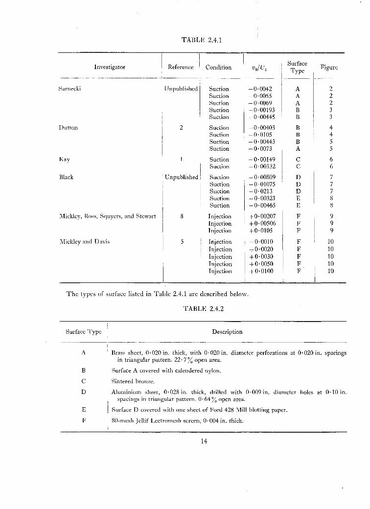
TABLE 2.4.1
SuctionSuction
, Unpublished SuctionSuctionSuctionSuctionSuction
8 InjectionInjectionInjection
5 InjectionInjectionInjectionInjectionInjection
22233
4455
66
77788
999
1010101010
Figure
AAABB
BBBA
CC
DDDEE
FFF
FFFFF
SurfaceType
-0'0042-0,0055-0,0069-0·00193-0·00445
-0'00403-0·0105-0,00443-0·0073
-0,00149-0,00332
-0·00809-0·01075-0,0213-0,00321-0,00465
+0·00207+0·00506+0·0105
+0·0010+0·0020+0·0030+0·0050+0·0100
SuctionSuctionSuctionSuction
2
I
R f i e die erence i .on rtion
I 1--------..
I
I Unpublished I' SuctionSuctionSuction
I i SuctionI Suctioni
I
I
Mickley and Davis
Investigator
Black
Mickley, Ross, Squyers, and Stewart
Kay
Dutton
Sarnecki
The types of surface listed in Table 2.4.1 are described below.
TABLE 2.4.2
ISurface Type I Description
-------~---I---···_--------~-A . Brass sheet, 0·020 in. thick, with 0·020 in. diameter perforations at 0·020 in. spacings
in triangular pattern. 22·7 %open area.
B Surface A covered with calendered nylon.
C Sintered bronze.
D Aluminium sheet, 0·028 in. thick, drilled with 0·009 in. diameter holes at 0·10 in.spacings in triangular pattern. 0·64 %open area.
E Surface D covered with one sheet of Ford 428 Mill blotting paper.
F 80-mesh Jellif Lectromesh screen, 0·004 in. thick.
14

2.4.2. Analysis of velocity profiles obtained with suction.-In Figs. 2 to 8 inclusive, velocityprofiles obtained with suction are examined in the light of the bilogarithmic law. Fig. a in each caseshows a plot of ujU1 + Ys2 against Ys' and includes the authors' choice of straight line to fit thebilogarithmic portion of each profile. The slope and intercept of this straight line yields values ofUrjU1 and the profile parameter A [equations (2.3.11), (2.3.19)]. These values enable the profile to bereplotted in the familiar form ul U; against log Uryjv in Fig. b. This plot has been included to showthe curvature of the bilogarithmic portion of each profile, which cannot be satisfactorily accountedfor by a linear logarithmic law, particularly at high suction rates. Included in Fig. bare sublayer
profiles as predicted by equation (4.1.6). Figs. 2 to 8 will now be discussed in detail.Fig. 2 shows three profiles obtained at different suction rates on a perforated surface (type A)
by Sarnecki. Each of these profiles has a clearly defined linear portion in Fig. 2a, while the
pronounced curvature of this region in Fig. 2b shows that a linear logarithmic law cannot apply.
In Fig. 2a, the chosen straight lines in the case of the lower suction rates do not cut or touch the
parabola ujU1 = 1, indicating that the boundary-layer thickness is decreasing locally. For the highest
rate of suction, however, the boundary layer has already reached its asymptotic state at the stationconsidered as indicated by the fact that the chosen straight line is tangential to the parabolic curve.It is of interest to note that the bilogarithmic region in the latter case extends to the edge of theboundary layer. The absence of an 'outer' or 'wake' region appears to be a characteristic of the
turbulent asymptotic layer.Fig. 3 shows two profiles obtained by Sarnecki on a porous surface (type B). The bilogarithmic
law provides a good fit to the 'inner' portion of the profiles, although the curvature of this regionin Fig. 3b is not sufficient to argue positively in its favour. For the lower suction rate, the chosenstraight line in Fig. 3a cuts the parabola u] U1 = 1, indicating that the boundary-layer thickness isincreasing, i.e. that the layer is undersucked. The chosen straight line for the higher suction rate isalmost tangential to the curve indicating near-asymptotic conditions (again note the diminutivesize of the 'wake component').
Fig. 4 shows two profiles obtained by Dutton on the same type of surface (type B). Unfortunatelyvery few experimental points were obtained in each case. However, straight lines can be chosento fit the bilogarithmic portion in Fig. 4a, and the law provides a good interpretation of this regionas shown in Fig. 4b. It can be seen from Fig. 4a that the layers are respectively undersucked andoversucked for the lower and higher suction rates.
Fig. 5 shows the profiles of two asymptotic layers obtained by Dutton on surfaces A and B.In each case the suction rate was uniform and was adjusted until an asymptotic layer was obtainedover almost the complete test section. Again very few experimental points were recorded, and thechoice of straight lines in Fig. Sa, proved difficult. The selected straight lines are tangential to theparabola uj U1 = 1 indicating the asymptotic nature of the layers.
Dutton obtained values of Uri U1 from the asymptotic form of the momentum equation
(2.4.1 )
and plotted the profiles as ujUr against log Uryjv. He assumed Kay's linear logarithmic law[equation (2.1.6)], which has already been criticised on theoretical grounds, and drew straight linesthrough the experimental points. It may well be argued on examination of the experimental pointsin Fig. Sb that this interpretation provides as good a fit as the bilogarithmic law. However the values
15

(2.4.2)
of the mixing-length coefficient given by Kay's analysis are O· 35 and 0·31 for the perforated and
nylon surfaces (types A and B) respectively, and as it has already been argued that K should be
independent of the suction rate (Section 2.3.2), the bilogarithmic law appears more attractivein this case.
Fig. 6 shows two profiles obtained by Kay on a porous surface (type C). Owing to the relatively low
suction rates, the curvature of the bilogarithmic portion in Fig. 6b is only slight.
The profiles of Fig. 7 were obtained by Black on a drilled surface (type D), with relatively high
suction rates. They exhibit a marked degree of curvature in Fig. 7b, which is satisfactorily accounted
for by the bilogarithmic law.* It is particularly interesting that the law is found to be valid even in
the case of a non-homogeneous surface of extremely small open-area ratio (0· 65%). The complete
absence of a 'wake component' in each case is also worthy of note.
Fig. 8 shows profiles obtained by Black with the drilled sheet covered with a sheet of blotting
paper (surface type E). (The blotting paper was used to obtain a more nearly uniform distribution
of suction.)
The experimental velocity profiles examined above show satisfactory agreement with the proposed
bilogarithmic law, but the boundary-layer growth predicted from the profiles by the present theory
can only be checked in two cases apart from that of the asymptotic layers (for which the straight
lines are tangent to the parabola as required by the theory). This has been done for the measurements
made by Dutton at two suction rates. In each case velocity profiles were measured at close intervals
along the test surface, those in Fig. 4 being typical examples. These profiles have been examined by
the authors, using the bilogarithmic law to obtain values of UTIUi from which the growth of
momentum thickness has been calculated by means of the momentum equation
~~ = (~r + 'J~'The calculated and experimental growths of e are compared in Fig. 9. The remarkably good
agreement confirms the values of UTI Ui deduced using the bilogarithmic law. [It should be noted that
the two terms on the right-hand side of equation (2.4.2), which are of opposite sign in this case, were
of comparable magnitude, so that the measure of agreement obtained becomes even more satisfactory.]
2.4.3. Analysis of velocity profiles obtained with inJection.-In Figs. 10 and 11, velocity
profiles obtained with injection through a mesh surface by Mickley et al8• 5 are examined.
Mickley" measured velocity profiles at various stations along the test surface under conditions of
suction and injection, with and without heat transfer from the wall.']: It was subsequently discovered
that the heating cloth, initially attached to the back of the test surface for use in the heat transfer
experiments, became detached from it at some stage, permitting longitudinal flow beneath the
surface. It was stated by Mickley that, as a result, the reported skin-friction coefficients were likelyto be 15 to 30(;;) higher than the correct values, and that in general the results should not be used.
Presumably because of the absence of other experimental data, Clarke, Menkes and Libby" used
three of these profiles to compare with their analysis of the turbulent boundary layer with injection.
The agreement they obtained was poor however, particularly in the shape of the profiles, and it was
* The predicted sublayer profiles are included in this figure even though no agreement with the experimentalsublayer profiles can be expected in view of the highly non-homogeneous nature of the surface.
t The profiles included in this report were all obtained without heat transfer.
16

therefore considered of interest to analyse these profiles accordingto the present theory. The resultsare shown in Fig. 10. Fig. lOa contains a plot of uj U I - Y i 2 against Y i , from which values of
UTI UI and ,\ are obtained as in the case of suction. It will be noted that the chosen straight line forthe highest injection rate is tangential to the parabola u] UI = 0 indicating zero effective wall shear.This prevents the replotting of this profile in the conventional manner tu]UTagainst UTy/v). The othertwo profiles, however, are replotted in Fig. lOb, and the bilogarithmic law is seen to fit the
experimental points quite well.Mickley-Iater modified his experimental apparatus to eliminate the undesirable effects experienced
in his earlier work, and obtained velocity profiles at various stations for different injection rates.Typical profiles are examined in Fig. 11. In Fig. l l a the chosen straight lines for the two lower
injection rates cut the parabola u] UI = 0, indicating positive wall shear. For the intermediateinjection rate, (va! UI = 0,003) the straight line is almost tangential to the parabola, indicatingnegligible wall shear. For the two higher injection rates, the straight line lies outside the parabola,indicating negative effective wall shear. The first two profiles are replotted in the form, u] UT
against log UTYlv in Fig. l lb. The curvature of the bilogarithmic region is small in view of therelatively low injection rates. Again; the profile obtained with vol UI = O·003 cannot be replottedas UTIUI is negligibly small for this case. For the higher injection rates, UT!UI is imaginary. Thebilogarithmic law for imaginary UTI UI is given in equation (2.3.21) and the profiles may thereforebe replotted in the form ulill; against log iUTy!v, where i = V-I. Fig. l Ic shows the profilesplotted in this way. It will be seen that the profile for the highest injection rate displays a highdegree of curvature which the bilogarithmic law accounts for very satisfactorily.
Mickley calculated UT! UI from the momentum equation (2.4.2) and obtained negative values of(UTIUI)2for the two higher injection rates. As this required taking the small difference of two largequantities, one of which was obtained by differentiation of experimental results, Mickley statedthat these negative values were probably of no significance, adding that the measured velocityprofiles showed no evidence of separation. In Section 5 of this report the case of transpiration through
non-homogeneous surfaces is considered, and the conclusion drawn from this analysis is that negative
values of effective* wall shear may occur at high injection rates on surfaces where the hole dimensionsare appreciable. It is suggested that this provides the explanation of the negative values of wall
shear discussed above. It is important to note that negative effective wall shear in the present case(i.e. for high injection rates) does not imply negative u near the wall, nor even inflection of the velocityprofile] such as occurs near separation on a solid surface. There is, in fact, no reason at all to suspectthat the injected layer in zero pressure gradient will ever separate in that sense of the word whichimplies a general breakdown of the boundary-layer flow with associated 'dead-air' region andbackflow.
In Fig. 12, the growth of momentum thickness calculated for the five injection rates, usingvalues of UTI UI obtained from the bilogarithmic law, in conjunction with the momentum equation(2.4.2), is compared with the actual growth of () obtained experimentally by Mickley. The agreementis quite good. It must be noted, however, that the contribution of the injection term, va!UI , in
* Effective in the sense that these values satisfy the momentum equation (2.4.2) and the bilogarithmic law.
t Although velocity profiles obtained with high injection rates tend to be doubly reflex roughly midwaybetween the wall and the edge of the layer, this is a characteristic of the blown layer and is not in generalindicative of zero or negative wall shear.
17(90747) B

(3.2.1)
equation (2.4.2) is in each case substantially greater than that of (UTI U1)2 and any errors in thelatter quantity are therefore largely suppressed in Fig. 12. Average values of ( UTI U1)2 are listedfor each case in Fig. 12 to show the relative importance of the two terms.
Discussion of the experimental values of ,\ determined for the profiles considered in this report
will be postponed to Section 4.3.
2.4.4. Summary of experimental results.
(1) The bilogarithmic law adequately predicts the velocity distribution in the wall region outside
the sublayer, for the cases examined. In particular, profiles obtained with high transpiration rates
amply justify the squared-logarithmic term in the law.
(2) The values of [fTIU1 obtained from the bilogarithmic law satisfy the momentum equation
in the few cases where experimental data are available for comparison.
(3) The bilogarithmic law appears to be equally valid in cases of effectively negative wall shear
(imaginary lIT)'
3. Coles' Wake Hypothesis Applied to Turbulent Boundary Layers with Transpiration.
3.1. Introduction.
Having estahlished the existence of the hilogarithmic law in the inner region of the turbulent
boundary layer with transpiration, an attempt can now be made to analyse the outer region of thelayer. Stated briefly, the prohlem is one of determining, if possible, a universal law associated withthe velocity distribution in the outer region. Existing theories developed for the particular case ofzero transpiration are examined first, to determine whether they may be extended to include thegeneral case of suction or injection. Two approaches which have been made to the problem in thecase of no suction are considered helow.
3.2. Velocity-Defect Law.
It has been found for constant-pressure layers on a solid surface, that the velocity profiles lie
close to a single curve when plotted as (U 1 - u)/UT againstyl8 (see Fig. 3, Ref. 9).This relationship, expressed in the form
U~~ u = g (~),
is known as the velocity-defect law, and implies downstream similarity of the profile. By assuming
the existence of the defect law and of a law of the wall of the form
_u_ = f (!!TY) ,UT v
Millikan deduced the logarithmic law
u UTy= A + BIn ----
[IT v
(3.2.2)
(3.2.3)
as follows:
From (3.2.2)
while from the defect law
Y au = ~UvTf' (_UVTY) ,U
Tay
fJ~~;= _~gl(~).
18
(3.2.4)
(3.2.5)

The concept of overlap is now introduced. This presupposes a finite region in which the defect andwall laws are simultaneously valid. This requires
y oy
ii, oy
1K
(3.2.6)
Then K is determined by either of the variables y/8 or yUr/v, and since these two variables areformally independent of each other, K must be a constant.
On integrating (3.2.6) in the overlap region, the logarithmic law
= A + B log Ur y.v
(3.2.7)
is obtained.The above result states that the existence of a logarithmic law in the inner region is an essential
condition for the validity of the defect law with overlap.Examination of experimental velocity profiles obtained in pressure gradients has shown that the
function g(y/8) in equation (3.2.1) is not a universal function (see Fig. 18, Ref. 6). To include theeffects of pressure gradient, the velocity-defect law must be expressed in the more general forrr
U1 - u (y )U;- = g 8' IT(x) , (3.2.8)
where the profile parameter IT in general depends on the pressure gradient.An equilibrium layer has been defined as one for which IT is constant, the constant-pressure
layer being a particular example. Clauser? has succeeded in obtaining equilibrium layers in pressuregradients of a special form.
When consideration is given to the general case of layers with transpiration, it is obvious fromMillikan's analysis that a velocity-defect law (U1-u)/Ur = g(y/8, vo/Ur) cannot overlap thebilogarithmic law. The assumption of a defect law of this form would therefore require that theoverlap region be replaced by a blending region between the inner and outer portions of the layer.Such a requirement would complicate the physical picture unnecessarily and would not provide asound basis on which to construct a calculation method for the development of sucked or injectedlayers. The fact that the defect law is not universal for arbitrary pressure gradients provides furtherground for its rejection.
Consideration is now given to a more recent approach to the problem.
19(90747) B2
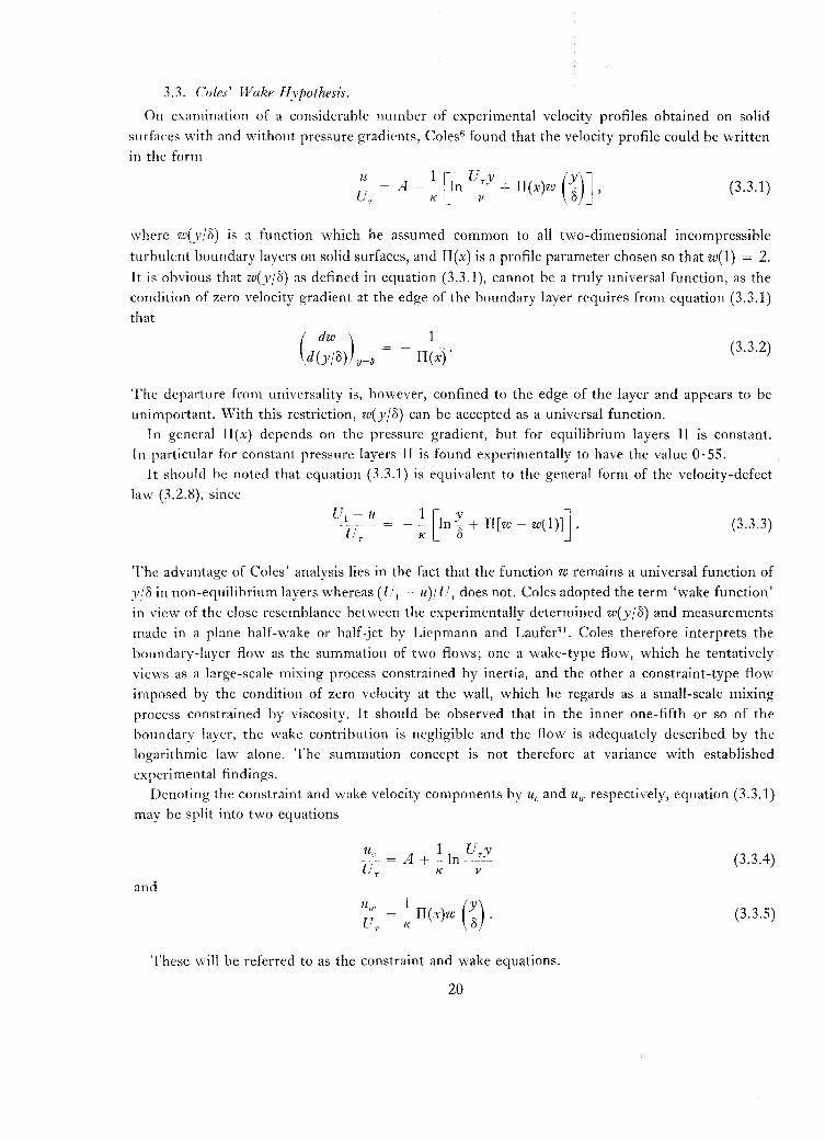
3.3. Cules' Wake Hyputhesis.
On examination of a considerable number of experimental velocity profiles obtained on solid
surfaces with and without pressure gradients, Coles" found that the velocity profile could be written
in the form
u 1[ UTy·· (Y)JUT
= f1 + K In v - + lI(x)w ;3 , (3.3.1)
where w(y/8) is a function which he assumed common to all two-dimensional incompressible
turhulent houndary layers on solid surfaces, and Tl(x) is a profile parameter chosen so that w(1) = 2.It is ohvious that w(y/8) as defined in equation (3.3.1), cannot be a truly universal function, as the
condition of zero velocity gradient at the edge of the boundary layer requires from equation (3.3.1)
that1
11 (x) . (3.3.2)
The departure from universality is, however, confined to the edge of the layer and appears to be
unimportant. With this restriction, w(yj8) can be accepted as a universal function.
In general Il (x) depends on the pressure gradient, but for equilibrium layers IT is constant.
In particular for constant pressure layers Il is found experimentally to have the value O·55.It should be noted that equation (3.3.1) is equivalent to the general form of the velocity-defect
law (3.2.8), since
U1 - u 1 [Y - Jti, = - ~ In 8 + lI[w - w(1)] . (3.3.3)
The advantage of Coles' analysis lies in the fact that the function w remains a universal function of
y /8 in non-equilibrium layers whereas (U1 - u)j U T does not. Coles adopted the term 'wake function'
in view of the close resemblance between the experimentally determined w(yj8) and measurements
made in a plane half-wake or half-jet by Liepmann and Laufer!'. Coles therefore interprets the
boundary-layer flow as the summation of two flows; one a wake-type flow, which he tentatively
views as a large-scale mixing process constrained by inertia, and the other a constraint-type flow
imposed by the condition of zero velocity at the wall, which he regards as a small-scale mixing
process constrained by viscosity. It should be observed that in the inner one-fifth or so of the
boundary layer, the wake contribution is negligible and the flow is adequately described by the
logarithmic law alone. The summation concept is not therefore at variance with established
experimental findings.
Denoting the constraint and wake velocity components by u" and u.; respectively, equation (3.3.1)
may be split into two equations
and
Uw 1 (Y)UT
= K n(x)w-8 .
These will be referred to as the constraint and wake equations.
20
(3.3.4)
(3.3.5)

The simplest extension of Coles' hypothesis to layers with suction or injection suggests thegeneral form of the constraint and wake equations to be
and
u; 1 ) (y)- = - II(x w - ,ti, K 0
(3.3.6)
(3.3.7)
where the bilogarithmic law replaces the solid-surface logarithmic law, and the wake equation
remains unaltered except in so far as II(x) may now be a function of the transpiration rate as well aspressure gradient. The validity of equation (3.3.7) can easily be checked experimentally.
It appears unrealistic, however, that the magnitude of the wake component Uw at every point inthe layer, should be determined by the friction velocity U; which represents an influence acting at
the wall (i.e. wall shear). On the other hand very convincing experimental evidence is presented
in Coles' report in favour of the wake law as stated in equation (3.3.5). This suggests the possibilityof replacing U; in equation (3.3.7) by a representative velocity which may in general be a function
of x and y, but which is a constant multiple of U; in the particular case of zero transpiration.One such velocity is the local constraint shear velocity u*e defined by
or from equation (3.3.6)
OUeu*e = Y -oy
= -~ v(u,2 + VOU e),K
(see Section 6.1)
(3.3.8)
U*c obviously satisfies the two requirements mentioned above; firstly it is a truly local property ofthe layer, i.e. a function of x and y, and secondly, for zero transpiration ("'0 = 0, A = 1) it is a constantmultiple of Ur •
On replacing U; by u*e equation (3.3.7) becomes
Uu' = II(x)w (2')
u*e 0(3.3.9)
which reduces to equation (3.3.5) for Vo = O.u*e increases with y for injection and decreases for suction, but the total variation in u*c across
the layer only becomes appreciable at relatively high transpiration rates. It remains, now, to test the
validity of equations (3.3.7) and (3.3.9) for the experimental profiles available.
3.4. Experimental Verification of Coles' Wake Hypothesis for Transpiration Layers.
Only six of the profiles obtained with suction together with the eight obtained with injection,possessed wake components of sufficient magnitude to permit analysis. In each case the wakecomponent velocity Uw was obtained by subtracting the constraint velocity Ue (as determined from the
21

bilogarithmic law) from the total velocity u. Equations (3.3.6) and (3.3.8) were then applied to
obtain n n W T (yjo) and n,X<, w* (yjo) respectively'[. °being determined by the maximum value ofuu.( U T or u",jtt'X<,.. W T and W* were then obtained by satisfying Coles' normalising condition w(l) = 2,
while II followed from the equations
and
liT (3.4.1)
(3.4.2)
WT
and W* are plotted for each of the profiles considered in sub-figures a and b of Figs. 14 to 18.Included in each figure is the wake function as tabulated by Coles.
Fig. 14 shows the functions WT
and w* obtained from two of the velocity profiles of Fig. 2.
The agreement between WT
and Coles' Wake Function is poor. The agreement for w*, although
considerably better, is still not of the standard obtained by Coles for the solid-surface data. The
profiles in question, however, were obtained in oversucked layers. In such layers the value of
u*, decreases rapidly with increasing y to approximately zero at the edge of the boundary layer, and
accurate determination of °and w(yjo) becomes exceedingly difficult.
The functions WT
and w~, for the suction profiles shown in Fig. 3 are plotted in Fig. 15. Agreement
with the Wake Function is fair for W T but good for w* within the experimental scatter.]
zc, and w* for the profiles of Fig. 8 are plotted in Fig. 16. Again the agreement, whilst only fair
for W n is good for w*.
In Figs. 17 and 18, W T and W * are plotted for the injection profiles of Figs. 9 and 10. Here again
the experimental evidence appears to be slightly in favour of 'w'X< which agrees well with the Wake
Function.
In each of Figs. 14 to 18, values of rr T and TI* are included. Both n T and IT * tend to decrease withincreasing suction, and increase with increasing injection, although this trend is not well defined.I n particular, imaginary values of n T are obtained for two of the injection cases in Fig. 18. These
values occur as a direct consequence of the non-homogeneity of the surface, which results in
negative effective wall shear (imaginary UT)' (See Section 5.) It is unlikely, however, that the flow
in the outer region should be directly affected by non-homogeneity of the surface, and it appearsunrealistic, therefore, that the wake parameter should be so intimately associated with the surface
condition. This adds emphasis to the argument previously advanced in favour of using u*c as therepresentative velocity in the wake.
No conclusions can safely be drawn from the values of IT regarding the equilibrium of constant
pressure transpiration layers, for it must be remembered that u*,., while being perhaps the most
obvious, is not the only representative velocity satisfying the requirements discussed earlier, and
that the choice of some suitable alternative would in general result in different experimental values
of n.
t IT T' n*' W T ' W* are used to distinguish between experimental profiles plotted according to equations(3.3.7) and (3.3.9).
t It should he noted that experimental errors in the original velocity distribution are considerably magnifiedin the plot of w(y j0).
22

3.5. Summary.
(i) The possibility of describing the flow in the outer region of turbulent boundary layers withtranspiration in terms of the velocity-defect law has been rejected, principally because ofincompatibility with the bilogarithmic law when overlap is assumed.
(ii) From a study of the limited experimental evidence available, it is concluded that the wakehypothesis developed by Coles for layers on solid surfaces remains valid in layers with transpiration.
(iii) In extending Coles' hypothesis to include transpiration the question arises concerning thecorrect representative velocity with which to describe the wake flow. It is suggested that the useof u*c is more consistent with the physical picture of the basic flow mechanism provided by thehypothesis. In the particular case of zero transpiration, u*c = (lIK)Ur and the wake equationreduces to the form given by Coles for layers on solid surfaces. The experimental evidence, althoughnot conclusive, appears to favour the use of u*c'
4. The Wall Boundary Condition in Two-dimensional Flow.
4.1. The Sublayer and Blending Region.
In a two-dimensional turbulent boundary layer on a solid surface at very small distance from thesurface the turbulent shear <- u'v') is small compared with the viscous shear v dulay, so that theflow behaves as though it were laminar.
If the surface is smooth, the flow in the sub layer is two-dimensional and described adequatelyby equation (2.2.5a) in which
7" QUv ;:;- ,
p oyso that
ou
(v ~~L=o =U2v- = const. (4.1.1)
oyr ,
and soUr2y U Ury
(4.1.2)u =--, or- = -_..v U, v.
If the surface is permeable, but nevertheless smooth and homogeneous, the basic relationshipsare unchanged, but the transpiration velocity must be taken into account, so that equation (2.2.5a)has to be replaced by the more general form of equation (2.2.5), which leads to the velocity-shearrelationship, (2.2.8)
Hence
or
[J 2 7" OU v a (U 2 )- r + VoU = - = ~'-;:;- = - - r +VoU .
p uy Vo oy
Ur2 + VoU = Ur2 et'oY!v,
(4.1.3)
(4.1.4)
or
u U2-;- (e"oYV - 1),Vo
(4.1.5)
or
u U= -2 (e"oyl" - 1),ti, Vo
23
(4.1.6)
(4.1.7)

Between the sublayer and the fully turbulent regime there is a blending region in which the viscousand turbulent stresses are of comparable magnitude. This region has been largely neglected in thepast, since any theory describing it must rely mainly on empirical data, whilst the effect of the flowin this region on the rest of the layer is confined to the value of the constant A in the turbulent
wall law, (2.3.3a). This constant can be determined empirically more easily than the flow in thenarrow blending region. For the purposes of evaluating such flow quantities as displacement or
momentum thickness sufficient accuracy is obtained by assuming the laws of the sublayer and of the
turbulent regime to hold on either side of a 'transition point', y = y" at which the velocities given
by the two laws are equal.
A theory for the flow in the blending region of a solid boundary layer has been put forward by
Van Driest", and it is hoped to extend this to layers with transpiration in a future paper. For the
present the 'transition point' approach will be used.
The predicted sublayer profiles are plotted in each of the figures showing the experimental
velocity distributions. It is seen that agreement is generally poor, but this can be ascribed to
(i) the inevitably large percentage error in the measurement of small wall distances,
(ii) the unreliability of pitot-tube readings in the immediate vicinity of the wall (no corrections
have been applied),
(iii) non-homogeneity effects (see Section 5).
4.2. The Transition Point.
The 'transition point' y = y" is given by the sublayer and bilogarithmic laws, equations (4.1.4),(2.2.17):
so that
('V y)2o I" [T" "0'/ Ivn - -- =! ... e . w2K d . T ,
(1 Vo y,,)2
. 2~ V·ln dT .
(4.2.1)
It has been shown [cf. (2.2.18)] that V o In yjd > () throughout the bilogarithmic region, so that
(4.2.2)
This is the equation relating y" and d for given vo, UT and K. It can be rewritten as
, . 1 V ( U V U d)e'!""()!III'v =. .... 0 In La _ In . T
2K U T • V V •
in view of (2.3.5). The velocity u., at Y = Ya is
U2Uu. = T (e"01Ja'V-l),
Vo
24
(4.2.3)
(4.2.4)

whilst the velocity gradients at Y = Ya given by the two laws are
and
U2_1 eVoJJajv
v(sublayer)
U= _!.- e1
/2vOYa/v (bilogarithmic),KYa
(4.2.5)
(4.2.6)
in view of (4.2.2).
In the case of solid boundaries the relationship between u/UT and UTy/v in the wall region isunique; in particular both the sublayer and turbulent laws are of the form u/UT = f( UTy/v), hence
at their intersection the values of (u/UT), (UTy/v), 2(u/UT)/2(UTy/v) and higher derivatives are alluniquely defined, viz. if N is given by
then
1N = A + -In N,
K(4.2.7)
=N~Ya UT
(4.2.8)
(4.2.9)
2(;J/2 (U;Y)
2(;J/2 (U;Y)
( ~U )1 at Yrt; (J
, y, a
= ~katYa; (~~L
U2T
v
U2T
KNv
(sublayer)
(turbulent) .
(4.2.10)
(4.2.11)
4.3. Transition Criteria.
The transition point determines a number of dimensionless quantities, each of them in effect a
'critical Reynolds number'. It is therefore of interest to use this superficial analogy with the
conventional transition from laminar to turbulent flow in a boundary layer or a channel in order to
develop a theory for the variation of the distance Yrt (and hence the parameter It in the bilogarithmiclaw) with changing suction or injection velocity. Thus the hypothesis is made that there exists asingle criterion which determines the transition point at all values of V o, provided the surface is
smooth and homogeneous so that no disturbances are introduced by the transpiration (ef. Section 5).This criterion will involve the achievement of a critical value by some dimensionless parameter, this
critical value being independent of V o .
Almost any combination of (u/U T), (UTy/v) and their mutual derivatives can provide a possiblecriterion, since they all have unique values at Y = Ya in the case of solid boundaries, though thesevalues may (a priori) vary with V o, so that the choice of the right parameter must be determinedexperimentally, by comparing the observed values of It with those predicted by each particularcriterion.
The simplest quantities which might be combined to provide the required parameters are (UTy/v),(u/UT) and 2(u/UT)/o(UTy/v): (vo , whilst entering implicitly through the sublayer and bilogarithmic
25

laws may be assumed not to enter explicitly as it vanishes in the solid case). Their most obvious
combinations (and corresponding critical values for V o = 0) are shown in Table 4.3.1.*
TABLE 4.3.1
Possible Transition Criteria
QuantityBehaviour with
increasing Yfor Vo = 0
Value at Y= Yftfor Vo = 0
Ury · . N (i)mcreasmgv
uincreasing
UN (ii)
r
uy(~J (~:-~) · . N2 (iii)mcreasmg
v
y 20U(0'r~) 2 . O(u
For each of the criteria listed in Table 4.3.1 the value of Ya in terms of UT
, vo, etc., is determinedthrough equations (4.2.4) to (4.2.6). ,\ is then obtained from (4.2.3).
To simplify the calculations, vOIUT is replaced by the quantity (N/2)(vo/UT) and (l/N)(UTYa/v)is used as a non-dimensional form of the 'sublayer thickness' Ya' The following notation willbe used:
1 UTYa~. _.- = n.N v
when Vo = 0, m = 0, n = 1.In some cases it is convenient to use B instead of 1IK (cf. Appendix II).
Thus
! VoYa = mn,2 v
1 vo B-- =-m,2K U T N
and equations (4.2.4) to (4.2.6) becomeN
U = U - (e 2mn _ 1)a T 2m '
(au) U 2= _T e2mn in the sublayer law,
ay a V
(3U) U 2 1= ....':.. -- em n in the turbulent law,3y a V KNn
whilstV
Ya = U N n .T
Finally equation (4.2.3) becomes
(4.3.1)
(4.3.2)
(4.3.3)
(4.3.4)
(4.3.5)
(4.3.6)
(4.3.7)
(4.3.8)
(4.3.9)B
,\ = em n - m N log Nn .
The details of the calculations can be found in Appendix III. The results are summarised inTable 4.3.2.The quantities marked (vii), (viii) and (x) in Table 4.3.1 are constant throughout the layer when
vo = °and therefore cannot serve as transition criteria.All the above functions ,\ have been computed for a wide range of values of Vol UT' with particular
emphasis on negative values (suction) for which more experimental data are available. The constants
used were (see Appendix I)
N=11·2, A=5·4, B lO = 5 ·5, Be = 2·39, K=0·419.
The numerical values of ,\ are shown in Table III.1 and plotted in Fig. 13a. The curve of ,\
against vOIUT predicted by criterion (ii), ualUT = N is replotted in Fig. 13b together withexperimental results. This particular criterion was chosen as it appears to predict most accuratelythe actual variation of ,\ for layers on smooth, nearly homogeneous walls. Also this criterion predictsa maximum suction rate above which the basic assumptions regarding the transition-point break
27

TABLE 4.3.2
Variation of ,\ with ~'oi CT
as predicted by Various Transition Criteria
Criterion Variation of ,\ with vol UT Remarks
(i) UTy = ~NjJ
,\ = e'" - m ~ log NPI[
)'2?U N(v)-;:;-- = - in the turbulent law as in (iv)
jJ cy K
y 2 2u(iv) -;:;-- = N2 in the turbulent law
jJ cy
12
sinh 1> = m
[
m > 1 -0.184
d. (iV~ 2p -
[m < : = O' 368
d. (iv)
m>,\ = ,(I +2m) - m B log f~n (1-+- 2mn_m B log NN \ 2m J N
B x(m) B,\ = e.l'(III) - m -- log - ~~ - m - log N
N m N
. m B.,\ = e1f0i
/ (2 111 ) + KN y (2m) - m N log tv
m B.,\ = eY(III) + -Ty(m) - m - log Iv
dv N
o B sinh 1> B,\ = e, + m - log -- - m - log N
N 1> N
,\ = e-Y(-III) + _""_ y( - m) - m B log NKN N
KN in the turbulent law
KN in the turbulent law
ut"" = N
T
11
" =euyayU
T2
euv--
2y
u2
-"- = N2 in the sublaver law as in (ix)cu .v-cy
(ii)
. y cu .(VI) - ;:;-- = N m the sublayer law
UT
cy
(xi)
(ix)
(iii)
(xii)
N00
(xiii)u2
auv-
2y
KN3 in the turbulent lawB z(m) B
,\ = eO(III) - m - log -- - m - log NN m N [
Z(t) defined byzeZ sinh- z = t 3

down, as must be the case when a turbulent layer reverts to laminar flow under the influence of
strong suction. The critical value of - volU7 = O·089 appears realistic in view of Dutton's results,
viz. a turbulent asymptotic layer [for which -vOIU7 = V( -vOIU1) ] was obtained by him on asmooth nylon surface with -vOIU1 = 0·00443, i.e. -vOIU7 = 0-067 whereas at -vOIU1 = 0·0125( - Vol U7 = 0·112) an initially turbulent layer reverted to a laminar state, quickly reaching asymptoticconditions. Other possible transition criteria [(iv) and (vi)] also predict a critical suction rate, but the
predicted variations of It are not borne out by experiment and the critical rates appear too low.
In (iv) (-vOIU7 )crit = 0·0657, in (vi) (-vOIU7 )crit = 0,0329, both lower than Dutton's observedO· 067 in a fully turbulent asymptotic layer.
Not too much stress should however be laid on the correspondence between critical values of
'/-'o1U7 in the transition-point analysis and the reversion to laminar flow, as the transition approachis mainly empirical in concept and can only obscure the physical mechanism of the flow which islikely to govern the process of laminar reversion. The absence of a critical suction rate is nottherefore a sufficient reason for the rejection of a possible criterion, though its low value for (iv)and (vi) provides a strong argument against their acceptability. The others [except possibly (xi)which predicts a very low critical blowing rate] must all remain as 'possibles' until more experimentaldata on the variation of It with Vol U7 are available. For the present it can only be said that (ii) appearsto give the best agreement with experimental results obtained on smooth, nearly homogeneoussurfaces.
The values of It obtained on non-homogeneous (drilled or perforated) surfaces are seen fromFig. 13b to be higher than those on smooth surfaces at the same suction rate (-vOIU7 ) . Since thevalue of It at Vo = 0 must be unity, the effect of non-homogeneity is to reduce the value ofdA/d(voI U7 ) and hence the value of the constant A in the solid-plate logarithmic law, equation(2.3.3a). This is in keeping with the analogy between non-homogeneity and roughness, since theeffect of roughness on solid surfaces is to decrease the constant A in the logarithmic law.
5. Effects of Roughness and Non-Homogeneity of the Wall Surface.
In the theoretical analysis given earlier, the usual assumption of boundary-layer theory has beenmade, that the variation of all flow quantities parallel to the boundary y = 0 are small compared
with the variation normal to the boundary, i.e, for all quantities q
I~~ I ' I~; I ~ I~; I·This condition holds for what may be termed a homogeneous boundary layer, i.e. a layer on a
smooth surface with no discrete orifices. When transpiration is applied, however, the surface isnever homogeneous since the in- or out-flow takes place through discrete holes or pores and thetheoretical boundary y = 0 consists of both solid area (where locally uo = Vo = 0) and open areawhere Vo =1= 0 and probably uo =1= O. In this section the equations of motion are considered for thecase where, in addition to the gradual overall variation of flow quantities along the boundary, thereis a fairly large spatial fluctuation about the overall mean values due to the presence of a discontinuousboundary.
The spatial fluctuations are confined to a region near the boundary: the thickness of their regionof influence must depend primarily on the size and spacing of the orifices, when the mean flowvelocities and open-area ratio are kept constant. In particular the fluctuation region must become
29

thinner when the hole size is decreased. Thus on a coarse perforated plate this region will be thickerthan on a fine gauze with the same open area. Using a sufficiently fine surface the fluctuation regionmay be made to occupy only a small proportion of the boundary-layer thickness. When the spatial
fluctuations are confined to the sublayer it can be expected that their presence will not affect the
flow at larger distances from the surface. Thus the surface will be effectively homogeneous, just as
a solid surface is aerodynamically smooth if the roughness elements are all embedded in the sublayer.
The two cases are not entirely analogous, however, since the thickness of the fluctuation region in a
transpiration layer depends not only on U7 and v but also on 'l'u'
It must be the aim of any boundary-layer theory to provide a basis for the prediction of boundary
layer growth in the conditions considered. In the case of the turbulent layer with transpiration the
first step is the theory of the velocity profile, such as that considered in this report. The next step
must be to find the way in which a boundary layer grows at different rates of suction and injection
on an effectively homogeneous surface, since the development of the layer on a non-homogeneous
surface must depend also on the extent of non-homogeneity. (Thus, starting from the same initial
conditions, asymptotic boundary layers of the same thickness are obtained at different rates of suction
on different types of surfaces (Dutton"). It is also necessary to find a criterion for homogeneity ofsurface, so that a development theory may be compared with experimental results obtained inconditions which are effectively homogeneous. Experimentation to this end is needed before such
a criterion can be found.The N avier-Stokes equation considers the momentum balance in a control volume
(5.1)
In a uniform incompressible fluid p, fL are constants and the continuity equation takes the form
~~ = O.oXj
When mean values are taken in any way whatever (i.e. with respect to time or space), so that
q = <q) (mean) + q' (fluctuating value)
then
(5.2)
(5.3)
(5.4)since
<q') = O.
The mean value expressions for (5.1) and (5.2) can therefore be written
0'0!j) = 0 and also ~u/ = O. (5.6)o~ a~
30

If the flow is steady-turbulent and also the x- and a-wise variation can be resolved into a slowoverall variation and a rapid local fluctuation (cf. Fig. 5.1) with zero mean value, then any q can besubdivided as follows:
q = (q) + q' = {q} + qX = {(q)} + {q'} + (qX) + q'X,
where () is time mean, {} is space mean.
(5.7)
Variable>
~~----Actual value>~ ~ \
~ Ove r ctl variation
...--:/~ ---- Spaco co-ordinat~:..---- ..
FIG. 5.1. Illustrating the two modes of spatial variation.
Under the conditions of the problem (ojot)(q) = 0, but (ojoxi){q} need not vanish even for Xi = Xor z. Taking the double mean of (5.1) and noting that
(5.10)
i.e,
{(qlq2)} = {(ql)}{(q2)} + ({ql'}{q2'}) + {<qlX) <q2X)} + {<ql'Xq2'X)}, (5.8)
P: {<Ui)}{<UJ)} = - ~ {<p)} +: [!1- (: {(ui)} +: {<UJ)}) - p<{u/}{u/}) -uXJ ox, uXJ uXJ uXi
- P{<UiX)<U/)} - p{(U/XU/X)}] , (5.9)
a a 0p ox {<Ui)}{<Uj)} = - ox {<p)} + ox Gij'
j i j
with
--------- ~------(Reynolds stress) (spatial fluctuation stress).
(viscous stress)
Gij = !1- [: {<Ui)} + -l- {<Uj)}] + [- P({u/}{u/})] + [- p{<ui'xu/X)}] + [- p{(u/)<u/)}]uXj OXi - -y-------(effectiveshear stress)
(5.11)If the overall flow is two-dimensional, (2joz){<q)} = 0, then
p:'1:{(U2)}+P:yf(u)}{<v)} = - :X{(P)} + [:xGxx+ :y GXY] ,}
a a 2 _ 0 '[0 0]P ox {(u)}{<v)} + P oy {(v)} - - 3y {(P)} + oX GXY + oy Gy y ,
o{(u)} + o{<v)} = O.ox oy
31
(5.12)
(5.13)

Now the x-variation of the double mean is slight, Ir'/?x{(q)}1<12/2y{(q)1! so that the Prandtlapproximation can be applied as to a two-dimensional boundary layer.
o£~p>} = 0,oy
';I r It" ) 'iI/ '1 1 d 1 'i(I,}fl,i)) J/"I('t\U)J_ r I (,l,U) +t\V);-~- -- ·····t(p)j+ -, a,
fy p dx p 0Y
(5.14)
(5.15)
(5.16)2
a = It;) {(u)} - p«u'Hv'}) - p{(u'XV'X)} - p{(UX) (V,F,>}.(y
Equation (5.15) can be integrated between y = 0 and y = 8 (edge of the boundary layer) using
U1 dU1/dx = - l/pd/dx{(p)} and writing
fa(Ul-{(u)})dy = UI8*, fa {(u)}(U1-l(u)})dy = 1I12 f) .o 0
Then
faaI (u \} dU fa. fa o{(u) I
U1 t / dy + 1 { (u)} dy - 2 {(u)}___ I dyo dx 0 0 dx
VI fa ?i{ (u)} dy + ~_U.I fa {(u)} dy - fa {(u)} ~{5~!.J dy + l-{ (u)H (v) }J'(l) -o dx 0 0 dx
fa o{(u)}- {(v)}------·dy
o oy
[fao{(u)} J dV faVI ",,' dy + {(Va)} - {(Uo)H(vo)} +-d 1 {(u)}dy-
o ox x 0
-f~ ({(U)} o{(u)} + {(v)} o{~~)}) dy
1I1 {<va)} - {(uo)H<vo)} + ~VI f8 {(u)} dy - f8 (U1d~1 + 1 oC:) dvdx 0 0 dx p oy, -
i.e.
(5.17)
where V" is the effective wall shear velocity, analogous to VT
in the homogeneous case.
Now near the boundary y = 0 it is generally assumed that u' and 7/ are zero, and the region where
this condition holds is termed the laminar sublayer. Actually, hot-wire measurements indicate that
even in the sublayer time fluctuations are present but they are uncorrelated, i.e. (U'7/) = 0, so that
the shear stress is purely viscous and the mean flow behaves as though it were laminar. All the
experimental evidence for the statement (u'v')o = 0 has however been obtained for 7'0 = 0, and
though the statement can reasonably be expected to be true if the boundary is uniformly porous
32

(with no discrete orifices and no space fluctuation), it may be false if discrete holes exist in thesurface (and the flow is space-fluctuating as assumed in this section). Thus for homogeneoussurfaces every quantity q = {q} and qX == 0 and since <u'v')o = 0,
U o = f.L (O~u») == 'To'. Y 0
For non-homogeneous surfaces, however,
(5.18)
(5.19)
and even if the Reynolds stress, - p<u'v') should vanish, there remains the space-fluctuation stress,- p{<U X
) <v X) } which cannot be expected to vanish, so that the apparent wall shear cannot be
identified with viscous shear (skin friction) as was the case for a homogeneous turbulent layer.Provided the slip velocity {<uo)} is small (or even varying very slowly with x), the wall-region
approximation
{<u)} o{<u)} + {<v)} o{<u)} = {<vo)} o{<u)}. ox oy dy (5.20)
(5.21 )
can be applied to a fluctuating as to a conventional layer. If the pressure-gradient term
(-l/pd{<p)}/dx = U1dUl/dx) is also neglected, equation (5.15) reduces to
{<vo)} o{<u)} = ! ou.oy p oy
This can be integrated directly between 0 and y, giving
:!. - {<vo)}{<u)} = constant (w.r.t.y) = Uo - {<vo)}{<uo)} = U(J"2,P P
(5.22)
as in (5.17). If the fluctuations are confined within the wall region, then in the outer (homogeneous)portion of the wall region (5.22) still holds, whilst {<u)} now reduces to <u), a to f.LCiJ<u)/oy) <u'v') = 'T, so that
(5.23)
(5.24)
The mixing-length theory can be applied to this equation, yielding a bilogarithmic law for thevelocity profile, just as in Section 2, with {<vo)} replacing vo, and U(J" in the place of UT' K can beexpected to be the same for homogeneous and fluctuating layers, just as it is the same for smooth andrough surfaces, but the constant of integration must depend on the fluctuations just as A is a functionof roughness when V o = O.
It should be noted that although the quantity uo/p - {<uo)}{<vo)} has been denoted by U(J"2 asanalogous to UT 2, there is no need for it to be greater than zero in the case of injection ({<v)} > 0). For
U(J"2 = :0 - {<vo)}{<uo)} = v C{~;)}t -{<u)<v)}o;
and at high rates of injection v(o{<u)}/oY)o becomes very small, whilst (uv)o is essentially positive,so that its mean value may be larger than that of the viscous shear, yielding a negative apparentshear at the wall, U(J"2 < O.
33
(90747) c

6. General Discussion of the Turbulent Boundary Layer with Transpiration.
The purpose of this section is to present a physical picture of the turbulent boundary layer withtranspiration, especially in the idealised case of a smooth homogeneous boundary. This picture is
based mainly on a tentative interpretation of the meagre experimental data in existence.
6.1. The Basic Mechanisms: Inner and Outer Regions.
The turbulent boundary layer on a solid surface exhibits two distinct mechanisms. Thus in the
region near the wall the flow is governed by the local conditions only and all the historical effects(the influence of the flow in the outer region) are confined to a single physical parameter which canbe identified with the wall shear TO or the wall shear velocity UT •
In the absence of a pressure gradient then, the velocity u depends only on y, v and UT
, anddimensional analysis indicates that u]UT must be a function of UTyjv only:
..zt..... = f (UTY) , 'law of the wall' (withfa unique function).UT v
(6.1.1)
Pressure gradient introduces an additional variable, (vjUT3)(1jp)dpjdx, but it is found that a mildpressure gradient has negligible influence on the velocity distribution in the wall region (Fig. 14),so that equation (6.1.1) can be assumed to hold generally on a smooth solid surface.
The equation (6.1.1) is also modified when the flow in the immediate vicinity of the wall is nottwo-dimensional, e.g. due to roughness. In that case, if the effects of roughness can be described
by a length scale k,
or equally well
!!- = f (UT.J!.., UTk),UT v V
(6.1.2)
(6.1.3)
Transpiration introduces another physical quantity which must be included under the heading of
'local conditions', viz. the suction or injection velocity vo, and so for smooth homogeneous walls and
in zero pressure gradient the law of the wall must take the form
(6.1.4)
Obviously this can be rewritten as
(6.1.5)
and in a variety of other ways.The effects of a mild pressure gradient may again be expected to be negligible, whilst roughness
or non-homogeneity of surface extend (6.1.4) to a form such as
~. _ f (UTY V o UTk)U
T-. v' U/ v .
(6.1.6)
At large distances from the wall the flow does not respond immediately to a sudden change ofconditions at the wall, and a wide variety of velocity distributions in the outer region could be
34

(6.1.7)
ed by suitable perturbations upstream. Various laws have however been found to hold in the:gion of the solid boundary layer with fairly good accuracy. ROSSI2 shows that Darcy's law fortre of a pipe
u (Y)3121 - U
I= D 1 - "8 ' with D constant,
es well the velocity profile near the edge of the layer. If the layer is allowed to settle in zeroe gradient, Clauser" (Figs. 30, 31) demonstrates that the eddy viscosity e{= rj(2uj2y)} ist across the outer region. It has also been found (see Coles") that the plot of the velocity:UI - u) against the wall distance, y, obeys a single-parameter law of the form
UI - U (Y )Ur
= g 3' TI(x) , (6.1.8)
he parameter TI varies with x in general, but is constant in zero pressure gradient and in thefum layers of Clauser!",
; there exists a law determining the velocity distribution in the outer region, to which various
mations have been found.variation of velocity from the wall to the outer edge of the layer could, in general, take one of
-rms:
A sudden changeover from the wall law to that holding in the outer region (with adiscontinuity of some derivatives of velocity),
An additional 'blending law' merging with those of the two basic regions, and
Overlap of the two laws.
(i) is physically unacceptable, whilst (ii) and (iii) can both arise, depending on themation used in handling the problem. Thus overlap is impossible between the wall lawmd the Darcy law (6.1.7) or the law obtained on the assumption of constant eddy viscosityris would relate terms involving dUrjdx with those supposedly dependent only on Uryjv).) is far too general to produce useful results, as the 'blending law' would contain as manydent and dependent variables as the law for the boundary layer as a whole, so that thetion of the inner and outer laws would not reduce the complexity of the problem. It ise of great practical interest that, for the solid boundary, the law of the wall (6.1.2) is found tothe velocity-defect law (6.1.8). By an argument similar to Millikan's'? (cf. Section 3.2) it can-n that if the ratio (Uryjv)j(yjo) can vary independently of Uik]» and II(x) (which is trueice), a logarithmic law for the velocity distribution in the overlap region is a condition ofncy. The observed logarithmic profile is therefore compatible with the velocity-defect lawcondition of overlap, but this does not imply that it is a consequence of the others. Indeed themic law of the wall has been found by Klebanoff and Diehl-" to hold even where the velocityrw does not, e.g. behind a tripping device.the velocity-defect law in the form of (6.1.8) is a useful approximation in the solid case,t can be overlapped with the law of the wall, thus producing a complete description of theprofile in the turbulent portion of the boundary layer. It cannot be a useful approximationsome generalised form of equation (6.1.8) were found to hold] in a layer whose law of thenot logarithmic, in particular it has been abandoned for the case of the layer withrtion. Instead an alternative argument has been used by the authors to derive a law for the
3SC2

(6.1.9)
(6.1.10)
(6.1.14)
velocity distribution (see Section 2). This is consistent with the logarithmic law of the wall and the
velocity-defect law in the solid case, but is capable of describing accurately the profiles obtained with
transpiration. It is based on the assumptions of momentum transfer theory with linear mixing length,
summarised in the statement that, near a solid boundary {where u(ou/2x) + v(2u/oy) ~ O},
~ = (KY ~;rThis velocity/shear relationship is equally acceptable when the boundary is permeable and
transpiration takes place. The logarithmic law holding on a solid surface can then be shown
(Section 2) to be a particular case (with V o = 0) of the bilogarithmic law obtained on substituting
(6.1. 9) in the linearised equation of motion
1 07 OU-. - = V o --,p oy oy
i.e.1-- (7-70) = vo(u-uo)' (6.1.11)p
which holds in the vicinity of the boundary.
The bilogarithmic law has been demonstrated to hold both in the sucked and in the blown layers
(Figs. 2 to 11), but it is realised that serious objections can be raised against the two basic premises,
(6.1.9) and (6.1.10). Thus the argument of momentum transfer theory leading up to (6.1.9) associates
the length scale Ky (mixing length) with eddy diameter, but the large value of K(=0'4) observed
in the (solid boundary) logarithmic law appears inconsistent with its physical meaning, as pointed
out by Batchelor-". Furthermore the logarithmic law is found to hold well outside the region in
which the quantities u(2u/2x) + v(2u/oy) and (7 - 70) are negligible, so that the combination of
(6.1.9) and (6.1.11) (with V o = 0),
(KY ~~r =; =U T 2 , (6.1.12)
holds even where neither of (6.1.9) and (6.1.11) does! It appears therefore that for solid boundaries
(6.1.12) describes an empirical fact for which no completely satisfactory explanation is as yet
available.
The equation (6.1.12) describes the relationship between the local velocity gradient and the
overall drag experienced by the flow, with the wall distance y as a connecting link between the
'local' and the 'overall' quantities. The analogous form in the presence of transpiration can be
deduced by considering the von Karman momentum equation. Thus in a constant-pressure layer
:x (U128) = Ur2 + V OU1, (6.1.13)
so that for the layer as a whole the quantity which is analogous to UT
2 in the solid case is UT2
+ VOU1.But near the wall the quantity U1 has been found to have no effect [as in equation (6.1.6)], whilst
at the wall itself Ur 2 represents the true shear whether transpiration is applied or not. The analogue
of Ur 2 for the sucked (or blown) layer can therefore be expected to be the quantity (U r 2 + vou),and so the basic equation for the transpiration layer becomes
(Ky~~r = Ur2+VoU=:x(U128)-vO(U1-U).
36

This equation is identical with equation (2.2.16) and therefore leads directly to the bilogarithmiclaw (2.2.17).
The ultimate proof of equations (6.1.12) and (6.1.14) must await the solution of the full transientequations of turbulent flow, but this does not appear to be imminent. In the meantime they arejustified by the good agreement between the velocity profiles observed in practice and those predictedby them.
The same criterion must be applied to the law describing the velocity distribution in the outerregion: so far the most fruitful analysis of the outer region in a solid boundary layer has been that ofColes", His wake law, whilst based on a tenuous analogy with free turbulent shear flow, describesactual boundary-layer velocity profiles with great accuracy and is therefore extended by the presentauthors to the case of transpiration (see Section 3).
Coles' wake hypothesis states in effect that in a layer which is not undergoing violent changesthe velocity can be subdivided into two additive components. One of these is associated with theconstraint imposed by the wall and obeys the law of the wall. The other, bound intimately with largescale mixing, is termed the 'wake component' by Coles in view of the similarity of its profile withthat observed in a half-wake (also called the 'free-jet-boundary'-see Schlichting!", p. 486).
~ = f (!!rY, Urk)Ur v v
Uw = ~r II(x)w (~) ,
(6.1.15)
(6.1.16)
(6.1.17)
with w(y/o) a unique function, of negligible magnitude near the wall (Coles' wake function) andII(x) a variable parameter (constant in zero pressure gradient).
It is clear that the mechanism producing the wake component cannot be destroyed by mild suctionor injection at the wall, so that the velocity in a transpiration layer can again be expected to consistof two components, Ue obeying the law of the wall (6.1.4), and Uw taking the form
(6.1.18)
Several forms of the wake law (6.1.18) are possible for the transpiration layer, depending on howthe analogy of u* with Ur/K is taken. The simplest form is obtained if u* is taken to be constant(with respect to y) and equal to (l/K)Un
Uw = ~r II(x)w (~) . (6.1.19)
An alternative form is obtained if u* is identified with the quantity y(oue/oy) which is equal toUr/ K when V o = 0 and appears to be of greater significance away from the wall than V( T O/ p).Writing
OUe yUr20 f (UrY vo)Y oY = vo(Ury/v) -v-,' Ur u*e,
Uw = u*eII*(x)w(y/o).
(6.1.20)
(6.1.21)
Other forms are obtained if different analogues of Ur/K are substituted for u"f." but it should benoted that those in which u* is independent of yare experimentally indistinguishable from (6.1.19).
37

Thus if u* is taken equal to (1!K)v'(UT2+ voU1) , which quantity appears to be more relevantouter region than UT!K itself, the wake law can be written as
_ y/(UT 2+VOU1) I-I (') (~)Uw - .1 X W " •
K 0
The shape of the velocity profile is identical with that given by equation (6.1.19), only the vTI is affected.
Experimental evidence favours the choice of equation (6.1.21) rather than equations (6.1
(6.1.22).To sum up briefly then, the turbulent portion of the transpiration layer consists of two (
regions-the wall region and the wake (outer) region, which show a marked similarity of bel
with the corresponding regions in a solid boundary layer.
6.2. Types of Flow.
The mutual influence of the outer and wall regions appears to be expressible as a single p
quantity which can in general be identified with UT' The balance between the two turegimes is therefore reflected in the relationship between U T and the other flow quaparticularly U1 and V o' Three types of flow can then be distinguished:
(i) A conventional boundary layer is one in which the shear pUT 2 is sufficiently large to ov
the distorting effect of suction or injection on the turbulence in the layer so that the behaviou.layer does not differ essentially from that in the case of solid boundaries. For this to be ti
following relationships must hold:U
T2 > 0,
U T 2 + V OU1 > 0.
This class includes therefore all boundary layers on solid surfaces (except near separatioi
undersucked layers (vo < 0, U T 2 < -VOU1) and presumably all layers with injection thnhomogeneous surface (in which the wall shear cannot be negative though it might be zero).laws governing undersucked layers can be expected to have analogous forms applicableconventional layer with suction or injection. The bilogarithmic law (based on the linear v.of mixing length) and Coles' wake hypothesis are two of the laws which have been applied
report to boundary layers with Vo 7'= 0.
(ii) A critical boundary layer is one in which one or other of the inequalities (6.2.1), (6.2ceases to be true. The constant pressure layer on a solid surface reaches this state asymptotiinfinite downstream distance. Although it is impossible to obtain such a layer in practitendencies observed in actual flows enable the properties of this layer to be determined. Tlrate of growth of the layer becomes zero (though its thickness is infinite), since the wall shear vr.Also the logarithmic law accounts for the entire velocity profile, since the maximum controf the wake law to the value of u equation (3.3.5) is ZTI UT!K, which vanishes when UT = (
TI remains finite in constant-pressure layers).The layer with injection has been observed to reach the condition UT = °at finite distal
with finite thickness but it appears that this was due to the non-homogeneity of surface (ef., Sewhich is unavoidable in practice. Experimental evidence concerning the development of thelayer with zero wall shear on a homogeneous surface is lacking and perhaps unobtainable,complete the argument it is surmised that in such a layer the streamwise velocity u we
38

negligible throughout the sublayer and part of the turbulent region so that the constraint velocity Uc
would be effectively zero everywhere and the law of the wake would describe the entire layer whichwould behave like a free jet boundary.
In the case of injection equation (6.2.1) ceases to hold before equation (6.2.2) does, whilst for solidboundaries Vo = 0 and the two equations are equivalent. When suction is applied, however, thecritical condition is given by equation (6.2.2) which ceases to hold while UT
2 is still positive. It is seenfrom the momentum equation (2.2.9a) that the condition UT2 + VOUI = 0 implies (for constantpressure layers) that the momentum thickness of the layer is constant, dB/dx = O. It has in factbeen found that such a layer quickly settles to the asymptotic state in which there is no variation ofany of the flow quantities with x and that in fact the 'wake component' (i.e. departure frombilogarithmic velocity profiles) disappears completely. This state of affairs is consistent with theacceptance of (UT 2 + VoUI ) as the quantity describing the influence of the wall region on the outerportion of the layer and its use in conjunction with Coles' wake function as in equation (6.1.22)and also with the approach used to obtain equation (6.1.21). If equation (6.1.19) is accepted, thenthe value of lIT for asymptotic layers is zero.
(iii) The supercritical or degenerate form of the boundary layer does not occur in the presence ofsolid boundaries. With suction and injection, however, such a state is possible and is defined by
U/ + VOU1 < 0 for suction (oversucked)
UT 2 < 0 for injection (negative effective shear).
(6.2.3)
(6.2.4)
The oversucked layer differs essentially from other turbulent layers in that its thickness isdecreasing, whereas all others grow (this may not be true of layers in very strong favourable pressuregradients). The bilogarithmic law of the wall cannot hold throughout the oversucked layer, as themaximum velocity predicted by it (= UT
2/ - vo) is less than the free-stream velocity UI , so that thestrength of the wake component {defined as (UT/K)IlTw(l) in equation (6.1.19) or a correspondingexpression in equations (6.1.21), (6.1.22)} must at least equal (UI - UT 2/ - vo). Experimental evidencedoes in fact suggest that the wake component of velocity in an oversucked layer has a profile different
from that of Coles' wake function, whether plotted on the basis of uw/UT or uw/u*c' This behaviourlends further weight to the argument in favour of calling an oversucked layer 'degenerate' and eventhough there are insufficient data for conclusive deductions to be made, an important change in thebehaviour of the outer region as the layer becomes oversucked is to be expected, in view of thetotal disappearance of the wake component in the turbulent asymptotic layer.
The blown layer with negative effective wall shear could not be obtained on a homogeneous surfaceas it would necessarily have backflow near the surface. In spite of this, certain hypothetical predictionscould be made regarding its behaviour. Such a layer would be growing with dB/dx less than VO/UI,and the bilogarithmic law would not extrapolate to zero velocity at any value of wall distance y.It is clear that no statements can be made about the sublayer in such a case. A non-homogeneousboundary does make such a layer possible through the introduction of spatial-fluctuation shear(see Section 4) and layers showing this type of behaviour have in fact been obtained by Mickley andDavis". The bilogarithmic and wake regions appear well behaved but the law of the wall cannot beextrapolated through the region of spatial fluctuations to the wall itself.
The picture which emerges from consideration of the three types of flow is that the effect of theouter region on the law of the wall is described entirely by the value of UT
2 and that when UT
2 = 0,
39

u = 0 in the wall region, whilst for V r 2 < 0 the flow near the wall departs from its normal behaviour.
The effects of the wall conditions (constraint and transpiration) on the outer region are essentially
described by the quantity (V r 2 + vOV1) , which vanishes simultaneously with the disappearance
of the wake component in the asymptotic layer, whilst the outer region behaves abnormally when
V r 2 + vOVI < 0, (Fig. 14).
6.3. Development of the Layer.
Despite the scanty experimental evidence it is possible to predict qualitatively the development
of a turbulent boundary layer with transpiration. Consider a"'layer with given initial conditions
developing along a porous wall in zero pressure gradient and with constant Vo . After a short settling
length in which the effects of discontinuity at the point where transpiration starts disappear, the
behaviour of the layer will depend on the value of vol VI'
At high injection rates the layer will grow rapidly, the rate of growth will decrease slowly to a
constant value de/dx = vol VI if the surface is homogeneous, and the layer will tend to assume a
velocity profile like that at a free jet houndary. If the surface is non-homogeneous the rate of growth
may decrease below that limiting value, yielding a layer with effective negative wall shear.
As the injection rate decreases so does the tendency of the layer to assume the form of the linearly
growing half-jet, and the strength of the wake component decreases both with downstream distance
for a given V o and with decreasing Vo at a given station.
On a solid surface the thickness of the layer increases at a less than linear rate (Ro ex Rx 415 approx.),
the rate of growth tending to zero but reaching it only at infinite distance and thickness. The profile
parameter n is constant at a value of 0·55.With a slight amount of suction the layer grows less rapidly and when some optimum rate of
suction is applied the layer quickly reaches the asymptotic conditions of no streamwise variation and
no wake component of velocity. Since the rate of growth tends to zero far downstream on a solid
surface and quickly reaches zero at the optimum rate of suction, it is clear that the rate of growth
will also tend to zero for growing sucked layers, but it has not yet been definitely established whether
such layers grow indefinitely (at a decreasing rate) or their thickness tends to a finite value
corresponding to the suction rate. Four distinct possibilities exist:
(i) For every suction rate ~ vol VI there is an asymptotic value of momentum-thickness Reynolds
number Ro = v1elv (or equivalently - voelv) and conversely every value of asymptotic Ro is
obtainable by applying the corresponding suction.* When the asymptotic Ro is very close to the
value of Ro at the beginning of suction the asymptotic conditions are reached very rapidly. If the
two momentum thicknesses differ by much the asymptotic conditions are achieved at a large distance
along the porous plate.
High suction rates correspond to thin asymptotic layers and vice versa.
(ii) There is a unique asymptotic suction rate which, when applied to a turbulent boundary layer,
maintains it at its initial momentum thickness. At lower rates of suction the layer grows indefinitely
whilst at higher suction rates it decreases in thickness and eventually reverts to the laminar state.
* At rates of suction higher than (- volUr)cl'it the turbulent layer will revert to laminar flow and reach theasymptotic conditions with (-voelv) = l. There may be a discontinuity between this and the asymptoticturbulent value of ( - voeIv) for (- Vol U1) ::;; (- Vol U1)crit.
40

(iii) There is a unique asymptotic suction rate which, when applied to a layer, tends to increase
or reduce it to a unique asymptotic thickness. The layer grows indefinitely with less suction and
reverts to laminar flow with more.
(iv) There is a unique asymptotic suction rate which when applied .to a layer of unique initialthickness, produces an asymptotic layer. In all other cases the layer either grows indefinitely or
reverts to laminar flow.
The comparative ease with which asymptotic layers were obtained by Kay and by Dutton
eliminates (iv). The assumption of the bilogarithmic law of the wall and the dependence of A on
Vol UT makes (ii) also unacceptable, as, at the unique asymptotic suction rate, Vol UT would be fixed
and hence the corresponding value of Uul]», which in turn would yield a maximum value of UTBlv*and so of U1BIv from which asymptotic conditions could be reached.
Dutton favours the third assumption but the coincidence that the unique asymptotic thickness
was exactly the thickness of his boundary layer at the beginning of suction with his original entry
conditions would be remarkable if it were correct, for whereas with the entry conditions alteredDutton found that the layer did not settle down to a constant state so readily, he did not attempt to
obtain asymptotic conditions by adjusting the suction, i.e. he did not test the validity of (i) whichappears the most acceptable to the present authors and has been neither confirmed nor disproved
as yet.1\t suction rates higher than the optimum (i.e. either the unique asymptotic or that producing an
asymptotic layer of the same thickness as at entry) the layer at first decreases in thickness along theplate without reverting to laminar flow. If hypothesis (i) is true the reversion occurs when the
suction rate exceeds a critical value, whilst according to (iii) it takes place when the Reynoldsnumber Re has decreased sufficiently.
At very high suction rates the layer quickly reverts and reaches laminar asymptotic conditions
with (-voBlv) = !t.6.4. Effects of Roughness and Non-Homogeneity of Surface.
Discrete holes or pores through which suction or injection takes place cause the flow to be
three-dimensional near the surface. These spatial fluctuations are smoothed out at large distances
from the wall, so that the net effect of non-homogeneity is similar to that of roughness. Thus if the
hole size and suction velocity are sufficiently small and the boundary layer sufficiently thick, the
surface is aerodynamically smooth and homogeneous and the flow conforms to the idealised model.
As the size of the discrete orifices (or the suction velocity) increases, or as the layer becomes
thinner, the spatial fluctuations cease to be negligible in an ever increasing proportion of the boundary
layer. Outside the fluctuation region the flow mechanisms are unaffected: in particular thebilogarithmic constraint law and the wake law hold, but the inner boundary condition is changed,so that the values of the constant Ain the 'non-homogeneous' layer differ from those obtained in the
ideal conditions with the same V o and effective wall shear expressed as Ua (Ua 2 is defined as
'TolP - (uovo), where the mean is taken with respect to space as well as time. In the ideal case U()" == UT)'
* (UTB) UT Jd [(VO I Y)2 2J [ (vo Y)2 2J/ 2d---;- max = ---:; 0 2K n d - UT VOUl - 2K In d + UT (VOUl ) Y'
t Dutton and Kay obtained asymptotic layers at the following suction rates: Dutton, smooth nylon surface-volUl = 0·00443; perforated surface: -volUl = 0·0073; Kay, sintered bronze -volUl = 0·00332.Dutton observed reversion at -volUl = O·0125.
41

No attempt has been made as yet to obtain experimental results concerning the effective rou]of a non-homogeneous surface, but the basic mathematical treatment of spatial fluctuati
included in Section 5.When the size of the fluctuations is comparable with the boundary-layer thickness the wl
the wall region may be disturbed and no evidence exists regarding the flow in such a layer, 1the whole it appears that the analogy between non-homogeneous transpiration and rough!fairly close, with one basic exception in that the boundary condition U o = 0 is not observe,
at the 'effective mean surface'. In particular the value of the quantity <uovo>IV1<vo>nappreciable, so that at high injection rates (for which TO is small) the value of <uovo>may be Ethan that of Tolp, resulting in negative effective wall shear V0-2, an impossible condition
homogeneous surface, even with roughness.
As regards the development of the boundary-layer non-homogeneity tends to increase tl
of growth of the layer with suction, so that a higher suction rate is required to maintain ;
at a given thickness. 0)('
At zero transpiration only the roughness of the wall produces any fluctuations, so that l
drilled sheet (surface Type D, Table 2.4.2), whilst behaving as a rough surface at high suctior
developed a well-behaved smooth-plate layer in the absence of suction.
With blowing the effect of non-homogeneity is to make the layer grow more slowly than
be the case on an ideal surface with the same injection rate and initial thickness, so that ef
wall shear decreases below the limiting value of zero for the homogeneous wall.
In all cases then, the primary effect of non-homogeneity is to decrease the effectiven
transpiration (provided Ivol <{ VI everywhere).The non-homogeneous surface may also be aerodynamically rough when no transpiratior.
place, but little distinction can be made between roughness and non-homogeneity effectsV o =I- O. It would, however, be of great interest to obtain experimental data concerning the flueteffects on surfaces of different geometry (hole size and spacing) and at different Reynolds nu(various Vo and 8).
7. Conclusions.
The turbulent boundary layer with moderate suction or injection does not behave in an essedifferent manner from one developing on a solid wall. The laws holding on impervious surfac
generally be extended by simple analogy to a form applicable to transpiration layers.The most important of these is the bilogarithmic law of the wall in which the squared-Iogari
term vanishes in the case of V o = O. A method of plotting is available which determines th
shear (and hence the growth of momentum thickness) from the local velocity distribution
provided the local suction or injection velocity is known.
No reliable data are available on the velocity distribution within the sublayer, the lack of "
however, is relatively unimportant as the effects of the sublayer on the velocity distribution
fully turbulent region are confined to a single parameter (,\). The value of ,\ depends on tho
Vol UT
and, to a certain extent on the type of surface used.
The velocity distribution in the outer part of the transpiration layer conforms to the wak
discovered by Coles and adapted to allow for the influence of suction or injection at the wall-~----------~~~~~ -----~-_._--~~~~~~-~~~~~~~~-
* As shown by Dutton's asymptotic layers.
42

If sufficient suction is applied, the boundary layer can be maintained at constant thickness, oreven thinned by the removal of more decelerated fluid than is entrained from the free stream.
In the case of an oversucked layer, the Coles' wake law does not appear to describe the outer velocityprofile with sufficient accuracy, but the law of the wall remains valid and the shear deduced from
it agrees well with the von Karman momentum equation.Non-homogeneity of surface introduces spatial fluctuations near the wall. Their influence reduces
the effectiveness of transpiration so that at the same transpiration rate, the effective wall shear(and so the growth of the layer) is higher for suction and lower for injection than through ahomogeneous surface. In particular at high injection rates the effective wall shear can be negative.
There remains a great need for systematic data on the variation of the parameter A, the correctreference velocity for the wake law and the effects of surface geometry and for the extension ofboth the theoretical analysis and the experiments to include the effects of pressure gradient.
The authors wish to express their gratitude to Dr. M. R. Head and Dr. B. G. Newman whosevalued criticism helped our ideas to crystallise and for their unfailing support in the shaping of thispaper. Our thanks also go to Professor W. A. Mair for many useful suggestions for the finalpresentation.
43

a, b
a', b'
A,B
d
i
L
m, n
N
p
q
u, v, w
Urr
w(y/3)
x,y, Z
X( t), yet), z(t)
NOTATION
Constants in bilogarithmic law, equation (2.3.3)
Constants in bilogarithmic law when U r 2 < 0 equation (2.3.22)
Solid plate (vo = 0) values of a, b, equation (2.3.3a)
Values of B used in conjunction with In and loglo equation (1.1)
Value of y at which u is a maximum (or a minimum) in the bilogarithmic law
equation (2.3.1)
Denote functional dependence
V-I
Mixing length
Dimensionless transpiration rate and sublayer thickness, equations (4.3.1),(4.3.2)
Value of ul U; and Ury/v at transition point in the solid case equation (4.2.7)
Experimental parameters defined by equations (2.3.10), (2.3.14) for suctionand injection respectively
Experimental parameters defined by equations (2.3.11), (2.3.15) for suctionand injection respectively
Static pressure
An arbitrary constant used in Section 5
Momentum thickness Reynolds number, U18/v
Velocities in x, y, z directions
Free-stream velocity
Effective wall shear velocity for non-homogeneous surfaces, equation (5.17)
Wall shear velocity for homogeneous surfaces, equation (2.2.7)
Local shear velocity, equation (6.1.18)
Coles' wake function, equation (5.3.1)
Experimental wake functions defined in Section 3.4
Space co-ordinates along, normal to, and across the plate
Functions used and defined in Table 4.3.2 and Appendix III
44

y'
Ys ' Y i
8
8*
K
,\
,\'
fL, v
II
p
T vise
Tturb
()
Subscripts
o
a
c
w
i.]
NOTATION-continued
Effective wall distance discussed in Section 2.3.2
Co-ordinates used in plotting experimental results with suction and injectionrespectively, equations (2.3.8), (2.3.12)
Boundary-layer thickness
Boundary-layer displacement thickness
Mixing-length coefficient defined by equation (2.1.1) and assumed to be auniversal constant
Profile parameter defined by equation (2.3.5)
Profile parameter defined by equation (2.3.23), used when UT2 < 0
Dynamic and kinematic viscosity (fL = vp)
Profile parameter defined by equation (3.3.1), used m conjunction withColes' wake function
Values of II obtained under different suppositions (see Section 3.4)
Density of working fluid
Effective shear stress (and its full tensorial components) in space-fluctuatingflow (see Section 5).
Shear stress in two-dimensional flow (= T vise +Tturb)
Viscous shear stress (= fLoU/OY)
Reynolds stress (= - p<UIV' »)
Momentum thickness
Function used and defined in Table 4.3.2 and Appendix III
Conditions at the wall (y = 0)
Conditions at the transition point (edge of sublayer)
Conditions at the edge of the boundary layer (y = 8)
Quantities obtained from the bilogarithmic ('Constraint') law
Quantities obtained from the wake law
Running co-ordinates in tensorial analysis of Section S
4S

NOTATION-continued
Superscripts
Denotes time fluctuations where applicable (see also a', b', A', y')
x Denotes spatial fluctuations
< > Denotes the time-mean
{} Denotes the space-mean
I I Placed round a quantity denotes the absolute value (modulus)
In Denotes loge
log Denotes logarithm irrespective of base.
Special Terms
Solid The word is used in its sense as an antonym to 'porous' to describe surfacesthrough which no transpiration takes place.
Spatial Fluctuation The variation of a flow quantity about a mean in the x, z directions (due todiscrete holes or roughness elements in the surface).
Non-homogeneous Describes a surface and the boundary layer on it when spatial fluctuations are
present.
Homogeneous Surface and boundary layer with negligible spatial fluctuations.
46

Author(s)
M. Kay
A. Dutton
H. Clarke, H. R. Menkes and1-'. A. Libby
. W. Rubesin
S. Mickley and R. S. Davis
Coles
R. Van Driest
S. Mickley, R. C. Ross, A: L.3quyers and W. E. Stewart
H. Clauser ..
B. Millikan ..
Liepmann and J. Laufer ..
Ross ..
Schultz-Grunow
Ludwieg and W. Tillmann ..
REFERENCES
Title, etc.
Boundary-layer flow along a flat plate with uniform suction.A.R.C. R. & M. 2628. May, 1948.
Experimental studies of the turbulent boundary layer.Ph.D. Thesis, Cambridge University. 1955.
Published as The effects of distributed suction on the developmentof turbulent boundary layers.A.R.C. R. & M. 3155. March, 1958;See also A.R.C. C.P. 453. October, 1957.
A provisional analysis of turbulent boundary layers with injection.J. Ae. Sci., Vol. 22, pp. 255 to 260. 1955.
An analytical estimation of the effect of transpiration cooling on theheat-transfer and skin-friction characteristics of a compressibleturbulent boundary layer.
N.A.C.A. Tech. Note 3341. December, 1954.
Momentum transfer for flow over a flat plate with blowing.N.A.C.A. Tech. Note 4017. November, 1957.
The law of the wake in the turbulent boundary layer.J. Fluid Mech., Vol. 1, pp. 191 to 226. 1956.
On turbulent flow near a wall.J. Ae. Sci., Vol. 23, pp. 1007 to 1011 and p. 1036. 1956.
Heat, mass, and momentum transfer for flow over a flat plate withblowing or suction.
N.A.C.A. Tech. Note 3208. July, 1954.
The turbulent boundary layer.Ado. App. Mech., Vol. IV. 1956.
A critical discussion of turbulent flows in channels and circulartubes.
Proc. 5th Int. Congo Appl. Mech., Cambridge, Massachusetts.pp. 386 to 392. 1938.
Investigations of free turbulent mixing.N.A.C.A. Tech. Note 1257. August, 1947.
A study of incompressible turbulent boundary layers.Ph.D. Thesis, Harvard University. 1953.
New frictional resistance law for smooth plates. (Englishtranslation.)
N.A.C.A. Tech. Memo. 986. September, 1941.
Investigations of the wall-shearing stress in turbulent boundarylayers. (English translation.)
N.A.C.A. Tech. Memo. 1285. May, 1950.
47

No. Author(s)
REFERENCES-continued
Title, etc.
15 P. S. Klebanoff and Z. W. Diehl
16 F. H. Clauser ..
17 D. Coles
18 G. K. Batchelor
19 H. Schlichting ..
Some features of artificially thickened fully developed turbulentboundary layers with zero pressure gradient.
N.A.C.A. Report 1110. 1952.
Turbulent boundary layers in adverse pressure gradients.]. Ae. Sci., Vol. 21, pp. 91 to 108. 1954.
The law of the wall in turbulent shear flow.
50 Jahre Grenzschichtforschung, pp. 153 to 163, Friedr. Vieweg &
Sohn, Braunschweig. 1955.
Note on free turbulent flows, with special reference to the twodimensional wake.
J. Ae. Sci., Vol. 17, pp. 441 to 445.1950.
Boundary layer theory. (English translation.)Pergamon Press Ltd., London. 1955.
48

APPENDIX I
Values of the Constants in the Logarithmic Law with Zero Transpiration
The velocity distribution in the turbulent wall region of a boundary layer on a solid wall isknown to be described by the logarithmic law
u A B 1 UTY A 1 UTY-U- = + 10 og10 _.- = + Be n --. (Ll)T v v
The coefficients A and B are accepted by all investigators as being constant for all layers on smoothflat surfaces, but there is a considerable amount of disagreement regarding their actual values, ascan be seen from Table 1.1 (cf. Table 3.1, ROSSI2).
TABLE Ll
Constants A and B in the Flat-Plate Logarithmic Law
Investigator A BlOMethod of determining Max value
A+2BlOwall shear of UTY/v-----
Schultz-Grunow'" 4·07 5·93 Floating element 500 15·9Ludwieg and Tillmann-s I 6·0 5·2 Heat transfer 500 16·4Klebanoff and Diehl-" 4·8 5·4 Momentum integral equation 500 15·6Clauser-" 4·9 5·6
I
16·1Coles1 7 5·1 5·75 Floating element I 16·6Dutton2* 5·8 5·5 Preston tube 200 I 16·8I'6·1 5·4 ! 16·9Sarnecki (unpublished)'] 5·5 5·1
!Momentum integral equation 250
I16·7
* Dutton used Nikuradse's values (4·8,4' 5)as a basis for comparison of his experimental profiles with theory.The agreement was good, but his experimental points lie consistently above the line and a better fit is obtainedby using (5'1, 4·4).
t Unpublished results obtained in conditions similar to those of the suction experiments shown in Figs. 2, 3,but with the perforated surface covered with (impervious) tracing linen. Spanwise variation of velocity in theboundary layer at a given height from the surface did not exceed 1%of U1 • Scatter of experimental pointsabout the line A = 5·5, B = 5·1 not more than 1%of U1 • Values of Ro between 1000 and 3500.
The above values of A and B predict velocities in the boundary layer differing by as much as 10%of u and two alternatives appear. Either A and B are not universal constants for smooth flat plates, orthe discrepancies are due to different interpretations of experimental data. If the former is to bediscounted, a way must be sought to adjust the results of the various investigators, so that theyall conform to a universal law.
There are two sources of error in the experimental determination of A and B. One is the problemof finding the true value of skin friction and so the correct scale of u/U
Tand Ui y]», Five distinct
methods have been used by various investigators for the flat-plate layer. These are:
(i) the momentum integral equation (differentiation of the experimental values of 0)
(ii) the floating element (direct measurement of force on a movable plate)
(iii) the Preston tube (round pitot tube on the surface of the plate; calibrated in a pipe)
(iv) the Stanton tube
(v) heat transfer (direct relationship between skin-friction and heat loss).
49(90747) D

These methods do not give very good agreement with one another and none appears to be basically
more sound that the others, although (i) is perhaps the least reliable.
Now the flat-plate log-law can be written
u (A ) BUTy~- = --- - log B + log ~-BUT B V
(1.2)
so that in any experiment (Aj B -log B) and (B UT) are obtainable directly from the velocity distri
bution, and any adjustment of UTwill be reflected in an adjustment of A and B, with (AjB -log B)invariant; thus two different sets of A and B may be consistent, subject to the adjustment of UT ,
provided AjB - log B is the same in both cases.
A second source of error lies in the choice of the 'best' straight line through a set of experimental
points. It has in fact been observed that the graph of u against log Y is not perfectly straight, but
slightly concave upwards (near the edge of the sublayer some points appear to lie above the line
of the log-law, (ef. Coles10 Figs. 1 to 17) so that different values of slope (over a small range) can be
obtained from the same set of points, though each reasonable curve must pass close to the experimental
points near Ui y]» = 100. For comparison therefore, the values of A and B have been adjusted for
each of the eight formulae of Table 1.1, keeping (Aj B -log B) constant in each case, so as to give
lines intersecting at UTyjv = 100, ul U'; = 16·4. (The value 16·4 is the average of the eight values
of A + 2B in Table 1.1) Table 1.2 shows these adjusted values of A and B (together with other
possible values satisfying A + 2B = 16·4).
TABLE 1.2
Adjustment of UT to Gioe Lines Intersecting at UTyjv = 100
-2·5%
+2,2%
-4,3%-1·6%+1,1%
5·385·45·55·65·645·695·695·75·85·96·06·08
5·645·65·45·25·125·025·015·04·84·64·44·24
03130·3040·2420·1810·1470·1270·1260·1220·064
+0·009-0·044-0·086
5 5
5·93
5·45·65·75
4·07
4·84·95·1
5 8
Klebanoff and DiehlClauserColes
Schultz-Grunow
Dutton (Nikuradse)
Original NecessaryInvestigator AlB - log B A B adjustment----------.. _._-----~-
in UT
A B---~__=------i
-- - 0·581 6·4 5·0 -
- -,
- 0·508 6·2 5·1 -Ludwieg and Tillmann 6·0 5·2 0·438 6·0 5·2 NilDutton 6·1 5·4 0·398 5·88 5·26 +2,7%Sarnccki 5·5 5·1 0·370 5·8 5·3 -3,8%
" 0
50

Table 1.3 shows the degree of adjustment necessary for U; obtained by different methods.
TABLE 1.3
Adjustment to U; obtained by Different Methods
Method
Preston tube
Heat transferFloating element
(Not stated)Momentum integral equation
Investigator
Dutton
Ludwieg and TillmannColesSchultz-GrunowClauserSarneckiKlebanoff and Diehl
Adjustment
+2,7%+2·2%
Nil+1,1%-2·5%-1·1%-3·8%-4·3%
Fig. 19 shows the graphs of ull); against Uryjv obtained with the extreme values of A and B fromTable 1.2 (Le. Ludwieg and Tillmann's and Schultz-Grunow's). It is seen that the disparity isnot great and that a line with B = 5·5 provides a good mean with departures from it not greaterthan 2% of u. The value B = 5·5 and the corresponding A = 5·4 have therefore been acceptedfor the analysis of experimental results.
51(90747) E

APPENDIX II
Note on the Use of Logarithms in Calculations Involving the Bilogarithmic Law
The functions logloq and In q both appear in the present paper, as In is the natural choice for
theoretical work and IOglO is more convenient in calculations. No confusion need arise provided it is
realised that the coefficient B has different values when multiplying a natural or a decimal logarithm.
The two values are denoted by Be and B10 where necessary. Thus 11K = Be whereas B IO is the slopeof the straight line in Fig. 19.
TABLE ILl
Accepted Values of Constants appearing in Calculations
Constant Value Logarithm (lOglO)--------
A 5·4 0·732394B lO 5·5 0·740363
Be 2·39 0·378147K 0·419 1·621853N 11·2 1·0477711jN 0·0896 1·9522292jN 0·179 1·253259
BlOjN 0·493 1·692592
BelN 0·214 1·330376AjN 0·484 1·6846231- AjN 0·516 1·712858
Note. N is the value of ul U; and UTy jv at the intersection of the linear (sublayer) and logarithmic (turbulent)wall laws, equations (4.1.2) and (2.3.3a).
52

APPENDIX III
Detailed Analysis of Possible Criteria for Transition from Sublayer to Fully Turbulent Wall Law
Table 4-.3.1 lists the 13 simplest parameters and their values at the transition point (i.e. edge of the
sublayer) in the case of solid boundaries. Each of these {except (vii), (viii) and (x) which do not vary
in the solid case} is acceptable as a possible transition criterion in the general case of transpiration.
The assumption of anyone of them yields a relationship between the sublayer thickness y" and the
transpiration and shear velocities '<-'0 and UT, or in dimensionless terms between m I> (NIZ)(vol UT)]and n [= (1IN)(UTYalv)]' Since ,\ is given in terms of m and n by equation (4-.3.9) each criterion
leads to an expression for ,\ in terms of m (i.e. of volUT) only, as follows:
(i)
(ii)
UTYa -- N, N NI.e. n = ,v
n = 1,
B,\ = em - m ]Vlog N.
0: = N, i.e. ~ (e2mn_ 1) = N, e2mn = 1 + Zm,
1n = Zm In (l +Zm) .
B [In(l+Zm)] B,\ = v(l +Zm) - m --log ----- - m -;;:-logN.N Zm 1'1
(III.1)
(III.Z)
(111.3)
(lIlA)
. . . in(l +Zm)This g1ves a real result only if Zm > 0, i.e. if
m> -i.
Unless m > -! the value of u = NUT is never attained by the sublayer law.
(IlLS)
(iii)
hence
uaYa _ N2- ,V
. U N (2mn 1) Nn N2I.e. T 2m e - UT
= ,
n- (e2mn- l) = 1,Zm
mnemn sinh (mn) = m 2,
1n = - x(m) ,
m
where x(t) is defined by
xeX sinh x = t2 •
B x(m) B,\ = ex(m) - m N log ----:m- - m ]V log N.
53
(111.6)
(III. 7)
(111.8)

(iv)
hence
Yn2(o~) = N2 in the sublayer law, i.e. ;2 (Nn)2 U 7
2e2rnn = N2,
V oy" U 7 V
mnerv: = m,
1n = y(m) ,
m(III.9)
where yet) is defined by
ye" = t, (II I.1 0)
and, for real y, t ;,1
e
(III.11 )
provided that1
m > - - = - 0·368.e
(III.12)
For greater negative values of m the value of (y2jv)2ujoy in the sublayer law is always less than N2.
(v)
(vi)
Yn2 ('au) N.. v 2 U 7 2 1 N~-- = m the turbulent law, l.e.c;-2 (Nn) -- -r-c-c-' eu m = --,
v cy" J( U 7 v KNn K
nemn = 1, result identical with (iv).
JI'r'- (~~)' = N in the sublayer law, i.e. -/-2 Nn U 72
e2mn = N,L 7 ()y a v- V
ne2mn = 1, 2mne2111 n = 2m,
1n = 2-m y (2m) , (III.13)
with yet) defined by (III.10).
m B,\ = e'!"1J(2m) + 7.cN y (2m) - m N log N (III.14)
provided
(ix)
2m>
1 e2mn - 12m ernn
1- ,m > - O·184 .e
NU 7 ---- (e2rnn - 1)
2mKN in the turbulent law, i.e. --------------------
v U 2 1,,_ Nn 7 em"U 7 v KNn
1, sin h mn = m ,
54
(JIL1S)

Puttingm = sinh rP, (III. 16)
rP rPn=-=--.
m sinh rP
B sinh rP BIt = e9 + m N log ~rP-- - m N log N.
(III.17)
(III.1S)
(xi)U 2
r
v (~~)oy a
KN in the turbulent law, i.e. ~!'!!! = KN,emn
ne-mn = 1, - mne-mn = - m,
1n = - -y( -m),
m(III. 19)
defining y(t) as in (III.10).
m BIt = ry(-m) + ~Ny(-m) - m N log N ,
provided m < ~ = O·368, a critical injection ratee
(III.20)
(III.21 )
(xii)
N2U 2 (e2I11 n _ l )2
ua2 N2' h bl I . r (2m)2-- ~u = 10 t e su ayer aw, r.e, -
(
u ) U~e2l11n
v ay. a
= N2,
1 e2mn - 1--- = 1, as in (ix).
2m emnN2
U 2 ~_ (e2mn_ 1)2r (2m)2
= KN3.KN3 in the turbulent law, i.e. -------:----------(xiii)
n2e,nn sinh- (mn) = 1, mne?" sinh- (mn) = m3 ,m
1n = - z(m) ,
m(III.22)
where z(t) is given by
zeZ sinh" z = t3 •
It = ez(m) - m ~ log ::<;::) - m ~ log N.
(III.23)
(III.24)
Note that the term - m(BjN) log N which occurs in all the expressions for It can also be written asm(A/N -1), since B log N = N - A. The values of ,\ for different VO/U r have been computed fromeach of the equations (III.2), (JIIA), (JILl1), (JILl8), (IJI.20) and (III.24). They are tabulatedin Table JILl and plotted in Fig. 13a.
55
(90747) F

TABLE IIL1
Computed Values of ,\ for different Transition Criteria
Criterion (i) Criterion (ii)
VO/VT,\ VO/VT
,\-----------_._...
-0·179 0·884 -0,0896 + 00
-0·143 0·862 -0·0895 0·496-0·107 0·859 -0·0890 0·508-0·072 0·878 -0·0878 0·540-0·036 0·922 -0·0860 0·572
0 1·000 -0,0842 0·598+0·036 1·118 -0·0824 0·620
0·072 1· 285 -0·0806 0·6390·107 1·512 -0·0717 0·7140·143 1·813 -0·0627 0·7690·179 2·202 -0·0538 0·8150·215 2·701 -0·0448 0·8540·251 3·332 -0·0358 0·8880·287 4·127 -0·0269 0·920o· 323 5·110 -0·0179 0·9480·358 6· 358 -0·0090 0·9750·394 7·889 0 1·0000·430 9·784 +0·018 1·0460·466 12·121 0·036 1·0870·502 14·999 0·054 1·1260·538 18·537 O'072 1·162
0·090 1·1950·107 1·2270·125 1·2580·143 1·2880·161 1· 3160·179 1·3440·215 1·3970·251 1·4480·287 1·4980·323 1·5460·358 1·5930·394 1·6400·430 1·6850·466 1·7300·502 1·7750·538 1·8200·896 2·2631·792 3·448
56

(90747)
TABLE III.1-continued
Criterion (iii) Criterion (iv) or (v)
_. -- ._...__._-_.......__._",---
VO/UT A VO/UTI AI1------0,118 0·766 -0·0001 0·001
-0·101 0·783 -0·0060 0·060-0·082 0·812 -0·0485 0·391-0·059 0·855 -0·0579 0·479-0·033 0·916 -0·0619 0·528
0 1·000 -0·0648 0·581+0·040 1·112 -0·0656 0·608
0·089 1·259 -0·0659 0·6370·149 1·450 -0·0656 0·6660·225 1·698 -0·0644 0·6960·320 2·018 -0·0590 0·7610·439 2·429 -0·0480 0·8320·661 2·916 -0·0293 0·9100·777 3·639 0 1·0001·014 4·515 +0·044 1·1061·312 5·642 0·107 1·2161·685 7·093 0·196 1·3982·155 8·962 0·319 1·6102·743 11·355 0·487 1·8973·480 14·467 0·714 2·2874·402 18·457 1·017 2·825
1·420 3·5751·951 4·6222·648 7·0853·557 8·1224·731 10·3406·272 14·938
57
F2

Criterion (vi)
TABLE III.l-- continued
Criterion (ix) or (xii)
VO/UT
----------~. -------- ._--_._------
·~o·oooo 0·000 - 0·211 0·934- 0·0000 0·007 - 0 ·159 0·888- O· 0066 0·186 -0'114 0·869-0·0117 0·280 -0,074 0·880-0·0195 0·413 -0·036 0·922-0·0242 0·496 0 1·0- 0·0289 0·588 +0·036 1·118-0·0324 0·689 0·074 1· 282-0·0322 0·794 0·114 1·502-0·0240 0·899 0·159 1·787
0 1·000 0·211 2·152+0·053 1·093 0·270 2·615
0·159 1·185 O· 341 3·1970·357 1·305 0·426 3·9280·710 1· 537 0·527 4·8401·324 2·081 0·650 5·9792· 370 3·316 0·799 7·3974·125 5·964 0·979 9·1647·033 11·567 1·199 11· 363
11·803 20·79 1·468 14·0971·795 17·498
--------,.----'-'. - - .'--,'-'---'---_ ..._-
Criterion (xi) Criterion (xiii)
~!O/UT .\ VO/UT .\----_._--~--------_.
-0·487 1·190 -0·143 0·818-0·319 1·064 -0'118 0·816-0·196 0·973 -0·092 0·830-0·107 0·946 -0·064 0'8~3
-0·044 0·934 -0·034 0·9180 1·000 0 1·000
+0·0293 1·130 +0·038 1·1140·0480 1·330 0·083 1·2670·0590 1·610 0·137 1·4680·0644 1·978 0·201 1·728()'()656 2·200 0·278 2·063(Hl659 2·450 0·374 2·4900·0656 2·729 0·491 3·0330·0648 3·041 0·636 3·7260·0619 3·774 0·815 4·6060·0579 4·676 1·038 5·7170·0485 7·133 1· 314 7·1280·0060 148·4 1· 657 8·9180·000081 22027 2·082 11·203
2·610 14·0653·264 17·713
58

.l4!/2V,· 8
Yo
underSUCKed(~~ :> D)
Yo
overSUCked~ <:~
FIG. la. Typical suction profiles.
u"IT;
1 Ozl"',x==-------"":-T"I.{P;' <,
"'-,1J:.-o~,
""Posil:Ave effective wall shear.
FIG. lb. Typical injection profiles.
A- subla!:JerB - Inner t.urbulent. (Bi logarit.hmic)regionC- Out.er t.urbulent. region
Bilogarit.hmiC law
Log u.,.yIJ
FIG. lc. Orthodox plot of typical velocity profiles.
59

1'5\·0
,//
1·0 2·0 L ~°9 \l
Velocity profiles obtained by Sarnecki with suctionthrough a nylon surface.
FIG. 3.
(n) ~fI- I I I I I I II ,,+;, / I I [ 1 I I I
f----- ..1!.= \U, ---;~ S~mbol Yo-.- u,
..lIh + 0'00193} Exparuneot.at~
7j,( y7
0- 00445 poinC,s0
80
+ SC,raigh(:,-line, + 1/ choice for bilog law
;! .>
I- ..1!.=0/' I I I , I I I
C--- u, -- (a) I I I I I I I.c->
0(b) +
"'F"1='...I--
0+
++- ;-
I~ /+ .!f..:lI1U,
~ ~"~---, 0
I V S>-lY-,I V ~V'/
,.,; V, it l--/cI I
I t> --- Bi log lawI
- - - Subla.'-J8r (ecjn4.L6)I 0
I II I
I ; 0 \Surface t,~pe BI 0 ~ee Table 24_2)_
~/;/(~
II
raise zero
I I I II{III
'·0
a
a
20·
8-0
12·0
1&0
6'0
1!=+yU,
18·
10·0
FIG. 2. Velocity profiles obtained by Sarnecki withsuction through a perforated surface.
0 00,--- B'II 09 law (b)
a
-- - - - Sublayer (egn.4JB) 1!=- I
O~I---+ +~Il + +10'::'1-- + + ,
~.> +
+{.- j1!.=10
+ i U,
i V IA" ...) I~ j"...D jJ>-"
-"
! <"l'i!'6~~J,..rW ~\
i i[ oV~pOo I+
I~ I1I,
I (j)I',/1
: \.2~/;j
III Surface t,~pe A
"I (see Tab[e 2. 4 2) I---l--IfJ
/,~
Itt'
lI'V I
i
/'I:
1·0 2·0 Log U~ i-/ 3'0
6'0
20
a
8-0
12·
[4-0
10-0
16·

U=I-0-- --
30
+
1·0
20 Log U-r:Yv
profiles in Dutton's asymptoticlayers.
10
0·5
VelocityFIG. 5.
(0.) 1/"
v:J/:~/; I/' -Va Surface/' Symbol U;
u=1 ~.( ,6D; .:__~ + 0'00443 B} ./ a 0·00730 A Expt,I.p"'0t,s
. SlJraightrline choice
+ // for bi log law
.>/
/'
-IT==~I-- ----
+-
(b) I~+ v·+
.-/~
/" a a
/+
~~....
I // \3)
;' --r
f.!jl2-
~:/
--B; log Ia.w--- Sublayer (ego.4.1.5) -
1/V-
I,l
/'~/
4'0
6'0
2'0
o
o
8'0
2·0
1·0
10'0
14·0
12·0
1·5 J,1.
--x_ll!~x
1·0
Velocity profiles obtained by Dutton withsuction through a nylon surface.
J-x
(b)x
/'""-e»
/ /x0-0-
IT"I,~" 6"" o-l.
X 0
/
I ---!>--
x.....~
/ ./ 08il09 law/
/ / 0
- - Subla!:Jer (e.qn 4.1.6)
/ 1I 0Surface lJ!:Jpe B
(see Table 2.4.2)
//.
~
U .-Log '"
1'0 2'0 l V 3-D
(n) 1,,/,/6
/0
2 / y"[,..0<' V....
~=I/'/' V S~mbol-~
f---
l"tU, ___ -- .~ x Q'00403}0-0105 Experknent.el point.s
,(a
SlJraight,-lioe choice
a //for bilog law
1//
/'f--- !:!.=o
Ul.-_ ~ .....
FIG. 4.
1·0
o
o
2'0
2·0
14·0
12·0
4·0
8·0
10· 0
JLU-r
6·0

.3·0
"5
1]='
//
Yo\'0
1·0
~
f 5~mbal 0° 1/
0·00809 I! 0'01075JExper imenGal points! 0'0213 /)I st,raighG-line choice
!Iffor bi log law
1/ :JJO2 /11 0
/ 0
.....- /'l /
./ lP':/
I .1£= 0 -- Ip++ i0-/r~
./Surface t,!:Jpe 0
/' ~ee Table 2.4 2) -./
v"""1i~Q.- / (a)-
0/'" I
--- 81109 law(j') ~V ~1r-- --.--Subla!:Jer(eqn 4.1.6) 4 ....~ -
/, AfP'/~ uti
/; / }Afi' -"'"~~ - -I
II / n 1++ 'l@ 0+/;) /0
+0
00
~:/ I I Iy
/' ._LI i
./-: I I
(b)
1·0
2'0
o
2·0
o
4·0
10·
6·0
8·0uLT,
Y.+yu, s
1'00'5
(,,) //
/1/f-- Y.=I
:J 5!:Jmbol -Y2
~-- --- //u,
+ 0'00149} Experuncnte: -
}Tl~ 0 0·00332 points
2 -- SLraighL-line -/cho,ce for bi lon law
.: /./
./Ie----- - J,!,=O
UJ-__--/0 )/T
-,......(b) 'rV
(j') +/V ~0
+/ ......-:,/
11 1 0
0
V< / II
r I
II + / I
+ / I! I1 I
<I) / I II
/ h I !I;
/
/ / ---BiI09 law
I --- Subla!:Jer ~qn 416) f--/
Surface G!:Jpe C r--/
V- I (see Table 24.2)
/ VL 0 .....-
f-2I'D 2.10III
N
Staggered zeros) La9~
1'0
2·0+eIII
N
o
o
/0·0
6·0
4·0
8'0
l£+yU, 5"
16
14·
0\ 12·N
li
U"
FIG. 6. Velocity profiles obtained by Kay withsuction through a porous surface.
FIG. 7. Velocity profiles ohtained by Black withsuction through a drilled surface.

4842363018IZ 2.4X ['In]
FIG. 9. Development of momentum thickness (Dutton'sresults with suction through a nylon surface).
5~TTlbol -YsJ..VI vx.
x 0'00403 } Expe.rlment-al/° O'OIOSO pOlnt.s
--- Caleulat.ec\ u,;,n3 bdog law ./
V/'
V
I.--/, I"........... 1
;
/ !
J ....V:
l--v~
,!
~ I
\ ! I
+-~;
11\ I~ I I
I
" ! I !,""",,0 ,
i~r-- !
I!!
I
0:0
0,04
O·Ol
0,03
3·0
'Is 1·5\'0
2'01'0
0'5
LogU~,Y
Velocity profiles obtained by Black with suctionthrough a blotting-paper surface.
(a) V S~mbol~U,
V' + 0'00321} Experiment.al
1'/ o 0,00465--"0' St.rai9ht.-line
-i:t=1 -- --- " choice for bilog law
~/ cP
20
V.,..-.,..-
...-/.li=O 1---..-UJ--
u=(bl J+y__rt---Bilag law ~;..
.Y-_I
-Ui~_ -
----Subla!:Jer Ceqn.4.(6) J..Y 0./ :.----Vi' V
.,...a
,¥' V v
A~ ./~0 IV
++0V- 0
rr I 0
0/
I ;'I1/ I
/ //0
Surface c,!:Jpe E:~
/ ~ee Table 2.4.2)
0/'...-
8·
FIG. 8.
o
3·
'·0
o
6·0
14{)
12·
16·0
l!.+Yu, e

.2:010 Lo ~5 JJ
~~I - ~:Jmbcl "0U - 'IT;"
)0 a 0'00Z07} .+ 0'0050(, Exp~nmc.ntal
~V <, o 0'01 05 point.s
"--:s~ra,sh~-\in",choiJ_
.-c~d1'" -, tor bilog law,-,,0 05 -++ "- 0 I+- '--- - _-iT+ +~10-+ -, YL
------l- ~ " 0-,
U, :
'" ",(0) '~ "
<, r--o..~ {\"O.~nC
-, <,-,,
-,
--- - f---r+1't~ -
e-~ -----1- e--- : U; ~ 1
+r-----------
r
f--
--- 5il09 law- -
-- -- - ~ubld.'Jer ("1'" 41 b) +I .!:!: - I
'f- + ~ ;;'00
0
- TV a-- --- -_._-
@/y---+- V/" /
..uI-----~ --
t~.[]""" I Surface- l:.:Jpe FI
,qt1 i"1i' (5ee. Table, 2.4.2)
(b) Cl 7{ I
+ /-- r------ 'I/
/ ... /n If-----
;--~
I i-~oo
o
;:0
40
u
-10
60
+ 1·0
FIG. 10. Velocity profiles obtained by Mickley et alwith injection through a mesh surface.
64

1·0
0-4
o
-0'2
-0-4
-0-6
- - r--_ I I ''1'0-c,
5~mbol U;0' 0 oom}11 <,
<, " O-OoZ -s <,?,D' ~ IQ 0-003 Expe.nmental
- ,5-" 0-00'5 P°In~5 I• ,I +x o 0-010 I I I
17 -, I I I I<,, <, 5tmisht-line.. choicer--
/ "..r 1<00
-, for Dilog lawD
fi ..'i'-/' 0
00
Y:Jf~ t •
00 x .Jlllnr t -,x •-er~u f .t <,- ~++++ ~. fo 0 0 t + -,
0-' 0-2- 0-3 0-4 s-, 0-5 O·~ 0·7 oTB 0'9 ",,0 1'1 \-2- 1-:\- - ~ 'fi--- <, -,....... , r--.D' ~ 0 ~ ..... -,
""I
"-"-,,- ~.Q.. 0 -,5urface t.'jpe F <, <, -,
(see Table 242) " h.
" ~ "0- \.<,
~ IR'l....QQQ
<, ~ v
FIG. lla. Velocity profiles obtained by Mickley with injection through a mesh surface.

5;jmbolVo Averdse (UT)Z V Iu, u,
0 0-001 '000'" J IV
x 0-002. +a 00075 "0 -003 0 00030 Expe.nme.nt;,"1 /o + po,nts ,/+ 0-005 - 0 OOOGOo 0010 - 0-002.80 LV
G",lculdCed U5,n3 ./rbilog law _
~ /' I
i 1 I ,,/I -Ie/'
I / ! I '/1,
I Y I +/ .
! V ! ,j../ i .../.-l x
lOY V ~..-..- j:l.;--
vi l.Y' kt:;:; V .-P-t-V'.-0
<v--r-- +
~~V V I I
+~~II
+-...-:::~v .....
r-- .r00 12 ,A 36 48 60 n 84 36
cc [,n]
FIG. 12. Development of momentum thickness (Mickley'sresults with injection through a mesh surface).
01
0-3
05
04
0-7
OZ
LOS~5t"s~ered zeros
1(b) I -o-~D~1): ~ 1-0I 0 I ___
I , tz )"XVo 0
,UI =1
10,
5:lrl1bolI
.3 u,- Ii • 0001 } Ex.per-)ment.a I I-+- 0 .'0 OOOl. points ! i xI--=f--~i 105 ''''\'I I
"'- : I 1/ : "I Iu"I [7 --r-----+X
! vr I {.
•I V i/ IIzo
)'V '" ;,<XI II!
/'V 1/71
1 II
I I
~1 / I ~".., ! I I
i-1,
I / ./ X I I II
lot ~0- - --
I I1
c x I0
x I zbI 10o N I x
e + r
(e)+
f--S~mbolVo
>-- lJ, .... DaDS} Expenment-al +l-I-- <> 0010 pOints +
biles lav-l
V % ~IO
ZO_~ -1---
1.'-+- <>I <>¢
uyi·+" ( I
cUt' / <>!
..-~v
1./+
10 !/' ....-: , 'r,//'!If 5urf.ace t3pe F
+ ,/'J' (see. Table. 2.4 2)1/ I
r,.-<rV i _ !
I .-- L03 ~ U't~~ .-v- I I
0" A1-0 ZoO v 3-0
o
ewN
FIGS. 11band c. Velocity profiles obtained by Mickleywith injection through a mesh surface.

i\
1'0
I I 5~mbo\ Crit;,erio~\ /r-c- __.___ (i) --~(1\) : / /"
I--f- -------- (iii)
I 1/ /"----- (IV), (V) ,~--- - (V,)
/"
------~------ (iX),(":<ii) ! i/ , ,r-- --"-- (X',)
Ii /, J .....-"------ ()(ii) /"
r--*/"
5ee, Table 4.3.2. II //" .-/' -
" »> - -.: , - -,
V -: -\ / v·:·~-z- - ----=~-8. .I ~ ;:- - ~=-
k<~' - --- ~ .-
~ -..,.. F-
i:=.:: - "-- .. .--r"-::-'~f".- , " ;- --- - -I-' V( ( I
i\\
j"-
"-. \~I I
-- 0'1 o +0,(
FIG. 13a. Variation of ,\ with vo/Ur as predicted by various transition criteria.
o-0-1
l-+-n ~I I I I.-'-V :;~Jbol I Vo
I 1 I:$,
I
U, )urfdCe. T~pe. Re1 VIS
..--- ..--- fi!J - 0'004Z Perf. A 2.- .._. A"- '" - 0-00S5 Perf A 2. -
----V -e- - 0'00,,'.3 Perf A Z... ,> Q> - 0'0073 Perf A 5
V 0 - 0'00'143 N'jlon 5 5
~/--- 0 - 0'00183 ~:Ilon B 3
<> - 000445 N.':llon 5 3
~(; - 0-00403 N~lon B 4
'0-/ V - 0'0105 N:llon B 4
,,,,~.t +x - 0'00149 Porous C b
V + - 0'00332, Porcus C. £,III - 0·00809 Drilled 0 7 "
i e - 0'01075 Dnlled 0 7
VI!I - 0·02.10 Dr-ute.d D 7.. - 0·0032.1 BloC. P"P E 8~ - 0·00465 BloC pap E 8 "<: + D·002.07 Me'Oh F 10~ + 0·00506 Me'Oh F 10Y ~ 0'0010 Me'Oh F II
A + 0'002.0 Me"h F II
2- ___ Approx,mat-e Ghe.or~ {l~~~~r~o~~i)~
I I. See. TOlble, 2.42.-
I
\·0
o-
o
0·8
0·6
0·4
FIG. l3b. Variation of the profile parameter ,\ with Vol Ur •
67

1·0004 o-sWr again5l: t
-YoiT, 7T-r
0-003ZI 0·161o 0·00465 OO~8
I---+-----}'---+ --- Coles.' wake-funccion
1·0 f..----'--'-----'--
we 1---+--+--+---I---hL-i----+-+___---1
0·4 0·&
W, again.l t-0·2
0oymbol It ,--'--,
V"1-l- T 0·001'93 0'3~A
0 0·00445 0·125 I~___ Coles w61ke
If-t-
-funct.ion.
1 +I! J
I I V 1I ' 0
i II 11 I !
"'0
I 1/ I(a) i !
1/ I 1L4 I io
Q
1-\)
2'
0·5 1t 1·0
"0-4 O"Go
WT a9aln&~ foa
0 TVI .. V..
I(11)---
I' /0
T --ia
V 5:1",601 -iT, "IT.,.
a
[7 " 0·0042 0-4-37
+ 0·0055 0·284-___ Cole5' w",ke
0°/ 1..function
I
V
\.
oo
JL 1·06
1. 1-0b
0·4 0·6
W.. a..g....in51: f0-2
Symbol :Yo "IT. 1! 1/1"u, 1
+ 0-0019<, 0·650 IX 1a 0·00445 0'4301
--- Coles' wake1;1funcl:ion.
i 1 II .
i1
i ! V· i
I 0/ I II
I I I yf- , . II .
11, ,!(b) ! I!
ri 1/ I I !
Ii1
L40 I I I II
oQ
\-0
z- C
1008 3!.s
04 06
W.., "'9,,"-'-n51:: 1;02
0 1/(b) ! 1/ TI
I I i
1
I +1 V
0 I
/. v.V 5~mbol -iT, ."..
n 0-0042 2·45
017 .. 0'OO~5 5'11___ cole5' wake
l/ I Iftcl:t I
~oQ
I·
2·
FIG. 14. Law of the wake withsuction (Ref. Fig. 2). Surface type A
(see Table 2.4.2).
FIG. 15. Law of the wake withsuction (Ref. Fig. 2). Surface type B
(see Table 2.4.2).
FIG. 16. Law of the wake withsuction (Ref. Fig. 8).Surface type E
(see Table 2.4.2).

V(0) '/
I),
l/
xllo V,In 'Symbol n;
xlL u.0 0·00207 0·09l( 0'0050. "'~4
fi 0 0'0105 00
...~--cole,.,' WCi-ke -I funcHon. I
02 "* 10
08
(a)
jC1
04 0 to'NT aga.ins!:: t
o-~ "o
z-o "'':lmbol
I- c
"I- 0
y 1'0
"60·.0·4 0-6
W< a.ga.insb t02
oo
1·0
20
o
1!.. 106
o 804 Db
W", aga.ins/:; f02
Symbol v.' 71'. l~i.; U;0 0·001 0·743 VX 0·002 0'581
0I-
0 0'003 0·720 Jl- t O'OOS 0·725
<> 0'010 0·71("1---- Coles' wa.ke j
0
function. it1p
o~ (b)
~l:+
rYXr <>
oo
w.,..
6
.K 1·06
04 0,"
w* ot'3a.·fn.~ t02
0~o/ ~
(b) l7rl
9
II/~':lm'ool v,
71".u:~ 0 0·00207 0·612
x 0'00506 0'.919xli 0 0-0105 0·93fl__ Coles' wa.ke-
A I +uncbon
-~~ -oo
"0
2'
FIG. 17. Law of the wake with injection (Ref. Fig. 9). Surface type F
(see Table 2.4.2).
FIG. 18. Law of the wake with injection (Ref. Fig. 10). Surface type F
(see Table 2.4.2).

L.i~;;-- 20 U-r-Y
10 -:;;- ithmic law.. logan. f constants InChoice aFIG. 19.
25

1945 Vol. I.Vol. II.Vol. III.
Vol. IV.
1946 Vol. I.Vol. II.
Vol. III.
1947 Vol. I.Vol. II.
1948 Vol. I.
Vol. n.
1949 Vol. I.Vol. II.
1950 Vol. I.Vol. II.
Vol. III.
1951 Vol. I.Vol. II.
1952 Vol. I.Vol. II.
1953 Vol. I.Vol. II.
1954
Publications of the Aeronautical Research Council
ANNUAL TECHNICAL REPORTS OF THE AERONAUTICALRESEARCH COUNCIL (BOUND VOLUMES)
Aero and Hydrodynamics, Aerofoils. £6 lOS. (£6 I3S. 6d.)Aircraft, Airscrews, Controls. £6 lOS. (£6 13S. 6d.)Flutter and Vibration, Instruments, Miscellaneous, Parachutes, Plates and Panels, Propulsion.
£6 lOS. (£6 I3S. 6d.)Stability, Structures, Wind Tunnels, Wind Tunnel Technique. £6 lOS. (£6 13S. 3d.)
Accidents, Aerodynamics, Aerofoils and Hydrofoils. £8 8s. (£8 I IS. 9d.)Airscrews, Cabin Cooling, Chemical Hazards, Controls, Flames, Flutter, Helicopters, Instruments and
Instrumentation, Interference, Jets, Miscellaneous, Parachutes. £8 8s. (£8 I IS. 3d.)Performance, Propulsion, Seaplanes, Stability, Structures, Wind Tunnels. £8 8s. (£8 I IS. 6d.)
Aerodynamics, Aerofoils, Aircraft. £8 8s. (£8 I IS. 9d.)Airscrews and Rotors, Controls, Flutter, Materials, Miscellaneous, Parachutes, Propulsion, Seaplanes,
Stability, Structures, Take-off and Landing. £8 8s. (£8 lIS. 9d.)
Aerodynamics, Aerofoils, Aircraft, Airscrews, Controls, Flutter and Vibration, Helicopters, Instruments,Propulsion, Seaplane, Stability, Structures, Wind Tunnels. £6 lOS. (£6 13S. 3d.)
Aerodynamics, Aerofoils, Aircraft, Airscrews, Controls, Flutter and Vibration, Helicopters, Instruments,Propulsion, Seaplane, Stability, Structures, Wind Tunnels. £5 lOS. (£5 I3S. 3d.)
Aerodynamics, Aerofoils. £5 lOS. (£5 13S. 3d.)Aircraft, Controls, Flutter and Vibration, Helicopters, Instruments, Materials, Seaplanes, Structures,
Wind Tunnels. £5 lOS. (£5 13S.)
Aerodynamics, Aerofoils, Aircraft. £5 IZS. 6d. (£5 16s.)Apparatus, Flutter and Vibration, Meteorology, Panels, Performance, Rotorcraft, Seaplanes.
£4 (£4 3s.)Stability and Control, Structures, Thermodynamics, Visual Aids, Wind Tunnels. £4 (£4 2S. 9d.)
Aerodynamics, Aerofoils. £6 lOS. (£6 13S. 3d.)Compressors and Turbines, Flutter, Instruments, Mathematics, Ropes, Rotorcraft, Stability and
Control, Structures, Wind Tunnels. £5 lOS. (£5 I3S. 3d.)
Aerodynamics, Aerofoils. £8 8s. (£8 lIS. 3d.)Aircraft, Bodies, Compressors, Controls, Equipment, Flutter and Oscillation, Rotorcraft, Seaplanes,
Structures. £5 lOS. (£5 13s.)
Aerodynamics, Aerofoils and Wings, Aircraft, Compressors and Turbines, Controls. £6 (£6 3s. 3d.)Flutter and Oscillation, Gusts, Helicopters, Performance, Seaplanes, Stability, Structures, Thermo
dynamics, Turbulence. £5 5s. (£5 8s. 3d.)
Aero and Hydrodynamics, Aerofoils, Arrester gear, Compressors and Turbines, Flutter, Materials,Performance, Rotorcraft, Stability and Control, Structures. £7 7s. (£7 lOS. 6d.)
Special VolumesVol. I. Aero and Hydrodynamics, Aerofoils, Controls, Flutter, Kites, Parachutes, Performance, Propulsion,
Stability. £6 6s. (£6 9s.)Vol. II. Aero and Hydrodynamics, Aerofoils, Airscrews, Controls, Flutter, Materials, Miscellaneous, Parachutes,
Propulsion, Stability, Structures. £7 7s. (£7 lOS.)Vol. III. Aero and Hydrodynamics, Aerofoils, Airscrews, Controls, Flutter, Kites, Miscellaneous, Parachutes,
Propulsion, Seaplanes, Stability, Structures, Test Equipment. £9 9s. (£9 I2S. 9d.)
Reviews of the Aeronautical Research Council1949-54 5S• (5s. 5d.)
Index to all Reports and Memoranda published in the Annual Technical Reports1909-1947 R. & M. 2600 (out of print)
Indexes to the Reports and Memoranda of the Aeronautical Research CouncilBetween Nos. 2451-2549: R. & M. No. 2550 2S. 6d. (as. 9d.); Between Nos. 2651-2749: R. & M. No. 2750 2S. 6d.(2S. 9d.); Between Nos. 2751-2849: R. & M. No. 2850 2S. 6d. (2S. 9d.); Between Nos. 2851-2949: R. & M. :"Jo. 29503s. (3s. 3d.); Between Nos. 2951-3°49: R. & M. No. 3050 3s. 6d. (3s. 9d.); Between Nos. 3°51-3149: R. & M. No. 31503S. 6d. (3s. 9d.); Between Nos. 3151-3249: R. & M. No. 3250 3s. 6d. (3S. 9d.); Between Nos. 3251-3349: R. & M.
No. 3350 3s. 6d. (3S. sod.;
Prices in brackets include postage
Government publications cam. be purchased over the counter or by post from the Government Bookshopsin London, Edinburgh, Cardiff, Belfast, Manchester, Birmingham and Bristol, or through any bookseller

© Crown copyright 1965
Printed and published byHER MAJESTY'S STATIONERY OFFICE
To be purchased fromYork House, Kingsway, London W.C.2
423 Oxford Street, London W.I
13A Castle Street, Edinburgh 2
109 St. Mary Street, Cardiff39 King Street, Manchester 2
50 Fairfax Street, Bristol I
3S Smallbrook, Ringway, Birmingham 580 Chichester Street, Belfast I
or through any bookseller
Printed in England
R. & MJ No.. 3381
R. & M. No. 3387
S.O. Code No. 23-3387