the two-sample independent sample t test - statpower notes/twosamplet.pdf · introduction the...
TRANSCRIPT

IntroductionThe 2-Sample Statistic
Computing the Two-Sample tBuilding an R Routine
Confidence Intervals on the Mean DifferenceStatistical Assumptions and Robustness
Dealing with Assumption Violations
The Two-Sample Independent Sample t Test
James H. Steiger
Department of Psychology and Human DevelopmentVanderbilt University
James H. Steiger The Two-Sample Independent Sample t Test
IntroductionThe 2-Sample Statistic
Computing the Two-Sample tBuilding an R Routine
Confidence Intervals on the Mean DifferenceStatistical Assumptions and Robustness
Dealing with Assumption Violations
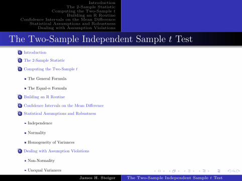
The Two-Sample Independent Sample t Test1 Introduction
2 The 2-Sample Statistic
3 Computing the Two-Sample t
The General Formula
The Equal-n Formula
4 Building an R Routine
5 Confidence Intervals on the Mean Difference
6 Statistical Assumptions and Robustness
Independence
Normality
Homogeneity of Variances
7 Dealing with Assumption Violations
Non-Normality
Unequal Variances
James H. Steiger The Two-Sample Independent Sample t Test

IntroductionThe 2-Sample Statistic
Computing the Two-Sample tBuilding an R Routine
Confidence Intervals on the Mean DifferenceStatistical Assumptions and Robustness
Dealing with Assumption Violations
Introduction
In previous lectures, we dealt with simplest kind of tstatistic, the 1-sample t test for a single mean.This test statistic is actually just the simplest special caseof an entire class of test statistics.In this lecture, we examine perhaps the best known of the tstatistics, the 2-Sample Independent Sample t test forcomparing the means of two groups.Some of the things we learned about the 1-sample t willgeneralize directly to this new situation.
James H. Steiger The Two-Sample Independent Sample t Test

IntroductionThe 2-Sample Statistic
Computing the Two-Sample tBuilding an R Routine
Confidence Intervals on the Mean DifferenceStatistical Assumptions and Robustness
Dealing with Assumption Violations
Introduction
The 2-sample t test is used to assess whether two differentpopulations have the same mean.The most popular use for the test is in the context of the2-group, Experimental-Control group design, in which agroup of subjects is randomly divided into two groups, oneof which receives the experimental treatment, the other acontrol (often some kind of placebo).Let µ1 be the mean of the Experimental group, and µ3 themean of the control group. Then the statistical nullhypothesis is
H0 : µ1 = µ2
Notice that this hypothesis is true, if and only ifµ1 − µ2 = 0, so in a sense it is a hypothesis about the meandifference.
James H. Steiger The Two-Sample Independent Sample t Test
IntroductionThe 2-Sample Statistic
Computing the Two-Sample tBuilding an R Routine
Confidence Intervals on the Mean DifferenceStatistical Assumptions and Robustness
Dealing with Assumption Violations
The 2-Sample Statistic
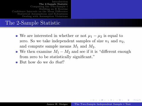
We are interested in whether or not µ1 − µ2 is equal tozero. So we take independent samples of size n1 and n2,and compute sample means M1 and M2.We then examine M1−M2 and see if it is “different enoughfrom zero to be statistically significant.”But how do we do that?
James H. Steiger The Two-Sample Independent Sample t Test

IntroductionThe 2-Sample Statistic
Computing the Two-Sample tBuilding an R Routine
Confidence Intervals on the Mean DifferenceStatistical Assumptions and Robustness
Dealing with Assumption Violations
The 2-Sample StatisticA 2-Sample Z
Although the equations are more complicated, the basicidea is the same.The numerator includes two sample statistics, butultimately reduces them to a single number, M1 −M2.We standardize the mean difference M1 −M2 bysubtracting its null-hypothesized mean, and dividing by itsstandard error.It turns out that the standard error of M1 −M2 is given bythe following formula
σM1−M2 =
√σ21n1
+σ22n2
(1)
Notice that, in the formula, groups can come frompopulations with unequal variances, and the groups canhave unequal sample sizes.The quantity in Equation 1 is called the standard error ofthe difference between means.
James H. Steiger The Two-Sample Independent Sample t Test

IntroductionThe 2-Sample Statistic
Computing the Two-Sample tBuilding an R Routine
Confidence Intervals on the Mean DifferenceStatistical Assumptions and Robustness
Dealing with Assumption Violations
The 2-Sample StatisticA 2-Sample Z
If we knew the two population variances, we couldconstruct a Z-statistic of the form
Z =M1 −M2√σ2
1n1
+σ2
2n2
(2)
This Z-statistic would be the two-sample equivalent of theZ-statistic we saw earlier.But in practice we don’t know the two populationvariances! So what can we do?
James H. Steiger The Two-Sample Independent Sample t Test
IntroductionThe 2-Sample Statistic
Computing the Two-Sample tBuilding an R Routine
Confidence Intervals on the Mean DifferenceStatistical Assumptions and Robustness
Dealing with Assumption Violations
The 2-Sample StatisticSubstituting Sample Variances
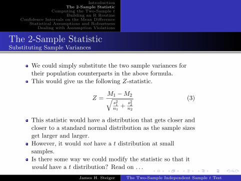
We could simply substitute the two sample variances fortheir population counterparts in the above formula.This would give us the following Z-statistic.
Z =M1 −M2√s21n1
+s22n2
(3)
This statistic would have a distribution that gets closer andcloser to a standard normal distribution as the sample sizesget larger and larger.However, it would not have a t distribution at smallsamples.Is there some way we could modify the statistic so that itwould have a t distribution? Read on . . .
James H. Steiger The Two-Sample Independent Sample t Test

IntroductionThe 2-Sample Statistic
Computing the Two-Sample tBuilding an R Routine
Confidence Intervals on the Mean DifferenceStatistical Assumptions and Robustness
Dealing with Assumption Violations
The 2-Sample StatisticGetting to a t-Statistic
Advanced statistical theory tells us that simplysubstituting sample variances in Equation 2 above will notbe enough to get us to a t-distribution, unless n1 = n2 .However, it turns out that making two simplemodifications in the Z-statistic formula will result in astatistic that does have a t distribution.These two modifications occur in the denominator of theformula.
James H. Steiger The Two-Sample Independent Sample t Test

IntroductionThe 2-Sample Statistic
Computing the Two-Sample tBuilding an R Routine
Confidence Intervals on the Mean DifferenceStatistical Assumptions and Robustness
Dealing with Assumption Violations
The 2-Sample StatisticGetting to a t-Statistic
First, let us incorporate an assumption of equal variances,that is, that both experimental populations have the samevariance.If we are using an experimental-control design, thisamounts to an assumption that the experimental effect actsadditively, that is, scores in the experimental group have,in effect, a constant added to them. (Remember from theearly days of the course that adding a constant to a groupof scores does not change the variance of those scores.)
James H. Steiger The Two-Sample Independent Sample t Test
IntroductionThe 2-Sample Statistic
Computing the Two-Sample tBuilding an R Routine
Confidence Intervals on the Mean DifferenceStatistical Assumptions and Robustness
Dealing with Assumption Violations
The 2-Sample StatisticGetting to a t-Statistic
What would our original Z-statistic look like if we assumedequal variances?One way of approaching this is to simply drop thesubscript on σ21 and σ22, since they are now assumed to bethe same σ2.We’d get
Z =M1 −M2√σ2
n1+ σ2
n2
(4)
But note, there is a common σ2 that can be factored out,resulting in the equation below.
Z =M1 −M2√(1n1
+ 1n2
)σ2
(5)
James H. Steiger The Two-Sample Independent Sample t Test
IntroductionThe 2-Sample Statistic
Computing the Two-Sample tBuilding an R Routine
Confidence Intervals on the Mean DifferenceStatistical Assumptions and Robustness
Dealing with Assumption Violations
The 2-Sample StatisticGetting to a t-Statistic
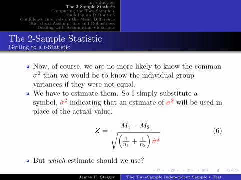
Now, of course, we are no more likely to know the commonσ2 than we would be to know the individual groupvariances if they were not equal.We have to estimate them. So I simply substitute asymbol, σ̂2 indicating that an estimate of σ2 will be used inplace of the actual value.
Z =M1 −M2√(1n1
+ 1n2
)σ̂2
(6)
But which estimate should we use?
James H. Steiger The Two-Sample Independent Sample t Test

IntroductionThe 2-Sample Statistic
Computing the Two-Sample tBuilding an R Routine
Confidence Intervals on the Mean DifferenceStatistical Assumptions and Robustness
Dealing with Assumption Violations
The 2-Sample StatisticGetting to a t-Statistic
There are many possible estimates of σ2 that we couldconstruct from the two sample variances.Remember, we are assuming each of the two samplevariances is estimating the same quantity.It turns out that one particular estimate, if substituted forσ2, yields a statistic that has an exact Student tdistribution.
James H. Steiger The Two-Sample Independent Sample t Test

IntroductionThe 2-Sample Statistic
Computing the Two-Sample tBuilding an R Routine
Confidence Intervals on the Mean DifferenceStatistical Assumptions and Robustness
Dealing with Assumption Violations
The 2-Sample StatisticGetting to a t-Statistic
This estimate goes by a variety of names.It is sometimes called “the pooled unbiased estimator,” andalso sometimes called “Mean Square Within” or “MeanSquare Error.” Gravetter and Walnau call it Mean SquareWithin.I’ll give the specific formula for two groups
σ̂2 =(n1 − 1)s21 + (n2 − 1)s22
n1 + n2 − 2(7)
Note that this can also be written
σ̂2 =SS1 + SS2df1 + df2
(8)
where SS1 stands for the sum of squared deviations insidegroup 1, and SS2 stands for the sum of squared deviationsinside group 2, and dfj is equal to nj − 1 for each group.
James H. Steiger The Two-Sample Independent Sample t Test

IntroductionThe 2-Sample Statistic
Computing the Two-Sample tBuilding an R Routine
Confidence Intervals on the Mean DifferenceStatistical Assumptions and Robustness
Dealing with Assumption Violations
The 2-Sample StatisticGetting to a t-Statistic
Note that σ̂2 is a weighted average of the two samplevariances. Each variances is weighted by its degrees offreedom divided by the total degrees of freedom.This version of the formula is
σ̂2 =
(df1
df1 + df2
)s21 +
(df2
df1 + df2
)s22 (9)
Notice that σ̂2 is a weighted average of the two variances inwhich the weights are positive and add up to 1.Consequently, it must be somewhere between the two s2
values.What would the formula reduce to if the two sample sizesare equal, and consequently both df are the same? (C.P.)
James H. Steiger The Two-Sample Independent Sample t Test

IntroductionThe 2-Sample Statistic
Computing the Two-Sample tBuilding an R Routine
Confidence Intervals on the Mean DifferenceStatistical Assumptions and Robustness
Dealing with Assumption Violations
The 2-Sample StatisticGetting to a t-Statistic
That’s right! If the two df are the same, then
σ̂2 =s21 + s22
2(10)
James H. Steiger The Two-Sample Independent Sample t Test
IntroductionThe 2-Sample Statistic
Computing the Two-Sample tBuilding an R Routine
Confidence Intervals on the Mean DifferenceStatistical Assumptions and Robustness
Dealing with Assumption Violations
The General FormulaThe Equal-n Formula
Computing the 2-Sample tThe General Formula
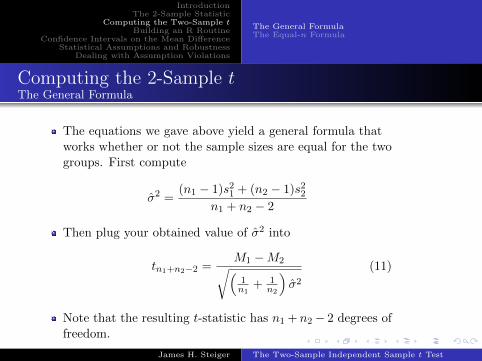
The equations we gave above yield a general formula thatworks whether or not the sample sizes are equal for the twogroups. First compute
σ̂2 =(n1 − 1)s21 + (n2 − 1)s22
n1 + n2 − 2
Then plug your obtained value of σ̂2 into
tn1+n2−2 =M1 −M2√(1n1
+ 1n2
)σ̂2
(11)
Note that the resulting t-statistic has n1 + n2− 2 degrees offreedom.
James H. Steiger The Two-Sample Independent Sample t Test
IntroductionThe 2-Sample Statistic
Computing the Two-Sample tBuilding an R Routine
Confidence Intervals on the Mean DifferenceStatistical Assumptions and Robustness
Dealing with Assumption Violations
The General FormulaThe Equal-n Formula
Computing the 2-Sample tAn Example
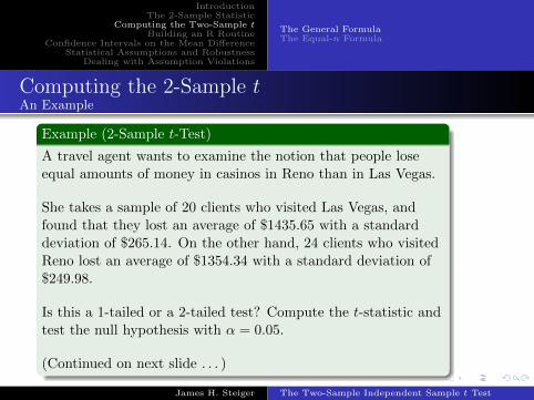
Example (2-Sample t-Test)
A travel agent wants to examine the notion that people loseequal amounts of money in casinos in Reno than in Las Vegas.
She takes a sample of 20 clients who visited Las Vegas, andfound that they lost an average of $1435.65 with a standarddeviation of $265.14. On the other hand, 24 clients who visitedReno lost an average of $1354.34 with a standard deviation of$249.98.
Is this a 1-tailed or a 2-tailed test? Compute the t-statistic andtest the null hypothesis with α = 0.05.
(Continued on next slide . . . )
James H. Steiger The Two-Sample Independent Sample t Test

IntroductionThe 2-Sample Statistic
Computing the Two-Sample tBuilding an R Routine
Confidence Intervals on the Mean DifferenceStatistical Assumptions and Robustness
Dealing with Assumption Violations
The General FormulaThe Equal-n Formula
Computing the 2-Sample tAn Example
Example (2-Sample t-Test)
The null hypothesis is that µ1 = µ2, and the test is 2-tailed. Wefirst compute σ̂2 as
σ̂2 =(n1 − 1)s21 + (n2 − 1)s22
n1 + n2 − 2
=(20− 1)265.142 + (24− 1)249.982
24 + 20− 2
=(19)70299.22 + (23)62490.00
42= 66022.7
(Continued on next slide . . . )
James H. Steiger The Two-Sample Independent Sample t Test
IntroductionThe 2-Sample Statistic
Computing the Two-Sample tBuilding an R Routine
Confidence Intervals on the Mean DifferenceStatistical Assumptions and Robustness
Dealing with Assumption Violations
The General FormulaThe Equal-n Formula
Computing the 2-Sample tAn Example
Example (2-Sample t-Test)
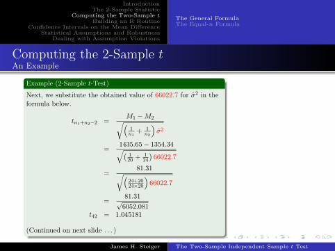
Next, we substitute the obtained value of 66022.7 for σ̂2 in theformula below.
tn1+n2−2 =M1 −M2√(1n1
+ 1n2
)σ̂2
=1435.65− 1354.34√(
120 + 1
24
)66022.7
=81.31√(
24+2024×20
)66022.7
=81.31√
6052.081t42 = 1.045181
(Continued on next slide . . . )
James H. Steiger The Two-Sample Independent Sample t Test

IntroductionThe 2-Sample Statistic
Computing the Two-Sample tBuilding an R Routine
Confidence Intervals on the Mean DifferenceStatistical Assumptions and Robustness
Dealing with Assumption Violations
The General FormulaThe Equal-n Formula
Computing the 2-Sample tAn Example
Example (2-Sample t-Test)
From our knowledge of normal distribution rejection points, andthe fact that those for the t are always larger than the normaldistribution, we know that this obtained value of the t-statisticis not significant.
The Z-statistic would have a critical value of 1.96, and the twill be somewhat higher. How much higher? We can computeit with R as
> qt(0.975,42)
[1] 2.018082
James H. Steiger The Two-Sample Independent Sample t Test
IntroductionThe 2-Sample Statistic
Computing the Two-Sample tBuilding an R Routine
Confidence Intervals on the Mean DifferenceStatistical Assumptions and Robustness
Dealing with Assumption Violations
The General FormulaThe Equal-n Formula
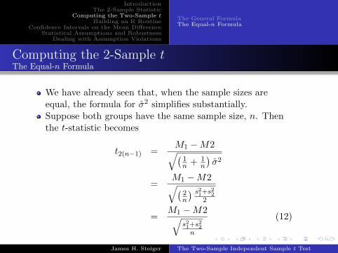
Computing the 2-Sample tThe Equal-n Formula
We have already seen that, when the sample sizes areequal, the formula for σ̂2 simplifies substantially.Suppose both groups have the same sample size, n. Thenthe t-statistic becomes
t2(n−1) =M1 −M2√(
1n + 1
n
)σ̂2
=M1 −M2√(
2n
) s21+s222
=M1 −M2√
s21+s22
n
(12)
James H. Steiger The Two-Sample Independent Sample t Test

IntroductionThe 2-Sample Statistic
Computing the Two-Sample tBuilding an R Routine
Confidence Intervals on the Mean DifferenceStatistical Assumptions and Robustness
Dealing with Assumption Violations
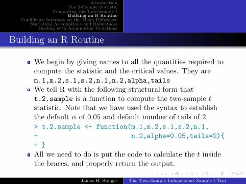
Building an R Routine
Computing the t-statistic with two unequal sized samples ishard work.This is what computers are for.So let’s construct an R function to compute the 2-sample t,and then we may never have to compute it “by hand”again!
James H. Steiger The Two-Sample Independent Sample t Test
IntroductionThe 2-Sample Statistic
Computing the Two-Sample tBuilding an R Routine
Confidence Intervals on the Mean DifferenceStatistical Assumptions and Robustness
Dealing with Assumption Violations
Building an R Routine
We begin by giving names to all the quantities required tocompute the statistic and the critical values. They arem.1,m.2,s.1,s.2,n.1,n.2,alpha,tails
We tell R with the following structural form thatt.2.sample is a function to compute the two-sample tstatistic. Note that we have used the syntax to establishthe default α of 0.05 and default number of tails of 2.
> t.2.sample <- function(m.1,m.2,s.1,s.2,n.1,
+ n.2,alpha=0.05,tails=2){
+ }
All we need to do is put the code to calculate the t insidethe braces, and properly return the output.
James H. Steiger The Two-Sample Independent Sample t Test

IntroductionThe 2-Sample Statistic
Computing the Two-Sample tBuilding an R Routine
Confidence Intervals on the Mean DifferenceStatistical Assumptions and Robustness
Dealing with Assumption Violations
Building an R Routine
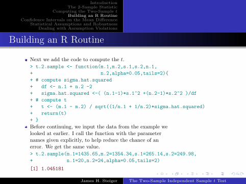
First we add the code to compute σ̂2.
> t.2.sample <- function(m.1,m.2,s.1,s.2,n.1,
+ n.2,alpha=0.05,tails=2){
+ # compute sigma.hat.squared
+ df <- n.1 + n.2 -2
+ sigma.hat.squared <-( (n.1-1)*s.1^2 +(n.2-1)*s.2^2 )/df
+
+ }
James H. Steiger The Two-Sample Independent Sample t Test
IntroductionThe 2-Sample Statistic
Computing the Two-Sample tBuilding an R Routine
Confidence Intervals on the Mean DifferenceStatistical Assumptions and Robustness
Dealing with Assumption Violations
Building an R Routine
Next we add the code to compute the t.
> t.2.sample <- function(m.1,m.2,s.1,s.2,n.1,
+ n.2,alpha=0.05,tails=2){
+ # compute sigma.hat.squared
+ df <- n.1 + n.2 -2
+ sigma.hat.squared <-( (n.1-1)*s.1^2 +(n.2-1)*s.2^2 )/df
+ # compute t
+ t <- (m.1 - m.2) / sqrt((1/n.1 + 1/n.2)*sigma.hat.squared)
+ return(t)
+ }
Before continuing, we input the data from the example welooked at earlier. I call the function with the parameternames given explicitly, to help reduce the chance of anerror. We get the same value.
> t.2.sample(m.1=1435.65,m.2=1354.34,s.1=265.14,s.2=249.98,
+ n.1=20,n.2=24,alpha=0.05,tails=2)
[1] 1.045181
James H. Steiger The Two-Sample Independent Sample t Test

IntroductionThe 2-Sample Statistic
Computing the Two-Sample tBuilding an R Routine
Confidence Intervals on the Mean DifferenceStatistical Assumptions and Robustness
Dealing with Assumption Violations
Building an R Routine
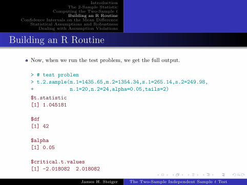
Next we add the code to compute the critical value fromthe t.
> t.2.sample <- function(m.1,m.2,s.1,s.2,n.1,
+ n.2,alpha=0.05,tails=2){
+ # compute sigma.hat.squared
+ df <- n.1 + n.2 -2
+ sigma.hat.squared <-( (n.1-1)*s.1^2 +(n.2-1)*s.2^2 )/df
+ # compute t
+ t <- (m.1 - m.2) / sqrt((1/n.1 + 1/n.2)*sigma.hat.squared)
+ # compute critical value
+ if(tails == -1) p <- alpha
+ if(tails == 1) p <- 1-alpha
+ if(tails == 2) p <- c(alpha/2,1 - alpha/2)
+ crit <- qt(p,df)
+ # create a list of named quantities and return it
+ res <- list(t.statistic = t, df = df, alpha = alpha,
+ critical.t.values = crit)
+ return(res)
+ }
James H. Steiger The Two-Sample Independent Sample t Test
IntroductionThe 2-Sample Statistic
Computing the Two-Sample tBuilding an R Routine
Confidence Intervals on the Mean DifferenceStatistical Assumptions and Robustness
Dealing with Assumption Violations
Building an R Routine
Now, when we run the test problem, we get the full output.
> # test problem
> t.2.sample(m.1=1435.65,m.2=1354.34,s.1=265.14,s.2=249.98,
+ n.1=20,n.2=24,alpha=0.05,tails=2)
$t.statistic
[1] 1.045181
$df
[1] 42
$alpha
[1] 0.05
$critical.t.values
[1] -2.018082 2.018082
James H. Steiger The Two-Sample Independent Sample t Test
IntroductionThe 2-Sample Statistic
Computing the Two-Sample tBuilding an R Routine
Confidence Intervals on the Mean DifferenceStatistical Assumptions and Robustness
Dealing with Assumption Violations
Confidence Intervals on the Mean Difference
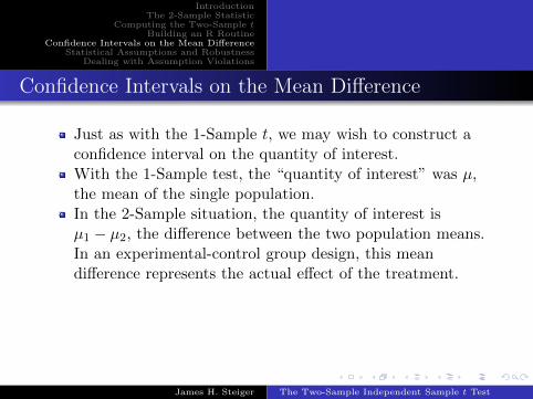
Just as with the 1-Sample t, we may wish to construct aconfidence interval on the quantity of interest.With the 1-Sample test, the “quantity of interest” was µ,the mean of the single population.In the 2-Sample situation, the quantity of interest isµ1 − µ2, the difference between the two population means.In an experimental-control group design, this meandifference represents the actual effect of the treatment.
James H. Steiger The Two-Sample Independent Sample t Test

IntroductionThe 2-Sample Statistic
Computing the Two-Sample tBuilding an R Routine
Confidence Intervals on the Mean DifferenceStatistical Assumptions and Robustness
Dealing with Assumption Violations
Confidence Intervals on the Mean Difference
The formula for the 1− α confidence interval is
M1 −M2 ± t1−α/2,n1+n2−2√
(1/n1 + 1/n2)σ̂2 (13)
Note that the left part of the formula is simply thenumerator of the t statistic, and the right side of theformula is a critical value of t multiplied by thedenominator of the t-statistic.
James H. Steiger The Two-Sample Independent Sample t Test

IntroductionThe 2-Sample Statistic
Computing the Two-Sample tBuilding an R Routine
Confidence Intervals on the Mean DifferenceStatistical Assumptions and Robustness
Dealing with Assumption Violations
IndependenceNormalityHomogeneity of Variances
Introduction
The statistical assumptions of the classic two-sampleindependent sample t are
1 Independence of observations. Each observation isindependent. The classic formula for the sampling varianceof the sample mean, σ2/n, is based on this assumption.
2 Normality. The distribution of the populations is assumedto be normal.
3 Homogeneity of variances. The populations are assumed tohave equal variances.
We need to consider, in turn,1 How violations of these assumptions affect performance of
the t-test.2 What methods are available to produce reasonable
inferential performance when assumptions are violated.3 How to detect violations of assumptions.
James H. Steiger The Two-Sample Independent Sample t Test
IntroductionThe 2-Sample Statistic
Computing the Two-Sample tBuilding an R Routine
Confidence Intervals on the Mean DifferenceStatistical Assumptions and Robustness
Dealing with Assumption Violations
IndependenceNormalityHomogeneity of Variances
Effect of ViolationsIndependence
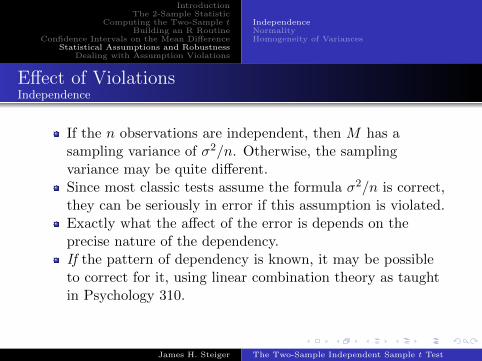
If the n observations are independent, then M has asampling variance of σ2/n. Otherwise, the samplingvariance may be quite different.Since most classic tests assume the formula σ2/n is correct,they can be seriously in error if this assumption is violated.Exactly what the affect of the error is depends on theprecise nature of the dependency.If the pattern of dependency is known, it may be possibleto correct for it, using linear combination theory as taughtin Psychology 310.
James H. Steiger The Two-Sample Independent Sample t Test

IntroductionThe 2-Sample Statistic
Computing the Two-Sample tBuilding an R Routine
Confidence Intervals on the Mean DifferenceStatistical Assumptions and Robustness
Dealing with Assumption Violations
IndependenceNormalityHomogeneity of Variances
Effect of ViolationsNormality
A key fact about the normal distribution is that the samplemean and sample variance of a set of observations takenrandomly from a normal population are independent.This independence of the mean and variance are crucial inthe derivation of Student’s t distribution.When populations are not normal, this lack ofindependence can lead to poor performance of the t-test.
James H. Steiger The Two-Sample Independent Sample t Test

IntroductionThe 2-Sample Statistic
Computing the Two-Sample tBuilding an R Routine
Confidence Intervals on the Mean DifferenceStatistical Assumptions and Robustness
Dealing with Assumption Violations
IndependenceNormalityHomogeneity of Variances
Effect of ViolationsNormality
Violations of normality can occur in several distinct ways.The general shape of the distribution can be skewed, insome cases for obvious reasons related to the nature of themeasurement process.There can be contamination by outliers. These extreme andunusual observations lead to the distribution having tailsthat are much longer than seen with a normal distribution.Yet, if the contamination probability is small, it may bedifficult to diagnose outlier problems when they occur. Forexample, are the outliers the result of:
1 A mixture of two or more processes (or subgroups) thatcharacterize the population of interest?
2 A random measurement error?
James H. Steiger The Two-Sample Independent Sample t Test

IntroductionThe 2-Sample Statistic
Computing the Two-Sample tBuilding an R Routine
Confidence Intervals on the Mean DifferenceStatistical Assumptions and Robustness
Dealing with Assumption Violations
IndependenceNormalityHomogeneity of Variances
Effect of ViolationsNormality
High skewness or kurtosis can lead to Type I error ratesthat are either much higher or much lower than thenominal rates.Contamination by outliers can lead to a significant loss ofpower when the null hypothesis is false.
James H. Steiger The Two-Sample Independent Sample t Test

IntroductionThe 2-Sample Statistic
Computing the Two-Sample tBuilding an R Routine
Confidence Intervals on the Mean DifferenceStatistical Assumptions and Robustness
Dealing with Assumption Violations
IndependenceNormalityHomogeneity of Variances
Effect of ViolationsHomogeneity of Variances
As we saw earlier, the denominator of the 2-Samplet-statistic explicitly assumes equal variances.Recall that, with independent samples, the variance ofM1 −M2 is
Var(M1 −M2) =σ21n1
+σ22n2
(14)
The t statistic replaces this formula with one that assumesequal variances, i.e.,
Var(M1 −M2) =
(1
n1+
1
n2
)σ2 (15)
and then substitutes the estimate σ̂2 for σ2, where
σ̂2 =(n1 − 1)s21 + (n2 − 1)s22
n1 + n2 − 2(16)
James H. Steiger The Two-Sample Independent Sample t Test

IntroductionThe 2-Sample Statistic
Computing the Two-Sample tBuilding an R Routine
Confidence Intervals on the Mean DifferenceStatistical Assumptions and Robustness
Dealing with Assumption Violations
IndependenceNormalityHomogeneity of Variances
Effect of ViolationsHomogeneity of Variances
Notice that, in the preceding formula, we are essentiallysubstituting the (weighted) average of the two variances foreach variance in the formula for the sampling variance ofM1 −M2.If the assumption of equal variances is correct, theresulting formula will be a consistent estimate of thecorrect quantity.What will the effect be if the assumption of equal variancesis incorrect?How can we approximate the impact of a violation of theequal variances assumption on the true Type I error rate ofthe t-test when the null hypothesis is true?
James H. Steiger The Two-Sample Independent Sample t Test

IntroductionThe 2-Sample Statistic
Computing the Two-Sample tBuilding an R Routine
Confidence Intervals on the Mean DifferenceStatistical Assumptions and Robustness
Dealing with Assumption Violations
IndependenceNormalityHomogeneity of Variances
Effect of ViolationsHomogeneity of Variances
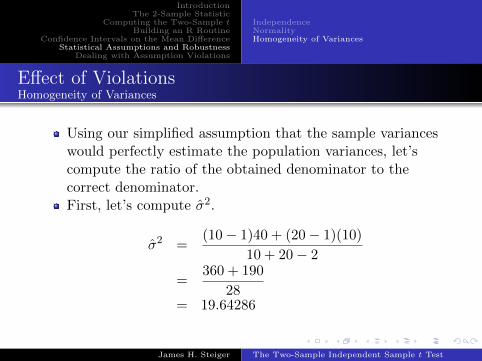
One simplified approach would be two assume that there isno sampling error in the sample variances, i.e., that s21 = σ21and s22 = σ22, and measure the result of the violation ofassumptions.For example, suppose σ21 = 40, and σ22 = 10, while n1 = 10and n2 = 20. What will the approximate effect on the trueα?
James H. Steiger The Two-Sample Independent Sample t Test
IntroductionThe 2-Sample Statistic
Computing the Two-Sample tBuilding an R Routine
Confidence Intervals on the Mean DifferenceStatistical Assumptions and Robustness
Dealing with Assumption Violations
IndependenceNormalityHomogeneity of Variances
Effect of ViolationsHomogeneity of Variances
Using our simplified assumption that the sample varianceswould perfectly estimate the population variances, let’scompute the ratio of the obtained denominator to thecorrect denominator.First, let’s compute σ̂2.
σ̂2 =(10− 1)40 + (20− 1)(10)
10 + 20− 2
=360 + 190
28= 19.64286
James H. Steiger The Two-Sample Independent Sample t Test

IntroductionThe 2-Sample Statistic
Computing the Two-Sample tBuilding an R Routine
Confidence Intervals on the Mean DifferenceStatistical Assumptions and Robustness
Dealing with Assumption Violations
IndependenceNormalityHomogeneity of Variances
Effect of ViolationsHomogeneity of Variances
The obtained denominator is then√V̂ar(M1 −M2) =
√(1
n1+
1
n2
)σ̂2
=
√(1
10+
1
20
)19.64286
=√
2.946429
= 1.716516
James H. Steiger The Two-Sample Independent Sample t Test
IntroductionThe 2-Sample Statistic
Computing the Two-Sample tBuilding an R Routine
Confidence Intervals on the Mean DifferenceStatistical Assumptions and Robustness
Dealing with Assumption Violations
IndependenceNormalityHomogeneity of Variances
Effect of ViolationsHomogeneity of Variances
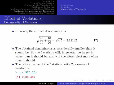
However, the correct denominator is√40
10+
10
20=√
4.5 = 2.12132 (17)
The obtained denominator is considerably smaller than itshould be. So the t statistic will, in general, be larger invalue than it should be, and will therefore reject more oftenthan it should.The critical value of the t statistic with 28 degrees offreedom is
> qt(.975,28)
[1] 2.048407
James H. Steiger The Two-Sample Independent Sample t Test
IntroductionThe 2-Sample Statistic
Computing the Two-Sample tBuilding an R Routine
Confidence Intervals on the Mean DifferenceStatistical Assumptions and Robustness
Dealing with Assumption Violations
IndependenceNormalityHomogeneity of Variances
Effect of ViolationsHomogeneity of Variances
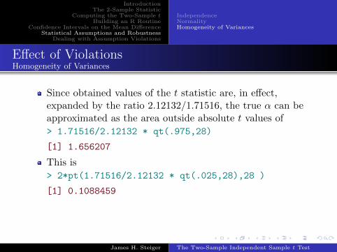
Since obtained values of the t statistic are, in effect,expanded by the ratio 2.12132/1.71516, the true α can beapproximated as the area outside absolute t values of
> 1.71516/2.12132 * qt(.975,28)
[1] 1.656207
This is
> 2*pt(1.71516/2.12132 * qt(.025,28),28 )
[1] 0.1088459
James H. Steiger The Two-Sample Independent Sample t Test

IntroductionThe 2-Sample Statistic
Computing the Two-Sample tBuilding an R Routine
Confidence Intervals on the Mean DifferenceStatistical Assumptions and Robustness
Dealing with Assumption Violations
IndependenceNormalityHomogeneity of Variances
Effect of ViolationsHomogeneity of Variances
The above estimate of .109 was obtained with a simplifyingassumption, and is an approximation.An alternative approach is Monte Carlo simulation. I ran at-test 10,000 times under the above conditions and theType I error rate was .1155.This confirms that the true α is more than twice as large asthe nominal α of .05.
James H. Steiger The Two-Sample Independent Sample t Test
IntroductionThe 2-Sample Statistic
Computing the Two-Sample tBuilding an R Routine
Confidence Intervals on the Mean DifferenceStatistical Assumptions and Robustness
Dealing with Assumption Violations
IndependenceNormalityHomogeneity of Variances
Effect of ViolationsHomogeneity of Variances
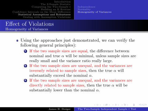
Using the approaches just demonstrated, we can verify thefollowing general principles):
1 If the two sample sizes are equal, the difference betweennominal and true α will be minimal, unless sample sizes arereally small and the variance ratio really large.
2 If the two sample sizes are unequal, and the variances areinversely related to sample sizes, then the true α willsubstantially exceed the nominal α.
3 If the two sample sizes are unequal, and the variances aredirectly related to sample sizes, then the true α will besubstantially lower than the nominal α.
James H. Steiger The Two-Sample Independent Sample t Test

IntroductionThe 2-Sample Statistic
Computing the Two-Sample tBuilding an R Routine
Confidence Intervals on the Mean DifferenceStatistical Assumptions and Robustness
Dealing with Assumption Violations
Non-NormalityUnequal Variances
Dealing with Non-Normality
When data show a recognized non-normal distribution, onehas recourse to several options:
1 Do nothing. If violation of normality is not severe, the t-testmay be reasonably robust.
2 Transform the data. This seems especially justifiable if thedata have a similar non-normal shape. With certain kindsof shapes, certain transformations will convert thedistributions to be closer to normality. However, thisapproach is generally not recommended, for a variety ofreasons.
3 Trim the data. By trimming a percentage of the moreextreme cases from the data, the skewness and kurtosis maybe brought more into line with those of a normaldistribution.
4 Use a non-parametric procedure. Tests for equality of meansthat do not assume normality are available. However, theygenerally assume that the two samples have equaldistributions, not that they simply have equal means (ormedians).
James H. Steiger The Two-Sample Independent Sample t Test
IntroductionThe 2-Sample Statistic
Computing the Two-Sample tBuilding an R Routine
Confidence Intervals on the Mean DifferenceStatistical Assumptions and Robustness
Dealing with Assumption Violations
Non-NormalityUnequal Variances
Dealing with Non-Normality
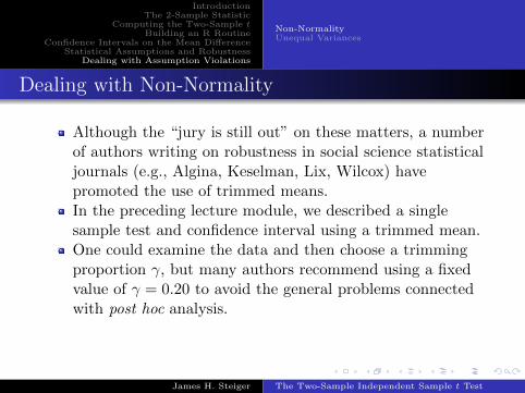
Although the “jury is still out” on these matters, a numberof authors writing on robustness in social science statisticaljournals (e.g., Algina, Keselman, Lix, Wilcox) havepromoted the use of trimmed means.In the preceding lecture module, we described a singlesample test and confidence interval using a trimmed mean.One could examine the data and then choose a trimmingproportion γ, but many authors recommend using a fixedvalue of γ = 0.20 to avoid the general problems connectedwith post hoc analysis.
James H. Steiger The Two-Sample Independent Sample t Test

IntroductionThe 2-Sample Statistic
Computing the Two-Sample tBuilding an R Routine
Confidence Intervals on the Mean DifferenceStatistical Assumptions and Robustness
Dealing with Assumption Violations
Non-NormalityUnequal Variances
Dealing with Unequal VariancesThe Welch Test
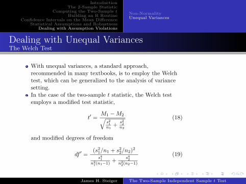
With unequal variances, a standard approach,recommended in many textbooks, is to employ the Welchtest, which can be generalized to the analysis of variancesetting.In the case of the two-sample t statistic, the Welch testemploys a modified test statistic,
t′ =M1 −M2√s21n1
+s22n2
(18)
and modified degrees of freedom
df ′ =(s21/n1 + s22/n2)
2
s41n2
1(n1−1)+
s42n2
2(n2−1)
(19)
James H. Steiger The Two-Sample Independent Sample t Test
IntroductionThe 2-Sample Statistic
Computing the Two-Sample tBuilding an R Routine
Confidence Intervals on the Mean DifferenceStatistical Assumptions and Robustness
Dealing with Assumption Violations
Non-NormalityUnequal Variances
Dealing with Unequal VariancesThe Welch Test
With unequal variances, a standard approach,recommended in many textbooks, is to employ the Welchtest, which can be generalized to the analysis of variancesetting.In the case of the two-sample t statistic, the Welch testemploys a modified test statistic,
t′ =M1 −M2√s21n1
+s22n2
(18)
and modified degrees of freedom
df ′ =(s21/n1 + s22/n2)
2
s41n2
1(n1−1)+
s42n2
2(n2−1)
(19)
James H. Steiger The Two-Sample Independent Sample t Test
IntroductionThe 2-Sample Statistic
Computing the Two-Sample tBuilding an R Routine
Confidence Intervals on the Mean DifferenceStatistical Assumptions and Robustness
Dealing with Assumption Violations
Non-NormalityUnequal Variances
General Testing StrategyThe Welch Test
How should one employ the Welch test?Some authors advocate a sequential strategy, in which onefirst tests for equal variances. If the equal variance testrejects, employ the Welch test, otherwise employ thestandard t-test.This is, at its foundation, an “Accept-Support” strategy, inwhich one employs the standard test if the null hypothesisis not rejected.The fact that tests on variances have low powercompromises this strategy.As a result, some authors advocate always doing a Welchtest.
James H. Steiger The Two-Sample Independent Sample t Test