the unequal geographic burden of federal taxationdavidalbouy.net/federaltaxes.pdf · federal tax...

635

[ Journal of Political Economy, 2009, vol. 117, no. 4]� 2009 by The University of Chicago. All rights reserved. 0022-3808/2009/11704-0002$10.00

The Unequal Geographic Burden of FederalTaxation

David AlbouyUniversity of Michigan and National Bureau of Economic Research

In the United States, workers in cities offering above-average wages—cities with high productivity, low quality of life, or inefficient housingsectors—pay 27 percent more in federal taxes than otherwise identicalworkers in cities offering below-average wages. According to simula-tion results, taxes lower long-run employment levels in high-wage areasby 13 percent and land and housing prices by 21 and 5 percent,causing locational inefficiencies costing 0.23 percent of income, or$28 billion in 2008. Employment is shifted from north to south andfrom urban to rural areas. Tax deductions index taxes partially to localcost of living, improving locational efficiency.

I. Introduction

Wage and cost-of-living levels vary considerably across cities in theUnited States, yet the federal tax code does not take this variation into

I thank Alan Auerbach, Timothy Bartik, David Card, Allan Collard-Wexler, Tom Davidoff,Gilles Duranton, Rob Gillezeau, Erica Greulich, Jim Hines, Darren Lubotsky, Bert Lue,Erin Metcalf, Enrico Moretti, John Quigley, Marit Rehavi, Emmanuel Saez, and WilliamStrange; participants of seminars at Chicago-Harris, Michigan, Northwestern, New YorkUniversity, the Philadelphia Federal Reserve Bank, Public Policy Institute of California,Syracuse, Toronto-Rotman, University of California, Berkeley, University of California, SanDiego, University of Texas at Austin, and Wisconsin; and presentations at the 2007 NBERSummer Institute on Taxation, 2007 National Tax Association Annual Meetings, and 2009Centre for Economic Policy and Research Public Policy Symposium for their help, input,and advice. Furthermore, I am grateful to the Burch Center for Tax Policy and PublicFinance and the Fisher Center for Real Estate and Urban Economics for their financialassistance, as well as the National Tax Association, the W. E. Upjohn Institute for Em-ployment Research, and the American Real Estate and Urban Economics Association forgenerously awarding my dissertation, “Causes and Consequences of Unequal Federal Tax-ation and Spending across Regions,” which this article is based on. Any mistakes are myown.

636 journal of political economy

account. Since federal taxes are based on nominal incomes, workerswith the same real income pay higher taxes in high-cost areas than inlow-cost areas, without receiving additional benefits. Recognizing this,the Tax Foundation (Dubay 2006, 1) argues, “the nation is not onlyredistributing income from the prosperous to the poor, but from themiddle-income residents of high-cost states to the middle-income resi-dents of low-cost states.” While the Tax Foundation has suggested a flattax to remedy this problem (Hoffman and Moody 2003), politiciansfrom high-cost areas have proposed indexing federal taxes and benefitsto local costs, arguing that workers with the same real incomes shouldpay the same nominal taxes.

For federal taxes to not distort the location choices of workers, thecorrect principle is that taxes should be independent of where workerslive so that location-wise they are effectively lump sum. The currentsystem taxes workers more for taking jobs in higher-paying cities, blunt-ing the incentive to live in these cities, characterized by high firm pro-ductivity and low quality of life. For example, in the New York metro-politan area, wage levels are 21 percent above the national average,which, interacted with an effective marginal tax rate of 33 percent,creates a 7 percent federal surtax on labor income for locating there.Unlike local tax differences, federal tax differences of this kind are notcompensated with higher levels of local spending and may thereforeaffect location choices substantially.

Because federal taxes are not indexed to local wage levels, workersare induced to leave cities with high wages and move to cities with lowwages. As a result, unindexed federal taxes lower employment levels andproperty values in high-wage cities while having the opposite effect onlow-wage cities. In equilibrium, these price changes compensate workersfor federal tax differences across cities, but the resulting geographicdistribution of employment is inefficient, reducing overall welfare.

The unequal distribution of federal taxes that results from wage dif-ferences across cities does not depend on the progressivity of taxes andcannot be eliminated with a flat tax. The view that workers with thesame real incomes should pay the same nominal taxes holds true acrosscities that vary in the productivity of their firms, as nominal incomesmerely track cost-of-living differences across these cities. However, thisview is incorrect across cities that vary in quality of life, as nicer citieshave a higher cost of living but lower nominal wage levels and hencea lower federal tax burden. Indexing the tax code to local costs wouldeliminate federal tax differences across cities that vary in productivitybut exacerbate them across cities that vary in quality of life.

An empirical simulation for the United States, below, reveals thatworkers with the same skills pay up to 27 percent more in federal taxesin high-wage cities than in low-wage cities. The federal government

federal tax burden 637

effectively taxes workers for living in large cities while subsidizing themto live in rural areas. Taxes also fall more heavily on the Northeast,Pacific, and Great Lakes regions and less on the South. Controlling forsocioeconomic disparities, approximately $270 billion each year aretransferred horizontally from high-wage areas to low-wage areas. Thesefindings partly confirm Senator Patrick Moynihan’s (2000) claims in 24years of reports, entitled The Federal Budget and the States, that the “federalbalance of payments” across areas is highly unequal, although thesereports do not control for socioeconomic differences across regions,nor do they consider the effects on local employment or prices.

Journalist Malcolm Gladwell (1996) writes that the inequality in thefederal balance of payments “is according to urban experts and econ-omists one of the best-kept secrets in American politics” and that “thedecline of many northeastern American cities may be due not just tomismanagement—as is now popularly imagined—but to the emptyingof their coffers by the federal government.” Such a view is supportedby the simulation: over the long run, federal taxes have lowered em-ployment, housing prices, and land values in high-wage areas by 13, 5,and 21 percent, respectively, and done the opposite in low-wage areas.Overall, federal taxes have tilted the geographic distribution of em-ployment away from the North toward the South and away from urbanareas toward rural areas, creating a welfare loss estimated at 0.23 percentof income, or $28 billion in 2008. Without federal tax deductions formortgage interest and local taxes, this loss would be even larger.

Previous research about how federal taxes interact with local pricescontains some important findings but has been too narrow or informalto guide policy comprehensively. Wildasin (1980) finds that federal taxeson labor income cause mobile workers to locate inefficiently across citiesoffering different wages but focuses on conditions characterizing effi-ciency rather than the results of inefficiency. Without referring specif-ically to taxation, Glaeser (1998) argues that federal transfer levelsshould not be tied to local price levels, as this implicitly subsidizes re-cipients to live in expensive, high-quality-of-life cities. More generally,Kaplow (1995) and Knoll and Griffith (2003) also allow productivitydifferences to affect local wages and prices, leading them to considerthe benefits of indexing taxes to local wages. Although insightful, theirinformal arguments leave open the exact consequences of failing toindex the tax code, raising the need for more rigorous quantitativeanalysis.1

1 Kaplow’s (1995) analysis holds prices fixed and presents an index formula that doesnot equalize nominal tax payments across areas. Knoll and Griffith (2003) assume that aflat tax on income does not change prices or reallocate resources; this assumption, asshown below, does not hold in general equilibrium. Other work considers how tax de-ductions interact with local prices. Research by Gyourko and Sinai (2003, 2004) and Brady,


Section II introduces a model of mobile workers who live in citieswith attributes that generate differences in costs of living, wages, andfederal tax burdens. Section III describes the federal tax differencesthat arise in equilibrium and how they affect local prices. Section IVexamines how taxes distort location decisions and how to calculate theresulting efficiency loss. Then, Section V considers the effect of indexingtaxes to local wages or costs of living and demonstrates how tax de-ductions for locally produced goods, such as housing, produce a mildform of cost indexation. Section VI calibrates the model and simulateshow differential taxes affect the distribution of local prices, employment,and welfare, taking into account differential federal spending patterns.

II. Theoretical Setup

To explain why prices and tax burdens differ across cities, I adapt thegeneral-equilibrium model of Rosen (1979) and Roback (1980, 1982),incorporating federal taxes. The national economy is closed and con-tains many cities, indexed by j, which trade with each other and sharea homogeneous population of mobile workers. These workers consumea numeraire traded good, x, and a nontraded “home” good, y, with localprice . Cities differ in three types of exogenous attributes. Quality ofjplife, , may be affected by amenities such as weather or safety. Pro-jQductivity in the traded-good sector, (or “trade productivity”), may bejA X

due to natural advantages, such as a harbor, or to agglomeration econ-omies, such as input sharing. Productivity in the home-good sector,

(or “home productivity”), may be affected by natural advantages orjA Y

regulations affecting residential housing. The average value of eachattribute is set to one. Although some city attributes may indeed beendogenous, it is safe to consider them exogenous if federal taxes donot significantly affect their relative levels across cities.

Firms produce traded and home goods out of land, capital, and labor.Factors receive the same payment in either sector. Land, , is fixed inLsupply in each city at and is paid a city-specific price, . Capital, ,j jL r Kis fully mobile and is paid the price everywhere. The supply of capitaliin each city is denoted , with the aggregate level of capital fixed atjK

; thus . Labor, , is also fully mobile, but becauseTOT j TOTK � K p K Nj

workers care about local prices and quality of life, wages, , may varyjwacross cities. Workers have identical tastes and endowments, and each

Cronin, and Houser (2003) tabulates how mortgage and local-tax deductions dispropor-tionately benefit high-cost areas but neglects how these deductions may offset the unequalburden of federal taxes from wage differences. Surveys of the possible benefits of taxdeductions for mortgage interest (e.g., Glaeser and Shapiro 2003) or local taxes (e.g.,Kaplow 1996) do not consider their interurban locational effects.


supplies a single unit of labor. The total number of workers is fixed at, so . Workers own identical diversified portfolios ofTOT j TOTN � N p Nj

land and capital, which pay an income from landTOT j jR p (1/N ) � r Lj

and from capital. Total income var-TOT TOT j j¯I p i (K /N ) m { R � I � wies across cities only as wages vary. Out of this income, workers pay afederal income tax of . Deductions are introduced in Section V.2jt(m )

Workers’ preferences are modeled by a utility function, ,U(x, y; Q)that is quasi-concave and homothetic over and and increasing inx y

. The corresponding expenditure function isQ e[p, u, t(m); Q] {; is assumed to enter neutrallymin [x � py � t(m) : U(x, y; Q) ≥ u] Qx,y

into the utility function and is normalized so that e[p, u, t(m); Q] p, where . Since workers are fully[e(p, u) � t(m)]/Q e(p, u) { e(p, u, 0; 1)

mobile, their utility must be the same across all inhabited cities so thathigher prices, lower quality of life, or higher taxes must be compensatedwith greater income:

j j j j¯[e(p , u) � t(m )]/Q p m ; (1)

is the level of utility attained by all workers, regardless of each worker’sufederal tax burden.3

Operating under perfect competition, firms produce traded andhome goods according to the functions andX p A F (L , N , K )X X X X X

, where and are concave and exhibit constantY p A F (L , N , K ) F FY Y Y Y Y X Y

returns to scale.4 Unit cost in the traded-good sector is c (r, w, i)/A {X X

. A symmetric definition holdsmin [rL � wN � iK : A F(L, N, K) p 1]L,N,K X

for unit cost in the home-good sector, . All factors are fully employed:cY

, , and . As markets are com-j j j j j j j j jL � L p L N � N p N K � K p KX Y X Y X Y

petitive, firms make zero profits in equilibrium so that for given outputprices, more productive cities pay higher rents and wages, and the fol-lowing conditions hold in all cities where production occurs:j

j j j¯c (r , w , i )/A p 1, (2)X X

j j j j¯c (r , w , i )/A p p . (3)Y Y

2 Because markets are perfectly competitive, the economic incidence is unchanged ifthe nominal incidence of taxes is placed on firms’ labor costs rather than on workers’wage incomes. Consumption taxes in this model are equivalent to income taxes; taxes onproduction are largely equivalent, except for the portion that falls on capital and land.

3 The model generalizes to a case with workers that supplies different fixed amounts oflabor if these workers are perfect substitutes in production, have identical homotheticpreferences, and earn equal shares of income from labor. More general types of workerheterogeneity are considered in Albouy (2008b), including the case in which some workersare immobile or differ in their attachment to particular cities, simulating the effects ofmoving costs. This explains how federal tax changes can have redistributive effects acrossareas when tastes are heterogeneous or moving costs are substantial.

4 Non-Hicks-neutral productivity differences have similar impacts on relative prices acrosscities but not on relative quantities.


This analysis models a single federal government that collects taxrevenues, makes transfers, and uses the net balance to buy traded goodsthat are transformed into a federal public good, such as defense. Thisfederal public good benefits workers everywhere equally, and its levelis held fixed. Federal taxes are modeled net of federal transfers. Nat-urally, federal means-tested benefits increase the effective marginal taxrate for some workers.5 In addition, it matters if federal tax paymentsare tied to federal transfers. In the United States, workers in high-wageareas pay more in payroll taxes and then receive higher social securitybenefits later in life. Thus, the marginal benefit of paying these taxesshould be subtracted from the effective marginal income tax rate.

The local public sector does not need to be modeled explicitly. Iflocal government provides goods efficiently, as in the Tiebout (1956)model, these goods can be treated as consumption goods. Furthermore,efficiency differences across local public sectors may be subsumed intodifferences in (Gyourko and Tracy 1989, 1991) or . Taxes leviedj jQ A Y

at the subnational level can also be distributed unequally across areaswhen wages vary within a subnational jurisdiction, such as a state. Statetaxes are incorporated into the simulation below, in which their effectsare small; for expositional ease, they are ignored here.

For workers, denote the expenditure shares of traded goods, homegoods, and taxes as , and ; denotej j j j j j j j j js { x /m , s { p y /m s p t(m )/mx y T

the shares of income received from land, labor, and capital income as, , and . For firms, denote the cost sharesj j j j j j js { R/m s { w /m s { I/mR w I

of land, labor, and capital in the traded-good sector as ,j j j jv { r L /XL X

, and ; denote similar cost shares in thej j j j j j j¯v { w N /X v { i K /XN X K X

home-good sector as , and . Assume, as is likely, that homej j jf , f fL N K

goods are more cost intensive in land relative to labor than traded goods,that is, .j j j jf /f 1 v /vL N L N

III. Price and Federal Tax Differences across Cities

Federal taxes on labor income affect how prices vary cross-sectionallyacross cities with different attributes. To analyze this, assume that thereare enough cities varying in the three city attributes, , and , toQ , A AX Y

treat these attributes as continuous variables. The equilibrium condi-

5 This is complicated by eligibility requirements for programs that vary by state or county.Furthermore, some benefit levels are tied to local prices, such as housing programs,although these programs tend to be small. Inasmuch as they are valued, local goodsprovided by the federal government may be treated as transfers, as can intergovernmentaltransfers that increase the supply of local government goods. It should be noted thatfederal matching rates for many programs (e.g., Medicaid) decline with average stateincome. The complicated nature of these transfers makes it useful to consider some federaltransfers separately from an overall tax schedule, as in Sec. VI.D.


tions (1), (2), and (3) implicitly define the prices , , and —andj j jw r pthe federal tax, which depends on them—as a function ofj jt(m ), Q ,

, and . These conditions may be log-linearized to express a par-j jA AX Y

ticular city’s price differentials in terms of its city-attribute differentials,each relative to the national average. These differentials are expressedin logarithms so that, for any variable , j j jˆ ¯ ¯ ¯z z p ln z � ln z � (z � z)/zapproximates the percentage difference in city of relative to thej zgeometric average . Values in the presence of income taxes are notzsubscripted; counterfactual values under a uniform, utility-equivalent,lump-sum tax are subscripted by zero, for example, . The change injz 0

due to income taxes is denoted with a , so andj j j jˆz d dz p z � z dz p0

. In an average city, .j j j j jˆ ˆ ˆ ˆ ˆz � z z p z p dz p 00 0

Log-linearized versions of (1), (2), and (3) describe how prices covarywith city attributes:

j j ′ j jˆˆˆ ˆs w � s p p t s w � Q , (4a)w y w

j j jˆˆ ˆv r � v w p A , (4b)L N X

j j j jˆˆˆ ˆf r � f w � p p A . (4c)L N Y

These equations are first-order approximations around a nationally rep-resentative city, so the share values, without superscripts, are nationalaverages. Equation (4a) states how before-tax real income, given by thenominal income difference, , net of the cost-of-living difference,jˆs ww

, compensates for lower quality of life, � , and higher federal taxes,j jˆˆs p Qy

. This last term is the income tax differential as a fraction of total′ jˆt s ww

income, , due to the wage differential . For ex-′ j ′ j j jˆ ˆ ˆt s w p t m { dt /m ww

ample, if a city offers 10 percent higher wages, the share of incomefrom wages is 75 percent, and the marginal tax rate is 33 percent, thenworkers of the city pay additional taxes equal to 2.5 percent of income.The effects of a federal tax differential are similar to that of a head taxon workers for living in city , except that the federal tax differentialjdepends on an endogenous wage differential, rather than being setjw ,exogenously. Equations (4b) and (4c) demonstrate how high produc-tivity in each sector results in high factor prices relative to the outputprice in equilibrium.

The tax differentials depend on the wage differentials, which may bewritten

v 1 1Lj j ′ j jˆ ˆ ˆ ˆw p w � t s w p w , (5)0 w 0′v s 1 � (v /v )(s /s )tN R L N w R\jˆdw


where the wage differential under a neutral, utility-equivalent, lump-sum tax,

1j j j jˆ ˆ ˆw p (s f A � v Q � s v A ), (6)0 y L X L y L Yv sN R

relates how wages rise with trade productivity and fall with quality oflife or home productivity. The first equality of (5) demonstrates thatfirms paying a positive wage differential without income taxes, , payjw 0

an additional wage differential, , to help compensate for higherjˆdwincome taxes. The term multiplying after the second equality exceedsjw 0

one, meaning that income taxes increase wage differences across cities.6

Combining equations , (5), and (6), the tax differentialj ′ jˆdt /m p t s ww

in terms of city attributes isjdt 1 sw′ j j jˆ ˆ ˆp t s f A � v Q � s v A . (7)( )y L X L y L Y′m 1 � (v /v )(s /s )t v sL N w R N R

As do wages, federal taxes rise with trade productivity and fall with qualityof life or home productivity. Spatially, the income tax operates as if thefederal government supplemented a uniform lump-sum tax with a rev-enue-neutral system of head taxes, which vary across cities according toequation (7).

Land rent and home-good price differentials can be decomposedsimilarly:

j1 dtj jˆ ˆr p r � , (8a)0 s mR\jˆdr

jv 1 dtLj jˆ ˆp p p � f � f , (8b)0 L N( )v s mN R\jˆdp

where the rent and price differentials under a utility-equivalent lump-sum tax are

1j j j jˆ ˆ ˆr p Q � s A � s A , (9a)( )0 x X y YsR

6 The solution requires the identities and .s p (s � s )v � s f s p (s � s )v � s fR x T L y L w x T N y N

Expressions for price differentials without taxation equivalent to (6), (9a), and (9b) arefound in Roback (1980). Those expressions are not log-linearized and ignore nonlaborincome and the accounting identities. Gyourko and Tracy (1989) develop expressionssimilar to (5) and (8a) for wage and rent changes in the presence of local income taxesin the simpler case where . Their expressions look very different, as they are notf p 1L

log-linearized or simplified in the same way. These analyses do not refer to federal taxesor deductions.


1j j j jˆ ˆ ˆp p v f � v f Q � f s A � v s A . (9b)[( ) ]0 N L L N L w X L w Yv sN R

Both land rents and home-good prices increase with quality of life andtrade productivity, although land rents rise and home-good prices fallwith home productivity. Equation (8a) reveals how additional federal taxesare fully capitalized into land rents as , which impliesj jˆs 7 m 7 dr p �dtR

.7 Equation (8b) reveals how taxes are capitalized intoj j j jdr 7 L p �N 7 dt

the price of home goods, depending on their land intensity. Overall, taxeslower relative land and home-good prices in cities with higher trade pro-ductivity, lower quality of life, or lower home productivity.8

Workers are compensated for higher taxes through a combination ofhigher wages and lower home-good prices. Using the expression for

in equation (5), it is possible to show that the fraction of taxesjˆdwcompensated through wages, , equals , denoting the ratioj jdw /dt l /lL N

of the fraction of land in the traded goods sector, ,l { (1 � s )v /sL y L R

to the fraction of labor in the traded sector, . The lessl p (1 � s )v /sN y N w

land is used in traded-good production, the less total costs fall whentaxes cause land rents to fall, and thus the less wages increase and themore lower land rents are passed on to workers through lower home-good prices. This ratio also determines how much quality-of-life advan-tages are reflected in lower wages rather than higher prices.9

The effect of federal taxes on local prices can be shown graphicallyby assuming that home goods are just land , so thatj(f p 1, A p 1)L Y

, and that, initially, workers everywhere pay a uniform lump-sump p rtax of . Figure 1 illustrates the case of a highly trade-productive city,Tsay Chicago (labeled ), and an average city, say Nashville, with pro-C

7 If land is not shared equally across the population, increases in the marginal (but notaverage) tax rate benefit land owners in low-wage cities and hurt those in high-wage cities.Utilities cease to be equal across workers, but this does not change the resulting equilibriumif preferences are homothetic. As home goods consist mainly of durable housing, supplyof home goods could take time to adjust to this equilibrium in response to a tax change.In the short run, the housing supply is relatively fixed. A way to model this is to augmentthe definition of “land” to include the housing stock and to increase the effective costshares and In the short run, housing price changes are larger and employmentf v .L L

changes smaller than in the long run.8 The effect of taxes on prices is sensitive to the assumption that attributes are exogenous.

This is most conspicuous with respect to trade productivity, which increases with overallemployment because of agglomeration. Higher federal taxes cause employment to fall,lowering trade productivity. This in turn lowers wages, home-good prices, and land rents,magnifying the effects for the latter two while dampening (or possibly reversing) the effecton wages. A simplified example is shown in Albouy (2008b). If quality of life falls (rises)with employment, then wage, rent, and price changes are dampened (magnified). If homeproductivity falls (rises) with employment, then wage and rent effects are dampened(magnified) while price effects are magnified (dampened).

9 How attributes are capitalized into local prices is discussed in greater detail in Albouy(2009).


Fig. 1.—Effect of federal taxes on a high trade-productivity city. In a simplified model( for all ), replacing a lump-sum tax, , with a utility-equivalentj j j jr p p , Q p A p 1 j TY

federal income tax, , raises wages, , and lowers rents, , and employment in Chicago,t w rlabeled “C,” a city with high trade productivity ( ), changing the equilibrium fromCA 1 1X

to .C CE E0

ductivities and The zero-profit conditions slope down-C ¯A 1 1 A p 1.X X

ward, as wages must fall as rents rise to keep profits at zero. Moreproductive firms in Chicago pay higher wages or rents, placing its zero-profit condition to the upper right of Nashville’s. The worker-mobilitycondition slopes upward at a rate of y, as wages must rise with rents inorder for workers to be indifferent between either city. In the tax-freeequilibrium, shown at and , Chicago is more crowded than NashvilleCE E 0

and pays workers a differential, to compensate them for theC ¯w � w ,0

higher cost of living reflected in .C ¯r � r0

Now replace the lump-sum tax with an income tax set so that workerswith an average wage, , pay the same amount of taxes,¯ ¯w t(w � R �

leaving utility unchanged, although now these workers face aI ) p T,positive marginal tax rate, . With this positive marginal tax rate,′t 1 0workers in costlier cities must be paid more before taxes to receive thesame compensation after taxes, rotating the mobility condition coun-terclockwise around its intersection with the horizontal line at , to itswslope of . Workers in Chicago at the old equilibrium, , are′ Cy/(1 � t ) E 0


Fig. 2.—Effect of federal taxes on a high-quality-of-life city. In a simplified model( for all ), replacing a lump-sum tax, , with a utility-equivalentj j j jr p p , A p A p 1 j TX Y

federal income tax, , lowers wages, , and raises rents, , and employment in Miami,t w rlabeled “M,” a city with high quality of life ( ), changing the equilibrium fromM MQ 1 1 E 0

to .ME

now worse off than in Nashville, as the old compensating differentialdoes not make up for the higher costs and higher taxes. Workers willleave Chicago ( ), lowering the demand for land in both pro-CdN ! 0duction and consumption, causing rents to fall by and raising theCdrlabor-to-land ratio, causing wages to rise by . At the new equilibrium,Cdw

, workers are no worse off in Chicago. Firms are no better off, sinceCEtheir cost savings in land are passed off to workers in higher wages. Bymaking Chicago relatively more expensive, the income tax discouragesworkers from working there, similar to how taxes discourage work byraising the cost of effort relative to leisure.

The case of a city offering a higher quality of life, say Miami, is il-lustrated in figure 2. Like Chicago, Miami is relatively crowded and hashigh rents, except that as compensation, workers receive a nicer envi-ronment rather than a higher wage. Because land is fixed in supply andused in production, local labor-demand curves are downward sloping;a larger supply of workers in the nicer city lowers the wage. This equi-librium is shown in figure 2, with Nashville and Miami (M) each havingqualities of life and . Both cities have the same productivityMQ p 1 Q 1 1


and so share the same zero-profit condition. Yet, the mobility conditionfor workers in Miami is located to the lower right, as workers are willingto accept lower wages or pay higher rents to live there. In equilibrium,shown in , workers in Miami pay the rent premium and giveM M ¯E r � r0 0

up the wage differential .M ¯w � w0

Replacing the lump-sum tax with an income tax, workers in Miamipay less tax as they earn below-average wages. A worker is more willingto bid down her wage to live in Miami, as a $1 reduction in incomeimplies only a $( ) reduction in consumption. With this effective′1 � t

tax rebate for quality of life, workers in Miami are made better off.Workers are then induced to move to Miami ( ) until rents areMdN 1 0driven up by and wages are driven down by to make MiamiM Mdr dwno more attractive than other cities. To the extent that higher qualityof life is bought through lower pretax wages rather than higher posttaxhome-good prices, its tax treatment is similar to untaxed fringe benefits:firms located in a city by the beach share tax advantages similar to firmsthat offer a tax-deductible company car.

The case of a more home-productive city, say Dallas (D), may beillustrated simply by assuming , as . Lower pricesD D ¯p p r/A ! r A 1 A p 1Y Y Y

make Dallas workers better off for given wages and rents, shifting themobility condition to the lower right, as in figure 2. In equilibrium,wages and home-good prices are lower than in Nashville, although rentsare higher. Because Dallas workers are paid less, they have lower taxburdens, creating the same tax effects as in Miami.

Taxing labor income may have many advantages, but the burden ofincome tax is curiously distributed across cities with different attributes.By falling more heavily on cities offering higher wages, federal taxes actlike an arbitrary head tax for deciding to live in a city with wage-improving attributes, whatever those attributes may be. The tax is dis-tortionary because workers are artificially attracted to cities that are nicerto live in, more home productive, or less trade productive. At a mini-mum, it would be preferable to charge an equivalent tax directly onland according to its wage-improving attributes: this would affect landrents in the same way but would not distort location behavior or otherprices.10

10 If labor supply is elastic, the effect of federal tax differentials cannot be equateddirectly with head taxes. Real wages fall with quality of life, so if labor supply increaseswith real wages, labor supply is lower in nicer cities, assuming quality of life and leisureare not substitutes. Thus, in nicer cities, workers will work less and thus avoid taxes evenmore, increasing the tax advantage that nicer cities have.


IV. Employment Effects and Locational Efficiency

Federal taxes not only influence prices but also cause factors such aslabor to move across cities. By making high-wage cities more expensiveto live in—or, equivalently, more expensive to hire in—federal taxesinduce workers to move away from high-wage areas toward low-wageareas, leading to an efficiency loss from misallocating workers acrossareas.

The employment effect of a differential tax can be written as

j jˆdN p � 7 dt /m, (10)

where is the elasticity of local employment with respect to a local,�

uncompensated tax, written as a percentage of total income. In prin-ciple, reduced-form estimates of this elasticity can be obtained. Fur-thermore, tax differentials can be obtained directly from data on wagesand federal taxes. Thus, employment effects in equation (10) can becalculated without referring to a richer theoretical apparatus. Never-theless, the theoretical model does imply a structural value for . This�

elasticity is the sum of three long terms, each dependent on a differentelasticity of substitution, and is unambiguously negative if f /f 1L N

.v /vL N

Because workers locate in response to federal income taxes, the re-sulting spatial distribution of employment becomes inefficient, or “lo-cationally inefficient” (Wildasin 1980). I derive the deadweight loss dueto this inefficiency by calculating how much revenue the governmentloses when it replaces a neutral lump-sum tax with an income tax, hold-ing the utility of workers constant. Consistent with Harberger (1964),this deadweight loss, expressed as a fraction of national income, is pro-portional to half the size of the tax differential times the induced changein migration, averaged across cities.

jDWL 1 dt jˆp E dN .TOT [ ]mN 2 m

Whatever the distribution of city attributes, this formula captures theentire efficiency loss from all of the distortions created by unequal geo-graphic taxation, including the indirect distortion on the location ofcapital. This does assume that city attributes are unaffected by employ-ment levels. Furthermore, as , the deadweight loss canj jˆdN p � 7 dt /m


be calculated using only data on and the variance of income tax�differentials:

jDWL 1 dtp Var �. (11)TOT ( )mN 2 m

Since , the deadweight loss increases with the variance ofj ′ jˆdt /m p t s ww

wage differences across cities.

V. Tax Indexation and Deductions

Since federal taxes make workers locate inefficiently, it is worth consid-ering policies to remedy this problem. Taxes can be indexed to eitherlocal wages or local costs: the former is better in theory but arguablyharder to implement, whereas the latter oversubsidizes life in nicerlocations. If demand for home goods is inelastic, tax deductions forhome-good expenditures effectively index taxes partially to local costs.

A. Wage-Level and Cost-of-Living Indexation

Income taxes may be indexed to wages by dividing taxable labor incomeby the “pay relative” , assuming those pay relatives canj jˆ ¯1 � w p w /wbe correctly measured. With this indexation, a worker’s federal taxesdo not depend on where she lives, effectively turning the income taxinto a neutral lump-sum tax.

Indexing taxes to local cost of living may be easier than indexingtaxes to wages, as the prices of homogeneous goods across cities maybe easier to measure than the prices of homogeneous units of labor.Presumably, taxes would be indexed to local costs by dividing incomeby an index —one that ignores quality of life—resulting in taxesjk(p )

An ideal cost-of-living index of this kind is defined inj jt p t[m /k(p )].terms of gross expenditures: , wherej j ¯¯ ¯¯ ¯k(p ) p [e(p ,u) � t]/[e(p ,u) � t]

and are the average home-good price and tax burden.¯ ¯p t

With cost indexation, the tax differential in a city increases with wagesand decreases with home-good prices according to the formula

. This changes the mobility condition (4a) toj ′ j jˆˆdt /m p t (s w � s p )w y

jQj jˆ ˆs p � s w p . (12)y w ′1 � t

With cost-indexed taxes, workers are willing to take a larger fall in pretaxreal income to improve their quality of life. Substituting equation (12)


into reveals that cost-indexed taxes depend onlyj ′ j jˆˆdt /m p t (s w � s p )w y

on local quality of life:

j ′dt t jˆp � Q . (13)′m 1 � t

Relative to taxation without indexation, cost indexation eliminates taxdifferences across cities differing in either type of productivity ( orAX

); across these cities, wages rise in step with costs. Thus, indexing withAY

costs is equivalent to indexing with wages. The drawback to cost index-ation is that in nicer cities, workers receive two tax advantages: they owefewer taxes for paying higher prices and for receiving lower wages. Thegovernment then massively subsidizes life in nicer cities. While this maysound like a welfare-improving policy, it would actually reduce welfare,as nicer cities would become overcrowded.11

B. Tax Advantages for Housing and Local Taxes

Thus far, I ignored that the federal tax code confers a number of ad-vantages to housing and goods provided by local government. Home-owners benefit from a number of tax advantages in housing consump-tion, as they are not taxed for the rent they implicitly “pay” themselveswhen living in their own home and as they can deduct mortgage interestfrom their income taxes (see Rosen 1985; Poterba 1992). Goods pro-vided by local governments are also subsidized by the federal govern-ment, as local and state taxes can be deducted from federal taxes. Sincehousing and most locally provided government goods, such as educationand public safety, are produced locally, these tax advantages may bethought to apply primarily to home goods. Together, these advantagesmay be modeled by allowing households to deduct a fraction d �

of home-good expenditures, , from their federal income taxes[0, 1] pyso that taxes paid are ; should be less than one, as thesej jt(m � dp y) d

advantages do not apply to certain taxes (e.g., payroll) or to certainhome goods, such as haircuts or restaurant meals. Nor are these ad-vantages available to all workers: many renters and homeowners do notitemize deductions for mortgage interest or local taxes.

Incorporating the home-good deduction into the income tax, t(m �

11 A handful of U.S. federal programs are indexed to local prices. Federal HousingAdministration loan insurance is guaranteed up to the level of local median home prices.Department of Housing and Urban Development (HUD) public housing and rental vouch-ers programs use local metropolitan-area income levels to determine eligibility, in com-bination with a local index of “fair market rents” to determine benefits. U.S. members ofCongress have proposed but not passed legislation to index taxes and transfers to regionalcost of living repeatedly: the Tax Equity Act, to index taxes; the Poverty Data CorrectionAct, to index the poverty line; and the COLA Fairness Act, to index social security payments.


, changes the expenditure function todpy) e[p, u, t(m � dpy); Q] {. Differentiating the mobilitymin [x � py � t(m � dpy) : U(x, y; Q) ≥ u]x,y

condition and using the envelope theorem yields the log-linearized mo-bility condition

j ′ j ′ jˆ ˆ ˆQ p (1 � dt )s p � (1 � t )s w , (14)y w

which replaces (4a). Solving, the tax differential with the deduction alsodepends negatively on the home-good price differential, providing alevel of cost indexation proportional to :d

jdt ′ j jˆˆp t s w � ds p( )w ym

j jˆˆs w � ds pw 0 y 0′p t . (15)′ ′1 � t v /v s /s � dt s /s f � f v /v( )( ) ( )[ ( )]L N w R y R L N L N

The second equality relates the tax differential to the pretax differentialsin (6) and (9b) and results from subtracting from (14),j j jˆ ˆ ˆQ p s p � s wy 0 w 0

substituting in (5) and (8b), and rearranging. The denominator re-flects two multiplier effects: heavily taxed cities see wages rise and home-good prices fall, raising taxes through both higher wages and smallerdeductions.

When , workers in cities with high trade productivity or low homed ! 1productivity still pay higher taxes because the primary wage-tax effectis larger than the cost-indexation effect from the deduction. Taxes fallmore precipitously with quality-of-life advantages, as the higher cost ofliving from quality of life is partly offset through the deduction.12

C. Including State Tax Differences

Differences in within-state tax burdens are worth considering, as wagesand prices often vary significantly within a state, whereas state serviceslargely do not. State tax differentials are computed by multiplying statetax and deduction rates by the wage and price differentials within state,

jdt S ′ j S j Sˆ ˆˆ ˆp t s (w � w ) � d s (p � p ) , (16)[ ]S w S ym

where and are marginal tax and deduction rates at the state level,′t dS S

12 This can be seen by substituting (6) and (9b) intoj ′ j j jˆ ˆ ˆdt /m p t {(1 � d)s s (s A � s A ) � [ds (f v � f v ) � v s ]Q }/y w w X w Y y L N N L L w

′ ′[v s � t v s � dt s (f v � f v )].N R L w y L N N L

The effect of federal taxes on prices or employment with cost indexation or deductionsis determined by substituting from (13) or (15) into eqq. (5), (8a), (8b), and (10).jdt /m


net of federal deductions, and and are the differentials for stateS Sˆw pas a whole, relative to the entire country. These state tax rates shouldS

incorporate sales as well as income taxes, since sales taxes reduce thebuying power of labor income. The total tax differential for a city is thesum of the federal tax differential and the state tax differential.

VI. Simulation of Tax Differences across the United States

The theoretical model above may be used to simulate the effects ofdifferential federal taxation on prices, employment, and welfare acrossthe United States. This requires calibrating the economic parametersof the model and estimating wage, housing cost, federal spending, andquality-of-life differentials across metropolitan areas.

A. Calibrating the Model

An overview of the calibration is presented here. Alternative calibrationsare considered in several sensitivity checks. Given that parameters areknown with limited certainty, I use round fractions for ease.

Looking first at income shares, labor, , receives 75 percent of in-sw

come; capital, , 15 percent; and land, , 10 percent. Housing costs sI R

differences are used to measure home-good price differences. Usingthis measure requires that the expenditure share for home goods equalsthe expenditure share on housing of 22 percent plus the estimatedexpenditure share on nonhousing home goods of 14 percent, to pro-duce ; see Albouy (2008a) for details. From national accounts,s p 0.36y

the government expenditure share, , is 15 percent. The cost sharessT

depend on a number of sources. For traded goods, the cost share ofland, , is 2.5 percent; the cost share of capital, , is 15 percent; andv vL K

the cost share of labor, , is 82.5 percent. For home goods, the costvN

share of land, , is 23 percent; the cost share of capital, , is 15 percent;f fL K

and the cost share of labor, , is 62 percent. The cost and expenditurefN

shares are consistent with the income shares and imply that the ratio, which determines the fraction of taxes capitalized into wages, isl /lL N

equal to 23 percent.The elasticity of employment with respect to local taxes, , is taken�

at �6.0 based on two methods, each yielding similar estimates. The firstis to use direct reduced-form estimates of from Bartik’s (1991) meta-�analysis of the effect of local taxes on local levels of output and em-ployment, controlling for local public spending. The second is to infer

by directly calibrating a derived theoretical equation for employment�changes using the above parameters as well as elasticities of substitutiontaken from the literature.

The marginal federal income tax rate on gross wages, , of 33.3′t


percent is equal to the average marginal tax rate from TAXSIM (Feen-berg and Coutts 1993) of 25.1 percent plus the marginal payroll taxrate on both the employer and employee sides, net of additional socialsecurity benefits (Boskin et al. 1987) of 8.2 percent. The federal de-duction level, , is set at 0.257, which is far less than one because ofd

renters, nonitemizing owners, nonhousing home goods, and the in-ability to deduct from payroll taxes.13

At the state level, the effective marginal tax rate on wages is 6.2 per-centage points on average, from 0 points in Alaska to 8.8 percent inMinnesota. Wage differences within state are only 44 percent as large,on average, as wage differences within the entire country. Thus, totaltax differences may be approximated by increasing the federal marginaltax rate by points to 36 percent, although state tax6.2 # 0.44 p 2.7differentials below are calculated exactly using equation (16).

B. Estimates of Wage, Price, and Spending Differentials

Wage and home-good price differentials are estimated using 5 percentsamples of census data from the 2000 Integrated Public Use MicrodataSeries (IPUMS). Home-good price differentials are based on housingcosts, as they are a prime determinant and predictor of cost-of-livingdifferences. Cities are defined at the metropolitan statistical area (MSA)level using 1999 Office of Management and Budget (OMB) definitions.Consolidated MSAs are treated as a single city (e.g., San Francisco in-cludes Oakland and San Jose), as are the nonmetropolitan areas of eachstate. This classification produces a total of 241 cities and 49 state-levelcollections of nonmetropolitan areas.

Interurban wage differentials, , are calculated from the logarithmjwof hourly wages for full-time workers, ages 25–55. These differentialscontrol for skill differences across workers to provide an analogue tothe representative worker in the model. Thus, log wages are regressedon city indicators, , and on extensive controls, —each fully inter-w wm Xj ij

acted with gender—for education, experience, race, occupation, in-dustry, and veteran, marital, and immigrant status, in an equation ofthe form . The estimates of are used as thew w w w wln w p X b � m � � mij ij j ij j

wage differential for city and are interpreted as the causal effect ofjcity ’s attributes on a worker’s wage. Identifying these differentials re-jquires that workers do not sort across cities according to their unob-served skills. This assumption may not hold: Glaeser and Mare (2001)

13 Effects of a progressive tax system were also explored. A progressive tax scheduleincreases the variance of tax differentials, increasing the associated deadweight loss in(11). Because wage differentials are small relative to the tax schedule, they lead to onlymoderate changes in tax rates. A generous calculation produced at most a 5 percentincrease in the deadweight burden calculation.


argue that up to one-third of the urban-rural wage gap could be dueto selection, suggesting that at least two-thirds of wage differentials arevalid, although this issue deserves greater investigation. At the sametime, it is possible that the estimates could be too small, as some controlvariables, such as occupation or industry, could depend on where theworker locates.14

Housing values and gross rents reported in the census are used tocalculate home-good price differentials, . To reduce measurement er-jpror from imperfect recall or rent control, the sample includes only unitsthat were acquired in the last 10 years. Price differentials are calculatedin a manner similar to wage differentials, using a regression of rentsand values on flexible controls—interacted with tenure—for size, rooms,acreage, commercial use, kitchen and plumbing facilities, type and ageof building, and the number of residents per room. Proper identificationof housing-cost differences requires that average unobserved housingquality does not vary systematically across cities.15

Table 1 presents wage and housing-cost differentials in 2000 for se-lected metro areas and by census division and metropolitan size. Figure3 graphs wage differentials against housing-cost differentials for allmetro and nonmetro areas. Most large cities have above-average wagesand housing costs; across cities of the same size, wages and costs tendto be higher in the Northeast and the Pacific. Overall, wages and housingcosts are positively correlated, as reflected in the regression line.

Figure 3 plots a log-linearized mobility condition for cities with averagequality of life, , and a log-linearized zero-profit condition for citiesjQ p 0with average productivity in both sectors, . Quality of lifej jˆ ˆA p A p 0X Y

in a particular city is seen from how far its marker is to the right of thiscondition. Cities above the zero-profit condition have either high tradeproductivity or low home productivity, although without data on landrents, trade and home-productivity differences are not separately iden-tified—nor do they need to be for this simulation. Quality-of-life and

14 Obviously, workers do not all have the same endowments and tastes or pay the samemarginal tax rate, nor are they equally sensitive to productivity differences. However, asshown in Albouy (2008b), workers with different tastes and endowments can be aggregatedwithout serious complications, as long as each is weighted by his or her share of income(which is done, although it has little impact on the estimates). Furthermore, many workersreport receiving little income other than labor income. Yet, given the static nature of themodel, a worker’s choices should be modeled to account for a worker’s permanent income,which includes a large nonlabor component, particularly if implicit rental earnings fromone’s own home are included.

15 Malpezzi, Chun, and Green (1998) determine that similar housing-cost indices derivedfrom the census perform as well as or better than most other indices. Because home-goodprices have only a minor effect on tax differentials, and as rent and housing-price differ-entials are highly correlated, the simulation is not very sensitive to how housing-costdifferentials are estimated.


TABLE 1Adjusted Wage, Housing-Cost, and Federal-Spending Differences

across Areas, 2000

Population(1)

Wage(2)

Housing Cost(3)

Federal Spending(4)

Metro area:San Francisco, CA 7,039,362 .26 .75 .011New York, NY 21,199,865 .21 .42 �.003Detroit, MI 5,456,428 .13 .09 �.009Hartford, CT 1,183,110 .15 .15 .003Chicago, IL 9,157,540 .14 .22 .001Washington, DC 7,608,070 .13 .17 .006Philadelphia, PA 6,188,463 .12 .07 .003Boston, MA 5,819,100 .14 .35 .000Minneapolis, MN 2,968,806 .09 .06 �.019Los Angeles, CA 16,373,645 .13 .40 �.003Jacksonville, FL 1,100,491 �.07 �.09 .006Oklahoma City, OK 1,083,346 �.12 �.21 �.006Norfolk, VA 1,569,541 �.11 �.07 �.013Tucson, AZ 843,746 �.11 .00 .007Killeen, TX 312,952 �.23 �.23 .025

Census division:Middle Atlantic 39,668,438 .08 .11 .000Pacific 45,042,272 .10 .36 .001New England 13,928,540 .07 .18 �.002East North Central 45,145,135 .00 �.09 �.003South Atlantic 51,778,682 �.03 �.06 �.001West South Central 31,440,101 �.07 �.21 .001Mountain 18,174,904 �.05 .02 .002East South Central 17,019,738 �.12 �.30 .000West North Central 19,224,096 �.11 �.25 .006

Metro population:Population 15 million 81,606,427 .16 .32 .000Population 1.5–4.9 million 55,543,090 .03 .05 �.005Population .5–1.4 million 40,499,870 �.03 �.07 .000Population !.5 million 36,417,747 �.09 �.15 �.002Nonmetro areas 67,354,772 �.14 �.28 .005

U.S. standard deviation .13 .29 .011U.S. mean absolute deviation .11 .24 .008

Note.—Consolidated Metropolitan Statistical Areas (CMSA) used to define the largest metro areas. Wage, housingcost, and federal spending differentials are adjusted to control for observable characteristics.

productivity estimates across U.S. cities are reported and explained inAlbouy (2008a, 2009).16

To investigate federal spending differentials, data are taken from theConsolidated Federal Funds Report (CFFR), available from the U.S.Census of Governments. Spending is divided into three categories: (i)government wages and contracts, (ii) benefits to nonworkers, and (iii)

16 Ignoring state taxes, the slope of the mobility condition is ,′ ′s (1 � dt )/[s (1 � t )]y w

and the slope of the zero-profit condition is . The capitalization of a�v /(v f � v f )L N L L N

quality-of-life improvement or a federal tax reduction (modeled as a head tax) on wagesand housing prices is illustrated by shifting the mobility condition to the right. The cap-italization of an increase in firm productivity or a decrease in home productivity is modeledby shifting the zero-profit condition to the right.

Fig. 3.—Wage levels and housing costs across areas, 2000


other spending. The first category consists of federal government pur-chases of goods and labor services; if these purchases are made at cost,they should not be considered transfers.17 The second category includesspending that benefits individuals who are typically inactive in the labormarket, such as retirees and full-time students, including social securityand Medicare. The remaining category of other spending is more likelyto benefit workers according to their location: it includes most govern-ment grants, such as for welfare, Medicaid, infrastructure, and housingsubsidies. Spending differentials are adjusted to control for a limitedset of population characteristics in a city, such as average age and percentminority, to provide a spending differential applicable to a represen-tative worker. The adjusted differentials for other spending are reportedas a fraction of household income in table 1.

C. Tax Differences and Their Effects

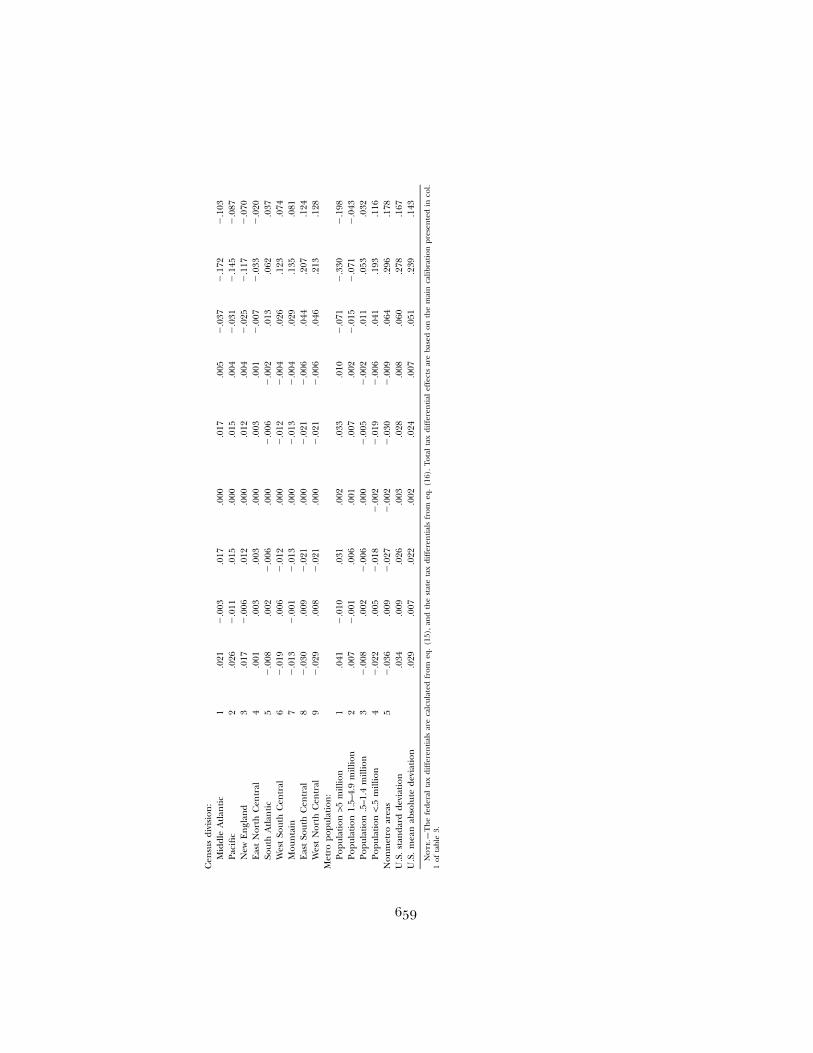
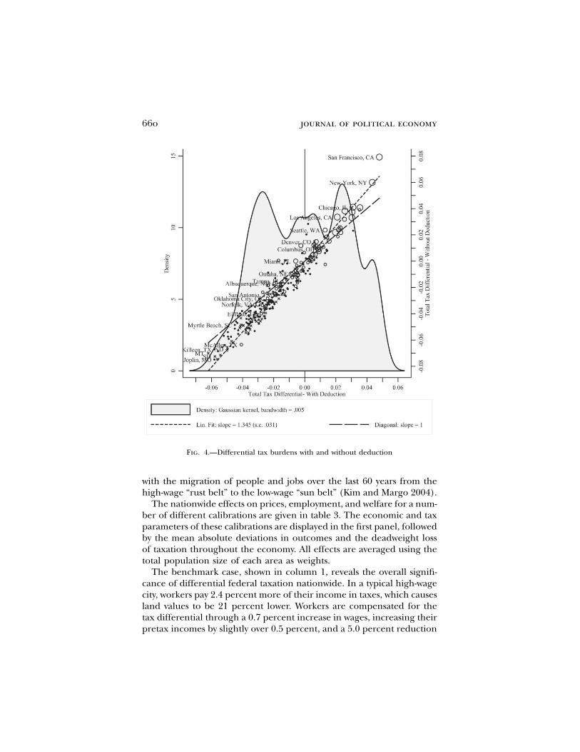
Using the base calibration and estimates of and for 2000, table 2j jˆw preports estimates of tax differentials and their effects across selectedcities, and by census division and metropolitan size.18 The wage anddeduction components of the federal tax differential in (15) are incolumns 1 and 2, with the sum in column 3. State tax differentials arein column 4, and the total combined tax differential is in column 5. Akernel density estimate of these total tax differentials is drawn in figure4.

The unequal distribution of taxes is substantial: the mean absolutedeviation of federal tax differentials equals 2.2 percent of income, andwith state taxes this rises to 2.4 percent. Starting at an average federaltax rate of 17 percent, a worker moving from a typical low-wage city toa typical high-wage city sees her average tax rate rise from 14.8 percentto 19.2 percent, paying 27 percent more in federal taxes. Although taxdifferences are compensated for in local prices, this represents a hor-izontal transfer of $269 billion (in 2008) from workers in high-wageareas to similarly skilled workers in low-wage areas.19

According to the simulation, the tax differential from equation (15)is given numerically by . Tax differences arej j jˆˆdt /m p 0.271w � 0.035pdriven largely by wage differences, although price differences have someeffect. This phenomenon is illustrated in figure 3 by the upward-sloping

17 Weingast, Shepsle, and Johnsen (1981) explain when localized spending should betreated as a transfer.

18 A full list is provided in Albouy (2008b).19 The average federal tax rate of 17 percent includes federal income taxes and payroll

taxes, appropriately adjusted (Congressional Budget Office 2003). Multiplying the meanabsolute deviation of federal tax differentials, 0.221, by personal income in 2008 of $12.11trillion produces a figure of $269 billion. Using GDP produces $317 billion, or adjustedgross income of roughly $189 billion.


average iso-tax line: a city’s federal tax differential is proportional tothe vertical distance of the city marker above this line. Empirically, thedeductions tend to reduce tax differences across areas, as wages andhousing costs are positively related. Figure 4 shows how eliminating thededuction would change the distribution of federal taxes across cities,increasing the tax differential gradient by 34.5 percent. Thus, withoutthe deduction, the average tax differential would be 3.2 percent, makingthe distribution of federal taxes even more unequal.20

Each city’s tax differential depends on its attributes, according to thenumeric analogue of equation (7): j j jˆ ˆdt /m p �0.185Q � 0.228A �X

, which adjusts for deductions and state taxes. Thus, federaljˆ0.025A Y

taxes depend quite positively on a city’s trade productivity and negativelyon quality of life and, to a lesser extent, home productivity. The meanabsolute deviation of is 0.037, whereas the corresponding figure forjQ

, assuming for all , is 0.111. Accordingly, the average taxj jˆ ˆA A p 0 jX Y

differential from quality-of-life differences alone is only 0.7 percent,whereas the same from productivity differences alone would be 2.6 per-cent. Thus, tax differences appear to be caused more by productivitydifferences than by quality-of-life differences. As a result, tax burdensare highest in large, productive cities in the Northeast, Midwest, andPacific, whereas small, less productive towns and nonmetropolitan areas,particularly in the South, receive a large tax break.

The total tax differentials are considerable relative to typical differ-ences in local taxes. Any local official would consider a permanent 3percent tax on local residents without any compensating services to bea fiscal calamity. Yet, central governments are imposing this situationon cities such as Chicago, New York, and San Francisco. However, anunconditional grant of 3 percent of income in perpetuity dwarfs almostany pork-barrel project. Relative to the national average, this is whatworkers in cities such as Norfolk and Tucson, as well as most nonmet-ropolitan areas, effectively receive from the federal government.

These large tax differentials have considerable effects on prices andemployment, seen in the last four columns of table 2. For example, theadditional taxes paid to Washington and Albany by New York City raisewages by 1.3 percent, lower long-run housing costs by 9 percent, andlower land values by 35 percent. The employment effect is especiallystriking, stating that employment is 23 percent lower than in an un-distorted equilibrium. This effect may seem too large, but it may bereasonable in the long run, as sizable federal taxes first affected averageworkers in World War II. The rise of the income tax is certainly consistent

20 Since the existing tax system has a deduction, the tax differentials with no deductionin fig. 4 and col. 6 of table 3 are based on the counterfactual wage without a deduction.Counterfactual wages are simply . The tax differentials with no deductionj j jˆ ˆ ˆw p w � dw0

are similar to the ones for which the deduction is just ignored and is used.jw

658

TA

BL

E2

Tax

Dif

fere

nti

als

and

Th

eir

Eff

ects

on

Pric

esan

dE

mpl

oym

ent,

2000

Fed

eral

Tax

Dif

fere

nti

alTo

tal

Tax

Dif

fere

nti

alE

ffec

ts

Tax

Paym

ent

Ran

k

From

Wag

e(1

)

From

Ded

uct

(2)

Tota

lFe

dera

l(3

)

Stat

eTa

xD

iffe

ren

tial

(4)

Tota

lTa

xD

iffe

ren

tial

(5)

Wag

e(6

)

Hou

sin

gC

ost

(7)

Lan

dR

ent

(8)

Em

ploy

men

t(9

)

Met

roar

ea:

San

Fran

cisc

o,C

A1

.068

�.0

23.0

45.0

04.0

48.0

15�

.103

�.4

80�

.288

New

York

,N

Y2

.054

�.0

13.0

41.0

02.0

43.0

13�

.093

�.4

34�

.261

Det

roit

,M

I3

.035

�.0

03.0

32.0

04.0

36.0

11�

.076

�.3

55�

.213

Har

tfor

d,C

T4

.039

�.0

05.0

35.0

01.0

35.0

11�

.076

�.3

52�

.211

Ch

icag

o,IL

6.0

35�

.007

.029

.003

.031

.009

�.0

67�

.310

�.1

86W

ash

ingt

on,

DC

7.0

34�

.005

.029

.002

.031

.009

�.0

66�

.306

�.1

83Ph

ilade

lph

ia,

PA8

.030

�.0

02.0

28.0

02.0

30.0

09�

.065

�.3

03�

.182

Bos

ton

,M

A9

.035

�.0

11.0

25.0

01.0

26.0

08�

.056

�.2

59�

.155

Min

nea

polis

,M

N10

.023

�.0

02.0

21.0

05.0

26.0

08�

.055

�.2

56�

.154

Los

An

gele

s,C

A15

.033

�.0

12.0

21.0

00.0

21.0

06�

.045

�.2

09�

.126

Jack

son

ville

,FL

114

�.0

19.0

03�

.016

.000

�.0

15�

.005

.033

.153

.092

Okl

ahom

aC

ity,

OK

160

�.0

32.0

06�

.026

.002

�.0

24�

.007

.051

.239

.143

Nor

folk

,VA

188

�.0

28.0

02�

.026

�.0

04�

.030

�.0

09.0

64.3

00.1

80Tu

cson

,A

Z19

5�

.029

.000

�.0

29�

.003

�.0

32�

.010

.069

.322

.193

Kill

een

,T

X24

1�

.060

.007

�.0

53�

.005

�.0

58�

.018

.125

.582

.349

659

Cen

sus

divi

sion

:M

iddl

eA

tlan

tic

1.0

21�

.003

.017

.000

.017

.005

�.0

37�

.172

�.1

03Pa

cifi

c2

.026

�.0

11.0

15.0

00.0

15.0

04�

.031

�.1

45�

.087

New

En

glan

d3

.017

�.0

06.0

12.0

00.0

12.0

04�

.025

�.1

17�

.070

Eas

tN

orth

Cen

tral

4.0

01.0

03.0

03.0

00.0

03.0

01�

.007

�.0

33�

.020

Sout

hA

tlan

tic

5�

.008

.002

�.0

06.0

00�

.006

�.0

02.0

13.0

62.0

37W

est

Sout

hC

entr

al6

�.0

19.0

06�

.012

.000

�.0

12�

.004

.026

.123

.074

Mou

nta

in7

�.0

13�

.001

�.0

13.0

00�

.013

�.0

04.0

29.1

35.0

81E

ast

Sout

hC

entr

al8

�.0

30.0

09�

.021

.000

�.0

21�

.006

.044

.207

.124

Wes

tN

orth

Cen

tral

9�

.029

.008

�.0

21.0

00�

.021

�.0

06.0

46.2

13.1

28M

etro

popu

lati

on:

Popu

lati

on1

5m

illio

n1

.041

�.0

10.0

31.0

02.0

33.0

10�

.071

�.3

30�

.198

Popu

lati

on1.

5–4.

9m

illio

n2

.007

�.0

01.0

06.0

01.0

07.0

02�

.015

�.0

71�

.043

Popu

lati

on.5

–1.4

mill

ion

3�

.008

.002

�.0

06.0

00�

.005

�.0

02.0

11.0

53.0

32Po

pula

tion

!.5

mill

ion

4�

.022

.005

�.0

18�

.002

�.0

19�

.006

.041

.193

.116

Non

met

roar

eas

5�

.036

.009

�.0

27�

.002

�.0

30�

.009

.064

.296

.178

U.S

.st

anda

rdde

viat

ion

.034

.009

.026

.003

.028

.008

.060

.278

.167

U.S

.m

ean

abso

lute

devi

atio

n.0

29.0

07.0

22.0

02.0

24.0

07.0

51.2

39.1

43

No

te.—

Th

efe

dera

lta

xdi

ffer

enti

als

are

calc

ulat

edfr

omeq

.(1

5),

and

the

stat

eta

xdi

ffer

enti

als

from

eq.

(16)

.To

tal

tax

diff

eren

tial

effe

cts

are

base

don

the

mai

nca

libra

tion

pres

ente

din

col.

1of

tabl

e3.


Fig. 4.—Differential tax burdens with and without deduction

with the migration of people and jobs over the last 60 years from thehigh-wage “rust belt” to the low-wage “sun belt” (Kim and Margo 2004).

The nationwide effects on prices, employment, and welfare for a num-ber of different calibrations are given in table 3. The economic and taxparameters of these calibrations are displayed in the first panel, followedby the mean absolute deviations in outcomes and the deadweight lossof taxation throughout the economy. All effects are averaged using thetotal population size of each area as weights.

The benchmark case, shown in column 1, reveals the overall signifi-cance of differential federal taxation nationwide. In a typical high-wagecity, workers pay 2.4 percent more of their income in taxes, which causesland values to be 21 percent lower. Workers are compensated for thetax differential through a 0.7 percent increase in wages, increasing theirpretax incomes by slightly over 0.5 percent, and a 5.0 percent reduction

TA

BL

E3

Sim

ula

ted

Eff

ects

of

Tax

Dif

fere

nti

als

acro

ssA

llA

reas

for

Alt

ern

ate

Cal

ibra

tio

ns

Ben

chm

ark

Cas

e(1

)

All

Lan

din

Hom

eG

oods

(2)

Smal

ler

Lan

dSh

are

(3)

Lar

ger

Em

ploy

men

tR

espo

nse

:C

obb-

Dou

glas

(4)

Wag

eD

iffe

ren

tial

sTw

o-T

hir

dsE

stim

ated

Size

(5)

Hou

sin

gD

educ

tion

sE

limin

ated

(6)

Fede

ral

Taxe

sO

nly

,N

oSt

ate

Taxe

s(7

)

Add

ing

Fede

ral

Spen

din

gD

iffe

ren

ces

(8)

Eco

nom

icpa

ram

eter

s:H

ome-

good

ssh

are,

s y.3

60.3

60.3

60.3

60.3

60.3

60.3

60.3

60Tr

aded

-goo

dla

nd

shar

e,v L

.025

.000

.013

.025

.025

.025

.025

.025

Trad

ed-g

ood

labo

rsh

are,

v N.8

25.8

50.8

25.8

25.8

25.8

25.8

25.8

25H

ome-

good

lan

dsh

are,

fL

.233

.278

.117

.233

.233

.233

.233

.233

Hom

e-go

odla

bor

shar

e,f

N.6

17.5

72.6

17.6

17.6

17.6

17.6

17.6

17E

last

icit

yof

empl

oym

ent

tota

x/in

com

e,�

�6.

000

�6.

000

�6.

000

�9.

370

�6.

000

�6.

000

�6.

000

�6.

000

Impl

ied

shar

eof

inco

me

tola

nd,

s R.1

00.1

00.0

50.1

00.1

00.1

00.1

00.1

00Ta

xpa

ram

eter

s:M

argi

nal

tax

rate

,t�

.361

.361

.361

.361

.361

.361

.333

.361

Ded

ucti

onle

vel,

d.2

91.2

91.2

91.2

91.2

91.0

00.2

57.2

91A

vera

gepe

rcen

tef

fect

s(m

ean

abs.

dev.

):Ta

xdi

ffer

enti

al,

jEF

dtF

.024

.024

.024

.024

.014

.032

.022

.027

Wag

eef

fect

,j

ÊF

dwF

.007

.000

.007

.007

.004

.010

.007

.008

Hom

e-go

odpr

ice

effe

ct,

j ÊF

dpF

.051

.066

.051

.051

.029

.069

.048

.059

Lan

dre

nt

effe

ct,

j ÊF

drF

.239

.239

.478

.239

.136

.323

.222

.274

Em

ploy

men

tef

fect

,j

ÊF

dNF

.143

.143

.143

.224

.082

.194

.133

.164

Dea

dwei

ght

loss

from

loca

tion

alin

effi

cien

cy:

As

ape

rcen

tof

inco

me,

TO

TD

WL

/(m

N)

.23%

.23%

.23%

.36%

.07%

.43%

.20%

.31%

Tota

l,bi

llion

spe

rye

ar,

2008

dolla

rs28

2828

449

5224

37Pe

rca

pita

per

year

,20

08do

llars

9393

9314

630

174

8212

4

No

te.—

Wag

e,la

nd

ren

t,h

ome-

good

pric

e,an

dem

ploy

men

tef

fect

sar

eca

lcul

ated

from

eqq.

(5),

(8a)

,(8b

),an

d(1

0).D

eadw

eigh

tlo

ssis

dete

rmin

edfr

omeq

.(11

),an

dth

edo

llar

valu

esar

eba

sed

ona

pers

onal

inco

me

mea

sure

of$1

2.11

billi

on.

Th

eC

obb-

Dou

glas

elas

tici

tyof

empl

oym

ent

isde

rive

din

onlin

eA

pps.

Aan

dB

.Se

ete

xtfo

rfu

rth

erde

tail.


in the housing prices, reflecting a cost-of-living reduction of 1.8 percent.Thus, workers are compensated for higher taxes more through lowercosts than through higher wages.

The negative employment effect on a typical high-wage city is 14percent. Taken together, the employment effects create a substantialdeadweight loss of about 0.23 percent of income a year, or $28 billionin 2008. As these numbers are based on a calibrated model, they shouldnot be taken as absolute truth, but they do provide a sense of themagnitude of the impacts and costs caused by the unequal distributionof federal taxes.21

Alternative calibrations in table 3 are shown in columns to the right.In column 2, all land is devoted to home-good production, keeping thetotal share of income to land constant: in this case, wage differentialsare unaffected by taxes, whereas home-good price differentials are af-fected more. In column 3, the cost shares of land in both sectors arereduced by one-half, with mobile capital taking up the remaining costs;this doubles the impact on land rents without changing any of the otherquantities.

Column 4 shows that if is �9.37, which corresponds to when pro-�duction and preferences are Cobb-Douglas, the employment effects anddeadweight loss are increased proportionally. Column 5 cuts wage dif-ferentials down to two-thirds their original size, in case unobserved se-lection makes the estimated differentials too large: this lowers the dif-ferential taxes and price and employment effects by 41 percent andreduces the deadweight loss to only 0.07 percent of income. Column 6reveals that if the deduction is eliminated but tax rates on labor areheld constant, then the tax effects would become 35 percent larger andthe deadweight loss would increase to 0.43 percent of income. Finally,column 7 looks at the effect of federal taxes only, ignoring state taxes.Since federal taxes account for 92 percent of tax differences, the effectsare only slightly smaller.

D. The Distribution of Federal Spending

The unequal burden of federal taxation would be much less of an issueif it was compensated for by federal spending differences. To explorethis possibility, table 4 reports coefficients from regressions of spendingdifferentials, both raw and adjusted, on tax differentials in 2000. In theraw differentials, there is a positive correlation with federal purchases

21 In the base calibration, agglomeration effects could dampen the positive effect oftaxes on wages. According to Rosenthal and Strange (2004), the elasticity of wages withrespect to population size due to agglomeration is close to 4 percent. At this level, a 17percent reduction in employment from taxes reduces wages by 0.7 percent, which wouldoffset the 0.7 percent predicted increase in wages due to higher land-to-labor ratios.


TABLE 4Differential Federal Spending Patterns Relative to Differential

Taxation Patterns, 2000

Type of Federal Spending

AllSpending

(1)

Wages andContracts

(2)

NonworkerBenefits

(3)

All OtherSpending

(4)

A. Raw spending differentials:federal tax differential �.134 .305 �.261 �.025

(.212) (.158) (.092) (.070)B. Adjusted spending differentials:

federal tax differential �.246 �.094 �.032 �.098(.157) (.095) (.025) (.037)

Note.—Each entry corresponds to a separate regression, reporting the coefficient on the federal tax differentialvariable using alternate measures of federal spending as the dependent variable. Regressions weighted by populationfor all 290 observations. Robust standard are errors reported in parentheses. Adjusted spending differentials controlfor socioeconomic disparities as described in online App. C.

(wages and contracts), a negative correlation with nonworker benefits,and no correlation with other spending, the category closest to a lo-cational transfer. Once population characteristics are controlled for,correlations for wages and contracts and nonworker benefits becomenegative and insignificant, while other spending, as well as aggregatespending, becomes negatively correlated with federal tax differentials.Although the federal government makes greater purchases in areas withhigher wages, this arises from its need to purchase skilled labor.

Figure 5, which graphs “other spending” differentials against tax dif-ferentials, makes it clear that federal spending does not offset differ-ences in federal taxation and may in fact do the opposite. Column 8of table 3 simulates the effects of tax differentials net of other spending:these differentials have slightly larger variance, increasing the tax effectsand deadweight loss by a small amount.

VII. Conclusion

Any tax on labor income creates an incentive for workers to leave high-wage areas in favor of low-wage areas. Although mobile workers shouldbe compensated for the resulting tax differences through adjustmentsin local prices and wages, the resulting geographic distribution of em-ployment will be distorted, causing a substantial welfare loss.

The simulated effects of federal taxes on prices, employment, andwelfare are based on the assumption that city attributes are unaffectedby population movements. When city attributes are affected by popu-lation size, these effects could be smaller or larger than predicted. Fur-thermore, the distribution of city sizes may no longer be optimal evenin the absence of federal taxes, which could ameliorate or aggravatepreexisting distortions. Given the complexities of dealing with endog-


Fig. 5.—Federal spending and tax differentials across areas

enous attributes, these issues are left for further work (see Albouy andSeegert 2009).

Politicians who represent high-wage areas may legitimately complainthat their districts pay a disproportionate share of federal taxes. How-ever, in most countries, reforms to equalize the federal tax burden acrossareas would likely meet fierce political opposition. In the United States,highly taxed areas tend to be in large cities inside of populous states,which have low congressional representation per capita, making theprospect of reform daunting. In other countries, such as Canada, ruralareas also receive disproportionate representation in national legisla-tures. Nevertheless, when considering federal tax reforms, policy makersshould be aware of their spatial consequences on local prices, employ-ment, and welfare.


References

Albouy, David. 2008a. “Are Big Cities Really Bad Places to Live? Improving Qual-ity-of-Life Estimates across Cities.” Working Paper no. 14472 (November),NBER, Cambridge, MA.

———. 2008b. “The Unequal Geographic Burden of Federal Taxation.” WorkingPaper no. 13995 (May), NBER, Cambridge, MA.

———. 2009. “What Are Cities Worth? Land Rents, Local Productivity, and theCapitalization of Amenity Values.” Working Paper no. 14981 (May), NBER,Cambridge, MA.

Albouy, David, and Nathan Seegert. 2009. “The Optimal Distribution of Popu-lation across Cities and the Private-Social Wedge.” Manuscript, Univ. Michigan.

Antras, Pol. 2004. “Is the U.S. Aggregate Production Function Cobb-Douglas?New Estimates of the Elasticity of Substitution.” Contributions to Macroeconomics4 (1): 1–33.

Bartik, Timothy J. 1991. Who Benefits from State and Local Economic DevelopmentPolicies? Kalamazoo, MI: Upjohn Inst.

Beeson, Patricia E., and Randall W. Eberts. 1989. “Identifying Productivity andAmenity Effects in Interurban Wage Differentials.” Rev. Econ. and Statis. 71(August): 443–52.

Berndt, Ernst. 1976. “Reconciling Alternative Estimates of the Elasticity of Sub-stitution.” Rev. Econ. and Statis. 58 (February): 59–68.

Blanchard, Olivier-Jean, and Lawrence F. Katz. 1992. “Regional Evolutions.”Brookings Papers Econ. Activity (1): 1–61.

Boskin, Michael J., Laurence J. Kotlikoff, Douglas J. Puffert, and John B. Shoven.1987. “Social Security: A Financial Appraisal across and within Generations.”Nat. Tax J. 40 (March): 19–34.

Brady, Peter, Julie-Anne Cronin, and Scott Houser. 2003. “Regional Differencesin the Utilization of the Mortgage Interest Deduction.” Public Finance Rev. 31(July): 327–66.

Bureau of Labor Statistics. 2002. Consumer Expenditures in 2000. Washington, DC:Government Printing Office.

Cassimatis, Peter J. 1969. Economics of the Construction Industry. New York: NationalIndus. Conf. Bd.

Congressional Budget Office. 2003. Effective Federal Tax Rates, 1997 to 2000. Wash-ington, DC: Government Printing Office.

———. 2005. Effective Marginal Tax Rates on Labor Income. Washington, DC: Gov-ernment Printing Office.

Davis, Morris A., and Jonathan Heathcoate. 2007. “The Price and Quantity ofResidential Land in the United States.” J. Monetary Econ. 54 (November): 2595–2620.

Dubay, Curtis S. 2006. “Federal Tax Burdens and Expenditures by State: WhichStates Gain Most from Federal Fiscal Operations.” Special Report no. 139, TaxFound., Washington, DC.

Feenberg, Daniel, and Elisabeth Coutts. 1993. “An Introduction to the TAXSIMModel.” J. Policy Analysis and Management 12 (Winter): 189–94.

Feenberg, Daniel R., Andrew W. Mitrusi, and James M. Poterba. 1997. “Distri-butional Effects of Adopting a National Retail Sales Tax.” Working Paper no.5885 (November), NBER, Cambridge, MA.

Gladwell, Malcolm. 1996. “U.S. to New York: It’s Still Dutch Treat.” WashingtonPost, March 7.

Glaeser, Edward L. 1998. “Should Transfer Payments Be Indexed to Local PriceLevels?” Regional Sci. and Urban Econ. 28 (January): 1–20.


Glaeser, Edward L., and David Mare. 2001. “Cities and Skills.” J. Labor Econ. 19(April): 316–42.

Glaeser, Edward L., and Jesse M. Shapiro. 2003. “The Benefits of the HomeMortgage Interest Deduction.” In Tax Policy and the Economy, vol. 17, editedby James M. Poterba. Cambridge, MA: MIT Press.

Goodman, Allen C. 1988. “An Econometric Model of Housing Price, PermanentIncome, Tenure Choice, and Housing Demand.” J. Urban Econ. 23 (May): 327–53.

Gyourko, Joseph, and Todd Sinai. 2003. “The Spatial Distribution of Housing-Related Ordinary Tax Benefits.” Real Estate Econ. 31 (4): 527–75.

———. 2004. “The (Un)Changing Geographical Distribution of Housing TaxBenefits: 1980 to 2000.” In Tax Policy and the Economy, vol. 18, edited by JamesM. Poterba. Cambridge, MA: MIT Press.

Gyourko, Joseph, and Joseph Tracy. 1989. “The Importance of Local Fiscal Con-ditions in Analyzing Local Labor Markets.” J.P.E. 97 (October): 1208–31.

———. 1991. “The Structure of Local Public Finance and the Quality of Life.”J.P.E. 99 (August): 774–806.

Harberger, Arnold C. 1962. “The Incidence of the Corporate Income Tax.” J.P.E.70 (1962): 215–40.

———. 1964. “Principles of Efficiency: The Measurement of Waste.” A.E.R. Papersand Proc. 54 (May): 58–76.

Hoffman, David K., and J. Scott Moody. 2003. “Federal Income Taxes and theCost of Living: States with Lower Cost of Living Enjoy Great Federal TaxAdvantage.” Special Report no. 125, Tax Found., Washington, DC.

Ioannides, Yannis M., and Jeffrey E. Zabel. 2003. “Neighborhood Effects andHousing Demand.” J. Appl. Econometrics 18 (September): 563–84.

Jones, Ronald W. 1965. “The Structure of Simple General Equilibrium Models.”J.P.E. 73 (December): 557–72.

Kaplow, Louis. 1995. “Regional Cost-of-Living Adjustments in Tax/TransferSchemes.” Tax Law Rev. 51 (Winter): 175–98.

———. 1996. “Fiscal Federalism and the Deductibility of State and Local Taxesunder the Federal Income Tax.” Virginia Law Rev. 82 (April): 413–92.

Keiper, Joseph S., Ernest Kurnow, Clifford D. Clark, and Harvey H. Segal. 1961.Theory and Measurement of Rent. Philadelphia: Chilton.

Kim, Sukkoo, and Robert Margo. 2004. “Historical Perspectives on U.S. Eco-nomic Geography.” In Handbook of Regional and Urban Economics, vol. 4, editedby J. V. Henderson and J.-F. Thisse. Amsterdam: North-Holland.

Knoll, Michael S., and Thomas D. Griffith. 2003. “Taxing Sunny Days: AdjustingTaxes for Regional Living Costs and Amenities.” Harvard Law Rev. 116 (Feb-ruary): 987–1023.

Kotlikoff, Laurence J., and Lawrence H. Summers. 1987. “Tax Incidence.” InHandbook of Public Economics, vol. 2, edited by A. J. Auerbach and M. Feldstein.Amsterdam: North-Holland.

Krueger, Alan B. 1999. “Measuring Labor’s Share.” A.E.R. Papers and Proc. 89(May): 45–51.

Lucas, Robert E. 1969. “Labor-Capital Substitution in U.S. Manufacturing.” InThe Taxation of Income from Capital, edited by Arnold Harberger and Martin J.Bailey. Washington, DC: Brookings Inst.

Malpezzi, Stephen, Gregory H. Chun, and Richard K. Green. 1998. “New Place-to-Place Housing Price Indexes for U.S. Metropolitan Areas, and Their De-terminants.” Real Estate Econ. 26 (June): 235–74.


McDonald, John F. 1981. “Capital-Land Substitution in Urban Housing: A Surveyof Empirical Estimates.” J. Urban Econ. 9 (March): 190–211.

Mieszkowski, Peter. 1972. “The Property Tax: An Excise Tax or a Profits Tax?”J. Public Econ. 1 (April): 73–96.

Moretti, Enrico. 2008. “Real Wage Inequality.” Working Paper no. 14370 (No-vember), NBER, Cambridge, MA.

Moynihan, Daniel Patrick. 2000. “Introduction.” In The Federal Budget and theStates: Fiscal Year 1999. Washington, DC: Taubman Center for State and LocalGovernment, John F. Kennedy School of Government, U.S. Senate PrintingOffice.

Phillips, Joseph M., and Ernest P. Goss. 1995. “The Effect of State and LocalTaxes on Economic Development: A Meta-analysis.” Southern Econ. J. 62 (Oc-tober): 320–33.

Poterba, James M. 1992. “Taxation and Housing: Old Questions, New Answers.”A.E.R. Papers and Proc. 82 (May): 237–42.

———. 1998. “The Rate of Return to Corporate Capital and Factor Shares: NewEstimates Using Revised National Income Accounts and Capital Stock Data.”Carnegie-Rochester Conf. Series Public Policy 48:211–46.

Rappaport, Jordan. 2008. “A Productivity Model of City Crowdedness.” J. UrbanEcon. 63 (March): 715–22.

Roback, Jennifer. 1980. “The Value of Local Urban Amenities: Theory and Mea-surement.” PhD diss., Univ. Rochester.

———. 1982. “Wages, Rents, and the Quality of Life.” J.P.E. 90 (December):1257–78.

Rosen, Harvey. 1985. “Housing Subsidies: Effects on Housing Decisions, Effi-ciency, and Equity.” In Handbook of Public Economics, vol. 1, edited by M. Feld-stein and A. Auerbach. Amsterdam: North-Holland.

Rosen, Sherwin. 1979. “Wages-Based Indexes of Urban Quality of Life.” In CurrentIssues in Urban Economics, edited by P. Mieszkowski and M. Straszheim. Balti-more: Johns Hopkins Univ. Press.

Rosenthal, Stuart, and William Strange. 2004. “Evidence on the Nature andSources of Agglomeration Economies.” In Handbook of Regional and UrbanEconomics, vol. 4, edited by J. V. Henderson and J.-F. Thisse. Amsterdam: North-Holland.

Ruggles, Steven, et al. 2004. Integrated Public Use Microdata Series: Version 3.0.Minneapolis: Minnesota Population Center.

Shapiro, Jesse M. 2006. “Smart Cities: Quality of Life, Productivity, and theGrowth Effects of Human Capital.” Rev. Econ. and Statis. 88 (May): 324–35.

Sieg, Holger, Dennis Epple, and Brett Gordon. Forthcoming. “A New Approachto Estimating the Production Function for Housing.” A.E.R.

Thorsnes, Paul. 1997. “Consistent Estimates of the Elasticity of Substitution be-tween Land and Non-land Inputs in the Production of Housing.” J. UrbanEcon. 42 (July): 98–108.

Tiebout, Charles M. 1956. “A Pure Theory of Local Expenditures.” J.P.E. 64(October): 416–24.

Valentinyi, Akos, and Berthold Herrendorf. 2008. “Measuring Factor IncomeShares at the Sectoral Level.” Rev. Econ. Dynamics 11 (October): 820–35.

Weingast, Barry R., Kenneth A. Shepsle, and Christopher Johnsen. 1981. “ThePolitical Economy of Benefits and Costs: A Neoclassical Approach to Distrib-utive Politics.” J.P.E. 89 (August): 642–64.

Wildasin, David E. 1980. “Locational Efficiency in a Federal System.” RegionalSci. and Urban Econ. 10 (November): 453–71.

the unequal geographic burden of federal taxationdavidalbouy.net/federaltaxes.pdf · federal tax...

Documents