the universality class of the electroweak theory · ddepartment of physics, p.o.box 9, 00014...
TRANSCRIPT

CERN-TH/98-08NORDITA-98/30HE
hep-lat/9805013
THE UNIVERSALITY CLASS OF THE ELECTROWEAK THEORY
K. Rummukainena1, M. Tsypinb2, K. Kajantiec,d3, M. Lainec,d4,and M. Shaposhnikovc5
aNordita, Blegdamsvej 17, DK-2100 Copenhagen, Denmark
bDepartment of Theoretical Physics, Lebedev Physical Institute,117924 Moscow, Russia
cTheory Division, CERN, CH-1211 Geneva 23, Switzerland
dDepartment of Physics, P.O.Box 9, 00014 University of Helsinki, Finland
Abstract
We study the universality class and critical properties of the electroweak theory atfinite temperature. Such critical behaviour is found near the endpoint mH = mH,c
of the line of first order electroweak phase transitions in a wide class of theories, in-cluding the Standard Model (SM) and a part of the parameter space of the MinimalSypersymmetric Standard Model (MSSM). We find that the location of the endpointcorresponds to the Higgs mass mH,c = 72(2) GeV in the SM with sin2 θW = 0, andmH,c < 80 GeV with sin2 θW = 0.23. As experimentally mH > 88 GeV, there is noelectroweak phase transition in the SM. We compute the corresponding critical indicesand provide strong evidence that the phase transitions near the endpoint fall into thethree dimensional Ising universality class.
CERN-TH/98-08NORDITA-98/30HEMay 1998

1 Introduction
The finite temperature phase transition in the Standard Model (SM) is known to be afirst order transition for small and a crossover for large Higgs masses [1]. In betweenthere is a critical region at about mH = 75 GeV [2, 3] (see also [4]). The purpose ofthis paper is to study this critical region in a detailed manner. We shall show that theuniversality class of the endpoint is that of the three-dimensional (3d) Ising model. Wealso obtain the value mH,c < 80 GeV for the endpoint Higgs mass in the SM. Giventhat the experimental 95% C.L. lower limit is mH > 87.9 GeV [5], there would be nophase transition, only a crossover, if the physics were that of the SM.
Universality implies a tremendous simplification in the degrees of freedom of the sys-tem. Here the first step is the removal of all fermionic and all non-static (not constantin imaginary time) bosonic fields [6]. Equivalently, one integrates out all fields withmasses >∼πT . This works for equilibrium phenomena in the high T small coupling limit.Furthermore, all masses ∼ gT can also be integrated out. Hereby one obtains a 3deffective theory S[Bi, A
ai , φk], i, a = 1, 2, 3, k = 1, . . . , 4, with SU(2)×U(1) symmetry
and a fundamental doublet φ [7]. The superrenormalizable 3d theory provides a verygood approximation to high T 4d physics. The accuracy of the effective descriptionhas been discussed in detail in [7]; further corrections to the effective action can alsobe computed.
The previous steps can be performed perturbatively, but further progress is onlypossible with numerical lattice Monte Carlo techniques (for reviews, see [8, 9]). Interms of SM physics, these show the existence of a line of first order phase transitionsTc = Tc(mH), mH < mH,c, which ends at Tc(mH,c) and turns into a crossover atmH > mH,c. When approaching the endpoint along the first order line, the mass of oneof the scalar excitations seems to go to zero suggesting [10] that ultimately all othermasses could be integrated out, leaving near (mH,c, Tc(mH,c)) a final effective theoryScrit[φ
′] containing only one scalar degree of freedom φ′.To be more precise, the electroweak theory with a Higgs doublet contains a massless
vector excitation, corresponding to the hypercharge field high in the symmetric phaseand to the photon deep in the Higgs phase. The fact that this state is massless atany temperature ensures the “topological” similarity of the phase diagrams of theSU(2)+Higgs and SU(2)×U(1)+Higgs theories [11]. Moreover, the lowest order gauge-invariant coupling of a real scalar to a vector field φ′FijFij has a dimensionality greaterthan 3, and thus the scalar is decoupled from the massless vector in the infrared. Hence,for discussing the universal properties of the theory near the endpoint, we can workwith the SU(2)+Higgs theory S[Aai , φk], disregarding the U(1) interactions. We shall inthe following show that the endpoint of this theory belongs to the 3d Ising universalityclass [12, 13]. The universality class of the 3d O(4) invariant spin model [14, 15], whichhas also been proposed as a possible candidate [16], can be ruled out.
The matching of the continuum theories S[Aai , φk]→ Scrit[φ′] is a delicate issue and
1

at this stage we do not determine the couplings of Scrit, only its universality class. Wefirst discretize the continuum theory at fixed lattice spacing a and determine the criticalproperties of the discretized theory near the endpoint (mH,c, Tc(mH,c)). This is doneby studying the properties of probability distributions of various observables (hoppingterm, (φ2 − 1)2, etc) averaged over a finite-volume system (we consider the theoryin a cubic box with periodic boundary conditions). We obtain the joint probabilitydistribution of up to 6 observables and analyze it in two ways:
1. We compute the fluctuation matrix, study the dependence of its eigenvalues onthe volume and obtain critical indices, which turn out to be consistent with those ofthe 3d Ising model,
2. We show that for a certain pair of observables, which may be denoted as M-likeand E-like, the joint probability distribution has a very nontrivial form which matchesclosely the joint distribution of magnetization M and energy E of the 3d Ising modelin a box of the same geometry. This guarantees that not only the critical indices, butalso higher moments agree with those of the 3d Ising model. As a byproduct we obtainthe mapping of the 6-dimensional operator space to the Ising model. This is a fixedlattice spacing version of the critical mapping: S6[Aai , φk, a]→ SIsing.
Our method has much in common with, and can be considered as the generalizationof, the method used by Alonso et al [17] to locate and study the endpoint of the firstorder transition line separating the Higgs and confinement phases in the 4d U(1)+Higgsmodel, and the method developed by Bruce and Wilding [18] for the study of theliquid-gas critical point, both of which rely on considering two-dimensional probabilitydistributions and finding the M-like and E-like directions. However, our method aswell as some aspects of the critical behaviour of our system, differ in many importantrespects from those in [17, 18].
Finally, an extrapolation to a→ 0 will have to be made. There is no change in theuniversal properties. However, this extrapolation is needed to get the continuum valueof the (non-universal) quantity mH,c. As mentioned above, this in conjunction with theexperimental lower limit implies that the critical region of the 3d effective theory canonly be physically relevant in a beyond-the-SM electroweak theory, such as the MSSM.
The plan of the paper is the following. We formulate the problem in Sec. 2 in somemore detail, and outline its solution in Sec. 3. In Sec. 4 we review the basic properties ofO(N) spin models. Sec. 5 contains a detailed presentation of the method of determiningthe universality class of the 3d SU(2)+Higgs theory. Asymmetry effects are studied inSec. 6. In Sec. 7 we summarize the results for the critical properties and for mH,c, andwe conclude in Sec. 8.
2

2 Formulation of the problem
At finite temperatures, the static bosonic correlators in the Standard Model and manyof its extensions can be derived from the 3d effective action (as discussed above, weomit the U(1) interactions)
S =∫d3x
[1
2TrFijFij + (Diφ)†(Diφ) +m2
3φ†φ+ λ3(φ†φ)2
], (1)
in standard notation. This is a continuum field theory characterized by the dimension-ful gauge coupling g2
3 and by the dimensionless ratios
x = λ3/g23, y = m2
3(g23)/g4
3, (2)
where m23(µ) is the renormalized mass parameter in the MS scheme. The relations
of g23, x, y to the full theory are computable in perturbation theory, and the relative
accuracy thus obtained for non-vanishing one-particle irreducible Green’s functions Gthat conserve parity, C and CP is [7]
δG
G<∼O(g3), (3)
where δG is the error in G. The fact that there is a suppression of error arises from theratio of the scales left and integrated out, O(gT/T ), O(g2T/gT ), and the third powerfrom the types of higher order operators that have been neglected [7]. Hence, for smallcoupling, the physics of the 4d theory can be described accurately with a much simpler3d theory. Explicit derivations have been given in [7, 19].
Instead of using the MS scheme, the 3d continuum theory of Eq. (1) can as well beregulated by using a lattice with the lattice constant a. The action then is
S = βG∑x
∑i<j
(1−1
2TrPij)
− βH∑x
∑i
1
2Tr Φ†(x)Ui(x)Φ(x + i)
+∑x
1
2Tr Φ†(x)Φ(x) + βR
∑x
[1
2Tr Φ†(x)Φ(x)− 1]2 (4)
≡ SG + Shopping + Sφ2 + S(φ2−1)2 ,
in standard notation [Φ is the matrix Φ = (iσ2φ∗, φ)]. The two actions in Eqs. (1),
(4) give the same physics in the continuum limit a → 0 if the three dimensionlessparameters βG, βH , βR in Eq. (4) are related to the three dimensionless parametersg2
3a, x, y in Eq. (1) by the following equations [20]:
βG =4
g23a, (5)
3

βR =β2H
βGx, (6)
y =β2G
8
(1
βH− 3−
2xβHβG
)+
3ΣβG32π
(1 + 4x)
+1
16π2
[(51
16+ 9x− 12x2
)(ln
3βG2
+ ζ)
+ 4.9941 + 5.2153x], (7)
where Σ = 3.1759115 and ζ = 0.08849(1). The two numbers 4.9941 and 5.2153 arespecific for the SU(2)+Higgs theory.
The approach to the continuum limit can be accelerated by removing the O(a) errorsanalytically [21]. For g2
3, x, this can be achieved by reinterpreting the simulation resultsemploying Eqs. (5), (6) as corresponding to
4
(g23)improveda
=4
g23a− 0.6674, (8)
ximproved = x−1
βG(0.018246 + 0.195709x+ 0.583880x2). (9)
For y the issue is more involved, see [21].The phase structure of the theory in Eq. (1) is shown in Fig. 1. There is a first order
line y = yc(x) for x < xc; for x > xc there is only a crossover. The first order lineis localised by using the lattice action in Eq. (4) at some finite lattice spacing a andsystem volume V , finding a two-peak distribution in the measurements of any gaugeinvariant observables and performing the limits V →∞ and a→ 0. At small x� xcthe two peaks are very asymmetric and well separated, signalling a strong transition.When x approaches xc, the two peaks become more symmetric and approach eachother. One of the masses, m0++ measured by the correlator of Φ†Φ, becomes smallerthan the other masses. One expects that m0++ → 0 at xc so that the transition is ofthe second order there.
In practice, one takes the lattice theory in Eq. (4) at some fixed βG and finds thelocation of the first order line in the plane of the remaining two parameters (βH , βR).To approach the continuum limit, one has to repeat the study at higher values of βG(we have used βG = 5, 8 and 12).
Since the mass m0++ is expected to vanish at the endpoint xc, a natural questionarising is whether the effective theory in Eq. (1) could be further reduced leaving onlythe lightest excitations in the final action [22, 23, 10]. Knowing the effective theorywould also imply knowledge of the universality class of the second order transitionat xc. Unfortunately, no systematic perturbative derivation of such an effective actionhas been found. One problem is that in perturbation theory the vector excitations aremassless in the symmetric phase, leading to IR-problems, whereas non-perturbativelythey are massive and are to be integrated out. Thus the construction of the effectivetheory has to be non-perturbative.
4

0.00 0.05 0.10 0.15x
-0.004
-0.002
0.000
0.002
xyc
xI
-0.002
0.000
0.002
x IyIc
Figure 1: Left: The phase diagram of the 3d SU(2)+Higgs theory. The datapoints arefrom [10] and from this paper. The value of x · yc at x → 0 is given by the 1-loopeffective potential and is hence known analytically. Right: The phase diagram of the3d scalar φ4 theory in Eq. (10). The value of xI at the endpoint has to our knowledgenot been determined. The number 0.002 on the vertical axis is symbolic, as the figureis scale invariant in this direction.
As to the functional form of the effective theory, the fact that there is only one lightphysical scalar degree of freedom, the Higgs particle, naturally leads to the suggestion[1, 10] that the corresponding MS continuum effective field theory is
S =∫d3x
[1
2∂iφ∂iφ+ hIφ+
1
2m2Iφ
2 +1
4λIφ
4]. (10)
We discuss the renormalisation and discretization of this theory in the Appendix. Thetheory in Eq. (10) is characterized by the scale λI and by the dimensionless ratios yI =
hI/λ5/2I , xI = m2
I(λI)/λ2I , where m2
I(µ) = −6λ2I/(16π2) log(Λm/µ) is the running mass
parameter in the MS scheme, and Λm is scale invariant. An otherwise possible cubicterm can always be shifted away and this makes hI scale independent. Higher orderoperators could also exist, but they give contributions suppressed by O(m0++/mW )where mW stands for all masses, like the inverse vector correlation length, which remainfinite at xc.
In the critical region the theory in Eq. (10) is in the same universality class as the3d Ising model in an external magnetic field h,
Z =∑{si}
exp[β∑〈ij〉
sisj + h∑i
si], si = ±1. (11)
5

Here β is the inverse temperature, the spins si are located at the sites of a simple cubiclattice, and 〈ij〉 denotes the pairs of nearest neighbours.
To be more specific about constructing an effective theory such as the one in Eq. (10)(or, for a finite lattice spacing, the one in Eq. (11)), there are two questions to beconsidered:
1. Which is the functional form (the degrees of freedom; the symmetries; the uni-versality class) of the effective theory?
2. Which is the mapping between the parameters g23, x, y of the original theory, and
those of the effective theory (such as λI , xI , yI of the scalar theory)?The latter of the two questions is much more difficult than the former one and its
solution will not be attempted here. The reason for the difficulty is that the mappingis non-universal and depends on the detailed UV-properties of the original theory. Inparticular, since the mapping has to be done non-perturbatively on the lattice,
(a) there are finite lattice spacing effects in the lattice formulation in Eq. (4) of theoriginal theory in Eq. (1). These should be identified and removed by an extrapolationto the continuum limit.
(b) there are finite lattice spacing effects in the lattice formulation in Eq. (35) of theeffective theory in Eq. (10). These should be controlled in a similar way.
(c) apart from the lattice spacing effects, there are also higher order operators inthe effective theory in Eq. (10) applying in the continuum limit, due to the degreesof freedom which have been integrated out. The effects of these are suppressed byO(m0++/mW ), but they induce errors immediately when one goes away from the criticalpoint (or is at a finite volume).
For the determination of the universality class, in contrast, none of these problemsarises. By definition, the universal properties are insensitive to the UV. Hence noextrapolation is needed to overcome (a), and a single finite lattice spacing may beused. However, there is a price to be paid for a finite lattice spacing, which is thatthere are infinitely many gauge-invariant operators available, and to find the optimalprojections on the critical directions, one should take as large an operator basis aspossible. No extrapolation to a → 0 is needed for (b), either, and one can directlycompare with the known properties of the spin models in the same universality classas the continuum theory considered. Finally, the non-universal errors responsible for(c) vanish at the critical point (but may induce corrections to scaling, etc). In thefollowing we shall mostly concentrate on the universal properties.
3 Outline of the solution of the problem
To study whether the universality properties of the theory in Eq. (1) match those ofthe scalar theory in Eq. (10), it is sufficient to compare the critical properties of thelattice SU(2)+Higgs theory in Eq. (4) directly with those of the Ising model, Eq. (11).
6

To gain insight into what is happening at the critical point, it is very helpful toconsider two-dimensional probability distributions (joint distributions of two observ-ables) [17, 18]. The motivation is as follows. In the theory in Eq. (4) we have a two-dimensional parameter plane where we find a first order phase transition line whichends in a critical point. In this respect, our system is very similar to such well knownsystems as the liquid-gas phase transition (where the parameters are the temperatureand the pressure) and the Ising model in an external magnetic field (the parametersbeing the temperature 1/β and the field h).
It has already been checked to considerable precision, both experimentally and byMonte Carlo simulations [18], that in the case of the liquid-gas transition, not only thetopology of the critical point is similar to that of the Ising model in an external field,but also the universality class is the same: one can find a linear mapping of a small areaaround the liquid-gas critical point to the corresponding area around the Ising criticalpoint, such that both systems behave in exactly the same way (up to corrections toscaling at a finite volume).
Our aim is to provide the evidence that the same is also true for our system. Thuswe expect to find at the endpoint a temperature-like (t-like) direction in the parameterspace (βH , βR), going tangentially to the phase transition line, and a magnetic field-like(h-like) direction, corresponding to the t and h directions of the Ising model.
Our system, as well as the liquid-gas system, lacks the exact symmetry h → −h,which is characteristic of the Ising model. As has been shown for the case of the liquid-gas system, in this case the h-like and t-like directions are not necessarily orthogonal inthe (βH , βR) space [24, 18]. Thus, in the vicinity of the critical point of our system, theorthogonal (in the sense 〈∆E∆M〉 = 0) energy-like and magnetization-like observablesE and M , being derivatives of the free energy over the t-like and h-like directions inthe (βH , βR) space, are going to be certain linear combinations of the correspondingterms in the action, that is, of Shopping and S(φ2−1)2 , with a possibly non-orthogonalproportionality matrix. In the Ising model the observables E and M just correspondto the first and second terms in Eq. (11).
Before attempting to study the probability distributions of E and M , one has todetermine the coefficients of these linear combinations. Thus one arrives at the idea oflooking at two-dimensional probability distributions: for every configuration generatedby Monte Carlo one computes and stores two numbers, Shopping and S(φ2−1)2 , thusobtaining their joint probability distribution.
Such distributions are very useful, as they contain a lot of information. Having col-lected this distribution at some point in the parameter space close to the critical point,one can later find the E-like and M-like directions; compute the 1-dimensional prob-ability distribution for any linear combination (or even arbitrary function) of Shopping
and S(φ2−1)2 ; refine the estimate for the position of the critical point; and reweight thedata to the more precisely determined critical point.
To give a concrete view of what is happening, Fig. 2(a) shows the distribution of
7

1800
2000
2200
2400
2600
2800
3000
3200
3400
3600
-260000 -240000 -220000 -200000 -180000 -160000 -140000-100
-80
-60
-40
-20
0
0 20000 40000 60000 80000 100000 120000 140000
(a) (b)
384000
386000
388000
390000
392000
394000
396000
398000
-40000 -20000 0 20000 40000
(c)
Figure 2: (a) 1000 configurations from the Monte Carlo simulation of the theory inEq. (4), represented by points in the S(φ2−1)2 vs. Shopping plane, for x = 0.105253, βG =8, βH = 0.349853, V = 483. (b) 13822 configurations of the same system, for the sameparameter values, after a shift and rotation in the coordinate plane. The angle ofrotation is chosen to make the elongated distribution in (a) go approximately horizon-tally. (c) 20000 configurations of the 3d Ising model on a 583 lattice at the criticalpoint βc = 0.221654, h = 0, on “minus the energy” (0 <
∑〈ij〉 δsisj < 3 · 583) vs.
magnetization (−583 <∑i si < 583) plane.
1000 configurations obtained near the endpoint, plotted on the S(φ2−1)2 (vertical axis)vs. Shopping (horizontal axis) plane. One can see that the distribution appears to beextremely elongated, and the points tend to concentrate on its sides. The density inthe middle is somewhat smaller, thus a two-peak distribution is produced by projectingon either of the axes. Rotating the coordinate system in such a way that the new x-axis goes along our distribution, while the new y-axis is orthogonal to it, and changingscales, we obtain the distribution plotted in Fig. 2(b). This should be compared with
8
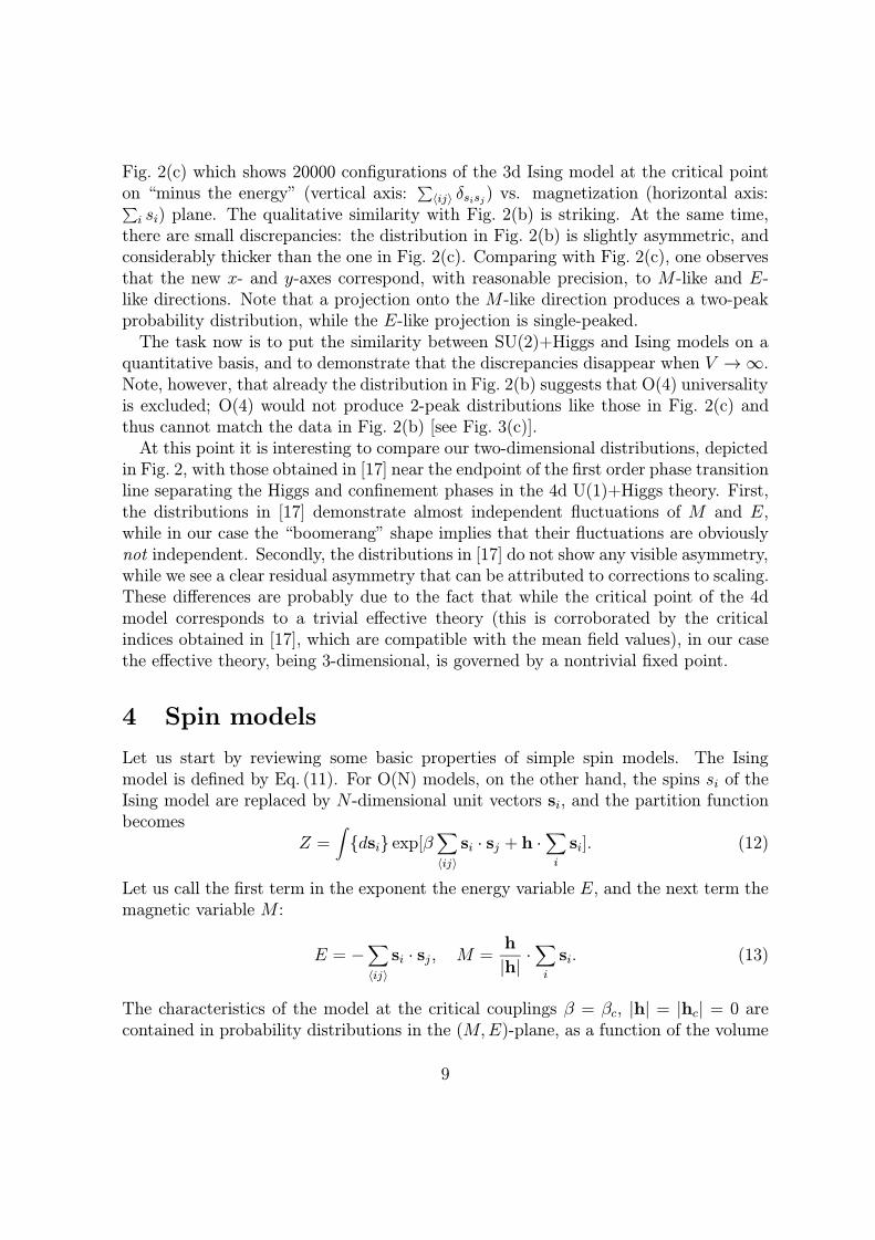
Fig. 2(c) which shows 20000 configurations of the 3d Ising model at the critical pointon “minus the energy” (vertical axis:
∑〈ij〉 δsisj) vs. magnetization (horizontal axis:∑
i si) plane. The qualitative similarity with Fig. 2(b) is striking. At the same time,there are small discrepancies: the distribution in Fig. 2(b) is slightly asymmetric, andconsiderably thicker than the one in Fig. 2(c). Comparing with Fig. 2(c), one observesthat the new x- and y-axes correspond, with reasonable precision, to M-like and E-like directions. Note that a projection onto the M-like direction produces a two-peakprobability distribution, while the E-like projection is single-peaked.
The task now is to put the similarity between SU(2)+Higgs and Ising models on aquantitative basis, and to demonstrate that the discrepancies disappear when V →∞.Note, however, that already the distribution in Fig. 2(b) suggests that O(4) universalityis excluded; O(4) would not produce 2-peak distributions like those in Fig. 2(c) andthus cannot match the data in Fig. 2(b) [see Fig. 3(c)].
At this point it is interesting to compare our two-dimensional distributions, depictedin Fig. 2, with those obtained in [17] near the endpoint of the first order phase transitionline separating the Higgs and confinement phases in the 4d U(1)+Higgs theory. First,the distributions in [17] demonstrate almost independent fluctuations of M and E,while in our case the “boomerang” shape implies that their fluctuations are obviouslynot independent. Secondly, the distributions in [17] do not show any visible asymmetry,while we see a clear residual asymmetry that can be attributed to corrections to scaling.These differences are probably due to the fact that while the critical point of the 4dmodel corresponds to a trivial effective theory (this is corroborated by the criticalindices obtained in [17], which are compatible with the mean field values), in our casethe effective theory, being 3-dimensional, is governed by a nontrivial fixed point.
4 Spin models
Let us start by reviewing some basic properties of simple spin models. The Isingmodel is defined by Eq. (11). For O(N) models, on the other hand, the spins si of theIsing model are replaced by N-dimensional unit vectors si, and the partition functionbecomes
Z =∫{dsi} exp[β
∑〈ij〉
si · sj + h ·∑i
si]. (12)
Let us call the first term in the exponent the energy variable E, and the next term themagnetic variable M :
E = −∑〈ij〉
si · sj , M =h
|h|·∑i
si. (13)
The characteristics of the model at the critical couplings β = βc, |h| = |hc| = 0 arecontained in probability distributions in the (M,E)-plane, as a function of the volume
9

of the system. When the variances of the distributions are normalized to unity, thedistributions have a universal form in the large volume limit; the results for the Ising,O(2) and O(4) models are shown in Fig. 3. To reduce statistical noise, these contourplots, as well as the contour plots in the following pictures, have been smoothed by3×3 matrix averaging. That is, before plotting, the occupation number in every bin isreplaced by the average over 9 bins forming a square around it. The bin size has beenchosen sufficiently small so that smoothing does not induce any significant broadeningof the peaks.
To quantify the characteristics of the probability distributions, one can computedifferent moments. Let ∆E ≡ E − 〈E〉, ∆M ≡ M − 〈M〉. Then the moments ofinterest are:
1. Second moments (specific heat, magnetic susceptibility):
χE = 〈(∆E)2〉/L3, (14)
χM = 〈(∆M)2〉/L3, (15)
where L3 is the volume of the system. The behaviour of these moments as a functionof L is characterized by critical exponents:
χE ∝ Lα/ν , χM ∝ Lγ/ν . (16)
The known results for the exponents appearing here are [25, 14, 26, 27, 28]:
model γ α ν γ/ν α/ν
Ising 1.24 0.11 0.63 1.96 0.17O(2) 1.32 -0.01 0.67 1.96 -0.015O(4) 1.47 -0.25 0.75 1.96 -0.33
The exponent ν is the correlation length critical exponent.2. Higher moments. These characterize for instance the symmetry features of the
probability distributions. In particular, all spin models have, for n = 1, 2, . . .,
〈(∆M)2n+1〉 = 0. (17)
As examples of non-zero values, let us mention that for the 3d Ising model in a largecubic box with periodic boundary conditions, the value of the following ratio is knownwith high precision [29]:
〈(∆M)4〉
〈(∆M)2〉2= 1.604(1). (18)
The asymmetry of the energy distribution of the same system is characterized by
〈(∆E)3〉
〈(∆E)2〉3/2≈ −0.36 (19)
10

(a) (b)
(c)
Figure 3: The smoothed and normalized probability distributions, at the critical point,for (a) the Ising model at the volume 583, (b) the O(2) spin model at 643, (c) theO(4) spin model at 643. The x-axis is the magnetic direction and the y-axis the energydirection.
11

lattice measurements163 200000243 200000323 300000403 350000483 400000643 400000
Table 1: The set of simulations for βG = 5. All simulations have been performed atx = 0.112706, βH = 0.362835, and later reweighted to the estimated position of theinfinite volume critical point: x = 0.11331593, βH = 0.36288657.
(this value corresponds to the simple cubic Ising model on a 583 lattice, where devi-ations from scaling due, in particular, to the presence of a large regular part in theenergy, are still non-negligible).
These ratios, as well as the critical exponents, are universal quantities which canbe used to quantify the similarity or dissimilarity of the endpoint of the SU(2)+Higgstheory with different spin models.
5 Detailed study of the critical region
As discussed above, our computational strategy is based on collecting joint probabilitydistributions of several observables (initially two, as in Fig. 2, and then up to six,as discussed below) for the system in Eq. (4) in a cubic box with periodic boundaryconditions. These are used to
1. find the position of the critical point,2. determine the M-like and E-like directions in the space of observables,3. perform finite size scaling (FSS) to compute critical indices, by studying how the
fluctuations of M-like and E-like observables at the critical point depend on the systemsize,
4. determine higher moments, such as the skewness of E.
Our analysis is based on simulations at βG = 5 with the lattice sizes and statisticsshown in Table 1. In each case the measurements are separated by 4 overrelaxationsweeps and one heat bath/Metropolis sweep. The update algorithms used are describedin Ref. [10]. The relatively coarse lattice spacing was chosen in order to allow for largerphysical volumes, and thus reduce the corrections to scaling at any given lattice size.
12

5.1 Locating the critical point
Let us first recall how one locates the critical point in the case of a one-dimensional,rather than a two-dimensional, parameter space, such as in the case of the spin modelsin Eq. (12). Here the critical point is known to occur at h = 0, and the only parameterwhich remains to be found is βc.
In this case the procedure commonly used is the “intersection of Binder cumulants”[30]. It is based on the following general idea. Consider the system in a finite box ofgiven geometry (say, cubic) with given boundary conditions (say, periodic). Considerany observable (for example, magnetization), averaged over the system. Make a Boltz-mann ensemble of configurations, for each configuration measure this observable andthus construct its probability distribution. Then, if the system is exactly at the criticalpoint and scaling is valid, the form of this probability distribution should be indepen-dent of the system size; only its scale will be changing. Thus any characteristics such asthose in Eqs. (18), (19), designed to be sensitive to the form of probability distributionbut not to the rescaling of the observable, will behave in the following typical way:when plotted as a function of a parameter (for spin systems, as a function of β) forseveral lattice sizes, all plots intersect at the value of the parameter that correspondsto the critical point. This provides a convenient way to locate it.
This approach can easily be generalized to the case of a two-dimensional parameterspace. The main idea remains the same: the critical point is a point where the form oftwo-dimensional distributions, such as those in Fig. 2, does not depend on the systemsize, up to a possibly nonorthogonal linear transformation. To locate the critical point,one now needs two characteristics. For example, if one has somehow found the M-likedirection, one can consider 〈(∆M)4〉/〈(∆M)2〉2 and 〈(∆M)3〉/〈(∆M)2〉3/2. The formeris sensitive to a deviation from the critical point along the (continuation of) the firstorder transition line, while the latter is sensitive to a deviation across the line. Findingthe intersection of these cumulants for two lattice sizes now implies solving a systemof two equations for two variables.
The procedure just described is completely general (however, it remains to be un-derstood how to find the M-like direction; see Sec. 5.2) and does not depend on anyconjecture about the universality class of the critical point. However, it appeared notto be very practical, the main stumbling block being its sensitivity to corrections toscaling, which are in our case non-negligible, as demonstrated by Fig. 2.
A modification of this approach which is more stable against deviations from scaling,relies on a conjecture about the universality class of the critical point. Indeed, if weexpect the critical point to belong to the 3d Ising universality class, we know that inthe scaling limit 〈(∆M)4〉/〈(∆M)2〉2 = 1.604(1) [29], 〈(∆M)3〉/〈(∆M)2〉3/2 = 0. Bysolving these equations, one can find the apparent location of the critical point for eachlattice size separately. The consistency of the conjecture about the universality classcan be checked later: the lattice size dependence of the position of the apparent critical
13

0.0000 0.0001 0.0002 0.00031/volume = 1/L
3
0.106
0.108
0.110
0.112
0.114
xc
βG = 5 critical x
L−3
L−2.4
Figure 4: The reweighted xc from simulations at βG = 5, x = 0.112706, as a functionof the volume.
point should follow the known correction to scaling behaviour.As a variant, one can use the whole probability distribution P (M), which is known
quite precisely for the 3d Ising model, rather than its moments, and require that theapparent critical point for the given lattice size be a point where P (M) matches mostfavourably the Ising P (M), say, by the χ2 criterion. This method has been used in [18]for locating the liquid-gas critical point.
The method we chose to use in practice is as follows. Assume that we have deter-mined an M-like direction, as explained in the next Section. To compute the positionof the apparent critical point for a given lattice size we have reweighted the data for thecorresponding lattice (Table 1) to a trial value of (x, βH) which translates to (βH , βR)according to Eq. (6), computed the probability distribution of the M-like observableP (M) and tuned (x, βH) so that
1. the two peaks of P (M) are of equal weight,2. the ratio of the peak value of P (M) (the average height of the two peaks) to
P (M) at the minimum between the peaks equals the corresponding ratio for the 3dIsing model at the critical point [31]:
Pmax/Pmin = 2.173(4). (20)
The criterion based on the ratio Pmax/Pmin appeared to be less sensitive to asymmetriccorrections, which are most pronounced at the tails of P (M), than the usual one basedon the fourth order cumulant in Eq. (18).
14

The resulting dependence of the apparent position of the critical point on the latticesize is shown in Fig. 4. It follows nicely the law based on Ising-type corrections toscaling, the deviation of xc from the limiting value behaving as
xc(L)− xc(∞) ∝ L−(∆+1)/ν ≈ L−2.4, (21)
where ∆ = 0.52(4) is the universal correction to scaling exponent for the 3d Isinguniversality class. Thus the determination of the critical point based on the expectedIsing-like properties is completely consistent. However, the statistical errors of thedatapoints are large enough so that a regular L−3 -behaviour cannot be ruled out,either. Nevertheless, the variation of the infinite volume critical point is quite small, andit has a negligible effect on the analysis below. The infinite volume result, determinedby the L−2.4-fit, is xc(∞) = 0.1133(25). In the following analysis we always reweightthe data to the critical point xc = 0.11331593, βH = 0.36288657. Due to the strongcorrelations in coupling constants both have to be fixed to a high numerical precision.
5.2 Determining M-like and E-like observables
We observed that even the problem of locating the critical point, to say nothing offurther quantitative analysis, depends on finding the M-like direction in the space ofobservables. In Fig. 2, this is done by letting the M-like direction go along the prob-ability distribution, and taking the E-like to be orthogonal to it. The result appearsto be very encouraging, by the eye, when compared with the 3d Ising distribution inFig. 2(c). This approach relies on the fact that the distribution is extremely elongated,and becomes even more so with growing lattice size, fluctuations of M growing muchfaster than those of E: 〈(∆M)2〉/〈(∆E)2〉 ∝ L(γ−α)/ν ≈ L1.8.
The determination of the M-like and E-like directions can now be put on a quan-titative basis as follows. Take the probability distribution P (Shopping, S(φ2−1)2). Com-pute the fluctuation matrix and find its eigenvectors. The larger eigenvalue will give〈(∆M)2〉, the smaller one 〈(∆E)2〉, while the corresponding eigenvectors will give theM-like and E-like directions.
The procedure just described is identical to the one used in [17] and completelyignores the possibility that the M-like and E-like directions can be nonorthogonal inthe original basis chosen [24, 18]. However we have found that both this simplisticprocedure and its generalization to a larger space of observables, which is discussedbelow, work extremely well for our system, while the more sophisticated approach of[18] runs into serious difficulties. This seems to be an interesting point that deservessome discussion, as it probably means that asymmetric corrections to scaling play amore prominent role in our system than in the liquid-gas models (see also Sec. 6).
The method of [18] employs the matching of the probability distribution of a linearcombination of the two basic observables to P (M) known from the 3d Ising model atcriticality, to find the M-like direction simultaneously with the apparent critical point
15

(performing a search in 3-dimensional space: two parameters for a trial critical point,plus one parameter for a trial M-like direction). After that, the E-like direction isfound by matching the distribution of a trial linear combination of observables to the3d Ising P (E).
One of the key statements of [18] is that the pronounced asymmetry of two-peakprobability distributions of various observables at the critical point can be attributedto the fact that they are actually mixtures of M and E, while the distribution of Mitself comes out completely symmetric, within the accuracy of the simulation. Onecan, however, raise the following question: is it not possible that the perfect symmetryof P (M) emerges as an artefact of the procedure (optimization of its matching to theexactly symmetric P (M)Ising)?
This problem can be also put as follows. We have the two-dimensional probabilitydistribution for our system, as in Fig. 2(b), now as a function of four parameters: thetrial critical point and two trial directions for M and E (not necessarily orthogonal).On the other hand, we have the corresponding P (M,E)Ising for the Ising model atcriticality, Fig. 2(c), with its projections P (M)Ising and P (E)Ising. The question is, isit a good idea to look for the M-like and E-like directions by requiring that just theone-dimensional projections of Figs. 2(b) and 2(c) onto the horizontal and vertical axesmatch each other? Should not one rather match the whole distributions?
Obviously, in the absence of deviations from scaling it would make little differencewhether to match the whole distributions or their one-dimensional projections: bothmethods would converge to the same result, corresponding to a perfect matching. Theproblem, however, becomes nontrivial when there are deviations from scaling, especiallythe asymmetric ones. Concretely, we have found that for our system, an application ofthe procedure in [18] appeared to be completely misleading.
The observation is that for practically achievable lattices, there is a significant asym-metry in two-dimensional distributions, as seen in Fig. 2(b). This asymmetry appearsto be unremovable (more precisely, only a relatively small part of it can be removed)by any choice of (nonorthogonal) directions for M and E. This can be understoodwhen one notices that one of the characteristic features of this asymmetry is the dif-ference of areas under the two peaks of the probability distribution (see also Figs. 5),which cannot be cured by any linear transformation, even nonorthogonal, as such atransformation keeps the ratio of areas invariant.
Thus if we try to symmetrize the two-dimensional distribution (or match it to theIsing form Fig. 2(c)), a considerable asymmetry remains and, notably, P (M) comesout considerably asymmetric (Fig. 5, right). At the same time, matching P (M) toP (M)Ising easily finds the “M-like” direction that ensures a perfect matching andthus symmetric P (M) (Fig. 6). But this optimization of the symmetry of the one-dimensional projection is achieved at the price of greatly reducing, rather than improv-ing, the symmetry of the two-dimensional histogram as a whole and thus should beconsidered completely misleading!
16

(a) 0
0.1
0.2
0.3
0.4
0.5
0.6
-2 -1 0 1 2
16**3Fit
Ising at T_c
(b) 0
0.1
0.2
0.3
0.4
0.5
0.6
-2 -1 0 1 2
32**3Fit
Ising at T_c
(c) 0
0.1
0.2
0.3
0.4
0.5
0.6
-2 -1 0 1 2
64**3Fit
Ising at T_c
Figure 5: The probability distributions P (M,E) (left) and P (M) (right) at the infinitevolume critical point, for the volumes (a) 163, (b) 323, (c) 643. It is seen how thedistribution becomes more symmetric for increasing volumes. The M and E directionshave been found with a 6-dimensional fluctuation matrix analysis, see Sec. 5.2.1.
17

0
0.1
0.2
0.3
0.4
0.5
0.6
-2 -1 0 1 2
16**3: M with admixture of EIsing at T_c
Figure 6: This figure shows that it is possible to find a direction for M that provides aperfectly symmetric P (M), but only at the price of reducing the symmetry of P (M,E).The data are the same as in Fig. 5(a).
Thus we have found the following important differences between our system and theliquid-vapour models [18]:
1. Our system demonstrates non-negligible asymmetric corrections to scaling. Theseshow up in two-dimensional distributions and cannot be removed by any choice of Mand E. As a consequence, asymmetries of various one-dimensional distributions aremostly caused by them, and not so much by the admixture of E, as in [18].
2. In our system, we do not find much evidence of the possible nonorthogonality ofthe M-like and E-like directions. Deviations from orthogonality, if any, can be safelyneglected, in clear distinction from [18] where they played quite a prominent role.
In conclusion, after having tried four methods for determining the M-like and E-likedirections,
(a) finding the eigenvectors of the fluctuation matrix [17],(b) matching P (M) to P (M)Ising, P (E) to P (E)Ising [18],(c) matching P (M,E) to P (M,E)Ising,(d) maximizing the symmetry of P (M,E),
we arrived at the conclusion that the method (a) works best for our system, method(b) appears to be misleading, and methods (c) and (d) produce results consistent with(a), while being much more difficult to implement and use. One of the tricky pointsis the multidimensional minimization of the difference of two Monte Carlo generatedtwo-dimensional probability distributions, which is typically a very noisy function (theproblem is alleviated by first smoothing the histograms, then minimizing their dif-ference). Another stumbling block of the method (c) is that a seemingly harmlessmanifestation of deviations from scaling — the excessive thickness of P (M,E) com-
18

Figure 7: The dependence of the probability distribution P (M,E) on the number ofobservables, for a βG = 5, 643 lattice. Left: The diagonalized fluctuation matrix fortwo observables Shopping, S(φ2−1)2 , see Eq. (4). Right: The same for four observables,SG, Shopping, Sφ2, S(φ2−1)2 . It is seen that the distribution becomes sharper, or thinner,as the basis is expanded. Using six observables leads to a still sharper distribution, seeFig. 5(c).
pared with P (M,E)Ising — has a very strong effect on their difference, in terms of χ2,making it impossible to achieve a good matching.
5.2.1 Extending the space of observables
The main observation so far was that while the form of the probability distributionat the critical point comes out strikingly similar to that of the 3d Ising model, asdemonstrated by Figs. 2(b,c), there are still differences (asymmetry and thickness) thatare decreasing with growing lattice size, but relatively slowly, so that, for example, theelimination of the thickness would require prohibitively large lattice sizes.
The situation can be considerably improved by further generalizing the procedureof determining the M-like and E-like observables. The reasoning behind this is asfollows. If we consider any arbitrary observable (say, Shopping), it behaves at the criticalpoint more or less like magnetization, and its probability distribution also looks verysimilar to the distribution of magnetization, the main feature being the double-peakstructure. However, it shows a certain asymmetry, which eventually goes down to zerowith growing lattice size. This can be understood as a consequence of the fact that weexpect any observable to behave at the critical point as a sum of M-like, E-like andregular contributions. Their dependence on the lattice size is different and is governed,correspondingly, by Lγ/ν , Lα/ν and L0. On large lattices the magnetic contribution isalways dominating, so any given observable starts behaving as the M-like.
19

Figure 8: The joint probability distribution of observables corresponding to the largest(horizontal axis) and second largest (vertical axis) eigenvalues of the 4× 4 fluctuationmatrix of the terms in Eq. (4).
From this point of view, when we study the joint distribution of two observables andfind the M-like and E-like directions as the primary axes of the corresponding veryelongated fluctuation ellipse, we are actually finding the E-like direction as a linearcombination of observables in which the dominating M-like terms cancel each other.Thus the consideration of two-dimensional distributions provides a way to disentanglethe dominant (M-like) and subdominant terms. However, it becomes clear that withinthis approach the E-like observable will collect all subdominant terms, both actuallyE-like and regular.
Thus one arrives at the idea that a further separation of E-like and regular con-tributions could be achieved by generalizing the procedure to more observables thantwo. The hope is to “purify” the E (for M there is little difference, as it outweighseverything else by orders of magnitude anyway).
To begin with, we have considered the 4-dimensional space of observables, these ob-servables being the four terms in the action in Eq. (4). Diagonalizing the 4× 4 matrix〈(Si − 〈Si〉)(Sj − 〈Sj〉)〉 for the 643 lattice (βG = 5) resulted in the eigenvalues and-vectors shown in Table 2. We observe a pronounced hierarchy of eigenvalues, similarto the previously considered case of two observables, Fig. 2(a). The largest eigenvaluecorresponds, as expected, to M . However, E turns out to correspond, somewhat sur-prisingly, to the smallest eigenvalue, rather than to the second largest one, while the twoeigenvalues in the middle correspond to regular directions. This is substantiated bothby analysing the dependence of the eigenvalues on the lattice size and by looking at thejoint probability distributions of various pairs of the 4 observables corresponding to the4 eigenvectors. The joint distribution of projections onto eigenvectors corresponding
20

to the largest and to the smallest eigenvalue is depicted in Fig. 7(right); projectionsonto eigenvectors corresponding to the largest and to the second largest eigenvalue pro-duce a strikingly different pattern, Fig. 8, signalling that the second largest eigenvaluedoes indeed correspond to a regular observable: its fluctuations are Gaussian-like andindependent from those of M .
It is evident in Fig. 7 that the extension of the space of observables from two- tofour-dimensional does indeed considerably reduce the deviation of P (M,E) from the 3dIsing scaling form. The most notable effect is the reduction of the excessive thicknessof P (M,E). Now the question is, what happens if we further extend the space ofobservables, having in mind that if one wants to sort out E as well as possible, onewould like it to correspond to an eigenvalue which is not the smallest one (as thesmallest one is just collecting all unresolved contributions). Thus we have added twoadditional observables: the sum of the absolute values of the Higgs field, and the analogof the hopping term, where the Higgs matrices have been replaced by SU(2) matrices,dividing out the length of the Higgs field:
SR ≡∑x
R(x), SL ≡∑x,i
1
2TrV †(x)Ui(x)V (x + i), (22)
where Φ(x) = R(x)V (x), R ≥ 0, V ∈ SU(2).Now the energy eigenvalue appears to be the fourth of six, in descending order, and we
observe further significant reduction of difference between P (M,E) and P (M,E)Ising,as seen in Fig. 5(c).
One could continue extending the space of observables (in principle, there are in-finitely many gauge invariant operators to be considered), but these six operators seemto be enough for our purposes.
The coefficients of the different eigenvectors in terms of the original operators inEqs. (4),(22), together with the eigenvalues, are shown in Table 2. We observe thefollowing:
1. While the eigenvectors corresponding to the three largest eigenvalues are relativelystable with respect to an increase in the number of basis vectors, the E directionchanges considerably. However, the final critical distributions, critical indices, etc, arequite stable.
2. The largest eigenvalue, the magnetic one, is about 4 orders of magnitude largerthan the next largest, for the volumes used.
3. The second largest eigenvalue consists almost solely of the plaquette term of theaction, and conversely, the plaquette term contributes significantly only to the secondeigenvalue. Thus, the plaquette term is practically decoupled from the other modes.
4. At very large volumes the energy eigenvalue will overtake the two regular eigen-values above it and become the second largest one (Sec. 5.3). However, for the rangeof volumes studied here, the hierarchy shown in Table 2 was preserved.
21

direction λ c1 c2 c3 c4 c5 c6
4 operatorsM 1.28×10¹⁰ 0.05142 0.72590 -0.68564 -0.01808 – –regular 8.51×10⁵ 0.9965 0.008 0.083 0.0049 – –regular 2.59×10⁵ -0.066 0.6877 0.7227 0.0185 – –E 1.75×10³ -0.0027 0.0004 -0.0262 0.99965 – –
6 operatorsM 1.33×10¹⁰ 0.0505 0.7133 -0.67375 -0.01777 -0.1646 -0.0853regular 8.52×10⁵ 0.9954 0.010 0.087 0.0055 0.0082 -0.037regular 2.81×10⁵ -0.078 0.655 0.6876 0.0262 0.136 -0.271E 1.32×10⁵ 0.024 0.233 0.033 -0.1052 0.450 0.855regular 4.05×10³ 1×10⁻⁵ -0.0914 -0.241 -0.217 0.836 -0.433regular 73 -2×10⁻⁵ 9×10⁻⁵ -0.0816 0.9700 0.229 0.0019
Table 2: The eigenvalues λ and the coefficients ci for the diagonalized directions, interms of the operators in Eqs. (4),(22). Here the volume is 643, βG = 5, and the datahave been reweighted to the infinite volume critical point.
5.3 Critical indices
Now that the M- and E-like directions have been determined, one can find the crit-ical indices, using the finite size scaling formulas in Eq. (16). The scaling has to bestudied at the infinite volume critical point xc(∞), whose determination was discussedin Sec. 5.1. There is a small dependence of eigenvectors on the lattice size, due tocorrections to scaling; we take a fixed set of eigenvectors (corresponding to the largestlattice, 643) and compute the second moments of the corresponding projections, for aset of lattice sizes. The dispersion of M grows approximately as L4.92, the dispersionof E grows as L3.27, and those of the remaining projections grow as L3, as shown inFigs. 9, 10. (An additional volume factor enters due to observables being sums over thelattice, without dividing by the volume). The apparent value of α/ν ≈ 0.27 deviatesnotably from the Ising asymptotic value 0.17, but just the same effect is observed forthe Ising model itself, for similar lattice sizes. This is explained by the presence of anegative regular background in χE [13], as shown in Fig. 9.
In addition to the critical exponents γ/ν and α/ν, which are related to the secondmoments of the distributions P (M) and P (E), we have also determined the correlationlength critical exponent ν. In models with an exact symmetry M ↔ −M (like the Isingmodel), finite observables like the Binder cumulant
UL ≡ 1−1
3
〈M4〉
〈M2〉2(23)
can be assumed, near the critical point, to be regular functions of ξ/L, the ratio of the
22

10 20 40 70 100L
0.95
1.00
1.05
1.10
1.15
χ M/χ
Isin
g
βG = 5 magnetic exponent
L1.92−1.96
10 20 40 70 100L
0.3
0.4
0.5
0.6
χE
βG = 5 energy exponent
0.16 L0.27
−0.23 + 0.36 L0.17
L0.17 Is
ing (asymptotic)
Ising
(actu
al)
Figure 9: Left: the magnetic susceptibility χM divided by the Ising scaling law const×L1.96. The corresponding critical exponent is γ/ν = 1.92(3), whereas Ising model hasγ/ν = 2− η ≈ 1.96. It is seen that at larger volumes the results for χM are consistentwith the Ising model. The absolute value of χM is ∼ 5 × 10⁴ at L = 64. Right:the energy susceptibility χE. Note that the absolute value is much smaller than forχM . Two different fits to the datapoints are shown. It is seen that the behaviour isconsistent with that of the Ising model (which is described by χE = −11.1 + 14.6L0.17
[13] and is shown here up to an arbitrary overall factor, so only its slope is relevant).O(N) models with N ≥ 2 have a negative exponent for χE and are thus excluded.
correlation length to the system size. As ξ ∼ t−ν , the exponent ν can be obtained fromthe slope of UL at the critical point [30]:
∂UL∂t∝ L1/ν . (24)
The SU(2)+Higgs theory lacks the explicit M ↔ −M -symmetry, and we use the M-and E-like eigenvectors in the analysis. Furthermore, we substitute M → ∆M =M − 〈M〉 in the Binder cumulant. Let us now denote by βE the coupling constant ofthe E-like eigenvector: that is, we formally extend the lattice action in Eq. (4) to theform S + βEE, where βE = 0 at the critical point. We then obtain from Eqs. (23) and(24) that
∂UL∂βE
= (1− UL)
[〈E〉+
〈(∆M)4E〉
〈(∆M)4〉− 2〈(∆M)2E〉
〈(∆M)2〉
]. (25)
This expression is readily evaluated using the M- and E-like eigenvectors at the criticalpoint. The results are shown in Fig. 11. With these volumes the corrections to scalingare still substantial, and the points do not fall on a straight line on a log-log plot.
23

10 20 40 70 100L
0.950
0.975
1.000
1.025
1.050
1.075
χi
βG = 5 non−diverging modes
λ1 = 3.244(4)λ2 = 1.071(2)λ3 = 0.01552(2)λ4 = 2.79(1) x 10
−4
Figure 10: The regular eigenvalues, divided by the volume, as a function of the latticesize. The normalization is arbitrarily chosen such that the average of the values shown is1.0; the absolute values are as indicated by the numbers. It is seen that the eigenvaluesare constant with a very good accuracy (note the scale of the y-axis). The smallesteigenvalue has the largest volume dependence as it is contaminated by higher states.
Taking into account the corrections to scaling, we fit the data with the 4-parameteransatz
∂UL
∂βE= c1 L
1/ν(1− c2 L
−ω). (26)
However, with only 6 points and relatively large statistical errors (when compared with,say, the Ising model simulations [28]) the error range in the correlation length criticalexponent becomes rather large: the result is ν = 0.63(17). If we lock the correction toscaling exponent ω to the central value ω = 1.7 and perform a three-parameter fit, theresult becomes ν = 0.63(3).
The value of ν is completely compatible with the Ising model (but also with O(2)).However, in the Ising model the correction to scaling exponent is ω = 0.8, whichdoes not fit the data well. This is very likely due to the asymmetry in the P (M,E)-distributions of the smallest volumes (Fig. 5). In order to observe the Ising-type correc-tions to scaling one should use volumes which are large enough so that the asymmetriccorrections to scaling have become subdominant. This is discussed in more detail inthe next section.
Apart from the second moments χE, χM , we have also measured the third moment ofE and the corresponding skewness ratio in Eq. (19). The results are shown in Fig. 12.
24

10 20 40 70 100L
1
10
100
dU
L/d
β E
βG = 5 correlation length exponent
c1L1/ν
(1 + c2L−ω
)
Figure 11: The slope of the Binder cumulant UL at the critical point in the E-likedirection versus the lattice size. The dashed line is a 4-parameter fit to the data.
They are consistent with those of the Ising model, but differ from O(2) and especiallyfrom O(4), in which case the skewness of P (E) is very small.
6 Dependence of asymmetry on the volume
Significant asymmetry effects were observed in the previous analysis of the SU(2)+Higgs theory. Here we study them in some more detail. We consider the distribu-tions P (M) at the critical point, as shown in Fig. 5(right), and attempt to obtain aquantitative description of how they approach the Ising shape with growing lattice size.
It is well-known [32] that the leading corrections to scaling in an exactly symmetricsystem, such as the Ising model itself, show the universal behaviour governed by L−ω,ω ≡ ∆/ν ≈ 0.8 (see also Sec. 5.1). However, the asymmetric corrections, which arealso present in our system, have their own critical exponent ω5, which is different fromω and has attracted much less attention in the literature (to our knowledge, it hasnever been studied before in the framework of Monte Carlo simulations). Including theoperators φ5, φ6 in Eq. (10), the exponent ω5 has been computed within the ε-expansionup to order ε3 [33]–[35], and within the renormalization group framework [36]. Quotingfrom [35],
ω5 = 1 +11
6ε−
685
324ε2 +
107855 + 103680ζ(3)
34992ε3 +O(ε4). (27)
25

0.00 0.02 0.04 0.06 0.081/L
−1.5
−1.0
−0.5
0.0
0.5
<(E
−<E
>)3 >
/<(E
−<E
>)2 >
3/2
Skewness of energy distributions
SU(2)−Higgs
Ising
O(2)
O(4)
Figure 12: The skewness of P (E) for 3d SU(2)+Higgs and different spin models, versusthe inverse lattice size.
This series behaves poorly at ε = 1, resulting in 1 + 1.83− 2.11 + 6.64 . . .. An attemptto improve the situation using Pade approximants produces the sequence 2.83, 1.85,2.32, in orders O(ε), O(ε2), O(ε3) respectively, leading to the estimate that ω5>∼ 1.5[35]. This estimate has been confirmed by the computation within the renormalizationgroup [36], which resulted in ω5 = 2.4(5). Thus it is generally believed (see, e.g.,[37]), that ω5 ≈ 2.1 (the average of the last two Pade values). This implies that theasymmetric corrections, going as L−ω5, should die out very rapidly when a criticalpoint is approached, not only faster than the leading symmetric corrections (L−ω), butalso faster than the subleading ones (L−2ω), and thus be of no practical importanceanywhere near the critical point. This is probably the reason why ω5 is rarely discussedin the literature.
However, we do observe significant asymmetric contributions, and it is interesting tosee what kind of implications there are for ω5. For this purpose we need to quantify thedeviation of P (M) from the Ising scaling form (Fig. 5, right). As has been found in [31],the scaling form of P (M) for the 3d Ising model in a cubic box with periodic boundaryconditions is described extremely well by the following simple approximation:
P (M) ∝ exp{−(M2
M20
− 1)2(
aM2
M20
+ c
)}, (28)
where M0 is the position of the magnetization peak, and the universal constants a and
26

c are
a = 0.158(2), (29)
c = 0.776(2).
The generalization of Eq. (28) for our case must also include odd powers of M , and canbe written down as follows:
P (M) ∝ e−Veff , Veff = (x2 − 1)2(ax2 + bx+ c)− hx, x =M −M1
M0. (30)
This Veff can be considered as a special parametrization of a general double-well polyno-mial of up to sixth order in M . The parameters M0 and M1 are responsible for rescalingand shifting the distribution as a whole. Two of the remaining four parameters, b andh, characterize the asymmetry of P (M).
One of them, h, is sensitive to what may be called the superficial asymmetry: anasymmetry caused by a small deviation of parameters of our system from the truecritical point across the first order line, which is, in the case of the Ising model, equiv-alent to an application of a small external field. This parameter is also sensitive to theasymmetry caused by statistical errors in the relative heights of the two peaks, whichemerge on larger lattices as a consequence of the growth of the tunnelling time withthe lattice size.
On the other hand, the parameter b characterizes what may be called the genuineasymmetry, and is responsible for the difference in the peak widths that remains afterwe make them equally high by slightly shifting the system across the phase transitionline (that is, in the h-like direction).
Thus we will be interested in three parameters: a, b and c. Making a 6-parameterfit to our data, we observe (Fig. 5, right) that the ansatz in Eq. (30) is indeed able toprovide a sufficiently good approximation. The quality of the approximation turns outnot to be exactly as excellent as in the case of the 3d Ising model (one observes, forexample, that the fit tends to go a little bit above the top of the higher peak), butquite sufficient for our purposes.
The results for a, b and c are shown in Fig. 13. One observes that all three parametersgo in the directions of the corresponding Ising limits, with growing lattice size.
The parameter c falls reasonably well on a straight line which corresponds to thestandard correction to the scaling exponent ω ≈ 0.8. It is interesting to note thatit approaches the scaling limit from below, while in the simple cubic Ising model itapproaches the same limit from above [31].
The parameter a behaves less nicely but is also consistent with ω ≈ 0.8 for largerlattice sizes. As for the parameter b, which is expected to behave as L−ω5 , it doesindeed decrease with growing lattice size, but much more slowly than implied by thegenerally accepted high value of ω5. In fact, b seems to go down more slowly thanL−0.8, rather than going as L−2.1 (the data in Fig. 13 are best fitted by L−0.4 . . . L−0.5)!
27

0.00 0.02 0.04 0.06 0.08 0.10 0.12L
−0.8
0.0
0.2
0.4
0.6
0.8
1.0
a,
b,
c
abc
Isin
g m
odel
val
ues
Figure 13: The parameters a, b, c that determine the shape of P (M) according toEq. (30), as a function of the lattice size (L = 16 . . . 64). The values in Eq. (29) for theIsing model in the scaling limit are marked on the left edge of the plot.
The origin of this contradiction remains unclear. It might be that our lattices arestill too small, and we have not yet reached the asymptotic regime where asymmetriccorrections behave as L−ω5 . On the other hand, something might be missing in thetheoretical treatment of asymmetric corrections to scaling. This question certainlydeserves further study.
7 Summary of the results
The aim of this paper was to study the universality properties of the endpoint of theline of first order phase transitions in the 3d SU(2)+Higgs gauge theory. Qualitatively,the result was obvious when comparing the two-dimensional near-endpoint distributionof this theory in E- and M-like variables, shown in Fig. 2(b), with the correspondingdistribution for the 3d Ising model shown in Fig. 2(c): the distributions look extremelysimilar. The bulk of this paper was devoted to putting this similarity on a strictquantitative basis.
Indeed, the two main discrepancies between Figs. 2(b) and 2(c) – the asymmetryand the thickness of Fig. 2(b) – can be removed by going to the infinite volume limitand by using a larger basis of observables. The effect of the volume variations is shownin Fig. 5. It is seen that as the volume is increased, the distribution looks more andmore like that of the Ising model, Fig. 3(a). The effect of the choice of basis is shown in
28

Fig. 7. It is seen that the thickness is removed as one goes from two to four observables,and even more as one goes to six observables (Fig. 5(c)). The fact the Fig. 5(c) agreeswith Fig. 3(a) and not with Figs. 3(b),(c), is our main result.
Furthermore, the basis of six observables allows to construct a 6 × 6 correlationmatrix, which is then diagonalized. It turns out that two of the eigenvalues showcritical behaviour, whereas four are regular. The largest eigenvalue corresponds toχM . The susceptibilities χM , χE are shown in Fig. 9 as a function of the volume. Thebehaviour is clearly consistent with that of the Ising model. For the energy exponentχE even the fact that scaling violations are large at moderate volumes is reproduced.An O(4) model with a negative exponent for χE is excluded.
The remaining four regular exponents are shown in Fig. 10. They show no criticalbehaviour as a function of the volume.
Apart from the second moments χE, χM , we have measured the correlation lengthcritical exponent ν (Fig. 11) and the skewness of P (E) (Fig. 12). The results arecompletely consistent with those of the Ising model.
Based on the values of the critical exponents and properties of P (M,E), P (M)and P (E), we thus conclude that the endpoint of the SU(2)+Higgs theory is in theuniversality class of the 3d Ising model.
We have also studied corrections to scaling. While “symmetric” corrections to scalingdisplay precisely the exponent inherent for the 3d Ising model (Sec. 5.1), asymmetriccorrections to scaling, which arise from higher order operators not appearing in the ac-tions in Eqs. (10), (11), behave in an unexpected way: they are quite large at reasonablelattice sizes.
7.1 The continuum limit of xc
Finally, let us discuss the continuum limit of xc, the location of the endpoint, whichis a non-universal quantity. This requires measurements performed at different latticespacings; for βG = 8 we used a set of simulations originally described in [1], and forβG = 12 we used the critical coupling measured in [3]. The results are shown in Fig. 14.The improved values for xc have been obtained from Eq. (9). As the corrections linearin 1/βG are thus removed, a quadratic extrapolation can be made. The continuumresult is
xc = 0.0983(15). (31)
We estimate that the effect of the U(1) group on xc is <∼ 10%. According to theformulas in [7], the value of xc in Eq. (31) corresponds to mH = 72(2) GeV in theSM, and xc = 0.11 would correspond to mH = 77(2) GeV. In the MSSM, the sameeffective theory as in Eq. (1) can be derived, just the relations to 4d parameters aredifferent [19]. Then the value x = xc can correspond to many different Higgs masses,depending on the other parameters of the theory: some examples are shown in Fig. 15.
29

0.00 0.05 0.10 0.15 0.201/βG
0.09
0.10
0.11
0.12
xc
Critical x
βG = 5,8βG = 12,16 [Guertler et al.]βG = 5,8 improvedβG = 12,16 improved [Guertler et al.]
Figure 14: The infinite volume extrapolations of xc as a function of βG. Gurtler et alrefers to [3]. The location of the endpoint has been determined in [2], as well, but thevolumes there were somewhat smaller so that the inclusion of that datapoint is notmeaningful. The improved values have been obtained from Eq. (9).
8 Conclusions
In this paper, we have shown that the endpoint of the line of first order transitionsin the 3d SU(2)+Higgs theory is a second order transition in the universality class ofthe 3d Ising model. In particular, the measured critical exponents, cumulant ratios,and probability distributions of these two theories approach each other with growinglattice size.
To arrive at this conclusion, we have developed a general method to determine theuniversality class of a phase transition in a completely non-perturbative system, utiliz-ing lattice Monte Carlo simulations. The method can be applied to any system exhibit-ing critical behaviour, provided that it is possible to perform Monte Carlo simulationson the critical point itself. This includes, e.g., the endpoints of the 1st order lines in the3d SU(2)+adjoint Higgs theory (where the line ends [39, 40]), the 3d SU(3)+adjointHiggs theory (where the line turns into a second order line after a tricritical point) orin the U(1)+Higgs theory. On the other hand, the two flavour 4d finite temperaturechiral transition in QCD occurs at the limit mq → 0, which is not directly accessiblewith standard Monte Carlo methods.
We have also determined the continuum extrapolation of an important non-universal
30

180.0 200.0 220.0 240.0m~
75.0
80.0
85.0
90.0
95.0
mH
x=0.0983
tR
mA=300 GeV
mA=200 GeV
mA=150 GeV
mA=120 GeV
mtop=175 GeVmQ=mD=300 GeVAt=0 GeV~
Figure 15: Examples of parameter values corresponding to x = xc in the MSSM [38].Here mtR
is the right-handed stop mass, mH is the lightest CP-even Higgs mass andmA is the CP-odd Higgs mass. The squark mixing parameters have been put to zero.
quantity, the location of the endpoint xc. In the Standard Model with sin2 θW = 0,the resulting value xc = 0.0983(15) corresponds to a physical Higgs mass mH = 72(2)GeV. While taking sin2 θW = 0.23 does not change the universal properties, the valueof xc may grow slightly. However, we do not expect values larger than xc = 0.11,corresponding to mH = 77(2) GeV. Even this Higgs mass is already excluded experi-mentally, and thus there is no phase transition in the Standard Model. If low energysupersymmetry is realized, in contrast, the cosmological electroweak phase transitioncan be of the first order for the Higgs masses allowed at present. This could lead toimportant cosmological consequences.
Acknowledgments
We gratefully acknowledge useful discussions with U.M. Heller and T. Neuhaus. Thesimulations were performed with a Cray T3E at the Center for Scientific Computing,Finland. The work of MT was supported by the Russian Foundation for Basic Re-search, Grants 96-02-17230, 16670, 16347, and that of KK by the TMR network FiniteTemperature Phase Transitions in Particle Physics, EU contract no. FMRX-CT97-0122.
31

Appendix
In this appendix we discuss two points concerning the scalar effective theory in Eq. (10):the relative roles of the linear and cubic terms and discretization. The cubic term isoften used to generate a first order transition, but here it proves convenient to shift itaway.
Consider the theory
S =∫d3x
[1
2∂iφ∂iφ+ hφ+
1
2m2φ2 −
1
3δφ3 +
1
4λφ4
]. (32)
Due to superrenormalisability, only the two 2-loop diagrams
are logarithmically divergent and lead to the following renormalisation scale depen-dence of the mass and magnetic field terms in the MS scheme:
h(µ) =2λδ
16π2log
Λh
µ, m2(µ) =
−6λ2
16π2log
Λm
µ. (33)
The theory now is specified by the four constants λ, δ,Λh,Λm or, equivalently, by
λ, x =m2(λ)
λ2, y =
h(λ)
λ5/2, z =
δ
λ3/2. (34)
However, as there is no φ ↔ −φ symmetry, one can perform a shift φ → φ+constantand choose the constant so that the cubic term disappears. This corresponds to theinvariance of the theory under the transformation (x, y, z)→ (x+ zy/3− 2z3/27, y −z2/3, 0). Thus one can from the outset choose δ = 0 in Eq. (32). The magnetic fieldterm is then scale invariant (see Eq. (33)). However, it is not possible to eliminate thelinear term: it is anyway generated by radiative effects according to Eq. (33).
On the lattice the action corresponding to the theory without the cubic term becomes(after scaling aφ2 → βHφ
2)
S = −βH∑x,i
φ(x + i)φ(x) + β1
∑x
φ(x)
+∑x
φ2(x) +β2H
4βG
∑x
[φ2(x)− 1]2, (35)
32

where the lattice couplings βH , βG, β1 are related to λa, x, y by
λa =1
βG,
x = 2β2G
(1
βH− 3−
βH2βG
)+
3Σ
4πβG −
6
16π2log(6βG + ζ), (36)
y =β1√βH
β5/2G .
Here Σ, ζ are the same as in Eq. (7). Eq. (35) is a standard scalar lattice action butwith very specific couplings, determined by Eqs. (36). If the expectation value of φmeasured with Eq. (35) is 〈φL〉, then in continuum normalisation,
〈φ〉/λ1/2 =√βHβG〈φL〉. (37)
If higher order operators are included in Eq. (32), then the cubic term cannot, ingeneral, be shifted away any more. It becomes a running parameter which is generatedradiatively even if shifted away at some scale.
References
[1] K. Kajantie, M. Laine, K. Rummukainen and M. Shaposhnikov, Phys. Rev. Lett.77 (1996) 2887 [hep-ph/9605288].
[2] F. Karsch, T. Neuhaus, A. Patkos and J. Rank, Nucl. Phys. B (Proc. Suppl.) 53(1997) 623 [hep-lat/9608087].
[3] M. Gurtler, E.-M. Ilgenfritz and A. Schiller, Phys. Rev. D 56 (1997) 3888 [hep-lat/9704013]; M. Gurtler, E.-M. Ilgenfritz, A. Schiller and G. Strecha, Nucl. Phys.B (Proc. Suppl.) 63 (1998) 563 [hep-lat/9709020].
[4] W. Buchmuller and O. Philipsen, Nucl. Phys. B 443 (1995) 47 [hep-ph/9411334].
[5] The Aleph Collaboration, ALEPH 98-029, 26 March 1998.
[6] P. Ginsparg, Nucl. Phys. B 170 (1980) 388; T. Appelquist and R. Pisarski, Phys.Rev. D 23 (1981) 2305.
[7] K. Kajantie, M. Laine, K. Rummukainen and M. Shaposhnikov, Nucl. Phys. B458 (1996) 90 [hep-ph/9508379]; Phys. Lett. B, in press [hep-ph/9710538].
[8] K. Jansen, Nucl. Phys. B (Proc. Suppl.) 47 (1996) 196 [hep-lat/9509018].
[9] K. Rummukainen, Nucl. Phys. B (Proc. Suppl.) 53 (1997) 30 [hep-lat/9608079].
33
[10] K. Kajantie, M. Laine, K. Rummukainen and M. Shaposhnikov, Nucl. Phys. B466 (1996) 189 [hep-lat/9510020].
[11] K. Kajantie, M. Laine, K. Rummukainen and M. Shaposhnikov, Nucl. Phys. B493 (1997) 413 [hep-lat/9612006].
[12] For a recent quantitative study of the 3d Ising model, see M. Caselle and M.Hasenbusch, J. Phys. A 30 (1997) 4963 [hep-lat/9701007].
[13] M. Hasenbusch and K. Pinn, HUB-EP-97/29 [cond-mat/9706003].
[14] K. Kanaya and S. Kaya, Phys. Rev. D 51 (1995) 2404 [hep-lat/9409001].
[15] D. Toussaint, Phys. Rev. D 55 (1997) 362 [hep-lat/9607084].
[16] F. Karsch, T. Neuhaus, A. Patkos and J. Rank, Nucl. Phys. B 474 (1996) 217[hep-lat/9603004].
[17] J.L. Alonso et al, Nucl. Phys. B 405 (1993) 574 [hep-lat/9210014].
[18] A.D. Bruce and N.B. Wilding, Phys. Rev. Lett. 68 (1992) 193; N.B. Wilding andA.D. Bruce, J. Phys.: Cond. Mat. 4 (1992) 3087; N.B. Wilding, Phys. Rev. E 52(1995) 602 [cond-mat/9503145]; N.B. Wilding and M. Muller, J. Chem. Phys. 102(1995) 2562 [cond-mat/9410077]; N.B. Wilding, J. Phys.: Cond. Mat. 9 (1997)585 [cond-mat/9610133].
[19] M. Laine, Nucl. Phys. B 481 (1996) 43; J.M. Cline and K. Kainulainen, Nucl.Phys. B 482 (1996) 73; Nucl. Phys. B 510 (1997) 88; M. Losada, Phys. Rev. D 56(1997) 2893; G.R. Farrar and M. Losada, Phys. Lett. B 406 (1997) 60.
[20] K. Farakos, K. Kajantie, K. Rummukainen, and M. Shaposhnikov, Nucl. Phys.B 442 (1995) 317 [hep-lat/9412091]; M. Laine, Nucl. Phys. B 451 (1995) 484[hep-lat/9504001]; M. Laine and A. Rajantie, Nucl. Phys. B 513 (1998) 471 [hep-lat/9705003].
[21] G.D. Moore, Nucl. Phys. B 493 (1997) 439; McGill-97-23 [hep-lat/9709053].
[22] A. Jakovac, K. Kajantie and A. Patkos, Phys. Rev. D 49 (1994) 6810; A. Jakovacand A. Patkos, Phys. Lett. B 334 (1994) 391.
[23] F. Karsch, T. Neuhaus and A. Patkos, Nucl. Phys. B 441 (1995) 629 [hep-lat/9406012].
[24] J.J. Rehr and N.D. Mermin, Phys. Rev. A 8 (1973) 472.
34

[25] J. Zinn-Justin, Quantum Field Theory and Critical Phenomena, 2nd ed. (OxfordUniversity Press, Oxford, 1993).
[26] H.G. Ballesteros et al, Phys. Lett. B 387 (1996) 125 [cond-mat/9606203]; P. Buteraand M. Comi, Phys. Rev. B 52 (1995) 6185 [hep-lat/9505027]; Phys. Rev. B 56(1997) 8212 [hep-lat/9703018].
[27] R. Guida and J. Zinn-Justin, SPhT-t97/40 [cond-mat/9803240].
[28] M. Hasenbusch, K. Pinn and S. Vinti, HUB-EP-98/26 [cond-mat/9804186].
[29] H.W.J. Blote, E. Luijten and J.R. Heringa, J. Phys. A: Math. Gen. 28 (1995) 6289[cond-mat/9509016].
[30] K. Binder, Z. Phys. B 43 (1981) 119.
[31] M.M. Tsypin and H.W.J. Blote, to appear.
[32] F.J. Wegner, Phys. Rev. B 5 (1972) 4529.
[33] F.J. Wegner, Phys. Rev. B 6 (1972) 1891.
[34] J.F. Nicoll and R.K.P. Zia, Phys. Rev. B 23 (1981) 6157; J.F. Nicoll, Phys. Rev.A 24 (1981) 2203.
[35] F.C. Zhang and R.K.P. Zia, J. Phys. A 15 (1982) 3303.
[36] K.E. Newman and E.K. Riedel, Phys. Rev. B 30 (1984) 6615.
[37] M.A. Anisimov, A.A. Povodyrev, V.D. Kulikov and J.V. Sengers, Phys. Rev. Lett.75 (1995) 3146.
[38] This figure is based on the results in the first of [19].
[39] A. Hart, O. Philipsen, J.D. Stack and M. Teper, Phys. Lett. B 396 (1997) 217[hep-lat/9612021].
[40] K. Kajantie, M. Laine, K. Rummukainen and M. Shaposhnikov, Nucl. Phys. B503 (1997) 357 [hep-ph/9704416].
35