The UPM/LPM Framework on PortfolioPerformance Measurement and Optimization

Lingwen Kong

U.U.D.M. Project Report 2006:10

Examensarbete i matematik, 20 poängHandledare och examinator: Johan Tysk

December 2006

Department of Mathematics

Uppsala University

Abstract In real life the investment return is not normally distributed and the investors’ attitudes to

upside potential and downside risk with respect to a benchmark are different. The upper

partial moment (UPM) and the lower partial moment (LPM) in place of mean and

variance as reward and risk measure have been suggested to solve this asymmetric

problem (Farinelli and Tibiletti (2002)/Moreno, Cumova and Nawrocki (2004)). In this

master thesis, we discuss the empirical properties of the UPM/LPM framework as

performance measure and also applications to portfolio optimization. In order to evaluate

the benefit of the performance measurement, we contrast the ranking results from the

UPM/LPM performance measurement and conventional sets. The model sensitivity to

parameter change and the estimation risk are also tested. Regarding portfolio

optimization problems, when employing the skewness student-t distributed sample, we

show that the UPM/LPM portfolio optimization model provides different weights from

conventional models, and it exhibits a more efficient frontier. We find that higher

moments can be of great significance for performance ranking and portfolio selection

based on UPM/LPM framework. And by choosing appropriate benchmark and upper or

lower order, the UPM/LPM model is able to reflect investors’ various asymmetric

preferences.

Acknowledgements I would like thank my supervisor, Professor Johan Tysk, and other teachers in the

Financial Mathematics Programme, Uppsala University, for introducing the subject of

Financial Mathematics and providing a solid foundation for my future research work; I

am also thankful to Professor Nawrocki, for explaining his previous work on UPM/LPM

model; my gratitude also belongs to my parents and friends, Zhinan Lin, Bo Pan, Chao

Cheng, Yu Meng, for supporting and encouraging me to pursue my career in Finance.

Content: 1. Introduction…………………………………………………………………………....1

2. Conventional Framework in Investment Theory……………………………………...3

2.1 Mean-Variance Framework………………………………………………………3

2.2 Mean-Below target semivariance Framework……………………………………6

2.3 Mean-Lower Partial Moment Framework………………………………………...8

2.4 Requirement for a new framework………………………………………………..11

3. A New framework: Upper Partial Moment/ Lower Partial Moment………………....13

3.1 Definition……………………………………………………………………….....13

3.2 Congruence with Utility Function...........................................................................15

4. Portfolio Performance Measurement Based on UPM/LPM Framework.....................19

4.1 In-sample Comparison..............................................................................................19

4.2 Sensitivity to Benchmark Shift…………………………………………………....20

4.3 Estimation Risk……….……………………………………………………….....23

5. Portfolio Optimization based on UPM/LPM model…………………………………..28

5.1 Optimization method…............................................................................................29

5.2 In-sample comparison…….……………………………………………………….32

5.3 Efficient Frontier…………………………………………………………………..35

5.4 Influence of Benchmark Shift.....……………………………………………….....38

6. Conclusion……………………………………………………………………………42

Reference...........................................................................................................................43

1. Introduction Markowitz (1952) proposed that investors expect to be compensated for taking additional

risk and provided a framework for measuring risk and reward. Based on this concept,

Sharpe (1966) introduced the reward-to-volatility ratio, known as the Sharpe ratio, the

first major attempt to create a measure for comparison of portfolios on a risk-adjusted

basis. This mean-variance analysis requires assumptions on the investor’s utility function,

namely a quadratic utility function, or on the normality of the returns distribution. It is

well known however that a quadratic utility function is inconsistent with rational human

behavior. Moreover, the financial instruments’ returns are observed of non-normal

distribution, i.e. with positive/negative skewness or/and fat-tail. The risk free rate of

return as benchmark is also questionable.

In an asymmetrical world, the “good” (above the benchmark) volatility and “bad”

volatility (below the benchmark) may be strongly different. Two types of asymmetric

should be noticed, asymmetry in preference to ”good” and ”bad” volatility from the

benchmark, and asymmetry in preference to ”small” and ”large” deviations from the

benchmark. F Sortino, K Bernardo (1998) proposed a fund performance measure, the U-P

ratio, which takes into account the investors’ asymmetric preference between upside

potential and downside risk according to a specified benchmark. Moreover S Farinelli

and L Tibiletti (2002) proposed a generalized risk-reward ratio and D Moreno, D

Cumova and D Nawrocki (2004) provided procedure to apply UPM/LPM model in

portfolio optimization. In this thesis we apply generalized UPM/LPM model to assets

with skew student-t distributed return, which maybe more close to hedge fund return

distribution. Our work includes two sides, one is to check the benefit of UPM/LPM

performance measurement for ranking portfolios compared to conventional models and to

test the model sensitivity to parameter change and the estimation risk; the other work is to

analyze how UPM/LPM portfolio optimization model provide asset allocation weights

when the assets are skew student-t distributed and investors do care about higher

moments of portfolio return.

- 1 -

In Section 2, some conventional reward-risk frameworks are presented and their

weaknesses are discussed. In Section 3, we introduce the definition of UPM and LPM, as

well as its corresponding portfolio performance measurement and its represented utility

functions. In Section 4 we analyze how the UPM/LPM performance measurement

considers various investors’ preferences, and also check the sensitivity to benchmark shift

and its estimation risk. In Section 5, the UPM/LPM model will be applied to portfolio

optimization and the characteristics in portfolio selection are analyzed. Finally, we

present the conclusions in Section 6.

- 2 -

2. Conventional Framework in Investment Theory 2.1 Mean-Variance Framework The modern portfolio theory along with the concept of risk/reward started with the

publication of paper ‘Portfolio Selection’ by Markowitz (1952). He identified that two

factors should be considered in portfolio selection, the reward and the risk. Reward is

defined by expected return while the risk is defined by variance. The estimation

formulation is as below,

∑=

−=k

iXiX

k 1

22 )(1 μσ ,

∑=

=k

iiX X

k 1

1μ

where Xμ is reward, is risk, is the number of observations, and is the rate of

return during time i . The investor has to make a tradeoff between risk and return. Asset

allocation is performed by solving an optimization problem. The optimal portfolios are

those that maximize the expected return for a given variance or minimize the variance for

a given expected return. An efficient frontier curve consisting of all such optimal

portfolios could be constructed. This mean-variance framework (MV) in portfolio

optimization problem can be stated as below,

2σ k iX

ωωω

⋅⋅= CVMinimize T ,

subject to

ET =⋅ωμ ,

bA =⋅ω ,

0≥ω ,

where C is the covariance matrix, is the expected rate of return for asset

1 to asset n , is the weight vector, and

)( 1 nT μμμ L=

)( 1 nT ωωω L= A is linear equalities constraints

- 3 -

matrix. For example, one of these equality constraints states that the sum of weight iω is

one, but other special conditions on specified assets can also be added. The last inequality

constraint for short-selling forbidden could be added or not.

The Lagrange function for this problem is,

)()(21 EbACL T

uTT −⋅⋅−−⋅⋅−⋅⋅= ωμλωλωω ,

where and )( 1 mT λλλ L= uλ denote Lagrangian multipliers for the constraints. Then we

can use sequential quadratic programming to solve this quadratic optimization problem.

The sequential quadratic programming algorithm is embedded in the Matlab optimization

tool box.

Based on the MV framework, Sharpe (1966) introduced a reward-to-variability portfolio

performance measurement. This so-called Sharpe Ratio is defined by,

σμ fX r

SR−

= ,

Here Xμ is the expected return, is the risk free rate of return, and fr σ is the standard

deviation.

MV analysis relies on the restrictive assumptions that either the investor’s utility function

is quadratic or the returns are normally distributed. The corresponding utility function is

stated below, 2)( rkrrU ×−= ,

where k is investor's marginal rate of substitution of expected return for variance, r is the

wealth the investor possesses.

- 4 -

Figure 2.1 quadratic utility function (Source: markowitz (1959)) Figure 2.1 shows the relationship between utility and wealth r . Quadratic utility

functions are unappealing, because they imply increasing absolute risk aversion. That is,

investors with this type of utility function require higher risk premiums for a given

investment as their wealth increases. This is observed to be contrary to both intuition and

observed investor behavior. Markowitz (1979) demonstrates that the MV approach could

be used to maximize the expected Bernoulli’s utility function, but it is limited by the

assumption that all people are risk-averse and prefer certainty, which is not true for some

investors benefited by accepting small amounts and agreeing to take losses, i.e. option

writers. When the return is non-normally distributed, the return and variance may

inaccurately describe reward and risk for not capturing higher moments of return

distribution such as skewness and kurtosis (fat tails).

The reason for the wide acceptance of MV analysis is its computational simplicity. The

desirable property of variance or standard deviation is that it captures the returns for the

whole distribution. As a risk measure, variance or standard deviation sometimes hits our

goal, considering that our aim is pricing a risky asset, where we focus on capturing the

“stability” around a “central tendency”. However, some investors or investment strategy

may weigh differently between upside potential and downside risk relative to some

benchmark.

- 5 -

2.2 Mean-Below target semivariance Framework Variance as a risk measure inspires arguments since it defines all deviation from mean as

risk. An alternative formulation uses the below-target semivariance (SVt) (Markowitz

1959) as a measure of risk. The SVt is an asymmetric risk measure focusing on the

returns below a specified return target. The estimation formula is stated as follows,

∑=

−=k

iiXMAX

kXSVt

1

2))}(,0({1),( ττ .

Here is the number of observations, is the rate of return during time i , k iX τ is the

return target and MAX is the maximization function. The optimization problem can be

formulated as below (Markowitz 1993),

2

1

1t

k

tz

kMinimize∑

=

,

subject to

∑=

+−=n

ittiitt yXz

1

ωτ ,

0≥tz , , 0≥ty

ET =⋅ωμ ,

bA =⋅ω ,

0≥ω ,

where is the number of observations, n denotes the number of asset, k tτ is the

benchmark during time t , is the expected rate of return for asset 1 to

asset , is the weight vector,

)( 1 nT μμμ L=

n )( 1 nT ωωω L= A is linear equalities constraints matrix,

and is the return of asset during time t . itX i

The Lagrange for this problem is,

- 6 -

)()())((),(21 * EbAyXzzfL T

uTT −⋅⋅−−⋅⋅−+⋅−−⋅−= ωμλωλωτλω ,

where

2

1

1),( t

k

tz

kzf ∑

=

=ω ,

and , , )( **1

*k

T λλλ L= )( 1 mT λλλ L= uλ denote the Lagrangian multipliers for the

constraints. This is also a quadratic optimization problem.

The corresponding performance measure, known as Sortino Ratio (1994), is defined by,

SVt

rXRSVt fx −=

μ)( ,

where the risk part in denominator denoted as standard deviation in Sharpe Ratio is

replaced by below target standard deviation.

Compared to the MV framework, the risk in the term of SVt considers the investor’s

asymmetric attitude, so the information contained in the upside of the distribution does

not contribute to the risk but is captured in the mean of the distribution. And the return

target is set according to the investor’s aversion. Therefore this framework is more

aligned with investors’ perception that loss weighs more than returns. This framework

represents the following utility function (Mao1970),

rrU =)( for all τ≥r , 2)()( rkrU −×−= ττ for all τ<r and , 0>k

where r is the investor’s wealth, τ is the benchmark or return target and k is investor's

marginal rate of substitution of expected return for variance. The relationship between

utility and wealth is depicted in Figure 2.3 at 2=a .

- 7 -

Thus, the mean-SVt framework relaxes the assumption on the asset return distribution.

Moreover, the portfolio selection problem is also a quadratic optimization problem.

2.3 Mean-Lower Partial Moment Framework Moving from the mean-SVt framework to mean-lower partial moment (mean-LPM)

framework is to liberate the investor from a constraint of having only one utility function

to a significant number of utility functions. In the mean-LPM framework, expected return

is still used as the reward part, but the risk part is expressed by a general measurement,

the lower partial moment (Fishburn 1977). It is defined by,

( ){ }[ ]aXbMAXELPM −= ,0 ,

where E means expected value, b is the benchmark, a is the order of the lower partial

moment, and MAX is the maximization function. It could be estimated by,

∑=

−=k

it

att XMAX

kaLPM )},0({1),( ττ ,

where is the number of observations, is the rate of return during time t , k tX tτ is the

benchmark or return target during time t . LPM with the order 10 << a can express risk

seeking, risk neutrality, and a risk aversion behavior for a group of the

investors. Risk aversion means the further returns fall below the benchmark, the more the

investor dislike them, while risk seeking represents the attitude of adventure lovers. For

, LPM becomes to the expected deviation of returns below a target, while for

1=a 1>

1=a 2=a ,

LPM is analogous to the variance below the target return, or SVt.

The optimization problem is,

{ }ak

ttta XMAX

kLPMMinimize ∑

=

⋅−=1

),0(1 ωτω

,

- 8 -

subject to

ET =⋅ωμ ,

bA =⋅ω ,

0≥ω ,

where is the return vector for n assets during time t , )( 1 nttt xxX L= )( 1 nωωω L= is

the weight vector and other notations are the same as the definition in LPM . For it

is a convex optimization problem holding that each local minimizer is a global minimizer.

1≥a

Nawrocki (1991, 1992) proposed a reconstructed LPM formula for that the

optimization problem turns to be a quadratic optimization problem. In his approach, the

downside risk part is stated as below,

1≥a

∑∑∑∑≠= =

+==n

jiijjiii

n

i

n

jijjiP CLPMLPMCLPMLPME ωωωωω 2

1 1

)( , for , 1≥a

where

{ }[ ]ak

titti xMAX

kLPM ∑

=

−=1

)(,01 τ , for , 1≥a

{ }[ ] )()(,01 1

1jtt

ak

tittij xxMAX

kCLPM −−=

−

=∑ ττ , for , 1>a

[ ]{ } )(11

).(0 jt

k

ttxMAXij xI

kCLPM

itT−⋅= ∑

=− ττ , for 1=a ,

iji CLPMLPM = , for ji = .

Notice that in these formulas, is bounded at . And for ,

otherwise, . The optimization problem is,

)( pLPME 1≥a { } 1=xI 0>x

{ } 0=xI

ωωω

⋅⋅= LLPMMinimize Tp ,

- 9 -

subject to

ET =⋅ωμ ,

bA =⋅ω ,

0≥ω ,

where

⎟⎟⎟

⎠

⎞

⎜⎜⎜

⎝

⎛=

nnn

n

CLPMCLPM

CLPMCLPML

L

MOM

L

1

111

.

In this case, the Lagrangian function is

)()(21 EbALL T

uTT −⋅⋅−−⋅⋅−⋅⋅= ωμλωλωω ,

where and )( 1 mT λλλ L= uλ denote Lagrangian multipliers for constraints. So the

portfolio optimization problem can be solved in the same way as mean-variance model.

The portfolio performance measurement could be defined by,

a

fxa

aLPM

rXRLPM

),()(

τ

μτ

−= .

Instead of squaring the below target deviation and taking square root in performance

measurement calculations, the deviation in mean-LPM performance measurement could

be adjusted by order a . Recalling MV and mean-SVt framework, they only provide us

with one type of utility function, hence only one type of investor’s preference. The utility

functions implied in mean-LPM framework are stated as below (Fishburn 1977),

rrU =)( for all τ≥X , arkrU )()( −×−= ττ for all τ<X and . 0>k

- 10 -

The utility function for different risk order is illustrated in Figure 2.3. a

Figure 2.3 utility function in M-LPM framework ( 4/2/1/5.0/0=a ) (source: Fishburn (1977))

This utility function is partial supported by the congruence with von Neumann-

Morgenstern utility function for below-benchmark part, where it captures investors’

various risk preferences, such as risk aversion for a>1, risk neutrality for a=1, and risk

seeking for 0<a<1. But the linear utility function above the benchmark part implies only

one neutrality attitude toward above-benchmark return. This is the most common

criticism of mean-lower partial moment model.

2.4 Requirement for a new framework Two types of asymmetry should be considered and built into the new model,

• The asymmetry in preference between the upside and downside volatility from the

benchmark.

• The asymmetry in preference between the small and large deviation from the

benchmark.

The former asymmetry describes the investors’ different attitudes to the upside gain and

downside loss. The latter asymmetry reflects the investor’s inclination (in the case of

- 11 -

expected gains) or dislike (in the case of expected losses) for the extreme events. So the

new portfolio model is required to expresse investors’ arbitrary preferences by managing

non-normal distributed assets, such as taking into account skewness and kurtosis or other

higher moments affect investment decision. In the following sections we will introduce a

UPM/LPM framework that fulfills these requirements.

- 12 -

3. A New framework: Upper Partial Moment/ Lower Partial Moment 3.1 Definition Consider an asset with random total return X over a certain period. Its performance is

measured in comparison with a benchmark return b . The risk is represented by LPM,

defined the same as in mean-LPM framework,

( ){ }[ ]aXbMAXELPM −= ,0 .

Here the reward is replaced by UPM, also known as upside potential, defined by

(Farinelli and Tibiletti 2002),

( ){ }[ ]cbXMAXEUPM −= ,0 ,

where c is the orders of upper partial moment, b is the benchmark, E denotes expected

value, and MAX is the maximization function.

The main difference to mean-LPM model is the replacement of the expected portfolio

return with the UPM, which captures the characteristic of upper returns deviating from

the benchmark. The UPM contains important information about how often and how far

investor wishes to exceed the benchmark. As in the LPM calculation, in UPM the

different orders c represent different investor behaviors, for potential seeking,

for potential neutrality or

1>c

1=c 1<c for potential aversion. Potential seeking means the

higher the returns above the benchmark, the happier the investor. The potential aversion

describes a rather conservative strategy on the upside, for example, a strategic utilizing a

short call or a short put and their dynamic replication with stock and bonds. Thus

different orders can be used to solve various preferences. If moderate deviations from the

benchmark are relatively harmless when compared to large deviations, then a high order

for the left-sided moment is suitable. Vice versa, if small successful outcomes over the

benchmark are relatively appreciated with respect to exceptional large stakes, then a low

order for the right-sided moment well fits the purpose. Hence, the often criticized utility

- 13 -

neutrality above the benchmark that is inherent in the mean-LPM framework is

eliminated now.

The UPM and LPM can be estimated by,

{ }∑=

−=k

t

att XMAX

kLPM

1),0(1 τ ,

{ }∑=

−=k

t

cttXMAX

kUPM

1

),0(1 τ ,

where the k is the number of observations, tτ is the benchmark during time t , and

are the orders of lower partial moment and upper partial moment, is the return for

the asset during time .

a

c tX

t

The performance ratio based on UPM/LPM model for an asset with total return X and

benchmark b is defined for any by, 0, >ca

{ }[ ]{ }[ ]aa

ccca

b XbMAXEbXMAXEX

),0(),0()(

/1

/1,

−−

=Φ .

Its analysis can be accomplished using historical data as proxies for ex-ante asset

behavior. The formula is stated below,

{ }

{ }ak

t

att

ck

ti

ctt

cab

XMAXk

XMAXk

X

∑

∑

=

=

−

−=Φ

1

1,

),0(1

),0(1

)(τ

τ

)(, XcabΦ can be seen as the reward-to-variability, or, in economic terms, as the shadow

price for unit of risk for the excess return. When the benchmark tτ is fixed, the higher the

index , the more preferable the risky asset X is. This is a selection rule providing )(, XcabΦ

- 14 -

preference ranking for a set of comparable assets at the same benchmark. And as

mentioned before, the higher the orders a and are, the more emphasis is given to the

extreme events on the distribution tails.

c

The orders in the UPM and LPM are not required to be equal. On the contrary, an

asymmetrical preference on the extreme favorable and unfavorable events is quite normal

in real life decisions. For example, for 1=c , 2=a , we get,

{ }[ ]{ }[ ]2),0(

,0()(XMARMAXE

MARXMAXEXR−

−= ,

where MAR is the minimum acceptable return, as benchmark in our general formation.

It is defined by Sortino (1999) as a pension fund performance measurement.

b

3.2 Congruence with Utility Function

In the mean-LPM model, risk is measured by the LPM; it is partially compatible with the

expected von Neumann-Morgenstern utility theory. Extending similar thoughts to the

UPM/LPM model, it is possible to identify analytically a utility function depending only

on the lower and the upper partial moment up to order a and c .

Let b be a fixed benchmark, the set of all random variables and has finite

partial moments and for all positive integers

nA nAX ∈

),( jbUPM ),( jbLPM nj < . If the

objective function of an expected utility maximizer on acts only on the basis of the

LPM and UPM up to order a and , then the associate utility function has the following

form (Farinelli and Tibiletti 2002),

nA

c

)(XUb ( )

∑

∑

=

=

>−=

≤−−=

c

j

jj

a

j

jj

bXforbXh

bXforXbk

1

1

,)(

,

- 15 -

where and are non-negative parameters. The expected utility then has the

following form,

jk jh

[ ] ∑∑==

+−=c

jj

a

jjb jbUPMhjbLPMkXUE

11

),(),()( ,

where and be the lower and upper partial moment order. Let a c

jk ajforajfor

=≠≠=

,0,0

jhcjforcjfor

=≠≠=

,0,0

Then the expected utility function has the following formation,

[ ] ⎥⎦

⎤⎢⎣

⎡−=+−= ),(),(),(),()( abLPM

hk

cbUPMhcbUPMhabLPMkXUEc

accab .

Since the utility function is defined as a linear transformation, it can be expressed by a

linear combination of UPM and LPM. In this case, the utility function could be expressed

in the following,

cbXXU )()( −= for all , bX ≥

aXbhXU )()( −×−= for all bX < and . 0>h

Both parts of utility function are properly “shaped” by the orders a and c respectively,

In Figure 3.2.1, we can see the different shape of utility function corresponding to

different orders and . a c

- 16 -

-5 -4 -3 -2 -1 0 1 2 3 4 5-5

-4

-3

-2

-1

0

1

2

3

4

5

x

u(r)

figure3.2.1utility function (b=0 h=1)

a=4 c=4a=3 c=3a=1 c=1a=.5 c=.5a=.2 c=.2

The reverse S-shaped utility function described in general for and is

consistent with insurance against losses and taking bets for gains (Figure3.2.1,

1>a 1>c

3== ca

or 4), the upper part of utility function is convex and the lower part is concave. The larger

the values of order a and c are, the steeper the reverse S-shape curve is. The order

and (Figure3.2.1, 10 << a 10 << c 5.0== ca or 0.2) correspond to the S-shaped

utility functions, where the upper part of utility function is concave and the lower part is

convex. The smaller the value of order a and c are, the flatter the S-shape curve is. They

capture the investors’ tendency to make risk-averse choices relative to UPM and risk-

seeking choices relative to LPM. In this case investors may be very risk-averse to small

losses but will take on investments with a small probability of very large losses. Also, for

individuals with the potential return and risk seeking behavior, it can be captured by

and , which implies a convex utility function. In addition, risk neutrality

( ) in combination with potential aversion or potential seeking or potential neutral,

10 << a 1>c

1=a

- 17 -

i.e. linear loss function and concave or convex upper potential function, can be expressed.

Similarly, the upper potential neutrality ( 1=c ) in combination with downside risk-

aversion or risk-seeking, implying a linear utility function above the benchmark return

and concave or convex below the benchmark return, is allowed. Linear gain and loss

function can be also assumed by 1=a and 1=c (Figure 3.2.1), which means that the

gains and losses are evaluated proportionally to their extension.

- 18 -

4. Performance Measurement Based on UPM/LPM Framework 4.1. In-Sample Comparison In order to check how index considers the higher moments and investors’

asymmetric preference, we compare the value of two investments with the same

return and variance but different values of skewness. Table 4.1.1 describes the statistic

properties of these two investments.

)(, XcabΦ

cab

,Φ

investment A investment B

10.00 0.80 -5.00 0.20 Return/Probability

(10 observations) 35.00 0.20 20.00 0.80

Mean 15.00 15.00

Variance 100.0 100.0

Skewness 1.50 -1.50

Kurtosis 3.25 3.25

Table 4.1.1 assets’ returns list (Narowcki 1999)

Since the first moment (mean) and the second moment (variance) of two assets returns

are same, the Sharpe Ratio gives the same rank, in other words, it could not tell the

difference between these investments. And the measurement based on MSVt is included

in the mean-LPM framework for 2=a , so we only compare the results based on mean-

LPM and UPM/LPM. It is listed in Table 4.1.2,

UPM(c) LPM(a) ca

b,Φ MLPM

A B A B A B A B a=0.2 c=0.2 0.36 1.10 1.10 0.36 0.0039 256.00 9.16 2343.75 a=0.5 c=0.5 0.89 1.79 1.79 0.89 0.25 4.00 4.69 18.75 a=1 c=1 4.00 4.00 4.00 4.00 1.00 1.00 3.75 3.75 a=2 c=2 80.00 20.00 20.00 80.00 2.00 0.50 3.35 1.68 a=3 c=3 1600.00 100.00 100.00 1600.00 2.52 0.40 3.23 1.28 a=2 c=0.5 0.89 1.79 20.00 80.00 0.18 28.66 3.35 1.68

Table 4.1.2 investment performance ratio value based on UPM/LPM and MLPM (b=15)

- 19 -

In this experiment, the assets returns are not normally distributed and the investors do

care about the higher moments reflected by the order a and . As the order increases,

representing the investor from risk-seeking to risk-averse, the value of LPM increases.

For the Investment A is considered to be more risky than B, although the value of

skewness indicates that Investment B has possibility in bigger loss. This result is

consistent with its utility function, recalling that at

c a

1<a

1<a utility function describes

adventure-seeking behavior. For investment B is more risky than A to investors

because of negative skewness. On the other side, as the order c increases, representing

that the investors move to potential seeking, the value of UPM increases. For

1>a

1<c

investment A is considered to be less rewarded, and this situation is changed for .

Above all, the value of for investment B is larger than A at , which

means investment B is preferred to investment A for investors who satisfy with small

above-benchmark return and agree to take big loss; the value for investment A is larger at

order , which means investment A is preferred for investors who are potential

seeking and risk aversion. Notice that the ranks of mean-LPM and UPM/LPM

performance measurement are different for

1≥c

)(, XcabΦ 1, <ca

1, >ca

2=a and 5.0=c , where the investors show

aversion to all kinds of volatilities. In this case, tells that investment B is more

suitable because the larger deviated returns happen less frequently. It is better than

mean/LPM ratio in that it can be modified according to the investors’ various attitudes to

up-benchmark volatility.

cab

,Φ

4.2 Sensitivity to Benchmark Shift Notice that is a function of benchmark. The choice of the benchmark is an

exogenous question with respect to analysis of the performance. For example, the

benchmark in Sharpe Ratio is the risk free rate of return; while in Sortino’s index, it is the

minimum accepted return. In UPM/LPM model, the benchmark is a subjective choice to

investors. Recalling the utility function, benchmark is a kink point separating investors’

behaviors according to different attitudes towards upside potential and downside risk. In

this section, we investigate the sensitivity of index to benchmark shift.

)(, XcabΦ

)(, XcabΦ

- 20 -

Intuitively the higher the benchmark b is, the lower the possibility to beat it, therefore

the higher the benchmark is, the lower the performance index should be. Since

( ){ }[ ]cbXMAXEUPM −= ,0 = is a decreasing function of b , and ∫∞

− b)b

c XdFX )((

( ){ }[ ]aXbMAXELPM −= ,0 = is an increasing function of b ; the

ratio turns out to be a decreasing function of the benchmark b for a given order

and c . Theoretically, we can derive the first partial derivative of index with respective

to benchmark ,

∫∞−

−b

a XdFXb )()(

)(, XcabΦ

a

b

0)()()(

)()(

)()(

)()()( ,1,

<Φ⎪⎭

⎪⎬⎫

⎪⎩

⎪⎨⎧

−

−+

−

−−=

∂Φ∂

∫∫

∫∫

∞−

∞−

−

∞+

+∞

XxdFxb

xdFxb

xdFbx

xdFbx

bX ca

bb a

b a

b

c

b

ccab .

This formula shows that the extent of sensitivity to benchmark shift is related to the order

and c as well as the distribution of underlying asset. In order to analyze how

from different samples react to the change of benchmark, we use the SN-package in R to

generate 200 random variables for each of 4 skewness student-t distributions. The mean

and standard deviation (SDev) are all around 1. The first distribution is with negative

skewness and fat-tail. The second one is with negative skewness and smaller excess

kurtosis. The third one is with small skewness but larger excess kurtosis. The last one is

generated from normal distribution. Table 4.2.1 describes the basic statistic properties of

these data.

a )(, XcabΦ

X1 X2 X3 X4

Mean 1.12 0.95 0.92 0.99 SDev 0.99 0.98 1.22 1.02

Skewness -1.55 -0.70 -0.16 -0.11 Excess Kurtosis 5.82 0.52 2.58 0.20

Table 4.2.1 sample description

- 21 -

Then we calculate the value when benchmark b changes from to )(, XcabΦ 0=b 1=b .

Given a set of order , we observe that the preference ranking for these four

investments may change as the change of benchmark. When

),( ca

3== ca (Figure 4.2.1), for

investors who are risk averse and potential seeking, Φ gives asset X4 with normal

distribution the highest rank within the range from

)(X,cab

0=b to 1=b . The rank reversal

happens between asset X2 and X3 at 5.0=b . When 5.0,2 == ca (Figure 4.2.2), for

investors who are averse to both kinds of volatility, there is no dominant asset and rank

reversal happens between asset X1 and X4 at 2.0=b . The reversal could happen

between different assets at different benchmark point, so it can conclude that the

sensitivity for benchmark shift is related to the asset return distribution as well as the

investor’s asymmetric preference denoted by the LPM and UPM orders . ca,

0.0 0.2 0.4 0.6 0.8 1.0

1.0

1.5

2.0

2.5

3.0

b

UP

M/L

PM

0.0 0.2 0.4 0.6 0.8 1.0

0.5

1.0

1.5

2.0

2.5

b

UP

M/L

PM

X1 X2 X3 X4

X1 X2 X3 X4

Figure 4.2.1 vs. b ()(, XcabΦ 3== ca ) Figure 4.2.2 vs. b ( ) )(, Xca

bΦ 5.02 == ca

Next we apply other performance measurements to the same samples in order to compare

their sensitivity to benchmark shift. Because of the same mean and variance for all assets,

Sharpe ratio is almost equal for both trades, so there is no rank change. We only compare

performance measurements based on mean-LPM and UPM/LPM framework. Here we set

in UPM/LPM model and 5.0,2 == ca 2=a in mean-LPM model.

- 22 -

0.0 0.2 0.4 0.6 0.8 1.0

0.5

1.0

1.5

2.0

2.5

b

UP

M/L

PM

0.0 0.2 0.4 0.6 0.8 1.0

1.0

1.5

2.0

2.5

3.0

b

M/S

Dt

Figure 4.2.3 vs. b ()(, Xca

bΦ 5.0/2 == ca ) Figure 4.2.4 mean/target semideviation vs. b It is observed in Figure 4.2.3 and 4.2.4 that the rank reversal happens between X1 and X4

when using mean-LPM measurement, while in index, it happens to same assets

but at . Additionally, the slope in Figure 4.2.4 is not as steep as the one in Figure

4.2.3 when b is small, demonstrating less sensitivity to benchmark shift. The reason is

that UPM is a function of benchmark b , thus the effect of benchmark shift could be

magnified by order c .

)(, XcabΦ

6.0=b

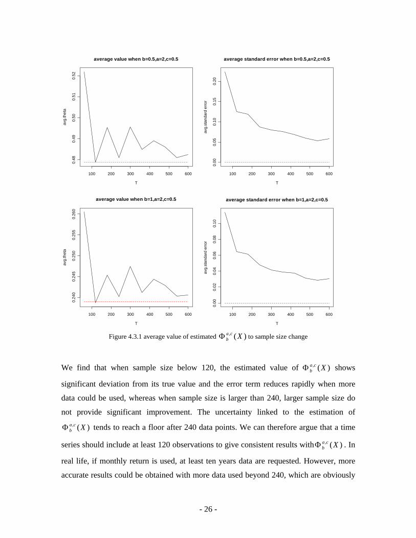
4.3 Estimation Risk In order to check estimation risk, we generate random variables with normal distribution,

where mean = 1 and standard deviation = 2. By varying the sample size from 60 to 600

data points, we simulate 100 returns time series for each sample size and compute their

values at six situations where different benchmarks and orders

( , /

)(, XcabΦ

1/5.0/0=b )2,( =ca )5.0,2( == ca ) are used. Then, we calculate the average value

of the estimated for each sample size at each situation. We also compute the

standard error of estimated around its true value, which is calculated by using

the parameter in the true distribution. This leads to Figure 4.3.1, the sensitivity of

estimated to sample size under different benchmarks and the orders is shown in

)(, XcabΦ

)(, XcabΦ

)(, XcabΦ

- 23 -

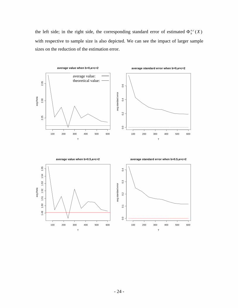
the left side; in the right side, the corresponding standard error of estimated

with respective to sample size is also depicted. We can see the impact of larger sample

sizes on the reduction of the estimation error.

)(, XcabΦ

100 200 300 400 500 600

2.25

2.30

2.35

average value when b=0,a=c=2

T

avg.

thet

a

100 200 300 400 500 600

0.0

0.2

0.4

0.6

average standard error when b=0,a=c=2

T

avg.

stan

dard

erro

r

average value: theoretical value:

100 200 300 400 500 600

1.49

1.50

1.51

1.52

1.53

1.54

1.55

average value when b=0.5,a=c=2

T

avg.

thet

a

100 200 300 400 500 600

0.0

0.1

0.2

0.3

0.4

average standard error when b=0.5,a=c=2

T

avg.

stan

dard

erro

r

- 24 -

100 200 300 400 500 600

0.99

51.

000

1.00

51.

010

1.01

51.

020

1.02

5

average value when b=1,a=c=2

T

avg.

thet

a

100 200 300 400 500 600

0.00

0.05

0.10

0.15

0.20

0.25

average standard error when b=1,a=c=2

T

avg.

stan

dard

erro

r

100 200 300 400 500 600

0.92

0.94

0.96

0.98

1.00

average value when b=0,a=2,c=0.5

T

avg.

thet

a

100 200 300 400 500 600

0.0

0.1

0.2

0.3

0.4

average standard error when b=0,a=2,c=0.5

T

avg.

stan

dard

erro

r

- 25 -

100 200 300 400 500 600

0.48

0.49

0.50

0.51

0.52

average value when b=0.5,a=2,c=0.5

T

avg.

thet

a

100 200 300 400 500 600

0.00

0.05

0.10

0.15

0.20

average standard error when b=0.5,a=2,c=0.5

T

avg.

stan

dard

erro

r

100 200 300 400 500 600

0.24

00.

245

0.25

00.

255

0.26

0

average value when b=1,a=2,c=0.5

T

avg.

thet

a

100 200 300 400 500 600

0.00

0.02

0.04

0.06

0.08

0.10

average standard error when b=1,a=2,c=0.5

T

avg.

stan

dard

erro

r

Figure 4.3.1 average value of estimated to sample size change )(, Xca

bΦ We find that when sample size below 120, the estimated value of shows

significant deviation from its true value and the error term reduces rapidly when more

data could be used, whereas when sample size is larger than 240, larger sample size do

not provide significant improvement. The uncertainty linked to the estimation of

tends to reach a floor after 240 data points. We can therefore argue that a time

series should include at least 120 observations to give consistent results with . In

real life, if monthly return is used, at least ten years data are requested. However, more

accurate results could be obtained with more data used beyond 240, which are obviously

)(, XcabΦ

)(, XcabΦ

)(, XcabΦ

- 26 -

shown in Figures 4.3.1, the right part; the standard error continues to decrease when

sample size is beyond 240.

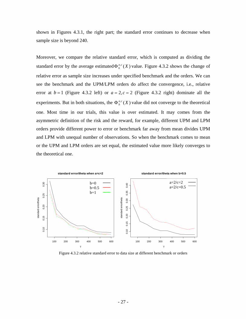
Moreover, we compare the relative standard error, which is computed as dividing the

standard error by the average estimated value. Figure 4.3.2 shows the change of

relative error as sample size increases under specified benchmark and the orders. We can

see the benchmark and the UPM/LPM orders do affect the convergence, i.e., relative

error at (Figure 4.3.2 left) or

)(, XcabΦ

1=b 2,2 == ca (Figure 4.3.2 right) dominate all the

experiments. But in both situations, the value did not converge to the theoretical

one. Most time in our trials, this value is over estimated. It may comes from the

asymmetric definition of the risk and the reward, for example, different UPM and LPM

orders provide different power to error or benchmark far away from mean divides UPM

and LPM with unequal number of observations. So when the benchmark comes to mean

or the UPM and LPM orders are set equal, the estimated value more likely converges to

the theoretical one.

)(, XcabΦ

100 200 300 400 500 600

0.10

0.15

0.20

0.25

0.30

standard error/theta when a=c=2

T

stan

dard

erro

r/the

ta

100 200 300 400 500 600

0.10

0.15

0.20

0.25

0.30

0.35

0.40

standard error/theta when b=0.5

T

stan

dard

erro

r/the

ta

a=2/c=2 a=2/c=0.5

b=0 b=0.5 b=1

Figure 4.3.2 relative standard error to data size at different benchmark or orders

- 27 -

5. Portfolio Optimization based on UPM/LPM framework Given the potential usefulness of UPM/LPM model, we expect it could be used in

portfolio selection. The optimization problem is,

{ }∑=

−⋅=k

i

aiiP XMAX

kLPMEMinimize

1

))(,0(1)( τωω

,

subject to

{ }∑=

=−⋅=k

ip

ciiP UPMXMAX

kUPME

1))(,0(1)( τω ,

11=⋅ω ,

or

{ }∑=

−⋅=k

t

ctt

TP XMAX

kUPMEMaximize

1))(,0(1)( τω

ω,

subject to

{ } p

k

t

att

TP LPMXMAX

kLPME =−⋅= ∑

=1

))(,0(1)( τω ,

11 =⋅Tω .

Where is the weight vector, ( nT ωωω L1= ) tnt xxX )( 1L= is the rate of return vector

during time t , and tτ is the benchmark during time t . We consider to do the portfolio

selection from n assets and simply get the expect value by averaging the values during

time period k . We are looking for a legitimate weight ( )nT ωωω L1= with minimal

downside risk given portfolio Upper Partial Moment or maximal upper potential

given downside risk . The weight vector

pUPM

pLPM ω is legitimate whenever it fulfills the

constraints.

If we want to check the efficient frontier of region, it can be found by

varying

LPMUPM /

λ and obtaining all the solutions to the problem as below,

- 28 -

)()( pP UPMELPMEMinimize λω

− ,

subject to

11 =⋅Tω .

In the following section, we will introduce an optimization method based on UPM/LPM

framework developed by Nawrocki, Moreno and Cumova (2004).

5.1 Optimization method

The and are reformulated as below, )( PUPME )( PLPME

∑∑∑∑≠= =

+==n

jiijjiii

n

i

n

jijjiP CLPMLPMCLPMLPME ωωωωω 2

1 1

)( ,

∑∑∑∑≠= =

+==n

jiijjiii

n

i

n

jijjiP CUPMPMUCUPMULPME ωωωωω 2

1 1

)( ,

where

{ }[ ]ak

titti xMAX

kLPM ∑

=

−=1

)(,01 τ , for , 1≥a

{ }[ ] )()(,01 1

1jtt

ak

tittij xxMAX

kCLPM −−=

−

=∑ ττ , for , 1>a

[ ]{ } )(11

).(0 jt

k

ttxMAXij xI

kCLPM

itT−⋅= ∑

=− ττ , for 1=a ,

{ }[ ]ck

ttiti xMAX

kUPM ∑

=

−=1

)(,01 τ , for , 1≥c

{ }[ ] )()(,01 1

1tjt

ck

ttitij xxMAX

kCUPM ττ −−=

−

=∑ , for 1>c

[ ]{ } )(11

).(0 tjt

k

txMAXij xI

kCUPM

Titττ −⋅= ∑

=− , for 1=c ,

- 29 -

iji CLPMLPM = ; iji CUPMUPM = , for any ji = .

Notice that under this formulation and are bounded for .

And for , otherwise,

)( pLPME )( pUPME 1, ≥ca

{ } 1=xI 0>x { } 0=xI . Unfortunately, the appropriate optimization

method for are still unknown. The general optimization problem is stated as

below,

1, <ca

ωωω

⋅⋅= LLPMMinimize Tp ,

subject to

UPMUUPM Tp =⋅⋅= ωω ,

bA =⋅ω ,

0≥ω ,

where

⎟⎟⎟

⎠

⎞

⎜⎜⎜

⎝

⎛=

nnn

n

CLPMCLPM

CLPMCLPML

L

MOM

L

1

111

,

⎟⎟⎟

⎠

⎞

⎜⎜⎜

⎝

⎛=

nnn

n

CUPMCUPM

CUPMCUPMU

L

MOM

L

1

111

,

⎟⎟⎟

⎠

⎞

⎜⎜⎜

⎝

⎛=

mnm

n

aa

aaA

L

MOM

L

1

111

,

)( 1 mT bbb L= .

Here A is the equality constraint matrix with rows for linear equalities constraints. m m

In this case, Lagrangian function is,

- 30 -

)21()(

21 UPMUbALL T

uTT −⋅⋅⋅−−⋅⋅−⋅⋅= ωωλωλωω ,

where and )( 1 mT λλλ L= uλ denote Lagrangian multipliers for constraints.

In order to obtain the efficient frontier in UPM/LPM region, we solve the following

optimization problem,

Pp UPMLPMMinimize ⋅− λω

,

subject to

bA =⋅ω ,

0≥ω .

By varying λ from 0 to ∞ , all sets of solutions compose the efficient frontier. For 0=λ ,

the global minimal portfolio is found, while ∞=λ the maximum portfolio is

found. The relationship is described in Figure 5.1.1

)(UPME

Figure 5.1.1 the relationship between λ and feasible set ),( LPMUPM

(source: Nawrocki, Moreno and Cumova (2004))

- 31 -

This reconstruction of and simplify the portfolio selection to a

quadratic optimization problem. To test if the weights obtained here are valid to construct

the efficient portfolio in the UPM/LPM region, we compare this frontier to the one

obtained from Markowitz MV optimization model in UPM/LPM region. Figure 5.1.2

shows a concave UPM/LPM frontier tracks alongside the MV frontier and dominates the

MV frontier almost all the time. Thus this method embodies the properties of UPM/LPM

model meanwhile it keeps the computation simplicity.

)( pLPME )( pUPME

0.05 0.10 0.15 0.20 0.25 0.30

1.0

1.5

2.0

2.5

efficient frontier

lpm(a=2)

upm

(c=2

)

0.1 0.2 0.3 0.4 0.5

0.8

1.0

1.2

1.4

efficient frontier

lpm(a=2)

upm

(c=1

)

Markowitz: UPM/LPM:

Figure 5.1.2 efficient frontier by UPM/LPM model and MV model 5.2 In-sample comparison When applying UPM/LPM model to portfolio optimization, we expect it could help to

manage higher moments of the portfolio return according to a specified investment

preference requirement. We generate ten groups of samples, 120 random variables of

each, with multivariate skewness student-t distribution. The statistic property of sample

set is listed in Table 5.2.1. We apply three different portfolio optimization models, based

on UPM/LPM framework, MV framework and mean-LPM framework, to these samples

and compare the allocation results as well as the statistics properties of the optimal

portfolios.

- 32 -

Mean SDev. Semi Dev Skewness Kurtosis Y1 0.66 1.03 0.73 0.02 3.94 Y2 0.49 0.95 0.70 -0.36 3.94 Y3 0.49 0.80 0.61 -0.58 4.31 Y4 0.66 0.93 0.61 0.50 3.89 Y5 0.85 1.55 1.15 -0.58 5.01 Y6 0.74 1.35 1.01 -0.45 3.84 Y7 0.61 1.34 0.97 -0.18 3.48 Y8 1.04 1.53 1.05 0.05 3.92 Y9 1.02 1.83 1.28 0.04 4.10 Y10 1.37 2.17 1.55 -0.17 6.01

Table 5.2.1 sample description

We focus on the global minimal risk portfolio, which is located in the extreme left of

efficient frontier. We obtain this portfolio by minimizing the risk without consideration

the reward level. Due to its independence of reward, we can isolate the influence of risk

definition on the portfolio allocation. Considering that the risk definitions under

UPM/LPM and mean-LPM framework are identical, we only compare the results from

UPM/LPM and MV model. In UPM/LPM approach, we obtain 4 portfolios by increasing

the order a from 1 to 4. Table 5.2.2 and Chart 5.2.1 describe the allocation results. It

clearly shows that MV portfolio prefers asset Y3, which has the smallest variance among

the ten assets, while as the order a increases, the UPM/LPM portfolio weighs more on

asset Y4, which has positive skewness.

- 33 -

MV LPM1 LPM2 LPM3 LPM4 Y1 0 0 0 0 0 Y2 0.267 0.1259 0.0318 0.0255 0.0241 Y3 0.4827 0.2679 0.3204 0.2708 0.2119 Y4 0.112 0.1051 0.3351 0.4893 0.5968 Y5 0 0.0162 0 0 0 Y6 0.0789 0.1655 0.1191 0.0794 0.0563 Y7 0.0594 0.057 0.0978 0.1019 0.1068 Y8 0 0 0 0 0 Y9 0 0.2011 0.0959 0.0332 0.004 Y10 0 0.0614 0 0 0

Table 5.2.2 asset allocation

Asset Allocation

00.10.20.30.40.50.60.7

MV LPM1 LPM2 LPM3 LPM4model selection

asse

t pro

porti

on

Y1Y2Y3Y4Y5Y6Y7Y8Y9Y10

Chart 5.2.1 asset allocation

The statistic properties of portfolio returns are presented in Table 5.2.3. It shows that the

MV global minimal risk portfolio has the lower standard deviation (SDev), while all

UPM/LPM global minimal risk portfolios except the one with 1=a have lower below

target standard deviation (SDt). It should not be a surprise since the variance is defined as

risk to be minimized in MV framework while the downside part is defined as risk in

UPM/LPM framework but with different orders. Among UPM/LPM portfolio, the LPM2

- 34 -

portfolio ( ) has the lowest SDt since in this case risk becomes the SVt; the LPM1

portfolio ( ) has a higher SDev and SDt consistent with the risk neutral attitude. The

major issue concerning the UPM/LPM framework is its capability to manage higher

moments. As the order a increase, the portfolio’s skewness increases. Moreover, the

portfolio skewness in LPM2, LPM3 and LPM4 are larger than the weighted sum of

individual asset skewness, which shows the ability of UPM/LPM model in managing

skewness.

2=a

1=a

MV LPM1 LPM2 LPM3 LPM4 Mean 0.5372 0.7231 0.6392 0.6227 0.6201

Standard Dev. 0.6436 0.8338 0.7257 0.7348 0.7602 Below Target SD 0.258 0.2995 0.2146 0.2181 0.2308

Skewness -0.448 0.0644 0.3173 0.3349 0.3505 Kurtosis 3.1246 4.4542 3.9764 3.8173 3.6994

Table 5.2.3 portfolio description

5.3 Efficient Frontier In order to analyze the relationship between risk and reward defined by MV, mean-LPM

and UPM/LPM framework, we compare their efficient frontiers in the following three

risk-reward coordinates,

• Mean-Standard deviation

• UPM/LPM( ): corresponding to risk aversion and potential seek 3,2=a =c

• UPM/LPM( ): corresponding to risk aversion and potential neutral 1,2 == ca

In the following experiments, we fix the benchmark 0=b .

- 35 -

0.7 0.8 0.9 1.0 1.1 1.2

0.6

0.7

0.8

0.9

efficient frontier

standard dev.

mea

n

MV: ULPM(a=2,c=3): ULPM(a=2,c=1): ULPM(a=1,c=2): MLPM(a=2):

Figure 5.3.1 efficient frontier in mean-variance coordinate

In the mean-standard deviation coordinate (Figure 5.3.1), the MV efficient frontier

dominates all the other frontiers. The closest frontier to the MV efficient frontier are the

ones from the UPM/LPM ( 1,2 == ca ) and the mean-LPM ( 2=a ) model, whose

objective function are closest to the MV framework, so are the downside part in their

utility functions. However, the UPM/LPM ( 1,2 == ca ) and the mean-LPM ( 2=a )

optimal portfolios sacrifice some efficiency in mean-standard deviation region by just

minimizing the SVt other than all the volatility deviating from the mean. The furthest

frontier from the MV efficient frontier is the one from the UPM/LPM ( 2,1 == ca )

model, for investors who are risk neutral and potential seek.

- 36 -

0.2 0.4 0.6 0.8 1.0

1.5

2.0

2.5

efficient frontier

lpm(a=2)

upm

(c=3

)

MV: ULPM(a=2,c=3): ULPM(a=2,c=1): ULPM(a=1,c=2): MLPM(a=2):

Figure 5.3.2 efficient frontier in UPM/LPM(a=2,c=3) coordinate In the UPM/LPM ( 3,2 == ca ) coordinate, it is as expected that the

UPM/LPM( ) optimal portfolios dominates all the other optimal portfolios

(Figure 5.3.2). The UPM/LPM (

3,2 == ca

3,2 == ca ), the mean-LPM ( ), and the

UPM/LPM ( ) model provides the same global minimal risk portfolio, because

both of them have the same risk definition, so does the utility function in the below

benchmark part. The furthest frontier from UPM/LPM (

2=a

1,2 == ca

3,2 == ca ) efficient frontier is

the one from UPM/LPM( 2,1 == ca ) model for investors who are risk neutral.

- 37 -

0.2 0.4 0.6 0.8 1.0

0.8

1.0

1.2

1.4

1.6

efficient frontier

lpm(a=2)

upm

(c=1

)

MV: ULPM(a=2,c=3): ULPM(a=2,c=1): ULPM(a=1,c=2): MLPM(a=2):

Figure 4.3.3 efficient frontier in UPM/LPM(a=2,c=1) coordinate When it comes to the UPM/LPM ( 1,2 == ca ) region, the frontier from UPM/LPM

( ), mean-LPM ( ) are similar as they do in the other cases, because they

have the similar optimization function for the similar utility functions.

1,2 == ca 2=a

5.4 Influence of Benchmark Shift Notice that in the UPM/LPM framework, a rise of benchmark b increases the risk

perception of an asset and reduces the reward perception. It is expected that the use of

different benchmarks should have an impact on portfolio selection. In order to investigate

the influence of benchmark shift on the efficient frontier, we contrast the efficient

frontiers obtained by increasing the benchmark from 0, 0.2 to 0.4 and leaving the other

parameters unchanged ( and 2=a 3=c / 2=a and 1=c ).

Recalling the congruent utility functions in UPM/LPM framework, benchmark b plays

as the kink point separating the attitudes towards lower part, downside risk, and upper

- 38 -

part, potential return. As it increases, the lower part to be minimized in portfolio

optimization increases and upper part decreases, so the efficient frontier would shift to

the down right direction in the corresponding UPM/LPM coordinate but to deferent

extent according to the order, which is shown in Figure 5.4.1.

0.2 0.4 0.6 0.8 1.0

510

1520

25

efficient frontier

lpm(a=2)

upm

(c=3

)

0.2 0.4 0.6 0.8 1.0

0.8

1.0

1.2

1.4

1.6

efficient frontier

lpm(a=2)

upm

(c=1

)

b=0: b=0.2: b=0.4:

Figure 5.4.1 efficient frontier change by the benchmark shift

Next, we check the influence of benchmark shift on global minimal risk portfolio. Here

we choose two different order set, 2=a and 3=c / 2=a and . The asset

allocation of these two global minimal risk portfolios are described in Table 5.4.1/Chart

5.4.1 and Table 5.4.2/ Chart 5.4.2. In both cases it could be observed that as benchmark

arises, asset Y2 and Y4 with relatively small semi-deviation are weighed more, while

asset Y7 with the largest semi-deviation among the selected assets is reduced. Moreover

the asset Y4 with positive skewness is weighed most in both portfolios.

1=c

b

- 39 -

GMP b=0 GMP b=0.2 GMP b=0.4 Y1 0 0.0053 0.0067 Y2 0.0318 0.0602 0.0791 Y3 0.3204 0.309 0.3044 Y4 0.3351 0.3538 0.3572 Y5 0 0 0 Y6 0.1191 0.1041 0.0942 Y7 0.0978 0.0752 0.052 Y8 0 0 0.0137 Y9 0.0959 0.0923 0.0927 Y10 0 0 0

Table 5.4.1 Global Minimal Risk Portfolio when b=0, 0.2, 0.4 (a=2, c=3)

Global Minimal Risk Portfolio Allocation

0

0.1

0.2

0.3

0.4

GMP b=0 GMP b=0.2 GMP b=0.4

Ass

et P

ropo

rtion

Y1Y2Y3Y4Y5Y6Y7Y8Y9Y10

Chart 5.4.1 Global Minimal Risk Portfolio when b=0, 0.2, 0.4 (a=2, c=3)

- 40 -

GMP b=0 GMP b=0.2 GMP b=0.4 Y1 0 0.0053 0.0067 Y2 0.0318 0.0602 0.0791 Y3 0.3204 0.309 0.3044 Y4 0.3351 0.3538 0.3572 Y5 0 0 0 Y6 0.1191 0.1041 0.0942 Y7 0.0978 0.0752 0.052 Y8 0 0 0.0137 Y9 0.0959 0.0923 0.0927 Y10 0 0 0

Table 5.4.2 Global Minimal Risk Portfolio when b=0, 0.2, 0.4 (a=2, c=1)

Global Minimal Risk Portfolio Allocation

0

0.1

0.2

0.3

0.4

GMP b=0 GMP b=0.2 GMP b=0.4

Ass

et P

ropo

rtion

Y1Y2Y3Y4Y5Y6Y7Y8Y9Y10

Table 5.4.2 Global Minimal Risk Portfolio when b=0, 0.2, 0.4 (a=2, c=1)

- 41 -

6. Conclusion UPM/LPM framework provides a new definition of risk and reward by lower partial

moment and upper partial moment. In this master thesis, we emphasize the importance of

UPM/LPM model to reflect investors’ asymmetric preferences in the investment decision

process and also show that the conventional frameworks are insufficient to adequately

assess the investment. In our empirical experiments for analyzing the properties of

UPM/LPM performance measurement, we find that it is able to incorporate higher

moments of portfolio returns in order to provide a custom ranking; by altering UPM/LPM

orders as well as benchmark the UPM/LPM performance index can rank portfolios

differently according to investors’ various preferences. Regarding to the estimation risk,

in the case of a normally distributed sample, at least 120 data is requested to obtain a

reliable performance analysis. When it is applied to portfolio optimization, we have

shown that compared to mean-variance and mean-lower partial moment models the

UPM/LPM model gives different allocation weights and a more efficient frontier in its

risk/reward region. In particularly, we apply the UPM/LPM model to multivariate

skewness student-t sample, and find that as investors become more risk averse it will

weigh more on the assets with less below-target variance or larger positive skewness.

- 42 -

References

1. Fishburn, Peter C., "Mean-Risk Analysis With Risk Associated With Below-

Target Returns", American Economic Review, 1977, v67(2), 116-126.

2. Harlow, W. V., "Asset Allocation In A Downside-Risk Framework", Financial

Analyst Journal, 1991, v47(5), 28-40.

3. Haugen, R., “Modern Investment Theory”, Prentice Hall, 1990.

4. Hogan, William W. and James, M. Warren., "Computation of The Efficient

Boundary In The E-S Portfolio Selection Model", Journal of Financial and

Quantitative Analysis, 1972, v7(4), 1881-1896.

5. Levy, H. and Markowitz, H. M., “Approximating Expected Utility by a Function

of Mean and Variance”, American Economic Review, Jun, 1979, Vol. 69 Issue 3,

p308, 10p.

6. Markowitz, H. M., "Portfolio Selection", Journal of Finance, 1952, v7(1), 77-91.

7. Markowitz, H. M., “Portfolio Selection: Efficient Diversification of Investments”,

John Wiley & Sons, Inc., 1959.

8. Markowitz, H. M.; Todd, P.; Xu, G.; Yamane, Y., “Computation of mean-

semivariance efficient sets by the Critical Line Algorithm”, Annals of operations

research, 1993, vol.45, No.1, 307.

9. Mao, J. C. T., “Models of Capital Budeting, E-V Vs E-S”, The Journal of

Financial and Quantitative Analysis, 1970, Vol. 4, No. 5 .

- 43 -

10. Moreno, D.; Cumova, D.; Nawrocki, D., “A Genetic Algorithm for UPM/LPM

portfolio”, Computing in Economics and Finance, 2006, No. 357.

11. Nash, S. G.; Sofer, A., “Linear And Nonlinear Programming”, The McGraw-Hill, 1996.

12. Nawrocki, D. N., "Optimal Algorithms And Lower Partial Moment: Ex Post

Results", Applied Economics, 1991, v23(3), 465-470.

13. Nawrocki, D. N., "The Characteristics of Portfolios Selected By n-Degree Lower

Partial Moment", International Review of Financial Analysis, 1992, v1(3), 195-

210.

14. Nawrocki, D. N., "A Brief History Of Downside Risk Measures", Journal of

Investing, 1999, v8 (3,Fall), 9-25.

15. Womersley, R.S. and Lau, K., “Portfolio Optimization Problems'', in A. Easton

and R. L. May eds., Computational Techniques and Applications , 1996, 795-802.

16. Sharpe, W. F., "Mutual Fund Performance", Journal of Business, 1966, v39(1),

Part II, 119-138.

17. Sortino, F. A. and Price, Lee N. "Performance Measurement in Downside Risk

Framework," Journal of Investing, 1994. (PRI website).

18. Sortino, F. A. and Forsey, H. J., "On The Use And Misuse Of Downside Risk",

Journal of Portfolio Management, 1996, v22(2,Winter), 35-42.

19. Sortino, F. A. and Kuan, B., “The U-P Strategy: A Paradigm Shift in Performance

Measurement”, Pension Research Institute, 1998.

- 44 -

20. Stoyanov, S.; Rachev, S.; Fabozzi, F., “Optimal Financial Portfolio”, Working

paper, Department of Probability and Applied Statistics, University of California,

Santa Barbara, USA, 2005.

21. Tibiletti, L. and Farinelli, S., "Sharpe Thinking with Asymmetrical Preferences",

Social Science Research Network, Oct. 2002.

- 45 -