the us model workbook
TRANSCRIPT
The US Model Workbook
Ray C. Fair
April 29, 2021


Contents
1 Introduction to Macroeconometric Models 71.1 Macroeconometric Models . . . . . . . . . . . . . . . . . . . . . . . . 71.2 Data . . . . . . . . . . . . . . . . . . . . . . . . . . . . . . . . . . . . 13
2 A Review of the US Model 152.1 History . . . . . . . . . . . . . . . . . . . . . . . . . . . . . . . . . . . 152.2 Tables of Variables and Equations . . . . . . . . . . . . . . . . . . . . 162.3 The Structure of the Model . . . . . . . . . . . . . . . . . . . . . . . . 162.4 Properties of the Model . . . . . . . . . . . . . . . . . . . . . . . . . . 222.5 Monetary Policy . . . . . . . . . . . . . . . . . . . . . . . . . . . . . . 272.6 Important Things to Know About the Program . . . . . . . . . . . . . . 31
3 Historical Data 37
4 NIPA and FFA Data 414.1 Identities . . . . . . . . . . . . . . . . . . . . . . . . . . . . . . . . . . 414.2 Nominal versus Real GDP . . . . . . . . . . . . . . . . . . . . . . . . 424.3 Federal Government Variables . . . . . . . . . . . . . . . . . . . . . . 434.4 Financial Saving . . . . . . . . . . . . . . . . . . . . . . . . . . . . . . 43
5 Fiscal Policy Effects 475.1 Changes in Government Purchases of Goods . . . . . . . . . . . . . . . 475.2 Other Fiscal Policy Variables . . . . . . . . . . . . . . . . . . . . . . . 49
6 Monetary Policy Effects 55
7 Price Shocks and Stock Market Shocks 577.1 Price Shocks . . . . . . . . . . . . . . . . . . . . . . . . . . . . . . . . 577.2 Stock Market Shocks . . . . . . . . . . . . . . . . . . . . . . . . . . . 59
8 Housing Price Shocks 61
3
4
9 Fed’s Weight on Inflation 63
10 Interest Elasticity of Aggregate Expenditures 65
11 Specification of the Price Equation 67
12 Foreign Sector Effects 69
13 Other Possible Experiments 7113.1Combinations of Policies . . . . . . . . . . . . . . . . . . . . . . . . . 7113.2Effects of Changing State and Local Government Variables . . . . . . . 7213.3Imposing Rational Expectations on the Model . . . . . . . . . . . . . . 7213.4Making Major Changes to the Model . . . . . . . . . . . . . . . . . . . 7413.5Supply Side Experiments . . . . . . . . . . . . . . . . . . . . . . . . . 7413.6Counterfactual Experiments . . . . . . . . . . . . . . . . . . . . . . . . 75
Preface
This workbook can be used at a variety of levels. Chapter 1 contains introductorymaterial. It presents the vocabulary of model building and covers the main issues thatare involved in constructing and working with macroeconometric models. Chapter 2is a review of the US model, and you should definitely look over this chapter beforebeginning to do the experiments. Some of the material in Chapter 2 is intermediateor advanced, but it can be easily skipped by introductory users.
The experiments begin in Chapter 3. The experiments in Chapter 3 are descriptive,and these can be very useful for introductory students. The experiments give studentsa feel for the data, especially for how variables change over time. All of Chapter 3 isintroductory. Chapter 4 is also introductory; it contains descriptive experiments aboutthe National Income and Product Accounts (NIPA) and the Flow of Funds Accounts(FFA).
The analysis begins in Chapter 5, where fiscal-policy effects are examined. Thismaterial is accessible to introductory students who have had the equivalent of theIS-LM model. (Although most introductory texts do not refer to the model that theyare teaching as the“IS-LM” model, this is in fact the model that they are using.) Thefirst two experiments pertain to changing government spending under two differentassumptions about monetary policy. The rest of the experiments in this chapter pertainto changing other fiscal-policy variables, and this can be skipped by introductory usersif desired.
Chapter 6 discusses monetary-policy effects, namely the effects of changing theshort term interest rate, and again this material is accessible to those who have hadthe equivalent of the IS-LM model.
The first part of Chapter 7 discusses price shocks, and this material is accessibleto those who have had the equivalent of the AS-AD model. The first two experimentsconcern changing the import price index, PIM , and these changes can be lookedupon as shifts of the AS curve. Both of these experiments are good ways of showinghow stagflation can arise. The second part of Chapter 7 examines wealth effectsthrough stock market shocks, and this is intermediate material.
5
6
Chapter 8 is also intermediate material. It examines the effects on the economyof changing housing prices.
Chapters 9-13 are intermediate to advanced. Many of the experiments requirechanging coefficients in the equations and examining how the properties of the modeldiffer for these changes. At the intermediate level this is an excellent way of gettingstudents to have a deeper understanding of macroeconomic issues. The suggestionsin Chapter 13 about imposing rational expectations on the model and making majorchanges to the model are for advanced users.
To summarize, the following is recommended for introductory users:
1. Chapter 1 - read carefully
2. Chapter 2 - look over and then use for reference purposes
3. Chapter 3 - do all the experiments
4. Chapter 4 - do all the experiments
5. Chapter 5 - do at least the first two experiments
6. Chapter 6 - do the experiment
7. Chapter 7 - do the first two experiments
Everything in the workbook is accessible to intermediate users except perhaps forSections 13.3 and 13.4.
The latest version of the US model is dated April 29, 2021. I has been estimatedthrough 2021:1. The estimates of this version are presented in The US Model AppendixA: April 29, 2021. A complete discussion of the version of the US model dated January28, 2018, is in Macroeconometric Modeling. A few changes have been made to themodel beginning with the April 29, 2021, version. These are listed in The US ModelAppendix C: April 29, 2021.
Macroeconometric Modeling should be read by those contemplating using themodel for research. This reference may also be of interest to teachers who would likea deeper understanding of the model than can be obtained by reading Chapter 2 ofthis workbook. There are a number of experiments in Macroeconometric Modelingthat may be of interest to discuss with advanced students.
Chapter 1
Introduction to MacroeconometricModels
1.1 Macroeconometric Models
A macroeconometric model like the US model is a set of equations designed toexplain the economy or some part of the economy. There are two types of equations:stochastic, or behavioral, and identities. Stochastic equations are estimated from thehistorical data. Identities are equations that hold by definition; they are always true.
There are two types of variables in macroeconometric models: endogenous andexogenous. Endogenous variables are explained by the equations, either the stochas-tic equations or the identities. Exogenous variables are not explained within themodel. They are taken as given from the point of view of the model. For example,suppose you are trying to explain consumption of individuals in the United States.Consumption would be an endogenous variable-a variable you are trying to explain.One possible exogenous variable is the income tax rate. The income tax rate is setby the government, and if you are not interested in explaining government behavior,you would take the tax rate as exogenous.
Specification
It is easiest to consider what a macroeconometric model is like by considering asimple example. The following is a simple multiplier model. Ct is consumption, Itis investment, Yt is total income or GDP, Gt is government spending, and rt is theinterest rate. The t subscripts refer to period t.
Ct = α1 + α2Yt + et, (1)
7

8 CHAPTER 1. INTRODUCTION TO MACROECONOMETRIC MODELS
It = β1 + β2rt + ut, (2)
Yt = Ct + It +Gt, (3)
Equation (1) is the consumption function, equation (2) is the investment function, andequation (3) is the income identity. Equations (1) and (2) are stochastic equations,and equation (3) is an identity. The endogenous variables are Ct, It, and Yt; they areexplained by the model. rt and Gt are exogenous variables; they are not explained.
The specification of stochastic equations is based on theory. Before we write downequations (1) and (2), we need to specify what factors we think affect consumption andinvestment in the economy. We decide these factors by using theories of consumptionand investment. The theory behind equation (1) is simply that households decide howmuch to consume on the basis of their current income. The theory behind equation(2) is that firms decide how much to invest on the basis of the current interest rate. Inequation (1) consumption is a function of income, and in equation (2) investment is afunction of the interest rate. The theories behind these equations are obviously muchtoo simple to be of much practical use, but they are useful for illustration. In practiceit is important that we specify our equations on the basis of a plausible theory. Forexample, we could certainly specify that consumption was a function of the numberof sunny days in period t, but this would not be sensible. There is no serious theoryof household behavior behind this specification.
et and ut are error terms. The error term in an equation encompasses all the othervariables that have not been accounted for that help explain the endogenous variable.For example, in equation (1) the only variable that we have explicitly stated affectsconsumption is income. There are, of course, many other factors that are likely toaffect consumption, such as the interest rate and wealth. There are many reasons thatnot all variables can be included in an equation. In some cases data on a relevantvariable may not exist, and in other cases a relevant variable may not be known tothe investigator. We summarize the effects of all of the left out variables by addingan error term to the equation. Thus, the error term et in equation (1) captures all thefactors that affect consumption other than current income. Likewise, the error termut in equation (2) captures all the factors that affect investment other than the interestrate.
Now, suppose that we were perfectly correct in specifying that consumption issolely a function of income. That is, contrary to above discussion, suppose there wereno other factors that have any influence on consumption except income. Then theerror term, et, would equal zero. Although this is unrealistic, it is clear that one hopesthat consumption in each period is mostly explained by income. This would meanthat the other factors explaining consumption do not have a large effect, and so theerror term for each period would be small. This means that the variance of the errorterm would be small. The smaller the variance, the more has been explained by the

1.1. MACROECONOMETRIC MODELS 9
explanatory variables in the equation. The variance of an error term is an estimate ofhow much of the left hand side variable has not been explained. In macroeconomics,the variances are never zero; there are always factors that affect variables that are notcaptured by the stochastic equations.
Equation (3), the income identity, is true regardless of the theories one has forconsumption and investment. Income is always equal to consumption plus investmentplus government spending (we are ignoring exports and imports here).
Estimation
Once stochastic equations have been specified (written down), they must be estimatedif they are to be used in a model. Theories do not tell us the size of coefficients likeα1, α2, β1, and β2. These coefficients must be estimated using historical data. Giventhe data and the specification of the equations, the estimation techniques choose thevalues of the coefficients that best“fit” the data in some sense.
Consider the consumption equation above. One way to think of the best fit of thisequation is to graph the observations on consumption and income, with consumptionon the vertical axis and income on the horizontal axis. You can then think of the bestfit as trying to find the equation of the line that is“closest to” the data points, whereα2 would be the slope of the line and α1 would be the intercept. The ordinary leastsquares technique picks the line that minimizes the sum of the squared deviations ofeach observation to the line.
A common estimation technique in macroeconometrics is two-stage least squares,which is the technique used to estimate the US model. This technique is similar to theordinary least squares technique except that it adjusts for certain statistical problemsthat arise when there are endogenous variables among the explanatory (right handside) variables. In our current example, one would estimate the four coefficients α1,α2, β1, and β2.
Solution
Once a model has been specified and estimated, it is ready to be solved. By “solving”a model, we mean solving for the values of the endogenous variables given valuesfor the exogenous variables. Remember that exogenous variables are not explainedwithin the model. Say that we are in period t − 1 and we want to use the modelto forecast consumption, investment, and income for period t. We must first choosevalues of government spending and the interest rate for period t. Since t is in the future,we do not know for certain what government spending and the interest rate will be inperiod t, and so we must make our best guesses based on available information. (Forexample, we might use projected government budgets.) In other words, our model
10 CHAPTER 1. INTRODUCTION TO MACROECONOMETRIC MODELS
forecasts what consumption, investment, and income will be in period t if the valueswe chose for government spending and the interest rate in period t are correct. Wemust also choose values for the error terms for period t, which in most cases aretaken to be zero. Given the exogenous variable values, the values of the error terms,and the coefficient estimates, equations (1), (2), and (3) are three equations in threeunknowns, the three unknowns being the three endogenous variables, Ct, It, and Yt.Thus, the model can be solved to find the three unknowns.
A model like equations (1)-(3) is called simultaneous. Income is an explanatoryvariable in the consumption function, and consumption is a variable in the incomeidentity. One cannot calculate consumption from equation (1) unless income is known,and one cannot calculate income from equation (3) unless consumption is known. Wethus say that consumption and income are“simultaneously” determined. (Investmentin this model is not simultaneously determined because it can be calculated once thevalue for the exogenous variable rt has been chosen.)
The above model, even though it is simultaneous, is easy to solve by simplysubstituting equations (1) and (2) into (3) and solving the resulting equation for Yt.Once Yt is solved, Ct can then be solved. In general, however, models are not thissimple, and in practice models are usually solved numerically using the Gauss-Seideltechnique. The steps of the Gauss-Seidel technique are as follows:
1. Guess a set of values for the endogenous variables.
2. Using this set of values for the right hand side variables, solve all the equationsfor the left hand side variables.
3. Step 2 yields a new set of values of the endogenous variables. Replace theinitial set with this new set, and solve for the left hand side variables again.
4. Keep replacing the previous set of values with the new set until the differencesbetween the new set and the previous set are within the required degree ofaccuracy. When the required accuracy has been reached,“convergence” hasbeen attained, and the model is solved. The right hand side values are consistentwith the computed left hand side values.
If a variable computed by an equation is used on the right hand side of an equationthat follows, usually the newly computed value is used rather than the value from theprevious iteration. It is not necessary to do this, but it usually speeds convergence.The usual procedure for the above model would be to guess a value for Yt, computeCt from equation (1) and It from equation (2), and use the computed values to solvefor Yt in equation (3). This new value of Yt would then be used for the next passthrough the model.

1.1. MACROECONOMETRIC MODELS 11
Testing
Once a model has been specified and estimated, it is ready to be tested. Testingalternative models is not easy, and this is one of the reasons there is so much dis-agreement in macroeconomics. The testing of models is discussed extensively inMacroeconometric Modeling, and the interested reader is referred to this material.
One obvious and popular way to test a model is to see how close its predictedvalues are to the actual values. Say that you want to know how well the modelexplained output and inflation in the 1970s. Given the actual values of the exogenousvariables over this period, the model can be solved for the endogenous variables. Thesolution values of the endogenous variables are the predicted values. If the predictedvalues of output and inflation are close to the actual values, then we can say that themodel did a good job in explaining output and inflation in the 1970s; otherwise not.
The solution of a model over a historical period, where the actual values of theexogenous variables are known, is called an ex post simulation. In this case, we donot have to guess values of the exogenous variables because all of these variables areknown. One can thus use ex post simulations to test a model in the sense of examininghow well it predicts historical episodes.
Forecasting
Once a model has been specified and estimated, it can be used to forecast the future.Forecasts into the future require that one first choose future values of the exogenousvariables, as we described in the Solution section above. Given values of the exoge-nous variables, we can solve for the values of the endogenous variables. The solutionof a model for a future period, where“guessed” values of the exogenous variables areused, is called an ex ante simulation.
Analyzing Properties of Models
Perhaps the most important use of a model is to try to learn about the properties ofthe economy by examining the properties of the model. If a model is an adequaterepresentation of the economy, then its properties should be a good approximation tothe actual properties of the economy. One may thus be able to use a model to get agood idea of the likely effects on the economy of various monetary and fiscal policychanges.
In the simple model above there are two basic questions that can be asked aboutits properties. One is how income changes when government spending changes, andthe other is how income changes when the interest rate changes. In general one asksthe question of how the endogenous variables change when one or more exogenous
12 CHAPTER 1. INTRODUCTION TO MACROECONOMETRIC MODELS
variables change. Remember, in our simple model above the only exogenous variablesare government spending and the interest rate.
The Gauss-Seidel technique can be used to analyze a model’s properties. Considerthe question of how Yt changes whenGt changes in the above model. In other words,one would like to know how income in the economy is affected when the governmentchanges the amount that it spends. One first solves the model for a particular valueof Gt (and rt), perhaps the historical value of Gt if the value for period t is known.Let Y ∗t be the solution value of Yt. Now change the value ofGt (but not rt) and solvethe model for this new value. Let Y ∗∗t be this new solution value. Then Y ∗∗t − Y ∗tis the change in income that has resulted from the change in government spending.(The change in Y divided by the change in G is sometimes called the“multiplier,”hence the name of the model.) Similarly, one can examine how income changes whenthe interest rate changes by 1) solving the model for a given value of rt, 2) solvingthe model for a new value of rt, and 3) comparing the predicted values from the twosolutions. You can begin to see how all sorts of proposed policies can be analyzed asto their likely effects if you have a good macroeconometric model.
Most of the experiments in this workbook are concerned with examining the prop-erties of the US model. You will be comparing one set of solution values with another.If you understand these properties and if the model is an adequate approximation ofthe economy, then you will have a good understanding of how the economy works.
Further Complications
Actual models are obviously more complicated than equations (1)–(3) above. Forone thing, lagged endogenous variables usually appear as explanatory variables ina model. The value of consumption in period t − 1, denoted Ct−1, is a lagged en-dogenous variable since it is the lagged value ofCt, which is an endogenous variable.If Ct−1 appeared as an explanatory variable in equation (1), then the model wouldinclude a lagged endogenous variable.
When lagged endogenous variables are included in a model, the model is said tobe dynamic. An important feature of a dynamic model is that the predicted values inone period affect the predicted values in future periods. What happens today affectswhat happens tomorrow, and the model is dynamic in this sense. Again, in the case ofconsumption, the idea is that how much you decide to consume this year will affecthow much you decide to consume next year.
Also, most models in practice are nonlinear, contrary to the above model, where,for example, consumption is a linear function of income in equation (1). In particular,most models include ratios of variables and logarithms of variables. Equation (1), for
1.2. DATA 13
example, might be specified in log terms:
logCt = α1 + α2 log Yt + et, (1)′
Nonlinear models are difficult or impossible to solve analytically, but they can usuallybe solved numerically using the Gauss-Seidel technique. The same kinds of experi-ments can thus be performed for nonlinear models as for linear models. As long as amodel can be solved numerically, it does not really matter whether it is nonlinear ornot for purposes of forecasting and policy analysis.
The error terms in many stochastic equations in macroeconomics appear to becorrelated with their past values. In particular, many error terms appear to be firstorder serially correlated. If et is first order serially correlated, this means that:
et = ρet−1 + vt,
where ρ is the first order serial correlation coefficient and vt is an error term that is notserially correlated. In the estimation of an equation one can treat ρ as a coefficient tobe estimated and estimate it along with the other coefficients in the equation. This isdone for a number of the stochastic equations in the US model.
1.2 Data
It is important in macroeconomics to have a good understanding of the data. Macroe-conomic data are available at many different intervals. Data on variables like interestrates and stock prices are available daily; data on variables like the money supply areavailable weekly; data on variables like unemployment, retail sales, and industrialproduction are available monthly; and variables from the NIPA and FFA are availablequarterly. It is always possible, of course, to create monthly variables from weeklyor daily variables, quarterly variables from monthly variables, and so on.
The US model is a quarterly model; all the variables are quarterly. An importantpoint should be kept in mind when dealing with quarterly variables. In most casesquarterly variables are quoted at seasonally adjusted annual rates. For example, inthe NIPA real GDP for the fourth quarter of 1994 is listed as $10352.4 billion, butthis does not mean that the U.S. economy produced $10352.4 billion worth of outputin the fourth quarter. First, the figure is seasonally adjusted, which means that it isadjusted to account for the fact that on average more output is produced in the fourthquarter than it is in the other three quarters. The number before seasonal adjustmentis higher than the seasonally adjusted number. Seasonally adjusting the data smoothsout the ups and downs that occur because of seasonal factors.
Second, the figure of $10352.4 billion is also quoted at an annual rate, whichmeans that it is four times larger than the amount of output actually produced (ignoring

14 CHAPTER 1. INTRODUCTION TO MACROECONOMETRIC MODELS
seasonal adjustment). Being quoted at an annual rate means that if the rate of outputcontinued at the rate produced in the quarter for the whole year, the amount of outputproduced would be $10352.4 billion. For variables that are quoted at annual rates,it is not the case that the yearly amount is the sum of the four published quarterlyamounts. The yearly amount is one fourth of this sum, since all the quarterly amountsare multiplied by four.
In the US model all variables are seasonally adjusted when appropriate and allflow variables are at quarterly rates. If you want to examine the flow variables atannual rates, just multiply by four.
It is also important to understand how growth rates are computed. Consider avariable Yt. The change in Y from period t − 1 to period t is Yt − Yt−1. Thepercentage change in Y from t− 1 to t is (Yt − Yt−1)/Yt−1, which is the change inY divided by Yt−1. If, for example, Yt−1 is 100 and Yt is 101, the change is 1 andthe percentage change is .01. The percentage change is usually quoted in percentagepoints, which in the present example means that .01 would be multiplied by 100 tomake it 1.0 percent.
The percentage change in a variable is also called the growth rate of the variable,except that in most cases growth rates are given at annual rates. In the present example,the growth rate of Y at an annual rate in percentage points is
GrowthRate(annualrate) = 100[(Yt/Yt−1)4 − 1]
If Yt−1 is 100 and Yt is 101, the growth rate is 4.06 percent. Note that this growth rateis slightly larger than four times the quarterly growth rate of 1.0 percent. The aboveformula “compounds” the growth rate, which makes it slightly larger than 4 percent.The growth rate at an annual rate is the rate that the economy would grow in a year ifit continued to grow at the same rate in the next three quarters as it did in the currentquarter.

Chapter 2
A Review of the US Model
2.1 History
The US model consists 25 stochastic equations and slightly over 100 identities. Thereare about 150 exogenous variables and many lagged endogenous variables. Thestochastic equations are estimated by two-stage least squares. The data base for themodel begins in the first quarter of 1952.
Work began on the theoretical basis of the model in 1972. The theoretical workstressed three ideas: 1) basing macroeconomics on solid microeconomic foundations,2) allowing for the possibility of disequilibrium in some markets, and 3) accountingfor all balance sheet and flow of funds constraints. The stress on microeconomicfoundations for macroeconomics has come to dominate macro theory, and this workin the early 1970s is consistent with the current emphasis. The introduction of dise-quilibrium possibilities in some markets provides an explanation of business cyclesthat is consistent with maximizing behavior. The model explains disequilibrium onthe basis of non rational expectations. Agents must form expectations of the futurevalues of various variables before solving their multiperiod maximization problems.It is assumed that no agent knows the complete model, and so expectations are notrational. Firms, for example, make their price and wage decisions based on expec-tations that are not rational, which can cause disequilibrium in the goods and labormarkets.
The theoretical model was used to guide the specification of the econometricmodel. This work was done in 1974 and 1975, and by 1976 the model was essentiallyin the form that it is in today. The explanatory variables in the econometric model werechosen to be consistent with the assumption of maximizing behavior, and an attemptwas made to model the effects of disequilibrium. Balance sheet and flow of fundsconstraints were accounted for: the NIPA and FFA data are completely integrated
15
16 CHAPTER 2. A REVIEW OF THE US MODEL
in the model. This latter feature greatly helps in considering alternative monetarypolicies, and it allows one to consider carefully“crowding out” questions.
2.2 Tables of Variables and Equations
An attempt has been made in this workbook to have nothing in the model be a “blackbox,” including the collection of the data. This has been done by putting the completelisting of the model and the data collection in The US Model Appendix A: April 29,2021. The hope is that with a careful reading of the tables in Appendix A, you cananswer why the model has the particular properties that it has. You should use thesetables for reference purposes.
Table A.1 presents the six sectors in the US model: household (h), firm (f),financial (b), foreign (r), federal government (g), and state and local government (s).In order to account for the flow of funds among these sectors and for their balance-sheet constraints, the U.S. Flow of Funds Accounts (FFA) and the U.S. NationalIncome and Product Accounts (NIPA) must be linked. Many of the identities in theUS model are concerned with this linkage. Table A.1 shows how the six sectors inthe US model are related to the sectors in the FFA. The notation on the right side ofthis table (H1, FA, etc.) is used in Table A.5 in the description of the FFA data.
Table A.2 lists all the variables in the US model in alphabetical order, and TableA.3 lists all the stochastic equations and identities. Table A.2 also lists which variablesappear in which equations, which can be useful for tracing through how one variable beaffects other variables in the model. The functional forms of the stochastic equationsare given in Table A.3, but not the coefficient estimates. The coefficient estimates arepresented in Table A.4, where within this table the coefficient estimates and tests forequation 1 are presented in Table A1, for equation 2 in Table A2, and so on. The testsfor the equations, which are reported in Table A.4, are explained in MacroeconometricModeling, and this discussion is not presented in this workbook.
The remaining tables provide more detailed information about the model. TablesA.5-A.7 show how the variables were constructed from the raw data. Table A.9 liststhe first stage regressors per equation that were used for the two-stage least squaresestimates.
2.3 The Structure of the Model
The model is divided into six sectors:
1. Household sector (h)
2. Firm sector (f)

2.3. THE STRUCTURE OF THE MODEL 17
3. Financial sector (b)
4. Federal government sector (g)
5. State and local government sector (s)
6. Foreign sector (r)
Each of these sectors will be discussed in turn.
The Household Sector
In the multiplier model in Chapter 1, consumption is simply a function of currentincome, but this is obviously much too simple as a description of reality. As notedabove, the stress in the model is on microeconomic foundations and possible dise-quilibrium effects. In the microeconomic story households maximize a multiperiodutility function. Households make two decisions each period. They decide how muchto consume and how many hours to work. If households can work as many hours asthey wish (no disequilibrium), then income, which is the wage rate times the numberof hours worked, is not an appropriate explanatory variable in a consumption equa-tion, because part of it (the number of hours worked) is itself a decision variable. Ifthere is no disequilibrium, decisions about consumption and hours worked are madeat the same time. Households do not earn income and then decide how much toconsume. Consumption and hours worked are instead determined jointly, and hoursworked should not be considered as helping to ”explain” consumption if there is nodisequilibrium. Both variables are ”explained” by other variables.
The main variables that explain consumption and hours worked in the microeco-nomic story are the wage rate, the price level, the interest rate, tax rates, the initialvalue of wealth, and nonlabor income. The interest rate affects consumption becauseof the multiperiod nature of the maximization problem. This microeconomic storyhas to be modified if households are not allowed to work as many hours as theywould like. If households want to work more hours than firms want to employ and iffirms employ only the amount they want (which seems reasonable), then householdsare“constrained” from working their desired number of hours. These periods corre-spond to periods of“unemployment.” The existence of binding labor constraints islikely to lead households to consume less than they otherwise would. Also, a bindinglabor constraint on a household means that income is a legitimate explanatory variablefor consumption, since the number hours worked is no longer a decision variable. Itis imposed from the outside by firms. As discussed below, an attempt has been madein the econometric work to handle possible disequilibrium effects within the contextof the microeconomic story.
18 CHAPTER 2. A REVIEW OF THE US MODEL
In the empirical work the expenditures of the household sector are disaggregatedinto four types: consumption of services (CS), consumption of nondurable goods(CN ), consumption of durable goods (CD), and investment in housing (IHH).Four labor supply variables are used: the labor force of men 25–54 (L1), the laborforce of women 25–54 (L2), the labor force of all others 16+ (L3), and the number ofpeople holding more than one job, called“moonlighters” (LM ). These eight variablesare determined by eight estimated equations.
There are two main empirical approaches that can be taken regarding the use ofwage, price, and income variables in the consumption equations. The first is to addthe wage, price, nonlabor income, and labor constraint variables separately to theequations. These variables in the model are as follows. The after tax nominal wagerate isWA, the price deflator for total household expenditures is PH , and the beforetax nonlabor income variable is Y NL. The price deflators for the four expenditurecategories are PCS, PCN , PCD, and PIH .
Regarding a labor constraint variable, let Z denote a variable that takes on a valueof zero when there is no binding labor constraint (periods of full employment) andvalues further and further below zero as the economy gets further and further from fullemployment. (In earlier versions of the US model there was such a variable.) Consideras an example the CS equation. Under the first approach one might add WA/PH ,PCS/PH , Y NL/PH , and Z to the equation. The justification for including Z isthe following. By construction, Z is zero or nearly zero in tight labor markets. In thiscase the labor constraint is not binding and Z has no effect or only a small effect inthe equation. This is the ”classical” case. As labor markets get looser, on the otherhand, Z falls and begins to have an effect in the equation. Loose labor markets, whereZ is large in absolute value, correspond to the “Keynesian” case. Since Z is highlycorrelated with hours paid for in loose labor markets, having both WA and Z in theequation is similar to having a labor income variable in the equation in loose labormarkets.
The second, more traditional, empirical approach is to replace the above fourvariables with real disposable personal income, Y D/PH . This approach in effectassumes that labor markets are always loose and that the responses to changes in laborand nonlabor income are the same. One can test whether the data support Y D/PHover the other variables by including all the variables in the equation and examiningtheir significance. The results of doing this in the four expenditure equations supportsthe use of Y D/PH over the other variables, and so the equations that are chosen forthe model use Y D/PH .
The dominance of Y D/PH does not necessarily mean that the classical casenever holds in practice. What it does suggest is that trying to capture the classicalcase through the use of Z does not work. An interesting question for future work iswhether the classical case can be captured in some other way.

2.3. THE STRUCTURE OF THE MODEL 19
The first eight equations in Table A.4 in Appendix A are for the household sector.As noted above, there are four expenditure equations and four labor supply equations.These are the first eight equations in Table A.4.
The Firm Sector
There are nine stochastic equations for the firm sector (equations 10 through 18in Table A.4). The firm sector determines production given sales (i.e., inventoryinvestment), nonresidential fixed investment, employment demand, the price level,and the wage rate, among other things.
In the multiplier model in Chapter 1 investment is only a function of the interestrate. There is no labor market, and so employment demand is not determined. Also,no distinction is made between production and sales, and so there is no inventoryinvestment. (Inventory investment in a period is the difference between what firmsproduce and what they sell.) Finally, no mention is made as to how the price levelis determined. A realistic model of the economy must obviously take into accountmore features of firm behavior.
Production in the model is a function of sales and of the lagged stock of inventories(equation 11). Production is assumed to be ”smoothed” relative to sales.
The capital stock of the firm sector depends on the amount of excess capital onhand and on current and lagged values of output (equation 12). It also depends ontwo cost of capital variables: a real interest rate variable and a stock market variable.Nonresidential fixed investment is determined by an identity (equation 92). It is equalto the change in the capital stock plus depreciation. The demand for workers and hoursdepends on output and the amount of excess labor on hand (equations 13 and 14).(Excess labor is labor that the firm holds (pays for) that is not needed to produce thecurrent level of output.)
The price level of the firm sector is determined by equation 10. It is a functionof the lagged price level, the wage rate, the price of imports, the unemployment rate,and a time trend. The lagged price level is meant to pick up expectational effects, theunemployment rate is meant to pick up demand pressure effects, and the wage rateand import price variables are meant to pick up cost effects.
The nominal wage of the firm sector is determined by equation 16. The nominalwage rate is a function of the current and lagged value of the price level. The equationis best thought of as a real wage equation, where the nominal wage rate adjusts tothe price level with a lag. Equation 17 determines the demand for money of the firmsector. It is discussed later.
The other stochastic equations for the firm sector are fairly minor. The level ofovertime hours is a nonlinear function of total hours (equation 15). The level ofdividends paid is a function of after tax profits (equation 18).
20 CHAPTER 2. A REVIEW OF THE US MODEL
The Financial Sector
The multiplier model in Chapter 1 is the IS part of the IS-LM model. The LM part ofthis model is as follows:
Mdt /Pt = d1 + d2Yt + d3rt + wt, (4)
M st = Mt, (5)
Mdt = M s
t , (6)
whereMdt is the quantity of money demanded,M s
t is the quantity of money supplied,and Pt is the price level. In equation (4) the demand for real money balances is afunction of income and the interest rate. Equation (5) states that the supply of moneyis equal to Mt, which is assumed to be the policy variable of the monetary authority.Equation (6) is the equilibrium condition in the money market; the money marketis assumed to clear—the quantity of money demanded equals the quantity of moneysupplied. The three endogenous variables in equations (4)-(6) are Md
t , Mdt , and rt.
The exogenous variables to this block of equations are Mt, Yt, and Pt.When equations (4)-(6) are added to equations (1)-(3) in Chapter 1, Yt, which is
exogenous in the LM model, becomes endogenous and rt, which is exogenous in theIS model, becomes endogenous. The exogenous variables in this expanded model,the overall IS-LM model, are Gt, Mt, and Pt.
The demand for money equations in the model are consistent with equation (4)of the LM model. The main demand for money equation is for the firm sector—equation 17. In this equation the demand for money is a function of the interest rateand a transactions variable. There is also a separate demand for currency equation—equation 26—which is similar to equation 17.
An important difference between the present model and the LM model is that thepresent model accounts for all the flows of funds among the sectors and all balancesheet constraints. This allows the main“tool” of the monetary authority in the modelto be open market operations, which is the main tool used in practice.
The other equations of the financial sector consist two term structure equationsand an equation explaining the change in stock prices. The bond rate in the first termstructure equation is a function of current and lagged values of the bill rate (equation23). The same is true for the mortgage rate in the second term structure equation(equation 24). In the stock price equation, the change in stock prices is a function ofthe change in the bond rate and the change in after tax profits (equation 25).
The Foreign Sector
There is one stochastic equation in the foreign sector, which explains the level ofimports (equation 27). The level of imports depends on income, wealth, and the

2.3. THE STRUCTURE OF THE MODEL 21
domestic price level relative to the price of imports. If the price of imports rises relativeto the domestic price level, imports are predicted to fall, other things being equal, aspeople substitute domestic goods for imported goods. Otherwise, the variables in theimport equation are similar to those in the consumer expenditure equations.
The Federal Government Sector
Prior to about 2000 there was a fairly stable relationship between unemploymentinsurance benefits and unemployment. This is equation 28 in the model. The levelof unemployment insurance benefits is a function of the level of unemployment andthe nominal wage rate. The inclusion of the nominal wage rate is designed to pick upeffects of increases in wages and prices on legislated benefits per unemployed worker.This equation is only estimated and relevant through 2000:4. After that the stablerelationship broke down as the federal government passed additional unemploymentbefefit laws during each recession.
There are two other stochastic equations in the federal government sector. Thefirst explains the interest payments of the federal government (equation 29), andthe second explains the three month Treasury bill rate (equation 30). The federalgovernment sector is meant to include the Federal Reserve as well as the fiscal branchof the government.
Equation 29 for the federal government sector is similar to equation 19 for thefirm sector. It explains the level of interest payments of the government sector.
The bill rate is determined by an “interest rate reaction function,” where the Fed isassumed to“lean against the wind” in setting its interest rate targets. That is, the Fedis assumed to allow the bill rate to rise in response to increases in inflation and laggedmoney supply growth and to decreases in the unemployment rate. There is a dummyvariable multiplying the money supply variable in the equation. This variable takeson a value of one between 1979:4 and 1982:3 and zero otherwise. It is designed topick up the change in Fed operating policy between October 1979 and October 1982when the Fed switched from targeting interest rates to targeting the money supply.
When the interest rate reaction function (equation 30) is included in the model,monetary policy is endogenous. In other words, Fed behavior is explained withinthe model. How the Fed behaves is determined by what is going on in the economy.There are, however, three other assumptions that can be made about monetary policy.These are 1) the bill rate is exogenous, 2) the money supply is exogenous, and 4)the value of government securities outstanding is exogenous. If one of these threeassumptions is made, then monetary policy is exogenous and equation 30 is dropped.This is discussed further below. The program on the site allows you to use equation30 or to take the bill rate to be exogenous.

22 CHAPTER 2. A REVIEW OF THE US MODEL
2.4 Properties of the Model
As you run the experiments in the following chapters, you will undoubtedly be unsureas to why some of the results came out the way they did. As noted above, however,the model is not a black box, and so with enough digging you should be able to figureout each result. In this section, some examples are given describing the ways inwhich particular variables affect the economy. The discussion in this section is meantboth to get you started thinking about the properties of the model and to serve as areference once you are into the experiments. You should read this section quickly forthe first time and then return to it more carefully when you need help analyzing theexperiments.
You may need to use Tables A.2-A.4 in Appendix A when you are puzzled aboutsome aspect of the results. As noted above, these tables provide a complete listing ofthe variables and equations of the model.
Interest Rate Effects
There are many channels through which interest rates affect the economy. It will firsthelp to consider the various ways that an increase in interest rates affects consumptionand housing investment. 1) The short term after tax interest rateRSA is an explanatoryvariable in equation 1 explaining service consumption (CS), and the long term aftertax interest rateRMA is an explanatory variable in equation 2 explaining nondurableconsumption (CN ), in equation 3 explaining durable consumption (CD), and inequation 4 explaining housing investment (IHH). The interest rate variables have anegative effect in these equations. In addition the long term bond rate is an explanatoryvariable in the investment equation 12, where a change in the real bond rate has anegative effect on plant and equipment investment.
Interest rates also affect stock prices in the model. The change in the bond rateRB is an explanatory variable in equation 25 determining capital gains or losseson corporate stocks held by the household sector (CG). An increase in RB has anegative effect on CG (i.e., an increase in the bond rate has a negative effect on stockprices). When CG decreases, the net financial assets of the household sector (AH)decrease—equation 66—and thus total net wealth (AA) decreases—equation 89. AAis an explanatory variable in the consumption equations (wealth has a positive effecton spending). Therefore, through the wealth channel, an increase in interest rates hasa negative effect on consumption. When RB rises, AA falls and thus spending falls.(It should also be the case that an increase in interest rates lowers wealth in the modelthrough a fall in long term bond prices, but the data are not good enough to pick upthis effect.)
It is also the case that an increase in interest rates increases the interest income of
2.4. PROPERTIES OF THE MODEL 23
the household sector because the household sector is a net creditor, i.e. the householdsector lends more than it borrows. Interest income is part of personal income, whichhas a positive effect on consumption and housing investment, and so on this score anincrease in interest rates has a positive effect on consumption and housing investment.This“income effect” of a change in interest rates on household expenditures is nowquite large because of the large federal government debt holdings of the householdsector. The negative income effect from a fall in interest rates now offsets more ofthe positive substitution effect than it did earlier.
A change in interest rates thus affects GDP through a number of channels. Thesize of the net effect on GDP of a change in interest rates is an empirical question,which the model can be used to answer. The final answer obviously depends onthe specification of the stochastic equations, and you may want to experiment withalternative specifications to see how the final answer is affected. The size of the neteffect is, of course, of critical importance for policy purposes.
Tax Rate Effects
An increase in personal income tax rates and/or social security tax rates (D1GM ,D1SM , D4G) lowers the after tax wage (WA)—equation 126—and disposableincome (Y D)—equation 115. Disposable income is an explanatory variable in theconsumption and housing investment equations—an increase in Y D increases spend-ing. Therefore, an increase in tax rates lowers consumption and housing investmentby lowering disposable income. An increase in personal income tax rates also lowersthe after tax interest rates RSA and RMA, which on this score has a positive effecton consumption and housing investment because the after tax interest rates have anegative effect.
One obvious exercise with the model is to change the corporate profit tax rateD2Gand see how this affects the economy. You will find, for example, that an increase inD2G has a fairly small effect on GDP in the model. It appears from an exercise likethis that the government can raise a lot of tax revenue (and thus lower the governmentdeficit) by raising D2G with only a small negative effect on the economy. The wayan increase inD2G affects the economy is as follows. An increase inD2G increasescorporate profits taxes (TFG)—equation 49—which lowers after tax profits . Thedecrease in after tax profits results in a capital loss on stocks—equation 25—whichlowers household wealth, which has a negative effect on consumption and housinginvestment and thus on sales and production. Also, the decrease in after tax profitsresults in a decrease in dividends—equation 18—which lowers disposable income,which has a negative effect on consumption and housing investment.
Both of these effects of a change in D2G on GDP are initially quite small. It takestime for households to respond to changes in wealth, and it takes time for dividends

24 CHAPTER 2. A REVIEW OF THE US MODEL
to respond to changes in after tax profits. Whether this specification is realistic is notclear. Changes inD2Gmay affect the behavior of the firm sector in ways that are notcaptured in the model, and you should thus proceed cautiously in changing D2G (orD2S for the state and local government sector). This may not be as easy a revenueraiser as the model implies.
Labor Supply and the Unemployment Rate
The unemployment rateUR is determined by equation 87. UR is equal to the numberof people unemployed divided by the civilian labor force. The number of peopleunemployed is equal to the labor force minus the number of people employed. Thelabor force is made up of three groups—prime age men (L1), prime age women(L2), and all others (L3). The three labor force variables along with the number ofmoonlighters (LM ) are the labor supply variables in the model. L3 in equation 7 hdepends positively on the real after tax wage rate (WA/PH), which means that thesubstitution effect is estimated to dominate the income effect on labor supply for L3..
It is important to note that anything that, say, increases the labor force will, otherthings being equal, increase the number of people unemployed and the unemploymentrate. (Other things equal here includes no change in employment.) For example,suppose the personal income tax rate is lowered, thereby raising the after tax wagerate WA. Then L3 will rise—equation 7. This, other things being equal, leadsthe unemployment rate to rise. Other things are not, of course, equal because thedecrease in the tax rate also leads, for example, to a increase in consumption andhousing investment, which leads to an increase in production and then to employment.Employment thus rises also. Whether the net effect is an increase or a decrease inthe unemployment rate depends on the relative sizes of the increased labor forceand the increased employment, which you can see when you run the experiments.The main point to remember is that the labor force responses can be important indetermining the final outcome. There is, for example, no simple relationship betweenthe unemployment rate and output (i.e., there is no Okun’s“law”) because of the manyfactors that affect the labor force.
L1, L2, L3, and LM all depend negatively on the unemployment rate, and forL1, L2, and L3 this is the discouraged worker effect at work. In bad times (i.e., whenthe unemployment rate is high) some people get discouraged from ever finding a joband drop out of the labor force. (When people drop out of the labor force, they are nolonger counted as unemployed, and so this lowers the measured unemployment rate.)When things improve, they reenter the labor force. This “discouraged worker effect”is captured by the unemployment rate in the equations 5–7. Be aware when you runexperiments that part of any change in the labor force is due to the discouraged worker

2.4. PROPERTIES OF THE MODEL 25
effect in operation. This effect can be quantitatively very important in slack periods.The number of people holding two jobs (LM ) also decreases in slack periods, andthis is captured by the unemployment rate in equation 8.
Note finally that L3 depending positively on the after tax wage rate (substitutioneffect dominating) is consistent with the theory behind the Laffer curve. Labor supplydoes respond to tax rates in the model. That is, when taxes decrease, the after taxwage rate increases, leading to an increase in the labor force. If you run variousexperiments, however, you will see that the quantitative responses are fairly small.
”Productivity” Movements
The productivity variable PROD in the model is defined in equation 118. PRODis equal to Y/(JF ·HF ), where Y is output, JF is the number of jobs, and HF isthe number of hours paid for per job. PROD is thus output per paid for worker hour.Although this variable is usually called“productivity,” it is important to realize that itis not a good measure of true productivity. In slack periods firms appear to pay formore worker hours than they actually need to produce the output; they hold what iscalled in the model“excess labor.” This means that JF ·HF is not a good measure ofactual hours worked, and so Y/(JF ·HF ) is an imperfect measure of the true abilityof the economy to produce per hour worked.
PROD is a procyclical variable. It falls in output contractions as excess laboris built up (output falls faster than hours paid for), and it rises in output expansionsas excess labor is eliminated (output rises faster than hours paid for). The amount ofexcess labor on hand appears as an explanatory variable in the employment and hoursequations—equations 13 and 14.
Output and the Unemployment Rate
It was mentioned above that there is no simple relationship between output and the un-employment rate in the model (no Okun’s law) because of the many factors that affectthe labor force. Even though the relationship is not stable, one can say that changes inoutput are likely to correspond to less than proportional changes in the unemploymentrate. That is, when output increases (decreases), the unemployment rate will decrease(increase) but by proportionally less than output. There are three main reasons forthis in the model. First, when output decreases by a certain percentage, the number ofjobs falls by less than this percentage because firms cut hours worked per job as wellas jobs and also build up some excess labor. Second, the number of people employedfalls by less than the number of jobs because some of the jobs that are cut are heldby people holding two jobs. These people are still employed; they just hold one jobnow rather than two. Third, as the economy contracts, the discouraged worker effect
26 CHAPTER 2. A REVIEW OF THE US MODEL
leads some people to drop out of the measured labor force and thus the measuredlabor force falls, which ceteris paribus decreases the unemployment rate. These threeeffects show why the unemployment rate tends to change by proportionately less thanoutput does. You should examine these effects when you do the various experimentswith the model.
Price Responses to Output Changes
One of the most difficult issues in macroeconomics is trying to determine how fastinflation increases as the economy approaches full capacity. The data are not good atdiscriminating among alternative specifications because there are so few observationsat very high levels of capacity or low unemployment rates. The demand pressurevariable used in the price equation (equation 10) is the reciprocal of the unemploymentrate. This introduces some nonlinearity into the relationship between the price leveland the unemployment rate. Because of the uncertainty of how the aggregate pricelevel behaves as unemployment approaches very low levels, you should be cautiousabout pushing the model to extremely low unemployment rates.
You will notice if you run an experiment that increases output that the estimatedsize of the price response is modest, especially in the short run. This is a commonfeature of econometric models of price behavior. The estimated effects of demandpressure variables on prices are usually modest. This is simply what the data show,although many people are of the view that the effects should be larger. If you wouldlike a larger response in the model, simply make the coefficient of the reciprocal ofthe unemployment rate in equation 10 larger.
The key price variable in the model is PF , which is determined by equation 10,and this is the variable you should focus on. For most experiments PF and the GDPprice deflator GDPD, respond almost identically. If, however, you, say, increasegovernment purchases of goods, COG, which is a common experiment to perform,this will initially have a negative effect on the GDP price deflator even though it hasa positive effect on PF . One would expect a positive effect because the increasein COG increases Y , which lowers the unemployment rate. The problem is thatthe GDP price deflator is a weighted average of other price deflators, and when youchange COG you are changing the weights. It so happens that the weights changein such a way when you increase COG as to have a negative effect on the GDP pricedeflator. This is not an interesting result, and in these cases you should focus on PF ,which is not affected by the change in weights.
Although demand pressure effects on prices are modest in the model, the effectsof changing the price of imports (PIM ) on domestic prices are fairly large, as you cansee if you change PIM . In fact, much of the inflation of the 1970s is attributed by themodel to the increases in PIM in this period. The model also attributes much of the

2.5. MONETARY POLICY 27
drop in output in the 1970s to the rise in import prices. The reason for this is as follows.When PIM rises, domestic prices initially rise faster than nominal wages (becausewages lag prices in the model). Higher prices relative to wages have a negativeeffect on real disposable income (Y D/PH) and thus on consumption and housinginvestment, which leads to a drop in sales and production. In addition interest rateswill rise if the Fed instead behaves according to the interest rate reaction function—equation 30—because the Fed is estimated in this equation to let interest rates risewhen inflation increases. This also has a negative effect on aggregate demand. Oneof the experiments in Chapter 8 is to examine what the 1970s might have been likehad PIM not risen in this period.
Response Lags and Magnitudes
You will soon see as you begin the experiments that the effects of any change on theeconomy take time. There are significant response lags estimated in the model; it is byno means the case that firms and households respond quickly to policy changes. Youshould also be aware regarding the magnitudes of the responses that they depend onthe sizes of the estimated coefficients in the stochastic equations. If, say, one categoryof consumption responds more to a particular change than does another category, thisreflects the different coefficient estimates in the two relevant stochastic equations.Also, some potentially relevant explanatory variables have been dropped from oneequation and not from another (variables are generally dropped if their coefficientestimates have the wrong sign), which can account for the differences in responses.Another way of putting this is that no prior constraints on, say, the consumptionequations have been imposed in order to have the responses of the different categoriesof consumption be the same. The data are allowed to determine these differences.
2.5 Monetary Policy
One of the key uses of the model is to examine the links between monetary policyand fiscal policy. This can be done carefully because the model has accounted for allbalance sheet and flow of funds constraints. This section discusses some of the keyfeatures of the monetary policy/fiscal policy links. The material is somewhat difficult,but if you take the time to work through the discussion and the equations, you shouldhave a good understanding of how monetary policy works. You can consider theequations discussed in this section to be the LM part of the model—they replaceequations (4)-(6) above. The following are four of the equations in the model. (Thesymbol ∆ means“change in.” For example, ∆AG = AG− AG−1, where AG−1 is

28 CHAPTER 2. A REVIEW OF THE US MODEL
the value of AG of the previous period.)
MF = f(RS, ...), 17
CUR = f(RS, ...), 26
0 = SG− ∆AG− ∆MG+ ∆CUR+ ∆(BR−BO) − ∆Q−DISG, 77
M1 = M1−1 + ∆MH + ∆MF + ∆MR+ ∆MS +MDIF, 81
There is also the interest rate reaction function, equation 30:
RS = f(...), 30
The notation f() means that the equation is stochastic. The variables inside theparentheses are explanatory variables. For the sake of the present discussion, onlythe explanatory variables that are needed for the analysis are listed in the parentheses.
The relevant notation is:
AG net financial assets of the federal governmentBO bank borrowing from the FedBR total bank reservesCUR currency held outside banksDISG discrepancy for the federal governmentM1 M1 money supplyMDIF discrepancy between M1 and other variablesMF demand deposits and currency of firmsMG demand deposits and currency of the federal governmentMH demand deposits and currency of householdsMR demand deposits and currency of the foreign sectorMS demand deposits and currency of the state and local governmentsQ gold and foreign exchange of the federal governmentRS three month Treasury bill rateSG financial saving of the federal government
Equations 17 and 26 are the demand for money equations.Equation 77 is the budget constraint of the federal government. SG is the saving of
the federal government. SG is almost always negative because the federal governmentalmost always runs a deficit. If the government runs a deficit, it can finance it in anumber of ways. Two minor ways are that it can decrease its holdings of demanddeposits in banks (MG) and it can decrease its holdings of gold and foreign exchange(Q). More importantly, it can increase the amount of high powered money (currencyplus non borrowed reserves) in the system, which is CUR+ (BR−BO). Finally, it

2.5. MONETARY POLICY 29
can increase the value of government securities in the hands of the public, meaning thegovernment borrows from the public. −AG in the model is the value of governmentsecurities outstanding. (AG is negative because government securities are a liabilityof the government, and so −AG is the (positive) value of government securitiesoutstanding). DISG in equation 77 is a discrepancy term that is needed to makethe NIPA data and the FFA data match. It reflects errors of measurement in the data.Ignoring MG, Q, and DISG in equation 77, the equation simply says that when,say, SG is negative, either government securities outstanding must increase or theamount of high powered money must increase. This is the budget constraint that thegovernment faces, the government being defined here to be the federal governmentinclusive of the monetary authority.
Equation 81 is the definition of M1. The change in M1 is equal to the change inMH + MF + MR + MS plus some minor terms that are included in the MDIFvariable.
The importance of the above equations for understanding how monetary policyworks and the relationship between monetary policy and fiscal policy cannot be over-stated. We are now ready to consider various cases. First, it is important to considerwhat is exogenous in the above equations, what is determined elsewhere in the model,and what is endogenous. The following variables are taken to be exogenous in themodel: BO, BR, MH , MR, MG, MS, Q, DISG, and MDIF . In addition, thereis a monetary policy tool, namely AG, which for now can be assumed to be exoge-nous. AG is the variable that is changed when the Fed is engaging in open marketoperations. The variable SG is determined elsewhere in the model (by equation 76in Table A.3 in Appendix A). This leaves four endogenous variables for the fourequations (we are not using equation 30 yet): MF , CUR, RS, and M1. Given theother values, the four equations can be used to solve for the four unknowns. (It isusually the case in macroeconometric models that counting equations and unknownsis sufficient for solution purposes.)
If AG is exogenous and if fiscal policy is changed in such a way that the deficitis made larger (SG larger in absolute value), then the increase in the deficit mustbe financed by an increase currency (CUR). With AG exogenous, there is nothingelse endogenous in equation 77 (except SG, which is determined elsewhere). Ifgovernment spending is increased with AG exogenous, this will lead to a fall inthe interest rate (RS). Here is where the insights from the IS-LM model might help(although be careful of oversimplification). In order forCUR to increase, householdsand firms must be induced to hold it, which is done through a lower interest rate.
AlthoughAG is the main tool used by the Fed in its conduct of monetary policy, itis actually not realistic to takeAG to be exogenous. The Fed is much more concernedabout RS or M1 than it is about AG. A better way to think about this setup is thatthe Fed uses AG to achieve a target value of RS or M1.
30 CHAPTER 2. A REVIEW OF THE US MODEL
Consider an M1 target first. If the Fed picks a target value for M1, then M1is now exogenous (set by the Fed). This means that we now have an extra equationabove—81—with no unknown matched to it. The obvious choice for the unknownis AG. In other words, AG is now endogenous; its value is whatever is needed tohave the target value of M1 be met. A similar argument holds for an RS target. Ifthe Fed picks a target value for RS, then RS is exogenous and AG is endogenous.AG is whatever is needed to have the RS target be met. This is also where equation30 can come in. Instead of setting a target value of RS exogenously, the Fed canuse an equation like 30 to set the value. If this is done, then RS is endogenous—itis determined by equation 30. AG, of course, is also endogenous, because its valuemust be whatever is needed to have the value of RS determined by equation 30 bemet.
As a final point about the above equations, note the relationship between fiscalpolicy and monetary policy. Fiscal policy changes SG, which from equation 77 mustbe financed in some way. If the Fed keepsAG unchanged, an unrealistic assumption,the financing will all be through a change in currency. If the Fed keeps M1 unchanged,then AG will adjust to offset any effects of the fiscal policy change that would haveotherwise changed M1. If the Fed keeps RS unchanged, then AG will adjust tooffset any fiscal policy effects on RS. It should be clear from this that the size offiscal policy effects on the economy are likely to be sensitive to what is assumed aboutmonetary policy.
In terms of solving the model by the Gauss-Seidel technique, which needs oneleft hand side variable per equation, the four equations above have to be rearrangeddepending on what is assumed about monetary policy. If equation 30 is used or ifRSis taken to be exogenous, then the matching isMF to equation 17, CUR to equation26, AG to equation 77, and M1 to equation 81. If M1 is taken to be exogenous (noequation 30), the matching isRS to equation 17,CUR to equation 26,AG to equation77, and MF to equation 81. If AG is taken to be exogenous (also no equation 30),the matching is MF to equation 17, RS to equation 26, CUR to equation 77, andM1 to equation 81.
It is difficult to solve the model when M1 or AG is taken to be exogenous, andthe site does not allow this to be done. The two options are to use equation 30 or takeRS to be exogenous. If RS is taken to be exogenous, the user can enter values forRS.

2.6. IMPORTANT THINGS TO KNOW ABOUT THE PROGRAM 31
2.6 Important Things to Know About the Program
The Datasets
The datasets are discussed in About US Model User Datasets on the site, and youshould read this now if you have not already done so. It is important to note that thedata in ZAJBASE up to the beginning of the forecast period are actual data. Fromthe beginning of the forecast period on, the data are forecasted data. Each quarter themodel is used to make a forecast of the future, and the new forecast is added to the Website as soon as it is done. The exogenous variable values for the forecasted quartersare the values chosen before the model is solved. The endogenous variable values forthe forecasted quarters are the solution values (given the exogenous variable values).
ZAJBASE also contains the coefficient estimates that existed at the time of theforecast (the model is reestimated quarterly). All the other information that is neededto solve the model is also in ZAJBASE, and this is also true of the datasets that youcreate.
It is important that you understand the following. If you ask the program to solvethe model for the forecast period (or any subperiod within the forecast period) andyou make no changes to the coefficients and exogenous variables, the solution valuesfor the endogenous variables will simply be the values that are already in ZAJBASE.If, on the other hand, you ask the program to solve the model for a period prior tothe forecast period, where actual data exist, the solution values will not be the sameas the values in ZAJBASE because the model does not predict perfectly (the solutionvalues of the endogenous variables are not in general equal to the actual values). It isthus very important to realize that the only time the solution values will be the sameas the values in ZAJBASE when you make no changes to the exogenous variablesand coefficients is when you are solving within the forecast period.
Using the Forecast Period to Examine the Model’s Properties
The easiest thing to do when running experiments with the model is to run them overthe forecast period. Say that you want to examine what happens to the economy whengovernment purchases of goods (COG) is increased by $10 billion. You make thischange in the program and ask for the model to be solved, creating, say, dataset NEW.If you do this over the forecast period, the solution values in NEW can be compareddirectly to the values in ZAJBASE. If you had not changedCOG, the solution valuesNEW would have been the same as those in ZAJBASE, and so any differences betweenthe solution values in NEW and ZAJBASE can be attributed solely to the change inCOG.
Many of the experiments in this workbook are thus concerned with making

32 CHAPTER 2. A REVIEW OF THE US MODEL
changes in the exogenous variables, solving the model over the forecast period, andcomparing the new solution values to the solution values in ZAJBASE. The differencebetween the two solution values for a particular endogenous variable each quarter isthe estimated effect of the changes on that variable.
You should be aware that most of the time one is comparing the solution value inone dataset with the solution value in another dataset. One is not generally examiningsolution values over time in a single dataset. Students often confuse changes overtime in a given dataset with changes between two datasets. It is critical that youunderstand this distinction, and so make sure that you do before going on.
You should also be clear on what is meant when a variable is said to be “heldconstant” for an experiment, such as the the interest rate being held constant. Thismeans that the values of the variable for the experiment are the same as the values inthe base dataset. They are not changed from the base values during the experiment.Being held constant does not mean that the variable is necessarily unchanged overtime. If the values of the variable in the base dataset change over time (which mostvalues do), then the variable values in the new data set will change over time; theyjust won’t be changed from the values in the base dataset.
Using Non Forecast Periods to Examine the Model’s Properties
In some cases one must use non forecast periods to carry out the experiment. If, forexample, you are concerned with examining how the economy would have behavedin the 1970s had the price of imports (PIM ) not increased so dramatically, you mustdeal with the period of the 1970s. Say you are interested in the 1973:1-1979:4 period,and you want to know what would have happened in this period hadPIM not changedat all. The only new thing you need to do is to click “Use historical error” and ask touse the historical errors. These errors are taken to be exogenous, and if you solve themodel making no other changes you will just get back the actual values—a perfecttracking solution. If you use the historical errors, you can thus make changes to theexogenous variables and compare the new solution values with the actual values inthe base dataset. The new solution values are based on the use of the historical errors.
Changing Coefficients
Some of the experiments call for changing one or more coefficients in the model. Evenif you are dealing with the forecast period, once you make a change in a coefficient,the solution values are not the same as the values in ZAJBASE even if no exogenousvariables have been changed. When you change one or more coefficients, you mustfirst solve the model with only these coefficients changed. The dataset created bythis solution, say BASEA, is then your base dataset. You can then make changes in
2.6. IMPORTANT THINGS TO KNOW ABOUT THE PROGRAM 33
the exogenous variables and solve the model for these changes. The dataset createdfrom this solution, say NEWA, can then be compared to BASEA. It is not correct tocompare NEWA to ZAJBASE, because the differences between these two datasetsare due both to the coefficient changes and to the exogenous variable changes. Whenyou do this you should not use the historical errors. These errors pertain only to theoriginal coefficients.
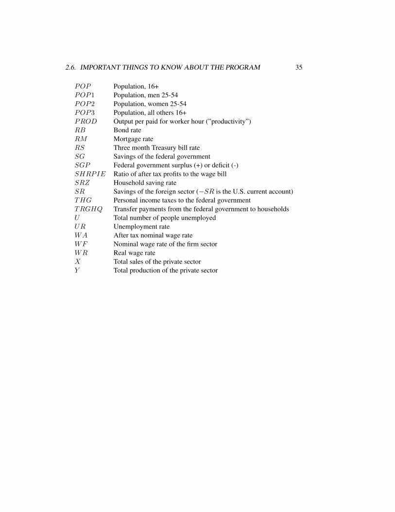
Selecting Variables to Display
The following are some of the variables you might want to display when examiningthe output. This list is a subset of all the variables in the model.

34 CHAPTER 2. A REVIEW OF THE US MODEL
AA Total net wealth of the household sectorAG Net financial assets of the federal government
(-AG is roughly the federal government debt)BO Bank borrowing from the FedBR Total bank reservesCD Consumer expenditures for durablesCG Capital gains (+) or losses (-) on stocks held by householdsCN Consumer expenditures for nondurablesCOG Federal government purchases of goodsCOS State and Local government purchases of goodsCS Consumer expenditures for servicesCUR Currency held outside banksD1G Personal income tax parameter for federal taxesE Total employmentEX ExportsGDPD GDP price deflatorGDPR Real GDPIHH Residential investment, household sectorIKF Nonresidential fixed investment of the firm sectorIM ImportsINTF Interest payments of the firm sectorINTG Interest payments of the federal governmentIV F Inventory investment of the firm sectorJF Number of jobs in the firm sectorKK Capital stock of the firm sectorL1 Labor force, men 25-54L2 Labor force, women 25-54L3 Labor force, all others 16+LM Number of moonlightersMB Net demand deposits and currency of banksMF Demand deposits and currency of the firm sectorMH Demand deposits and currency of the household sectorM1 Money supplyPCGDPD Percentage change in the GDP price deflator (annual rate)PCGDPR Percentage change in real GDP (annual rate)PCM1 Percentage change in the money supply (annual rate)PF Price deflator for the firm sectorPG Price deflator for COGPIEF Before tax profits of the firm sectorPIM Import price deflator
2.6. IMPORTANT THINGS TO KNOW ABOUT THE PROGRAM 35
POP Population, 16+POP1 Population, men 25-54POP2 Population, women 25-54POP3 Population, all others 16+PROD Output per paid for worker hour (”productivity”)RB Bond rateRM Mortgage rateRS Three month Treasury bill rateSG Savings of the federal governmentSGP Federal government surplus (+) or deficit (-)SHRPIE Ratio of after tax profits to the wage billSRZ Household saving rateSR Savings of the foreign sector (−SR is the U.S. current account)THG Personal income taxes to the federal governmentTRGHQ Transfer payments from the federal government to householdsU Total number of people unemployedUR Unemployment rateWA After tax nominal wage rateWF Nominal wage rate of the firm sectorWR Real wage rateX Total sales of the private sectorY Total production of the private sector

36 CHAPTER 2. A REVIEW OF THE US MODEL

Chapter 3
Historical Data
Before running any experiments, it will be useful simply to examine some of themacroeconomic data to see what they look like. Graphs are a good way of getting a“feel” for the data. Since 1970 there are five periods that can be classified as generalrecessionary periods: 1974:1-1975:4, 1980:2-1983:1, 1990:3-1991:1, 2001.1-2001.3,and 2008:1-2009:2. Similarly, two subperiods can be classified as general inflationaryperiods: 1973:2-1975:1 and 1978:2-1981:1. These subperiods are useful for referencepurposes.
In this chapter you are asked to table and graph the variables listed in Section 2.6for the period since 1970:1 and examine how they behave during the recessionary andinflationary subperiods. You should save these tables and graphs for future reference.You may also want to table and graph the variables for the entire period since 1952:1.If you do so, how many other recessionary and inflationary subperiods can you pickout?
In doing the work in this chapter (and the others) you should always use Table A.2in Appendix A as the reference for the variable names. The definition of a variableis not always repeated when the notation for the variable is used in describing theexperiments.————————————————————————————————-
Experiment 3.1: Variables for the 1970:1-2021:1 Period
Table and graph the variables listed in Section 2.6 for the 1970:1-2022141period.Some of the following questions may require more knowledge of macroeconomics
than you currently have. Do your best for now to get a feel for the data, and thencome back to the tables and graphs to review the data from time to time as you gainmore knowledge.
37
38 CHAPTER 3. HISTORICAL DATA
Recessionary Periods
1. From the table and graph for real GDP, GDPR, can you pick out the fourrecessionary periods mentioned above? Which of the other variables tend tofollow the business cycle, and which do not? Can you think of reasons whysome do and some don’t? Focus in particular on the components of GDPRand on the saving rate, SRZ.
Inflationary Periods
1. From the table and graph for the percentage change in the GDP deflator,PCGDPD, can you pick out the two inflationary periods? How does theimport price index, PIM , behave during these periods? How about the nomi-nal wage rate, WA, and the real wage rate, WR?
2. How much overlap is there between the recessionary and inflationary periods?(These overlap periods are called periods of ”stagflation.”) Can you speculateon what might have caused the stagflation? Can you pick out any variables thatyou have graphed as possible culprits?
Labor Market Variables
1. How did the unemployment rate, UR, behave during the recessionary andinflationary periods?
2. Is there a tight relationship between UR and the rate of inflation, PCGDPD?
3. How did productivity, PROD, behave during the recessionary periods? Whymight PROD be procyclical?
4. Calculate the values of the labor force participation rates L1/POP1,L2/POP2, and L3/POP3 for a few of the quarters within the overall pe-riod. Note how they have changed over time, and note the remarkable rise inL2/POP2, the participation rate for women 25-54, since 1970. What mighthave caused this rise?
5. Are the labor force participation rates procyclical or countercyclical or neither?Do they seem to vary with UR? Why might they vary with UR?
Fiscal Policy Variables and Other Federal Government Variables
1. Examine how the fiscal policy variablesCOG,D1G,D2G,D3G,D4G,D5G,and TRGHQ have changed over time.

39
2. Examine how the government deficitSGP and the government debt−AG havechanged over time. What are some of the factors that led to the large rise in thedeficit?
3. Why are interest payments of the government, INTG, growing so rapidly?What consequences does this have for SGP and AG?
Monetary Policy Variables and Other Financial Variables
1. How did the bill rate, RS, behave during the recessionary periods? During theinflationary periods? What does this say about Fed behavior?
2. What is the relationship between the long term bond rate, RB, and RS? Whymight RS fluctuate more than RB?
3. Examine carefully the behavior of RS during the period 1979:4-1982:3. Doesthis behavior seem different than at other times? How did the money supply,M1, behave during this period versus at other times? Does it seem to you thatthe Fed behaved differently during this period than otherwise?
4. Compute velocity, GDP/M1, for a few quarters and examine how it haschanged over time. How stable over time does it seem?
5. What happened to GDPR and GDPD in 1974? What was the monetaryresponse to this in 1975? (Look at RS and M1.)
6. What was the monetary response following the stock market crash in 1987?Can you pick out the effects of the stock market crash on household wealth,AA?
Foreign Sector Variables
1. Examine how PIM , IM , PEX , and EX have changed over time.
2. How has the saving of the foreign sector, SR, changed over time? What arethe main factors that have led to this change? (−SR is roughly the U.S. currentaccount.)
3. SGP and −SR are sometimes call the“twin deficits.” Examine their rela-tionship over time. Can you think of reasons why the two deficits might bepositively correlated?

40 CHAPTER 3. HISTORICAL DATA
Extra Credit
1. If you have tabled or graphed the variables from 1952:1 on, answer the relevantquestions above for this longer period. For example, how many recessions canyou pick out since 1952? How many high inflation periods? Are some of therelationships that were not stable after 1970 closer to being stable before 1970?
————————————————————————————————-

Chapter 4
NIPA and FFA Data
The National Income and Product Accounts (NIPA) and the Flow of Funds Accounts(FFA) are more than just the places where much macroeconomic data come from.They help us organize our thoughts about the structure of the economy, and theyprovide the framework for constructing models of the economy. The exercises in thischapter are designed to get you acquainted with the two sets of accounts.
4.1 Identities
By definition, GDP is equal to consumption plus investment plus government spendingplus exports minus imports. In the US model there are six sectors and a number ofcategories of consumption, investment, and government spending, which make theGDP identity and other identities somewhat more involved. It will be useful to beginwith the definition of total sales of the private sector, denoted X , which is defined inequation 60. Equation 60 is:
X = CS + CN + CD + IHH + IKF + EX − IM + COG+ COS+IKH + IKB + IKG+ IHF + IHB
60
————————————————————————————————-
Experiment 4.1: The Components of X
Table variable X and its components (from equation 60) for 2021:1.
1. Note that some components are quite small. You should use this experimentto get a feel for the size of the various components. Note what a large fractionconsumption is of total sales.
41

42 CHAPTER 4. NIPA AND FFA DATA
————————————————————————————————-By definition production minus sales is the change in inventories. This definition
is equation 63:V = V−1 + Y −X 63
where V is the stock of inventories at the end of the quarter, Y is production, and Xis sales. Also, by definition, the change in inventories is inventory investment, whichis equation 117:
IV F = V − V−1, 117
where IV F is inventory investment. In the model Y is determined by equation 11,which reflects production smoothing behavior, X is determined by the identity 60, Vis determined by the identity 63, and IV F is determined by the identity 117.
Y is not total GDP; it is only the part of GDP produced by the private sector.Some production also takes place in the and government sectors. Equation 83 definesreal GDP as production in the private and government sectors:
GDPR = Y + PSI13 ∗ (JG ∗HG+ JM ∗HM + JS ∗HS) + STATP, 83
the term after Y is production in the federal and state and local government sectors.STATP is a statistical discrepancy pertaining to the use of the chain weighted data,which is discussed in Macroeconometric Modeling.————————————————————————————————-
Experiment 4.2: Going from X to GDPR
Table X , Y , IV F , and GDPR for 2021:1.
1. Note that IV F is small relative to Y and that most of GDPR is Y (i.e., mostof GDPR is produced by the private sector).
————————————————————————————————-
4.2 Nominal versus Real GDP
As any introductory economics textbook discusses, it is important to distinguish be-tween nominal and real GDP. By definition, nominal GDP is equal to real GDP timesthe GDP price index. In the model, this relationship is equation 84, which is used todetermine the GDP price index:
GDPD = GDP/GDPR, 84
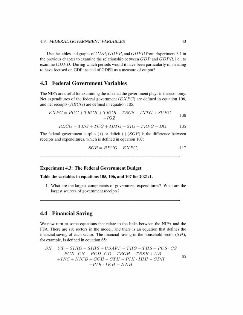
4.3. FEDERAL GOVERNMENT VARIABLES 43
Use the tables and graphs ofGDP ,GDPR, andGDPD from Experiment 3.1 inthe previous chapter to examine the relationship between GDP and GDPR, i.e., toexamine GDPD. During which periods would it have been particularly misleadingto have focused on GDP instead of GDPR as a measure of output?
4.3 Federal Government Variables
The NIPA are useful for examining the role that the government plays in the economy.Net expenditures of the federal government (EXPG) are defined in equation 106,and net receipts (RECG) are defined in equation 105:
EXPG = PUG+ TRGH + TRGR+ TRGS + INTG+ SUBG−IGZ, 106
RECG = THG+ TCG+ IBTG+ SIG+ TRFG−DG, 105
The federal government surplus (+) or deficit (-) (SGP ) is the difference betweenreceipts and expenditures, which is defined in equation 107:
SGP = RECG− EXPG, 117
————————————————————————————————-
Experiment 4.3: The Federal Government Budget
Table the variables in equations 105, 106, and 107 for 2021:1.
1. What are the largest components of government expenditures? What are thelargest sources of government receipts?
————————————————————————————————-
4.4 Financial Saving
We now turn to some equations that relate to the links between the NIPA and theFFA. There are six sectors in the model, and there is an equation that defines thefinancial saving of each sector. The financial saving of the household sector (SH),for example, is defined in equation 65:
SH = Y T − SIHG− SIHS + USAFF − THG− THS − PCS · CS−PCN · CN − PCD · CD + TRGH + TRSH + UB
+INS +NICD + CCH − CTH − PIH · IHH − CDH−PIK · IKH −NNH
65
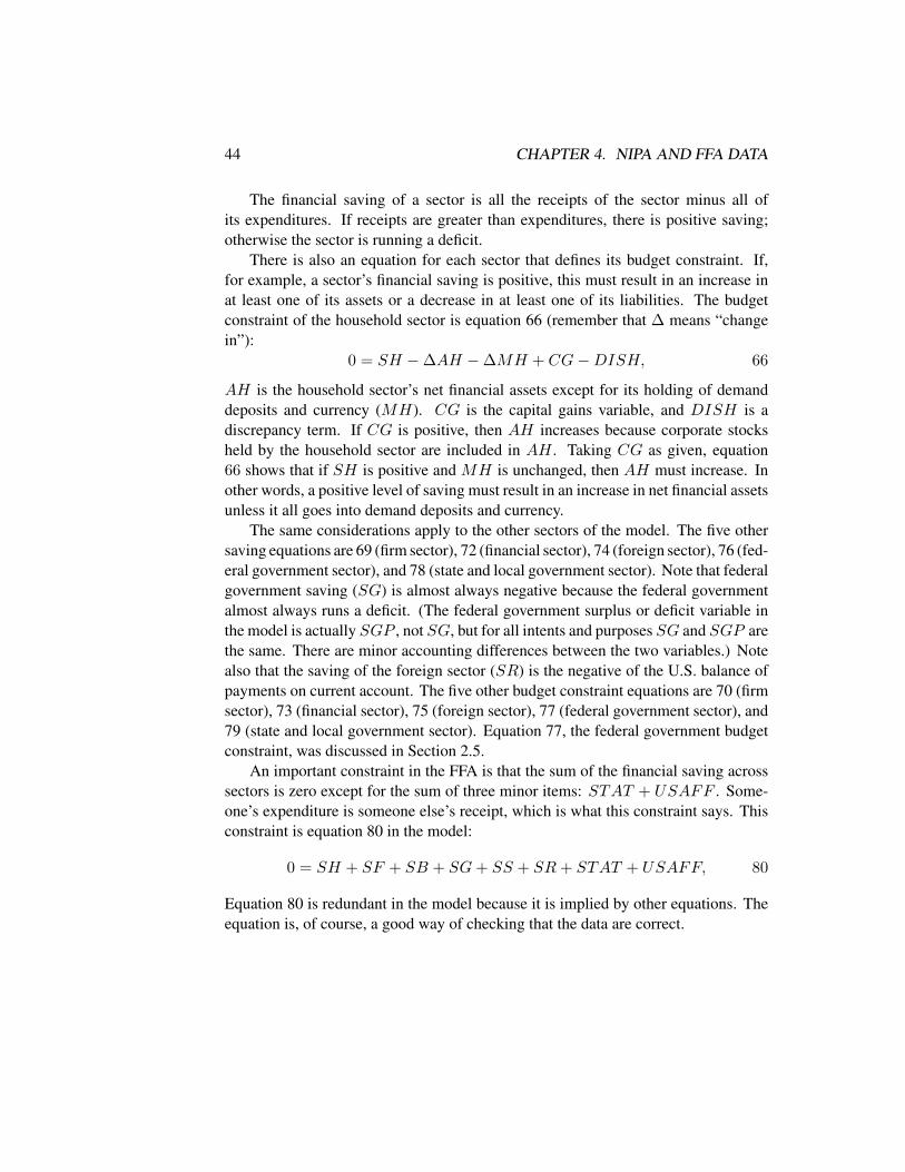
44 CHAPTER 4. NIPA AND FFA DATA
The financial saving of a sector is all the receipts of the sector minus all ofits expenditures. If receipts are greater than expenditures, there is positive saving;otherwise the sector is running a deficit.
There is also an equation for each sector that defines its budget constraint. If,for example, a sector’s financial saving is positive, this must result in an increase inat least one of its assets or a decrease in at least one of its liabilities. The budgetconstraint of the household sector is equation 66 (remember that ∆ means “changein”):
0 = SH − ∆AH − ∆MH + CG−DISH, 66
AH is the household sector’s net financial assets except for its holding of demanddeposits and currency (MH). CG is the capital gains variable, and DISH is adiscrepancy term. If CG is positive, then AH increases because corporate stocksheld by the household sector are included in AH . Taking CG as given, equation66 shows that if SH is positive and MH is unchanged, then AH must increase. Inother words, a positive level of saving must result in an increase in net financial assetsunless it all goes into demand deposits and currency.
The same considerations apply to the other sectors of the model. The five othersaving equations are 69 (firm sector), 72 (financial sector), 74 (foreign sector), 76 (fed-eral government sector), and 78 (state and local government sector). Note that federalgovernment saving (SG) is almost always negative because the federal governmentalmost always runs a deficit. (The federal government surplus or deficit variable inthe model is actually SGP , not SG, but for all intents and purposes SG and SGP arethe same. There are minor accounting differences between the two variables.) Notealso that the saving of the foreign sector (SR) is the negative of the U.S. balance ofpayments on current account. The five other budget constraint equations are 70 (firmsector), 73 (financial sector), 75 (foreign sector), 77 (federal government sector), and79 (state and local government sector). Equation 77, the federal government budgetconstraint, was discussed in Section 2.5.
An important constraint in the FFA is that the sum of the financial saving acrosssectors is zero except for the sum of three minor items: STAT + USAFF . Some-one’s expenditure is someone else’s receipt, which is what this constraint says. Thisconstraint is equation 80 in the model:
0 = SH + SF + SB + SG+ SS + SR+ STAT + USAFF, 80
Equation 80 is redundant in the model because it is implied by other equations. Theequation is, of course, a good way of checking that the data are correct.

4.4. FINANCIAL SAVING 45
————————————————————————————————-
Experiment 4.4: Saving Equations and Budget Constraints
Table the variables in equations 65 and 66 for 2020:4 and 2021:1. Do the samefor the variables in equations 69 and 70, in equations 72 and 73, in equations 74and 75, in equations 76 and 77, and in equations 78 and 79.
1. Note that the budget constraints are met in the data aside from rounding errors.
2. Observe that the six saving variables, SH , SF , SB, SG, SS, and SR, sum to−STAT − USAFF . Who are the big savers and who are the big dissavers?
3. Check equation 77 carefully, and review the discussion of this equation inSection 2.5.
4. Check the budget constraint for the foreign sector carefully. Why hasAR beenincreasing so rapidly recently?
————————————————————————————————-The final constraint that will be discussed is the demand deposit identity, equa-
tion 71:
0 = ∆MB + ∆MH + ∆MF + ∆MR+ ∆MG+ ∆MS − ∆CUR, 71
MH , MF , MR, MG, and MS are demand deposit and currency holdings of thevarious sectors. CUR is the amount of currency in the hands of the public. MB isthe total amount of demand deposits held; it is negative because demand deposits area liability of banks.————————————————————————————————-
Experiment 4.5: The Demand Deposit Identity
Table the variables in equation 71 for 2020:4 and 2021:1.
1. Check that equation 71 is met for 2021:1. Which sector holds the largest amountof demand deposits and currency? Which sector holds the smallest?
————————————————————————————————-

46 CHAPTER 4. NIPA AND FFA DATA

Chapter 5
Fiscal Policy Effects underAlternative Assumptions aboutMonetary Policy
A good way to learn about the properties of a model (and if the model is any goodabout the properties of the economy) is to consider the effects of changing variousfiscal policy variables. We know from Chapter 2 that fiscal policy effects dependon what is assumed about monetary policy, and so we must also consider monetarypolicy in this chapter. We begin with a very straightforward experiment: a decrease ingovernment purchases of goods with the interest rate reaction function used. Federalgovernment purchases of goods in the model is denoted COG. COG is to be decreasedwith equation 30 used.
5.1 Changes in Government Purchases of Goods
————————————————————————————————-
Experiment 5.1: Increase in Government Spending, Interest Rate Reac-tion Function
Change COG by 10 in each quarter of the forecast period. The default optionin the program is to use the interest rate reaction function (equation 30), and sono changes are needed regarding the assumption about monetary policy. Solvethe model.
47

48 CHAPTER 5. FISCAL POLICY EFFECTS
The following are some of the questions you should consider about this exper-iment, but they are by no means exhaustive. You should add to the list. For mostquestions, you should focus on the results about four quarters out. After four quartersthe economy has adjusted enough to the government spending change for the effectsto be noticeable.
1. How are the following variables affected over time and why: real GDP(GDPR), the price level (PF ), the unemployment rate (UR), the short terminterest rate (RS), and the federal government deficit (SGP )? Note that thechange in GDPR divided by the change in COG is the multiplier. How doesthe multiplier change over time? Why?
2. Examine how the main components of GDP are affected and try to explain whythey move the way they do: CS, CN , CD, IHH , IKF , IV F , and IM .
3. Note that in the first quarter of the change the increase in X is greater than theincrease in Y . Why? Relate this to the theory behind equation 11.
4. Examine the employment and labor force responses in the model, and again tryto explain the reasons behind the movements: JF , E, L1, L2, L3, and LM .What happened to productivity, PROD?
5. Why did RS increase? Why did RB and RM increase? What happened toM1 and why?
6. What happened to the change in stock prices, CG, initially and then over time?Why?
7. How did AG change? (−AG is the value of federal government securitiesoutstanding.) Why?
8. How was the level of profits, PIEF , affected? How was the saving rate of thehousehold sector, SRZ, affected?
9. What happened to the percentage change in the real wage, WR, and why?
10. Use the discussion in Section 2.4 to help you in understanding the reasons forthe results.
————————————————————————————————-

5.2. OTHER FISCAL POLICY VARIABLES 49
The second experiment is the same as the first except that the interest rate, RS, istaken to be exogenous.————————————————————————————————-
Experiment 5.2: Increase in Government Spending, Interest Rate Un-changed
Change COG by 10 in each quarter of the forecast period. Take RS to beexogenous. Solve the model.
1. The key feature of this experiment is that it is more expansionary than Experi-ment 5.1. Explain carefully why.
2. How did the Fed’s behavior differ in this experiment from that in the first one?In which experiment was the change in AG larger in absolute value? Why?
————————————————————————————————-The experiments so far have been for a permanent change in government purchases
of goods. The next experiment examines the effects of a temporary change. Thisexperiment is the same as Experiment 5.1 except that the change in COG is only forthe first quarter.————————————————————————————————-
Experiment 5.3: Temporary Increase in Government Spending, InterestRate Reaction Function
Change COG by 10 in the first quarter of the forecast period. Use the interestrate reaction function—the default. Solve the model.
1. Compare the results of this experiment with those of Experiment 5.1. (Notethat the results for the first quarter are the same.)
2. How long does it take for the effects of the COG change on the economy to beessentially negligible?
————————————————————————————————-
5.2 Other Fiscal Policy Variables
We now turn to other tools of fiscal policy. For the rest of the experiments in this chap-ter we will use the interest rate reaction function as our assumption about monetary

50 CHAPTER 5. FISCAL POLICY EFFECTS
policy. Keep in mind, however, that somewhat different results would be obtained ifinstead we took RS to be exogenous.
Say that instead of increasing government spending COG by $10 billion, youwanted to lower personal income taxes by approximately the equivalent amount.How do you do this? The federal personal income tax rate in the model is D1G, andso D1G needs to be lowered. Say that we want D1G to be lowered so that the initialimpact of the tax decrease adds about the same amount money to the economy as didthe increase in COG. COG is in real terms and tax payments are in nominal terms,and so the first thing we need to do is to convert the $10 billion increase in COGinto nominal terms. PG in the model is the price index for COG, and its value in2021:1 was 1.105. The nominal change in government spending corresponding to a$10 billion real change is thus $10 billion times 1.105 = about $11 billion. We thusneed to lower taxes by $11 billion.
The level of federal personal income taxes in the model (THG) is determined byequation 47:
THG = [D1G+ (TAUG · Y T )/POP ]Y T, 47
where Y T is taxable income. The federal tax system is estimated in the model tobe slightly progressive, and so the tax rate increases as Y T increases. TAUG is theestimated progressivity parameter. Now, the question is, in order to decrease THGby $11 billion, how much do we have to lower D1G? To answer this, we need toknow the level of Y T . Y T in 2021:1 was $4,091.5 billion, and $11 billion is .269percent of this. Therefore, we need to lower D1G by .00269. We will so this in thefollowing experiment.
You should be aware that calculations like we have just done are rough. You cannotchange D1G to hit a particular change in THG exactly because Y T is endogenous.As D1G is changed, the economy changes, including Y T , and so THG will alsochange for this reason as well as from the initial change in D1G. Calculations likethe above give one a fairly good idea where to start, but it may be after the first runthat you want to adjust D1G slightly to meet more accurately the THG target.————————————————————————————————-
Experiment 5.4: Decrease in the Personal Income Tax Rate, Interest RateReaction Function
ChangeD1G by -.00269 in each quarter of the forecast period. Solve the model.
1. Compare the results of this experiment with those of Experiment 5.1. Why isthe economy slower to respond in this case? Which policy change is best fordecreasing the federal government deficit and why?

5.2. OTHER FISCAL POLICY VARIABLES 51
2. What does the Fed do in response to the decrease in taxes and why?
3. How has the tax rate decrease affected the labor force? How has it affected thepersonal saving rate, SRZ?
————————————————————————————————-Another important fiscal policy variable is TRGHQ, the level of transfer pay-
ments from the federal government to households. TRGHQ is in real terms. Say thatinstead of decreasing the personal tax rate to lower personal taxes by approximately$11 billion in real terms, the government wanted to increase TRGHQ by $11 billion.The experiment is:————————————————————————————————-
Experiment 5.5: Increase in Transfer Payments, Interest Rate ReactionFunction
Change TRGHQ by 11 in each quarter of the forecast period. Solve model.
1. Compare the results of this experiment to those of Experiments 5.1.
2. Compare the different labor force responses between this experiment and Ex-periment 5.1. How do these differences affect the unemployment rate? Inanswering this question, review the discussion in Section 2.4 under the heading”Labor Supply and the Unemployment Rate.”
3. Although the model has nothing to say about this, are the distributional con-sequences of lowering D1G versus raising TRGHQ likely to be different?How?
————————————————————————————————-There are other fiscal policy variables that can be changed, which you may want
to do as additional assignments. The following are additional changes that can bemade.
Changes in the Profit Tax Rate D2G
WARNING: Please read Section 2.4 under the heading“Tax Rate Effects” regardingthe likely effects of changing D2G. Changing D2G may not be a sensible thing todo.
Federal corporate profit taxes (TFG) is determined in equation 49:
TFG = D2G(PIEF − TFS), 49
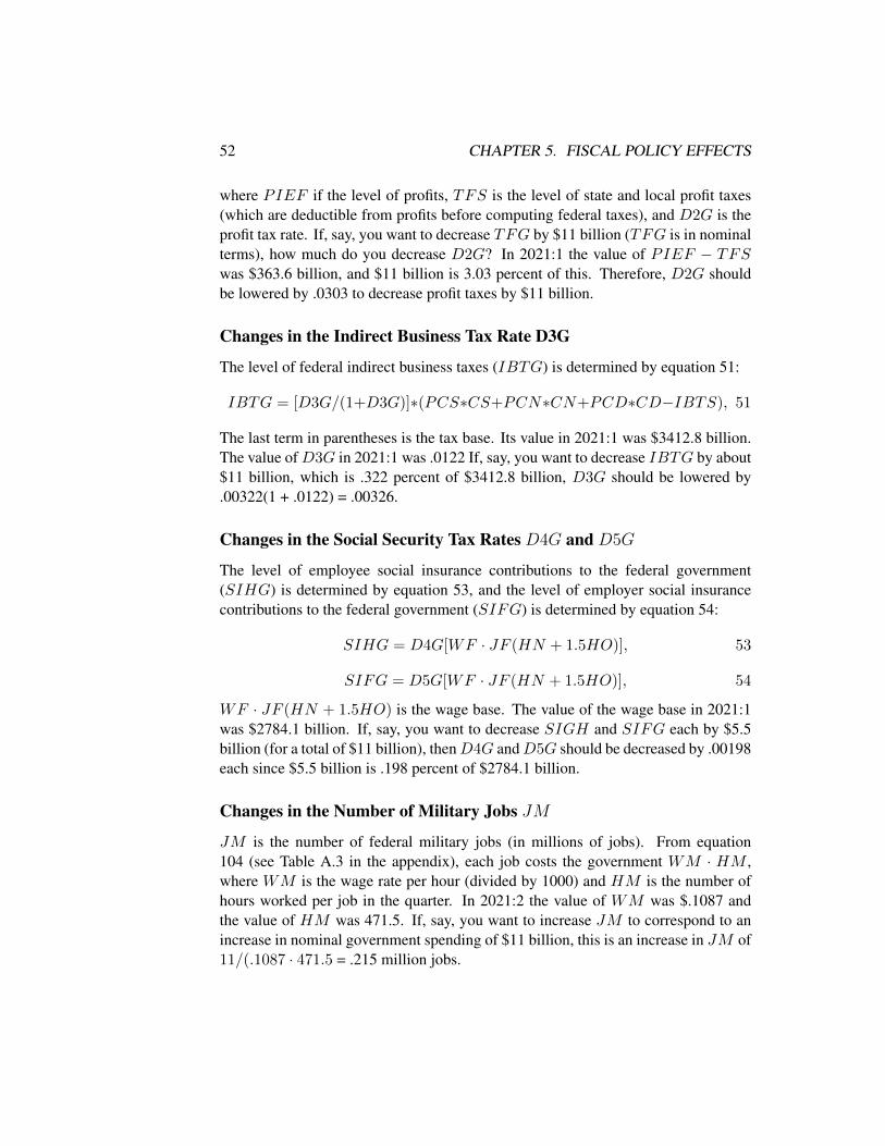
52 CHAPTER 5. FISCAL POLICY EFFECTS
where PIEF if the level of profits, TFS is the level of state and local profit taxes(which are deductible from profits before computing federal taxes), and D2G is theprofit tax rate. If, say, you want to decrease TFG by $11 billion (TFG is in nominalterms), how much do you decrease D2G? In 2021:1 the value of PIEF − TFSwas $363.6 billion, and $11 billion is 3.03 percent of this. Therefore, D2G shouldbe lowered by .0303 to decrease profit taxes by $11 billion.
Changes in the Indirect Business Tax Rate D3G
The level of federal indirect business taxes (IBTG) is determined by equation 51:
IBTG = [D3G/(1+D3G)]∗(PCS∗CS+PCN∗CN+PCD∗CD−IBTS), 51
The last term in parentheses is the tax base. Its value in 2021:1 was $3412.8 billion.The value ofD3G in 2021:1 was .0122 If, say, you want to decrease IBTG by about$11 billion, which is .322 percent of $3412.8 billion, D3G should be lowered by.00322(1 + .0122) = .00326.
Changes in the Social Security Tax Rates D4G and D5G
The level of employee social insurance contributions to the federal government(SIHG) is determined by equation 53, and the level of employer social insurancecontributions to the federal government (SIFG) is determined by equation 54:
SIHG = D4G[WF · JF (HN + 1.5HO)], 53
SIFG = D5G[WF · JF (HN + 1.5HO)], 54
WF · JF (HN + 1.5HO) is the wage base. The value of the wage base in 2021:1was $2784.1 billion. If, say, you want to decrease SIGH and SIFG each by $5.5billion (for a total of $11 billion), thenD4G andD5G should be decreased by .00198each since $5.5 billion is .198 percent of $2784.1 billion.
Changes in the Number of Military Jobs JM
JM is the number of federal military jobs (in millions of jobs). From equation104 (see Table A.3 in the appendix), each job costs the government WM · HM ,where WM is the wage rate per hour (divided by 1000) and HM is the number ofhours worked per job in the quarter. In 2021:2 the value of WM was $.1087 andthe value of HM was 471.5. If, say, you want to increase JM to correspond to anincrease in nominal government spending of $11 billion, this is an increase in JM of11/(.1087 · 471.5 = .215 million jobs.

5.2. OTHER FISCAL POLICY VARIABLES 53
Changes in the Number of Federal Government Civilian Jobs JG
Similar considerations apply to the number of civilian jobs JG. From equation 104,the cost of a civilian job to the government is WG ·HG, where WG is the wage rateper hour (divided by 1000) and HG is the number of hours worked per job in thequarter. In 2021:1 the value ofWGwas $.0468 and the value ofHGwas 499.1. If youwant to increase JG to correspond to an increase in nominal government spendingof $11 billion, this is an increase in JG of 11/(.0468 ∗ 499.1) = 0.471 million jobs.
Change in Grants in Aid to State and Local Governments TRGSQ
TRGSQ is the level of grants in aid to state and local governments from the federalgovernment. It is in real terms, and you can change it like TRGHQ was changedin Experiment 5.5. Remember, however, that any change in TRGSQ is likely tochange state and local government behavior. If you increase TRGSQ, state and localgovernments are likely to spend more or tax less, and if you decrease TRGSQ, theyare likely to spend less or tax more. You should thus change some state and localgovernment variable along with TRGSQ in order for the experiment to be sensible.
A Note on Being Sensible
You should be aware that large, rapid changes in government policy variables are notrealistic. It takes time for the government to put policy changes into effect, and thepolitical process is such that large changes are seldom done. Also, if you make largechanges in policy variables, the results from the model are less trustworthy than ifyou make small changes. Changes in policy variable that are outside the range of pastchanges means that you are analyzing events that are historically unprecedented, andsince models are estimated over historical data, they may not capture the effects ofextreme events well. So don’t go wild with the policy variables.

54 CHAPTER 5. FISCAL POLICY EFFECTS

Chapter 6
Monetary Policy Effects
When the interest rate reaction function—equation 30—is included in the model,monetary policy is endogenous. In other words, there is no exogenous monetarypolicy variable to change. One can, however, drop equation 30 and examine theeffects of exogenous changes in RS. This is done in experiment 6.1.————————————————————————————————-
Experiment 6.1: Increase in the Short Term Interest Rate RS
Take RS to be exogenous and increase it by 1.0 in each quarter of the forecastperiod. Solve the model.
1. Answer the questions posed at the end of Experiment 5.1. (Experiment 6.1 isanother key experiment that you should have a good understanding of.)
2. What did M1 do in response to the increase in RS? Why?
3. Remember that −AG is the value of government securities outstanding. Thisis the open market operations variable of the Fed. Note that −AG increased inthe experiment. Why?
4. What was the effect on government interest payments INTG? How did thisaffect SGP ?
————————————————————————————————-
55

56 CHAPTER 6. MONETARY POLICY EFFECTS

Chapter 7
Price Shocks and Stock MarketShocks
7.1 Price Shocks
The key exogenous variable regarding the behavior of prices is the price of imports(PIM ). If PIM increases, this increases domestic prices through the price equa-tion 10. The effect of a change in PIM on domestic prices is in fact quite large.Experiment 7.1 examines this question.————————————————————————————————-
Experiment 7.1: Increase in the Import Price Index PIM
Increase PIM by 10 percent in each quarter of the forecast period. Solve themodel.
1. Note that stagflation resulted from this experiment. Why? In particular, whydid aggregate expenditures fall in real terms?
2. What did the Fed do in response to all of this? (Remember that equation 30 isin the model for this experiment since it is the default option and you made nochanges regarding monetary policy.)
3. What happened to the real wage and why? To the labor force? To the householdsaving rate? To corporate profits in nominal terms (PIEF )? To corporateprofits in real terms (PIEF/PF )?
————————————————————————————————-
57
58 CHAPTER 7. PRICE SHOCKS AND STOCK MARKET SHOCKS
The model attributes much of the stagflation of the 1970’s to the huge increase inPIM that occurred during this period. This can be seen in the following experiment.————————————————————————————————-
Experiment 7.2: What if PIM had not changed after 1973?
Set the prediction period to be 1974:1–1978:4. Ask to use the historical errors.Change the values of PIM for 1974:1-1978:4 to be equal to the actual value in1973:4. Solve the model.
1. How different would the U.S. economy have been had PIM not changed fromits value in 1973:4, i.e., had there been no oil price shock? Examine the keyvariables in the model. How much of the stagflation during this period does themodel attribute to PIM?
2. What does the model estimate the Fed would have done differently had PIMnot risen? How would AG have been different?
3. How would the labor force have been different, and what would the unemploy-ment rate have been?
4. This is an important experiment in that it shows that according to the modelthe 1970’s would have been fine had it not been for the oil shock and the otherprice shocks that caused PIM to increase so rapidly.
————————————————————————————————-

7.2. STOCK MARKET SHOCKS 59
7.2 Stock Market Shocks
Almost everyone knows the stock market crashed in October of 1987. After the crash,how was the economy affected? The model can be used to estimate these effects. Thestock market variable in the model is CG, the capital gains (+) or losses (-) on stocksheld by the household sector. The crash in October resulted in a fall in CG of about$500 billion. Although the October crash is history, we can ask how the economywould respond if there were a large fall in, say, 2021:2, the first quarter of the forecastperiod. We will assume a fall of $2000 billion in 2021:2, but no further fall after that.————————————————————————————————-
Experiment 7.3: Stock Market Crash in 2021:2
Drop equation 25, and change the value of CG in 2021:2 by -2000. Solve themodel for the forecast period (beginning in 2021:2
1. How did the crash affect household net wealth, AA? How did householdsrespond to this change in AA regarding consumption and labor supply? (Notethat there is a lag of one quarter in the effects of AA on household behavior.)
2. What roughly was the fall in consumption per year as a percent of the fall inAA? Does this percent seem reasonable?
3. How did the Fed respond to the crash?
4. What is roughly the loss of real GNP per year as a result of the crash?
5. This experiment is important in that it shows that a crash of this size may resultin a recession, but not a depression.
————————————————————————————————-

60 CHAPTER 7. PRICE SHOCKS AND STOCK MARKET SHOCKS

Chapter 8
Housing Price Shocks
Nominal housing wealth in the model is PKH ·KH , where KH is the real stock ofhousing and PKH is the market price ofKH . Nominal housing wealth enters in thedefinition ofAA (equation 89), which is the wealth variable that affects consumptiondemand (equations 1, 2, and 3). PKH is determined (equation 55) as PSI14 · PD,where PD is the price deflator for domestic sales and PSI14 is exogenous. It is thuspossible to change housing wealth in the model by changing PSI14. For example,if you think housing prices are going to fall (relative to PD) in the future, you candecrease PSI14. This is done in the experiment in this chapter. It allows you to seethe estimated effects on the economy of falling housing prices.————————————————————————————————-
Decrease in PSI14
Decrease PSI14 by 20 percent for the forecast period. Solve the model.
1. How much did nominal housing wealth, PKH ·KH , fall? How much did thereal wealth variable AA fall?
2. What effect did this change have on the consumption variables, CS, CN , andCD? On the labor supply variables, L1, L2, L3, and LM? (Note that there isa lag of one quarter in the effects of AA on household behavior.)
3. How did the Fed respond to the fall in housing prices?
4. What is roughly the loss of real GNP per year as a result of the fall in housingprices?
————————————————————————————————-
61

62 CHAPTER 8. HOUSING PRICE SHOCKS

Chapter 9
Sensitivity of the Results to theFed’s Weight on Inflation
Equation 30, the interest rate reaction function, is estimated. It is an estimate of Fedbehavior. The coefficient estimate on inflation in this equation is an estimate of howthe Fed responds to inflation regarding its interest rate policy. The experiment in thischapter asks the question of how much different it would make regarding fiscal-policyeffects if the inflation coefficient were larger.
We have seen in Chapter 5, Experiment 5.1, how the economy responds to anincrease in COG when the interest rate reaction function is used. We now examinethe question of how the results change when the Fed’s weight on inflation is larger. Wewill make the inflation coefficient in equation 30 three times as large as the estimatedvalue and then rerun Experiment 5.1 for this version of the model.————————————————————————————————-
Experiment 9.1: Experiment 5.1 with more weight on inflation in equation30
Triple the third coefficient in equation 30. Solve the model for the forecastperiod. Call this dataset BASEA. Create a new dataset using BASEA as yourbase dataset. Call this dataset NEWA. ChangeCOG by 10 in each quarter of theforecast period. Solve the model for the forecast period. Answer the followingquestions by comparing NEWA to BASEA. (You should use names other thanNEWA and BASEA because these have already been used. It doesn’t matterwhat the dataset names are.)
1. Note that a new base dataset had to be created because a coefficient was changed.The predictions of the new version of the model are not the same as the pre-
63

64 CHAPTER 9. FED’S WEIGHT ON INFLATION
dictions in ZAJBASE, and so a new base dataset had to be created. It is notof interest to compare the predicted values in BASEA with the values in ZA-JBASE. They differ, but only because a coefficient estimate has been arbitrarilychanged. Make sure you understand what is going on here.
2. Compare these results to those of Experiment 5.1. Explain carefully the dif-ferences. Do these differences make sense given that the Fed now cares moreabout inflation?
————————————————————————————————-There are many other experiments of this type that you can perform. For exam-
ple, you can change other coefficients in equation 30, say increasing the weight onunemployment, and examine how this affects the results of changing COG. You canalso run different fiscal-policy experiments (other than just changingCOG) once youhave your new version of the model. Be sure each time you change a coefficient thatyou get a new base dataset (like BASEA above).

Chapter 10
Sensitivity of the Results to theInterest Elasticity of AggregateExpenditures
An important issue in a macroeconomic model is the interest elasticity of aggregateexpenditure. How much do consumption and investment respond to changes in interestrates? How much would the properties of the model change if the responses weredifferent? These questions can be analyzed by running different experiments. Wefirst consider the case in which the interest elasticity of consumer expenditures fordurable goods is larger. We then explore the case in which the interest elasticity ofnonresidential fixed investment equation is larger.————————————————————————————————-
Experiment 10.1: Experiment 6.1 with more Interest Elastic ConsumerExpenditures
Change the eighth coefficient in equation 3 to be twice its size in absolute value.Solve the model for the forecast period. Call this dataset BASEA. Create a newdataset using BASEA as your base dataset. Call this dataset NEWA. TakeRS tobe exogenous, and increaseRS by 1 in each quarter of the forecast period. Solvethe model for the forecast period. Call this dataset NEWA. Answer the followingquestions by comparing NEWA to BASEA. (As mentioned in Experiment 9.1,you should use names other than NEWA and BASEA.)
1. Note that as in Experiment 9.1 a new base dataset had to be created becausea coefficient was changed. The predictions of the new version of the modelare not the same as the predictions in ZAJBASE, and so a new base dataset
65
66CHAPTER 10. INTEREST ELASTICITY OF AGGREGATE EXPENDITURES
had to be created. Again, it is not of interest to compare the predicted valuesin a dataset like BASEA with the values in ZAJBASE. They differ, but onlybecause a coefficient estimate has been arbitrarily changed.
2. Compare these results with those of Experiment 6.1. Explain the differencescarefully.
————————————————————————————————-————————————————————————————————-
Experiment 10.2: Experiment 6.1 with more Interest Elastic CapitalStock
Change the ninth coefficient in equation 12 to be twice its size in absolute value.Solve the model for the forecast period. Call this dataset BASEA. Create a newdataset using BASEA as your base dataset. Call this dataset NEWA. TakeRS tobe exogenous, and increase RS by 1 in each quarter of the forecast period. Solvethe model for the forecast period. Call this dataset NEWA. Answer the followingquestions by comparing NEWA to BASEA. (As mentioned in Experiment 9.1,you should use names other than NEWA and BASEA.)
1. Compare these results with those of Experiment 6.1. Explain the differencescarefully. In particular, how does the behavior of nonresidential fixed invest-ment, IKF , differ? Remember that IKF is equal to the change in the capitalstock plus depreciation (equation 92).
————————————————————————————————-

Chapter 11
Sensitivity of the Results to theSpecification of the Price Equation
Prices in the model respond only modestly to changes in the unemployment rate.This seems to be what the data are telling us, but many may feel that prices arelikely to respond more than the model indicates. It is easy to change the model tomake it more price sensitive to unemployment changes. This is done by making thecoefficient of the unemployment rate in equation 10 larger in absolute value. This iswhat Experiment 11.1 does.————————————————————————————————-
Experiment 11.1: Experiment 5.1 with a more Unemployment SensitivePrice Equation
Change the fifth coefficient in equation 10 to be twice its size in absolute value.Solve the model for the forecast period. Call this dataset BASEA. Create a newdataset using BASEA as your base dataset. Call this dataset NEWA. ChangeCOG by 10 each quarater. Solve the model for the forecast period. Call thisdataset NEWA. Answer the following questions by comparing NEWA to BASEA.(As mentioned in Experiment 9.1, you should use names other than NEWA andBASEA.)
1. The price index PF rises more in this experiment than it does in Experiment5.1. Why? Do you think the price response should be even larger?
2. Why was the increase in real GDP slightly less here than in Experiment 5.1?Be sure to trace through the effects.
3. How did the Fed behave here as compared to Experiment 5.1?
67

68 CHAPTER 11. SPECIFICATION OF THE PRICE EQUATION
————————————————————————————————-The sensitivity of prices to changes in demand is one of the key questions in
macroeconomics, and experiments like 11.1 help to examine it.

Chapter 12
Foreign Sector Effects
The two key exogenous foreign sector variables in the model are the real value of ex-portsEX and the price index for imports PIM . Imports IM and the price of exportsPEX are endogenous. We have seen the effects of changing PIM in Experiments7.1, 7.2, and 8.6. We have seen the effects of changing EX in Experiments 8.4 and8.5.
It is not always sensible to take EX and/or PIM to be exogenous when exper-iments are being run, and we have so far ignored this problem. Without building amulticountry model, it is not really possible to endogenize EX and PIM , but a fewpartial steps in this direction can be taken. Say that you are increasing interest ratesand you feel that this will lead to an appreciation of the dollar. If the dollar appreciates,PIM should go down (imports will be cheaper in dollars) and EX should go down(U.S. exports are now more expensive in foreign currencies). There are, of course,lags in the effects of exchange rate changes on PIM and EX , and these lags can befairly long.
You can take foreign sector effects into account in the model if you are willing tospecify ahead of time how PIM and EX are affected by whatever change you aremaking. You can enter your changes to PIM andEX along with your other changesand then solve the model. In the example of an interest rate increase, you will haveto specify 1) how the interest rate increase affects the value of the dollar, 2) how thechange in the value of the dollar translates into a change in PIM , and 3) how thechange in the value of the dollar translates into a change in the U.S. price of exportsin foreign currencies and how this in turn affects EX .
There is obviously some work involved in doing this, but it is necessary to dothis short of constructing a complete multicountry model. Fortunately, there are onlytwo key variables that you need worry about, PIM and EX , and so the adjustmentsare not too burdensome. Also, many of the changes that one makes when running
69

70 CHAPTER 12. FOREIGN SECTOR EFFECTS
experiments are likely to have only minor effects on PIM and EX , and so in manycases ignoring these effects is not likely to be very serious.

Chapter 13
Other Possible Experiments
The suggested experiments in this workbook by no means exhaust the possible exper-iments that can be performed. Indeed, the workbook is really only meant to get youstarted on your way to your own analysis of macroeconomic questions and issues.This chapter presents a few more possible experiments for you to ponder.
13.1 Combinations of Policies
It is best when first learning about the properties of a model to change only oneexogenous variable at a time. Otherwise, one can get hopelessly lost in trying tofigure out what is affecting what. In practice, however, one is usually concerned withmore than one exogenous variable at a time. The government may want to knowthe consequences of changing both taxes and government expenditures at the sametime. A business forecaster may want to know the outcome of an increase in importprices and an increase in exports. You would probably want to change state and localgovernment expenditures or taxes at the same time that you change federal grants inaid to state and local governments.
Now that you have gone through the workbook, you should not be shy about tryingmore complex sets of exogenous variable changes. If you know the consequences ofchanging one variable at a time, you should be able to explain the outcome when manyvariables are changed. A common type of experiment to perform is to pick a target pathfor some endogenous variable, say the federal government deficit, and keep changingpolicy variables until the target path is roughly met. You can answer questions likethe following. What combinations of monetary and fiscal policy changes would leadto the target path being met, and are any of these combinations politically feasible?The variety of these types of experiments is quite large. Note also that you can phasein changes in policy variables. It is not necessary, for example, to have COG change
71
72 CHAPTER 13. OTHER POSSIBLE EXPERIMENTS
by $10 billion from the first quarter on or to haveRS change by one percentage pointbeginning immediately. The changes can differ by quarters and gradually work up tothe final change that is desired.
Don’t forget that any experiment that you choose can be performed with differentversions of the model. The types of changes in the model that were made in Chapters9-11 can be made for any experiment.
13.2 Effects of Changing State and Local Government Vari-ables
The tax and spending variables of the state and local government sector are similarto those of the federal government sector. These variables are changed in the sameway that federal government variables are changed. The same types of experimentsthat were performed in Chapter 5 for the federal government can be performed forthe state and local governments.
13.3 Imposing Rational Expectations on the Model
In some cases it is possible to impose rational expectations on the model. Considerthe bond market and the bond rate RB. RB is determined in the model by the termstructure equation 23, where RB is a function of current and lagged values of theshort term interest rateRS. If there are rational expectations in the bond market, thenRB should instead be a function of current and expected future values of RS, wherethe expected future values of RS are what the model predicts them to be.
Say we take an seven quarter horizon and we take RB to the be average of RSand the next six future values of RS:
RB = (1/7)(RS +RS+1 +RS+2 +RS+3 +RS+4 +RS+5 +RS+6)
where the future values of RS are those predicted by the model. Can this version ofthe model be analyzed using the program. The answer is yes, with a little extra work.The way this is done is as follows.
1. Specify the above equation for RB and the same equation for RM . Dropequations 23 and 24.
2. Pick a prediction period, say 2021:2-2023:1. Choose eight future values ofRSfor the eight quarter period beyond the end of the prediction period (i.e., for theperiod 2023:2-2025:1). These eight values will remain the same throughout

13.3. IMPOSING RATIONAL EXPECTATIONS ON THE MODEL 73
the analysis they are your guesses as to what the RS values will be in theseeight quarters.
3. Given your guessed values and the base values of RS, compute RB from theabove equation for each quarter of the prediction period (2021:2-2023:1). Dothe same for RM . (If the RM equation is the same as the RB equation, thenRM is always equal to RB.) Enter these values of RB and RM into theprogram (you can do this because equations 23 and 24 are dropped and thusRB and RM are exogenous).
4. Solve the model for the 2021:2-2023:1 period (making no other changes). Thenew solution values ofRS will in general be different from the base values youused to compute RB and RM . Now use these new values of RS to computenew values of RB and RM and enter the new values of RB and RM into theprogram. Solve the model again. Use the new values of RS to compute newvalues of RB andRM , enter the new values of RB andRM , and solve again.Keep doing this until the new solution values ofRS are close to the values fromthe previous solution. At this point you have converged. The values ofRB andRM are consistent with the future values of RS, and expectations in the bondand mortgage market can be said to be rational. Convergence c an usually beachieved to a reasonable level of accuracy in less than 10 iterations.
5. You are not really done at this point, however, because presumably you wouldlike to use this new version of the model to analyze policy changes. Call the lastdataset you created in step 4 (the dataset for which convergence was achieved)BASER. This is your base dataset for the new version of the model. Now takeBASER as your base dataset and make a policy change, such as a change inCOG. Solve the model, and call the new dataset NEWA. (Remember thatthe use of BASER as the base dataset means that RB and RM are treated asexogenous.) NEWA is not, however, the final dataset to compare to BASERbecause the predicted values ofRS in NEWA are not consistent with the valuesof RB and RM that are in the dataset. You must now change the values ofRB and RM (using the above equation) to be consistent with the new valuesof RS. Enter these in the program and solve again. Keep doing this until youreach convergence. Call the dataset at the point of convergence NEWR.
6. You can now compare the solution values in NEWR with those in BASER.These differences are the effects of the policy change in the new version ofthe model, the version in which there are rational expectations in the bond andmortgage markets.

74 CHAPTER 13. OTHER POSSIBLE EXPERIMENTS
If you work through and understand this example, you can probably think of otherways of adding rational expectations to the model. Iteration in the above manner isfairly straightforward and not too much extra work once you get practiced.
13.4 Making Major Changes to the Model
The site is limited in how much you can change the model. You can drop equationsand change coefficients. You cannot, however, add variables to the equations, andyou cannot add new equations (except ones that have been dropped previously). For-tunately, there is software that allows you to change the model as much as you want.If you use the US model in the Fair-Parke program, you can respecify the existingequations, add new equations, reestimate, and then solve the new version. In fact,if you don’t like anything in the US model except the identities (which no one cancomplain about since they are always true), you can start from scratch and specifyyour own stochastic equations. Once you get your version of the model specifiedand estimated, you can use the Fair-Parke program to change policy variables andexamine the model’s properties. The range of possibilities here is essentially endless.
13.5 Supply Side Experiments
Some“supply side” experiments are not sensible to perform within the model. Themain example concerns the variableLAM in equation 94. If, say, you increaseLAM ,this makes labor more productive. If labor is suddenly more productive, there is moreexcess labor on hand, which has a negative effect on employment demand and hourspaid for (JF and HF ). These are not likely to be the effects one has in mind whenconsidering exogenous productivity increases. There is simply no direct way in whichproductivity increases stimulate demand in the model, and if this is what one has inmind, the model is of really no use for this purpose. Supply experiments like priceshocks are fine to run, but you should probably stay away from changing LAM.
Regarding supply side experiments, note that changing variables like tax rates thataffect the labor force have supply side components. If personal tax rates are lowered,more people enter the labor force looking for work (the quantity of labor suppliedincreases). This in and of itself, however, does not create new jobs, only more peoplelooking for jobs. Unless something is done to create new jobs, the main thing thathappens when the labor force increases is that the unemployment rate increases. (Atax cut, of course, also stimulates demand, and so in this example new jobs will becreated.)

13.6. COUNTERFACTUAL EXPERIMENTS 75
13.6 Counterfactual Experiments
It is easy with the model to ask questions like“what would the economy have beenlike had something that was done not been done or had something that was not donebeen done?” These“counterfactual” questions are popular with economic historians,among others. Experiment 7.2 is a counterfactual one, where we are asking what theeconomy would have been like had the price of imports not risen in the 1970s.
This workbook has not stressed counterfactual experiments because it is easier tolearn about the properties of the model (and hopefully about the economy) by runningsimpler experiments. If you have worked through the experiments in this workbook,you are now ready to launch into counterfactual experiments if you wish. You shouldnow have no trouble understanding the results from such experiments. How wouldthe economy have been different had President A done x, y, and z instead of whathe actually did? What if c, d, and e had not happened? What if f , g, and h hadhappened? There is room for many term papers here, so you can now get to work.