the use of adomian decomposition method for solving...

THE USE OF ADOMIAN DECOMPOSITION METHOD FORSOLVING PROBLEMS IN CALCULUS OF VARIATIONS

MEHDI DEHGHAN AND MEHDI TATARI

Received 16 March 2005; Revised 9 August 2005; Accepted 12 September 2005

Dedication to Professor John C. Butcher (University of Auckland, New Zealand)on the occasion of his birthday

In this paper, a numerical method is presented for finding the solution of some varia-tional problems. The main objective is to find the solution of an ordinary differentialequation which arises from the variational problem. This work is done using Adomiandecomposition method which is a powerful tool for solving large amount of problems.In this approach, the solution is found in the form of a convergent power series with eas-ily computed components. To show the efficiency of the method, numerical results arepresented.

Copyright © 2006 M. Dehghan and M. Tatari. This is an open access article distributedunder the Creative Commons Attribution License, which permits unrestricted use, dis-tribution, and reproduction in any medium, provided the original work is properly cited.

1. Introduction

In the large number of problems arising in analysis, mechanics, geometry, and so forth,it is necessary to determine the maximal and minimal of a certain functional. Because ofthe important role of this subject in science and engineering, considerable attention hasbeen received on this kind of problems. Such problems are called variational problems.

There are three problems that have an important role in the development of the cal-culus of variations [16].

The problem of brachistochrone is proposed in 1696 by Johann Bernoulli which is re-quired to find the line connecting two certain points A and B that do not lie on a vectorialline and possessing the property that a moving particle slides down this line from A to Bin the shortest time. This problem was solved by Johann Bernoulli, Jacob Bernoulli, Leib-nitz, Newton, and L’Hospital. It is shown that the solution of this problem is a cycloid.

In the problem of geodesics we want to determine the line of minimum length con-necting two given points on a certain surface. This problem was solved in 1698 by JacobBernoulli and a general method for solving such problems was given in the works of Eulerand Lagrange.

Hindawi Publishing CorporationMathematical Problems in EngineeringVolume 2006, Article ID 65379, Pages 1–12DOI 10.1155/MPE/2006/65379

http://dx.doi.org/10.1155/S1024123X06653799

2 Application of Adomian’s method in calculus of variations

In the isoperimetric problem, it is required to find a closed line of given length l bound-ing a maximum area S. The solution of this problem is circle. General methods for solvingproblems with isoperimetric conditions were elaborated by Euler.

More historical comments about variational problems are found in [16, 17].The simplest form of a variational problem can be considered as

v[y(x)

]=∫ x1

x0

F(x, y(x), y′(x)

)dx, (1.1)

where v is the functional that its extremum must be found. To find the extreme value ofv, the boundary points of the admissible curves are known in the following form:

y(x0)= α, y

(x1)= β. (1.2)

One of the popular methods for solving variational problems are direct methods. In thesemethods the variational problem is regarded as a limiting case of a finite number of vari-ables. This extremum problem of a function of a finite number of variables is solved byordinary methods, then a passage of limit yields the solution of the appropriate varia-tional problem [16]. The direct method of Ritz and Galerkin has been investigated forsolving variational problems in [16, 17]. Using Walsh series method, a piecewise constantsolution is obtained for variational methods [10]. Some orthogonal polynomials are ap-plied on variational problems to find continuous solutions for these problems [9, 18, 19].Also Fourier series and Taylor series are applied to variational problems, respectively in[21, 22], to find a continuous solution for this kind of problems.

The necessary condition for the solution of the problem (1.1) is to satisfy the Euler-Lagrange equation

Fy − d

dxFy′ = 0, (1.3)

with the boundary conditions given in (1.2). The boundary value problem (1.3) doesnot always have a solution and if the solution exists, it may not be unique. Note that inmany variational problems the existence of a solution is obvious from the physical orgeometrical meaning of the problem, and if the solution of Euler’s equation satisfies theboundary conditions, it is unique, then this unique extremal will be the solution of thegiven variational problem [16]. Thus another approach for solving variational problem(1.1) is finding the solution of the ordinary differential equation (1.3) which satisfiesboundary conditions (1.2).

The general form of the variational problem (1.1) is

v[y1, y2, . . . , yn

]=∫ x1

x0

F(x, y1, y2, . . . , yn, y′1, y′2, . . . , y′n

)dx, (1.4)

with the given boundary conditions for all functions:

y1(x0)= α1, y2

(x0)= α2, . . . , yn

(x0)= αn,

y1(x1)= β1, y2

(x1)= β2, . . . , yn

(x1)= βn.

(1.5)

M. Dehghan and M. Tatari 3

Here the necessary condition for the extremum of the functional (1.4) is to satisfy thefollowing system of second-order differential equations:

Fyi −d

dxFy′i = 0, i= 1,2, . . . ,n, (1.6)

with boundary conditions given in (1.5). In the present work, we find the solution ofvariational problem by applying Adomian decomposition method on the Euler-Lagrangeequations.

Also it is possible to define the variational problem for functionals dependent onhigher-order derivatives in the following form [16]:

v[y(x)

]=∫ x1

x0

F(x, y(x), y′(x), . . . , y(n)(x)

)dx, (1.7)

with the given boundary conditions

y(x0)= α0, y′

(x0)= α1, . . . , y(n−1)(x0

)= αn−1,

y(x1)= β0, y′

(x1)= β1, . . . , y(n−1)(x1

)= βn−1.(1.8)

The function y(x) which extermizes the functional (1.7) must satisfy the Euler-Poissonequation

Fy − d

dxFy′ +

d2

dx2Fy′′ + ···+ (−1)n

dn

dxnFyn = 0, (1.9)

which is an ordinary differential equation of order 2n, with boundary conditions givenin (1.8).

The Adomian decomposition method is useful for obtaining both a closed form andthe explicit solution and numerical approximations of linear or nonlinear differentialequations, and it is also quite straightforward to write computer codes. This method hasbeen applied to obtain formal solution to a wide class of stochastic and deterministicproblems in science and engineering involving algebraic, differential, integrodifferential,differential delay, integral and partial differential equations.

Generally this method is useful for problems that can be written in the following formwhich appears in the large number of problems in applied sciences:

u−Θ(u)= g, (1.10)

where u is unknown, Θ usually is a nonlinear operator, and g is given. Depending on thenonlinear form Θ, we can consider the Adomian decomposition method as an efficientmethod.

This method has been proposed by the American mathematician G. Adomian (1923–1996). It is based on the search for a solution in the form of a series and on decomposingthe nonlinear operator into a series in which the terms are calculated recursively usingAdomian polynomials [6].


The decomposition method was proven by many authors to be reliable and promising.It can be used for all types of differential equations, linear or nonlinear, homogeneous orinhomogeneous [1–3, 5, 6]. The technique has many advantages over the classical tech-niques, it avoids perturbation in order to find solutions of given nonlinear equations. Thedecomposition approach was used to handle a variety of linear and nonlinear problemsand provides an immediate and convergent solution without any need for linearizationor discretization.

In recent years a lot of attention has been developed to the study of the Adomiandecomposition method to investigate various scientific models. This method is appliedto solve various kinds of ordinary differential equations. Specially this method is usefulfor nonlinear differential equations [7]. Furthermore this method is used for finding thenumerical solution of higher-order differential equations in [26–28].

The Adomian decomposition method which accurately computes the series solutionis of great interest to applied science, engineering, physics, biology, and so forth. Themethod provides the solution in a rapidly convergent series with components that can beelegantly computed [8, 12–14, 23]. The present work is aimed at producing approximatesolutions which are obtained in rapidly convergent series with elegantly computable com-ponents by the Adomian decomposition technique. It is well known in the literature thatthe decomposition method provides the solution in a rapidly convergent series where theseries may lead to the solution in a closed form if it exists. The rapid convergence of thesolution is guaranteed by the work conducted by Cherruault [11].

The organization of the rest of this paper is as follows. In Section 2, we apply theAdomian decomposition method on some ordinary differential equations with givensuitable boundary conditions which arise from problems of calculus of variations. Topresent a clear overview of the method, we select several examples with analytical solu-tions in Section 3. A conclusion is presented in Section 4.

2. Solution using the Adomian decomposition method

Consider the Euler-Lagrange equation (1.3) in an operator form:

L(y)−N(y)= f , (2.1)

for x0 ≤ x ≤ x1 where L = d2/dx2 is the second-order derivative operator, N usually is anonlinear operator which contains differential operators with order less than two, and fis a given function. Assume that the inverse operator L−1 exists and it can convenientlybe taken as the definite integral for a function h(x) in the following form:

L−1(h(x))=

∫ x

x0

∫ t2

x0

h(t1)dt1dt2. (2.2)

Applying the inverse operator L−1 to both sides of (2.1) yields

L−1L(y)= L−1N(y) +L−1 f . (2.3)


Thus we have

y(x)− y(x0)− y′

(x0)x+ y′

(x0)x0 = L−1N(y) +L−1 f , (2.4)

or equivalently

y(x)= α+Ax−Ax0 +L−1 f +L−1N(y), (2.5)

where A= y′(x0). Now according to the decomposition procedure of Adomian, we con-struct the unknown function y(x) by a sum of components defined by the followingdecomposition series:

y(x)=∞∑

n=0

yn(x). (2.6)

Based on the Adomian decomposition method, we consider the solution of (2.1) as theseries (2.6) and take the nonlinear expressions N(y) by the infinite series of the Adomianpolynomials given by

N(y)=∞∑

n=0

Nn, (2.7)

where components Nn are appropriate Adomian’s polynomials which are calculated usingmethods introduced in [6]. Adomian polynomials are found for calculating the nonlinearoperator Nn in the following form:

Nn(y0, y1, . . . , yn

)= 1n!

dn

dλn

[

N

[ ∞∑

k=0

λk yk

]]

λ=0

, n≥ 0. (2.8)

This formula is calculated in computer code easily. Other general formulas of Adomianpolynomials can be found in [4, 25]. Notice that if N be a linear operator then we haveNn = yn.

Now by the decomposition method of Adomian we have the following recursive rela-tions:

y0(x)= α+Ax−Ax0 +L−1 f (x), yn+1(x)= L−1Nn, n≥ 0. (2.9)

The resulted solution converges [11] to the closed form solution if an exact solutionexists for the Euler-Lagrange equation. The most important work about convergence hasbeen carried by Cherruault [11]. Other references about theoretical treatments of theconvergence of Adomian decomposition method are found in [3]. In [3, 24] some resultsare obtained about the improvement of this method that let us solve linear and nonlin-ear equations. A new approach of convergence of the decomposition method has beenpresented in Ngarhasta et al. [20].


By calculating the terms y0, y1, y2, . . ., the solution y of the Euler-Lagrange equation(1.3) can be obtained upon substituting the resulting terms in (2.6).

Based on the Adomian decomposition method, we constructed the solution y as

y = limn→∞φn, (2.10)

where the (n+ 1)-term approximation of the solution is defined in the following form:

φn =n∑

k=0

yk(x), n≥ 0. (2.11)

The solution here is given in a series form that generally converges very rapidly in realphysical problems.

Applying the decomposition procedure of Adomian, we find that the series solutionof y(x) follows with a constant A which is unknown. To find this constant we impose theboundary condition at x = x1 to the obtained approximation of the solution defined in(2.11) which results in an equation in A. By solving this equation that usually is nonlinear,we find A and then the solution of the Euler-Lagrange equation follows immediately.

We can apply the above scheme on the second-order system of ordinary differentialequations (1.6) and find a solution for this equation. In the operator form we have

L(yi)−Ni

(y1, y2, . . . , yn

)= fi, i= 1,2, . . . ,n, (2.12)

where x0 ≤ x ≤ x1, Ni, i= 1, . . . ,n, are nonlinear operators which contain differential op-erators with order less than two, and fi, i= 1, . . . ,n, are given functions.

Thus we have

yi(x)= αi +Aix−Aix0 +L−1 fi +L−1Ni(y1, y2, . . . , yn

), (2.13)

where Ai = y′i (x0). By the Adomian decomposition method we have the following recur-sive relations:

yi0(x)= αi +Aix−Aix0 +L−1 fi(x), yi(n+1)(x)= L−1Nin, n≥ 0, (2.14)

and the series solutions are given in the following form:

yi(x)=∞∑

n=0

yin(x). (2.15)


Series solutions obtained in (2.15) are followed by constants Ai, i= 1, . . . ,n. By imposingthe boundary conditions at x = x1 to the approximations of the series solutions

φin =n∑

k=0

yik(x), n > 0, (2.16)

we obtain an algebraic system in Ai, i = 1, . . . ,n. This system usually is nonlinear. Thusfinding the solution of this system using analytical methods is not easy. Here we use thewell-known Newton method with an appropriate initial point to find the solution of thissystem numerically.

Similarly if we consider operator L= d2n/dx2n and N to be a nonlinear operator whichcontains differential operators with order less than 2n, the above procedure can be re-peated to find the solution of the problem (1.9).

A reliable modification of the Adomian decomposition method has been developed in[24]. In this approach y0 is considered to contain minimal number of terms. This workhas a considerable effect on facilitating the formulation of the Adomian polynomials An.

In the next section some examples are used to validate the proposed method.

3. Test examples

To show the efficiency of the new method described in the previous section, we presentsome examples. These examples are chosen such that there exist analytical solutions forthem to give an obvious overview of the Adomian decomposition method.

Example 3.1. Consider the following variational problem:

minv =∫ 1

0

(y(x) + y′(x)− 4exp(3x)

)2dx, (3.1)

with given boundary conditions

y(0)= 1, y(1)= e3. (3.2)

The corresponding Euler-Lagrange equation is

y′′ − y− 8exp(3x)= 0, (3.3)

with boundary conditions (3.2). The exact solution of this problem is y(x) = exp(3x).Using the operator form of (3.3) we have

Ny = y + 8exp(3x). (3.4)

Thus

y(x)= 1 +Ax+L−1(8exp(3x))

+L−1(y(x)). (3.5)


Now the decomposition procedure of Adomian results in

∞∑

k=0

yk(x)= 1 +Ax+L−1(8exp(3x))

+L−1

( ∞∑

k=0

yk(x)

)

,

y0(x)= 1 +Ax+L−1(8exp(3x))= 1

9+Ax+

89

exp(3x)− 83x,

y1(x)= L−1(y0(x))= 1

18x2 +

16Ax3 +

881

exp(3x)− 49x3− 8

27x− 8

81,

y2(x)=L−1(y1(x))= 1

216x4 +

1120

Ax5 +8

729exp(3x)− 1

45x5− 4

81x3− 4

81x2− 8

243x− 8

729,

(3.6)

and so on. This gives the approximation of the y(x) in a series form. Now to find theconstant A, the boundary condition at x = 1 is imposed on the n-term approximation φnin (2.11). For example for n= 4 we obtain

1.175201168A= 3.52560388, (3.7)

which results in

A= 3.000000320. (3.8)

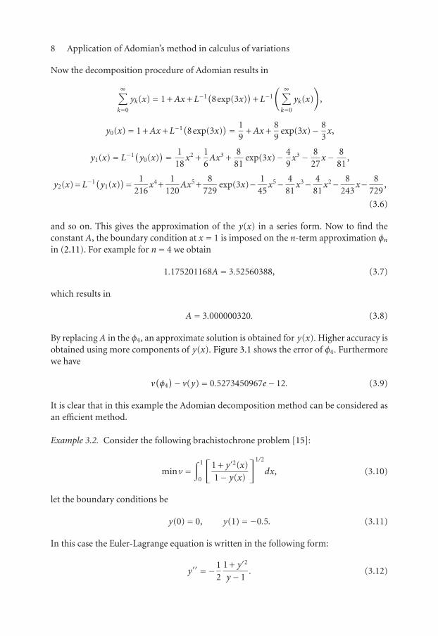
By replacing A in the φ4, an approximate solution is obtained for y(x). Higher accuracy isobtained using more components of y(x). Figure 3.1 shows the error of φ4. Furthermorewe have

v(φ4)− v(y)= 0.5273450967e− 12. (3.9)

It is clear that in this example the Adomian decomposition method can be considered asan efficient method.

Example 3.2. Consider the following brachistochrone problem [15]:

minv =∫ 1

0

[1 + y′2(x)1− y(x)

]1/2

dx, (3.10)

let the boundary conditions be

y(0)= 0, y(1)=−0.5. (3.11)

In this case the Euler-Lagrange equation is written in the following form:

y′′ = −12

1 + y′2

y− 1. (3.12)


2.5e − 07

2e − 07

1.5e − 07

1e − 07

5e − 08

00 0.2 0.4 0.6 0.8 1

x

Figure 3.1. Error function φ4− y(x) for 0≤ x ≤ 1.

By imposing the boundary condition at x = 1 on the four-term approximation

φ3 =3∑

k=0

yk (3.13)

and solving the resulted nonlinear equation, we obtain

A=−0.78503193483611740425. (3.14)

In this case we have

v(φ3)− v(y)= 0.2232e− 6, (3.15)

which shows the high accuracy of the method for nonlinear problems. Notice that thedirect methods for solving the variational problem provide an algebraic system of equa-tions. Solving such equations is very time consuming. But as we saw, using the decompo-sition procedure of Adomian, the solution of the problem is obtained very fast withoutsolving any algebraic system of equations.

Example 3.3. In this example we consider the following variational problem [16]:

minv =∫ π/2

0

(y′′2− y2 + x2)dx, (3.16)

that satisfies the conditions

y(0)= 1, y′(0)= 0, y(π

2

)= 0, y′

(π

2

)=−1. (3.17)


The corresponding Euler-Poisson equation is

y(4)− y = 0, (3.18)

or equivalently

y(x)= 1 +12!Ax2 +

13!Bx3 +L−1

4

(y(x)

), (3.19)

where L−14 is defined for a function h(x) by

L−14

(h(x)

)=∫ x

0

∫ t4

0

∫ t3

0

∫ t2

0h(t1)dt1dt2dt3dt4, (3.20)

in which A= y′′(0) and B = y(3)(0).Using the decomposition method we have

y0(x)= 1 +12!Ax2 +

13!Bx3,

y1(x)= L−14

(y0(x)

)= 124

x4 +1

720Ax6 +

15040

Bx7,

(3.21)

and so on. By imposing the boundary conditions at x = 1 on φ4, we obtain the followinglinear equations:

1.254589239A+ 0.6506494512B =−1.254589239,

1.650649451A+ 1.254589239B =−1.650649450,(3.22)

which results in

A=−1.000000001, B = 0.1254589241e− 8. (3.23)

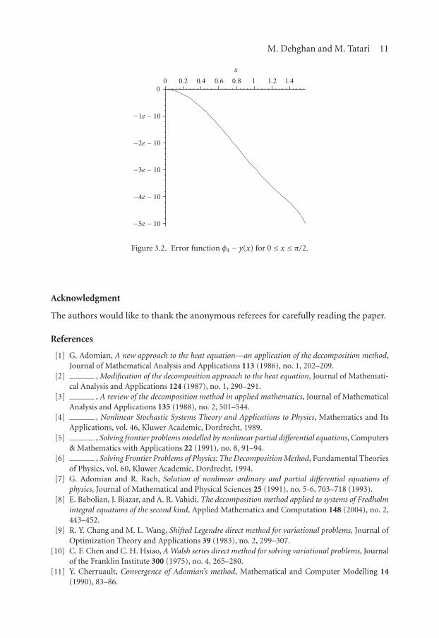
In Figure 3.2 the error function φ4− y(x) is plotted. Furthermore, we have

v(φ4)− v(y)=−0.4228e− 4. (3.24)

Obviously a better approximation can be found using more components of y(x).

4. Conclusion

Adomian decomposition method is used for finding the solution of the ordinary differ-ential equations which arise from problems of calculus of variations. It is also importantthat the Adomian decomposition method does not require discretization of the variables.It is not affected by computation round errors and one is not faced with necessity of largecomputer memory and time. The decomposition approach is implemented directly in astraightforward manner without using restrictive assumptions or linearization. Compar-ing the results with other works, the Adomian decomposition method was clearly reliableif compared with the grid point techniques where the solution is defined at grid pointsonly. It is important that this method unlike the most numerical techniques provides aclosed form of the solution.


0

−1e − 10

−2e − 10

−3e − 10

−4e − 10

−5e − 10

0 0.2 0.4 0.6 0.8 1 1.2 1.4

x

Figure 3.2. Error function φ4− y(x) for 0≤ x ≤ π/2.

Acknowledgment

The authors would like to thank the anonymous referees for carefully reading the paper.

References

[1] G. Adomian, A new approach to the heat equation—an application of the decomposition method,Journal of Mathematical Analysis and Applications 113 (1986), no. 1, 202–209.

[2] , Modification of the decomposition approach to the heat equation, Journal of Mathemati-cal Analysis and Applications 124 (1987), no. 1, 290–291.

[3] , A review of the decomposition method in applied mathematics, Journal of MathematicalAnalysis and Applications 135 (1988), no. 2, 501–544.

[4] , Nonlinear Stochastic Systems Theory and Applications to Physics, Mathematics and ItsApplications, vol. 46, Kluwer Academic, Dordrecht, 1989.

[5] , Solving frontier problems modelled by nonlinear partial differential equations, Computers& Mathematics with Applications 22 (1991), no. 8, 91–94.

[6] , Solving Frontier Problems of Physics: The Decomposition Method, Fundamental Theoriesof Physics, vol. 60, Kluwer Academic, Dordrecht, 1994.

[7] G. Adomian and R. Rach, Solution of nonlinear ordinary and partial differential equations ofphysics, Journal of Mathematical and Physical Sciences 25 (1991), no. 5-6, 703–718 (1993).

[8] E. Babolian, J. Biazar, and A. R. Vahidi, The decomposition method applied to systems of Fredholmintegral equations of the second kind, Applied Mathematics and Computation 148 (2004), no. 2,443–452.

[9] R. Y. Chang and M. L. Wang, Shifted Legendre direct method for variational problems, Journal ofOptimization Theory and Applications 39 (1983), no. 2, 299–307.

[10] C. F. Chen and C. H. Hsiao, A Walsh series direct method for solving variational problems, Journalof the Franklin Institute 300 (1975), no. 4, 265–280.

[11] Y. Cherruault, Convergence of Adomian’s method, Mathematical and Computer Modelling 14(1990), 83–86.


[12] M. Dehghan, Application of the Adomian decomposition method for two-dimensional parabolicequation subject to nonstandard boundary specifications, Applied Mathematics and Computation157 (2004), no. 2, 549–560.

[13] , The solution of a nonclassic problem for one-dimensional hyperbolic equation using thedecomposition procedure, International Journal of Computer Mathematics 81 (2004), no. 8, 979–989.

[14] , The use of Adomian decomposition method for solving the one-dimensional parabolicequation with non-local boundary specifications, International Journal of Computer Mathematics81 (2004), no. 1, 25–34.

[15] P. Dyer and S. R. McReynolds, The Computation and Theory of Optimal Control, Mathematics inScience and Engineering, vol. 65, Academic Press, New York, 1970.

[16] L. Elsgolts, Differential Equations and the Calculus of Variations, Mir, Moscow, 1977, translatedfrom the Russian by G. Yankovsky.

[17] I. M. Gelfand and S. V. Fomin, Calculus of Variations, revised English edition translated andedited by R. A. Silverman, Prentice-Hall, New Jersey, 1963.

[18] I. R. Horng and J. H. Chou, Shifted Chebyshev direct method for solving variational problems,International Journal of Systems Science 16 (1985), no. 7, 855–861.

[19] C. Hwang and Y. P. Shih, Laguerre series direct method for variational problems, Journal of Opti-mization Theory and Applications 39 (1983), no. 1, 143–149.

[20] N. Ngarhasta, B. Some, K. Abbaoui, and Y. Cherruault, New numerical study of Adomian methodapplied to a diffusion model, Kybernetes 31 (2002), no. 1, 61–75.

[21] M. Razzaghi and M. Razzaghi, Fourier series direct method for variational problems, InternationalJournal of Control 48 (1988), no. 3, 887–895.

[22] , Instabilities in the solution of a heat conduction problem using Taylor series and alternativeapproaches, Journal of the Franklin Institute 326 (1989), no. 5, 683–690.

[23] M. Tatari and M. Dehghan, Numerical solution of Laplace equation in a disk using the Adomiandecomposition method, Physica Scripta 72 (2005), no. 5, 345.

[24] A.-M. Wazwaz, A reliable modification of Adomian decomposition method, Applied Mathematicsand Computation 102 (1999), no. 1, 77–86.

[25] , A new algorithm for calculating Adomian polynomials for nonlinear operators, AppliedMathematics and Computation 111 (2000), no. 1, 53–69.

[26] , Approximate solutions to boundary value problems of higher order by the modified decom-position method, Computers & Mathematics with Applications 40 (2000), no. 6-7, 679–691.

[27] , The numerical solution of fifth-order boundary value problems by the decompositionmethod, Journal of Computational and Applied Mathematics 136 (2001), no. 1-2, 259–270.

[28] , The numerical solution of sixth-order boundary value problems by the modified decompo-sition method, Applied Mathematics and Computation 118 (2001), no. 2-3, 311–325.

Mehdi Dehghan: Department of Applied Mathematics, Faculty of Mathematics andComputer Science, Amirkabir University of Technology, 424 Hafez Avenue,Tehran 15875-4413, IranE-mail address: [email protected]

Mehdi Tatari: Department of Applied Mathematics, Faculty of Mathematics andComputer Science, Amirkabir University of Technology, 424 Hafez Avenue,Tehran 15875-4413, IranE-mail address: [email protected]

mailto:[email protected]

mailto:[email protected]

Submit your manuscripts athttp://www.hindawi.com

Hindawi Publishing Corporationhttp://www.hindawi.com Volume 2014

MathematicsJournal of


Mathematical Problems in Engineering

Hindawi Publishing Corporationhttp://www.hindawi.com

Differential EquationsInternational Journal of

Volume 2014

Applied MathematicsJournal of


Probability and StatisticsHindawi Publishing Corporationhttp://www.hindawi.com Volume 2014

Journal of


Mathematical PhysicsAdvances in

Complex AnalysisJournal of


OptimizationJournal of


CombinatoricsHindawi Publishing Corporationhttp://www.hindawi.com Volume 2014

International Journal of


Operations ResearchAdvances in

Journal of


Function Spaces

Abstract and Applied AnalysisHindawi Publishing Corporationhttp://www.hindawi.com Volume 2014

International Journal of Mathematics and Mathematical Sciences


The Scientific World JournalHindawi Publishing Corporation http://www.hindawi.com Volume 2014


Algebra

Discrete Dynamics in Nature and Society



Decision SciencesAdvances in

Discrete MathematicsJournal of

Hindawi Publishing Corporationhttp://www.hindawi.com

Volume 2014 Hindawi Publishing Corporationhttp://www.hindawi.com Volume 2014

Stochastic AnalysisInternational Journal of

the use of adomian decomposition method for solving...

Documents