the utility of contrast-enhanced ultrasound in the ... utility of contrast-enhanced ultrasound in...
TRANSCRIPT
The Utility of Contrast-Enhanced Ultrasound in the
Assessment of Solid Small Renal Masses
By
Leila Tabatabaeifar
A thesis submitted in conformity with the requirements
For the degree of Master of Science
Institute of Medical Science
University of Toronto
2013
Copyright by Leila Tabatabaeifar, 2013
The Utility of Contrast-Enhanced Ultrasound in the Assessment of Solid Small Renal Masses

ii
The Utility of Contrast-Enhanced Ultrasound in the
Assessment of Solid Small Renal Masses
Leila Tabatabaeifar
Master of Science
Institute of Medical Science
University of Toronto
2013
Abstract
Purpose: To compare hemodynamic of malignant and benign SRMs on CT and CEUS.
Method: Seventy biopsy proven SRM underwent CEUS. Sixty-three had CT. After injection of
0.2 ml of Definity, 3min and after 0.9 ml infusion, 30 sec of data were acquires. Lesion
hemodynamics relative to the cortex was evaluated both qualitatively and quantitatively.
Results: Considering 15 and 20 HU as enhancement threshold, 10% to 13% of patients did not
enhance on CT, while all lesions enhanced on CEUS. Papillary RCCs showed hypovascularity
with 100% specificity. In other RCCs, PI, WI slope 5 to45%, 50 to100%, 10 to 90%, WO slope
100 to 50%, 100 to 10%, WO intensity at peak+30 seconds were statistically higher than benign
SRMs.
iii
Conclusion: All solid SRMs enhance on CEUS, while CT does not show vascularity in 10-13%
of solid SRMs. CEUS can differentiate malignant from benign SRMs by evaluating their
hemodynamics.
Key words: Contrast-enhanced ultrasound, microbubble contrast agent, solid small renal mass,
kidney, cancer, Definity.
iv
Acknowledgement
I have three strong-minded men to thank deeply; Dr. Mostafa Atri, Dr. Narinder Paul, and
Dr. Masoom Haider, and it has been an honor to be their pupil.
Dr. Atri, I would like to thank you for trusting me with the CEUS project, even though my
Clinical and physics knowledge on and experience on radiology were little. It was very exciting
to be in charge of this study, look for eligible cases, explain the study to them, and perform
clinical trials, and finally to see the results of our experiment. In this long journey, I not only
learnt a lot about Small Renal Masses, and Contrast Enhanced Ultrasound, but I also practiced to
not sacrifice the ethics in the favor of research.
Dr. Narinder Paul, I would like to thank you sincerely for your support and guidance throughout
this project that has given me the strength to not give up. You have been my guiding light and
my mentor since the beginning.
Dr. Masoom Haider, I would like to thank you, and show my appreciation for accepting to be
part of my committee and guiding me through this study, in spite of your very busy schedule.
I want to acknowledge with deep gratitude the contributions of urologists, Dr. Michael Jewett
and Dr. Antony Finelli for letting me participate in their clinics to accrue patients.
I also would like to thank the summer medical student, Derek Sue-Chu-lam, for his great support
and enthusiasm about this project.
This study would not been accomplished without help and support of Ultrasound technicians of
Toronto General Hospital.

v
I also appreciate University Health Network (UHN) and Lantheus Medical Imaging Inc. for their
financial support of this study.
vi
Dedication
To all that I dearly LOVE …
vii
TABLE OF CONTENTS
Abstract…………………………………………………………….…………………………….ii
Acknowledgements…………………………………………………….…………………...…...iv
Dedication………………………………..…….…………………...……………………………vi
Table of Contents……………………………………………….………………………………vii
List of Figures…………………………………………………………………………………...xi
List of Tables…………………………………………………………………………………...xiii
List of Abbreviations…………………………………………………………………………...xv
Chapter 1: Literature Review……………………………………………...…………..………..1
1. Kidneys……………………………………..………..………………………………..……1
1.1 Anatomy………………………………………………………..……………..………1
1.2 Blood Supply……....…………………………………….…….……………..………3
1.3 Histology………………………………………………………….……………..……4
1.4 Innervation……………………………………………………………………..……..4
1.5 Function…………………………………………………………………………..…..4
2. Small Renal Masses…………………………………………………………………………5
2.1 Solid Renal Masses………………………………………….………………..………6
2.2 Renal Cell Carcinoma………………………………………………………..……….7
2.2.1 Definition……………………………………….……………..….…………….7
2.2.2 Pathophysiology……………………………………..………….……..………..8
2.2.3 Etiology and Risk Factors…………………………….……….……..…………8
2.2.4 Common Subtypes……………………………………..……..……………..….9
2.2.4.1 Conventional Clear Cell RCC (CCRCC)…………….……………......…9
2.2.4.2 Papillary RCC……………………………………….…...……...………11
2.2.4.3 Chromophobe RCC…………………………………………...…………12
2.2.5 Signs and Symptoms…………………………….……...………….………….14
2.2.6 Prevalence and Incidence……………………………………….……………..14
viii
2.2.7 Health Expenses in Canada………………………………………………...…15
2.2.8 Ultrasound…………………………………………..…………………………16
2.2.8.1 Contrast-Enhanced Ultrasound (CEUS)….………………..…………….17
2.2.8.2 Physics of CEUS..…………………………………………………….…20
2.2.8.3 Harmonic Ultrasound……………………………………….……………21
2.2.8.4 Pulse Inversion Harmonic Imaging………………………………..…….23
2.2.8.5 Mechanical Index …………………………………….…………………24
2.2.8.6 Applications ………………………………………………….………….26
3. Ultrasound Contrast Agents …………………………………………………………………..28
3.1 Definity ……………………………………………………………..………………30
3.1.1 Bolus Administration …………………………………………..………….31
3.1.2 Infusion ……………………………………………………………...…….31
4. Tumour Vasculature………………………………………………………………………….. 31
5. Previous Studies…………………………………………………..…………..………………32
Chapter 2: Research Aims and Hypotheses……………..…………………..………………..35
1. Hypothesis…………………………………………..……………………………….35
2. Objectives……………………………………….…….……………………………..35
2.1 Primary Objective…………………………….……….…………………………35
2.2 Secondary objective…………………….………………………………………..36
Chapter 3: Methods…………………………………………………………………………….37
1. Study population ……………………………………….……………..…….…………… 37
1.1 Inclusion Criteria……………………………………………………..…………37
1.2 Exclusion Criteria………………………………………………………….……37
1.3 Patient Population………….……………………………………………………38
2. Ultrasound Examination………………………………………………...……………41
2.1 B-Mode Ultrasound……..………………………………………………………41
2.2 Contrast Enhanced Ultrasound…………………………………...…………..…41
2.2.1 First Bolus Injection……………………………………………….………43
2.2.2 Second Bolus Injection……………………………………………………43
2.2.3 Infusion…………………………………………………………....………43
3. Computed Tomography (CT) Examination …………………………………………..46
4. Data Collection and Analysis………………………………………………….…..…47
ix
4.1 Qualitative Data Analysis…………………………………………………….…47
4.2 Quantitative Data Analysis…………………………………………….………..48
4.2.1 Quantitative Analysis of Philips IU22 Data……………………………....48
4.2.1.1 Bolus Phase…………………………………………………….……48
4.2.1.2 Important TIC Parameters ……………………………………….…51
4.3 Additional Analysis………………………………………………………….….52
4.4 Data Normalization …………………………………….…………….………….52
4.5 Statistical Analysis of Data……………………….…………………..…………53
4.6 Student’s role in the study………………..…………………………………..55
Chapter 4: Results…………………………………………..….……………………………….57
1. Study Population………………………………..……………..………….…………..57
2. Qualitative Variables ……………………………..………….……………………....58
2.1 Enhancement of solid SRM on CT and CEUS ………………….….………58
2.2 Unenhanced US …………………………………………………………….59
3. Contrast Enhanced Ultrasound (CEUS)………………………………………………64
4. Quantitative Assessment of SRM with QLAB ……………………………..………75
4.1 Quantitative Variables ……………………………………………………..……….75
4.2 Removing Papillary and Comparing Malignant with Benign Tumors …….……76
5. Infusion results ……………………………..…………………………………..……..78
6. CT Subjective Data …………………………………………………….………..……78
7. Logistic Regression Models……………………………………………………..…….83
7.1 Wash-in Variables……………………………………………………………83
7.2 Wash-out Variables…………………………………………………………..84
7.3 Combining Wash-in and Wash-out Variables……………………………….85
7.4 Qualitative Variables- Unenhanced US….…………………………………..85
7.5 Qualitative Variables- Enhanced US……………….………………………..85
7.6 Qalitative Variables- CT data………………………………………………. 86
7.7 Qualitative Variables - Unenhanced US, Enhanced US and CT…………….86
7.8 Combining Qualitative and Quantitative Variables………………………… 87
8. Summary of Results ……………………………………………………....…………..88
x
Chapter 5: Discussion………………………………………………………………….……….89
1. Qualitative Findings…………………………………………...………….………….89
1.1 Echotexture……………………………………..…………………….……….....90
1.2 Halo………………………………………………………………………………90
1.3 Heterogeneity…………………………………………………………………….91
1.4 Vascular enhancement …………………………………………..………………91
1.5 Vascular Pattern…………………………………………..……………………...92
1.6 Wash-out…………………………………………………………………………93
1.7 Tumor Heterogeneity …………………………………..………………………..93
1.8 Pseudocapsule ………………………………………..………………………….94
2. Quantitative Findings……………………………………..…………………….……94
3. Logistic Regression Model………………………………………….……………….97
Chapter 6: Conclusion………………………………………………...…..……………………99
Chapter 7: Future Directions………………………………………………………...………100
1. Strengths ………………………………………………..………………………..…100
2. Limitations ……………………………………………….……………………...…..100
3. Future Work…………………………………………....……………………….……101
References………………………………………...………………………………………..…105
xi
List of Figures
Figure 1. Genitourinary and Excretory system………....…………………………...…...………..2
Figure 2. Anatomy of the Kidney……………………………………………..……….………….3
Figure 3. Nephron Structure …………………………………………...……..…………………..5
Figure 4. Gross Specimen of a Clear Cell RCC……………………..….…………..……………10
Figure 5. Photomicrograph of a Clear Cell RCC………………..…….………………...……….10
Figure 6. Gross Specimen of a Papillary RCC………………………..……………..…………..11
Figure 7. Photomicrograph of a Type 1 Papillary RCC……………………..…………….……..12
Figure 8. Gross Specimen of a Chromophobe RCC………………………….………….………13
Figure 9. Photomicrograph of a Chromophobe RCC……….…………………………..……….13
Figure 10. Incidental acoustic wave………...……………………………………………..……..21
Figure 11. Pulse inversion………………………………………………………...………...……24
Figure 12. Harmonic signal enhancement with pulse inversion ……...………………………....25
Figure 13. Microbubble fragmentation ………………...……………….……………………….29
Figure 14. A flow diagram of SRM distribution……………………….………………..……….40
Figure 15. Flow diagram of CEUS test step by step…………...…………………………….…..45
Figure 16. TIC of a bolus phase CEUS ………………………...………………………………..50
Figure 17. TIC of an infusion phase CEUS …………...………………………………….……..50
Figure 18. Patients’ demographic data in a histogram bar ………...…………………….………57
Figure 19. A papillary tumor on B-mode US and CEUS……..………………...……………….65
Figure 20. TIC of a papillary tumor …………………………………………………….……….66
xii
Figure 21. An Oncocytoma tumor on B-mode US and CEUS …………...……………………..71
Figure 22. TIC of an Oncocytoma tumor …………………………………...………..………….71
Figure 23. A CCRCC tumor on B-mode US and CEUS …………….……..…………......…….72
Figure 24. TIC of a CRCC tumor ………………………………..…………………...…………72
Figure 25. A flow diagram of an algorithm to differentiate malignant from benign SRM …......98
xiii
List of Tables
Table 1. Reported doses for microbubble contrast agents…………………..………..…………30
Table 2. Demographic Data of lesions……………………………………….………………….39
Table 3. Solid SRM enhancements on CT and CEUS ……………………...…………………..59
Table 4. Lesion Echotexture………………………………………………………………..……60
Table 5. Lesion Echotexture (summarized)……………...……………...……………………….61
Table 6. Heterogeneity ………………………………….……………………………….………61
Table 7. Halo……………………….……………………………………………………….……62
Table 8. Tumor Size……………………………………………………………………...………62
Table 9. Ultrasound features……….....……………………………………….…………………63
Table 10. Vascularity compared to renal cortex ……………………………………………...…64
Table 11. Vascularity compared to renal cortex (summarized)……...……….……………….…65
Table 12. Vascular Pattern of the renal mass …………….……..……………….………………66
Table 13. Vascular Pattern of the renal mass ………………………………..……..……………67
Table 14. Vascular Heterogeneity of the renal mass………………………………….…………68
Table 15. Post-Contrast Halo ……………………………………………………………………68
Table 16. Wash-out ……………….…………………………………….……………………….69
Table 17. Summary of qualitative features on ultrasound …………..…………………………..70
Table 18. Hypovascularity pattern on CEUS (1) …………………..……………………………73
Table 19. Hypovascularity pattern on CEUS (2) …………………….………………………….74
Table 20. Summary………………………………………………………………………………74
Table 21. Quantitative parameters.………………………………………………………………75
xiv
Table 22. Quantitative parameters positive results …………….…………………………..……77
Table 23. Quantitative values of infusion TIC……….……..………………………………..…..78
Table 24. CT population ……………………..…………………………………………….……79
Table 25. Heterogeneity.…………………………………………………………………………79
Table 26. Lesions vascularity on nephrographic phase.…………………………………………80
Table 27. Lesion vascularity on CT…….…………………………………..…….………...……80
Table 28. Nephrographic vs. Arterial Phase Tumor Vascularity ……..…………………..……..81
Table 29. Vascular Heterogeneity ……...………………………………………………………..81
Table 30. Wash-Out of Tumor Contrast………...……………………………………...………..82
Table 31. Summary ……………………………………………………………..………….……82
xv
List of Abbreviations
AML Angiomyolipoma
AUC Area Under the Curve
BHDS Birt-Hogg-Dube Syndrome
CEUS Contrast-Enhanced Ultrasound
CCRCC Clear Cell Renal Cell Carcinoma
CHIQ Contrast Harmonic Imaging Quantification
CT Computed Tomography
FRO Familial Renal Oncocytoma
HPRC Hereditary Papillary Renal Carcinoma
HRC Hereditary Renal Carcinoma
LDRW Local Density Random Walk
MB Microbubbles
MI Mechanical Index
MRI Magnetic Resonance Imaging
NCI National Cancer Institute
PI Peak Intensity
RAML Renal Angiomyolipoma
RBC Red Blood Cell
xvi
RCC Renal Cell Carcinoma
ROI Region of Interest
SRM Small Renal Masses
TIC Time Intensity Curve
TOST Two-One Sided Test
TPH1/2 Time from Peak to Half of the Wash-Out slope
TTP Time to Peak
US Ultrasound
USCA Ultrasound Contrast Agent
VHL Von Hippel-Lindau
WI Wash-In
WO Wash-Out
1
Chapter 1
Literature Review
1. Kidneys
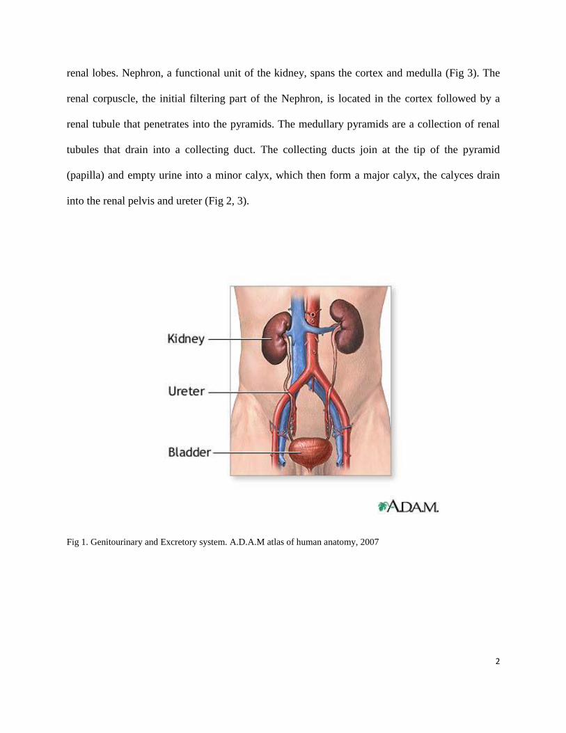
Human beings owe their physical health to organs and systems functioning properly
together. Kidneys are the most important organs of the genitourinary/excretory system (Fig
1).
1.1 Anatomy
Located in the abdominal cavity‟s para-vertebral gutter, the left kidney sits approximately at
the vertebral level T12 to L3, with the right kidney slightly lower, due to an asymmetry within
the abdominal cavity caused by the liver. Since the superior borders of the both kidneys are
adjacent to the liver and the spleen respectively, both move down on inhalation. The kidneys
and adrenal glands resting superior to it are surrounded by para and perirenal fat. The kidney
itself is covered by a tough fibrous capsule and perirenal fat by a fascia called Gerota. Each
kidney weighs between 115 and 170 grams in an adult and measures 11-14cm in length, 6cm
wide, and 4cm thick; the left kidney being slightly larger [1] . Its concave and convex surfaces
give it a kidney bean shape. The renal hilum contains the renal artery, vein, and ureter on its
concave surface (Fig 1, 2).
The kidney is formed by superficial (Cortex) and deep (Medulla) structures. The medulla
itself contains 8 to 18 pyramids of Malpighi, which together with surrounding renal cortex form
2
renal lobes. Nephron, a functional unit of the kidney, spans the cortex and medulla (Fig 3). The
renal corpuscle, the initial filtering part of the Nephron, is located in the cortex followed by a
renal tubule that penetrates into the pyramids. The medullary pyramids are a collection of renal
tubules that drain into a collecting duct. The collecting ducts join at the tip of the pyramid
(papilla) and empty urine into a minor calyx, which then form a major calyx, the calyces drain
into the renal pelvis and ureter (Fig 2, 3).
Fig 1. Genitourinary and Excretory system. A.D.A.M atlas of human anatomy, 2007
3
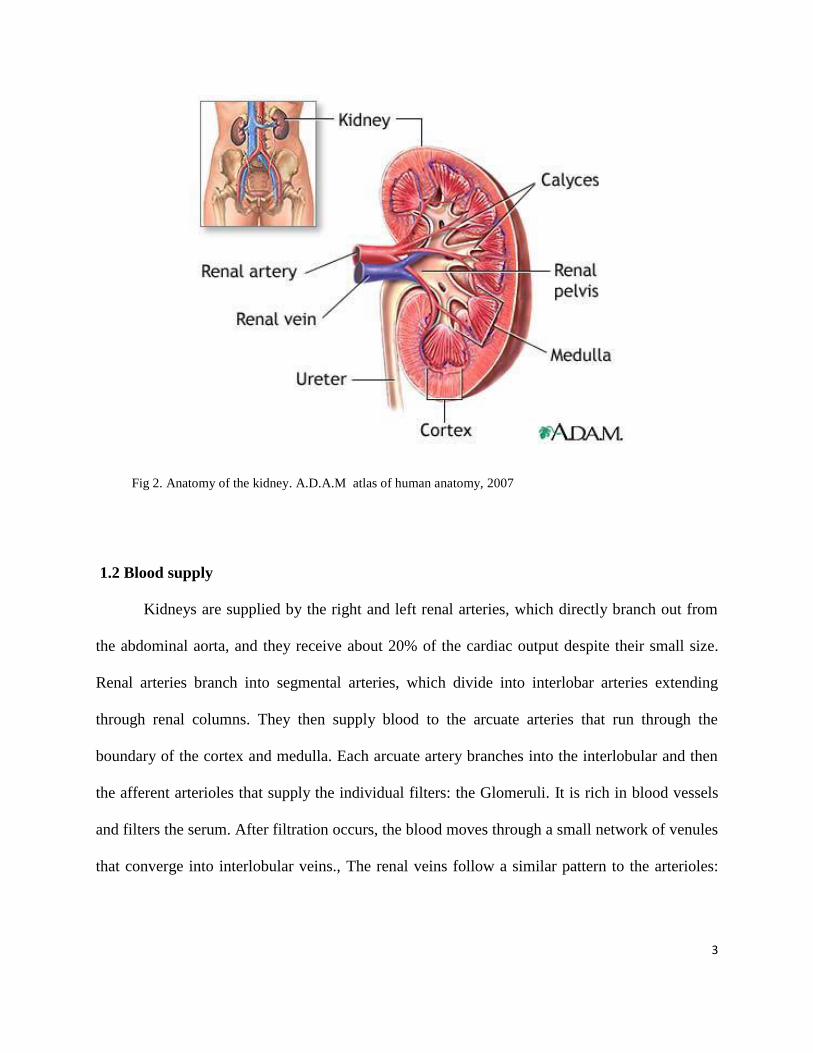
Fig 2. Anatomy of the kidney. A.D.A.M atlas of human anatomy, 2007
1.2 Blood supply
Kidneys are supplied by the right and left renal arteries, which directly branch out from
the abdominal aorta, and they receive about 20% of the cardiac output despite their small size.
Renal arteries branch into segmental arteries, which divide into interlobar arteries extending
through renal columns. They then supply blood to the arcuate arteries that run through the
boundary of the cortex and medulla. Each arcuate artery branches into the interlobular and then
the afferent arterioles that supply the individual filters: the Glomeruli. It is rich in blood vessels
and filters the serum. After filtration occurs, the blood moves through a small network of venules
that converge into interlobular veins., The renal veins follow a similar pattern to the arterioles:
4
the interlobular veins provide blood to the arcuate veins, which then flows back to the interlobar
veins to form the renal vein exiting the kidney [2] (Fig 2).
1.3 Histology
Studying the structure of the kidney under a microscope, various distinct cell types occur in
the kidney: they include the renal glomerulus parietal cell, glomerulus podocyte, proximal,
tubule brush border cell, loop of henle thin segment cell, thick ascending limb cell, kidney distal
tubule cell, collecting duct cell, and interstitial cells. Each of these cell types can be the origin of
different disease and malignancies and can lead to renal dysfunction [2].
1.4 Innervation
The renal plexus connects the kidney to the nervous system and contains sensory and
sympathetic nerves, which course along the renal artery into the kidney. The sympathetic
nervous system triggers vasoconstriction and therefore a reduction in renal flow. The sensory
input, from the T10-11 levels of the spinal cord, is responsible for transferring sensation and pain
to the flank and the corresponding dermatome. The kidneys do not receive input from the
parasympathetic nervous system [3].
1.5 Function
Kidneys, as the most important part of the excretory system, participate in whole body
homeostasis, regulation of acid-base balance, electrolyte concentrations, extracellular fluid
volume, and regulation of blood pressure both independently and in concert with other organs,
particularly the endocrine system. Filtration, reabsorption, and secretion are mechanisms which
5
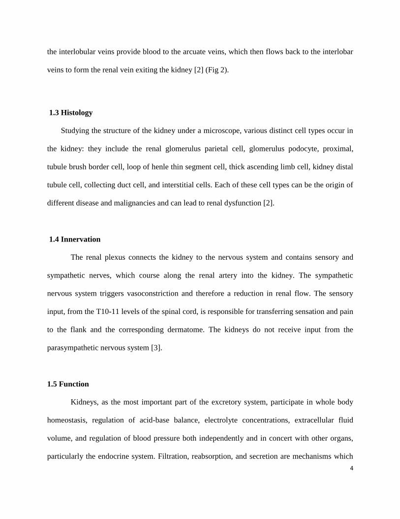
take place in the nephron, the kidney‟s smallest functional unit. Kidneys filter 180 liters of fluid
a day, most of which is reabsorbed and produce about 2 liters of urine daily [3] (Fig 3).
Fig 3. Nephron structure. Encyclopedia Britannica 2006.
2. Small Renal Masses
Approximately 13 to 27% of abdominal imaging studies identify an incidental renal
lesion [4, 5]. The majority of these lesions are small, simple cysts that do not show enhancement
after the administration of intravenous contrast material, and require no treatment [4, 5].
A minority of small renal masses are solid masses or complex cystic masses, which show
contrast enhancement on CT or MRI and could represent cancer. An enhancing mass is described
on CT when there is an increase in density of at least 15 Hounsfield units after the administration
6
of contrast material [4]. For the purposes of this thesis, a small renal mass (SRM) is defined as a
contrast-enhancing mass with a largest dimension of 4 cm on cross sectional imaging.
There is an increase in detection of incidental SRM due to the increased use of cross
sectional imaging modalities for screening and diagnostic purposes. This has led to a 126%
increase in the detection of renal masses [5]. From 1988 to 2003, the incidence of SRM increased
relative to other renal tumors, and they now make up 48 to 66% of all renal tumors that are
diagnosed, and 38% of all renal tumors that are excised [6], [7] Often the patient is
asymptomatic. When an incidental SRM is identified on imaging, the management challenge
involves distinguishing a benign mass from one that is likely to be malignant, and then
determining the appropriate treatment for malignant masses.
2.1 Solid Renal Masses
Masses that have measurable contrast enhancement on CT or MRI are classified as solid
masses or complex cystic masses (Bosniak class III or class IV) [8, 9]. Almost 80% of enhancing
lesions are malignant [10]. In studies that involve relatively short-term follow-up (≤3 years), the
reported growth rate is similar for malignant and benign tumors (oncocytoma) [11, 12]. In one
meta-analysis, 30% of small renal masses showed no growth over an observation period of 23 to
39 months [11]. Masses that showed no growth (83%) were as likely to be malignant as were
those that grew (89%) (P>0.05) [13]. This finding confirms that lesion growth by itself cannot
predict the underlying histological nature of the mass. Additionally, there is no definitive clinical
or radiologic characteristics that effectively predict future growth; neither size at presentation nor
the final histological diagnosis (even if it is proven renal-cell carcinoma) correlates with growth
rate [11].
7
Small renal masses are referred to solid renal tumors that show enhancement on computed
tomography (CT) and magnetic resonance imaging (MRI), and are suspected of being renal cell
carcinomas. Nowadays, most SRM are detected incidentally on CT or MRI done for different
abdominal symptoms. Each year 20,000 to 30,000 new cases are diagnosed in the United States,
and the rate is rising by 3% to 4% per year as a result of increased utility of CT and MRI [14-
16].
Regarding their size, Small Renal Masses are defined as tumors less than 4 cm in their largest
diameter. However, Strict definition of SRM is lacking; 4 cm is considered as cut-off, imported
from the classical one regarding partial surgery of the kidney and TNM classification [17, 18].
2.2 Renal Cell Carcinoma
2.2.1 Definition
Renal Cell Carcinoma (RCC) is described as a cancer that develops in the lining of the
renal tubules (Merriam-Webster Medical Dictionary). It is also called renal cell cancer. The
National Cancer Institute defines RCC as a cancer that forms in the tissues of the kidneys.
Kidney cancer includes RCC (a cancer that forms in the lining of very small tubules) and
transitional cell carcinoma (a cancer that forms in the urothelium of the kidney where urine
collects). It also includes „Wilms tumor,‟ a type of kidney cancer that usually develops in
children under the age of 5 (National Cancer Institute).
8
2.2.2 Pathophysiology
The tissue of origin for RCC is the proximal renal tubular epithelium. RCC occurs in a
sporadic (nonhereditary) and a hereditary form, and both forms are associated with structural
alterations of the short arm of chromosome 3 (3p). At least four hereditary syndromes associated
with renal cell carcinoma are recognized: von Hippel-Lindau (VHL) syndrome, hereditary
papillary renal carcinoma (HPRC), and hereditary renal carcinoma (HRC).
2.2.3 Etiology
The following environmental and genetic factors have been studied as possible causes for
renal cell carcinoma:
Cigarette smoking doubles the risk of renal cell carcinoma and contributes to as many as
one third of all RCC. The risk appears to be dose-dependent as it increases with the amount
of cigarette smoking [19].
Obesity is another risk factor, particularly in women; increasing body weight has a linear
relationship with increased risk [20].
Hypertension may be associated with an increased incidence of renal cell carcinoma [21].
Phenacetin-containing analgesia taken in large amounts may be associated with increased
incidence of renal cell carcinoma [22, 23].
In patients undergoing long-term renal dialysis, there is an increased incidence of acquired
cystic disease of the kidney, which predisposes to renal cell cancer [24].
In renal transplant recipients, acquired renal cystic disease of the native kidney also
predisposes to renal cell cancer [25, 26].
9
Some case-control studies have shown that RCC shows more prevalence in persons with
low socioeconomic status and urban background, However those studies have not
defined the causative factors [27, 28]. The modern Western diet, which contains high
amount of fat and protein, but low amount of fruits and vegetables, might have some role
in increasing the incidence of RCC. Also high intake of dairy products and increased
coffee or tea have been associated with RCC [19, 21, 28].
A family history of RCC may also be a factor. Some study show a high increase of risk
(relative risk of 2.9) for individuals whom their first- or second-degree relative was
diagnosed with RCC [23].
2.2.4 Common subtypes
2.2.4.1 Clear Cell RCC
Previously referred to as conventional RCC, clear cell RCC is the most common
histologic subtype, accounting for 70% of all RCC (National Cancer Institute). Clear cell RCC
recapitulates the epithelium of the proximal convoluted tubules [29]. The intracytoplasmic
glycogen and lipids are dissolved during histological processing, rendering the cells “clear”
(National Cancer Institute).
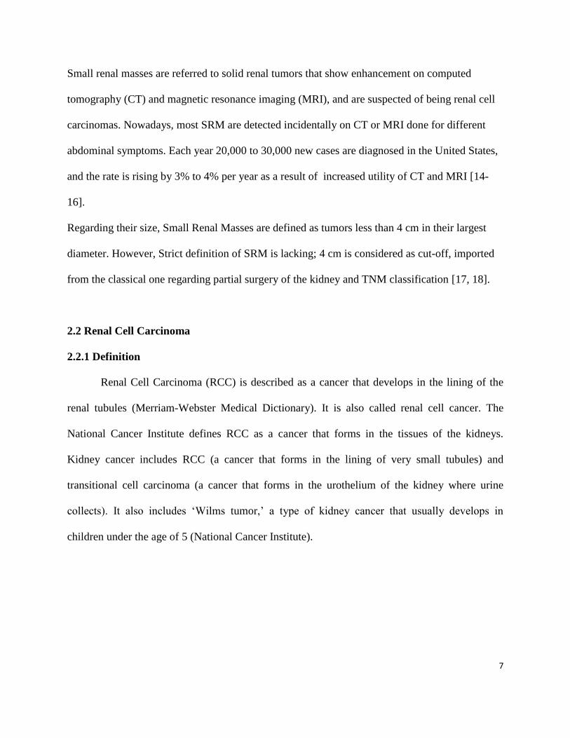
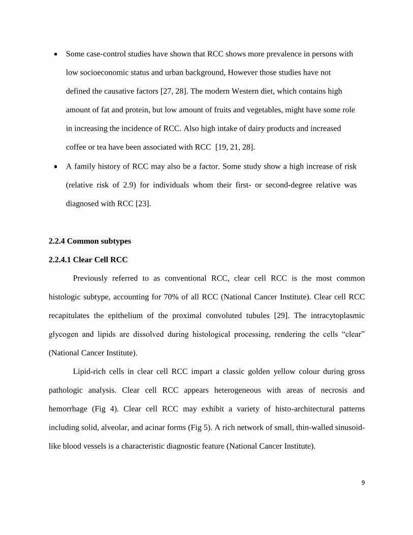
Lipid-rich cells in clear cell RCC impart a classic golden yellow colour during gross
pathologic analysis. Clear cell RCC appears heterogeneous with areas of necrosis and
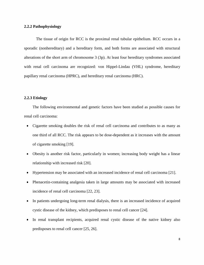
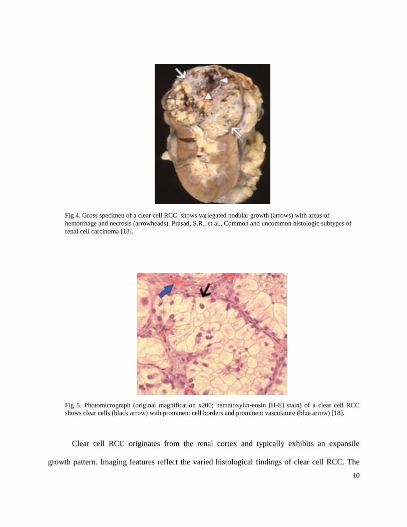
hemorrhage (Fig 4). Clear cell RCC may exhibit a variety of histo-architectural patterns
including solid, alveolar, and acinar forms (Fig 5). A rich network of small, thin-walled sinusoid-
like blood vessels is a characteristic diagnostic feature (National Cancer Institute).
10
Fig 4. Gross specimen of a clear cell RCC shows variegated nodular growth (arrows) with areas of
hemorrhage and necrosis (arrowheads). Prasad, S.R., et al., Common and uncommon histologic subtypes of
renal cell carcinoma [18].
Fig 5. Photomicrograph (original magnification x200; hematoxylin-eosin [H-E] stain) of a clear cell RCC
shows clear cells (black arrow) with prominent cell borders and prominent vasculature (blue arrow) [18].
Clear cell RCC originates from the renal cortex and typically exhibits an expansile
growth pattern. Imaging features reflect the varied histological findings of clear cell RCC. The
11
presence of hemorrhage, necrosis, and cysts commonly make clear cell RCC appear
heterogeneous during imaging. Multicentricity and bilaterality are rare (<5%) in sporadic cases
[30].
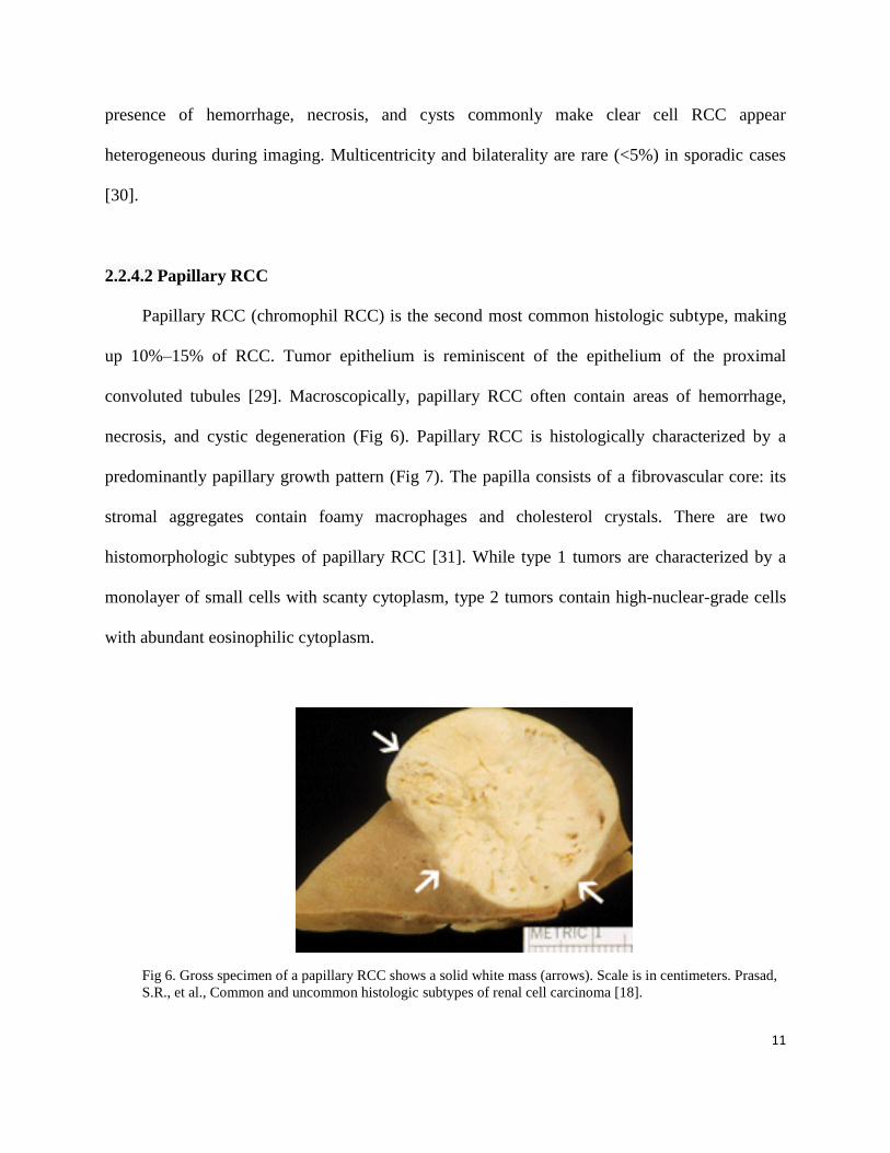
2.2.4.2 Papillary RCC
Papillary RCC (chromophil RCC) is the second most common histologic subtype, making
up 10%–15% of RCC. Tumor epithelium is reminiscent of the epithelium of the proximal
convoluted tubules [29]. Macroscopically, papillary RCC often contain areas of hemorrhage,
necrosis, and cystic degeneration (Fig 6). Papillary RCC is histologically characterized by a
predominantly papillary growth pattern (Fig 7). The papilla consists of a fibrovascular core: its
stromal aggregates contain foamy macrophages and cholesterol crystals. There are two
histomorphologic subtypes of papillary RCC [31]. While type 1 tumors are characterized by a
monolayer of small cells with scanty cytoplasm, type 2 tumors contain high-nuclear-grade cells
with abundant eosinophilic cytoplasm.
Fig 6. Gross specimen of a papillary RCC shows a solid white mass (arrows). Scale is in centimeters. Prasad,
S.R., et al., Common and uncommon histologic subtypes of renal cell carcinoma [18].
12
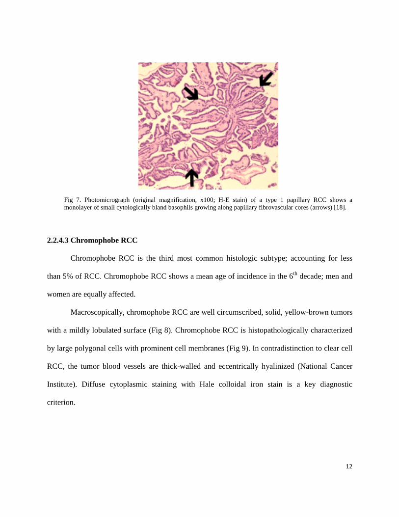
Fig 7. Photomicrograph (original magnification, x100; H-E stain) of a type 1 papillary RCC shows a
monolayer of small cytologically bland basophils growing along papillary fibrovascular cores (arrows) [18].
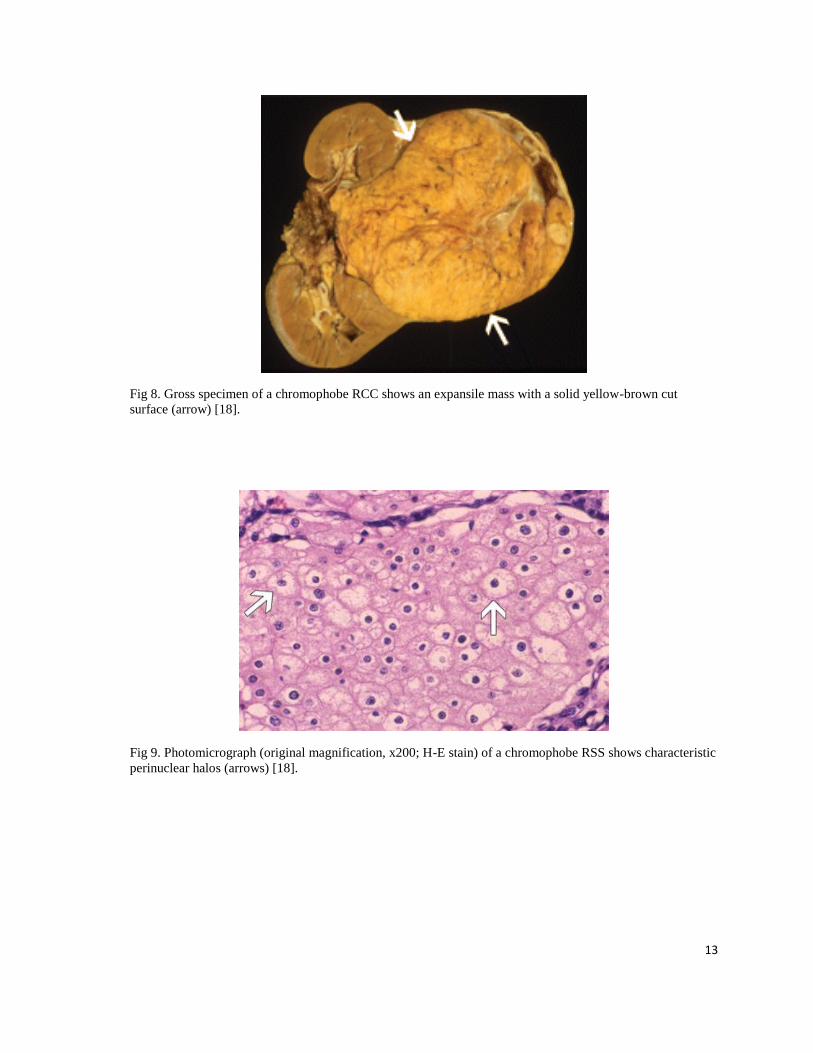
2.2.4.3 Chromophobe RCC
Chromophobe RCC is the third most common histologic subtype; accounting for less
than 5% of RCC. Chromophobe RCC shows a mean age of incidence in the 6th
decade; men and
women are equally affected.
Macroscopically, chromophobe RCC are well circumscribed, solid, yellow-brown tumors
with a mildly lobulated surface (Fig 8). Chromophobe RCC is histopathologically characterized
by large polygonal cells with prominent cell membranes (Fig 9). In contradistinction to clear cell
RCC, the tumor blood vessels are thick-walled and eccentrically hyalinized (National Cancer
Institute). Diffuse cytoplasmic staining with Hale colloidal iron stain is a key diagnostic
criterion.
13
Fig 8. Gross specimen of a chromophobe RCC shows an expansile mass with a solid yellow-brown cut
surface (arrow) [18].
Fig 9. Photomicrograph (original magnification, x200; H-E stain) of a chromophobe RSS shows characteristic
perinuclear halos (arrows) [18].

14
2.2.5 Signs and Symptoms
Many renal cell carcinoma (RCC) may remain asymptomatic and undetectable for most
of their course [32, 33]. The classic triad, which includes flank pain, gross hematuria, and
palpable abdominal mass, is uncommon (about 10%) [33, 34], and more than half of RCCs are
detected incidentally during the utility of medical imaging modalities for unrelated purposes [33,
35].
Thirty percent of patients with symptomatic RCCs show paraneoplastic syndrome.
Paraneoplastic syndrome is described as a collection of symptoms and signs that result from
substances produced by the tumor. Most common syndromes seen in RCC are hypertension,
cachexia, weight loss, pyrexia, neuromyopathy, amyloidosis, elevated erythrocyte sedimentation
rate, anemia, abnormal liver function, hypercalcemia, and polycythemia [33]. If the disease
reaches the end stage and metastasizes to other organs such as bone and lungs, patients might
present symptoms such as bone pain and persistent cough [32, 33].
2.2.6 Prevalence and incidence
Renal cell carcinoma, the most common primary malignancy of the kidney, accounts for
approximately 3 to 4% of adult malignancies [33, 36], 2.3% of cancer mortality, and 90-95% of
kidney neoplasms. Most adult kidney cancers that originate from the renal parenchyma are renal
cell carcinomas (RCC) [37].
Renal cell carcinoma is more common in people of Northern European ancestry
(Scandinavians) and North Americans than in those of Asian or African descent [38]. The
incidence in men is greater than in women (1.6:1), and although the median age at diagnosis is
15
64 years (2002-2006 data), the disease has been reported in younger people who belong to family
clusters [38]. The annual prevalence of RCC in the US is estimated to be 109,500 cases [39]. The
incidence of RCC has varied significantly over the last two decades worldwide. In 2009,
estimated new cases and deaths from RCC in the U.S. were 57,760 and 12,980 respectively.
These numbers rose to 64,770 and 13,570 in 2012 [38]. Two significant factors explain the
increasing incidence of RCC:
1. Risk factors from a changing lifestyle:
Cigarette smoking doubles the risk of renal cell carcinoma and contributes to as many as
one third of all cases. The risk appears to increase with the amount of cigarette smoking
in a dose-dependent fashion.
Obesity is another risk factor, which itself shows an alarming increase among Canadian
population. According to Data released by Canadian Health Measures Survey (CHMS)
and Canadian Community Health Survey (CCHS) in 2009, 24.3 to 25.4% of Canadians
are obese [40, 41].
Hypertension may be associated with an increased incidence of renal cell carcinoma.
2. Increased utility of medical imaging:
The use of imaging techniques such as ultrasound (US) and computerized tomography
(CT) has increased detection of asymptomatic RCC [33, 42, 43].
2.2.7 Health expenses in Canada
The annual prevalence of RCC in Canada in 2005 was estimated to be 17,845 cases [21].
The associated annual financial burden of RCC was approximately $357 million ($19,981 per
patient). Health-care costs and lost productivity accounted for 65.6% ($234 million) and 34.4%

16
($123 million) of the total, respectively. Reflecting its higher prevalence, the total cost associated
with Stage II RCC accounted for the greatest share (67%), followed by Stage I, Stage III, and
Stage IV RCC, at 19.8%, 11.6% and 1.6%, respectively. The economic burden of RCC in
Canada is substantial and represents 2% of the total cost of cancer illnesses in Canada ($16.64B).
Interventions to reduce the prevalence of RCC have the potential to yield considerable economic
benefits [44].
2.2.8 Ultrasound
The human ear can perceive sound that lies within the frequency range 20 Hz-20 kHz.
Ultrasound refers to sound waves which have a higher frequency than 20 kHz [45]. The
ultrasound frequencies used in medical imaging lie between one and 40 MHz, and cannot be
transmitted through air. Such high frequencies need to be conducted through solid or fluid
materials [45]. An ultrasonic transducer has a dual function as both sender and receiver of
ultrasound. Signal produced by an ultrasonic transducer contains a pulse wave measuring a few
μs with a certain center frequency. Not the entire transmitted signal, but some part of it goes back
to the transducer. Part propagates through target tissue, part is reflected by macroscopic tissue
structures, part is absorbed by tissue, and part is scattered by structures in the tissue that are
smaller than the acoustic wavelength, and only a small portion of the transmitted acoustic energy
is received by the transducer [45]. This portion is used to build an ultrasonic image. The received
signal is the superposition of specular reflections at tissue boundaries and echoes from tissue
backscattering [46]. Current real-time 2-dimensional imaging capabilities are in excess of 30
frames per second [47]. The quality of a B mode scan is expressed by the contrast-to-noise ratio,
which is defined as the absolute difference of the signal-to-noise ratio in the target tissue and the
17
signal-to-noise ratio in the surrounding tissue [45]. On clinical ultrasound devices, the intensity
of the ultrasonic field is generally adjusted with a switch for the mechanical index (MI) instead
of the acoustic amplitude. The MI depends on the maximum value of peak negative pressure and
the centre frequency of the ultrasound field [45]. For MI < 0.3, the acoustic amplitude is
considered low. For 0.3 < MI < 0.7, there is a possibility of minor damage to neonatal lung or
intestine [17]. These are considered moderate acoustic amplitudes. For MI > 0.7, there is a risk of
cavitation if an ultrasound contrast agent containing gas microspheres is being used, and there is
a theoretical risk of cavitation within the tissue [17]. The risk increases with MI values above
this threshold which are considered to be high acoustic amplitudes [48]. Therefore, in
commercial scanners, the MI has been limited to 1.9 for medical imaging [49].
2.2.8.1 Contrast Enhanced Ultrasound (CEUS)
Ultrasound imaging is becoming increasingly popular as a medical imaging modality,
owing to the low price per examination and its safety profile [45, 50]. A B-mode ultrasound scan
shows contrasted regions from transitions in acoustic impedance, i.e. transitions in tissue type, in
the form of brighter pixels. However, blood cannot scatter the ultrasound waves at clinical
diagnostic transmit frequencies [51], which lie between 1 and 40 MHz of frequency. Doppler
techniques for the detection of blood flow have long been an important part of ultrasound
instrumentation. Both color and spectral Doppler have assisted diagnosis by providing blood
flow information to augment the information on morphologic features obtained from grayscale
imaging. Although there are many areas where Doppler alone can give a definitive answer, for
example in the evaluation of the carotid arteries or intracardiac jets, there are other areas where
Doppler performs inconsistently and does not always provide diagnostic information. This is
18
especially true in the abdomen, where Doppler signals may be too weak to detect slow velocity
and low volume flow, or in the heart muscle, where cardiac motion masks the motion of the
weaker signal from the red blood cells [52].
Contrast imaging, with intravascular injection of a contrast agent, is well-established in
modalities such as CT and MRI , while contrast agents were only introduced for medical
ultrasound 4 decades ago [53]. The research into contrast ultrasound began in 1968, when
Gramiak observed opacification of the right ventricle following an injection of saline [52]. The
earliest microbubbles were unable to pass through the lungs, and so were only able to opacify the
right ventricle [22]. Modern ultrasound contrast agents are small gas bubbles encapsulated by a
stabilizing shell, with a typical diameter on the order of microns. Over more than 40 years of
development, researchers have improved the stability of the contrast agents by stabilizing the
shell and applying gas materials with low diffusivity [53]. These microbubbles are injected
intravenously and remain within the blood pool, with early agents shown to circulate in a manner
similar to red blood cells [54]. As mentioned, blood cells are poor scatterers of ultrasound signal
in the clinical diagnostic frequency range. Since imaging blood flow and measuring organ
perfusion are desirable for diagnostic purposes, markers need to be added to the blood in order to
differentiate between blood and other tissue types. Such markers must have resonance
frequencies in the medical ultrasonic range [45]. Based on their acoustic properties,
microbubbles are well suited as an ultrasound contrast agents. The pressure inside a bubble must
be higher than the ambient pressure surrounding it [17]. This difference is generally referred to
as the surface pressure. The smaller the bubble, the higher is the surface pressure. Since fluids
are forced to flow from a location with a high pressure to a location with a lower pressure, a
19
bubble cannot exist in true equilibrium. For example, a free air bubble with a 6 μm diameter
dissolves within 100 ms [55].
The other important characteristic of microbubbles is their stability, or their enhancement
life-time. Microbubble stability is the manifestation of its design and increases by encapsulating
the bubble‟s external surface. Galactose, phospholipids, denatured albumin, and poly-butyl-
cyanacrylate are all used to produce a shell around the microbubbles to increase their stability.
Occasionally, surfactant is used to help improve the design. To prevent quick dissolution,
ultrasound contrast agent microbubbles contain low-solubility gas, such as SF6 (Sulfur
Hexafluoride) or C3F8 (Octafluoropropane) [56]. With mean diameters below 6 μm, these
microbubbles are small enough to pass through lung capillaries. In a field with low amplitude
sound waves, microbubbles act as damped harmonic oscillators [45], and therefore their
behavior can resemble a mass-spring dashpot system [17]. At a pressure resulted from low
amplitude surroundings, a microbubble oscillates linearly, meaning that the bubble‟s contraction
and expansion is proportional to the instantaneous pressure. However, at high-amplitude driving
pressures, they demonstrate a different behaviour, which is known as “nonlinear oscillation”. To
differentiate and discriminate acoustic signals that are generated by ultrasound contrast agent
from other acoustic signals such as specular reflections and tissue scattering, scientists have
developed different detection strategies. The most commonly used detection strategies include
coded excitation, harmonic power Doppler, phase inversion and power modulation. All single-
pulse and multi-pulse imaging detection strategies make use of the nonlinear behavior of
microbubbles [53, 57]. Ultrasound contrast agents (USCA) can be administered intravenously
using a bolus injection in most clinical applications or using a power injector for quantitative
studies when a steady-state concentration is required. Unlike the behaviour of some USCA in
20
liver parenchyma, microbubbles typically remain in the renal blood pool without adhering to the
capillary walls or being phagocytosed. No delay caused by accumulation in the kidney can be
detected: the microbubbles simply travel through the renal microvasculature and do not pass
through the Bowman‟s capsule, the epithelial layer of glomeruli. They cannot reach the
interstitial space, and they are not excreted into the collecting system. Thus, the
pharmacokinetics of microbubbles is distinct from iodinated contrast agents and gadolinium
chelates. In most cases, the gas dissolves into the plasma and is eliminated through the lungs.
Shell components are eliminated by the blood, liver, and kidney. Ultrasound contrast agent
tolerance in clinical practice is excellent, and no renal toxicity has been reported. Ultrasound
contrast administration can be repeated even in patients with renal failure [58].
2.2.8.2 Physics of CEUS
Contrasts agents are used to enhance sensitivity of US to detect slow velocity low volume
flow in small capillaries since their small size, approximately that of red blood cells (RBC) allow
them to show vessels as small as capillaries. Regions of poor perfusion, including necrosis or
infarction, can be identified with contrast harmonic ultrasound by the absence of flow.
Implementation of microbubbles was delayed by the development of suitable US technology for
microbubble detection without interference from the surrounding tissues.
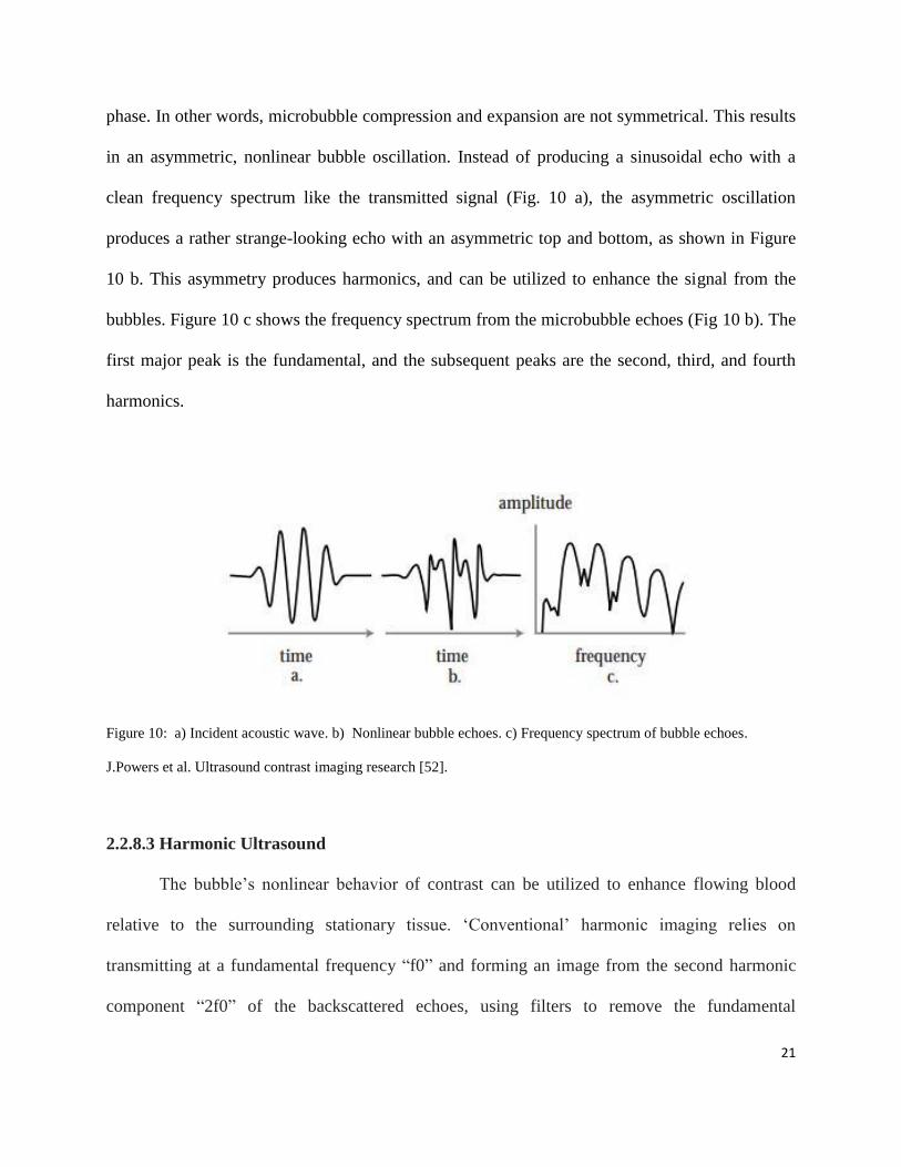
An acoustic wave generated by an ultrasound system consists of alternating high and low
pressures at frequencies of 1.5–10 MHz. When an acoustic wave encounters a microbubble, it
alternately compresses the microbubble in the positive pressure phase, and expands it in the
negative pressure phase. However, the extent to which the bubbles are compressed during the
positive pressure phase does not correspond to the extent of expansion in the negative pressure
21
phase. In other words, microbubble compression and expansion are not symmetrical. This results
in an asymmetric, nonlinear bubble oscillation. Instead of producing a sinusoidal echo with a
clean frequency spectrum like the transmitted signal (Fig. 10 a), the asymmetric oscillation
produces a rather strange-looking echo with an asymmetric top and bottom, as shown in Figure
10 b. This asymmetry produces harmonics, and can be utilized to enhance the signal from the
bubbles. Figure 10 c shows the frequency spectrum from the microbubble echoes (Fig 10 b). The
first major peak is the fundamental, and the subsequent peaks are the second, third, and fourth
harmonics.
Figure 10: a) Incident acoustic wave. b) Nonlinear bubble echoes. c) Frequency spectrum of bubble echoes.
J.Powers et al. Ultrasound contrast imaging research [52].
2.2.8.3 Harmonic Ultrasound
The bubble‟s nonlinear behavior of contrast can be utilized to enhance flowing blood
relative to the surrounding stationary tissue. „Conventional‟ harmonic imaging relies on
transmitting at a fundamental frequency “f0” and forming an image from the second harmonic
component “2f0” of the backscattered echoes, using filters to remove the fundamental
22
component. While effective, this restricts the bandwidth available for imaging, in order to make
sure that the received harmonic signal can be separated from the fundamental signal.
If the bandwidth of the fundamental signal overlaps that of the second harmonic, they
cannot be completely separated in the receive process. Thus, in harmonic imaging a narrower
transmit bandwidth is used.
The contrast agent is seen much more clearly in the harmonic image, allowing delineation
of the borders of the target tissue. This is very useful for echocardiographic examinations of
technically challenging patients in whom it is difficult to obtain diagnostically adequate images
of the endocardium. Originally, it was believed that harmonic imaging would allow complete
separation of signal produced by contrast agents from tissue signal, as it was assumed that the
tissue response was linear. While it has long been known that tissue does produce some
nonlinear energy, it was believed that the higher frequency harmonics produced in the tissues
would be eliminated because of their attenuation. However, it was soon found that tissue
produced significant harmonic energy, and that the high sensitivity and bandwidth of modern
ultrasound equipment could detect it. In fact, the harmonic image produced by tissue alone has
advantages, such as reduced clutter in the image and improved resolution [17, 18].
Harmonic ultrasound is a technique based on the principle of transmitting at frequency f
and receiving at frequency 2f (or 1/2f). This technology has become available through the
development of wide- bandwidth transducers. Microbubble contrast media produce a large
amount of harmonic signal. Contrast harmonic ultrasound provides the opportunity to image
patterns of high flow vasculature and overall perfusion. Regions of poor perfusion, including
necrosis or infarction, can be identified with contrast harmonic ultrasound by the absence of
flow. While proportionately lower, tissues also produce harmonic signals. Tissue harmonic
23
ultrasound sequences often improve subjective image quality compared to fundamental
ultrasound in echocardiographic and abdominal examinations [59].
2.2.8.4 Pulse Inversion Harmonic Imaging
As mentioned, harmonic imaging uses relatively narrow bandwidths to prevent
fundamental and harmonic component overlap. Pulse Inversion Harmonic (PIH) imaging avoids
these bandwidth limitations by subtracting the fundamental, rather than filtering it out [22]. Thus,
PIH imaging can separate the fundamental component of the bubble echoes from the harmonic
even when they overlap. This allows the use of broader transmit and receive bandwidths,
providing improved resolution and increased sensitivity to contrast agents. In Pulse Inversion
Harmonic imaging two pulses are transmitted down each ray line, rather than the single pulse
used in conventional harmonic or fundamental imaging. The first is a normal pulse, but the
second is an inverted replica of the first, so that wherever there is a positive pressure on the first
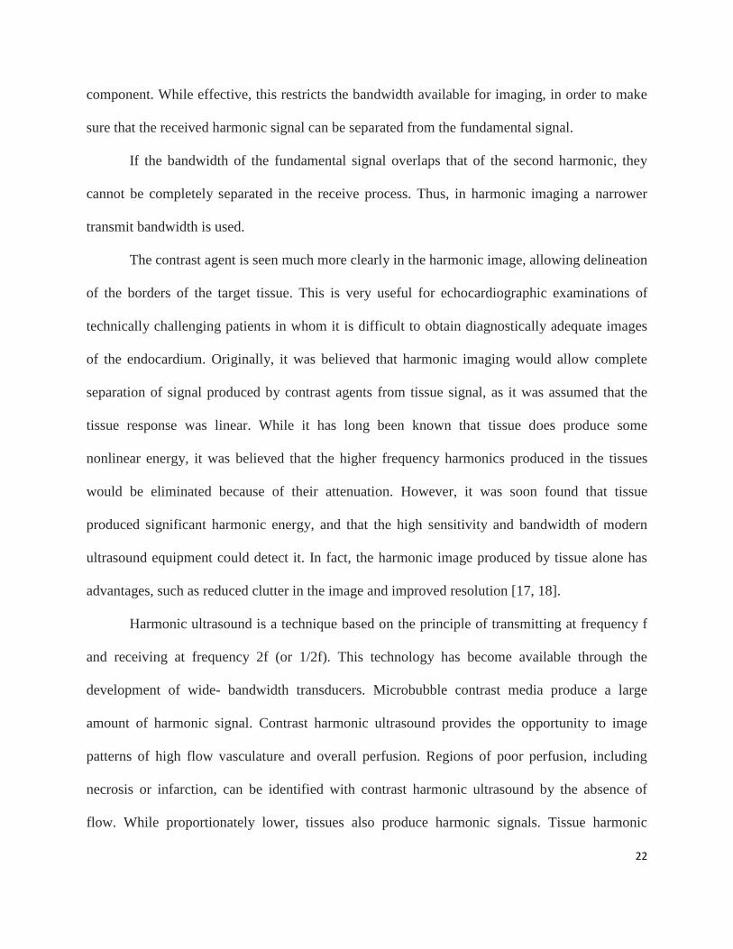
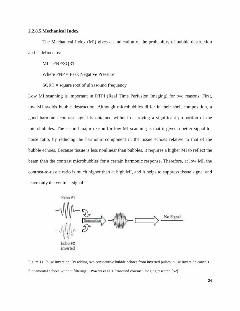
pulse there is an equal negative pressure on the second. Any linear target that responds equally to
positive and negative pressures will reflect equal but opposite echoes back to the transducer.
These echoes are then added in the beam and all stationary linear targets cancel out (fig 11). As
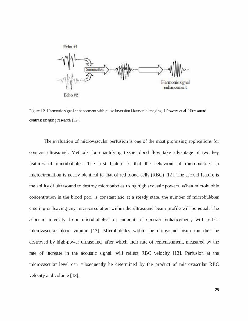
shown in Figure 13, microbubbles respond differently to positive and negative pressures and do
not reflect identical inverted waveforms. Echo #1 is identical to that shown in Figure 10 c. Echo
#2 is from the same bubble when interrogated with an inverted pulse. When these echoes are
added, they do not cancel completely. The fundamental component of the echo cancels, but the
harmonic component is added, giving twice the harmonic level of a single echo [52].
24
2.2.8.5 Mechanical Index
The Mechanical Index (MI) gives an indication of the probability of bubble destruction
and is defined as:
MI = PNP/SQRT
Where PNP = Peak Negative Pressure
SQRT = square root of ultrasound frequency
Low MI scanning is important in RTPI (Real Time Perfusion Imaging) for two reasons. First,
low MI avoids bubble destruction. Although microbubbles differ in their shell composition, a
good harmonic contrast signal is obtained without destroying a significant proportion of the
microbubbles. The second major reason for low MI scanning is that it gives a better signal-to-
noise ratio, by reducing the harmonic component in the tissue echoes relative to that of the
bubble echoes. Because tissue is less nonlinear than bubbles, it requires a higher MI to reflect the
beam than the contrast microbubbles for a certain harmonic response. Therefore, at low MI, the
contrast-to-tissue ratio is much higher than at high MI, and it helps to suppress tissue signal and
leave only the contrast signal.
Figure 11. Pulse inversion. By adding two consecutive bubble echoes from inverted pulses, pulse inversion cancels
fundamental echoes without filtering. J.Powers et al. Ultrasound contrast imaging research [52].
25
Figure 12. Harmonic signal enhancement with pulse inversion Harmonic imaging. J.Powers et al. Ultrasound
contrast imaging research [52].
The evaluation of microvascular perfusion is one of the most promising applications for
contrast ultrasound. Methods for quantifying tissue blood flow take advantage of two key
features of microbubbles. The first feature is that the behaviour of microbubbles in
microcirculation is nearly identical to that of red blood cells (RBC) [12]. The second feature is
the ability of ultrasound to destroy microbubbles using high acoustic powers. When microbubble
concentration in the blood pool is constant and at a steady state, the number of microbubbles
entering or leaving any microcirculation within the ultrasound beam profile will be equal. The
acoustic intensity from microbubbles, or amount of contrast enhancement, will reflect
microvascular blood volume [13]. Microbubbles within the ultrasound beam can then be
destroyed by high-power ultrasound, after which their rate of replenishment, measured by the
rate of increase in the acoustic signal, will reflect RBC velocity [13]. Perfusion at the
microvascular level can subsequently be determined by the product of microvascular RBC
velocity and volume [13].
26
2.2.8.6 Applications
Contrast-enhanced ultrasound (CEUS) represents a significant advancement in the
evaluation of angiogenesis in cancers. In particular, in the study of focal liver lesions, CEUS has
been widely used for detection and characterization of malignancy. The unique feature of
CEUS for non-invasive assessment of real-time liver perfusion throughout the vascular phases
has led to a great improvement in diagnostic accuracy of ultrasound, but also in guidance and
evaluation of responses to therapy. Currently, CEUS is part of the state-of-the-art diagnostic
work-up of focal liver lesions, resulting in safe and cost-effective patient management [20].
At present, improved visualization of cardiac chambers during ultrasound of the heart
(echocardiography) is the most common reason for non-microvascular blood-pool enhancement
with microbubbles. Despite advances in ultrasound imaging technology, adequate visualization
of the endocardial contours is not possible in 10-15% of patients, because of anatomical and
situational factors. Left ventricular opacification with microbubbles improves visualization of the
endocardial border, thereby increasing the accuracy of echocardiography in assessing left
ventricular size and systolic performance at rest or during stress [6], [7]. Contrast enhancement
during echocardiography can also be useful for identifying the presence of mural thrombus, left
ventricular pseudoaneurysms, and aortic dissections. More recently, CEUS has been used to
more clearly define the severity and morphological characteristics of the carotid artery [10].
Microbubbles greatly enhance Doppler signals because their backscatter is a more diffuse
reflection than from red blood cells. Microbubbles can thereby improve the accuracy of Doppler-
based methods to evaluate hemodynamic abnormalities, such as those arising from valve disease.
27
Microbubbles have also been used to examine the patency of portal veins or
portosystemic shunts on abdominal ultrasound [8]. Contrast enhancement outside the blood pool
has also been applied to detect abnormal flow patterns or anatomy. For example, microbubble
administration can assess fallopian tube patency and vesico-ureteral reflux on pelvic ultrasound
examination [9], [11].
In cardiovascular practice, this technique has been used in non-invasive detection of the
presence of coronary artery disease, to diagnose acute myocardial infarction, and to differentiate
viable myocardium from scar, all with high spatial resolution (National Cancer Institute).
Although methods for assessing perfusion were originally described for the myocardium, this
technique has been applied to assess perfusion in other organs such as the kidney, brain, skeletal
muscle and in skin grafts. Perfusion imaging with CEUS provides unique information on
microvascular blood volume and velocity not afforded by other imaging techniques, such as
MRI, radionuclide imaging, or CT. As capillaries comprises approximately 80% of the total
myocardial blood volume at rest [30], myocardial contrast echocardiography provides
information on perfusion largely at the capillary level.
The ability to characterize microvascular perfusion with microbubbles has grown
considerably since 1960s, and accounts for the majority of contrast-enhanced ultrasound studies
in some countries [60, 61]. Tumor angiogenesis results in abnormal vascular hierarchies in terms
of relative vessel size and volumetric flow. The ability to assess microvascular blood volume and
velocity separately with CEUS shows great promise for the diagnosis of primary tumors and
metastasis, and possibly for guiding new anti-angiogenic tumoricidal therapies. Contrast
ultrasound can be used to detect the abnormally high microvascular blood volume associated
with angiogenic vessels, or to detect abnormally low microvascular velocities that occur most

28
commonly in the central portions of a tumor. Contrast-enhanced ultrasound has been particularly
useful for evaluating liver masses. The relative intensity during the hepatic artery phase, the
portal venous phase, and the late or Kuppfer-cell-uptake phase has been very useful for
differentiating primary hepatic neoplasms, metastases, and haemangiomas [31].
3. Ultrasound Contrast Agents
Ultrasound contrast agents that are commonly used include particles knows as
nanoparticles that are mainly liquid or solid based. Solid and liquid nanoparticles are usually less
echogenic comparing to gas bubbles (microbubbles) due to their incompressibility. They also do
not show significant oscillation when they are exposed to the acoustic signals. However, they are
more stable at submicron diameters in comparison to microbubbles, and therefore have some
values in pharmacokinetic fields.
Due to their high echogenicity, microbubbles are ideal ultrasound contrast agents. Being
biocompatible, multifunctional, and economical are the other advantages of utilizing them in
ultrasound. Microbubbles are gas spheres between 0.1 and 10 µm in diameter and are much
smaller than the wavelength of diagnostic ultrasound, which is typically 100 to 1000 µm. Low
density and high compressibility of the gas core allows it to shrink and expand when they
encounter an acoustic signal. As a result, the diameter of the microbubble increases and
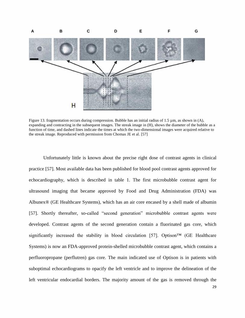
decreases rapidly giving rise to a strong and unique echo (Figure 13).
29
A B C D E F G
Figure 13. fragmentation occurs during compression. Bubble has an initial radius of 1.5 µm, as shown in (A),
expanding and contracting in the subsequent images. The streak image in (H), shows the diameter of the bubble as a
function of time, and dashed lines indicate the times at which the two-dimensional images were acquired relative to
the streak image. Reproduced with permission from Chomas JE et al. [57]
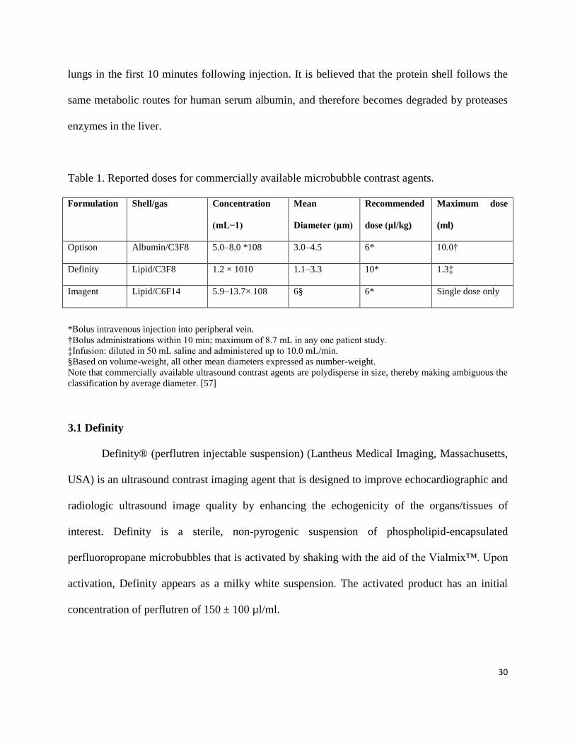
Unfortunately little is known about the precise right dose of contrast agents in clinical
practice [57]. Most available data has been published for blood pool contrast agents approved for
echocardiography, which is described in table 1. The first microbubble contrast agent for
ultrasound imaging that became approved by Food and Drug Administration (FDA) was
Albunex® (GE Healthcare Systems), which has an air core encased by a shell made of albumin
[57]. Shortly thereafter, so-called “second generation” microbubble contrast agents were
developed. Contrast agents of the second generation contain a fluorinated gas core, which
significantly increased the stability in blood circulation [57]. Optison™ (GE Healthcare
Systems) is now an FDA-approved protein-shelled microbubble contrast agent, which contains a
perfluoropropane (perflutren) gas core. The main indicated use of Optison is in patients with
suboptimal echocardiograms to opacify the left ventricle and to improve the delineation of the
left ventricular endocardial borders. The majority amount of the gas is removed through the
30
lungs in the first 10 minutes following injection. It is believed that the protein shell follows the
same metabolic routes for human serum albumin, and therefore becomes degraded by proteases
enzymes in the liver.
Table 1. Reported doses for commercially available microbubble contrast agents.
Formulation Shell/gas Concentration
(mL−1)
Mean
Diameter (μm)
Recommended
dose (μl/kg)
Maximum dose
(ml)
Optison Albumin/C3F8 5.0–8.0 *108 3.0–4.5 6* 10.0†
Definity Lipid/C3F8 1.2 × 10¹⁰ 1.1–3.3 10* 1.3‡
Imagent Lipid/C6F14 5.9–13.7× 10⁸ 6§ 6* Single dose only
*Bolus intravenous injection into peripheral vein.
†Bolus administrations within 10 min; maximum of 8.7 mL in any one patient study.
‡Infusion: diluted in 50 mL saline and administered up to 10.0 mL/min.
§Based on volume-weight, all other mean diameters expressed as number-weight.
Note that commercially available ultrasound contrast agents are polydisperse in size, thereby making ambiguous the
classification by average diameter. [57]
3.1 Definity
Definity® (perflutren injectable suspension) (Lantheus Medical Imaging, Massachusetts,
USA) is an ultrasound contrast imaging agent that is designed to improve echocardiographic and
radiologic ultrasound image quality by enhancing the echogenicity of the organs/tissues of
interest. Definity is a sterile, non-pyrogenic suspension of phospholipid-encapsulated
perfluoropropane microbubbles that is activated by shaking with the aid of the Vialmix™. Upon
activation, Definity appears as a milky white suspension. The activated product has an initial
concentration of perflutren of 150 ± 100 µl/ml.
31
Definity® was the first phospholipid-shelled, fluorocarbon/fluoropropane-gas filled agent
that received FDA approval. Gas elimination routes and shell metabolism likely are similar to
Optison. Definity was the contrast agent utilized in this study. Table 1 illustrates some data
released about characteristics and recommended dosage of microbubble contrast agents.
3.1.1 Bolus Administration
The recommended dose for Definity is a single dose of 10 µl/kg of the activated product
by intravenous bolus injection followed by saline flush. If necessary, a second 10 µl/kg dose may
be administered five minutes after the first injection to prolong contrast enhancement.
3.1.2 Infusion
Definity may also be administered via an I.V. infusion added to preservative-free saline.
The rate of infusion is suggested to be initiated at 4.0 ml/minute and could be titrated as
necessary to achieve optimal image enhancement but should not exceed 10 ml/min. The total
dose administered per kg will range from approximately 14.4 µl/kg to 21.7 µl/kg. Definity
should be used immediately after dilution with saline.
4. Tumor Vasculature
The ability of tumors to recruit blood vessels is very important to their viability, growth,
and metastasis [62]. Tumors that are smaller than 3mm can receive nutrition and oxygen from
surrounding vessels through passive diffusion [62, 63]. When tumors enlarge, they need to
overcome their nutritional needs through the proliferation of more vessels [62, 64]. This process,
which is called angiogenesis, leads tumors to have a heterogeneous texture as they grow [64, 65].
Usually, the centre of the tumor becomes hypoperfused, whereas the peripheral cells often are
32
well perfused. Multiple factors may play a role in this phenomenon, such as interstitial pressure,
variable angiogenesis in different parts of the tumor, hemorrhage, and fibrosis [62, 66]. The
assessment of tumor perfusion is very challenging, because it is a three dimensional
measurement. Measuring regional difference within a tumor is almost impossible, especially ex
vivo imaging, as an in vivo technique can depict and measure regional perfusion [62]. While
pathologists describe uniform vascular networks in a tumor, imaging studies of the same area
show regional heterogeneity. In addition, imaging evaluates patent functioning vasculature
whereas pathology determines both patent and non-patent vasculature.
5. Previous Studies
Since ultrasound contrast agents were introduced into the clinic environment, multiple
studies have evaluated its capability to improve ultrasound imaging in many organs such as the;
cardiovascular system, liver, kidneys, breasts and pancreas. There are relatively few published
articles related to the use of CEUS in the kidney.
Several studies have also been undertaken in veterinary medicine, trying to differentiate
malignant from benign tumors by evaluating different patterns of enhancement. In one of these
studies, CEUS was performed on renal tumors in 15 dogs and one cat, qualitative evaluation
showed that large tortuous arteries, early enhancement, and late wash-out were suggestive of
malignant renal tumors [67].
A 2004 study evaluated the role of CEUS in the detection of pseudocapsule in renal cell
carcinomas (RCC) in a cohort of 40 patients with biopsy proven RCC (18). Contrast-enhanced
ultrasound enabled detection of the pseudocapsule in RCC with 85.7% sensitivity [68]. A 2010
study by Zuo-Feng Xu et al. evaluated the usefulness of CEUS in differentiating RCC from renal
33
angiomyolipoma [69]. In this retrospective study, biopsy proven renal lesions underwent CEUS
to compare vascular features, such as heterogeneity, intensity of enhancement, and wash-out
speed. Contrast-enhanced ultrasound was performed after a bolus injection of Sono Vue (Bracco
SpA, Milan, Italy) and inspection of the lesion‟s vascular patterns for at least three minutes. The
sensitivity, specificity, PPV, NPV, and accuracy for characterization of RCC using CEUS
features of early wash-out, heterogeneous enhancement, and peritumoral rim enhancement were
88.2%, 97%, 98.8%, 74.4%, and 90.5% respectively, whereas homogeneous prolonged
enhancement was characteristic of angiomyolipoma. However, this study was limited as only
two different solid renal tumors were compared.
Jun Jiang et al used CEUS to assess the vascular features of clear cell RCC (CCRCC) in
this retrospective study, pathology-proven CCRCC were stratified into six groups according to
tumor size. Tumor vascular features, such as the degree of enhancement, the homogeneity of
enhancement, and the presence of a pseudocapsule, were evaluated qualitatively in six different
size groups with a 1 cm interval size difference. No relationship was found between the degree
of enhancement and tumor size. The homogeneity of tumor enhancement was reduced with
increasing lesion size, and a pseudocapsule was present in tumors between the size of 2 and 5
centimeters [70].
Pathologically proven RCC on CEUS were categorized in three groups according to the
speed of enhancement of the tumor and normal parenchymal vasculature. Considering the speed
of enhancement in the renal cortex to be normal, they categorized the enhancement speed of
tumors to three groups of early, simultaneous, and late. Xu et al. who categorized the intensity of
enhancement into three groups also adopted this approach: hypo-, iso-, and hyper-enhancement.
Heterogeneity of the tumor at CEUS was another tissue characteristic assigned a value in order
34
to differentiate tumors. Tumor wash-out speed, compared to the renal cortex, was also another
characteristic under consideration in this study. Eighty-four pathologically diagnosed RCC were
included in this retrospective study. The findings show that hyper- or iso-enhancement during the
cortical phase, a subsequent wash-out in the late phase, a heterogeneous enhancement, and a
perilesional rim-like enhancement are features that assist in characterization of RCC.
Most published CEUS studies have performed qualitative evaluation of tumor
vascularity. Commercially available software programs produced by medical imaging companies
such as Toshiba, Philips and others, have enabled real-time measurement of blood flow,
intensity, and velocity. This is done by acquiring a Time Intensity Curve (TIC) of blood flow to
measure blood volume, flow, and speed of inflow and outflow into a lesion. Quantifiable values
of these characteristics enable objective comparison between different lesions.
35
Chapter 2
Research Aims and Hypotheses
To our knowledge, our study is the first study designed to use CEUS in the evaluation of
small solid renal tumors, to characterize tumors qualitatively by analysis of their hemodynamics,
and quantitatively by measuring the Time Intensity Curve values in a large number of patients.
This study was designed to evaluate the utility of contrast enhanced contrast enhanced
ultrasound (CEUS) to differentiate between malignant and benign solid small renal masses using
both qualitative and quantitative methods. The data was kept in a locked and secured computer.
The researchers had complete control of the data and all of the information submitted for
publication. The intravenous contrast agent, Definity, supplied by the Lantheus Medical Imaging
Company (Lantheus MI Inc. Montreal, Canada) was utilized in this study.
1. Hypothesis
Evaluation of the vascular pattern and hemodynamics in solid Small Renal Masses (SRM) < 4cm
using Contrast Enhanced Ultrasound (CEUS) can differentiate malignant from benign tumors.
36
2. Objectives
2.1 Primary objective
To determine the accuracy of CEUS in differentiating malignant from benign SRM by
qualitative and quantitative evaluation of their vascular pattern and hemodynamics
2.2 Secondary objective
To evaluate the accuracy of Computed Tomography (CT) in differentiating malignant
from benign SRM by evaluation of tumor vascularity and enhancement features
37
Chapter 3
Methods
1. Study Population
1.1 Inclusion Criteria
Patients were included in the study if they had the following criteria:
18 years of age or older
Apparently solid renal lesion ≤ 4cm identified on pre-accrual CT
Tissue diagnosis based on biopsy performed pre-accrual or planned for surgery
1.2 Exclusion Criteria
Patients were excluded from the study if they had the following criteria
Refusal to consent
Pregnancy
Contraindication to the use of US contrast, such as Chronic Obstructive Pulmonary
Disease (COPD), severe heart failure (NY functional class IV)
Cystic SRM
38
1.3 Patient Population
The University Health Network Research Ethics Board approved the trial in July 2009,
and informed consent was obtained from all patients. Patients who were eligible for this study,
based on the inclusion and exclusion criteria, were informed of the study by their urologist.
Patients who showed interest in participating in the study were approached by a study
coordinator who provided them with a consent form and information about the purpose,
methods, benefits, and rare complications of the study (e.g., sensitivity to the contrast agent,
temporary headache or backache, or hypertension). Patients could withdraw from the study at
any time.
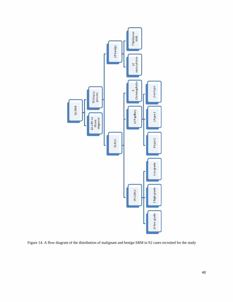
From October 2009 to September 2011, 92 patients with SRM were consented and
enrolled in this study. Twenty-two patients were subsequently excluded, since they had not
undergone tissue diagnosis by the date of data review. Therefore, the study cohort consisted of
70 patients, (44 male, 26 female) each with a single renal mass.
A flow diagram of SRM characterization by pathological type is shown in figure 14, and
tumor demographics are documented in Table 1.
The reason that only lipid-poor Angiomyolipomas (AML) were enrolled in the study was
that lipid-rich AMLs could be diagnosed accurately on CT and MRI. Lipid-poor AMLs on the
other hand do not have any characteristics to be distinguished on the current medical imaging
modalities.
39
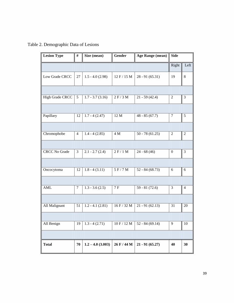
Table 2. Demographic Data of Lesions
Lesion Type # Size (mean) Gender Age Range (mean) Side
Right Left
Low Grade CRCC 27 1.5 - 4.0 (2.98) 12 F / 15 M 28 - 91 (65.31) 19 8
High Grade CRCC 5 1.7 - 3.7 (3.16) 2 F / 3 M 21 - 59 (42.4) 2 3
Papillary 12 1.7 - 4 (2.47) 12 M 48 - 85 (67.7) 7 5
Chromophobe 4 1.4 - 4 (2.85) 4 M 50 - 78 (61.25) 2 2
CRCC No Grade 3 2.1 - 2.7 (2.4) 2 F / 1 M 24 - 68 (46) 0 3
Oncocytoma 12 1.8 - 4 (3.11) 5 F / 7 M 52 - 84 (68.73) 6 6
AML 7 1.3 - 3.6 (2.5) 7 F 59 - 81 (72.6) 3 4
All Malignant 51 1.2 - 4.1 (2.81) 16 F / 32 M 21 - 91 (62.13) 31 20
All Benign 19 1.3 - 4 (2.71) 10 F / 12 M 52 - 84 (69.14) 9 10
Total 70 1.2 – 4.0 (3.003) 26 F / 44 M 21 - 91 (65.27) 40 30
40
Figure 14. A flow diagram of the distribution of malignant and benign SRM in 92 cases recruited for the study
41
Twenty-eight patients had undergone biopsy before the CEUS examination, and the
remaining 42 underwent biopsy after the CEUS. Since biopsy could influence the
hemodynamics of h of the SRMs, a minimum of six months time interval was chosen
between the biopsy and CEUS in patients in whom biopsy had been performed before
the CEUS study.
2. Ultrasound Examination
2.1 B-Mode Ultrasound
B-mode ultrasound was performed prior to CEUS in order to confirm the presence and
location of the lesion reported in previous imaging studies. A radiologist located the renal mass
on B-mode ultrasound using a PVT-375BT 3.5 MH curvilinear transducer and an Aplio XG
(Toshiba Medical Systems Corporation, Otawara-shi, Japan), documented the mass, and obtained
a video clip of the mass that could be later evaluated for several features including lesion size,
echotexture, and homogeneity.
2.2 Contrast Enhanced Ultrasound
Contrast ultrasound enhancement is defined as the appearance contrast agent in the tissue or
the field of study. Since Contrast ultrasound mode is a highly sensitive mode, it can detect just a
few bubbles.
Two commercially available US machines were used in this step of the study. A Sequoia
512 (Acuson Corporation, 1220 Charleston Road, Mountain View, Ca), considered to have the
42
best contrast resolution among the three US units, was used first following a bolus injection of
Definity to identify the lesion and acquire multiple static images and multiple Video clips for up
to 5 minutes post injection in order to review qualitative features of the mass. This study was
followed by a second bolus of contrast agent to acquire data on the IU22 (Philips Ultrasound,
Bothell WA, 98041 USA) US unit for quantitative analysis. Once the optimal approach for
viewing the kidney and lesion was determined, the data-acquisition process commenced using
low Mechanical Index (MI) nonlinear imaging in order to visualize microbubbles without
destroying them. Post-processing parameters including persistence were disabled to minimize
temporal and spatial averaging. Time-gain controls were aligned to the centerline. Receiver gain,
dynamic range, image depth, and transmit focus were optimized for each patient at the
examination.
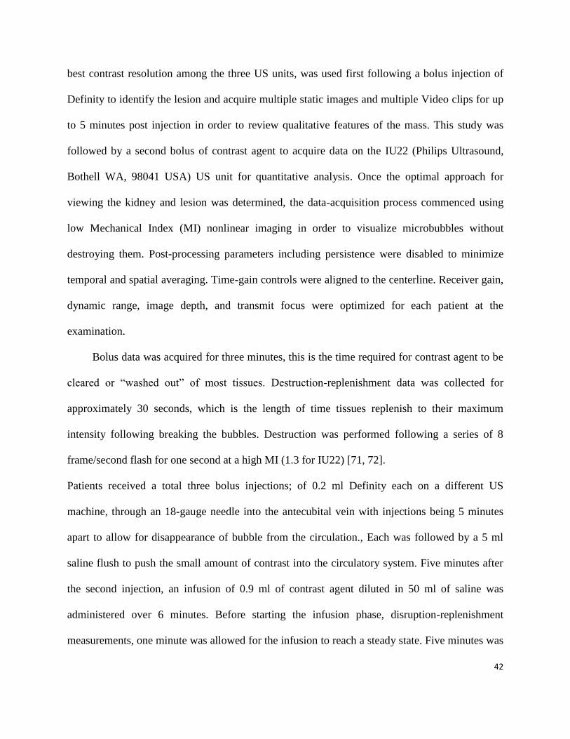
Bolus data was acquired for three minutes, this is the time required for contrast agent to be
cleared or “washed out” of most tissues. Destruction-replenishment data was collected for
approximately 30 seconds, which is the length of time tissues replenish to their maximum
intensity following breaking the bubbles. Destruction was performed following a series of 8
frame/second flash for one second at a high MI (1.3 for IU22) [71, 72].
Patients received a total three bolus injections; of 0.2 ml Definity each on a different US
machine, through an 18-gauge needle into the antecubital vein with injections being 5 minutes
apart to allow for disappearance of bubble from the circulation., Each was followed by a 5 ml
saline flush to push the small amount of contrast into the circulatory system. Five minutes after
the second injection, an infusion of 0.9 ml of contrast agent diluted in 50 ml of saline was
administered over 6 minutes. Before starting the infusion phase, disruption-replenishment
measurements, one minute was allowed for the infusion to reach a steady state. Five minutes was
43
selected as an interval time between injections to allow for most contrast agents to be removed
from blood circulation through liver or kidneys.
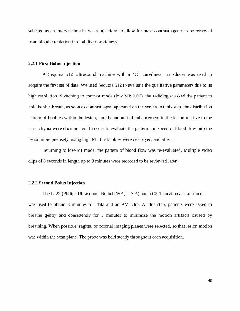
2.2.1 First Bolus Injection
A Sequoia 512 Ultrasound machine with a 4C1 curvilinear transducer was used to
acquire the first set of data. We used Sequoia 512 to evaluate the qualitative parameters due to its
high resolution. Switching to contrast mode (low MI: 0.06), the radiologist asked the patient to
hold her/his breath, as soon as contrast agent appeared on the screen. At this step, the distribution
pattern of bubbles within the lesion, and the amount of enhancement in the lesion relative to the
parenchyma were documented. In order to evaluate the pattern and speed of blood flow into the
lesion more precisely, using high MI, the bubbles were destroyed, and after
returning to low-MI mode, the pattern of blood flow was re-evaluated. Multiple video
clips of 8 seconds in length up to 3 minutes were recorded to be reviewed later.
2.2.2 Second Bolus Injection
The IU22 (Philips Ultrasound, Bothell WA, U.S.A) and a C5-1 curvilinear transducer
was used to obtain 3 minutes of data and an AVI clip. At this step, patients were asked to
breathe gently and consistently for 3 minutes to minimize the motion artifacts caused by
breathing. When possible, sagittal or coronal imaging planes were selected, so that lesion motion
was within the scan plane. The probe was held steady throughout each acquisition.

44
2.2.3 Infusion
Following the bolus injections, the remaining quantity of Definity (0.9 ml) was diluted in
50 ml of normal saline and infused into the patients‟ blood circulation during 6 minutes (three
drops/sec). After the first minute, patients were asked to hold their breath, and 30 seconds of data
was recorded on IU22 unit by destroying and replenishing Definity, using high MI. At least two
acquisitions were made. The summary of the steps and procedures can be seen on a flow diagram
provided below (Fig 15).
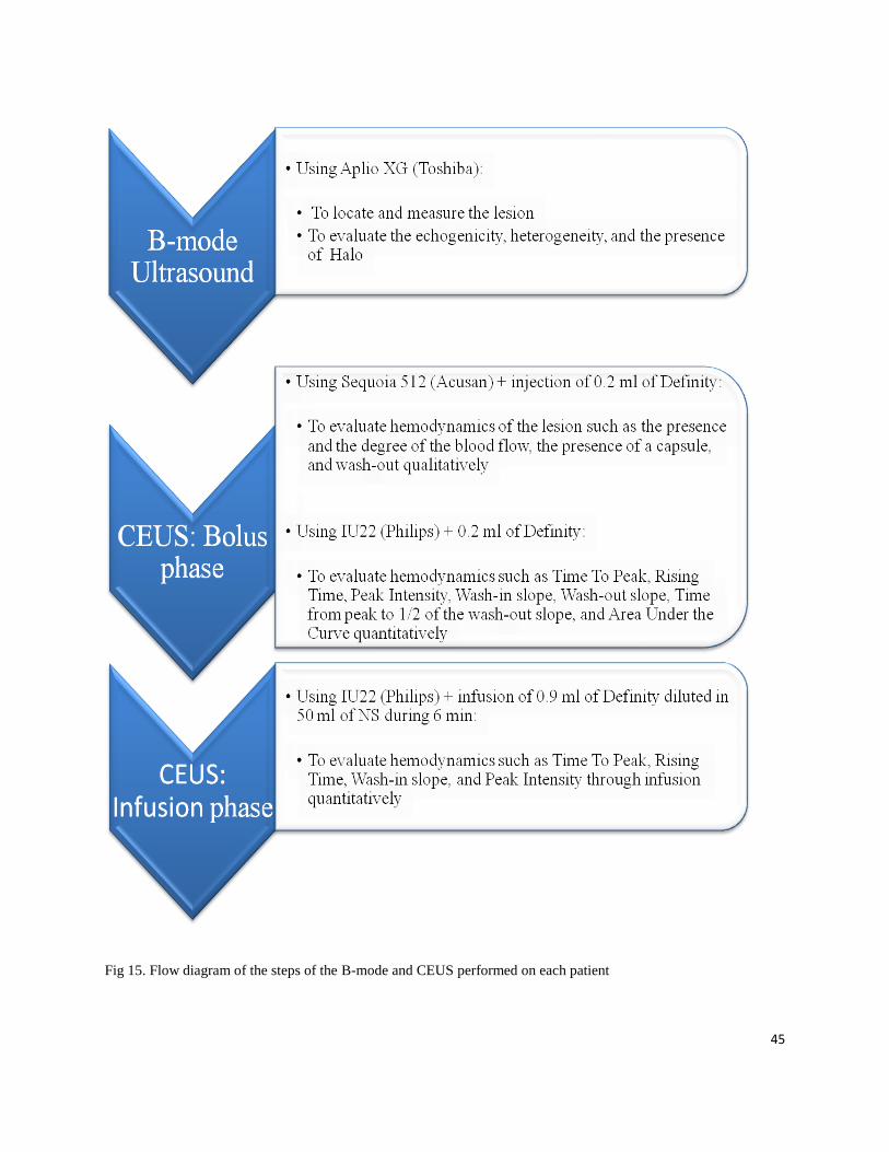
45
Fig 15. Flow diagram of the steps of the B-mode and CEUS performed on each patient
46
3. Computed Tomography (CT) examination
In order to test the secondary objective - to evaluate the accuracy of CT in differentiating
malignant from benign solid SRM by evaluation of tumour vascularity and enhancement
features, patients who had undergone multiphasic CT were enrolled in the study (63 lesions: 47
malignant, 16 benign). All cases had at least un-enhanced and Nephrographic phase helical CT,
with a 30 seconds delay for arterial phase (if there was an arterial phase), and 100 seconds delay
for Nephrographic phase. All CT examinations had a 2.5 mm slice thickness. IV contrast
Visipaue 320 was use (100 cc) for an average patient having an abdominal CT among the
remaining seven cases, two of them had undergone MRI, and five had CT with no unenhanced
phase, which could not be used in this step of our study. The research student reviewed all CT
images, and three ROIs were placed on unenhanced and Nephrographic phases of the CT
images:
The first ROI was placed on the lesion to include as much tissue of the lesion as
possible avoiding the parenchyma.
The second ROI was prescribed on the normal parenchyma of the cortex close to the
lesion (within 5 to 10 mm from the lesion).
The last ROI was placed on the normal parenchyma of the cortex as far from the
lesion as possible.
47
4. Data collection and analysis
A radiologist with 25 years of experience in ultrasound, and 6 years of experience in
contrast ultrasound collected all subjective data on grayscale US, CEUS, and CT, blinded to final
pathology.
A research student created TIC using motion compensation on QLAB software after
normalizing to the adjacent parenchyma. She also measured CT HU of unenhanced and
enhanced CT blinded to final pathology.
Acquired data was analyzed both qualitatively and quantitatively without knowledge of
the clinical history, prior imaging, and pathology result of the lesions.
SAS software 9.3 (SAS Institute INC., 100 SAS Campus Drive Cary, NC, USA), and Mann-
Whitney test were used to analyze the comparison of the quantitative parameters between
malignant and benign groups.
4.1 Qualitative Data Analysis
An abdominal radiologist with 25 years of ultrasound and 6 years of contrast US
experience reviewed all video clips recorded on the Sequoia and IU22 ultrasound machines,
independently and blinded to the final diagnosis. Sequoia clips were assessed initially followed
by IU22. Data was collected from both gray-scale and CEUS and the following features were
evaluated: for gray-scale, presence of a hypo-echoic pseudocapsule, lesion echogenicity relative
to the adjacent fat (hypo, iso, hyper), heterogeneity, and calcification, and for CEUS: vascular
pattern of enhancement, maximum degree of enhancement relative to the peak enhancement of
the adjacent cortex (hyper, iso, or hypo), heterogeneity of enhancement, presence of a vascular
pseudocapsule, and the presence of wash-out defined as more reduction of tumor enhancement as
48
compared to the adjacent cortex. The vascular pattern of enhancement was categorized as
centrifugal, centripetal, or chaotic; a centrifugal pattern is referred to a flow that proceeds in a
direction away from the centre towards the periphery, a centripetal pattern, is referred to a flow
that proceeds in a direction towards the centre, and chaotic is a pattern of flow that occurs in an
unorganized fashion.
4.2 Quantitative Data Analysis
This was performed on the data from the IU22 US units. The data was analyzed on a
commercially available software, QLAB 8.1 (Koninklijke Philips Electronics N.V. 2010).
Two regions of interest (ROI) were prescribed; one ROI was as placed on the lesion,
enclosing the largest dimension of the mass, but excluding any surrounding renal parenchyma. In
heterogeneous lesions, the ROI was placed to avoid the necrotic center and any large feeding
vessels. A second ROI was placed on the adjacent renal cortex as close to the size and depth of
the renal mass as possible. Time Intensity Curve (TIC) was obtained to document the flow of
contrast agent through the kidney and the renal mass.
4.2.1 Quantitative Analysis of Philips IU22 Data
4.2.1.1 Bolus Phase
During the three minutes data acquisition of the bolus phase, although patients were
asked to breathe as gently and consistently as possible, the movement of the abdominal organs
was inevitable. Some software programs provide an option of “motion correction” to remove the
movement effect on TIC. By activating that option, the software recognizes the speed and
49
direction of the motion. ROI placed on the tissue automatically moves with the same speed and
in the same direction to compensate the influence of movement (breathing).
On contrast mode, echo signals received by transducer are shown as brightness on the
screen of the US unit. The intensity of brightness reflects the degree of enhancement, which
itself is representative of the blood volume in a tissue. After running the acquired data in video
clip formats on the software (QLAB, Philips), and prescribing Region Of Interest (ROI) around
the lesion, the software draws a curve that illustrates the changes of brightness intensity of the
pixels inside the ROI through time. Time Intensity Curve (TIC) represents the changes of bubble
intensity (blood volume) over time.
This software provides the options for manual and automatic motion correction. We
combined both options to optimize the process by moving the ROI inside the lesion by hand, and
also by removing the frames in which the lesion and/or normal parenchyma were out of the
imaging plane, to minimize data error. To fit the raw data of TIC, QLAB 8.1 (Koninklijke
Philips Electronics N.V. 2010) provides different fitting formulas, such as the “Local Density
Random Walk” (LDRW), “Logarithmic-normal Wash-In Wash-Out” (Lognormal WI/WO), and
the “Gamma variant” formula. A literature review [73] in combination with discussion with the
manufacturer, confirmed that LDRW provides the optimal fitting-curve formula for bolus curves.
Therefore, we applied the LDRW formula to smooth our bolus TIC. Fig 16 illustrates a TIC and
its important data points.

50
Fig 16. Bolus Time Intensity Curve and its parameters
Fig 17. Infusion Time Intensity Curve and its parameters
51
4.2.1.2 Important TIC parameters [74]:
1. Wash-In slope (WI): reflects the rate of contrast agent flowing into the tissue within the
ROI, and therefore reflects the speed of blood flowing into the tissue from the point of
injection until it reaches its maximum concentration.
2. Peak Intensity (PI): is the maximum intensity value TIC within the ROI. It corresponds to
the maximum amount of microbubbles within the ROI during one passage of blood, and
is presumed to reflect the maximum tumor blood volume through that volume of tissue.
3. Time to Peak (TTP): is the time required for the contrast agent to arrive in the tumor and
reach the PI. It corresponds to the time difference between the beginning of the contrast
agent uptake and the time when the contrast agent reaches PI, another parameter that
measures the speed of inflow.
4. Rising Time (RT): A similar parameter to TTP that calculates the time taken for the
contrast to reach from 5% to 95% of the Peak /intensity (PI).
5. Wash-out slope (WO): The rate at which the tissue within the ROI empties itself of
microbubbles is shown as the Wash-out slope, and is presumed to reflect the degree of
the AV shunts inside the tumor. The higher the number of AV shunts, the steeper the
wash-out slope
6. Time from Peak to Half of the Wash-out slope (TPH1/2): Another parameter to measure
the rate at which the blood leaves the ROI, and therefore the nature of the vasculature and
the extent of shunts
7. Area under the curve (AUC): reflects the total blood volume in the tissue in 3 minutes of
data acquisition [72].
52
4.3 Additional Analysis
Besides using the fitted curve values provided by QLAB (WI slope, TTP, AUC, TPT1/2),
other parameters believed to map the important vascular behaviour of tissues were also
calculated using Mat-lab software (The Mathworks. Inc, Natick, Massachusetts, U.S.A).
1) Wash-In/Wash-Out time (WIWO-T): Measures the time that the blood takes to pass a
specific percentage of the Wash-In slope and reach the same percentage of the Wash-out
slope. For instance, 80% WIWO-T calculates the time taken for the TIC to reach from its
80% point of WI slope to its 80% of WO slope. Because blood travels through arteries to
arterioles, capillaries, venules, and veins, during this period, microbubbles might reflect
the blood flow in capillaries in both arterial and venous sides.
2) Wash-out slope at different time points: Demonstrates the down slope at different time
points after the curve reaches the peak point. Since no study has previously evaluated the
optimum time at which to calculate the WO slope, we calculated the WO slope at
different time points to determine which time point best discriminates between different
tumors.
3) Wash-out slope at different percentages of down slope: the Wash-out slopes generally
have a non-linear shape. The pattern of enhancement when normalized may behave
differently at different time points on the Wash-out slope. Considering this possibility, we
calculated the WO at different points of the slope.
5.4 Data Normalization
It was important to normalize the data from all the lesions by calculating the ratio between
measurements from the lesion and those from the adjacent normal renal cortex, since several
53
patient factors might affect the concentration, the speed of the blood flow, and thus the
enhancement of the tissue. These factors include:
1- Systemic Blood pressure
2- Atherosclerosis
3- Arterial/venous stenosis between the site of injection and the kidney
4- Low or high cardiac output
5- Cardiac shunt/valvular disease
6- Method of injection/infusion
7- Normal variants of kidney blood circulation
8- Body fat
9- US machine settings
10- Bubble destruction between site of injection and the lesion including crossing the capillary
bed in the lungs.
5.5 Statistical Analysis of Data
The data was collected on 70 patients with kidney mass that has been proved by biopsy. The
data contains qualitative variables based on the review of a radiologist and quantitative variables
based on TIC values.
The research objectives that were addressed in the statistical analysis are:
1. Descriptive statistics of qualitative variables and comparison between patients with benign
and malignant masses with regards to these variables.
54
2. Descriptive statistics of quantitative variables and comparison between patients with benign
and malignant masses in regards to these variables.
3. Sensitivity, specificity and accuracy of qualitative variables in distinguishing between type of
lesion (benign and malignant).
4. Logistic regression model to determine which variables predict type of lesion.
Categorical variables are summarized with count and percent in each category and are compared
between the two groups of patients (with benign vs. malignant masses) using the Chi-square test
for independence of two categorical variables. This test compares the distribution of the variable
of interest in the two groups. If the distributions are different the test provides statistically
significant results indicting a difference between the groups. In many cases, there were
categories with small counts, in such cases the P-values from the Fisher‟s exact test are reported.
This test is equivalent to the Chi-square but is more appropriate for small data sets.
For quantitative variables the mean, standard deviation (SD) and range are reported. A
comparison between the groups in regards to these variables was done using the Wilcoxon rank-
sum test (also known as the Mann-Whitney U test). This test is designed to make inferences
about the equality of medians of two populations based on data from independent, random
samples. This test is appropriate whenever the data is from a non-normal distribution, which is
the case in this data set.
Power calculation was done with software (PASS, version 11.0.8; NCSS, LLC). Considering
hypovascularity could differentiate between benign and malignant lesions, we divided
vascularity into two categories (hypovascular vs. isovascular or hypervascular). Based on the
55
observed data, the effect size was estimated to be 0.346. A sample size of 70 patients achieves
82% power to detect this effect size using a Chi-Square test with a significant level (alpha) of
0.05.
Statistical analyses were performed using SPSS software version 20 (IBM SSPS, Chicago,
Ill).
5.6 Student’s role in the study
The student recruited patients at kidney clinic located at Princess Margaret Hospital. She
introduced eligible cases to the attending urologist. If confirmed by the urologist, the student
explained the aim and the process of the study to the patients. She also informed them about
benefits and rare side effects of the test they were undergoing and the contrast agent that was
going to be used in the study.
Patients who were interested in participating in the study, signed an informed consent form
(ICF), and the student provided them a copy of the ICF containing all information that had been
explained to them.
The student was also in charge of arranging appointments for study cases, calling them to
confirm their participation and attendance on the arranged date and time. On the day of
examination, she explained the study steps to the patients, and helped them to get ready. In
regards to performing the test, she set up Ultrasound units and helped the radiologist acquiring
data. Other responsibility of the student was to save and keep data in a safe and locked room.
After completing each test, she placed Region Of Interest (ROI) on the renal lesion and its
adjacent cortex using Q-lab software to draw the Time Intensity Curve of each lesion and to
56
normalize it to the normal cortex of kidney. Fitting the TIC using Local Density Random Walk
method (LDRW) on Q-lab, she extracted the TIC data from Q-lab and saved it in Excel format.
In the next step she analyzed the data under supervision of a statistician.
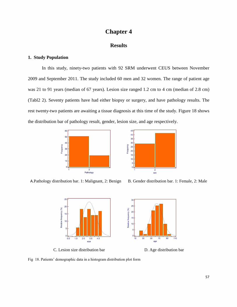
57
Chapter 4
Results
1. Study Population
In this study, ninety-two patients with 92 SRM underwent CEUS between November
2009 and September 2011. The study included 60 men and 32 women. The range of patient age
was 21 to 91 years (median of 67 years). Lesion size ranged 1.2 cm to 4 cm (median of 2.8 cm)
(Tabl2 2). Seventy patients have had either biopsy or surgery, and have pathology results. The
rest twenty-two patients are awaiting a tissue diagnosis at this time of the study. Figure 18 shows
the distribution bar of pathology result, gender, lesion size, and age respectively.
A.Pathology distribution bar. 1: Malignant, 2: Benign B. Gender distribution bar. 1: Female, 2: Male
C. Lesion size distribution bar D. Age distribution bar
Fig 18. Patients‟ demographic data in a histogram distribution plot form
58
2. Qualitative Variables: Descriptive Statistics and Comparison between Groups
For this part of the study, enhancement of solid SRMs is evaluated on CT and CEUS.
Then qualitative parameters such as Echotexture, presence of halo, heterogeneity in B-mode
ultrasound (Ultrasound without contrast) are compared between malignant and benign SRMs.
For the next step, we compared most important qualitative parameters of tumors on CEUS mode
(vascularity, enhancement pattern, presence of post-contrast halo, wash-out/retention of contrast,
and heterogeneity of enhancement) between two groups.
2.1 Enhancement of solid SRM on CT and CEUS
Considering some discrepancies between CT and CEUS in distinguishing Solid SRMs in
previous studies [75], we compared the sensitivity of CT and CEUS in confirming the solid
nature of SRMs by discerning the blood flow in tumors. While all solid SRM showed
enhancement (blood flow) on CEUS (70/70), CT failed to show vascularity in some SRMs using
HU threshold increase accepted in the literature. Considering different HU (15 and 20) as
enhancement threshold on CT to diagnose a solid mass, some of the solid SRMs did not achieve
the minimum enhancement to be considered solid SRM on CT. Table 3 illustrates the percentage
of SRM enhanced on CT and CEUS.
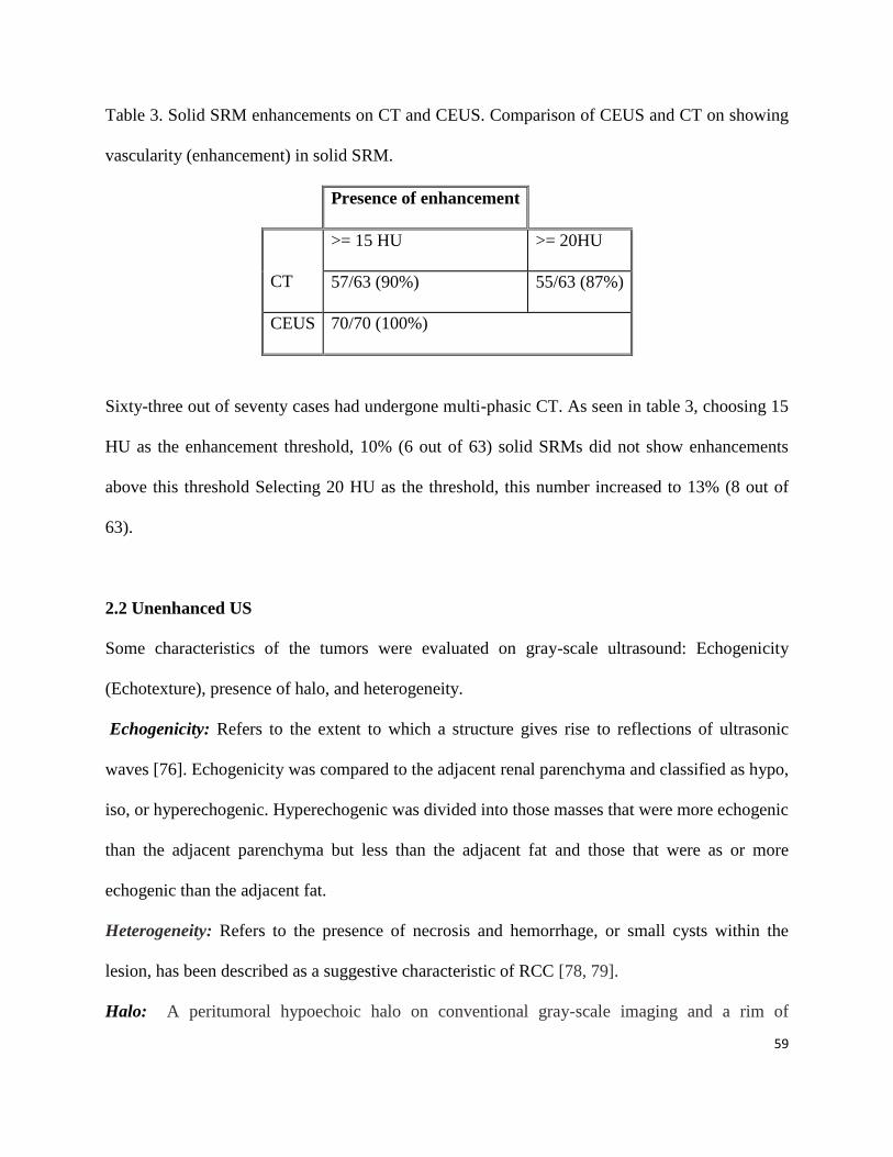
59
Table 3. Solid SRM enhancements on CT and CEUS. Comparison of CEUS and CT on showing
vascularity (enhancement) in solid SRM.
Presence of enhancement
CT
>= 15 HU >= 20HU
57/63 (90%) 55/63 (87%)
CEUS 70/70 (100%)
Sixty-three out of seventy cases had undergone multi-phasic CT. As seen in table 3, choosing 15
HU as the enhancement threshold, 10% (6 out of 63) solid SRMs did not show enhancements
above this threshold Selecting 20 HU as the threshold, this number increased to 13% (8 out of
63).
2.2 Unenhanced US
Some characteristics of the tumors were evaluated on gray-scale ultrasound: Echogenicity
(Echotexture), presence of halo, and heterogeneity.
Echogenicity: Refers to the extent to which a structure gives rise to reflections of ultrasonic
waves [76]. Echogenicity was compared to the adjacent renal parenchyma and classified as hypo,
iso, or hyperechogenic. Hyperechogenic was divided into those masses that were more echogenic
than the adjacent parenchyma but less than the adjacent fat and those that were as or more
echogenic than the adjacent fat.
Heterogeneity: Refers to the presence of necrosis and hemorrhage, or small cysts within the
lesion, has been described as a suggestive characteristic of RCC [78, 79].
Halo: A peritumoral hypoechoic halo on conventional gray-scale imaging and a rim of
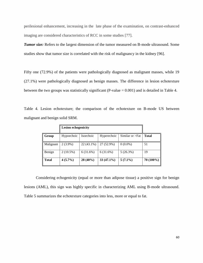
60
perilesional enhancement, increasing in the late phase of the examination, on contrast-enhanced
imaging are considered characteristics of RCC in some studies [77].
Tumor size: Refers to the largest dimension of the tumor measured on B-mode ultrasound. Some
studies show that tumor size is correlated with the risk of malignancy in the kidney [96].
Fifty one (72.9%) of the patients were pathologically diagnosed as malignant masses, while 19
(27.1%) were pathologically diagnosed as benign masses. The difference in lesion echotexture
between the two groups was statistically significant (P-value = 0.001) and is detailed in Table 4.
Table 4. Lesion echotexture; the comparison of the echotexture on B-mode US between
malignant and benign solid SRM.
Lesion echogenicity
Group Hypoechoic Isoechoic Hyperechoic Similar or >Fat Total
Malignant 2 (3.9%) 22 (43.1%) 27 (52.9%) 0 (0.0%) 51
Benign 2 (10.5%) 6 (31.6%) 6 (31.6%) 5 (26.3%) 19
Total 4 (5.7%) 28 (40%) 33 (47.1%) 5 (7.1%) 70 (100%)
Considering echogenicity (equal or more than adipose tissue) a positive sign for benign
lesions (AML), this sign was highly specific in characterizing AML using B-mode ultrasound.
Table 5 summarizes the echotexture categories into less, more or equal to fat.
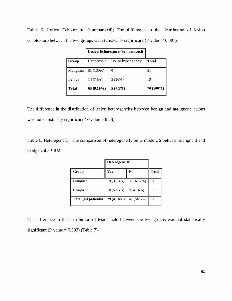
61
Table 5. Lesion Echotexture (summarized); The difference in the distribution of lesion
echotexture between the two groups was statistically significant (P-value < 0.001).
Lesion Echotexture (summarized)
Group Hypoechoic Iso- or hyper-echoic Total
Malignant 51 (100%) 0 51
Benign 14 (74%) 5 (26%) 19
Total 65 (92.9%) 5 (7.1%) 70 (100%)
The difference in the distribution of lesion heterogeneity between benign and malignant lesions
was not statistically significant (P-value = 0.28)
Table 6. Heterogeneity. The comparison of heterogeneity on B-mode US between malignant and
benign solid SRM.
Heterogeneity
Group Yes No Total
Malignant 19 (37.3%) 32 (62.7%) 51
Benign 10 (52.6%) 9 (47.4%) 19
Total (all patients) 29 (41.4%) 41 (58.6%) 70
The difference in the distribution of lesion halo between the two groups was not statistically
significant (P-value = 0.303) (Table 7).
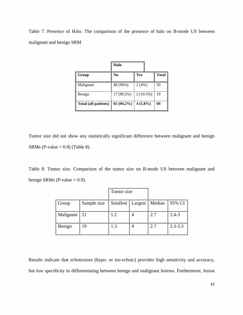
62
Table 7. Presence of Halo. The comparison of the presence of halo on B-mode US between
malignant and benign SRM
Halo
Group No Yes Total
Malignant 48 (96%) 2 (4%) 50
Benign 17 (89.5%) 2 (10.5%) 19
Total (all patients) 65 (94.2%) 4 (5.8%) 69
Tumor size did not show any statistically significant difference between malignant and benign
SRMs (P-value = 0.9) (Table 8).
Table 8. Tumor size. Comparison of the tumor size on B-mode US between malignant and
benign SRMs (P-value = 0.9).
Tumor size
Group Sample size Smallest Largest Median 95% CI
Malignant 51 1.2 4 2.7 2.4-3
Benign 19 1.3 4 2.7 2.3-3.3
Results indicate that echotexture (hypo- or iso-echoic) provides high sensitivity and accuracy,
but low specificity in differentiating between benign and malignant lesions. Furthermore, lesion

63
heterogeneity provides low sensitivity, specificity, and accuracy, and presence of a halo provides
vary low sensitivity and low accuracy but relatively high specificity in differentiating between
benign and malignant lesions (Table 9).
Table 9. Ultrasound features. Summary of in comparison of malignant to benign solid SRM on
B-mode US.
Variable
Sensitivity
(95% CI)
Specificity
(95% CI)
PPV
(95% CI)
NPV
(95% CI)
Accuracy
(95% CI)
P-
value
s
Echogenicity in favor of
benign SRM
26% 100% 100% 78% 76.00%
<0.00
1
(9-51%) (94-100%) (67-88%) (55–100%) (65- 84%)
Heterogeneity in favor of
malignancy
37% 47% 66% 22 % 40.00% 0.28
(24.13 -
51.92)
(24.45 -
71.14)
(45.67 -
82.06)
(10.56 -
37.61)
(28.47 -
52.41)
Halo in favor of malignancy 4.% 89% 50.00% 26% 28% 0.3
(0.49 -
13.71)
(66.86 -
98.70)
(6.76 -
93.24)
(16.03 -
38.64)
(17.46 -
39.62)
As seen in table 8, while high echogenicity, equal or more than the adjacent fat, in B-mode was
able to distinguish benign SRMs (AMLs) with a 100% specificity and statistically significant P-
value, other B-mode features (heterogeneity and presence of hypo halo) could not differentiate
malignant from benign SRMs.
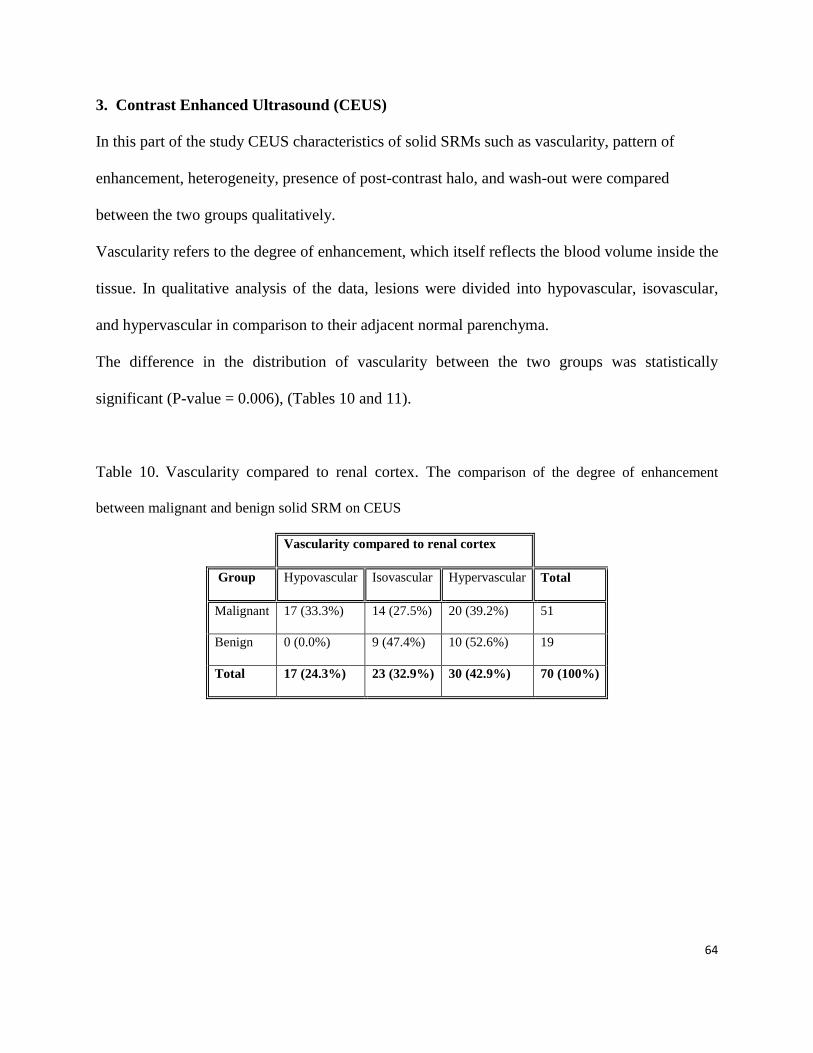
64
3. Contrast Enhanced Ultrasound (CEUS)
In this part of the study CEUS characteristics of solid SRMs such as vascularity, pattern of
enhancement, heterogeneity, presence of post-contrast halo, and wash-out were compared
between the two groups qualitatively.
Vascularity refers to the degree of enhancement, which itself reflects the blood volume inside the
tissue. In qualitative analysis of the data, lesions were divided into hypovascular, isovascular,
and hypervascular in comparison to their adjacent normal parenchyma.
The difference in the distribution of vascularity between the two groups was statistically
significant (P-value = 0.006), (Tables 10 and 11).
Table 10. Vascularity compared to renal cortex. The comparison of the degree of enhancement
between malignant and benign solid SRM on CEUS
Vascularity compared to renal cortex
Group Hypovascular Isovascular Hypervascular Total
Malignant 17 (33.3%) 14 (27.5%) 20 (39.2%) 51
Benign 0 (0.0%) 9 (47.4%) 10 (52.6%) 19
Total 17 (24.3%) 23 (32.9%) 30 (42.9%) 70 (100%)

65
Table 11. Vascularity compared to renal cortex. The comparison of the degree of enhancement
between malignant and benign solid SRM on CEUS, combining iso and hypervascular lesions into one
group
Vascularity compared to renal cortex
Group Hypovascular Iso/Hypervascular Total
Malignant 17 (33.3%) 34 (66.7%) 51
Benign 0 (0.0%) 19 (100%) 19
Total 17 (24.3%) 53 (75.7%) 70 (100%)
Combining isovascular and hypervascular, the difference is still significant (P-value = 0.003).
As seen in table 10, hypovascularity with 100% specificity is in favor of malignancy in our
study.
Figure 19. A: A papillary tumor on B-mode ultrasound. B: the same lesion with hypovascular pattern on CEUS
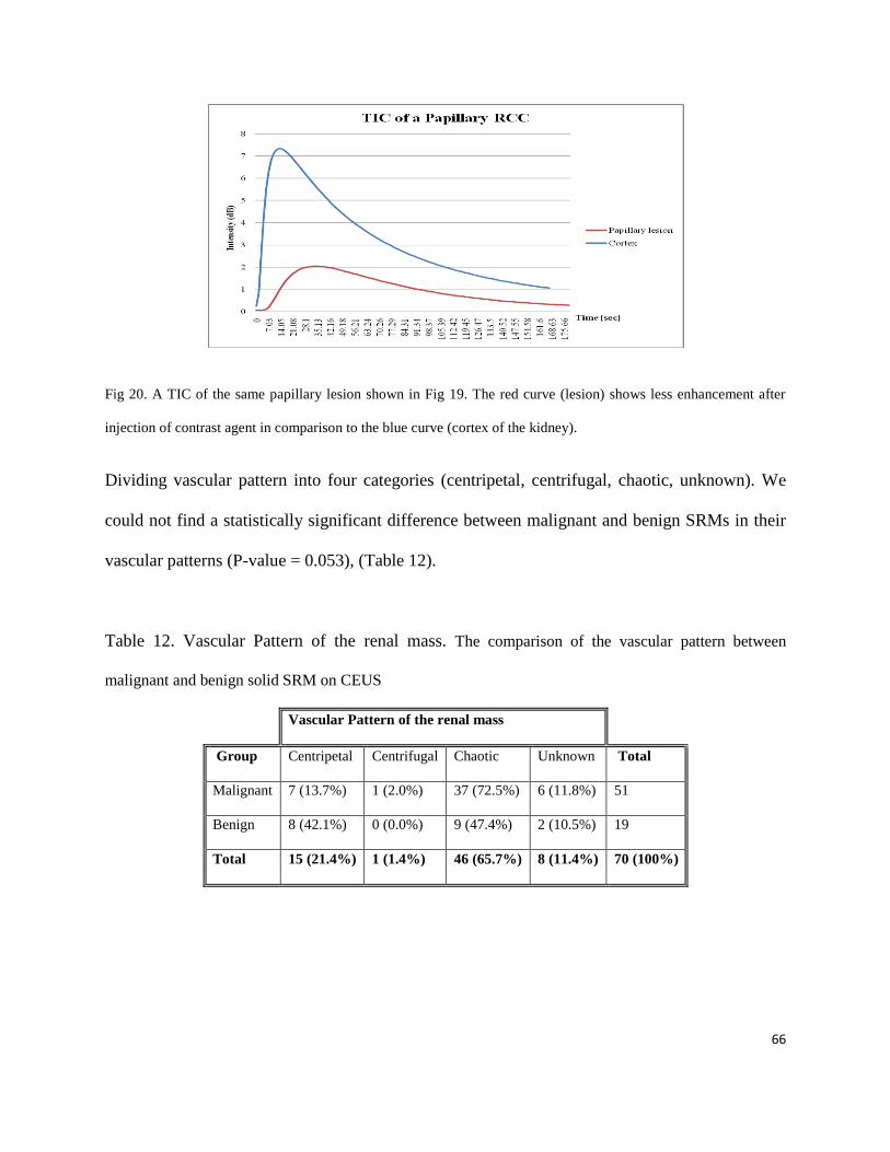
66
Fig 20. A TIC of the same papillary lesion shown in Fig 19. The red curve (lesion) shows less enhancement after
injection of contrast agent in comparison to the blue curve (cortex of the kidney).
Dividing vascular pattern into four categories (centripetal, centrifugal, chaotic, unknown). We
could not find a statistically significant difference between malignant and benign SRMs in their
vascular patterns (P-value = 0.053), (Table 12).
Table 12. Vascular Pattern of the renal mass. The comparison of the vascular pattern between
malignant and benign solid SRM on CEUS
Vascular Pattern of the renal mass
Group Centripetal Centrifugal Chaotic Unknown Total
Malignant 7 (13.7%) 1 (2.0%) 37 (72.5%) 6 (11.8%) 51
Benign 8 (42.1%) 0 (0.0%) 9 (47.4%) 2 (10.5%) 19
Total 15 (21.4%) 1 (1.4%) 46 (65.7%) 8 (11.4%) 70 (100%)
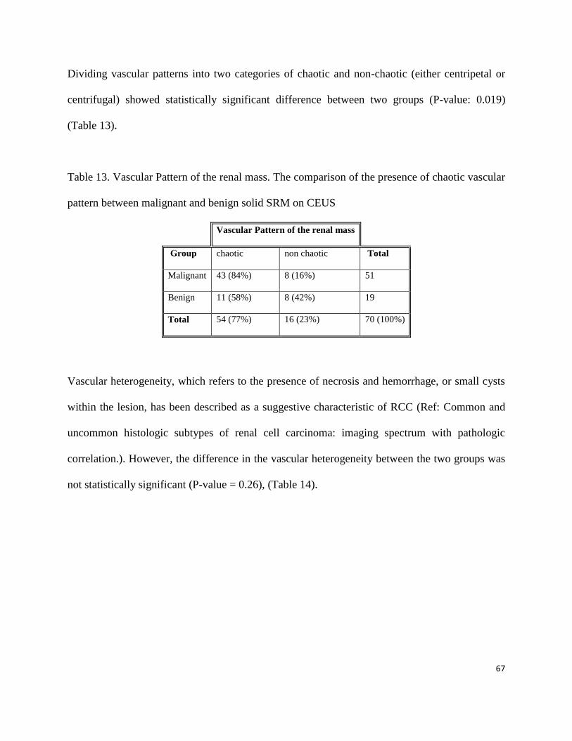
67
Dividing vascular patterns into two categories of chaotic and non-chaotic (either centripetal or
centrifugal) showed statistically significant difference between two groups (P-value: 0.019)
(Table 13).
Table 13. Vascular Pattern of the renal mass. The comparison of the presence of chaotic vascular
pattern between malignant and benign solid SRM on CEUS
Vascular Pattern of the renal mass
Group chaotic non chaotic Total
Malignant 43 (84%) 8 (16%) 51
Benign 11 (58%) 8 (42%) 19
Total 54 (77%) 16 (23%) 70 (100%)
Vascular heterogeneity, which refers to the presence of necrosis and hemorrhage, or small cysts
within the lesion, has been described as a suggestive characteristic of RCC (Ref: Common and
uncommon histologic subtypes of renal cell carcinoma: imaging spectrum with pathologic
correlation.). However, the difference in the vascular heterogeneity between the two groups was
not statistically significant (P-value = 0.26), (Table 14).
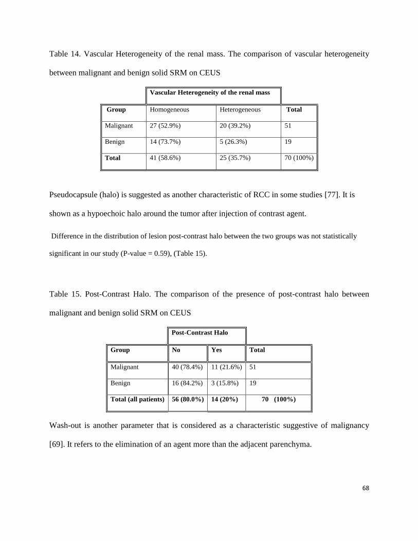
68
Table 14. Vascular Heterogeneity of the renal mass. The comparison of vascular heterogeneity
between malignant and benign solid SRM on CEUS
Vascular Heterogeneity of the renal mass
Group Homogeneous Heterogeneous Total
Malignant 27 (52.9%) 20 (39.2%) 51
Benign 14 (73.7%) 5 (26.3%) 19
Total 41 (58.6%) 25 (35.7%) 70 (100%)
Pseudocapsule (halo) is suggested as another characteristic of RCC in some studies [77]. It is
shown as a hypoechoic halo around the tumor after injection of contrast agent.
Difference in the distribution of lesion post-contrast halo between the two groups was not statistically
significant in our study (P-value = 0.59), (Table 15).
Table 15. Post-Contrast Halo. The comparison of the presence of post-contrast halo between
malignant and benign solid SRM on CEUS
Post-Contrast Halo
Group No Yes Total
Malignant 40 (78.4%) 11 (21.6%) 51
Benign 16 (84.2%) 3 (15.8%) 19
Total (all patients) 56 (80.0%) 14 (20%) 70 (100%)
Wash-out is another parameter that is considered as a characteristic suggestive of malignancy
[69]. It refers to the elimination of an agent more than the adjacent parenchyma.

69
Summarizing categories into two general classes of presence or absence of wash-out in
differentiating benign from malignant lesion, we found a higher prevalence of wash-out in
malignant lesions (P-value = 0.046), (Table 16).
Table 16. Wash-out/ Retention. The comparison of the presence of wash-out between malignant
and benign solid SRM on CEUS.
Wash-Out
Group Yes No Total
Malignant 21 (41.2%) 30 (58.8%) 51
Benign 3 (15.8%) 16 (84.2%) 19
Total 24 (34.3%) 46 (65.7%) 70 (100%)
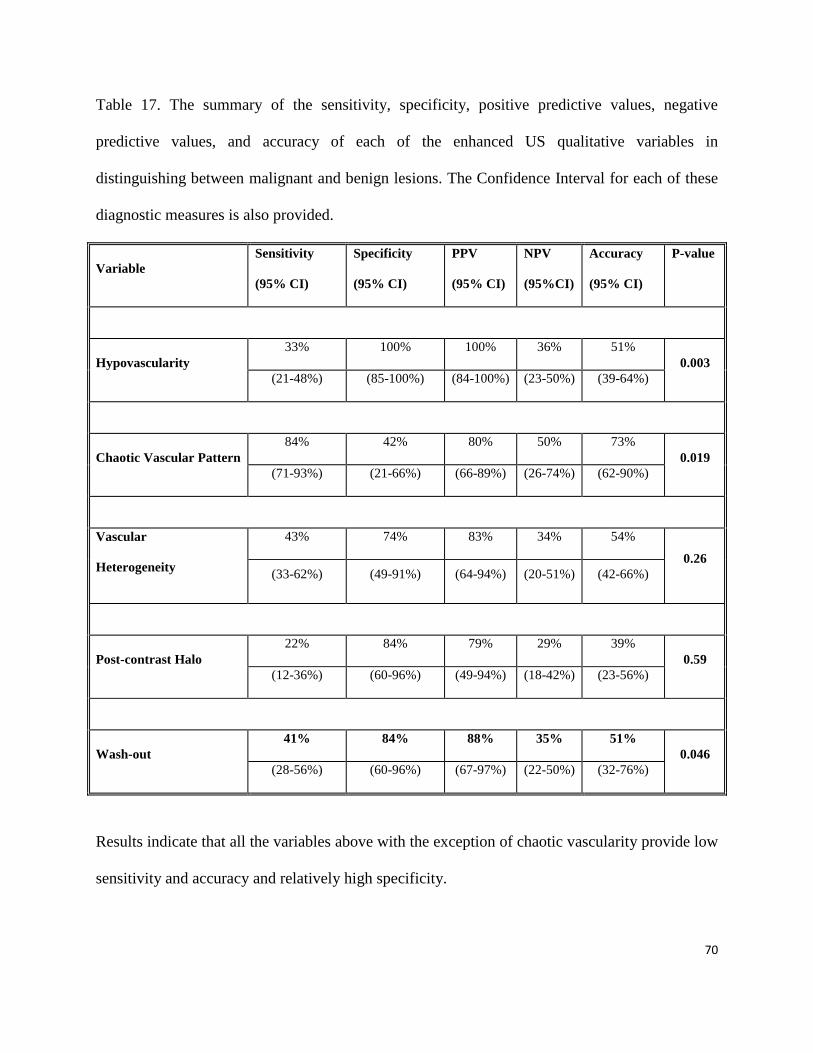
70
Table 17. The summary of the sensitivity, specificity, positive predictive values, negative
predictive values, and accuracy of each of the enhanced US qualitative variables in
distinguishing between malignant and benign lesions. The Confidence Interval for each of these
diagnostic measures is also provided.
Variable
Sensitivity
(95% CI)
Specificity
(95% CI)
PPV
(95% CI)
NPV
(95%CI)
Accuracy
(95% CI)
P-value
Hypovascularity
33% 100% 100% 36% 51%
0.003
(21-48%) (85-100%) (84-100%) (23-50%) (39-64%)
Chaotic Vascular Pattern
84% 42% 80% 50% 73%
0.019
(71-93%) (21-66%) (66-89%) (26-74%) (62-90%)
Vascular
Heterogeneity
43% 74% 83% 34% 54%
0.26
(33-62%) (49-91%) (64-94%) (20-51%) (42-66%)
Post-contrast Halo
22% 84% 79% 29% 39%
0.59
(12-36%) (60-96%) (49-94%) (18-42%) (23-56%)
Wash-out
41% 84% 88% 35% 51%
0.046
(28-56%) (60-96%) (67-97%) (22-50%) (32-76%)
Results indicate that all the variables above with the exception of chaotic vascularity provide low
sensitivity and accuracy and relatively high specificity.
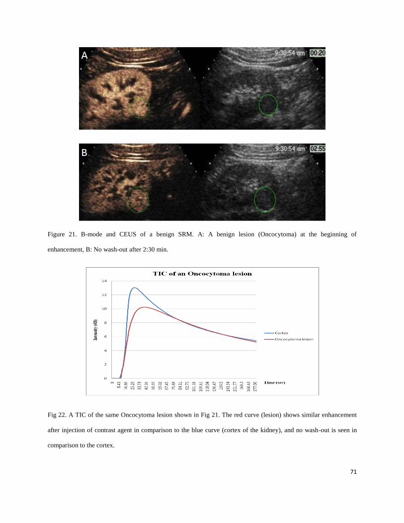
71
Figure 21. B-mode and CEUS of a benign SRM. A: A benign lesion (Oncocytoma) at the beginning of
enhancement, B: No wash-out after 2:30 min.
Fig 22. A TIC of the same Oncocytoma lesion shown in Fig 21. The red curve (lesion) shows similar enhancement
after injection of contrast agent in comparison to the blue curve (cortex of the kidney), and no wash-out is seen in
comparison to the cortex.
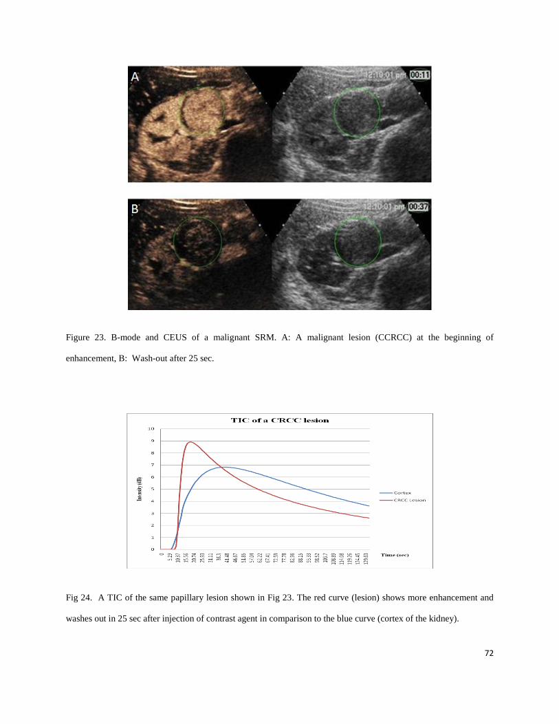
72
Figure 23. B-mode and CEUS of a malignant SRM. A: A malignant lesion (CCRCC) at the beginning of
enhancement, B: Wash-out after 25 sec.
Fig 24. A TIC of the same papillary lesion shown in Fig 23. The red curve (lesion) shows more enhancement and
washes out in 25 sec after injection of contrast agent in comparison to the blue curve (cortex of the kidney).
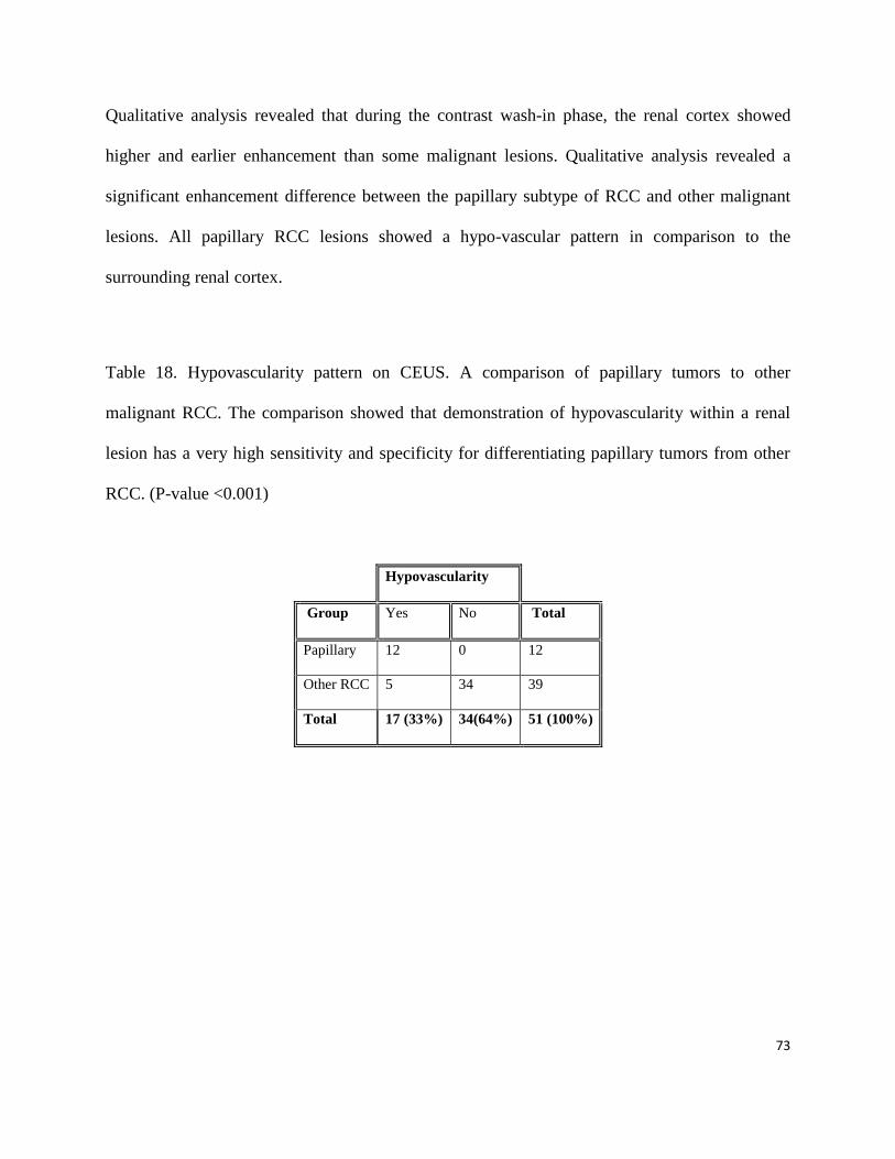
73
Qualitative analysis revealed that during the contrast wash-in phase, the renal cortex showed
higher and earlier enhancement than some malignant lesions. Qualitative analysis revealed a
significant enhancement difference between the papillary subtype of RCC and other malignant
lesions. All papillary RCC lesions showed a hypo-vascular pattern in comparison to the
surrounding renal cortex.
Table 18. Hypovascularity pattern on CEUS. A comparison of papillary tumors to other
malignant RCC. The comparison showed that demonstration of hypovascularity within a renal
lesion has a very high sensitivity and specificity for differentiating papillary tumors from other
RCC. (P-value <0.001)
Hypovascularity
Group Yes No Total
Papillary 12 0 12
Other RCC 5 34 39
Total 17 (33%) 34(64%) 51 (100%)
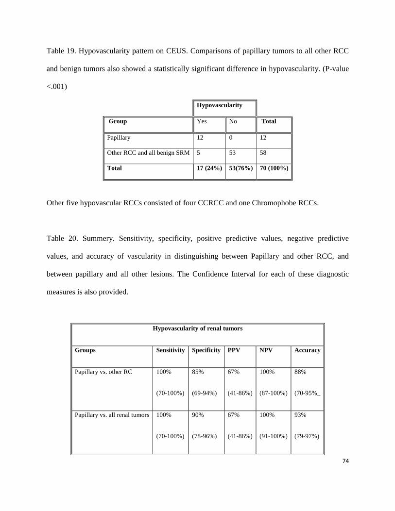
74
Table 19. Hypovascularity pattern on CEUS. Comparisons of papillary tumors to all other RCC
and benign tumors also showed a statistically significant difference in hypovascularity. (P-value
<.001)
Hypovascularity
Group Yes No Total
Papillary 12 0 12
Other RCC and all benign SRM 5 53 58
Total 17 (24%) 53(76%) 70 (100%)
Other five hypovascular RCCs consisted of four CCRCC and one Chromophobe RCCs.
Table 20. Summery. Sensitivity, specificity, positive predictive values, negative predictive
values, and accuracy of vascularity in distinguishing between Papillary and other RCC, and
between papillary and all other lesions. The Confidence Interval for each of these diagnostic
measures is also provided.
Hypovascularity of renal tumors
Groups Sensitivity Specificity PPV NPV Accuracy
Papillary vs. other RC 100%
(70-100%)
85%
(69-94%)
67%
(41-86%)
100%
(87-100%)
88%
(70-95%_
Papillary vs. all renal tumors 100%
(70-100%)
90%
(78-96%)
67%
(41-86%)
100%
(91-100%)
93%
(79-97%)

75
4. Quantitative Assessment of Renal Masses with QLAB
4.1 Quantitative Variables: Descriptive Statistics and Comparison between Groups
Table 21. Provides the mean, SD, and minimum and maximum for each quantitative variable, as
well as the P-Value from the comparison of the two groups. Since the quantitative data for nine
malignant tumors was truncated, these patients were excluded from the study population during
quantitative analysis, and the study cohort dropped from 51 to 42 patients.
Malignant, n = 42 Benign, n = 19
Variable Mean SD Min. Max. Mean SD Min. Max. P-Value
Peak Intensity 1.877 2.701 0.075 16.417 1.069 0.637 0.303 2.457 0.311
Wash-In Slope
5 - 45%
2.190 4.301 0.038 27.936 1.203 1.411 0.146 6.435 0.243
Wash-In Slope 10 - 90% 2.599 5.416 0.060 34.801 1.371 1.315 0.238 5.689 0.304
Wash-In Slope 50 - 100% 2.925 5.687 0.045 36.216 1.419 1.197 0.196 4.880 0.249
Wash-Out Slope
100 - 50%
2.23 1.997 0.019 8.586 4.34 8.490 0.050 27.69 0.057
Wash-Out Slope 100 - 10% 2.354 3.258 0.034 15.292 1.050 0.614 0.301 2.449 0.171
Wash-Out Intensity Peak +30s* 3.104 4.987 0.028 26.027 1.602 1.209 0.073 3.804 0.263
As seen the difference in each of the quantitative variables between the malignant and benign
groups was not statistically significant.
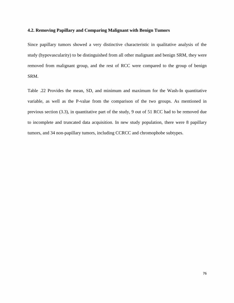
76
4.2. Removing Papillary and Comparing Malignant with Benign Tumors
Since papillary tumors showed a very distinctive characteristic in qualitative analysis of the
study (hypovascularity) to be distinguished from all other malignant and benign SRM, they were
removed from malignant group, and the rest of RCC were compared to the group of benign
SRM.
Table .22 Provides the mean, SD, and minimum and maximum for the Wash-In quantitative
variable, as well as the P-value from the comparison of the two groups. As mentioned in
previous section (3.3), in quantitative part of the study, 9 out of 51 RCC had to be removed due
to incomplete and truncated data acquisition. In new study population, there were 8 papillary
tumors, and 34 non-papillary tumors, including CCRCC and chromophobe subtypes.

77
Table 22. Quantitave positive results. TIC parameters illustrated in table below, showed
statistically significant differences between malignant and benign SRM groups.
Other Malignant, n = 34 Benign, n = 19
Variable Mean SD Min. Max. Mean SD Min. Max. P-Value
Peak Intensity 2.258 2.858 0.267 16.417 0.953 0.548 0.303 2.181 0.002
Wash-In Slope
5 - 45%
2.572 4.687 0.193 27.936 1.144 1.485 0.146 6.435 0.012
Wash-In Slope
10 - 90%
3.102 5.910 0.280 34.800 1.306 1.377 0.238 5.689 0.021
Wash-In Slope
50 - 100%
3.33 6.180 0.420 36.22 1.340 1.235 0.196 4.880 0.021
Wash-Out Slope 100 - 50% 3.431 5.111 0.265 27.69 1.233 0.857 0.279 3.560 0.008
Wash-Out Slope
100 - 10%
2.495 3.033 0.294 15.292 0.988 0.519 0.301 2.110 0.003
Wash-Out Intensity Peak
+30s
3.710 5.340 0.210 26.030 1.442 1.138 0.073 3.534 0.015
The malignant (excluding papillary) and benign lesions have significant differences in each of
the quantified variables. Other parameters (Time to Peak, Rising Time, Area Under the Curve,
WIWO Time, and Time from Peak to Half of WO) did not show any statistically significant
difference between malignant and benign SRM, including and excluding papillary subtypes.
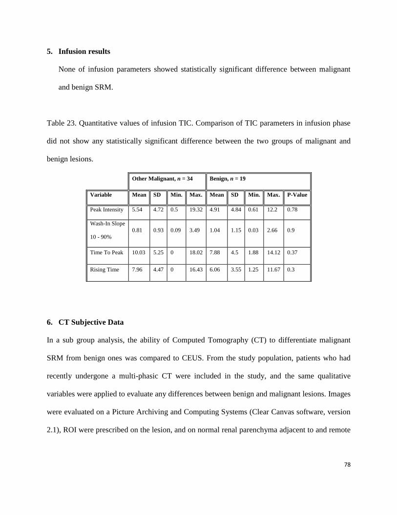
78
5. Infusion results
None of infusion parameters showed statistically significant difference between malignant
and benign SRM.
Table 23. Quantitative values of infusion TIC. Comparison of TIC parameters in infusion phase
did not show any statistically significant difference between the two groups of malignant and
benign lesions.
Other Malignant, n = 34 Benign, n = 19
Variable Mean SD Min. Max. Mean SD Min. Max. P-Value
Peak Intensity 5.54 4.72 0.5 19.32 4.91 4.84 0.61 12.2 0.78
Wash-In Slope
10 - 90%
0.81 0.93 0.09 3.49 1.04 1.15 0.03 2.66 0.9
Time To Peak 10.03 5.25 0 18.02 7.88 4.5 1.88 14.12 0.37
Rising Time 7.96 4.47 0 16.43 6.06 3.55 1.25 11.67 0.3
6. CT Subjective Data
In a sub group analysis, the ability of Computed Tomography (CT) to differentiate malignant
SRM from benign ones was compared to CEUS. From the study population, patients who had
recently undergone a multi-phasic CT were included in the study, and the same qualitative
variables were applied to evaluate any differences between benign and malignant lesions. Images
were evaluated on a Picture Archiving and Computing Systems (Clear Canvas software, version
2.1), ROI were prescribed on the lesion, and on normal renal parenchyma adjacent to and remote

79
from the lesion. Sixty-three lesions; 47/51 malignant and 16/19 benign tumors were included in
this analysis (Table 24).
Table 24. CT population. Demographic data of study population that underwent two-phasic CT
Lesion Type #
Size Range
(mean)
Gender Age Range
All Malignant 47 1.2 - 4 (2.8) 12 F / 35 M
21 - 91
(62.13)
All Benign 16 1.3 - 4 (2.7) 7 F / 9 M
52 - 84
(69.14)
Total 63 1.3 – 4 (2.9) 19 F / 44 M 21 - 91 (65.5)
There was no significant difference in the distribution of lesion heterogeneity between the two
groups (P-value = 0.17), (Table .25)
Table 25. Heterogeneity. Comparison of heterogeneity between malignant and benign SRMs on
CECT.
Heterogeneity
Group No Yes Total
Malignant 35 (74.4%) 12 (25.6 %) 47
Benign 9 (56.3%) 7 (43.7%) 16
Total 42 (66.7%) 18 (33.3%) 63
The difference in the distribution of the venous phase vascularity between the two groups was
statistically not significant (P-value = 0.717), (Table 26)
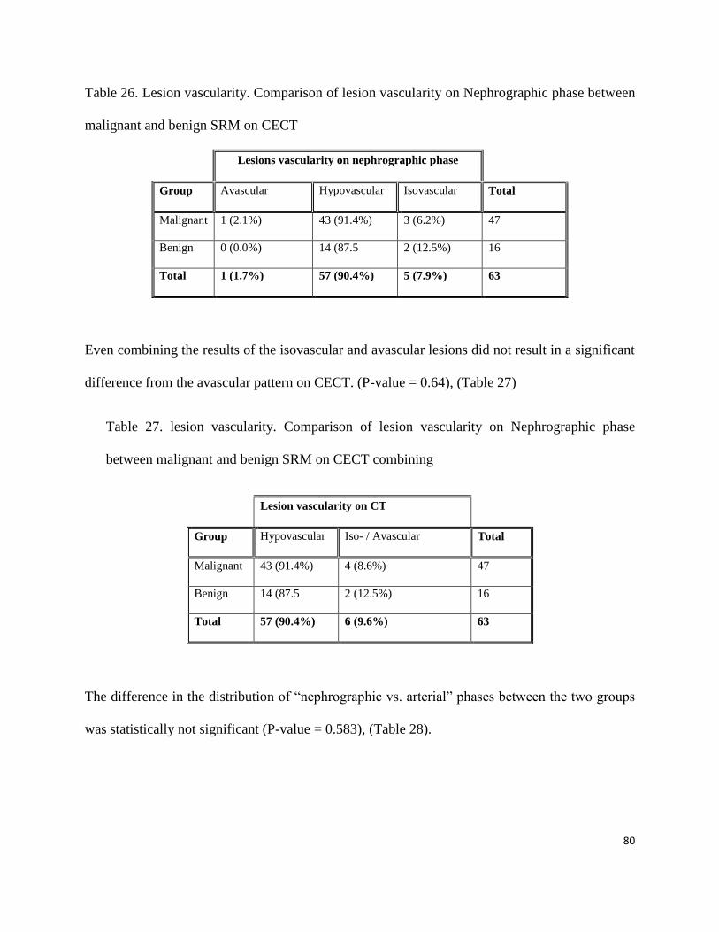
80
Table 26. Lesion vascularity. Comparison of lesion vascularity on Nephrographic phase between
malignant and benign SRM on CECT
Lesions vascularity on nephrographic phase
Group Avascular Hypovascular Isovascular Total
Malignant 1 (2.1%) 43 (91.4%) 3 (6.2%) 47
Benign 0 (0.0%) 14 (87.5 2 (12.5%) 16
Total 1 (1.7%) 57 (90.4%) 5 (7.9%) 63
Even combining the results of the isovascular and avascular lesions did not result in a significant
difference from the avascular pattern on CECT. (P-value = 0.64), (Table 27)
Table 27. lesion vascularity. Comparison of lesion vascularity on Nephrographic phase
between malignant and benign SRM on CECT combining
Lesion vascularity on CT
Group Hypovascular Iso- / Avascular Total
Malignant 43 (91.4%) 4 (8.6%) 47
Benign 14 (87.5 2 (12.5%) 16
Total 57 (90.4%) 6 (9.6%) 63
The difference in the distribution of “nephrographic vs. arterial” phases between the two groups
was statistically not significant (P-value = 0.583), (Table 28).
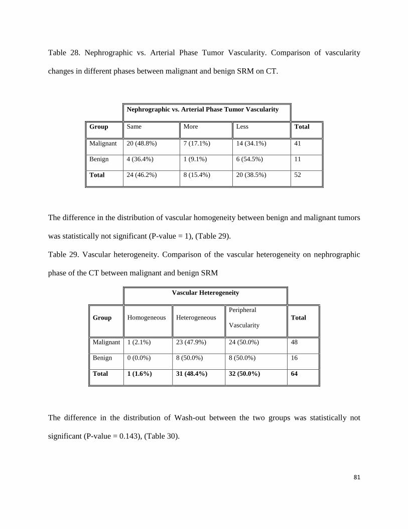
81
Table 28. Nephrographic vs. Arterial Phase Tumor Vascularity. Comparison of vascularity
changes in different phases between malignant and benign SRM on CT.
Nephrographic vs. Arterial Phase Tumor Vascularity
Group Same More Less Total
Malignant 20 (48.8%) 7 (17.1%) 14 (34.1%) 41
Benign 4 (36.4%) 1 (9.1%) 6 (54.5%) 11
Total 24 (46.2%) 8 (15.4%) 20 (38.5%) 52
The difference in the distribution of vascular homogeneity between benign and malignant tumors
was statistically not significant (P-value = 1), (Table 29).
Table 29. Vascular heterogeneity. Comparison of the vascular heterogeneity on nephrographic
phase of the CT between malignant and benign SRM
Vascular Heterogeneity
Group Homogeneous Heterogeneous
Peripheral
Vascularity Total
Malignant 1 (2.1%) 23 (47.9%) 24 (50.0%) 48
Benign 0 (0.0%) 8 (50.0%) 8 (50.0%) 16
Total 1 (1.6%) 31 (48.4%) 32 (50.0%) 64
The difference in the distribution of Wash-out between the two groups was statistically not
significant (P-value = 0.143), (Table 30).
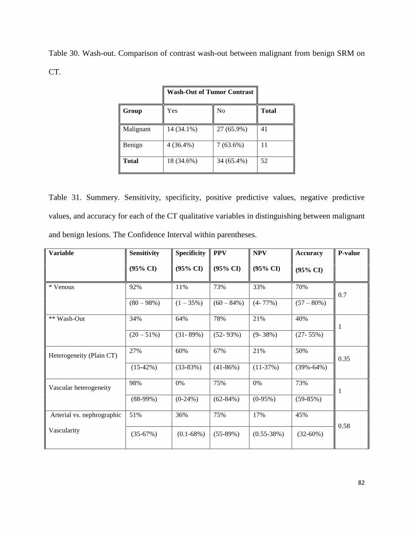
82
Table 30. Wash-out. Comparison of contrast wash-out between malignant from benign SRM on
CT.
Wash-Out of Tumor Contrast
Group Yes No Total
Malignant 14 (34.1%) 27 (65.9%) 41
Benign 4 (36.4%) 7 (63.6%) 11
Total 18 (34.6%) 34 (65.4%) 52
Table 31. Summery. Sensitivity, specificity, positive predictive values, negative predictive
values, and accuracy for each of the CT qualitative variables in distinguishing between malignant
and benign lesions. The Confidence Interval within parentheses.
Variable Sensitivity
(95% CI)
Specificity
(95% CI)
PPV
(95% CI)
NPV
(95% CI)
Accuracy P-value
(95% CI)
* Venous 92% 11% 73% 33% 70%
0.7
(80 – 98%) (1 – 35%) (60 – 84%) (4- 77%) (57 – 80%)
** Wash-Out 34% 64% 78% 21% 40%
1
(20 – 51%) (31- 89%) (52- 93%) (9- 38%) (27- 55%)
Heterogeneity (Plain CT) 27% 60% 67% 21% 50%
0.35
(15-42%) (33-83%) (41-86%) (11-37%) (39%-64%)
Vascular heterogeneity 98% 0% 75% 0% 73%
1
(88-99%) (0-24%) (62-84%) (0-95%) (59-85%)
Arterial vs. nephrographic
Vascularity
51% 36% 75% 17% 45%
0.58
(35-67%) (0.1-68%) (55-89%) (0.55-38%) (32-60%)
83
* Venous vascularity is defined as the amount of tumoral enhancement during the
nephrographic/delayed phase of CT. A minimum increase of 10 to 20 HU compared to the non-
contrast phase is considered as positive for tissue vascularity [80]. Some authors suggest that a
minimum of 20 HU increase is necessary to describe lesion enhancement with 100% specificity
[8, 81]. In this study, 20HU was used as a threshold for lesion enhancement/ wash-out.
** Wash-out is defined as a relative loss of intralesional contrast material relative to the
normal parenchyma when comparing the arterial phase to the nephrographic venous and delayed
phases has been referred to as wash-out [82]. Twenty HU was the minimum decrease of
enhancement at nephrographic phase from arterial phase to be considered wash-out in this study.
7. Logistic Regression Models
In the sections below, logistic regression models were fitted to the data. A stepwise
procedure based on likelihood ratios was used to determine which variables are significant in
predicting the type of lesion.
7.1 Wash-in Variables
Variables included in the three models below are: Peak intensity, wash-in slope 5 to 45%,
wash-in slope 10 to 90% and wash-in slope 50 to 100%.
Using the wash-in quantitative variables only to predict the type of lesion (malignant vs.
benign), none of the variables was significant.
Using the wash-in quantitative variables only to predict the type of lesion (non-papillary vs.
benign), only peak intensity was significant (P-value = 0.013). The odds of detecting a

84
malignant lesion increases by 4.45 for each increase of 1 unit in peak intensity value (95% CI
(1.363, 14.536)).
Using the wash-in quantitative variables only to predict the type of malignant lesion
(papillary versus other malignant lesions), only peak intensity was significant (P-value =
0.006). The odds of detecting other malignant lesions (non-papillary) increase by 7.35 for
each increase of 1 unit in peak intensity value (95% CI (1.788, 30.185)).
7.2 Wash-out Variables
Variables included in the three models below are: wash-out slope 100 to 50%, wash-out
slope 100 to 10% and wash-out intensity peak+30.
Using the wash-out quantitative variables only to predict the type of lesion (malignant vs.
benign), none of the variables was significant.
Using the wash-out quantitative variables only to predict the type of lesion (non-papillary vs.
benign) only 'wash-out slope 100 to 10%' was significant (P-value = 0.021). The odds of
detecting a malignant lesion increases by 5 for each increase of 1 unit in 'wash-out slope 100
to 10%' value (95% CI (1.28, 19.55)).
Using the wash-out quantitative variables only to predict the type of malignant lesion
(papillary versus other malignant) only 'wash-out slope 100 to 10%' was significant (P-value
= 0.004). The odds of detecting other malignant lesion (not papillary) increases by 22.63 for
each increase of 1 unit in 'wash-out slope 100 to 10%' value (95% CI (2.66, 192.56)).
85
7.3 Combining Wash-in and Wash-out Variables
Variables included in the three models below are: Peak intensity, wash-in slope 5 to 45%,
wash-in slope 10 to 90%, wash-in slope 50 to 100%, wash-out slope 100 to 50%, wash-out
slope 100 to 10% and wash-out intensity peak+30.
In this section, I used the 'NONTRUNC quantitative variable' excel sheet which include the
wash-in and wash-out data on 52 cases.
In a logistic regression model to predict the type of lesion (malignant vs. benign), none of the
variables was significant.
In a logistic regression model to predict the type of lesion (other malignant excluding
papillary vs. benign), only 'wash-out slope 100 to 10%' was significant (P-value = 0.021).
In a logistic regression model to predict the type of malignant lesion (papillary versus other
malignant) only 'wash-out slope 100 to 10%' was significant (P-value = 0.004).
7.4 Qualitative Variables - Unenhanced US
Variables included in the model below are echotexture, heterogeneity and halo.
None of the unenhanced US variables (echotexture, heterogeneity or halo) was significant in
predicting type of lesion (malignant vs. benign).
7.5 Qualitative Variables - Enhanced US
Variables included in the model below are: vascularity (3 categories), vascular pattern (4
categories), vascular homogeneity (3 categories), post contrast halo and wash-out (3
categories).
86
Vascularity, vascular pattern, vascular homogeneity and post contrast halo were not
significant in a logistic regression model for predicting the type of lesion (malignant vs.
benign).
Wash-out showed a trend toward being statistically significant in predicting the type of lesion
(P-value = 0.115). In particular, the odds of a case with wash-out of being malignant is
estimated to be 4.5 times the odds of a case with retention (P-value = 0.038).
7.6 Qualitative Variables - CT Data
Variables included in the model below are: CT density (4 categories), heterogeneity (2
categories), arterial vascularity cortex (4 categories), venous vascularity cortex (3
categories), portal vs. arterial, vascular homogeneity (3 categories) and wash-out (3
categories).
CT density, heterogeneity, portal vs. arterial, vascular homogeneity and wash-out were not
significant in a logistic regression model for predicting the type of lesion (malignant vs.
benign).
7.7 Qualitative Variables - Unenhanced US, Enhanced US and CT
In all the models below the same variables outlined above in each section were used, e.g., the
model for wash-in and enhanced US included all the variables listed in the wash in section
above and those listed in the enhance US above.
87
In a search for a logistic regression model for predicting the type of lesion combining
unenhanced US, enhanced US and CT variables none of the variables was significant when
combined.
7.8 Combining Qualitative and Quantitative Variables
In a search for a combination of qualitative and quantitative variables that significantly
predict the type of lesion (malignant vs. benign) in a logistic regression model the following
results were obtained.
Wash-in variables and unenhanced US - no significant combination of variables were found.
Wash-in and enhanced US - no significant combination of variables were found.
Wash-out variables and unenhanced US - no significant combination of variables were
found.
Wash-out and enhanced US - no significant combination of variables were found.
Wash-in and wash-out variables and unenhanced US - no significant combination of
variables were found.
Wash-in and wash-out and enhanced US - no significant combination of variables were
found.
All quantitative and all qualitative - no significant combination of variables were found.
88
8. Summary of the results
Ten percent of solid SRMs enhanced <15HU and 13% < 20 HU on CT, while all of them
were vascular on CEUS.
Echogenicity was in favour of benignity on B-mode ultrasound with 100% specificity.
All masses that were hypovascular vs. parenchyma were cancer with 100% specificity.
Most lesions with wash-out were cancer (84% specificity).
Chaotic vascular pattern was in favour of malignancy (Sensitivity: 84%, Specificity: 42%).
In quantitative analysis of TIC parameters, PI, Wash-in slope, Wash-out slope, and Wash-out
intensity at peak+30s were significantly higher in non-papillary cancers.
Using logistic regression model, Peak intensity and wash-out slope were significantly higher
in non-papillary malignant lesions in comparison with benign tumors
Infusion data was not significant in differentiating malignant SRMs from benign ones.
None of CT qualitative features could differentiate malignant from benign SRMs.
89
Chapter 4
Discussion
The widespread use of imaging techniques such as ultrasonography, CT, and MRI have
increased the incidental discovery of asymptomatic abdominal tumors and renal tumors in
particular during the evaluation of unrelated or nonspecific symptoms. If sufficiently large or
suspicious, these tumors may undergo biopsy or surgical removal. In other cases, imaging such
as CT and MRI are requested on a regular basis to assess any interval change in the tumor in
particular, interval growth and change in morphology. These follow up strategies are expensive
and have well defined complications such as bleeding and hematoma following biopsy, radiation
exposure and kidney dysfunction after CT, and allergic reactions to CT and MRI contrast agents.
The aim of this study was to evaluate the utility of contrast-enhanced ultrasound (CEUS) in
differentiation between benign and malignant small renal masses (SRM), in order to reduce the
number of unnecessary biopsies, surgeries or other types of management. To our knowledge, this
is the first prospective study that has evaluated both qualitative and quantitative data to
differentiate between malignant and benign SRM using CEUS.
1. Qualitative Findings
According to our findings, CEUS can play an important role in differentiating benign
from malignant solid renal masses (SRM).
90
1.1 Echo texture: Our data demonstrate that angiomyolipomas (AML) appear more
echogenic in B-mode ultrasound than malignant tumors (P-value: 0.001). An SRM
demonstrating similar or increased echo texture than the adjacent fat had 100% specificity but
only 26% sensitivity in differentiating AML from malignant lesions (PPV: 100%, NPV: 78%,
accuracy: 76%). The hyperechogenic features of the AML can be explained by the presence of
multiple fat and non-fat interfaces within the tumor [83]. Other features at B-mode ultrasound
(homogeneity and the presence of halo) did not differentiate malignant from benign lesions in
our study.
AMLs are composed of adipose tissue, smooth muscle cells, and abnormal thick-walled blood
vessels. AML represents a diagnostic challenge for every imaging method when they are of low
fat content. They may also present with hemorrhage, calcification, arteriovenous shunts (vascular
AML), and mimic malignant lesions. On US, they show a typical pronounced hyperechoic
appearance. However, iso- or hypoechoic variants are seen in 6% of cases [84]. Unenhanced CT
can diagnose the typical AML with accuracy. Up to 14% of all AML are atypical and can lead to
unnecessary surgery, especially when hemorrhage, calcification, arteriovenous shunts, necrosis
or have low fat content [84]. RCC or oncocytoma can also contain microscopic fatty components
but presence of gross fat is very rare [84].
1.2 Halo: In recent studies, the role of tumor pseudocapsule in the diagnosis of RCC is
suggested [77]. RCCs generally do not have a true histologic capsule. A pseudocapsule results
from tumor growth producing ischemia and necrosis of the adjacent normal parenchyma [77]. It
is composed of fibrous tissue and compressed renal parenchyma. This pseudocapsule is not
described in the TNM classification [77]. It is a pathologic feature frequently seen in early stage,
low-grade RCC. It is suggested as a useful sign in the differential diagnosis of RCC and in the
91
choice for a nephron sparing surgical approach. In conventional B-mode US, a pseudocapsule
appears as a peritumoral hypoechoic halo. Ascenti et al. investigated the ability of CUS to detect
a pseudocapsule in 32 patients with 40 renal masses. A pseudocapsule was correctly diagnosed
in 12/14 histologically evaluated RCC (86%). In the other renal cell carcinomas, a pseudocapsule
was not found histologically. In all other lesions, a pseudocapsule was not visible. The positive
predictive value was 100% but the negative predictive value was only 50% [77]. Jiang et al. [70]
in their study of correlating CEUS features of 92 clear cell RCC in relation to tumor size, found
out that in patients with tumors ≤ 2 cm, a pseudocapsule appeared in 3/13 cases (23%), in 38/58
cases (66%) with tumors from > 2 to 5 cm and in 5/21 cases (24%) with tumors > 5 cm.
Although most of malignant SRMs in our study were early stage and low-grade RCCs, the
majority of them were smaller than 2 cm. It is possible that lesions had not reached the size to
produce a pseudocapsule around them. The specificity of halo to predict malignancy in our study
was 89% and 4% respectively.
1.3 Heterogeneity: Renal masses appear as a homogeneous lesion on B-mode ultrasound
when they are small. As they grow, necrosis, hemorrhage, and cystic components change them to
heterogeneous lesions. Heterogeneity on B-mode ultrasound is reported in renal abscess,
pseudotumors, Wilm‟s tumor, and large tumors due to necrosis, hemorrhage, cyst, calcification
[85]. This study did not find heterogeneity in favor of malignancy. Since heterogeneity appears
to be due to rapid growth of the tumors in more malignant lesions, our negative results could be
due to small size and low grade of tumors.
1.4 Vascular enhancement: There is a significant difference between the vascular
enhancement of some malignant and benign tumors. A pattern of hypoenhancement relative to
92
the adjacent parenchyma, has 100% specificity, 33% sensitivity, 100% PPV, and 36% NPV in
certain malignant SRM that include papillary tumors, the slow-growing subtype of RCC (P-
value: 0.003) (Fig 19). When specifically comparing papillary tumors to the other malignant
renal tumors, hypovascularity showed 100% sensitivity, 85% specificity, 67% PPV, 100% NPV,
and 88% accuracy to differentiate papillary RCC from the other subtypes of RCC (P-value <
0.001). Papillary tumors also showed a statistically significant difference in hypovascularity
compared to all other lesions (P-value: <0.001, sensitivity: 100%, specificity 91%, PPV: 71%,
NPV: 100%, and accuracy: 93%). Gerst et al. in their initial experience of renal mass evaluation
with contrast ultrasound on 34 patients reported that diminished lesion enhancement relative to
parenchyma had 91% specificity, 55% sensitivity, 75% PPV and 81% NPV for non-clear cell
histological features, such as low grade malignant tumors or benign lesions (indolent tumors)
[33]. Our study did not confirm hypoenhancement as one of the characteristics of benign tumors.
None of the benign lesions in our study showed less enhancement than the renal parenchyma.
Although Gerst et al had benign lesions that demonstrated hypoenhancement, in their cohort only
one out of four benign lesions (one AML) showed hypoenhancement relative to the parenchyma,
and the other three (Oncocytomas) were iso/hyperenhancing. Some studies document hypo-
enhancement as a characteristic of AML [84], but this observation was not confirmed by our
study. This apparent contradiction can be explained by the amount of fat present in the tumor
[42]. We only enrolled lipid-poor AML in our study. Lipid-poor AML contain more vessels and
myocytes and less lipocytes, which likely explains the hyperenhancement of AML in our study.
1.5 Vascular Pattern: The chaotic vascular pattern was more commonly seen in
malignant masses (P-value: 0.019) in our series. Renal lesions are considered malignant when
vessels with an abnormal course or branching pattern are observed, and there are increased or
93
decreased vascularization compared with adjacent normal cortex [67]. Haendl in his study on
vascular pattern in RCC [86], reports chaotic vascular pattern in all RCCs but one, which was a
cystic lesion, and had no enhancement [79].
Baish and Jain also showed that malignant tumors have a much higher vascular complexity as
compared with normal vasculature [87].
1.6 Wash-out: The difference in wash-out between all malignant and all benign tumors
reached statistical significance (P-value: 0.046) (sensitivity: 41%, specificity: 84%, PPV: 88%,
NPV: 35%, accuracy: 53%). Xu et al. in their study on 126 renal masses found wash-out,
heterogeneity, and pseudo capsule in favor of RCC, and homogenous and prolonged
enhancement in the absence of pseudo capsule in his study were suggestive of benign renal mass
[69]. Huang et al in their study about the value of contrast-enhanced ultrasonography in
differentiation of subtypes of renal cell carcinoma divided vascular enhancement of renal masses
into three phases: Cortical phase, peak time phase, and parenchymal phase. They found out from
their results that the isochronous/delayed enhancements in cortical phase, hypoechoic/isoechoic
in peak time, and fast wash-out in parenchymal phase were main types in Papillary and
Chromophobe RCCs [88].
RCC is characterized by numerous thin-walled blood vessels with rich blood flow
pathologically [75, 89], and this fact may explain the other reason for wash-out.
1.7 Tumor Heterogeneity: One of the other objectives of this study was to compare the
heterogeneity of the tumors post enhancement between malignant and benign tumors. Unlike
other studies (26), this study did not show significant difference in vascular heterogeneity
between malignant and benign tumors (P-value = 0.2). Tumor heterogeneity can be explained by
the presence of necrosis and hematoma in central parts of the tumor. However, this phenomenon
94
occurs more frequently with larger tumors. The lack of a significant difference in tumor
enhancement (heterogeneity vs., homogeneity) in our cohort could be due to the small size of the
lesions in this study. Necrosis is also more prevalent in high-grade tumors [90]. Less than 15% of
the lesions in our study were high grade CRCC, which could be another explanation for the lack
of difference between malignant and benign tumors with respect to heterogeneity.
1.8 Pseudocapsule: A pseudocapsule surrounding a renal cell carcinoma is a pathologic
feature seen frequently in the early stages of this disease [91]. Ascenti in his study about the
utility of CEUS in the detection of pseudocapsule in RCC, concluded that second-generation
contrast agent is effective in improving the sonographic visualization of tumoral pseudocapsule
[77]. However in most studies the rim-like enhancement is attributed to the presence of pseudo-
capsule, Newhouse in his article about renal oncocytomas (1998) explains that these benign
SRMs may also exhibit a pseudocapsule on pathologic/microscopic examination and on cross-
sectional imaging [92].
In our study, an enhancing pseudocapsule was uncommonly present in malignant lesions
and did not predict the presence of a malignant lesion. Jun Jiang et al. have shown that a
pseudocapsule is more common in tumors larger than 2cm as compared to the tumors <2cm
[70].
2. Quantitative Findings
The second purpose of this study was to evaluate the pattern of the blood flow in SRMS
in order to define specific quantitative features in each group of malignant and benign SRM. As
explained in chapter 2, the Time Intensity Curve (TIC) was the main quantitative measure we
used to assess some vascular parameters. Commercially available software program (QLAB)
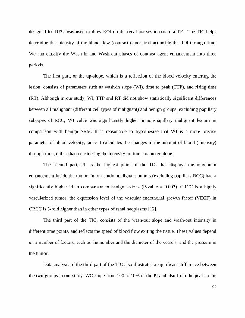
95
designed for IU22 was used to draw ROI on the renal masses to obtain a TIC. The TIC helps
determine the intensity of the blood flow (contrast concentration) inside the ROI through time.
We can classify the Wash-In and Wash-out phases of contrast agent enhancement into three
periods.
The first part, or the up-slope, which is a reflection of the blood velocity entering the
lesion, consists of parameters such as wash-in slope (WI), time to peak (TTP), and rising time
(RT). Although in our study, WI, TTP and RT did not show statistically significant differences
between all malignant (different cell types of malignant) and benign groups, excluding papillary
subtypes of RCC, WI value was significantly higher in non-papillary malignant lesions in
comparison with benign SRM. It is reasonable to hypothesize that WI is a more precise
parameter of blood velocity, since it calculates the changes in the amount of blood (intensity)
through time, rather than considering the intensity or time parameter alone.
The second part, PI, is the highest point of the TIC that displays the maximum
enhancement inside the tumor. In our study, malignant tumors (excluding papillary RCC) had a
significantly higher PI in comparison to benign lesions (P-value = 0.002). CRCC is a highly
vascularized tumor, the expression level of the vascular endothelial growth factor (VEGF) in
CRCC is 5-fold higher than in other types of renal neoplasms [12].
The third part of the TIC, consists of the wash-out slope and wash-out intensity in
different time points, and reflects the speed of blood flow exiting the tissue. These values depend
on a number of factors, such as the number and the diameter of the vessels, and the pressure in
the tumor.
Data analysis of the third part of the TIC also illustrated a significant difference between
the two groups in our study. WO slope from 100 to 10% of the PI and also from the peak to the
96
half of the WO slope had significantly higher values in non papillary RCC comparing to benign
SRM (P-values: 0.003 and 0.008 respectively). WO intensity at 30 seconds after the peak
showed a statistically significant difference between the two groups.
The neovascularization and shunts formed in malignant tumors explain the higher amount
of blood flow and contrast intensity inside RCC [90, 93]. All WI, PI, and WO parameters are
representatives of presumably increased blood flow and shunts in the tissue, and they confirm the
presence of large numbers of microvessels inside the malignant tumors due to neovascularization
[94]. Shigeyuki Aoki et al reported the only comparable study to ours in 2010. In that study, 30
renal cystic and solid tumors underwent CEUS using Sonazoid. Since some lesions were cystic,
or had small solid components, they placed multiple small ROI (3 mm each) and averaged their
values. Time To Peak (TTP) was significantly shorter among malignant lesions, while Wash In
(WI) slope was significantly higher in malignant lesions in that study [95]. Their results were
very similar to ours. However, in our study, parameter TTP was not statistically different
between the two groups, the other parameter of WI slope and Peak Intensity showed a higher
value in RCC group in comparison with benign group. Fig 25 and 26 summarize the steps and
parameters to differentiate malignant from benign SRM.
97
3. Logistic Regression Model
In the logistic regression part of the data analysis, combination of all variables was used
to find a logistic regression model that could predict the nature of the tumor by any combination
of qualitative and/or quantitative independent predictors.
Among all wash-in variables mentioned in the result chapter (PI, WI slope 5-45%, 10-
90%, and 50-100%), only PI could differentiate non-papillary RCC vs. benign SRM with Odds
ratio (OR) of 4.45.
Testing wash-out variables (WO slope 100-50%, 100-10%, and WO intensity at
peak+30s), WI slope 100-10% was the only variable to differentiate non-papillary RCC from
benign lesions with OR of 5.
Analyzing the combination of all wash-in and wash-out variables resulted in the same
outcome as analyzing the wash-out variables (wash-out 100-10% with the OR of 5).
Looking for a logistic regression model among qualitative variables, none of unenhanced
variables and only wash-out among enhancing variables could predict malignancy with OR of
4.5. All other combinations were unsuccessful in a search for a logistic regression model for
predicting malignancy, as explained in result chapter. However, logistic regression model can
not predict an independent variable in this group considering variables increased echogenicity
and hypovascularity had a value of zero amongst benign lesions.
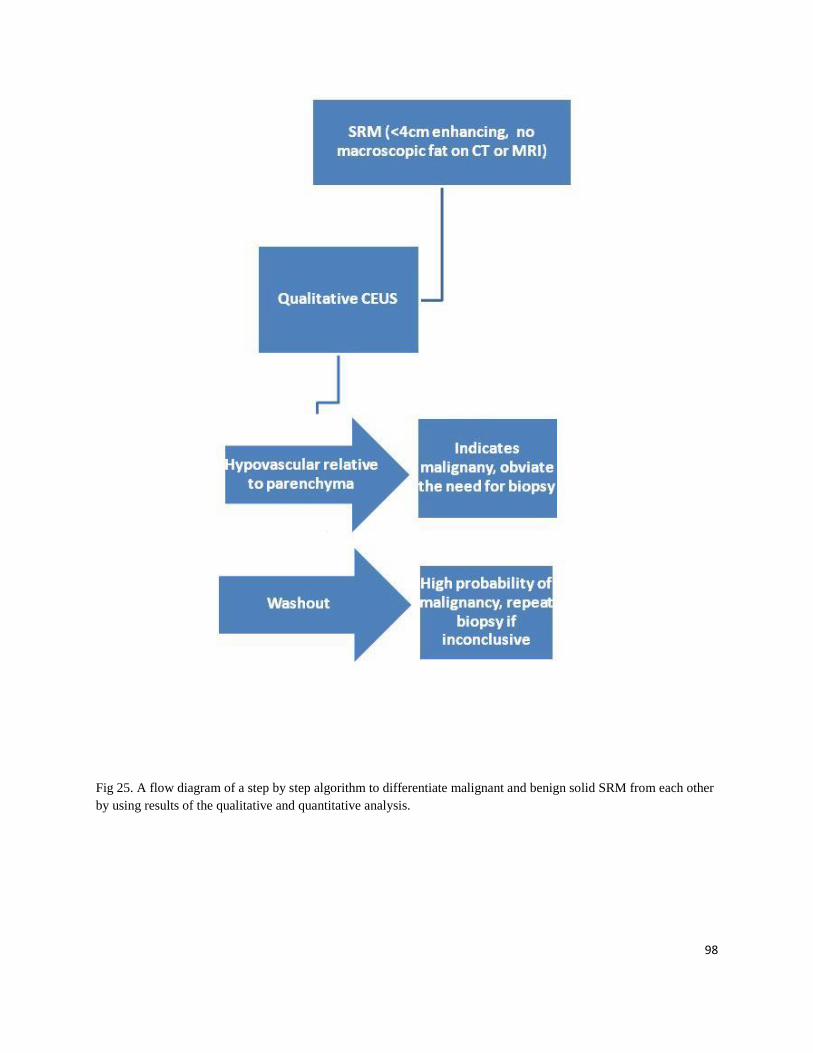
98
Fig 25. A flow diagram of a step by step algorithm to differentiate malignant and benign solid SRM from each other
by using results of the qualitative and quantitative analysis.

99
Chapter 6
Conclusion
The incidence of RCC in Canada and the United states is increasing, mostly in the SRM
category. Between 20 to 45% of small renal masses that are removed as RCC based on imaging,
turn out to be benign lesions on post-surgical pathology.
Most patients with newly detected renal tumors are evaluated with CT and less with MRI.
Both CT and MRI have limitations due to radiation exposure (CT), availability (MRI),
occurrence of allergic reactions to injected contrast medium, and concerns regarding the use of
contrast medium in patients with impaired renal function. With the exception of lipid-rich AML,
CT or MRI have difficulty differentiating lipid-poor AML and Oncocytoma from RCC. Tumor
biopsy can result in complication and has a lower yield in the population of SRM because of
their small size. Tissue sampling (biopsy) as a gold standard diagnostic tool has challenges when
it comes to the kidney. Because of the small size of the renal tumor, biopsy can be difficult and
there is the risk of complications, such as bleeding, and arterio-venous fistula. Concerns
regarding potential seeding of tumor persist.
CEUS is a promising, safe, and non invasive tool to evaluate the vascularity of SRM,
specifically in patients with renal insufficiency [77]. It can eliminate the need for further imaging
in complicated cysts by confirming the absence of flow. Moreover, in hypovascular solid lesions
that cannot be identified as solid on CT or MRI, CEUS can confirm the solid nature of these
lesions and therefore the need for further assessment. Our results show that a subgroup of
malignant SRM lesions can be accurately differentiated from benign lesions, which would
potentially obviate the need for biopsy.
100
Chapter 7
Future Directions
Contrast enhanced US technology is at its infancy with potential for expansion with
improved technology. Contrast agents more appropriate for different probe MHz are to be
developed and probe technology for contrast agent detections would evolve. There are currently
limitations to the motion compensation software as well as quantification tools. 3D acquisition
will improve more complete assessment of a lesion. We have attempted to determine imaging
features to differentiate benign from malignant renal lesions based on the known vascular
differences between these two groups of lesions.
1. Strengths
Most previous studies included small patient numbers, and focused on qualitative values,
and very few have acquired and analyzed quantitative parameters like TIC values. This study not
only has evaluated a comprehensive number of qualitative tumor parameters, it has also
compared all possible quantitative values derived from the TIC between benign and malignant
lesions.
2. Limitations:
One of the limitations of this study, and in general of the CEUS test, is that the quality of
imaging can be affected by the depth and location of the lesion. A poor ultrasonic window,
because of obesity, ribs, and the presence of bowel gas or location of the lesion interfere with
101
ultrasound scanning. Since the test involves an operative-dependant imaging modality, it requires
sufficient experience, skills, and training.
Quantitative assessment of these renal masses is challenging if an optimal imaging plane
that captures in-plane motion cannot be achieved, if both the lesion and renal parenchyma are not
on the same plane or if the patient can not cooperate. Robust motion compensation soft-ware
would be useful in these situations.
3. Future Work
Future work could include two directions: a) Improvement of the technique, and b) addition of
other concepts.
Based on our experience in this study, the following have been noted as imperative to further
exploration of Contrast-Enhanced Ultrasound:
a. Improvement in motion compensation tools: The motion correction tools that are
embedded in quantitative software programs are assigned to remove the effect of
breathing and any other movement from TIC of the lesion. The current motion
compensation tools do not capture the full difference between the TIC of benign and
malignant lesions. We believe more work could be the monitor done on quantitative
software designed to calculate the TICs.
2. Ability to acquire DICOM data from the monitor and evaluate data from different
machines with the same software: Currently, different ultrasound units acquire data in
different formats. Therefore, to be able to place ROI and draw TIC on each clip, one
should have access to the source data and the software specifically designed for that
ultrasound machine. Considering different software use different formulas to fit and
102
calculate TICs, reproducibility of quantitative results may be challenging. There is a need
to design a software that can acquire DICOM data from the monitor, and analyze the data
from the different machines.
3. Development of different modeling algorithms to fit TIC data: As mentioned above,
today‟s software use different algorithms to fit TIC, and therefore the results are affected
by the formula used in different software. Not all fitting options available on QLAB
worked to fit a TIC, and not all TICs were fitted well by A single fitting method. Shape
of a TIC and parameters in a formula affect the suitability of a fitting formula for a TIC.
Developing a fitting method that can fit a curve regardless of its shape improves the
consistency of TIC calculation.
4. Comparison of data from multiple machines on the same lesion: To make sure that the
results we obtained from this study are independent from the ultrasound unit we used, the
study should be repeated by comparing the acquired data from different units, and test the
inter-machine agreement.
With the collected data we aim to compare the quantitative values obtained using IU22,
Sequoia 512, and Aplio XG ultrasound machines to demonstrate that our results are
machine independent.
5. The aim of this study was to find a distinctive pattern in renal tumor microvasculature.
However, the presence of large feeding vessels and tissue necrosis in the imaging plane
made it difficult to locate the ROI and TIC free of the effect of macrovessels and

103
avascular areas. Development of software that can detect and remove necrosis and large
vessels from the ROI will increase the accuracy of the TIC assessment.
6. Assessment of the entire volume of tumor vasculature to avoid the influence of
heterogeneity, especially in the longitudinal assessment of tumors. Although current
sampling of a lesion is better representative a volume of a lesion than a small biopsy
sample, 3D acquisition will allow more complete assessment of the lesion potentially
improving reproducibility of the results.
7. Evaluating inter-observer agreement of qualitative analysis: The qualitative part of this
study (visual assessment of hemodynamics of the tumors) is subjective. Review of the
data by a panel of radiologists, especially with respect to the features with high
probability of malignancy such as the degree of vascularity relative the renal parenchyma
and presence of wash-out, would confirm reproducibility of our results. Moreover, more
objective assessment of vascularity and wash-out should be evaluated by the analysis of
the TIC data.
8. Correlation of CEUS findings with pathology: With the advent of 3D acquisition,
correlation can be performed between CEUS findings and pathology on the removed
lesions.
9. Comparison of longitudinal changes in the flow parameters with final histology: In
lesions that undergo observation, the baseline features and change in the hemodynamic
104
parameters of these lesions on CEUS on a longitudinal study can potentially identify
lesions with more aggressive behavior.
105
References
1. Xu, Z.F., et al., Renal cell carcinoma: real-time contrast-enhanced ultrasound findings. Abdom
Imaging, 2010. 35(6): p. 750-6.
2. Khamanarong, K., et al., Anatomy of renal arterial supply. Clin Anat, 2004. 17(4): p. 334-6.
3. Hallgrmsson, b., The kidney: From normal development to congenital disease, in The kidney:
From normal development to congenital disease. J.V. Bard, Peter D.; Woolf, Adrian S., Editor.
2003, Academic Press: Boston.
4. Birnbaum, B.A., et al., Renal cyst pseudoenhancement: influence of multidetector CT
reconstruction algorithm and scanner type in phantom model. Radiology, 2007. 244(3): p. 767-
75.
5. Pantuck, A.J., A. Zisman, and A.S. Belldegrun, Urologic oncology: extraordinary opportunities
for discovery: highlights from the 2nd annual winter meeting of the society of urologic oncology
december 1-2, 2001, bethesda, MD. Rev Urol, 2003. 5(1): p. 26-8.
6. Nguyen, M.M., I.S. Gill, and L.M. Ellison, The evolving presentation of renal carcinoma in the
United States: trends from the Surveillance, Epidemiology, and End Results program. J Urol,
2006. 176(6 Pt 1): p. 2397-400; discussion 2400.
7. Lee, C.T., et al., Surgical management of renal tumors 4 cm. or less in a contemporary cohort. J
Urol, 2000. 163(3): p. 730-6.
8. Israel, G.M. and M.A. Bosniak, How I do it: evaluating renal masses. Radiology, 2005. 236(2): p.
441-50.
9. Silverman, S.G., et al., Management of the incidental renal mass. Radiology, 2008. 249(1): p. 16-
31.
10. Frank, I., et al., Solid renal tumors: an analysis of pathological features related to tumor size. J
Urol, 2003. 170(6 Pt 1): p. 2217-20.
11. Chawla, S.N., et al., The natural history of observed enhancing renal masses: meta-analysis and
review of the world literature. J Urol, 2006. 175(2): p. 425-31.
12. Siu, W., et al., Growth rates of renal cell carcinoma and oncocytoma under surveillance are
similar. Urologic Oncology, 2007. 25(2): p. 115-9.
13. Kunkle, D.A., et al., Enhancing renal masses with zero net growth during active surveillance. J
Urol, 2007. 177(3): p. 849-53; discussion 853-4.
14. Rubio Briones, J. and F. Algaba, Management of small renal masses. Adv Urol, 2008: p. 606401.
106
15. Chow, W.H. and S.S. Devesa, Contemporary epidemiology of renal cell cancer. Cancer J, 2008.
14(5): p. 288-301.
16. Lane, B.R., What is the best method of preoperatively determining the management of small renal
masses? J Urol, 2011. 186(1): p. 12-3.
17. Stakhovskyi, O., et al., Small renal mass: what the urologist needs to know for treatment planning
and assessment of treatment results. AJR. American Journal of Roentgenology, 2011. 196(6): p.
1267-73.
18. Gill, I.S., et al., Clinical practice. Small renal mass. N Engl J Med, 2010. 362(7): p. 624-34.
19. Carrizosa DR, G.P., Epidemiology and screening of renal cell carcinoma. 2009.
20. Reeves, G.K., et al., Cancer incidence and mortality in relation to body mass index in the Million
Women Study: cohort study. BMJ, 2007. 335(7630): p. 1134.
21. Lipworth, L., R.E. Tarone, and J.K. McLaughlin, The epidemiology of renal cell carcinoma.
Journal of Urology, 2006. 176(6 Pt 1): p. 2353-8.
22. Cho, E., et al., Prospective evaluation of analgesic use and risk of renal cell cancer. Archives of
Internal Medicine, 2011. 171(16): p. 1487-93.
23. Gago-Dominguez, M., et al., Regular use of analgesics is a risk factor for renal cell carcinoma.
British Journal of Cancer, 1999. 81(3): p. 542-8.
24. Kojima, Y., et al., Renal cell carcinoma in dialysis patients: a single center experience. Int J Urol,
2006. 13(8): p. 1045-8.
25. Kliem, V., et al., Risk of renal cell carcinoma after kidney transplantation. Clin Transplant, 1997.
11(4): p. 255-8.
26. Ianhez, L.E., et al., Renal cell carcinoma in renal transplant patients. Urology, 2007. 69(3): p.
462-4.
27. Yuan, J.M., et al., Hypertension, obesity and their medications in relation to renal cell carcinoma.
British Journal of Cancer, 1998. 77(9): p. 1508-13.
28. Wein, CAmpbell-Walsh Urology. 2011.
29. Polascik, T.J., D.G. Bostwick, and P. Cairns, Molecular genetics and histopathologic features of
adult distal nephron tumors. Urology, 2002. 60(6): p. 941-6.
30. Cheng, W.S., G.M. Farrow, and H. Zincke, The incidence of multicentricity in renal cell
carcinoma. J Urol, 1991. 146(5): p. 1221-3.
31. Delahunt, B., et al., Morphologic typing of papillary renal cell carcinoma: comparison of growth
kinetics and patient survival in 66 cases. Hum Pathol, 2001. 32(6): p. 590-5.
32. Novick AC, B.R., Campbell SC, Renal tumours. Campbell-Walsh Urology. ed. K.L. Wein AJ,
Novick AC, Partin and P.C. AV. 2007, Philadelphia.
107
33. B. Ljungberg, N.C., D.C. Hanbury, M. Hora, M.A. Kuczyk, and P.F.A.M. A.S. Merseburger, J-J.
Patard, I.C. Sinescu, Guidelines on Renal Cell Carcinoma. 2010.
34. Lee, C.T., et al., Mode of presentation of renal cell carcinoma provides prognostic information.
Urol Oncol, 2002. 7(4): p. 135-40.
35. Kutikov, A., et al., Incidence of benign pathologic findings at partial nephrectomy for solitary
renal mass presumed to be renal cell carcinoma on preoperative imaging. Urology, 2006. 68(4): p.
737-40.
36. Pettus, J.A., et al., Effect of baseline glomerular filtration rate on survival in patients undergoing
partial or radical nephrectomy for renal cortical tumors. Mayo Clin Proc, 2008. 83(10): p. 1101-6.
37. Kovacs, G., et al., The Heidelberg classification of renal cell tumours. J Pathol, 1997. 183(2): p.
131-3.
38. National Institute of Cancer (NIC). 2012.
39. Lang, K., et al., The burden of illness associated with renal cell carcinoma in the United States.
Urol Oncol, 2007. 25(5): p. 368-75.
40. Shields, M., M.D. Carroll, and C.L. Ogden, Adult obesity prevalence in Canada and the United
States. NCHS Data Brief, 2011(56): p. 1-8.
41. P.H.A.o., Obesity In Canada. 2009.
42. Clague, J., et al., Family history and risk of renal cell carcinoma: results from a case-control study
and systematic meta-analysis. Cancer Epidemiol Biomarkers Prev, 2009. 18(3): p. 801-7.
43. Gudbjartsson, T., et al., A population-based familial aggregation analysis indicates genetic
contribution in a majority of renal cell carcinomas. Int J Cancer, 2002. 100(4): p. 476-9.
44. A. Abugaber, K.L., N. Danchenko, D. Thompson, T. Bhardwaj, G. Bjarnason, A. Finelli, A.
Kapoor, B. Jaszewski, Cost of illness of renal cell carcinoma in Canada. Journal of Clinical
Oncology, 2007. 25(18S).
45. Postema, M. and O.H. Gilja, Contrast-enhanced and targeted ultrasound. World J Gastroenterol,
2011. 17(1): p. 28-41.
46. Postema, M. and G. Schmitz, Bubble dynamics involved in ultrasonic imaging. Expert Rev Mol
Diagn, 2006. 6(3): p. 493-502.
47. Webb, A., Introduction to biomedical imaging. 2003: Hoboken, NJ : Wiley [u.a.], 2003.
48. Postema, M. and O.H. Gilja, Ultrasound-directed drug delivery. Curr Pharm Biotechnol, 2007.
8(6): p. 355-61.
49. Voigt, J.U., Ultrasound molecular imaging. Methods, 2009. 48(2): p. 92-7.
50. ter Haar, G., Safety and bio-effects of ultrasound contrast agents. Med Biol Eng Comput, 2009.
47(8): p. 893-900.
108
51. Schmitz, G., Improvement of ultrasound compound imaging by speed-of-sound estimation.
Biomed Tech (Berl), 2002. 47 Suppl 1 Pt 1: p. 430-3.
52. Averkiou, M., et al., Ultrasound contrast imaging research. Ultrasound Q, 2003. 19(1): p. 27-37.
53. Qin, S., C.F. Caskey, and K.W. Ferrara, Ultrasound contrast microbubbles in imaging and
therapy: physical principles and engineering. Phys Med Biol, 2009. 54(6): p. R27-57.
54. Jayaweera, A.R., et al., In vivo myocardial kinetics of air-filled albumin microbubbles during
myocardial contrast echocardiography. Comparison with radiolabeled red blood cells. Circ Res,
1994. 74(6): p. 1157-65.
55. Postema, M., A. Bouakaz, and N. de Jong, Noninvasive microbubble-based pressure
measurements: a simulation study. Ultrasonics, 2004. 42(1-9): p. 759-62.
56. Schutt, E.G., et al., Injectable microbubbles as contrast agents for diagnostic ultrasound imaging:
the key role of perfluorochemicals. Angew Chem Int Ed Engl, 2003. 42(28): p. 3218-35.
57. Dayton, P.A. and J.J. Rychak, Molecular ultrasound imaging using microbubble contrast agents.
Front Biosci, 2007. 12: p. 5124-42.
58. Correas, J.M., et al., The kidney: imaging with microbubble contrast agents. Ultrasound Q, 2006.
22(1): p. 53-66.
59. Ziegler, L. and R.T. O'Brien, Harmonic ultrasound: a review. Vet Radiol Ultrasound, 2002. 43(6):
p. 501-9.
60. Lindner, J.R., Microbubbles in medical imaging: current applications and future directions. Nat
Rev Drug Discov, 2004. 3(6): p. 527-32.
61. Goldberg, B.B., J.B. Liu, and F. Forsberg, Ultrasound contrast agents: a review. Ultrasound in
Medicine & Biology, 1994. 20(4): p. 319-33.
62. Choyke, P.L., M.V. Knopp, and S.K. Libutti, Special techniques for imaging blood flow to
tumors. Cancer J, 2002. 8(2): p. 109-18.
63. Jain, R.K., Understanding barriers to drug delivery: high resolution in vivo imaging is key. Clin
Cancer Res, 1999. 5(7): p. 1605-6.
64. Folkman, J., Tumor angiogenesis. Adv Cancer Res, 1974. 19(0): p. 331-58.
65. Folkman, J., Tumor angiogenesis: therapeutic implications. N Engl J Med, 1971. 285(21): p.
1182-6.
66. Jain, R.K., Delivery of molecular and cellular medicine to solid tumors. J Control Release, 1998.
53(1-3): p. 49-67.
67. Haers, H., et al., Contrast harmonic ultrasonographic appearance of focal space-occupying renal
lesions. Vet Radiol Ultrasound, 2010. 51(5): p. 516-22.
109
68. Rendon, R.A. and M.A. Jewett, Expectant management for the treatment of small renal masses.
Urol Oncol, 2006. 24(1): p. 62-7.
69. Xu, Z.F., et al., Renal cell carcinoma and renal angiomyolipoma: differential diagnosis with real-
time contrast-enhanced ultrasonography. J Ultrasound Med, 2010. 29(5): p. 709-17.
70. Jiang, J., et al., Clear cell renal cell carcinoma: contrast-enhanced ultrasound features relation to
tumor size. Eur J Radiol, 2010. 73(1): p. 162-7.
71. Williams, R., et al., Dynamic microbubble contrast-enhanced US to measure tumor response to
targeted therapy: a proposed clinical protocol with results from renal cell carcinoma patients
receiving antiangiogenic therapy. Radiology, 2011. 260(2): p. 581-90.
72. Lassau, N., et al., Advanced hepatocellular carcinoma: early evaluation of response to
bevacizumab therapy at dynamic contrast-enhanced US with quantification--preliminary results.
Radiology, 2011. 258(1): p. 291-300.
73. Bogaard, J.M., et al., Random walk type models for indicator-dilution studies: comparison of a
local density random walk and a first passage times distribution. Cardiovasc Res, 1986. 20(11): p.
789-96.
74. Lassau, N., et al., Dynamic contrast-enhanced ultrasonography (DCE-US): a new tool for the
early evaluation of antiangiogenic treatment. Target Oncol, 2010. 5(1): p. 53-8.
75. Tamai, H., et al., Contrast-enhanced ultrasonography in the diagnosis of solid renal tumors. J
Ultrasound Med, 2005. 24(12): p. 1635-40.
76. Saunders, J.H., Dorland's Medical Dictionary for Health Consumers, in Dorland's Medical
Dictionary for Health Consumers 2007, Elsevier Inc.
77. Ascenti, G., et al., Contrast-enhanced second-harmonic sonography in the detection of
pseudocapsule in renal cell carcinoma. AJR Am J Roentgenol, 2004. 182(6): p. 1525-30.
78. EbleJN, S.G., Epstein JI, Sesterhenn IA, Pathology and Genetics of Tumours of the Urinary
System and Male Genital Organs. Vol. 7. 2004, Lyon: IARC. 359.
79. Prasad, S.R., et al., Common and uncommon histologic subtypes of renal cell carcinoma: imaging
spectrum with pathologic correlation. Radiographics, 2006. 26(6): p. 1795-806; discussion 1806-
10.
80. Bosniak, M.A., The current radiological approach to renal cysts. Radiology, 1986. 158(1): p. 1-
10.
81. Siegel, C.L., A.J. Fisher, and H.F. Bennett, Interobserver variability in determining enhancement
of renal masses on helical CT. AJR Am J Roentgenol, 1999. 172(5): p. 1207-12.
82. Lee, K.H., et al., Triple-phase MDCT of hepatocellular carcinoma. AJR Am J Roentgenol, 2004.
182(3): p. 643-9.
110
83. Wong, K., et al., Angiomyolipoma of the kidney: a clinical enigma in diagnosis and management.
Ann R Coll Surg Engl, 1992. 74(2): p. 144-8.
84. Ignee, A., et al., Contrast enhanced ultrasound of renal masses. World J Radiol, 2010. 2(1): p. 15-
31.
85. Brian S. Garra, M.D., Renal Study Using Speckle Reduction Imaging. 2004.
86. Haendl, T., et al., [Renal cell cancer does not show a typical perfusion pattern in contrast-
enhanced ultrasound]. Ultraschall Med, 2009. 30(1): p. 58-63.
87. Baish, J.W. and R.K. Jain, Fractals and cancer. Cancer Res, 2000. 60(14): p. 3683-8.
88. Huang, B.-J.L., Cong | Fan, Pei-Li | Han, Hong | Yuan, Hai-Xia | Jin, Yun-Jie | Wang, Wen-Ping,
The value of contrast-enhanced ultrasonography in subtypes differentiation of renal cell
carcinoma. Chinese Journal of Medical Ultrasound, 2011. 8(5): p. 4.
89. Reese, J.H., Renal cell carcinoma. Curr Opin Oncol, 1992. 4(3): p. 427-34.
90. Lam, J.S., et al., Clinicopathologic and molecular correlations of necrosis in the primary tumor of
patients with renal cell carcinoma. Cancer, 2005. 103(12): p. 2517-25.
91. Yamashita, Y., et al., Detection of pseudocapsule of renal cell carcinoma with MR imaging and
CT. AJR Am J Roentgenol, 1996. 166(5): p. 1151-5.
92. Newhouse, J.H. and B.J. Wagner, Renal oncocytomas. Abdom Imaging, 1998. 23(3): p. 249-55.
93. Qian, C.N., et al., Complexity of tumor vasculature in clear cell renal cell carcinoma. Cancer,
2009. 115(10 Suppl): p. 2282-9.
94. Furuya, M. and Y. Yonemitsu, Cancer neovascularization and proinflammatory
microenvironments. Curr Cancer Drug Targets, 2008. 8(4): p. 253-65.
95. Aoki, S., et al., Contrast-enhanced ultrasound using a time-intensity curve for the diagnosis of
renal cell carcinoma. BJU Int, 2011. 108(3): p. 349-54.
96. Thompson RH, Kurta JM, Kaag M, Tickoo SK, Kundu S, Katz D, Nogueira L, Reuter VE, Russo
P., Tumor size is associated with malignant potential in renal cell carcinoma cases Urol. 2009
May;181(5):2033-6.