the value of flexibility in offshore oil field development
TRANSCRIPT

NTNU Trondheim Norges teknisk-naturvitenskapelige
universitet
Doktor ingenieravhandling 1997:69 Institutt for industriell okonomi og
teknologiledelse
1037

THE VALUE OF FLEXIBILITY IN OFFSHORE
OIL FIELD DEVELOPMENT PROJECTS
Morten W. Lund
Department of Economics and Technology Management
The Norwegian University of Science and Technology
Trondheim
June 1997


DISCLAIMER
Portions of this document may be illegible in electronic image products. Images are produced from the best available original document.

Abstract
ABSTRACT
The main objective of this thesis has been to identify the value of flexibility in offshore oil field development projects. Uncertainty surrounding the development is often substantial, and the operator’s possibility to take corrective actions during the project is correspondingly of significant value. Flexibility should thus be given due attention when the development and depletion strategy is selected.
Estimates obtained from exploration wells can be dependent through common information. The effect of stochastic dependence was illustrated by an analytical model, where the dependence was expressed in terms of correlation between estimate errors. The results showed that a high degree of correlation might distort the benefit of additional exploration.
A prototype that covered the major phases of the project was developed to study the value of flexibility. The prototype was a Markov decision process, solved by stochastic dynamic programming. Based on discussions with Norwegian oil companies, three uncertain variables were addressed; the reservoir volume, the well rate, and the oil price. In order to obtain a compact model, simple descriptions were used to mimic the uncertainty. The reservoir was thus depicted as a tank model, and the well rate and the oil price were assumed to follow Markov processes. Flexibility was restricted to managerial, as opposed to financial, flexibility.
Application of the prototype to a case study, based on an ongoing field development, showed that flexibility might be of considerable value to the project. Particularly capacity flexibility and initiation flexibility were identified as important aspects of the development. The results also emphasised the importance of a joint assessment, as the values of different flexibility types are not additive.
In conclusion, the proposed model provides motivation for further development of the decision support systems presently available. Future decision making should therefore be made within a framework which gives consideration to flexibility.
i


Preface
PREFACE
The work reported in this thesis has been done at the Department of Economics and Technology Management at the Norwegian University of Science and Technology. The work as been supported by a grant from the research programme Project 2000.
I wish to express my gratitude to my professional supervisor, Professor Einar Matson, for his support and encouragement.
Furthermore I want to thank former and present colleagues at SINTEF Industrial Management - Applied Economics, for all help during the work. Especially I would like to thank Mr. Kjetil K. Haugen and Mr. Thor H. Bjprkvoll. Both have taken great interest in my work, and have contributed significantly to the completion of this thesis through constructive criticism.
Finally I would like to offer thanks to colleagues at North Carolina State University, who shared their knowledge with me. I appreciate all their help.
Trondheim, June 1997
Morten W. Lund
m


Contents
CONTENTS
Abstract................................................................... iPreface............................................................................................................................. iiiContents.............................................................................................................................v
1 INTRODUCTION.... ...........................................................................................11.1 Historical background.......................................................................................... 11.2 The future..............................................................................................................51.3 Focus on flexibility............................................................................................... 81.4 Outline................................................................................................................ 10
2 THE RESEARCH DOMAIN........................................................................... 132.1 The research problem......................................................................................... 13
2.1.1 Background............................................................................................ 132.1.2 Problem...................................................................................................17
2.2 Contribution of this research............................................................................. 192.3 Assumptions and limitations............................................................................. 202.4 Conversion factors.............................................................................................22
3 FLEXIBILITY................................................................................................... 233.1 Definition of flexibility.......................................................................................233.2 The value of flexibility......................................................................................24
3.2.1 Comparing flexibility............................................................................243.2.2 Definition of value of flexibility.......................................................... 263.2.3 An example of the value of flexibility.................................................27
3.3 Types of flexibility........................................................................................... 313.3.1 Initiation flexibility............................................................................... 333.3.2 Termination flexibility..........................................................................363.3.3 Start/stop flexibility.............................................................................. 383.3.4 Capacity flexibility................................................................................ 40
3.4 Evaluation of flexibility.................................................................................... 433.4.1 Analyses of flexibility and its value.....................................................433.4.2 Combining flexibility types................................................................. 44
3.5 Concluding remarks...........................................................................................46
v

Contents
4 MODELLING THE OFFSHORE OIL FIELDDEVELOPMENT PROJECT.... .......................................................................47
4.1 Introduction........................................................................................................ 474.2 Going from a deterministic to a stochastic model...........................................494.3 Some modelling considerations.........................................................................50
4.3.1 Simplifying the problem description................................................... 514.3.2 Requirements to the solution method.................................................. 54
4.4 Alternative methods.......................................................................................... 554.4.1 Foundation and terminology................................................................. 554.4.2 Contingent claims analysis....................... 564.4.3 Stochastic dynamic programming........................................................584.4.4 Scenario aggregation.............................................................................60
4.5 Why use stochastic dynamic programming?................................................... 614.5.1 Discarding CCA........................................ 614.5.2 Solving the field development project by scenario aggregation....... 624.5.3 The choice of SDP.................................................................................644.5.4 Criticism of SDP....................................................................................68
4.6 A simplified field development description.................................................... 694.6.1 Phases.....................................................................................................704.6.2 Stochastic variables...............................................................................724.6.3 Flexibility................................................................................................77
4.7 Summing up....................................................................................................... 80
5 THE RESERVOIR.............................................................................................835.1 Introduction......................................................................................................... 835.2 Reservoir models................ 855.3 Models of the reservoir under certainty............................................................86
5.3.1 Tank models.............................................. 865.3.2 Two-dimensional models.......................... 88
5.4 Models of the reservoir under uncertainty....................................................... 905.4.1 Production profiles based on reservoir models.................................. 915.4.2 Modelling the production profile..........................................................92
5.5 A simple reservoir model............................................................ 935.6 Uncertainty resolution....................................................................................... 985.7 Exploration........................................................................................................ 100
5.7.1 Introduction........................................................................................ 101
vi

Contents
5.7.2 Dependent information....................................................................... 1025.8 An exploration model with dependent information...................................... 103
5.8.1 The problem, assumptions and notation............................................1035.8.2 Variance of the posterior distribution................................................ 1065.8.3 Determining optimal exploration effort.............................................Ill
5.9 A numerical example.......................................................................................1125.10 Correlation caused by overlapping information.............................................1175.11 Comments on the exploration model..............................................................1215.12 Summing up......................................................................................................123
6 OIL PRICE FORECASTING AND MODELLING..................................... 1256.1 Introduction.......................................................................................................1256.2 A historic review.............................................................................................. 1256.3 Alternative views............................................................................................. 1286.4 Scenario/qualitative models............................................................................ 1296.5 Economic models............................................................................................. 1306.6 Stochastic processes......................................................................................... 132
6.6.1 Brownian motion.................................................................................1336.6.2 Mean reverting process....................................................................... 1356.6.3 Empirical and theoretical guidance.................................................... 137
6.7 Forecasting in retrospect..................................................................................1406.8 An applicable approach...................................................................................1436.9 Approximation of continuous stochastic processes.......................................146
6.9.1 Formulation.......................................................................................... 1466.9.2 Demands on the approximation......................................................... 146
6.10 Approximation of the geometric Brownian motion.......................................1476.11 Approximation of the Omstein-Uhlenbeck process................... 149
6.11.1 Approximation by an Ehrenfest urn model........................................1496.11.2 Multi-step transition probabilities...................................................... 1536.11.3 Performance of the approximation..................................................... 155
6.12 Concluding remarks................................................................. 156
7 A UNIFIED MODEL FOR VALUING FLEXIBILITY............................... 1577.1 Introduction.......................................................................................................1577.2 The stages.........................................................................................................1587.3 Decisions........................................................................................................... 159
7.3.1 The exploration phase......................................................................... 159
vii

Contents
7.3.2 The conceptual study phase.................................................................1607.3.3 The engineering and construction phase............................................ 1607.3.4 The production phase........................................................................... 1617.3.5 Phase independent decisions.............................................................. 162
7.4 State variables................................................................................................... 1627.4.1 Probability distribution of the reservoir volume................................1627.4.2 Platform capacity................................................................................. 1657.4.3 Production wells.................................................................................. 1667.4.4 Accrued reservoir information............................................................ 1667.4.5 Well rate............................................................................................... 1677.4.6 Oil price................................................................................................ 167
7.5 Mathematical representation...........................................................................1687.5.1 Subscripts............................................................................................. 1687.5.2 Decision variables................................................................................ 1697.5.3 Constants.................................................... 1707.5.4 Deduced variables....................................... 1727.5.5 The fundamental equation of optimality............................................ 1727.5.6 The immediate return function........................................................... 1737.5.7 Constraints............................................................................................173
7.6 Program structure.............................................................................................1767.7 Model performance........................................................................................ 179
7.7.1 Size of implemented model................................................................ 1797.7.2 Solution time and intermediate data storage...................................... 181
7.8 Summing up......................................................................................................184
8 APPLICATION OF THE MODEL TO AN OILFIELD DEVELOPMENT PROJECT............................................................ 185
8.1 Introduction....................................................................................................... 1858.2 The oil field development project................................................................... 186
8.2.1 General description.............................................................................. 1868.2.2 Decision epoch............................................ 1888.2.3 Annual rate of return................................... 1888.2.4 Oil price....................................................... 1898.2.5 Reservoir............................................................................................... 1908.2.6 Exploration...........................................................................................1918.2.7 Platform................................................................................................ 1928.2.8 Production.............................................................................................194
viii

Contents
8.2.9 Abandonment.......................................................................................1948.3 Value of flexibility - base case........................................................................ 1958.4 Value of different flexibility types..................................................................198
8.4.1 Sensitivity to reservoir volume uncertainty.......................................1998.4.2 Sensitivity to well rate uncertainty..................................................... 2018.4.3 Sensitivity to initial oil price..................................................... 204
8.5 Discussion.........................................................................................................2088.5.1 Flexibility types................................................................................... 2088.5.2 Stochastic variables............................................................................. 2108.5.3 Generalisation............................................................................;.......212
8.6 Concluding remarks.........................................................................................213
9 CONCLUSION AND DISCUSSION..............................................................2159.1 Introduction........................................................................................................2159.2 Results...............................................................................................................215
9.2.1 Model development............................................................................2159.2.2 Value of flexibility.............................................................................. 2169.2.3 Decision support................................................................................. 217
9.3 Future decision making................................................................................... 2179.4 Further research and model development...................................................... 219
9.4.1 Methodology.......................................................................................2199.4.2 Project environment............................................................................ 2209.4.3 Model extensions................................................................................ 220
9.5 Final remarks................................................................................................... 221
REFERENCES.................................................................................. .........................223
APPENDIX A NON-ADDITIVITY OF VALUE OF FLEXIBILITY..................235A. 1 A simple example.............................................................................................235A. 2 The value of added flexibility.......................................................................... 239
APPENDIX B UPPER LIMIT ON THE CORRELATION COEFFICIENT...... 241B. 1 Deriving the limit..............................................................................................241
APPENDIX C APPROXIMATION OF THE ORNSTEIN-UHLENBECKPROCESS BY A SCALED EHRENFEST URN MODEL...........243
C. 1 The Omstein-Uhlenbeck process.....................................................................243
IX

Contents
C. 2 Approximation by an Ehrenfest urn model................................................... 244
APPENDIX D APPROXIMATION ERROR..........................................................249D. 1 The error of the approximating process........................................................ 249
APPENDIX E ACTION SPACE.............................................................................253
x

1. Introduction
1 INTRODUCTION
1.1 Historical background
The start of the Norwegian offshore activity can be dated back to the early 1960’s when Phillips Petroleum Company launched an application to the Norwegian Ministry of Industry for wildcat drilling on the Norwegian continental shelf. The areas along the coast of Norway were brought into focus some years earlier by the discovery in 1958 of the large Groningen gas field in the Netherlands. Few, though, believed that economically viable resources, if any, existed on the Norwegian continental shelf at that time. The now rather famous letter from the Norwegian Geological Surveys to the Ministry of Foreign Affairs in Februaiy the same year is an illustrative example of the common view. It stated in unequivocal terms that “one could disregard the possibility of coal, oil, or sulphur deposits being present on the continental shelf along the Norwegian coast”.
In the years to follow the approach made by Phillips in 1962, the activity expanded. During the years 1963 and 1964 a total of 20 exploration licences were granted by the Norwegian Government, and in Autumn 1965 the first 22 production licences were awarded to nine companies or company groups. However, it still took another five years before the commercial break trough took place. In spring 1970, the discovery of the Ekofisk field was declared commercial, and in 1971 test production was started. Within a few years two additional large reserves were discovered. This was the Frigg gas reservoir in 1971, and the Statfjord field in 1974. Together with the Ekofisk field these two discoveries later turned out to be the major fields on the Norwegian continental shelf. The size and expected profitability of these fields strengthened the belief and stimulated investments in exploration for oil and gas on the Norwegian shelf (Hansen et al (1982)).
During the mid 70’s the concept of an annual production of 90 million tons oil equivalents (toe) was introduced as an illustration of a moderate production rate. The rate was mainly based on what was then seen to be the production level in the beginning of the 1980’s. In retrospect, it is evident that this objective was not a
1

1. Introduction
sustainable one. Since the production start-up of the Ekofisk field in 1971 the annual production of oil and NGL has increased steadily as shown in figure 1.1, to reach a level of approximately 165 million Sm3 oil equivalents (oe)1 in 1995. The production of gas has not experienced the same development, but has remained stable with minor fluctuations about 26 million Sm3 oe per year for the last decade. In the years to come this situation is expected to change. From a mere share of approximately 14% in 1995/1996, gas is expected to constitute about one third of the total petroleum production in year 2006 (NOE (1996)).
160 -
140 -
x 120 -
100 -
1 60 -
g 40 -
CM CO CD Ococococococococo CO O) O) O) O) O) 0)0 0)0)0)0) O) O)
Oil/NGLGas
Year
Fig. 1.1 Production of oil/NGL and gas. Source: NOE (1996).
The increase in total production has been accompanied by an increase in the number of companies involved in the oil production. From a few companies in the early years, the number of operators by the end of 1996 amounted to 17. In addition 9 other licensees were involved. However, equally important is the activity related to the offshore industry and its significance to the Norwegian economy. After the first drilling took place in the North Sea, several years elapsed before any noticeable effect reached the mainland in the form of increased employment and sub supplies. But, as the industry grew, the offshore activity was reflected also onshore, giving nourishment to a vast variety of industries and trade and services.
1 1 Sm3 oe = 0.84 toe.
2

1. Introduction
The time from discovery of a field to start of production may vary substantially, but typically covers several years. For fields on the Norwegian continental shelf the relevant time lags range from approximately 3 (Ekofisk) to 23 (Sleipner Vest) years, with an average of 9 years (Oljedirektoratet (1995)2). Compared to most industrial projects this is a long horizon. In addition to the time from discovery to production the project duration includes the subsequent production period, which, in itself, may last a few decades. For instance are all the three fields that first were developed (Ekofisk, Frigg and Statjord) still producing. The total project period, i.e., from discovery to abandonment of the field, can therefore be of substantial length.
In line with this the investment expenditures represent considerable amounts. The complete investments on the Norwegian continental shelf, including pipelines, have over the last years been around NOK 30 billion per year. Even though one recently has seen an increase to about NOK 50 - 60 billion (1993 - 1994) it is expected that the bulk of investments have been completed and that future investments will decrease. However, new discoveries are necessarily hard to predict and the assumption of a downward sloping trend in total investments is a fragile one. Figure1.2 shows total (expected) investments for Norwegian fields in production and to be developed. The fields under development represent investments in the range of NOK1.3 to 34.1 billion.
The statement “Norway must not become another Kuwait” has been put forward in many discussions regarding the strategy for the Norwegian offshore activity. Nevertheless, the dependence of the Norwegian economy on the revenue from the oil industry is indisputable. In the 1990's, exports of oil and gas have represented about one third of the total Norwegian exports, and the activity has provided between 14 and 15 percent of the gross national product (table 1.1). The figures clearly illustrate the major importance of the industry.
2 Oljedirektoratet - the Norwegian Petroleum Directorate.
3

1. Introduction
100 -r
90
80
70
60
50
40
30
20
10
0Fields in production Fields to be developed
Fig. 1.2 Total expected investments in NOK 1994 billion for fields on the Norwegian continental shelf. Fields divided between Norway and U.K.3 are represented by the Norwegian part of the investments. Source: NOE (1995).
Tab. 1.1 Principal figures for the oil and gas activity. [NOK million]1990 1991 1992 1993 1994
Exports of crude petroleum and natural gas (E_Cp&Ng) 88 540 96 704* 97 158* 104 069* 107 312*E_Cp&Ng / Total exports 0.30 . 0.31 0.32 0.33 0.32GDP - oil activity (GDP_Oa) 96 926 102 908 104 213 109 248 111 618*GDP_Oa/Total GDP 0.14 0.15 0.14 0.14 0.14*: Provisional or preliminary figure
Source: Statistics Norway (1995)
Norway has also become a major agent in the world oil and gas market, and was in 1995 the worlds 9th largest oil producer. Partly due to a relatively small domestic consumption Norway is positioned in the forefront among the net oil exporters, only beaten by Saudi Arabia. The 2.7 million barrels that on average are exported each day are mainly send to Western Europe, with great Britain, The Netherlands, 3
3 Murchison and Statfjord.
4

1. Introduction
Germany and France as the main buyers (57.2% in 1995). A fraction (5.6% in 1995) is exported to North America. A similar position is obtained also in the international gas market, where Norway is ranked among the ten largest exporters. All exported gas is transported to Western Europe, and Norway provides about nine percent of the consumption of Western Europe. In 1995 the total export volume amounted to 27.6 million Sm3 oe.
1.2 The future
The position of the Norwegian oil and gas industry, in particular in the domestic economy, and it’s profit potential, has lead to a close monitoring of the industry’s performance. The search for cost efficient solutions and optimal development strategies has strengthened over the last years as the fields have become economically marginal and more demanding to develop. As a consequence of the declining size the fields have turned less profitable.
In the early years of the Norwegian oil history the situation was different. The development of fields was characterised by high uncertainty, but, at the same time, was also considered to have enormous potential. Revenues from the fields were large, and development costs easily absorbed by income from the production. The development of the Statfjord A platform may serve as an example. Before its completion in 1979 it became evident that the platform would become considerably more expensive than first anticipated. The initial estimate made in 1974 was USD 406 million, but the final sum eventually turned out to be USD 1 305 million (Kostnadsanalysen - norsk kontinentalsokkel, 1980). Nevertheless, an equivalent amount (to the final sum) was retrieved from production in only two years. Given the prosperous situation at the time, the need and incentive for fine tuning of the field development was thus lacking. The main challenge was to get the field into production.
In spite of the fact that it is hard to predict the future, it is commonly agreed that the activities on the Norwegian continental shelf are going to change in the years to come. Two main shifts are foreseen.
First, as already mentioned, the oil fields are becoming economically more marginal and therefore require a different kind of development strategy. It is not likely that
5

1. Introduction
any large oil fields still remain to be found, and new discoveries are anticipated to consist of small fields. Empirical results strengthen this hypothesis (figure 1.3). From the beginning of the last decade the size of the discovered reserves has made a significant drop. While the 5 year moving average in 1981 was above 90 million Sm3 oe, the average size in 1994 was well below 20 million Sm3 oe. In the future more and more marginal fields are anticipated to be put into production (Oljedirektoratet (1995)). Combined with an imminent decline in production from the major oil fields4, the small fields will constitute a larger proportion of the total production in the years to come.
Depending on when the major fields go into decline the peak production is expected to be reached in 1999/2000. Figure 1.4 shows a possible scenario for future oil production based on assessments of existing fields and discoveries and fields expected to be put into production.
100 T
90
80 --
20 -
Year
Fig. 1.3 Discovered reserves, 5 years moving average. Source: Olj edirektoratet(1995).
4 Ekofisk, Statfjord, Oseberg and Gullfaks.
6

1. Introduction
3.5 -
3.0 --
■? 2.5 -
c 2.0 -
I 1.5-
"5 1.0 --
ft* 0.5 --
Year
Fig. 1.4 Forecasted oil production. Source: NOE (1996).
Second, there will be a shift towards gas production. By the end of 1994 a total of 6.71 billion Sm3 oe (recoverable) had been discovered, of which 3.42 billion Sm3 was oil and NGL, and 3.29 billion Sm3 gas. The aggregate production was however in favour of oil, with 1.20 billion Sm3 oe oil and only 0.43 billion Sm3 oe gas produced so far. As a consequence the remaining resources, including both discovered and undiscovered resources, represent an oil/gas proportion of 40/60. Due to large contracts for gas deliveries to Western Europe in the years to come, the annual gas production will make a steep rise and, to some extent, compensate for the reduced oil production. Starting from last years level of about 28 million Sm3 oe (1995), the production is assumed to reach somewhere between 50 and 65 million Sm3 oe in the year 2000. The level is not bounded by production capacity and can be raised if future sales contracts are made.
It is the first of these two expected effects that has triggered this research and that has formed the background for the study of the value of flexibility. The size of future oil fields to be developed puts particular focus on the need for flexible solutions, and, hence, the need for adequate estimation of its value. The foreseen shift towards gas production is thus not discussed any further in this thesis.
7

1. Introduction
1.3 Focus on flexibility
The foreseen shift away from large oil fields is assumed to be accompanied by a shift away from the fixed platforms frequently seen today. While the majority of Norwegian fields so far have been developed by steel jackets or concrete gravity structures, the shift towards smaller fields will call for a change in development strategy. The trend seems to be that flexible solutions, e.g., floating production units, will be preferred in the future. This is also reflected by ongoing projects. At present (1996) six oil fields are under development on the Norwegian continental shelf. Of these, two (Visund and Njord) will be developed by floating production platforms, and two (Balder and Nome) by production ships. (The remaining two, Yme and Vigdis, will be developed by a jack up and a subsea structure, respectively.) It thus looks as if the era of large platforms has come to an end.
The recognition of flexibility and its value has not emerged over the last few years. Since the concept of value of flexibility is closely connected to uncertainty and the ability to adapt to new situations, its first appearance may be linked to studies dealing with the value of information. Contributions within economic literature on this topic are extensive5 and offer a wide variety of approaches and results. The aspects of flexibility are also well known among oil companies, even though examples of studies that address its value are scarce. Two recent analyses carried out by the Norwegian oil industry are the RUVI6 project (Oljedirektoratet/Statoil (1991)) and the NORSOK project (established in 1993). Both emphasise the importance of proper uncertainty handling and assessment. As a consequence they also consider the value of flexible solutions.
Since new development strategies obviously focus on flexible solutions, it is reasonable to ask why flexibility and its value is put on the agenda now. Or, rather, why has it not been a major topic in previous discussions of offshore projects? The answer to this question is probably related to two fields; reservoir size and evaluation methods.
As the average size of discovered reserves has declined steadily since the beginning of the 80’s, the fields have also become economically more marginal. While former
5 Although somewhat dated, the survey by Hirshleifer and Riley (1979) is a good introduction.6 RUVI - Reservoir Uncertainty and the Value of information.
8

1. Introduction
developments were “guaranteed” to be profitable, new prospects must be carefully evaluated. This has turned flexibility into an element of great importance to the value of development projects. Going from a classical net present value (NPV) evaluation to a method that addresses the value of flexibility may in some cases change the field development from a no-go project to a profitable one. In order to initiate new field developments it, therefore, may be required to address the value of flexibility in the economic analysis. Needless to say, this is an extremely strong incentive for the oil industry to include the value of flexibility in the evaluations.
Another reason for the interest in flexibility is the development of suitable evaluation methods that has taken place over the last decades. For more than a generation the NPV method has been used as the procedure for capital budgeting decisions. Nevertheless, the critics of the NPV evaluation have always been found, especially among those in business policy and strategy. The criticism has been raised on claims that the NPV method, among other things, does not take into consideration the strategic value of the project, and that possible control during the project’s lifetime is ignored. The recent evolution of contingent claims analysis (CCA) has offered models that improve some of these shortcomings. In particular CCA has proved to be suitable for evaluation of flexibility. As pointed to earlier the notion of value of flexibility has not emerged recently. It should therefore be stressed that CCA has not introduced the value of flexibility, but rather provided new methods to quantify it.
One should be careful to view the absence of quantitative analysis of flexibility in the oil industry as an indication of ignorance. In most project evaluations the assessment of flexibility is made by qualitative judgements that try to synthesise the decision makers experience, knowledge and (possibly) any rules of thumb. However, the drawback of such a procedure is the strong dependence on the decision makers personal skills and ability to correctly evaluate the value of alternative solutions. An offshore development project is without exception complicated, and intuition does unfortunately not always provide a good guidance in such situations. A decision support system (DSS) that focuses on the value of flexibility should thus improve the project analysis, and be a positive contribution in the search for the optimal development strategy.
Given this, it should be no surprise that flexibility and its value has become a topic of current interest. The challenge facing the Norwegian oil industry is now to
9

1. Introduction
implement the present knowledge, and to establish a common framework for project evaluation under uncertainty. The framework should give due attention to flexibility and provide guidance for choices between alternative development strategies. The research presented by this thesis is a contribution to this work. It proposes an approach to assess the value of flexibility of offshore oil field developments, and discusses important problems and challenges connected to the evaluation task.
1.4 Outline
This thesis consists of 9 chapters. Chapter 1 gives a historical review of the Norwegian offshore activity, and describes the trend regarding field size and type. This introduction is meant to motivate the research undertaken in this study.
In chapter 2 the research is put in perspective. Weaknesses of the present DSS’s are pointed out, and the topics for the research are identified. The contribution of the research is stated, and the main assumptions are given.
A general discussion of flexibility is given in chapter 3. The chapter provides the definitions of flexibility and flexibility value used in the thesis, and identifies the major types of flexibility. The evaluation task is also addressed.
Chapter 4 addresses the modelling issue, and discusses alternative methods for estimation of flexibility and its value. Based on a sequential outline of the project a simplified description is established, and the main elements of the model are identified.
The following two chapters are dedicated to modelling of the stochastic variables in the model. In chapter 5 alternative approaches to model the reservoir are discussed, and the effect of dependent well information is analysed. Chapter 6 concerns the oil price. Three model classes are outlined, resulting in a viable approach for the proposed model. The approximation of continuous stochastic price processes is also discussed.
Chapter 7 describes the proposed model for valuation of flexibility. A verbal and mathematical description is given, together with an assessment of the model performance (solution time and model size).
10

1. Introduction
The usefulness of the model presented in chapter 7 is illustrated by a case study in chapter 8. The case study is carried out for alternative price processes and available flexibility, to illustrate the sensitivity of the decision maker’s assumptions.
The last chapter, chapter 9, summarises the results and gives directions for future research.
11


2. The research domain
2 THE RESEARCH DOMAIN
This chapter provides a background for the study, and presents the research problem. The significance and contribution of the research is described, and the main assumptions are given. The purpose is to put this thesis in perspective and establish the research framework.
2.1 The research problem
2.1.1 Background
Even though there is no such thing as a typical petroleum project, the majority of field developments share a set of common criteria that identify the distinctive characteristics of the industry. Typically these common traits concern the huge size and high complexity of such projects. As a result, the challenges faced by the oil companies are also of considerable magnitude.
The high complexity of development projects is mainly due to the large number of tasks and their interconnections. The tasks are related to a variety of fields and may, for instance, concern the geology, the production technology, the market potential or the living quarters, to mention a few. As a consequence, offshore oil production is an interdisciplinary activity, involving a wide range of professions.
Planning within such an environment is a challenge. The high number of tasks implies large amounts of data. In an ideal world, all the information reflected by this data should be used to form the foundation for decisions concerning the project development. However, limits imposed by perception and computational power is normally an effective restriction. In particular this is the case for an oil field development project. One therefore has to resort to simplified analyses based on models of a manageable size. Among oil companies the common way to deal with the high complexity has been to perform analyses at division level. Based on a set of input data, which could be output from other models, these analyses have mainly been carried out as separate tasks. The isolation has thus provided an opportunity to
13

2. The research domain
perform detailed analyses within a small field, but has also cut off the possibility for an overall evaluation of the project.
The splitting up of the project analysis makes great demands on the flow of information between divisions. A typical organisation chart for a pre-development study reveals the interactions between different models and evaluations (figure 2.1). As the figure shows, the criteria for the field development decision rely on a set of interpretations. It is therefore important to impart the assumptions made for the separate analyses, in order to strengthen the decision basis.
sources Seismic Ml: WeUlogs :|;j| 1 Corssurvey ■■-v-l |:: •■! |. :■
interpretation Structure maps-
and selections :P Petrophysical l
i evaluation ;
Lab. analyses and geological
descriptions
liililiPi
1Sedimentolog.
modelt ISM lilil
iij Tests
Flow rates and | <: pressures, fluid i ;;
compositions i
Decisioncriteria
Reservoirgeological
r vi: ii | Reservoir j
j engineering ItiiHlj model
Production j % engineering and h : ;
technology
!;'ip"In!! Mil ll'S
Reserveestimates
Reservoir ! , ,, , . Completion andI Well drainage
performance i I productions,. . I pattern predictions i | methods
Fig. 2.1 Pre-development organisation chart. Source: Shell International Petroleum Company Ltd. (1983), p.73.
14

2. The research domain
Without an efficient dissemination of information, the probability of obtaining sub- optimal solutions is increased. In a petroleum project uncertainty is a dominant element, and the information carried forward from one division to another should give an adequate description of the uncertainty. This has not necessarily been the case in project analyses carried out by Norwegian oil companies7.
Results from separate analyses normally contain some information about the uncertainty surrounding the analysed activity. Traditionally this information is lost when passed on to other divisions. For instance do reservoir simulations give a probability distribution for the reservoir volume. These simulations are input to the economic assessment. But instead of using the complete distribution for the reservoir volume, normally only an expected value or a “representative realisation” is carried forward. The fact that available infoimation, to a large extent, is neglected points out a deficiency of the analysis structure employed at present. However, it also represents an opportunity for improvement.
An offshore oil field development involves many challenges, of which the planning is only one. Generally each field entails several technological problems that must be solved. Typically these are problems not necessarily found in fields which, in other respects, are of a similar nature. Hence, to a large degree each problem represents a new challenge, and therefore requires individual treatment. It is thus not surprising that analyses carried out have focused on the technological aspects of the developments. As a result the methods and tools used in the divisions differ substantially in complexity. The reservoir simulation versus the economic evaluation may serve as an example.
The reservoir simulation aims at describing the behaviour of the reservoir. The behaviour is inferred from a complex mathematical model, which rests on detailed input. This input is derived from seismic data, pressure data, rock samples and fluid samples, and may be based on several thousands of observed static data (Haldorsen and Golf-Racht (1988)). The high level of detail of the reservoir simulation is also reflected in the computational power required to run the model, and the cost is correspondingly high.
7 The structure of analyses and methods used by foreign oil companies are not addressed in this research. However, the exchange of experience that takes place between companies, e.g., through turn-over of professionals, indicates that differences are small.
15

2. The research domain
While the understanding of the reservoir is sought through advanced numerical methods, the economic analysis is normally based on simple models. The common procedure is the NPV method. The assessment is based on expected values for the cash flow components, e.g., the oil price, and a likely production profile obtained from the reservoir simulations. Uncertainty is to a great extent handled by performing sensitivity analyses, or by analyses of a few scenarios. Compared to the reservoir simulation, the NPV method may seem simple and computationally naive. The advantage should, however, be obvious. Due to the simplicity the analysis can be performed on a PC using a spreadsheet at little cost. Reservoir simulations, on the other hand, normally have to be run on supercomputers8.
Considering the importance of the economic analysis to the development decision, it is striking how little emphasis that has been put on development (and implementation) of more advanced evaluation methods in the oil industry. It seems as if the area of concentration has been related to the field of technology, which eventually has resulted in an analysis structure with technological bias. Since the NPV method was introduced as the “correct” procedure for evaluation of capital budgeting decisions, economic theory has developed and new approaches for analysis under uncertainty has emerged. Hence, compared to the state of the art the economic analysis performed during the evaluation of offshore projects are out-of- date.
Section 1.3 presents flexibility and its value as one of the major topics for future field development projects. Another subject that has received much attention lately, and relevant in this context, is life cycle cost (LCC) and the expanded term life cycle profit (LCP). As the terminology hints at, the idea is to use the complete life cycle of a project as the foundation for economic assessments (see e.g., Stenberg et al (1994) for a discussion of LCC vs. LCP). The objective is to avoid sub-optimal solutions, thereby increasing the economic potential of the project.
The life cycle perspective and the value of flexibility is closely connected, since flexibility often is measured as a system’s adaptive capacity in its remaining lifetime. A life cycle approach to an investment analysis can of course not claim to be a new idea. The condition for an adequate evaluation of any project is that all cash flows related to the investment are included. Nevertheless, LCC and LCP has been
8 The term supercomputers is not well defined, but is commonly used to describe computers that are much faster than most other computers (cf. Haugen (1991)).
16

2. The research domain
established as concepts, mainly because they provide a structure for identification of the cash flow items that ought to be included. The life cycle concept is particularly relevant to oil field development projects, in the sense that a long project horizon and a high complexity makes it hard to identify all relevant elements of an investment. Furthermore, the use of divisional studies has strengthened the possibility of partial and narrow analyses. An efficient implementation of the life cycle perspective is therefore regarded as important to improve the competitive position of the Norwegian oil industry.
The increased focus on flexibility and LCP has revealed that the methods for project evaluation applied today is inadequate. In order to support decision making under uncertainty new methods and systems must be implemented. The introduction of formalised decision support for valuation of flexibility will make the decisions verifiable, and, hence, increase the quality of the decision making procedure. A decision support system will therefore substantiate the main objective, which is to make better decisions.
2.1.2 Problem
The decision of a field development strategy is made early in the project’s lifetime. At this stage multiple questions need to be answered. However, the information concerning the field is often scarce, and neither the future production nor sales prices are known with certainty. This makes the decision making process a challenging one, and the methods applied should offer adequate support for evaluation under uncertainty. The criticality of good decision making at this stage is further stressed by the fact that the choice of a development strategy is of great consequence for the profitability of the project.
The problem facing the decision maker can be characterised as a problem with imperfect information. Additionally, the problem of achieving a correct evaluation of flexibility is a common trait for complex projects like an oil field development. Two topics should therefore be addressed as part of this study; uncertainty and value of flexibility.
• Uncertainty. The number of uncertain variables at an early stage of a field development project is high. Even though uncertainty is commonly regarded as undesirable, it may also have a positive effect through an increased upside
17

2. The research domain
potential. In order to obtain an efficient development strategy the analyses carried out should address this uncertainty in a rational matter.
• Value of flexibility. It is generally accepted that flexibility is a positive property of a system. This is also the case among oil companies. However, flexibility is seldom a free good, and the question is therefore how much flexibility that should be bought. Qualified judgements often fall short in this context and call for a quantification of the value of flexibility
The literature on these topics is rich. However, few contributions address problems of a complexity similar to a field development project. Correspondingly the contributions of applied nature are scarce. Generally the focus is development of the theory, assuming one or two uncertain variables. The small number of studies of flexibility and value of flexibility in complex projects reported in the literature is also reflected in the number of applications implemented in oil companies. Some examples exist, in which the value of flexibility is evaluated for a limited problem, but an overall assessment is yet to be seen9.
Evaluation of projects under uncertainty raises several questions regarding the choice of methodology, and the decision maker inevitably faces more challenges than in a deterministic analysis. As described above, the present project analyses are to a large extent carried out at division level, and interconnections are somewhat neglected. In order to make an adequate assessment of flexibility in a life cycle perspective these restrictions must be removed. That is, to value flexibility the decision maker should have access to decision support that spans the complete life cycle of the oil field development. This extension also implies that decisions made in separate divisions are incorporated in a unified framework.
An expanded decision support system that covers the life cycle of a project implies a substantial increase of the complexity. Compared to the separate models used in analyses carried out in the divisions, the unified framework covers many more decisions. To get a manageable system it is therefore required that the modules of the expanded system are simplified. Only variables believed to be of great importance for the decisions should therefore be included.
9 This observation is based on discussions in September 1996 with petroleum economists representing a total of 8 operators on the Norwegian continental shelf.
18

2. The research domain
The research problem addressed in this thesis concerns the value of flexibility, and how it can be found through a simplified representation of a complex project. Two sub-problems naturally arise in this context.
• Sub-problem one; What kind of flexibility is relevant to include? Flexibility is not a clearly defined term, in the sense that various systems may have various kinds of flexibility. The value of flexibility can therefore not be found without a preceding discussion of what type of flexibility that should be addressed.
Flexibility and its value is associated with the possibility to react to changes in the project’s environment. As new information arrives, the decision maker can take corrective actions in order to avoid an undesirable development, or to take advantage of upcoming opportunities. A discussion of what kind of flexibility to include thus implies that the decision and information structure must be taken into consideration.
• Sub-problem two; What is the adequate method for evaluation of flexibility? The value of flexibility can be found by several methods. These differ in both theoretical foundation and applicability, and the choice of methodology must accommodate the problem to be analysed. An approach for evaluation which is always optimal does not exist. In general the model should give due attention to stochastic variables, the possibility of safeguarding against undesirable events, and the ability to adapt to future changes in the project environment.
2.2 Contribution of this research
The objective of this work is to improve the foundation for decision making under uncertainty.
It is easy to spot the disadvantages of the traditional methods applied in economic analyses of offshore field development projects. Little effort has, however, so far been put into the development of better decision support. One intention of this research is to narrow the gap between the theory and today’s procedures, by building a model that identifies the value of flexibility. The usefulness of the model is demonstrated by a case study.
19
2. The research domain
As part of the model building the effect of correlated information from exploration wells is illustrated. An important aspect of decision making under uncertainty is the choice between measures to reduce the uncertainty, and actions to reduce the effect of uncertain events. This trade off between collecting information and adapting to information is also present for the oil field development project. Here the drilling of exploration wells provides information, while corrective actions during the production period reduces undesired effects. This research shows how correlation of information from wells may affect the optimal exploration effort.
The implementation of theoretical results is often hampered by the fact that reality does not conform to the assumptions used in the theoretical analyses. While most economic theory is developed under the assumption of continuous and differentiable functions, many real world problems require numerical, discrete solutions. A contribution in this context is the discrete approximation of the Omstein-Uhlenbeck process provided as part of this research.
The research has thus both an applied and a theoretical aspect. The applied aspect is represented by the development of an implementable model for a large and complex project. In order to achieve this goal the effect of correlated well information and approximation of the Omstein-Uhlenbeck process is addressed.
2.3 Assumptions and limitations
In order to limit the scope of the research, assumptions have to be made. Assumptions in this thesis can be divided into two categories; assumptions of general nature, and assumptions related to the developed model. This section presents assumptions belonging to the first of these categories. The model related assumptions are stated together with the function description in which they appear (chapter 7).
• Evaluation before PUD. The scope of this research concerns valuation of petroleum fields at an early stage. That is, the focus is economic assessment of the field carried out before the plan of development and operation (PUD) is submitted to the Ministry of Industry and Energy.
20

2. The research domain
• Oil field. A petroleum project may comprise both oil and gas fields as well as combined fields. At an aggregate level the field type is unimportant, assuming the development stages are broadly described. However, at a more detailed level distinctions clearly emerge. Both weight, storage requirements and processing equipment, to mention a few factors, differ and affects the selection of the development strategy. Also transportation of oil/gas to shore might demand different solutions. A detailed analysis of a field development should thus address a specific field type to be adequate.
In the following it is assumed that the field to be developed is an oil field. Limiting the field type to one category is convenient regarding data acquisition and parameter estimation. However, this does not imply that flexibility is a concept reserved for oil production, and the general approach proposed can easily be applied to gas field developments. It is further assumed that the field only contains one reservoir. As a consequence the terms field and reservoir are used interchangeably in the thesis.
• Development by platform. It is also assumed that the field is developed by a moveable production platform, even though this is not a requirement for the model. As for the choice of an oil field, the moveable platform is merely a choice of convenience.
• Analysis at project level. The scope of this research is limited to a single field, and the study is carried out at project level. Questions concerning interactions with other projects, including optimal construction of a portfolio of projects, are not discussed. This means that strategic decisions for the purpose of obtaining an advantage in other projects are not considered.
• Wealth maximising. The decision maker for the field development project is the operator of the field. He is assumed risk neutral, and his objective is to maximise the project wealth, measured in monetary terms. The task is thus to find the optimal development strategy with respect to the expected net present value. Elements of non-monetary character, e.g., environmental effects, are not assessed in particular. Such factors can, however, be handled by an adequate modification of the value of associated elements included in the analysis. Naturally this requires that all consequences can be transformed into their monetary equivalent.
21

2. The research domain
• Before tax. The economic assessment is made before tax. Even though the tax regime for the offshore activity is not neutral, this assumption is not viewed as critical for the derived results. A complete analysis that takes into consideration the tax effects will soon become unmanageable. Possible shifts in the decision structure due to tax effects are not discussed.
2.4 Conversion factors
Throughout this thesis volumes are mainly measured in Sm3, and, correspondingly, capacities are given in Sm3/day,year. The costs and incomes are in NOK. Where deviations occur the following conversion factors are used (table 2.1).
Tab. 2.1 Conversion factors.Crude oil / volumes 1 barrel - 159 litre
1 Sm3 oil = 1 Sm3 oe1 Sm3 oe = 0.84 toe
Financial 1USD = 6.5 NOK
22

3. Flexibility
3 FLEXIBILITY
Flexibility is a term that is frequently used when new oil field developments are discussed. The objective is often to obtain a so-called flexible solution. Without a thorough description of the concept of flexibility and its properties the search for flexible solutions is ill-founded. The purpose of this chapter is therefore to give an assessment of flexibility and flexibility types, as well as a general discussion of the value of flexibility.
3.1 Definition of flexibility
The two terms of “flexibility” and “value of flexibility” are used often throughout this thesis. Even though most people have an idea of what flexibility is, several possible interpretations call for a definition.
The issue of flexibility has been frequently addressed in the literature, but the contributions have not provided a unified definition of the term (cf. Benjafaar et al (1995)). Mason et al (1995) state that “Although not a precisely defined technical term, the flexibility of a project is nothing more (or less) than a description of the options made available to management as part of the project”. The statement is in line with the common view, where flexibility is seen as the possibility to make adjustments.
In a decision theoretic framework the decision maker’s options correspond to the actions available at any point in time. Benjafaar et al’s (1995) definition of flexibility supports this view, as they state that flexibility is “the property of an action that describes the degree of future decision making freedom the action leaves once it is implemented”. The term future freedom represents of course no restriction in this context, as all actions following the initial action can be considered future.
The definition of flexibility used here builds on these notions, and is given as follows
«Flexibility is the possibility to make future decisions after an action is taken.»
23

3. Flexibility
This definition is descriptive, but is not usable for comparison of flexibility between actions. The inconvenience is partly due to the word possibility, which is not a clearly defined term. How do we measure the possibility, and what does it mean that one action offers a higher possibility than another action? In addition the term decisions spans a wide range of control actions made available to the operator. Without a more distinct description of the decisions and their consequences a comparison of flexibility will be of little value. Hence, in order to rank actions according to their flexibility the definition should be supported by a measurable quantity. As discussed below this leads to the value of flexibility.
Note that without any flexibility the execution of a project is fixed once an action (the initial) is taken. That is, no flexibility corresponds to no possibility for future decision making.
3.2 The value of flexibility
3.2.1 Comparing flexibility
The need for a measurable quantity raises the question of a suitable scale. Since the possibility to make decisions is reflected by the available actions, the simplest scale to use would be the number of actions. Even though this provides an unambiguous measurement, a comparison between two decisions only makes sense if the set of available actions provided by one decision is a subset of the action set provided by the other decision.
Consider for instance a two period problem, where the decision maker has three available actions, Aj,A2 and A3, in the first period. Depending on the action taken in the first period a set of actions becomes available in the second period (table 3.1). Based on only the number of possible actions in the second period (middle column) we would conclude that action A/ and A; provides equal flexibility, while A2 provides greater flexibility than both A/ and As-
24

3. Flexibility
Tab. 3.1 Flexibility depending on action in first period.Action in first period Number of actions
available in second periodActions available in
second periodAj 2 ay.a.A2 3 By, Bs, B4
As 2 Bj, Bg
The number of available actions in the second period gives no information about each action. As a result the decision maker would be indifferent between action A/ and A3, as far as flexibility is concerned. However, it is reasonable to presume that the decision maker knows, at least partially, the consequences of his initial decisions. Using only the number of subsequent available actions would therefore imply an underestimation of the decision maker’s knowledge. The right column in table 3.1 gives an example. Here the second period action space is identified for each of the three first period actions.
With the additional information (right column) we now review the conclusions obtained above. First consider the statement that A/ and Aj has equal flexibility. This is true if only the number of available actions in the second period is considered. However, the consequences of the initial actions are not identical. While A/ provides the decision maker with action By and Bs, As provides B< and Bg. The possibility of reacting effectively to changes in the future may thus differ. For instance can the properties of Bj and B3 be very similar, while Bg has quite opposite properties. It is then likely that the decision maker would prefer As, since the perceived effect of future decision possibilities would be different. Hence, the number of available actions would be a too simple measure in this context. The same argument could be used for a comparison between action A2 and A3. The fact that A2 provides the decision maker with three available actions does not necessarily imply that A3 makes the decision maker less able to react effectively to a changing environment.
The conclusion of A2 being more flexible than Ay remains valid, since the actions corresponding to Ay (By, B3) are contained in the actions corresponding to A2 (By, B3, B4). A2 will then, independent of the properties of the second period actions, provide greater (or, at least, the same) flexibility than Ay. The notion of greater flexibility thus only makes sense if the decision (with greater flexibility) provides a larger action space than the other decision, and the action space of the latter is a subset of
25

3. Flexibility
the first. Given this condition the number of available future actions is a suitable scale for ranking of flexibility. A measurement based on the number alone is otherwise insufficient.
Even though not stated directly, the preceding discussion builds on the notion of flexibility as an asset. The reason for choosing a flexible solution is not the possibility per se to make future decisions, but the gain from being able to make such decisions. A comparison of different decisions must therefore be based on a scale that reflects the variation in associated gain. Measuring flexibility by the number of available actions does not capture this property. Neither does the use of a more general function of the number of successor actions. (For instance, if 55(A,) denotes the successor action set to the initial action A,-, the flexibility would be given by flexibility{Ai) = /(||55’(Ai)||),/ being a general function.)
The gain from taking an action is usually not limited to its economic consequences. For a field development project both environment and safety issues can be of relevance, and should be taken into account. Thus a complete assessment would require multi criteria decision making. The use of multi criteria decision making introduces several challenges concerning methodology and^the choice of decision criteria. To avoid the specification of these criteria it is here assumed that all effects are expressed in monetary terms. The comparison of flexibility is therefore done through an assessment of the associated economic value.
3.2.2 Definition of value of flexibility
Based on the preceding discussion the following definition of value of flexibility is used in this thesis
«The value of flexibility is the gain from flexibility measured in monetary terms.»
From the definition of flexibility and its value it is easy to deduce that flexibility only has a value if there exists uncertainty. Without uncertainty the decision maker has complete knowledge of the future. This means that no new information is received after the initial decision is made, and the decision maker can take advantage of perfect foresight. It will then never be required to react to future deviations, simply because these will not occur. An option to make adjustments will thus never be exercised, and the optimal decisions for the whole project can be fixed initially.
26

3. Flexibility
If, on the other hand, the future is uncertain, the option to make adjustments can be exercised. Hence, uncertainty gives value to flexibility.
3.2.3 An example of the value of flexibility
To illustrate the concept of value of flexibility a simple oil field development example is considered. Uncertainty is here given by an uncertain reservoir volume, and the intention is to show how flexibility can be of value if the decision maker can utilise new information. The figures used in the example are not intended to be accurate, but are of a reasonable magnitude.
An oil field in the North Sea is about to be developed and the operator wants to maximise the expected net present value from the field. Based on his present knowledge of the field the operator has assessed a probability distribution for the field volume as given in table 3.2. The distribution is skewed and has an expected volume of 24 million Sm3.
Tab. 3.2 Probability distribution for the field volume.Volume [million Sm3] 12 24 48Probability, p 0.30 0.55 0.15
Two platform concepts, A and B, are considered for the development. The platforms differ in the investment costs and the production capacity (table 3.3), but are, beyond that, identical. Due to the higher capacity of platform B this concept is in general more suitable for large fields than platform A, which is of smaller scale.
Tab. 3.3 Investment and production capacity for different platform types.
Platform type A BInvestment [NOK billion] 3.20 4.00Production capacity [million Sm3 / year] 3 4
The production level is constant over the production period and is, for convenience, assumed equal to the production capacity. The production period (in years) is then equal to the reservoir volume divided by the platform’s production capacity. Net
27
3. Flexibility
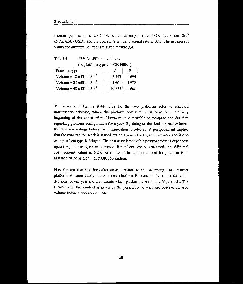
income per barrel is USD 14, which corresponds to NOK 572.3 per Sm3 (NOK 6.50 / USD), and the operator’s annual discount rate is 10%. The net present values for different volumes are given in table 3.4.
Tab. 3.4 NPV for different volumesand platform types. [NOK billion]
Platform type A BVolume = 12 million Sm3 2.243 1.694Volume = 24 million Sm3 5.961 5.972Volume = 48 million Sm3 10.235 11.600
The investment figures (table 3.3) for the two platforms refer to standard construction schemes, where the platform configuration is fixed from the very beginning of the construction. However, it is possible to postpone the decision regarding platform configuration for a year. By doing so the decision maker learns the reservoir volume before the configuration is selected. A postponement implies that the construction work is started out on a general basis, and that work specific to each platform type is delayed. The cost associated with a postponement is dependent upon the platform type that is chosen. If platform type A is selected, the additional cost (present value) is NOK 75 million. The additional cost for platform B is assumed twice as high, i.e., NOK 150 million.
Now the operator has three alternative decisions to choose among - to construct platform A immediately, to construct platform B immediately, or to delay the decision for one year and then decide which platform type to build (figure 3.1). The flexibility in this context is given by the possibility to wait and observe the true volume before a decision is made.
28

3. Flexibility
Platform A- 2.243 (12 million Sm3, p = 0.30)
^ Platform B
---- o
p = 0.30
"Wait" rYp = o.55 r{5= 0.15 1
-A—2.243 - 0.075 -B—1.694-0.150
-A—5.961 - 0.075 -B—5.972-0.150
-A— 10.235 - 0.075 -B—11.600-0.150
(12 million Sm3)
(24 million Sm3)
(48 million Sm3)
0 I
Fig. 3.1 Decision tree for the oil field development example. NPV figures are given in NOK billion.
First, consider a situation where the choice of platform type is based upon a given volume, typically the expected value. That is, the volume is treated as certain in the economic assessment. From table 3.4 we see that a volume of 24 million Sm3 should be developed by platform type B, which yields a NPV of NOK 5.972 billion. Since the uncertainty is “eliminated” through the expected value, the postponement alternative is clearly inferior. The optimal decision is therefore to fix the platform configuration from day one.
Assume now that the operator will get perfect knowledge (by some miracle ?) about the field volume after one year. The operator now acknowledges the uncertainty and wants to include it in the analysis. Due to the modest size of the problem it is straightforward to compute the expected NPV by hand. The results are given in table 3.5.
29

3. Flexibility
Tab. 3.5 NPV for different development strategies. [NOK billion]Strategy NPVImmediate constructionof type A 0.3 • 2.243 + 0.55 • 5.961 + 0.15 • 10.235 = 5.49Immediate constructionof type B 0.3 • 1.694 + 0.55 ■ 5.972 + 0.15 ■ 11.600 = 5.53Postpone decision 0.3 • max{2.243 -0.075, 1.694-0.15}
+ 0.55 • max{5.961 - 0.075, 5.972 - 0.15}+ 0.15 max{ 10.235 -0.075, 11.600-0.15} = 5.61
We still see that immediate construction of type B is better than immediate construction of type A. However, because of the revealed information after one year it is now optimal to postpone the decision until the volume is known. The gain from knowing the field volume thus more than offsets the additional construction costs. Hence, the net (expected) value of flexibility is NOK 80 million (NOK 5.61 - 5.53 billion).
Note that the rate of return used in the example is assumed independent of the risk. The discount rate is thus not modified as the operator gains perfect information about the volume. This corresponds to an assumption of the operator being risk neutral. However, if the initial rate of return (10%) is a risk adjusted rate of return (e.g., found by the CAPM), the discount rate should be adjusted to reflect the associated change in risk. The determination and updating of the discount rate will not be addressed in this context, and is clearly beyond the scope of the example. It is, however, important to be aware of the challenges involved when multi period projects with changing risk pattern are evaluated.
The simple example outlined above illustrates two important aspects of including uncertainty. First, it is clear that introduction of uncertainty as a distinct element in the analysis brings forward the value of flexible solutions. Without any uncertainty the “Wait and see” type of solution that turned out to be optimal in the example will never be preferred. Even though this may seem obvious, it should be noted that modelling of similar problems has to be given careful attention. As an example, consider an operator who uses the well known Monte Carlo simulation procedure to determine the optimal development strategy. Uncertainty is then included in the
30
3. Flexibility
analysis by solving the model several times, each time based on a field volume drawn from its probability distribution. Since each run of the model is a deterministic case, no value is given to flexible solutions such as the postponement decision described above. Hence, a simple simulation model would never pick the “Wait and see” solution.
Second, it is important to be aware of the fact that the flexible solution is (almost) never optimal in hindsight. (The “almost” can be omitted if, as is truly the case in most situations, flexibility has a cost associated with it.) By the time the field is depleted it is thus easy (with the achieved knowledge) to claim that one of the development plans with immediate fixation of platform type would have been a better choice. Fixing the platform type immediately to A, B and B, for field volumes of 12, 24 and 48 million Sm3 respectively, would all give a higher NPV than postponement of the decision. Therefore, choosing a flexible solution has not only a direct monetary cost associated with. It may also put some strain on the decision maker due to the element of belated wisdom.
3.3 Ty pes of f lexi bi lity
The example given above shows the value of one type of flexibility, that is, the possibility to wait until information about the true reservoir volume has arrived before the platform concept is decided. Since flexibility concerns the possibility to make future decisions, the option to wait is only one among several types of flexibility. Typically the variety of potential flexibilities in a project is closely linked to the complexity. Many alternative solutions and development strategies give a high number of flexibility types, while well defined and compact projects yield less flexibility types. The properties of an oil field development project therefore imply that several flexibility types are present.
Flexibility can conveniently be classified as either operating (managerial) flexibility or financial flexibility. This research addresses the former, i.e., the operating flexibility. As indicated by the term this flexibility is associated with possibilities for adjustments during the operation of a project. Operation is in this context given a broad interpretation, and should be conceived of as the entire period from the start to the termination of the project. This represents an expansion compared to the common interpretation, where the operation phase is regarded as the production
31

3. Flexibility
period of the field. Operating flexibility thus also includes e.g., the possibility to drill exploration wells and choose platform design, as well as options available during the production period.
Financial flexibility, on the other hand, concerns the options made available to the decision maker by the choice of capital structure. Even though financial flexibility is not a topic in this thesis, it is important to be aware of the sometimes close connection between financial and operating flexibility. For instance, assume that according to a separate analysis of operating flexibility the operator of an oil field has the possibility to delay the production. However, by postponing the production the cash flow is also postponed. A capital structure that requires a steady annual cash flow might then limit, or eliminate, the operating option to defer the production. An ideal evaluation of operating flexibility should therefore take into consideration the interactive effects between the two types of flexibility, in order to avoid sub-optimal solutions10. The effect of financial flexibility on operating flexibility, and vice versa, can be quite strong for large long term investment projects involving considerable uncertainty (Mason et al (1995)).
As stated, financial flexibility is omitted from this study. This may seem like a contradiction to the conclusion above, where emphasise is put on the importance of a combined assessment. The simplification is due to two aspects of the problem; the level of analysis and the focus on variables believed to be of major importance for the project value.
The main reason for the exclusion of financial flexibility is the scope of the research, which is flexibility at project level. In general, and for small fields in particular, the financing of a project is carried out at company level. For most oil companies the capital structure is therefore based on a portfolio of projects, and the cash flow from a single field is less critical for the overall performance. The connection between the operating flexibility of a small oil field development project and the capital structure (of the oil company) is thus likely to be moderate.
10 This interdependency can also be found between different types of operating flexibility, and has frequently been addressed under the term compound options (see e.g., Cortazar and Schwartz (1993), Geske (1979), Majd and Pindyck (1987), Pindyck (1991)). Put simply the assumption is that the exercise of one option, e.g., the investment in a platform, provide another option, e.g., the possibility to produce oil.
32

3. Flexibility
Based on the assumption of a moderate interdependency between the two flexibility classes it is further assumed that the financial flexibility is of minor importance to the value of the project. The segregation of the funding and operation of the project then makes it possible to analyse the value of operating flexibility on a separate basis. Any error introduced by this simplification is correspondingly regarded as insignificant to the general conclusions. In the remaining chapters of this thesis flexibility is thus conceived of as operating flexibility.
The possible operating flexibility of an oil field development project is discussed in the following sections, and concern four flexibility types. These are initiation flexibility, termination flexibility, start/stop flexibility and capacity flexibility.
3.3.1 Initiation flexibility
The possibility to decide when, or if, to start can be of great value to an oil field development project. For instance, consider a forthcoming change in relative costs. This could e.g., be due to a new arriving technology which improves the cost efficiency of well drilling. If the gain is of sufficient magnitude, it may be worth while to defer the start of the project in order to benefit from reduced development costs in the future.
The major gain from a postponement does however normally come from the benefit of getting new information. By being able to wait, the project can utilise information that arrives and take advantage of better knowledge. A widely used example is the possibility to wait and observe the oil price. Assuming the value of the operating project is a function of the oil price, this flexibility is similar to having an American call option11 written on the value of the project. In the terminology of financial options the investment cost of the project is the exercise price of the option, while the last possible time to start the project is the option’s expiration date. Instead of using a positive NPV as criterion for project initiation, the decision rule is now to defer the start until the oil price has reached a given level (above the break even price).
Figure 3.2 illustrates the value of initiation flexibility. The straight line gives the value of a project without the possibility to wait, while the two curves shows the values of a project if the initiation can be deferred. For simplicity it is assumed that *
" See Hull (1993) for an introductoin.
33

3. Flexibility
the value of an operating project is proportional to the oil price, which follows a geometric Brownian motion given by equation (3.1). (The geometric Brownian motion and its properties are discussed in chapter 6.)
= adt + adz (3.1)
where P is the oil price a is the drift rate t is the timect is the variance parameterdz is the increment of a Wiener process
First, consider a project without any initiation flexibility. The decision to start must be made now, and from the figure P* is the critical price. If the current oil price is below P* the project is not initiated. A price above P yields a positive value and, hence, implies that it is optimal to start the project. This analysis represents the traditional NPV procedure, where the decision criterion is a positive NPV. P* is thus the break even price.
Assume now that the decision maker can wait for some time before he decides whether to start the project or not. This situation is depicted by the two curves, which give the value of a project with initiation flexibility for two different variance parameters, and <j2 (o) < (%). The figure reveals three important effects of including initiation flexibility.
First, it is evident that the value of a project with flexibility is always higher or equal to the value of a project without flexibility12. This is a general property of flexibility, and is not limited to initiation flexibility. Second, the value increases with increasing volatility. Since the decision maker is free to decide if the project should be initiated or not, the value of the option (to start the project) has a lower bound of zero. The effect of the bound is similar to having an insurance against unfavourable outcomes. However, the decision maker can still take advantage of future price increases. A higher variance of the future oil price thus increases the upside potential, but does not have a parallel influence on the downside. As a result the value of initiation
12 The valuation does not take into account the cost of obtaining the flexibility. Alternatively can the cost be assumed sunk.
34

3. Flexibility
flexibility is high if the variance parameter is high, and vice versa. Third, the existence of initiation flexibility implies that the simple NPV value rule, which says that the project should be started as long as P > P*, is no longer valid. The decision maker’s possibility to wait is of value, and an initiation of the project represents a loss of this value. An immediate start thus involves a higher cost to the operator, and the required price for an immediate initiation therefore increases to Pi and P2 for variance parameters equal to <7/ and a2, respectively. Thus using the NPV method to compare projects where differences in initiation flexibility is significant would support wrong decisions and could involve gross errors.
Oil price
Fig. 3.2 Value of project with/without initiation flexibility. The straight solid line gives the value if there is no flexibility. The curves are the values with flexibility, oj < <j2.
A study by Paddock, Siegel and Smith (1988) reveals that the option to wait can represent a significant part of the value of leases on offshore petroleum tracts. Bjerksund and Ekem (1988) obtain similar results, based on an analysis of investment and production profiles submitted by the Norwegian Ministry of Oil and Energy. They define the flexibility factor as the value of the project if the initiation can be deferred infinitely divided by the value if the project were initiated immediately. For the analysed project the flexibility factor is 2.39. In a more recent
35

3. Flexibility
study (Bjerksund and Ekem (1990)) they report values ranging from 0.02 to 4.84, though using artificial data.
Initiation flexibility is not restricted to a flexible start-up time of the project, but can also be related to work tasks in the project. Consider for instance a development project consisting of four phases; exploration, platform design/construction, production well drilling and oil production. After the platform is constructed it still may be possible to defer the drilling of production wells. This option is another example of initiation flexibility, where the drilling can be conceived of as a separate project. Also the flexibility in the example given in section 3.2.3 falls within the class of initiation flexibility. Here the completion of the platform is treated as a separate task, and the value of flexibility is present because the decision maker can wait one year before he makes the decision.
3.3.2 Termination flexibility
The option to terminate is another flexibility type that is present in a field development project. Traditional capital budgeting procedures like the NPV method typically presume that the project duration will coincide with the expected lifetime. However, it may not be optimal to continue operation if events, either internal or external, with a negative impact on the project occur. The value of being able to terminate can then be substantial, in particular for projects with a long expected remaining lifetime.
For a field development project the option to terminate can, at least theoretically, be exercised in any project phase. However, governmental regulations and lease obligations may restrict the oil company’s freedom of action. For instance can an awarded exploration lease require that a predetermined exploration programme is carried out. If this is the case the oil company does not have the opportunity to terminate the project until it has fulfilled its obligations.
As the development project evolves the value of the termination flexibility declines. This is similar to the well known results for financial options, where the value of the option decreases as the time to expiration (the maturity date) approaches. For the development project the remaining life time corresponds to the time to expiration.
36

3. Flexibility
Due to the cash flow profile, the reduction in the value of termination flexibility as time passes is more distinctive for an oil field development project than for most projects. Substantial investments during early periods of the project implies that the positive cash flow comes late (figure 3.3). As a consequence the exercise price, i.e., the cost of termination, makes a steep rise when the investments are completed. The rise in exercise price makes it less likely that the option to abandon the field is utilised. Hence, the value of the flexibility is reduced.
Production-Expl. Dev.
Fig. 3.3 Generalised outline of cumulative cash flow for an oil field development project. (Expl.: exploration, Dev.: field development (infrastructure, platform construction, well completion etc.))
The value of termination flexibility in an oil production project is analysed by Stensland and Tjpstheim (1991). In their analysis the production profile is assumed uncertain, and four different models for reduction in uncertainty are considered. The value of flexibility is measured by the ratio of the NPV with termination flexibility to the NPV for the deterministic case. The ratio is given as a function of the uncertainty resolution model and the operating cost of the field. As expected, the value of the termination flexibility increases with increasing operating cost. For an artificial data set with close resemblance to a practical case the ratio range from 1
37

3. Flexibility
(operating cost is zero) to 1.6. Calculations made for the Draugen field13 yield ratios
in the range of 1.3 - 1.4, depending on whether a fixed or movable platform is chosen. This corresponds to a rise in expected net present value of more than NOK 1 billion to NOK 3.9 billion for the movable alternative.
3.3.3 Start/stop flexibility
In addition to the choice of when to initiate and terminate the project, the possibility of starting and stopping the project during its operation can be of significant value. A normal assumption underlying traditional capital budgeting procedures is that the project operates in each year of its life time. However, especially for projects with variable operating costs this might not be optimal, since the revenue can fall below the variable cost for a period of time. Recognition of this type of flexibility is therefore important when projects with different ratios of variable to fixed costs are compared.
The value of start/stop flexibility is not limited to cases where the project is shut down only in order to avoid negative contribution margins. As for the initiation flexibility, the start/stop option represents an opportunity to wait before a decision is made. The decision is in this context the restart of the project. By waiting the decision maker can take advantage of arriving information, or benefit from favourable future conditions.
In an oil field development project the possibility to start and stop the project can exist at several stages. At an aggregate level the start/stop option can be conceived of as an opportunity to schedule the phases. For instance, stopping the project temporarily after the exploration phase is completed implies a postponement of the next phase (normally choice of development concept.). At a more detailed level the option yields possibilities for progress adjustments. However, for a field development project the cost of starting and stopping the project can be high, making the flexibility less valuable. In particular this might be the case when the field has been put in production.
The latter case is analysed by Brennan and Schwartz (1985), who value start/stop flexibility in a natural resource development project. Under the assumption of a
13 The Draugen field was discovered in 1984. Estimated recoverable reserves are 94.5 million Sm3 oil and 5.4 billion Sm3 gas (NOE (1996)).
38

3. Flexibility
stochastic (geometric Brownian motion) output price they develop a general valuation model for the development project, in which the exploitation can be started and stopped. It is also possible to terminate the project. Even though it is straightforward to solve the model numerically it does not, in general, provide an analytical solution. In order to obtain a tractable model the general version is simplified. The main modifications are as follows. It is assumed that the physical inventory of the resource is infinite. Further, it is assumed that the maintenance cost for a shut down project is zero. Termination of the project will thus never be optimal. And, finally, the exploitation rate (when operating) is assumed fixed14.
Given these assumptions the value of the project can be illustrated by figure 3.4.
operating
shut down
Output price
Fig. 3.4 Value of project when operating (V„peratlng) and shut down (Vshut down).Cstan is the cost of starting, and Cstop is the cost of stopping the project. Source: Brennan and Schwartz (1985).
In the figure the dotted line gives the value of the development project without start/stop flexibility. The result points to two important properties of the start/stop flexibility. First, since the value of flexibility is given by the difference in project value with flexibility (solid line) and without flexibility (dotted line), we observe that the value of flexibility diminishes as the output price increases. The intuitive
14 In the general model the rate was costlessly variable between an upper and a lower bound.
39

3. Flexibility
explanation is that a high output price makes it less profitable to close down the project. The option to start/stop the project will then seldom be used, and its value is correspondingly low. Second, it can be shown that as the cost of stopping the project (Cstop) goes to infinity the value of the operating project approaches the value of a project without the start/stop flexibility. The reason is similar to the previous explanation. A high stopping cost makes it less likely that the option will be exercised.
The ability to temporarily stop the project represents a generalisation of the initiation flexibility and the termination flexibility discussed in previous sections. If there is no restrictions on the time the project is shut down, the initiation of the project can be regarded as the first restart. The “temporary” stop then corresponds to the time since the project could first start. Termination of the project can, in a similar way, be interpreted as a “temporary” shut down of infinite length.
Even if it is possible to include the initiation and termination flexibility in the start/stop class, a separate discussion is convenient in most cases. For instance can a project contain initiation flexibility, but, once started, it must be operating continuously during its lifetime. Similar differences between start/stop flexibility and termination can exist. Another property that typically differs is the fixed costs which incur while the project is stopped. Termination of the project usually eliminates these costs.
3.3.4 Capacity flexibility
Section 3.3.1 to 3.3.3 discuss the possibility to influence the progress by starting and/or stopping the project. Capacity adjustment yields another type of flexibility, in the sense that it offers a possibility for modifications without directly affecting the operation schedule for the project. However, the indirect effects might be of a similar nature.
Capacity in an oil field development project can be related to various fields. For instance are administrative capacity, investment capacity, maintenance capacity and transport capacity all relevant, and of value to the project. However, in this research focus is on managerial flexibility, i.e., the ability to affect the course of a project by acting in response to resolution of uncertainty over time. Capacity required to carry
40

3. Flexibility
out the control actions, e.g., administrative capacity, is therefore not addressed in this context.
Capacity flexibility is often conceived of as the possibility to expand or contract the scale of the project. Typically this flexibility is of a sequential nature, where e.g., one expansion renders possible another expansion. The similarity to so-called compound options, i.e., options on options, should be obvious. For a general project the expansion or contraction of scale can be achieved by making adjustments along three axes, as illustrated in figure 3.5. Of these, only two are relevant to an oil field development project. This is the possibility to change the output/activity level, and the option to extend or shorten the production period/project duration. A change of the product/activity mix is not an option, in the sense that the product is fixed through the physical properties of the reservoir fluid.
output /activity level
product / activity mix production period /
project duration
Fig. 3.5 Expansion/contraction of the scale of the project.
The possibility to adjust the activity level of a development project depends on the project stage. For instance, in the exploration phase the activity can be boosted by drilling more, or perhaps deeper, wells within the same time period. Capacity flexibility in this context is the possibility to adapt the drilling programme to future changes. During the construction of the platform the capacity flexibility is given by the decision maker’s option to alter the construction schedule. Assuming the platform is build by contractors, this possibility is probably modest.
41

3. Flexibility
The typical flexibility concerning activity level is the possibility to change the production level, i.e., the depletion rate of the reservoir. Normally the uncertainty surrounding the reservoir is high. This implies that neither the effective well rates nor the total volume of the reservoir are known with certainty. Correspondingly, the production and processing capacity of the platform should be designed to facilitate future adjustments as a consequence of changes in reservoir conditions. For instance, if the true reservoir volume is higher than expected the operator may choose to increase the annual production. In order to achieve this the platform must have capacity flexibility to handle the additional through-put. Free space on the platform deck for installation of new separators is an example of such flexibility.
The second capacity flexibility available is the possibility to extend (or shorten) the project duration. As for the activity level the possibility to make adjustments is connected to the stage of the project, but is typically related to the production period. A shorter (longer) production period can be achieved by an increased (decreased) production rate (ceteris paribus). Hence, the flexibility to change the output level and the effective production period are closely related. The purpose of a higher production level is normally to increase the NPV by an accelerated sale, but a raise might for instance be due,to upcoming opportunities at other fields. Alternative use of the platform will increase the alternative cost, and can make it profitable to relocate the platform before the scheduled project termination.
The flexibility to extend the production can be of value if restrictions, e.g. of the platform, makes it impossible to deplete the reservoir within the expected lifetime of the project. An extension of the production period may then be required to take advantage of an increase in the recoverable field volume.
Both the value of an optional change in project duration and activity level can be analysed by procedures similar to those referred to in previous sections. For instance can the possibility to extend the production period be treated as a separate option written on the additional production period. A similar approach can be used to find the value of activity level flexibility, as illustrated by Triantis and Hodder (1990). They develop a model for valuation of flexible production systems by using a portfolio of European options. For a hypothetical example they show that capacity flexibility can be of substantial value. This is in line with the results of Brennan and
42

3. Flexibility
Schwartz (1985), whose model can be considered a special case of the more general model by Triantis and Hodder.
3.4 Evaluation of flexibility
3.4.1 Analyses of flexibility and its value
Several contributions address the value of flexibility in projects related to oil field development. In particular the use of contingent claims analysis has shown promising results, and the literature provides many examples where the value of flexibility is evaluated by this method. The contributions referred to in the previous section represent a sample of such studies. A common trait of the analyses is their focus on a single type of flexibility, often under the assumption of the oil price as the only uncertain variable. Studies were several types of flexibility are included are somewhat harder to find.
In the discussion of the different types of flexibility it is stressed that each can be of substantial value to the project. However, the question of which flexibility type that adds most value to the project is not answered, and, on a general basis, this is not possible. Since the value of flexibility is closely related to uncertainty and how it is revealed, the gain from different flexibility types will depend on parameters and properties specific to the project. A flexibility type of great value to one project might thus be, at least theoretically, insignificant to another project.
The few analyses that perform a combined assessment of several flexibility types yield no decisive conclusions regarding the value of one flexibility type compared to another. Bjprstad et al (1989) and Tennfjord (1990) use similar models to evaluate flexibility, based on an artificial data set and data related to the Ula field, respectively. In both studies the simultaneous presence of initiation and termination flexibility is shown to be significant, but a separate evaluation is not carried out. Bjerksund and Ekem (1990) starts out with initiation flexibility, and then adds termination flexibility or start/stop flexibility. They conclude that the effect of adding another flexibility type to the model is negligible, and that the major difference in project value is found in going from the traditional NPV approach to a model with initiation flexibility. However, it is not possible to draw the general conclusion of initiation flexibility being dominant, since the value of different
43

3, Flexibility
flexibility types in general is not additive. If the initiation flexibility was added to one of the other flexibilities the result might thus be different.
3.4.2 Combining flexibility types
The missing additive property of value of flexibility can be explained by the following observation. Consider first a project with either initiation, termination or start/stop flexibility. As stated previously the value of flexibility is related to the options it provides to reduce the effect of undesired outcomes, e.g., negative net sales income. Flexibility can thus be conceived of as an insurance, which limits the downside risk. By including one type of flexibility the project is therefore hedged against some events with negative impact on the project’s performance. (If the project is depicted by a decision three the flexibility cuts off branches in the three with inferior expected value.)
Now, assume that another flexibility type is added to the project. For instance can the project have both initiation and termination flexibility. As for the “first” flexibility type present in the project, the added flexibility increases the value of the project by letting the decision maker take measures to reduce undesired effects of future events. However, the introduction of the first flexibility type has already limited the downside risk. If the two flexibility types affect some common scenarios it is thus likely that the insurance provided by the second flexibility is partially covered by the first flexibility. Adding additional flexibility to a project has therefore in most cases less value than if the flexibility was added to a project without any flexibility. Appendix A illustrates the effect by a simple example, where initiation and termination flexibility is combined. Similar effects are also identified in chapter 8.
Additivity of value of flexibility is nor the case for capacity flexibility. But, while initiation, termination and start/stop flexibility controls the schedule of the project, capacity flexibility affects the scale. As a consequence, adding another flexibility type may either reduce or increase the value of the capacity flexibility. Consider for example a project where the terminal pay out depends on the price of a produced product. With three possible prices the pay outs are given in figure 3.6. The numbers are per produced unit, and p denotes probability. Hence, the probabilities are 0.25, 0.5 and 0.25 for a pay out of 4,2 and -4, respectively.
44

3. Flexibility
p = 0.25
p = 0.50
p = 0.25
Fig. 3.6 Terminal pay out per produced unit.
Assuming that only one unit is produced, the expected value of the terminal pay out without any flexibility is 1. Two types of flexibility are now introduced - termination flexibility and capacity flexibility. With termination flexibility the decision maker has the option to stop the project (at no cost) if the terminal pay out becomes negative. Capacity flexibility in this context gives the decision maker a possibility to expand or reduce the production by a factor X before the terminal pay out per unit is revealed. Table 3.6 summarises the value of flexibility for different cases.
Tab. 3.6 Expected value of flexibility.Flexibility Expected value of
terminal pay outExpected value of flexibility
No flexibility 1 -Termination flexibility 2 ICapacity flexibility X X- 1Termination and capacity flexibility 2-X 2-X - 1
From the table it is evident that the value of flexibility is not additive. If the capacity flexibility implies an option to expand the production, i.e., X > 1, the value of this flexibility increases if combined with the termination flexibility
45

3. Flexibility
X> 1W (3.2)
(2 %-!)-!> X-l
The left hand side in equation (3.2) is the increase in expected value if capacity flexibility is added to termination flexibility, while the right hand side is the value of capacity flexibility by itself. If the capacity flexibility only gives the decision maker a possibility to reduce the production (%< 1), the flexibility will be of no value (regardless of whether it is evaluated as a stand-alone flexibility or in combination with termination flexibility). The result follows from the fact that an option to reduce the production will never be exercised.
3.5 Concluding remarks
As revealed by the example above and appendix A, a comparison of different flexibility types with respect to their value should be linked to the underlying project. General guidelines for priorities between flexibility types are thus hard to obtain. The fact that value of flexibility does not have an additive property implies that investment in flexibility requires a unified evaluation in order to avoid sub- optimal solutions. Assuming the decision maker can invest in several types of flexibility the investment problem bear resemblance to a portfolio management problem. That is, the decision maker’s challenge is to construct an optimal portfolio of flexibility.
Due to the complexity of an oil field development project and the combining effect of the value of flexibility this problem is not solvable by hand. The non-additive property of the value of flexibility thus further strengthens the demand for a DSS for evaluation purposes. Failing to take this property into account may result in wrong decisions and a reduced project performance. Thus a comparison of flexibility should not be done by use of separate studies, but as a unified analysis including the relevant flexibility types.
46

4. Modelling the offshore oil field development project
4 MODELLING THE OFFSHORE OIL FIELD DEVELOPMENT PROJECT
With an investment level of several billions, a project duration of decades and a high complexity, the need for methodology and tools to support decisions regarding development strategy and platform configuration is obvious. The applicability of such tools is essentially determined by their ability to handle huge amount of data. Since a complete field development model by far outgrows today’s computing power, the solution is typically a trade off between conflicting goals.
The construction of such a model is not straightforward. In this chapter the modelling issue is discussed, together with an assessment of different solution methods. The discussion leads to a simplified description of the oil field development project.
4.1 Introduction
Mathematical models are used frequently in society to explain system behaviour, and serve a wide variety of purposes such as macroeconomic planning, production planning, weather forecasting etc. Colloquially, a model is conceived of as something that mimics relevant features of the situation being studied (cf. Murthy et al (1990)). Even though this notion of a model is sufficient in many cases, it is helpful for the further discussion to give a more precise definition. The following definition is given by Bender (1991), and is suitable for this thesis.
« A mathematical model is an abstract, simplified, mathematical construct related to a part of reality and created for a particular purposes
Modelling complex systems like an oil field development project involves many challenges, and modelling is often regarded to be an art (see e.g., Cross and Moscardini (1985)). The main objective is (of course) to obtain an adequate representation of the underlying problem. However, additional objectives like solution time and model size are often conflicting goals which inevitably forces the modeller to make trade offs between the level of detail and implementability. Even though this may seem as a nuisance it, in fact, points to the core issue of modelling.
47

4. Modelling the offshore oil field development project
A model is, and should be, nothing more than an acceptable description of the real world. This necessarily implies that only the main features of the real problem can be captured. The high complexity of a field development project thus requires that some elements are treated roughly in order to get a solvable model.
The development of a petroleum field is a project which involves several disciplines, including geology, engineering and economics. However, the project team is not a static unit, and as the project develops the structure of the project organisation changes. As a result the resources provided by different professions vary over the project’s life cycle, and at times only a single discipline may be involved. But, even though the manning of the project varies the project is clearly an interdisciplinary task.
One consequence of the interdisciplinary property is that the models applied within the project differ substantially with respect to level of detail and complexity. As briefly discussed in chapter 2, the emphasis has been put on technology related models, while the economic assessment is made by relatively simple models. A common trait among such models is that uncertainty has not been an integrated part. Especially if the technology related models are considered this statement is valid. Many of these models require extensive information and provide detailed output under the assumption of perfect knowledge (cf. Bjprkvoll and Lund (1995)). Typically the high level of detail is made possible by the very assumption of complete certainty. This level of detail is impossible to transform into a universal model with uncertainty. A major challenge when modelling the field development project is therefore to condense the description.
The development project can conveniently be seen as a sequential problem with a finite number of phases. It thus seems natural to divide the project into stages to reflect the sequential pattern of decisions and the uncertainty characteristics at different levels. Several studies have proposed different ways of phasing, reflecting the objective of the analysis. The classification given here (figure 4.1) is based on Klitz (1980) and Rolstadas (1986). It divides the development into 10 phases, starting with the awarding of the licence and ending when the project is terminated. This description is too detailed for our purpose, but serves as a convenient starting point for a simpler model. Note that the licensee is not obliged to complete the project once it is undertaken. Hence, termination can occur at all stages of the project and does not necessarily follow the production phase as indicated by the figure.
48

4, Modelling the offshore oil field development project
ConcessionSeismicsurvey
Explorationdrilling
Feasibilitystudy
Conceptualstudy
EngineeringConstruc
tionInstallation Production -| Termination
v_ _ _ _ _ _ _ _ _ J
Fig. 4.1 Phases of a petroleum field development project.
For all models the formulation is, more or less, influenced by the solution technique. The maybe most obvious example is the connection between a discrete solution procedure and the possible variable values. Consequently, a discussion of the model should be related to an assessment of the solution method. To provide a foundation for the following model description, alternative methods are discussed in this chapter.
4.2 Going from a deterministic to a stochastic model
In a deterministic world, the decision maker has all the advantages of perfect foresight. He knows what will happen, when it will happen and what consequences his actions will have. This has normally been the context in which oil field development projects have been evaluated during the last decades, and has been the foundation for most DSS’s. By including uncertainty, the picture becomes more blurred and makes greater demands on the evaluation procedure, both regarding the model input and, more important, the modelling issue itself. The increased demand for data and computing power that accompanies the introduction of stochasticity inevitably makes the model more complex. As will become evident in later chapters, this is also the case for this study.
As mentioned previously, the transition from a deterministic to a stochastic model gives value to flexibility. While flexibility is of no value in a deterministic world it may be of great importance when uncertainty becomes a part of the evaluation task. Unfortunately flexibility usually has an associated cost15. Different kinds of flexibility require different investments, and the decision must balance the increased
15 If the flexibility was free the problem would degenerate, and it would always be optimal to choose the development strategy with flexibility instead of the one without any flexibility.
49

4. Modelling the offshore oil field development project
investments against the expected revenue. The reason for choosing a flexible solution is of course that the expected gain outweighs its costs. However, in retrospect, when all uncertainty has been revealed, the flexible solution never turns out to be the optimal one compared to a fixed, tailor-made alternative (see section 3.2.3). This means that the transformation from a deterministic model to a stochastic model increases the possibility of criticism based on hindsight.
One might argue that the possibility of a fixed (non-flexible) solution being optimal in retrospect in most cases is small and, hence, that the chance of some criticism based on hindsight always exists. This might be the case, but does not alter the fact that when looking back, the flexible solution is always inferior to some other development strategy. Choosing such a solution is therefore equivalent to forfeiting the possibility of achieving the best obtainable development. Even though this aspect can be viewed as irrelevant to the modelling task itself, it may have an impact on the implementation of stochastic models in companies.
As uncertainty is introduced in a model, the scheduling of events and decisions becomes more crucial. The value of flexibility is linked to the ability to act based on available knowledge at a given time. Correct sequencing of information arrival vs. decisions is therefore important to obtain a good model. Perhaps the most important pitfall to avoid, is to make the model inconsistent. This could for instance happen if the formulation provides the decision maker in the model with more (or less) information than actually available. Typically, this is a problem that may arise for large and complex models composed of several elements linked together.
4,3 Some modelling considerations
Design of a model requires that careful attention is paid to many, often divergent, features. Depending on the purpose of the model, emphasis is put on different elements, but the overall objective is on all occasions to obtain a reasonable description of the real problem.
It is outside the scope of this thesis to delve deeply into the field of model building. A thorough study of the various aspects related to the design and construction of a model could probably be the subject for several separate research projects. In spite of this it seems logical to present a broad overview of some main issues of modelling,
50

4. Modelling the offshore oil field development project
thereby to provide a background for the following exposition. Two considerations are here of particular interest; how to obtain a simple problem description, and what kind of solution is requested.
4.3.1 Simplifying the problem description
Since a model, at best, is an adequate description of a complex reality, some aspects of the real world problem are typically not considered. Thus the model is a simplified problem. Several approaches can be taken to obtain this compact problem description. Here measures related to the variables and the time horizon are addressed. These are commonly regarded as the main driving forces towards a large and computationally demanding model. (A large set of parameters increases the size as well, but is usually much easier to handle.) Once more it is stressed that modelling and simplification of the problem is closely connected to the solution technique, and a general discussion as provided here can not be used to consider the efficiency of the different approaches.
Variables.
The variables of an oil field development project are numerous, and the proportion that can be captured in a unified model is correspondingly small. A reduction in the number of variables can be obtained in two ways, of which the elimination of variables is the most evident. Typically this implies that a few variables are modelled, while the remaining either are omitted or represented by their expected value. An elimination of variables in line with this is simple, in the sense that variables included in the model are identical to the original ones. However, this somewhat coarse approach may not be satisfactory, as the modelled variables tend to be few, but very detailed. Their ability to mirror the real problem can thereby be limited.
Usually a more suitable approach is to aggregate variables, or to construct proxy variables, to capture the essence of the problem. Each variable then synthesise a set of underlying elements. For instance, consider the modelling of an oil reservoir. Instead of making the volume a function of variables such as porosity, permeability, saturation etc., the volume is the variable itself. The advantage is that main elements are focused upon, allowing the model to directly address the aggregate variables believed to be of great importance. Nevertheless, the challenge of finding a good formulation still persists.
51

4. Modelling the offshore oil field development project
The selection of model variables also involves a selection of formulation. At an aggregate level this means a choice between a deterministic and a stochastic representation. As pointed to earlier, a stochastic formulation is generally more demanding, both regarding input and the required modelling of information resolution. The selected stochastic variables should therefore be significant and probably relatively few. Figure 4.2 illustrates the screening of variables made as part of the model building.
Some Eliminate/filter "Perceived aggregate "Simplified
problem' description''Real world'
Determ.variable
Variable 3 r
Stoch.variable- Variable 5
Variable 1 Variable 1
Variable 2
Variable 3
Variable 4 Variable 4
Variable 6
Variable 5
Variable 1
Variable 4/5
Fig. 4.2 Screening of variables to simplify the problem description.
Time horizon.
The development and depletion of an oil field may last several decades. Since uncertainty increases over time a long horizon inevitably makes it harder to forecast the performance of the field. As a result the evaluation task becomes more difficult. By using a large time frame the model also covers more decision points. Ceteris paribus this enhances the computational effort required to solve the problem (assuming the decisions are relevant to the model).
The intuitive approach to avoid the problems associated with a large time span is simply to limit the horizon of the analysis. This implies the need for specification of
52

4. Modelling the offshore oil field development project
terminal values, which should reflect the value of a continuing project. For long term projects the error introduced by this simplification is usually minor, since the discounting effect makes remote events less important for the present value. Following this chain of thought an increasing discount factor makes the approximation more acceptable. For instance, the NPV of one USD received in 2017 is today (1997) 38 cents if the annual rate of return is 5 percent. With an annual rate of return of 15 percent its value is reduced to 6 cents. There is of course no given answer to where a reasonable limit should be set. However, as the analysis horizon decreases, specification of the terminal values in most cases becomes harder. A short horizon is thus computationally attractive, but also induces assessment problems.
Complex problems like a development project commonly require numerical solution procedures. The problems arising in discrete models are thus of particular interest in this context. If the model is discrete in time the number of periods increases as the time horizon gets longer. One way to solve this is to adjust the length of each period accordingly, thereby to keep the number of periods constant. Another approach is to let the period length increase over time. That is, the imminent periods are short while more remote periods are of longer duration. The reasoning behind a more coarse division as we move into the future is, as above, the rising uncertainty and declining effect on the present value.
Both approaches are examples of time aggregation, and the common idea is to limit the number of planning periods to obtain a more manageable problem. Time aggregation is often an appealing way to simplify the problem, but must be used carefully. Typically the solution to the aggregate problem is different from the solution to the original problem (Haugen (1991)).
Finally, an opposite solution to the problem of large time spans should be mentioned. Even though not applicable to all solution methods, an infinite horizon may ease the computational burden significantly. The infinite horizon implies that the time scale is removed from the problem. Thus, ceteris paribus, the decision maker faces the same problem tomorrow as today. Given this the problem is simplified and can usually be solved more efficiently. For an oil field development project the assumption of an infinite time horizon does not conform to Norwegian regulations, which require depletion of the field within a given period of time. Hence, the error introduced by this approximation must be balanced against the associated computational advantage.
53

4. Modelling the offshore oil field development project
4.3.2 Requirements to the solution method
The purpose of the model is to improve the foundation for decision making under uncertainty. By running the model the decision maker should enhance his understanding of the problem, thereby obtaining a better basis for assessment of the alternative development strategies. These are general requirements and can, more or less, be fulfilled by various decision support systems. However, the main goal is to provide a model that addresses flexibility and its value in a rational manner. Thus the ability to capture the decision and information structure of the problem is crucial.
Generally, problem solving by mathematical techniques is done by either simulation or optimisation techniques. As pointed to in chapter 3 the traditional Monte Carlo simulation approach does not give due attention to flexibility, and a viable method that amends this deficiency is hard to see. Use of simulation techniques is therefore considered inadequate in this context. Apart from the apparent drawback of not handling flexibility in a satisfactory way, the solution offered by a simulation method usually differs from analysis to analysis. Unless the simulations are made with identical sets of input data, the results will change between model runs. Typically this is the case when stochastic variables are involved. For consistent decision making this can be undesirable, since the decision basis may depend on the solution procedure (for instance the number of model runs in a Monte Carlo simulation).
The second class, optimisation methods, represent a different approach to mathematical problem solving. Instead of a synthesis of several model runs, the optimisation techniques compute one optimal solution. The dependency on the solution procedure is in this respect thus not as high as; for simulation techniques. Among the optimisation techniques several are well capable of handling uncertainty and flexibility. Hence, considering the objective of the model, this research is based on optimisation methods for the evaluation purpose. As shown below, these methods may also have the benefit of providing a complete strategy, as compared to a single initial decision. This gives the decision maker a better basis for evaluation and the follow up of projects. To be fair, it should be mentioned that the associated advantages of an optimisation method do not come free of charge. Typically the cost is a computationally more demanding model. This topic is addressed in subsequent chapters.
54

4. Modelling the offshore oil field development project
4.4 Alternative methods
As a consequence of the broad scope of the outlined framework, the evaluation model touches upon many subjects of economical or technological nature. The wide area of topics implies a comprehensive existing literature and several approaches can be found that deals with related problems. In particular contributions related to technological issues of oil production are numerous. Since an in depth analysis of each element inevitably becomes unmanageable in a model, this thesis focuses on the value of flexibility at an aggregate level. Hence, the appropriate approach should stress the decision structure and the development of the knowledge base as the project evolves.
4.4.1 Foundation and terminology
Three approaches have been considered in this research; contingent claims analysis (CCA), dynamic programming and scenario aggregation. Even though these mathematical tools are referred to as alternative methods, it is important to be aware of the difference in foundation. Both dynamic programming and scenario aggregation can be classified as decision analysis techniques, and are general tools for solving sequential problems. As such they can be applied to a wide variety of problems, and either provide a procedure for project evaluation under uncertainty. CCA builds on financial theory, and is often regarded synonymous to options theory. As opposed to dynamic programming and scenario aggregation the CCA technique makes assumptions of the market, and represents economic theory. (See e.g. Dixit and Pindyck (1994), p. 93-94, for further elaboration on this topic.) In spite of this difference, it is common in the literature to consider the techniques as alternatives. This procedure is adopted in the following.
The following sections discuss the suitability of CCA, dynamic programming and scenario aggregation to value flexibility in offshore oil field development projects. Dynamic programming is in the literature used to solve both deterministic and stochastic problems. In this context the uncertainty aspect is decisive. Thus to distinguish the approach from its deterministic counterpart it will hereafter be referred to as stochastic dynamic programming (SDP).
55

4. Modelling the offshore oil field development project
4.4.2 Contingent claims analysis
Option pricing theory and, in general, contingent claims analysis, offers an efficient framework for the valuation of corporate assets and liabilities, and has thus gained much popularity over the recent years. Since the seminal papers by Black and Scholes (1973) and Merton (1973) was presented in 1973, application of option pricing theory for evaluation of financial investments has increased rapidly. While originally designed to evaluate traded securities, the approach has during the last decade found a field of application within real investments (so-called real options). Allowing for a "reinterpretation" of the investment possibility at hand, many investment opportunities involving flexibility may be regarded as projects offering options to the decision maker. Option pricing theory then provides an elegant evaluation of projects yielding this kind of flexibility, and examples of such in the literature are abundant. (For contributions related to oil field development projects see e.g., Bjerksund and Ekem (1990), Ekem (1988), McDonald and Siegel (1986), Paddock, Siegel and Smith (1988), Pickles and Smith (1993) and Pindyck (1980).)
Option pricing theory is based upon arbitrage theory. By assuming the existence of spanning assets (cf. Dixit and Pindyck (1994), p. 117) it is possible to apply the risk neutral evaluation principle. This is also known as the “complete markets” assumption, and ensures that an investor is able to perfectly hedge every project risk by trading existing securities. The question of whether such spanning assets16 can be found or not is thus the crucial factor in this context. To answer this question the close relationship between relevant risk and the level of analysis must be addressed.
Among contributions that apply real options, most consider problems with a single stochastic variable. For those considering oil field development projects, this variable is, with few exceptions17, the oil price. The focus on a single stochastic variable can be justified by an assumption of a highly diversified investor, which makes market risk the only relevant risk. Other uncertain quantities are thus assumed to vary in an unsystematic way, and, hence, can be avoided through diversification.
The classification of relevant vs. irrelevant risk depends on the level of analysis. An example of possible levels for an oil development project is given by Bphren and
16 The spanning asset(s) may either be a single asset or a (continuously adjusted) portfolio of assets.17 See e.g., Paddock, Siegel and Smith (1988) who models the value of a developed reserve as a stochastic process.
56

4. Modelling the offshore oil field development project
Ekem (1985), who identify six levels (figure 4.3). The arrow indicates increased level of diversifiable risk. An analysis made at project level thus has the highest number of non-diversifiable risk categories. These would typically cover most, if not all, of the uncertainty surrounding the development project. Correspondingly would an analysis carried out at community level have only a few non-diversifiable risk categories.
The project
The company
The government income from the trade considered
The trade
A community's portfolio diversified at national level
A community's portfolio diversified at international level
Fig. 4.3 Investment analysis levels.
To assume that the market risk, e.g., the oil price, is the only relevant risk category complies with an analysis at community level. This is reasonable, since the community possesses a well diversified portfolio. However, the level of analysis taken here corresponds to the project level in figure 4.3. In this case the relevant uncertainty in the simplified project description is not merely represented by the oil price, but cover also event uncertainty18 in the form of e.g., an uncertain well rate. The properties of these elements are of such nature that it seems highly unlikely that the stochasticity can be mirrored by marketed assets. For instance, a jump in the well rate would not be reflected in the value of any traded asset. Nor is it possible to construct a portfolio of assets with the requested property. In its pure form options
18 The terminology is adopted from Hirshleifer and Riley (1979) who define event uncertainty as uncertainty related to the exogenous data of the economic system. (Its endogenous counterpart, e.g., the oil price, is termed market risk.)
57

4. Modelling the offshore oil field development project
theory is therefore not an adequate approach to value flexibility when uncertainty surrounding the reservoir is a main element.
The conclusion given above is also reflected by the fact that contributions that apply option pricing theory to evaluate problems with event uncertainty are scarce. Nevertheless, some work has been done based on the assumption that the reservoir volume follows a Brownian motion (Pindyck (1980), Ekem and Stensland (1993)). While Pindyck states that the reserves in his model “are closest in nature to the published estimates of «proved reserves®”, Ekem and Stensland assume that the oil volume in the reservoir follows a geometric Brownian motion. However, both assume that the estimated volume at the time of development can be produced. In other words, if the development decision is taken when the estimate is high, the depleted volume is high. If development starts when the estimate is low, a correspondingly small volume will be depleted. To this author the realism of such an assumption seems questionable19, and will presumably in any case hamper the acceptance and implementation of the decision tool in an oil company.
4.4.3 Stochastic dynamic programming
The basis for the fundamental equation of optimality (also called the Bellman equation) used in SDP is formally stated in Bellman’s Principle of Optimality: “An optimal policy has the property that whatever the initial state and initial decision are, the remaining decisions must constitute an optimal policy with regard to the state resulting from the first decision.” This leads to a decomposition of the optimisation problem into an immediate return function and a continuation value (eq. (4.1)). The consequence of the decomposition is that only the immediate control a must be chosen optimally at stage n, since the remaining optimal strategy is subsumed in the continuation value. For computational purposes this is extremely favourable.
max R(h a) + 777X Pa (a) 'K.+i (j)1 + r Y
Vz,n = 1,..., JV — 1
and
VN (i) - max[/?(z, a)] Vz
(4.1)
(4.2)
19 Pindyck (1980) also questions the suitability of the proposed approach in his concluding remarks.
58

4. Modelling the offshore oil field development project
where Vn(i): maximum expected value in state i at stage «f?(i,a): the immediate return obtained by taking action a in state i r. rate of return per periodPij(a'): probability of going from state i to state j given action a N: the final stage
Stochastic dynamic programming is a solution technique with numerous applications within the field of operations research. The number of contributions that have applied SDP to value flexibility in development projects are accordingly large, including some related to the oil industry (Benkherouf (1990), Benkherouf and Bather (1988), Bjprstad et al (1988), Haugen (1991), Stensland and Tjpstheim (1991)). The number of contributions dealing with oil development projects must, however, be regarded as small. The scarcity is believed to be due to the fact that the problem size soon becomes unmanageable as the number of variables grows to capture the complete development project. In the literature, this phenomenon is often referred to as “the curse of dimensionality” (see e.g., Denardo (1982)) and is clearly one of the main objections to be raised against SDP as a mean for flexibility evaluation. Put simply “the curse” arises from the fact that in solving the problem, the optimality equation (4.1) needs to access the next stage value for all possible future states for each action. Since the state space tends to grow very large, even for moderately sized problems, the demand for computational power and storage space soon becomes an effective constraint.
Valuation by use of stochastic dynamic programming has close parallels to the option theoretic approach and can be applied to similar problems20. The most important difference between the two methods, and the one that is of interest in this context, concerns the treatment of the discount rate. Option pricing theory uses market information (through the spanning assets) to specify the discount rate, leaving only the risk free rate of return to be exogenous. If SDP is applied the (risk adjusted) discount rate must be estimated by the decision maker. Assuming the project risk is not traded in the market, i.e., no spanning assets exists, the estimated discount rate will then represent the decision makers perception of risk.
20 See e.g., Dixit and Pindyck (1994) who give several examples of investment problems solved both by contingent claims analysis and stochastic dynamic programming.
59

4. Modelling the offshore oil field development project
Even though the need for an assessment of the rate of return might seem to be a disadvantage, the offsetting gain is obvious. By using an exogenous discount rate the SDP approach does not make any assumptions of spanning assets. Event uncertainty is therefore no obstacle for the flexibility evaluation. In terms of generality, stochastic dynamic programming thus represents a somewhat more robust alternative than option pricing theory. For the field development project this means that uncertainty about the reservoir, e.g. the reservoir volume, and a stochastic price can be handled within the same framework.
4.4.4 Scenario aggregation
Scenario aggregation is the newest approach among the three methods and has developed over the last 9-10 years. The technique of scenario aggregation can be viewed as based on event trees, in the sense that each scenario represents a complete path in a tree. As indicated earlier in this chapter, the solutions to separate scenarios do not handle flexibility in an adequate way. If the separate solutions are used to forni an “average” solution, e.g., obtained by assigning weights to the individual scenario solutions, this solution will inherit the same “weakness” regarding flexibility evaluation. The idea behind scenario aggregation is to overcome this deficiency through aggregation of solutions for individual scenarios (see e.g., Wets (1989) or Kail and Wallace (1994)).
Scenario aggregation commonly applies the progressive hedging algorithm to determine the optimal policy. The algorithm can roughly be described as an iterative two-step procedure. First the individual scenario problems are solved as separate (deterministic) problems. The solutions to these problems are then aggregated in order to obtain consistent solutions among the scenarios. If the deviation between the aggregate solution and the individual ones is above a predetermined limit, an updated penalty term is introduced in the individual optimisation problems. Then the individual problems are solved over again, and a new aggregate solution is obtained. These iterations continue until the deviation between the separate policies are acceptable.
One of the main advantages of scenario aggregation is perhaps that it operates within a framework most decision makers are familiar with and. hence, provides a tool that is (relatively) easy to implement. Also the use of scenarios as a basis for the evaluation may imply an advantage concerning the need for new algorithms and
60

4. Modelling the offshore oil field development project
computer code. If the company’s existing simulation tool is adequate in terms of structure, i.e., variables and decision points, scenario aggregation can be superimposed on the existing system. Instead of developing a complete new DSS, the utilisation of the present system eliminates a start from scratch. For large systems the gain can be substantial.
Like most methods based on an event tree, scenario aggregation suffers from the weakness of a rapid growth in size as the number of decision stages increases. Therefore, to keep the model computationally tractable, the number of scenarios should be limited. In addition scenario aggregation requires continuous decision variables to ensure convergence of the solution procedure (cf. Kali and Wallace (1994)).
Scenario aggregation is a fairly new method, in particular compared to stochastic dynamic programming. This fact is probably the main reason why there exists, to this authors knowledge, only a handful contributions of applied nature. However, the method has been implemented for a large scale financial planning problem (see Carino et al (1994)), and Mulvey and Vladimirou (1992) propose several possible applications in finance. An example can also be found in Dye (1994), who discusses scenario aggregation in the context of hydro-thermal power scheduling.
4.5 Why use stochastic dynamic programming?
Based on the brief discussion of the three methods, contingent claims analysis, stochastic dynamic programming and scenario aggregation, it is evident that they complement each other. No method can claim to be superior for all problems. However, specific problems normally favour one of the methods. Below it is argued that evaluation of flexibility in the oil field development project is best handled within a stochastic dynamic programming model. For the sake of completeness it should also be mentioned that personal preferences and former experience to some extent normally bias the choice of evaluation method. This study is no exception in that respect.
4.5.1 Discarding CCA
Even though the option theoretic framework offers an elegant and efficient approach, the existence of spanning assets is a prerequisite for the evaluation procedure in its
61

4. Modelling the offshore oil field development project
original form. As already stated, the introduction of uncertainty surrounding the reservoir makes this an unattainable assumption and removes the theoretical foundation for the approach. On this ground, option theory is discarded to solve the oil field development project. However, it should be mentioned that if certain market and preference assumptions are present, it is possible to extend the option pricing theory to handle both hedgeable risk (market risk) and unhedgeable risk (private risk) (Smith and Nau (1995), Smith and McCardle (1996)). Though the extended approach utilises market information to value market risk, the analysis still requires the use of subjective preferences and beliefs. The advantage offered by this extended approach compared to a decision theoretic approach is thus moderate, and taking into account the preference restrictions the net gain is dubious. Hence, out of the three methods proposed here, only scenario aggregation is considered a real alternative to SDP.
4.5.2 Solving the field development project by scenario aggregation
One of the major strengths of scenario aggregation in this context is its possibility to benefit from existing simulation systems. However, none of the oil companies consulted as part of this study has such decision support. The pattern seems to be that some simulation systems exist, but these typically deal with problems of technological nature, and are mainly separate models assigned to specific tasks. A complete simulation system for the overall development project is not yet available. Building a scenario aggregation model would therefore be similar to building a SDP model, in the sense that both must be designed from scratch.
In addition to the missing opportunity of a flying start, some features of scenario aggregation make the method less suitable for valuation of an oil development project. First, the structure of the problem makes the number of scenarios prohibitively high if all were to be included in the model. Use of scenario aggregation would thus require a further reduction of the number of variables and decision stages compared to the simplifications already indicated. Particularly the number of decision stages is critical for the problem size the scenario aggregation method can handle compared to SDP. This is easily illustrated by the following example (figure 4.4).
Consider an investor who is about to put an amount of money in the bank. The bank offers two accounts, termed A and B, which differ in terms of the annual interest
62

4. Modelling the offshore oil field development project
rate. Future interest rates are uncertain, but the bank has assessed a probability distribution for the average annual rate in each year. To keep things simple we further assume that the first investment is made January 1, and that money put in an account can not be moved to another account before January 1 the following year. Transaction of money between accounts involves a fee to the bank. This fee is known to the investor. To illustrate the effect of an expansion of the number of decision stages two cases are considered, a 5 year investment plan and a 10 year investment plan. For both cases the investor wants to maximise his net amount of money at the end of the investment period.
f \Account A
l_________/
fAccount B
v_________ /
1 Jan 97 1 Jan 98 1 Jan 06 31 Dec 06
Fig. 4.4 Stochastic sequential investment problem. 10 year investment plan.
The outlined problem is a stochastic sequential decision problem with 5 or 10 periods. Let m be the number of iterations in the progressive hedging algorithm before the procedure is stopped. For the problem with five periods the number of optimisations if solved by scenario aggregation would then be m-25 = m-32. By using
SDP a total of 2-5 = 10 optimisations would be required. The corresponding figures for the ten period case are m-1 024 and 20, respectively. As can be seen the growth in optimisations is much more dramatic for the scenario aggregation than the SDP method. (It should be noted that the computational effort needed to solve each optimisation problem is not identical. This does however not alter the dependency on the number of decision periods observed for the scenario aggregation.)
Finally we note that the discrete variables of the problem, e.g., the number of wells, is not compatible with the foundation for scenario aggregation in terms of a guaranteed convergence. This probably would call for an approximation of the discrete variables unless convergence was obtained even for the original case. All
63

4. Modelling the offshore oil field development project
considered it is therefore concluded that scenario aggregation has few advantages in this context.
4.5.3 The choice of SDP
We now turn to SDP. The use of SDP to solve sequential decision problems with uncertainty has in previous studies proven suitable, also for problems related to the development of oil resources (see references in section 4.4.3). Due to the recursive solution technique SDP provides an efficient method to value flexibility. To advocate the use of SDP it is usual to provide a small example, first solved by SDP, then by an alternative mathematical technique. By selecting the example carefully it is then possible to reveal the benefits of SDP. The example given here is presented by Ross (1983), and later solved by a standard technique by Haugen (1991).
Assume you are about to enter a gambling hall to attend a gamble. Your initial wealth is Wo, and your objective is to maximise the natural logarithm of your wealth (W„) after taking part in n gambles. In each gamble the bet is a proportion (a) of your present wealth. If you loose, the amount you bet is lost. If you win the profit is equal to the bet. The probability of winning or loosing is p and q (= 1- p), with p > Vi. (If p<Vi it would not be optimal to take part in the gamble.) The problem is to
determine an optimal betting policy of,...,a* so as to maximise the logarithm of
your expected end wealth. Figure 4.5 shows the pay off structure for this gamble.
(l + a,)W0
(1 + a1)(\-a2)w0
W0
Fig. 4.5 Pay off structure of gamble.
64

4. Modelling the offshore oil field development project
First we solve the problem by a standard mathematical technique. Let k = {l,...,2”}
denote the set of possible states of the wealth after n gambles. From figure 4.5 the expression for the wealth Wk] in state k after j gambles can be stated by (4.3).
%=Wo-ri(l + H)V«,.) (4-3)Z=1
where Wkj: wealth in state k after j gambles Wo: initial wealth (before gamble)Bkj: element kj in matrix B. Bkj e {0,1}OS: share of wealth bet in gamble i
Matrix B defines all possible states by identifying the corresponding sequence of win and loose. The matrix contains binary digits, and each row identifies a state. The following matrix for 3 gambles may serve as an example
"0 0 O'0 0 1 0 1 0 0 1 1 10 0 1 0 1 1 1 0 1 1 1_
In this case row 3 describes the state (state 3) after winning the first bet (B3J = 0), loosing the second (B32 = 1), and then again winning the third bet (B33 = 0).
The probability pkj of being in state k after j gambles is given by
y-IX 2XPki = P " -q‘" (4.4)
where p: probability of winning a gambleq: probability of loosing a gamble
65
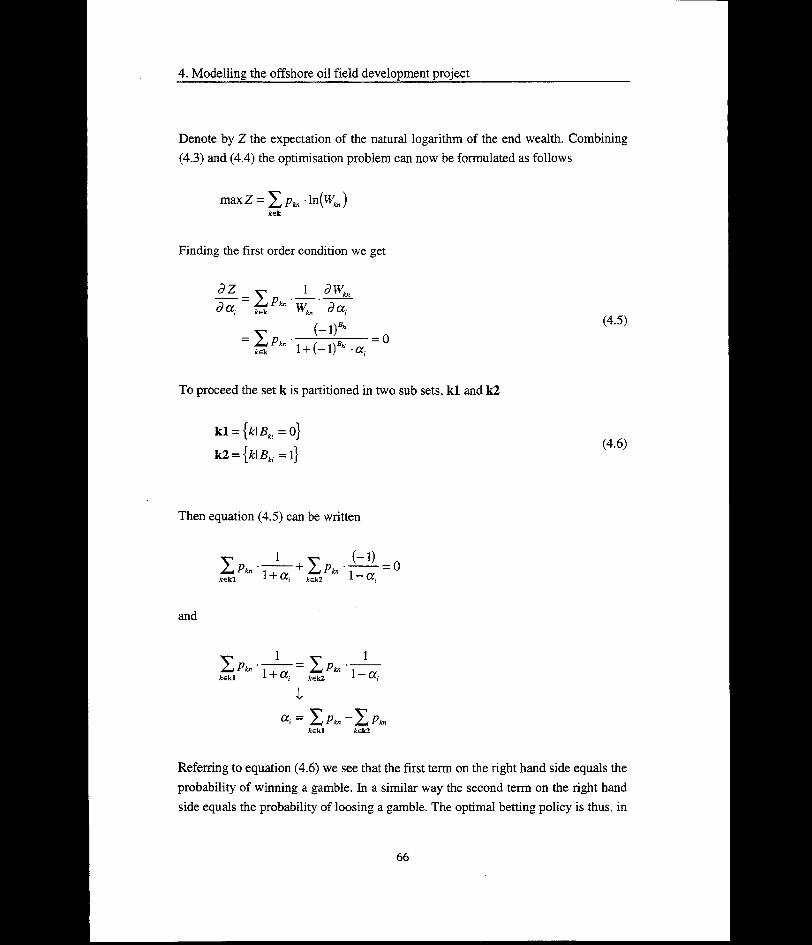
4. Modelling the offshore oil field development project
Denote by Z the expectation of the natural logarithm of the end wealth. Combining (4.3) and (4.4) the optimisation problem can now be formulated as follows
max Z = pkr -ln(w;J&€k
Finding the first order condition we get
= X/,*»ksk
To proceed the set k
L
(-0*i+(-ir
is partitioned in two sub sets, kl and k2
kl = {fcl Bki = o}
k2 = {&l Bu = l}
(4.5)
(4.6)
Then equation (4.5) can be written
!>*■fcskl
11 + CCi
+ 2,p>*iek2
(-1)1 -a.
and
SPtn'1 + CCt = Efkkek2
l1 -a,
a. = X/V, -X^*,fcekl fc€k2
Referring to equation (4.6) we see that the first term on the right hand side equals the probability of winning a gamble. In a similar way the second term on the right hand side equals the probability of loosing a gamble. The optimal betting policy is thus, in
66

4. Modelling the offshore oil field development project
all bets, to bet a proportion of your wealth equal to the difference between p and q. Hence
a* = p-q, i =
Now we solve the same problem by SDP. The fundamental equation of optimality (4.7) is given by Ross (1983). Note that the interpretation of n is different in this problem, n is here the number of remaining gambles the gambler can attend.
Vn (x) = tnax[p • V„„, (x + arx) + q • y„_, (x - anx)] (4.7)
where Vn(x): maximum expected return if the present wealth is x <V share of wealth bet in the n’th last gamble p: probability of winning a gambleq: probability of loosing a gamble
and the boundary condition is given by
V0{x) = ln(x) (4.8)
By (4.7) and (4.8) we get (for n- 1)
y, (x) = max[p -y0(x + tx,x) + q-V0(x- o^x)]
= max[^-ln(l + a1) + ^r-ln(l-a1)] + ln(x)
The first order condition now yields
hence
0) =p-q
67

4. Modelling the offshore oil field development project
Using this result we can rewrite the expression for Vj(x)
Vj(x) = C+ln(x)
where C = In 2+ p ■ ln(p) + q ■ ln(g)
Continuing with n = 2,3,4, — it can easily be shown that
Vn(x) = n-C + ln(x) and a‘ = p- q, Vn
Even though it is impossible to draw a general conclusion of SDP being superior from one example, the solving of the gambling problem shows how simple SDP can be. In this case the effort required to arrive at a conclusion by the standard mathematical technique was considerably higher than the recursive solution technique used by SDP. This computational efficiency is perhaps one of the most important merits of SDP, and is often a motivation for using the method. It thus seems reasonable to use SDP for solving sequential problems like the offshore oil field development project.
4.5.4 Criticism of SDP
However, the choice of a SDP approach does not imply that the method is free of drawbacks. To be fair some of the disadvantages should be referred. Particularly the above mentioned “curse of dimensionality”, and how to derive the discount rate, are non-trivial questions that must be handled in order to achieve a good model. These issues will be addressed in more detail in subsequent chapters.
A more general criticism of operational research (OR) as a decision tool, which inevitably touches upon SDP, is directed towards the inability of OR to grasp the essence of the environment it operates within. One of the most severe attacks are brought forward by Ackoff (1979, 1987) who claims that OR models typically are too static and represent "... mathematically sophisticated but contextually naive techniques”. They thus tend to focus on the solution procedure rather than the solution of the problem. The model proposed as part of this research is designed to evaluate a particular problem and, as such, avoids the accusation of procedure fixation. Nevertheless, if work related to the algorithms is conducted, this should not be viewed as an argument against SDP. Improvement of the procedure does not
68

4. Modelling the offshore oil field development project
contradict the required focus on the solution but rather reduces the time and effort it takes to get there. It might also provide a positive side effect in the form of enhanced understanding of the underlying problem.
Being tailor-made, the proposed model is necessarily static in the sense that a change in environment is likely to require some modification. The addition of new variables will for instance increase the model size and, perhaps, call for adjustments of the data storing capability. It is however hard to see the static properties of the model as a major argument against the SDP approach in particular. One should keep in mind that all models are, at best, adequate representations of the real world. They do not give answers to situations beyond their design. Flexible models are therefore designed with this in mind, usually at the expense of increased development and maintenance costs. The feature of flexibility is also available for SDP models, but must in each case be balanced against the increased cost of obtaining it. The proposed model may thus be viewed as an example where emphasis is put on small development cost.
4.6 A simplified field development description
Having selected SDP as the method for evaluation of flexibility in the field development project, we now turn back to the problem description. The rather detailed phasing given in figure 4.1 indicates the diversity of the tasks involved. In this section the phasing is used as a basis for the simplified problem description.
The desire for a simple problem implies that the number of variables to be included in the model must be small. In addition the time horizon should be manageable. Since both the number of variables and the time is related to the number of phases, the first step towards a simplified model is here to reduce the number of phases.
The selection of variables (and phases) should result in a model that combines the requirements for validity and tractability. This is achieved by capturing the main elements of the field development, with emphasis on those assumed to be of greatest importance to the value of flexibility. The term “assumed” is here used deliberately. It is usually hard to identify all the major elements in advance, and typically the results from model runs provide further insight into the problem. Particularly this is
69

4. Modelling the offshore oil field development project
true for complex systems. In this research the selection is made based on previous research, as well as discussions with Norwegian oil companies.
4.6.1 Phases
The completion of phases in an oil field development project usually reflects milestones. This could for example be the completion of an exploration programme, or the termination of the field. Reaching a milestone implies new information to the decision maker, as any uncertainty related to the completed phase now is revealed. However, equally important is the decisions made available to the decision maker. Finishing one phase means the (possible) start of its successor. In most cases this shift between phases is accompanied by analyses concerning the strategy for the remaining development. For instance will the completion of the exploration programme give information about the reservoir properties, and this information (together with other data) is used to set the production capacity of the concept. Thus phases normally outline the information and decision structure of the project.
Ideally, the number of phases should be sufficient to mirror the decisions and information pattern throughout the project. On the other hand the phases ought to be few enough to keep the evaluation task a manageable one. For an oil field development project these are conflicting goals. Based on the initial phasing (fig. 4.1) an aggregate description of the development stages is therefore proposed. The objective of the rough phasing is to provide a compact basis for the selection of the model variables.
Since the focus is field evaluation, phase one (“Concession”) in the initial phasing falls outside the scope of the thesis. Due to this fact the phase is omitted. Hence, nine of the original phases remain. These are aggregated into four phases according to common traits as follows.
First, the “Seismic survey” and “Exploration drilling” are combined into a general exploration phase. In line with the scope of this study it is assumed that the field is already discovered, and that remaining survey and drilling activity is carried out to gather additional information about the reservoir. The two phases thus have related objectives and deal with the same kind of uncertainty.
70

4, Modelling the offshore oil field development project
The next two phases in the original setting, “Feasibility study” and “Conceptual study”, are in a similar way combined into one conceptual study phase. This overall phase then covers both the preliminary assessments of possible development plans, as well as the final choice of concept. Since the analyses carried out as part of the feasibility study resemble the analyses undertaken when the concept is studied, it seems logical to synthesise these phases into one phase.
The succeeding three original phases are different from the others in two respects. While the oil company in the other phases normally is involved in the activity itself, the engineering, construction and installation is usually handled by contractors. Moreover, due to the contractual terms and conditions between the oil company and the contractors, the uncertainty the oil company is exposed to is of a different nature. Work carried out within these phases is strictly regulated through contracts between the oil company and the sub-contractors of the various job tasks. Even though the contracts do not completely shield the oil company from risk, e.g., due to unforeseen modifications of the platform configuration, they limit the exposure substantially. Thus compared to the other phases the engineering, construction and installation phase is believed to be of minor importance to the overall project risk. As a consequence these three phases are combined into a broad engineering and construction phase. And, in search for a simple model, the phase is treated as deterministic in this study. Note that engineering and construction not necessarily implies the construction of a new production unit, but can also be modifications of existing platforms.
Finally, the two remaining phases, operation and termination, are put into a single production phase. As discussed in chapter 3 an abandonment of the field can be interpreted as a shut down of the operation of infinite length. Termination of the field can thus be conceived of as a last step of the production and treated as a part of this phase.
The framework for the valuation now consists of four phases, of which one (“Engineering and construction”) is assumed not to contain any uncertainty. The new phasing is depicted in figure 4.6.
71
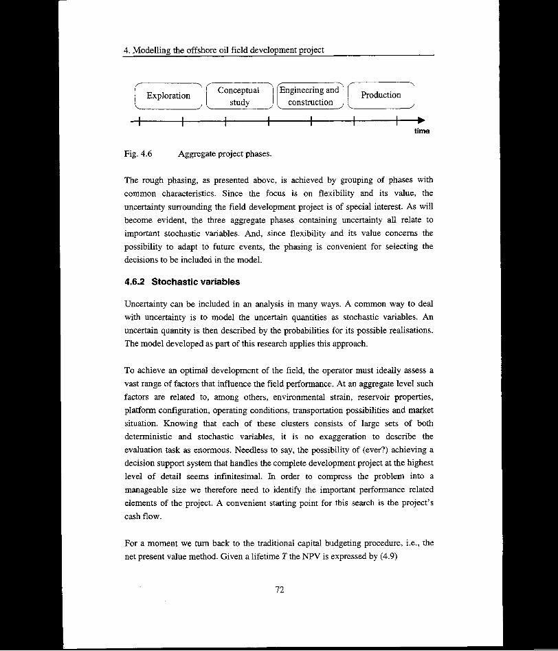
4. Modelling the offshore oil field development project
z >Exploration
L ... j( Conceptual [ study y
Engineering and construction ^
r >|Production
V J
time
Fig. 4.6 Aggregate project phases.
The rough phasing, as presented above, is achieved by grouping of phases with common characteristics. Since the focus is on flexibility and its value, the uncertainty surrounding the field development project is of special interest. As will become evident, the three aggregate phases containing uncertainty all relate to important stochastic variables. And, since flexibility and its value concerns the possibility to adapt to future events, the phasing is convenient for selecting the decisions to be included in the model.
4.6.2 Stochastic variables
Uncertainty can be included in an analysis in many ways. A common way to deal with uncertainty is to model the uncertain quantities as stochastic variables. An uncertain quantity is then described by the probabilities for its possible realisations. The model developed as part of this research applies this approach.
To achieve an optimal development of the field, the operator must ideally assess a vast range of factors that influence the field performance. At an aggregate level such factors are related to, among others, environmental strain, reservoir properties, platform configuration, operating conditions, transportation possibilities and market situation. Knowing that each of these clusters consists of large sets of both deterministic and stochastic variables, it is no exaggeration to describe the evaluation task as enormous. Needless to say, the possibility of (ever?) achieving a decision support system that handles the complete development project at the highest level of detail seems infinitesimal. In order to compress the problem into a manageable size we therefore need to identify the important performance related elements of the project. A convenient starting point for this search is the project’s cash flow.
For a moment we turn back to the traditional capital budgeting procedure, i.e., the net present value method. Given a lifetime T the NPV is expressed by (4.9)
72

4. Modelling the offshore oil field development project
t=T
NPV = Xt=0
CF, f(i+7-y tz
(<?.■)
(l + r)'(4.9)
where CF. is the cash flow in year f, r is the annual rate of return21, p, is the oil
price in year t, q, is the sale of oil in year t and C, (q,) is the total cost (including
investments) in year t. For simplicity it is assumed that the sale equals the production, hence qt can equivalently be seen as the production of oil in year t.
From (4.9) it is evident that three elements are important for the success of the project; the oil price, the production profile, and the cost.
The oil price.
The oil price has received much attention in recent studies, and is commonly regarded as the variable of most significance for the field value. Due to this fact the assessment of the oil price is normally an important part of the field evaluation procedure. From a decision makers point of view the unstability of world market prices is a challenge. As illustrated by figure 4.7 the price may fluctuate substantially even within a short period of time. For long horizons the magnitude of price shifts are typically larger (see chapter 6). When planning the field development strategy this must be handled in an adequate way. A model for decision support under uncertainty should thus capture this property of the oil price. Hence, in the proposed model the oil price is treated as stochastic.
21 The annual rate of return is assumed constant, i.e., r, = r Vr.
73

4. Modelling the offshore oil field development project
14 Oct 96 14 Nov 96
Fig. 4.7 Spot price of oil (Brent Blend) [USD/barrel]. 14 October 1996 - 14 November 1996.
The production profile.
The second element pointed to in the simple cash flow expression is the production (and sale) in each year. At an early stage of the development project the knowledge about the recoverable volume is scarce and experience shows that the understanding of even mature fields are seldom complete (Oljedirektoratet (1995)). Typically this leads to repeatedly adjustments of the estimated reserves. The assessments made for the Ekofisk field over the period 1983 - 1996 (figure 4.8) may serve as an example. In 1983 the field was assumed to contain an economically recoverable oil volume of 271 million Sm3, and about 196 billion Sm3 gas. 13 years later, after continuous adjustments, the estimate was 524 million Sm3 of oil, and 284 billion Sm3 gas. Thus, particularly the estimate of the oil reserves has increased over the years, eventually reaching almost twice its 1983 value.
74

4. Modelling the offshore oil field development project
600
0)0)0)0)0)0)050)050)0)050)0)
■ Oil [million Sm3] UGas [billion Sm3]
Fig. 4.8 Estimates of recoverable volumes for the Ekofisk field.
Uncertainty regarding the reserves is due to both limited knowledge about the reservoir properties as well as uncertainty concerning technological aspects. In other words, the production profile of a reservoir does not only depend on factors such as hydrocarbon source conditions, hydrocarbon preservation conditions, closure conditions, reservoir conditions, porosity conditions, seal and trap conditions, and recovery conditions (cf. Lerche (1992)), but also on technical innovations.
It is not possible to conclude that uncertainty about the reservoir properties is more significant than uncertainty about technical innovations, or vice versa. Nevertheless, for the type of fields considered in this thesis it seems reasonable to put emphasis on the reservoir uncertainty. Since the fields are small, the depletion time is short. Uncertainty regarding new innovations can correspondingly be seen as relatively moderate. It also seems intuitive that the sensitivity of the field value to changes in e.g., reservoir volume is of a larger magnitude than the economic potential from an improvement in technology. Hence, in order to curtail the model size the technological uncertainty is not addresses in this thesis. Without any connection to its importance, it should also be mentioned that assessment of this uncertainty, e.g.,
75

4. Modelling the offshore oil field development project
by density functions for technical innovations, seems extremely hard. Thus limiting the focus to reservoir uncertainty also limits the burden of assessment substantially.
Even if technical uncertainty is discarded the production profile, and thereby the production level and aggregate volume, remains uncertain. Looking back at equation(4.9) it should be evident that this uncertainty is important for the field value. The second stochastic quantity in the model is therefore the production profile.
The cost.
The final element in the cash flow expression is the cost. It has earlier been argued that the uncertainty surrounding the engineering and construction phase is small, and the phase is correspondingly treated as deterministic in this thesis. Any cost uncertainty included in the model should thus be due to exploration, production and abandonment costs.
The exploration activity on the Norwegian continental shelf has been significant over the last decades (see chapter 5.7). This has provided the operators with a broad experience concerning drilling procedures and drilling costs. And in spite of the fact that technical and operational conditions may bring about unexpected challenges, the uncertainty surrounding the drilling cost is usually conceived of as small. In the following the exploration cost is therefore assumed deterministic.
For fields on the Norwegian continental shelf the unit production cost has been stable over the last 6-7 years (Oljedirektoratet (1995)). Even though some increase is expected, the past figures indicate that the production costs have only moderate fluctuations. As a consequence the forecasting of production costs is believed to be “easy”, in the sense that deviations between anticipated and realised cost is small. The uncertainty surrounding the unit production cost is correspondingly of negligible magnitude.
Having ruled out a stochastic exploration and production cost, we finally turn to the abandonment cost. So far only three minor fields on the continental shelf have stopped producing (Mime, Nord0st-Frigg, Odin), and none of the major installations has been removed. For fields developed by fixed platforms the abandonment cost is assumed substantial, and, since empirical support is non-existing, the uncertainty is
76

4. Modelling the offshore oil field development project
high. However, the abandonment cost of moveable platforms do not have similar properties. Being designed for transport, the cost of removing the platforms are small and, if rented, usually made part of the rent. The uncertainty is correspondingly of minor importance compared to price and reservoir uncertainty. All things considered the total cost is therefore treated as a deterministic variable in the model.
The selection of the oil price and the production profile as the uncertain variables in the model is motivated by their importance to the field value. This is in line with the idea of modelling as stated in the introduction to this chapter, and the same choice of stochastic variables can also be found in e.g., Bjprstad et al (1989) and Pindyck (1980). Following the same line of argumentation the construction and production cost is regarded deterministic. Henceforth, the focus will be on modelling of the oil price and the production profile. This topic is addressed in the next chapters.
4.6.3 Flexibility
The discussion of flexibility types in oil field development projects in chapter 3 revealed that all types might be of substantial value to the project. At a general level it is thus hard to determine which flexibility type that should be stressed by the model, and which type that can be handled more leniently. In order not to omit any flexibility types in advance, the model therefore includes all of the four flexibility types identified earlier. The presence of all types should be seen as a sign of the numerous possibilities for decision making that exists throughout this kind of projects.
As for the stochastic variables, the decisions considered in this study are limited to the ones assumed most important for the value of the development project. In line with the discussion made in the previous section, this implies that decisions affecting the production profile are of particular interest. Note that a distinction is made between flexibility types and decisions. Decisions are here seen as means to obtain flexibility, and several decisions can provide the same kind of flexibility types. For example can capacity flexibility result from both the possibility to increase the production capacity of the platform and the possibility to expand the transport capacity.
77

4. Modelling the offshore oil field development project
The flexibility in the project can conveniently be classified as general, i.e., available in all phases, or phase-dependent. General flexibility in the model includes initiation flexibility, termination flexibility and start/stop flexibility.
General flexibility.
The presence of the first type (initiation flexibility) implies that the decision maker can postpone the start of the exploration phase. Since the oil price is assumed stochastic this might be advantageous, as the decision maker will gain more information by waiting. Typically this leads to what is known as a “wait and see” strategy, as compared to the immediate decision of “go”/”not go” obtained from traditional NPV analyses.
Once started, the project contains termination flexibility in all phases. Thus the model allows for an abandonment of the project regardless of the development phase. Apart from the option to stop before the platform is constructed, the termination flexibility gives the operator the choice of when to stop the production. For instance can increased water content of the well stream make it necessary to stop production earlier than planned. Termination flexibility then yields value by avoiding production with negative contribution margin.
Start/stop flexibility is the final of the general flexibility types built into the model. In the first three phases this is an option to halt the development of the project, thereby shifting the whole production profile on the time scale. During the production phase the start/stop flexibility involves an option to temporarily shut down the production from the field. This has a direct effect on the production profile through the associated drop in production. In addition a postponement of the remaining production occurs.
Phase-dependent flexibility.
Phase-dependent flexibility in the model results from decisions made available to the decision maker in some, but not all, of the project phases. Here the included decisions are all related to the production profile, either by affecting the production level or indirectly by providing information about the reservoir. First consider the flexibility in the conceptual study phase and the production phase.
78

4. Modelling the offshore oil field development project
When entering the conceptual study phase the uncertainty about the reservoir is in most cases significant. Particularly the knowledge about the recoverable volume and the production properties of the reservoir is usually imperfect, implying that a concept which allows for subsequent adjustments may be favourable. The term “concept” can be given several interpretations, but typically involves the choice of production unit, e.g., production ship, gravity based platform, FPSO22, as well as the design and production capacity of the unit. In this thesis the assumption of a platform has already been made, and the concept choice is thus limited to design and production capacity. Following the chain of thought presented previously, where emphasis is put on uncertainty surrounding the production level, the concept choice is in this context limited to the choice of production capacity. The production capacity of the platform should here be conceived of as a combined measure of the platform’s production, processing and storing facilities. Hence, the capacity specifies the total well stream that can be handled by the platform.
An important question when so-called flexible concepts are constructed is how much flexibility that should be built into the concept. In other words, to what extent should the concept allow for later adjustments of the production capacity? To facilitate an analysis of this problem, the concept choice in the model involves the decision of installed capacity as well as any free space which provides optional increase of the capacity in the future. Assuming the platform has free space, additional capacity can be installed subsequent to the concept choice.
The second option available to the operator to affect the production profile in the model is by adjustment of the number of production wells. Since the production properties of the reservoir are uncertain, the number of production wells is typically seen as an opportunity to adjust the depletion rate (and, hence, the production profile). This approach is adopted in the model, where the operator can drill production wells during the production period. For instance might a price surge make it profitable to drill additional wells, thereby accelerating the production.
The discounting effect normally gives a strong incentive to start production early, and pre-drilling of production wells is commonly used. To be able to start production when the platform is first located on the field, the model captures the
22 Floating Production, Storage and Offloading.
79

4. Modelling the offshore oil field development project
possibility to pre-drill production wells. This takes place during the engineering and construction phase.
Both the option to increase the platform capacity during the production phase, and the drilling of production wells are examples of capacity flexibility as outlined in the previous chapter.
All decisions introduced so far can be viewed as means to deal with a given uncertainty. They thus provide the decision maker with possibilities to respond to a changing environment, but do not aim at reducing the uncertainty itself. The choice of a flexible platform concept may serve as an example, where the effect of deviations in reservoir properties can be curbed through changes of the platform’s capacity. Instead of dealing with the cause (for the uncertainty) one thus treats the effect. A similar argument is valid also for the other decisions.
Drilling of exploration wells yields flexibility to the exploration phase, and provide another way to deal with uncertainty. The question of how much effort to put into exploration has frequently been raised by oil companies To assess this problem the model reflects the operator’s choice to drill exploration wells. By drilling exploration wells the operator may reduce the uncertainty about the reservoir properties, hence reducing the need for flexible solutions in subsequent phases. Thus, following the terminology used above, the focus is shifted from the effect to the cause. Typically this yields a trade off between the effort to be spent on reducing the uncertainty, and the cost associated with investments in flexible (and more expensive) solutions to deal with the uncertain outcomes.
4.7 Summing up
Based on a discussion of the advantages and disadvantages of three commonly applied methods for project evaluation under uncertainty, the SDP technique has been found suitable. SDP is general in the sense that all kinds of flexibility and uncertainty can be included, and the recursive solution technique provides an efficient solution method. Nevertheless, “the curse of dimensionality” is a challenge that must be conquered.
80

4. Modelling the offshore oil field development project
Two stochastic variables are identified and included in the model, the oil price and the production profile. These are believed to be of major importance to the value of the development project, and will be discussed further in the following chapters. The flexibility in the model is related to each of the four phases of the simplified problem description. All major flexibility types outlined in the previous chapter are included, i.e. initiation flexibility, termination flexibility, start/stop flexibility and capacity flexibility. By including all four types of flexibility the model ought to provide a suitable framework for evaluation of flexibility and its value. Particularly it facilitates a comparison of flexibility types, and is a convenient tool for decision support regarding choice of concept.
Finally it should be noted that handling of uncertainty in the model represents a kind of self insurance. The investment in flexibility and/or cost of reducing the uncertainty corresponds to the insurance premium, while the coverage is the reduced loss (increased income) due to the initial investment. Obviously, this way of dealing with uncertainty is not the only one. A lot of research has been done on the topic of risk management and uncertainty, and the literature on the subject is rich. Possible opportunities for the operator to shield the project from risk span a wide range, and include contracts, risk sharing plans and insurance (to mention some). In particular the possibility of using market instruments (e.g., options, futures and forward contracts) to hedge from market risk has gained much attention in the last decade (see e.g., Hull (1993)). However, to make a thorough discussion of the many alternative methods for uncertainty handling is not within the scope of this thesis. The topic is thus not delved into any further.
81

4. Modelling the offshore oil field development project
82

5. The reservoir
5 THE RESERVOIR
In the simplified project description two stochastic variables were identified; the oil price and the production profile. The production profile of an oil field will depend on numerous factors, and a manageable problem size requires an aggregate representation. The modelling of the reservoir and its properties is thus of primary concern in this context.
This chapter addresses the uncertainty surrounding the reservoir, how it can be modelled, and the effect of dependent well information on the exploration strategy.
5.1 Introduction
Assessment of the reservoir and its properties is among the most difficult tasks in an oil field development project. Based on a given set of input data the reservoir engineer must estimate a large number of parameters, which subsequently are used to describe the production profile of the reservoir. In many cases the input data are encumbered with errors, e.g., due to insufficient measuring methods (cf. Genrich and Sommer (1989)), and the demand for computational power usually limits the size of the model. Hence, the problem is typically of a compound nature, where both insufficient input data and model restrictions are important factors.
The knowledge of the reservoir and the reservoir properties is seldom perfect. Particularly this is true for new fields, but also mature fields conceal information. Experience shows that fields with close to 100 production wells and several years of production still contain uncertainty about the reservoir (Oljedirektoratet (1995)). A general trend of the reserve estimates has been a reduction during the first years of production, mainly due to unforeseen problems. Thereafter the estimates have been adjusted upwards as new information has been obtained and tuning of the depletion strategy has been made. Thus as the project develops the knowledge about the field is improved, and information from production and well drilling provides the operator with a better understanding of the reservoir. However, the initial assessment of the reservoir is necessarily made without this foundation. As a consequence the uncertainty surrounding the reservoir at the time is high. It is at this stage the valuation of flexibility takes place in this thesis.
83

5. The reservoir
According to 0vreberg et al (1992) the input data to reserve evaluations and production forecasts can be divided into three groups (figure 5.1); static data (i.e., data that concerns the hydrocarbon in place estimates), dynamic data (i.e., data that influence the fluid flow), and design data (i.e., data defining the production constraints). Input data within each of these groups are uncertain, and particularly static and dynamic data are scarcely known. In addition there are usually dependencies between the parameters, and a complete assessment assumes that these are identified and quantified. To quantify the uncertainty of the reservoir the operator must therefore estimate a wide range of parameters. And, as the number of required assessments is high, the resources spent on reservoir analyses are substantial.
Static Data e.g.,
- bulk volume- porosity- saturation- net/gross sand
Dynamic Data eg.,
- faults- shales- permeability
Design Data e.g.,
- number of wells- process capacity- drilling schedule- platform design
Fig. 5.1 Input data to evaluation of reserves and production forecasts.
In the oil companies the traditional approach to reservoir estimates and production forecasts has been to describe the field by the data listed in figure 5.1. Based on the data the production profiles are then generated by simulations, where the sensitivity to a selected set of parameters is analysed. The result is a set of possible production profiles which picture the uncertainty.
The level of analysis of this approach is detailed, and the demand on computational power is large. For the purpose of a stochastic reservoir description to be included in the SDP model the level of detail is surely too high. Thus, in order to obtain an applicable formulation, the input data given above should be combined into a limited set of variables. Doing so necessarily implies that a much simpler description is applied, and the challenge is to capture the main features with respect to the evaluation of flexibility. As a consequence our primary concern is not the reservoir as such, but the production profile of the field. This provides an opportunity for an aggregate description.
84

5. The reservoir
In the following sections a review of alternative approaches to modelling the reservoir and reservoir uncertainty is given. To provide a background for the proposed formulation a short description of reservoir models used in previous field development studies under certainty is presented as well. The review is partially based on a previously published report (Bjprkvoll and Lund (1995)) prepared in the research programme PS 2000.
5.2 Reservoir models
Reservoirs are (necessarily) three-dimensional. From a theoretical point of view the reservoir should then be analysed by use of a three-dimensional model, e.g., a simulator. However, in practice lower dimensional models are frequently applied and considered adequate. The reduced level of detail is usually motivated by the gain in assessment burden and required input data. Using lower dimensional models is also favourable due to the associated reduction in computational cost and time.
Lower dimensional models are classified as either two-dimensional or zerodimensional. In the two-dimensional models the reservoir properties vary in the xy- plane, but is homogenous along the z-axis. (The x, y and z axes are orthogonal, and corresponds to the familiar coordinate system from analytical geometry.) These models are commonly obtained by superimposing a grid on the reservoir, and then modelling the interactions between the blocks in the grid. A survey of optimisation models based on a two-dimensional reservoir description is provided by Hallefjord et al (1986).
The simplest reservoir representation is a zero-dimensional model, where the reservoir is homogenous. This model is commonly termed a tank model, and describes a reservoir without spatial variations. Put simply, the parameters of the reservoir are identical all over the reservoir, and location of the wells are of no consequence for the production. As a result it is possible to deplete the reservoir from one single well. The tank model can conveniently be conceived of as a ball filled with oil, where each production well is a straw that can be used to suck up the entire volume.
Reservoir descriptions used in models that aim to find the best development strategy for the field are usually simple, and the tank model is often applied. Examples of
85

5. The reservoir
models based on a zero-dimensional reservoir can e.g., be found in Aronofsky and Williams (1963), Frair and Devine (1975), Beale (1983) and McFarland et al (1984). McFarland et al also give a literature review of related models.
As indicated, the choice of a simple reservoir description can be traced back to computational considerations and the burden of providing detailed input data. Another reason for the frequent use of lower dimensional models is the uncertainty surrounding the reservoir. If the knowledge is scarce, the value of applying a detailed model is questionable. According to Asheim and Hallefjord (1988) it may in fact be disadvantageous, since the detailed information from a complex reservoir model can veil the inherent uncertainty. A simple description can thus be favourable in an early phase of the development project.
5.3 Models of the reservoir under certainty
The frequent use of tank models in contributions dealing with field optimisation makes it reasonable to start with an outline of these models. Thereafter two- dimensional models are presented. Three-dimensional models are not discussed, as these clearly will be too complex for our purpose.
5.3.1 Tank models
The simplest version of a tank model assumes that only one production well is drilled, and that the depletion is driven by the pressure in the reservoir. As a consequence there exists a lower limit for the reservoir pressure, e.g. determined by the pressure of the oil column from the platform to the reservoir. More generally this limit can be considered the abandonment pressure, PTO„, and
where PWJ is the well pressure at time t. The well pressure corresponds in this context to the reservoir pressure. Hence, the pressure at the well head may be different.
As the production goes on, and the reservoir is being depleted, the pressure in the reservoir is reduced. This could for instance be described as in equation (5.1), where the reservoir pressure drops linearly with accumulated production.
86
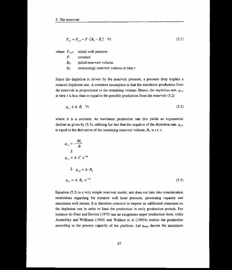
5. The reservoir
(5.1)
where Pw> initial well pressure F: constantR0: initial reservoir volumeR(remaining) reservoir volume at time t
Since the depletion is driven by the reservoir pressure, a pressure drop implies a reduced depletion rate. A common assumption is that the maximum production from the reservoir is proportional to the remaining volume. Hence, the depletion rate, qr,t, at time t is less than or equal to the possible production from the reservoir (5.2)
Qr^A R, Vf (5.2)
where A is a constant. At maximum production rate this yields an exponential decline as given by (5.3), utilising the fact that the negative of the depletion rate, qr,t, is equal to the derivative of the remaining reservoir volume, Rt, w.r.t. t.
^ <?r,0 ~A R0
(5.3)
Equation (5.2) is a very simple reservoir model, and does not take into consideration restrictions regarding for instance well head pressure, processing capacity and maximum well stream. It is therefore common to impose an additional constraint on the depletion rate in order to limit the production in early production periods. For instance do Frair and Devine (1975) use an exogenous upper production limit, while Aronofsky and Williams (1963) and Wallace et al (1985b) restrict the production according to the process capacity of the platform. Let denote the maximum
87

5. The reservoir
production rate due to technical restrictions. Combined with (5.2) this typically yields a production profile as given in figure 5.2.
Fig. 5.2 Production profile for a simple tank model.
The figure illustrates why the extremely simple (compared to reality) tank model has gained acceptance, at least among economists. Even though the tank model does not capture the mass transfer and fluid flow of the reservoir, it provides a profile with resemblance to reality. A structural form of an exponential decline is confirmed by statistics on decline curves for oil and gas reservoir in various petroleum provinces around the world (Nystad (1985)).
5.3.2 Two-dimensional models
Two-dimensional reservoir models are generally more complex than tank models since they include some spatial representation of the reservoir. Normally they are also computationally more demanding.
The obvious effect of going from a tank model to a two-dimensional model is that well location becomes an issue. Since the reservoir has spatial variations, the production from different wells typically differs. Hence, the problem of optimal well
88

5. The reservoir
location arises. In addition comes the modelling of the reservoir, which is more detailed and requires more input.
According to Hallefjord et al (1986), two-dimensional models can be divided into models with an explicit reservoir description and models with a simplified reservoir description. Models in the second class, i.e., models with a simplified description, assume that the reservoir is divided into separate blocks without any interconnections. Compared to the simple tank model the improved reservoir description brought forward by these models are modest. Here the presentation is restricted to models that fall within the first class.
The model proposed by Haugland et al (1988) is used to illustrate an approach commonly found in the literature. In their paper they address the problem of early evaluation of a petroleum field, assuming the platform capacity, the drilling programme and the production level can be decided. The two-dimensional reservoir model is obtained by dividing the reservoir into blocks, where production from a block volume requires that a well is drilled in the block. Maximum production rate from a block is assumed proportional to the block pressure. The interconnection between the blocks is captured by assuming that production from a block not only reduces the pressure in the same block, but also implies a pressure drop in the other blocks. This pressure drop is specified by an influence matrix with fixed elements. Adopting the notation in Haugland et al the maximum production from a block is written as in (5.4)
k=1 j—l(5.4)
where q\: production from block (well) i at time t
J,: productivity index of well i (constant)
p°: initial pressure in (all) blocks
a’~k(i): pressure drop (in pressure units) in period t in block i if welly
produces one unit in period k N: number of production wellsp : minimum well pressure
89

5. The reservoir
The model is an input-output model (Leontief technology). To find the value of the matrix elements a reservoir simulation is carried out, assuming that depletion is taking place from only one well. Hence, in order to specify the complete matrix, the number of simulations required is equal to the number of possible well locations. The model is computationally demanding, and for the complete field evaluation model presented by Haugland et al , i.e., all decisions are made by the model, the authors report numerical difficulties. The problem is also extremely time consuming to solve.
Another way of incorporating a two-dimensional reservoir description in a field optimisation model can be illustrated by the work of Lasdon et al (1986). As for the above presented model the reservoir is divided in blocks, but the interconnections between the blocks are not described by an influence matrix. Instead the equations of the reservoir simulation model is used as constraints in the optimisation problem. The model of Lasdon et al is an operating model, i.e. only decisions concerning the operation are included. Well locations are thus predetermined, and the objective functions used are related to production levels. Compared to the development model of Haugland et al (1988) this implies a significant simplification, even though Lasdon et al claim that their model can be used to decide the number of wells and their locations. No solution times are reported (by Lasdon et al), but the authors indicate that the method is time consuming due to a high number of required reservoir simulations.
5.4 Models of the reservoir under uncertainty
Reservoir models which take into account the inherent uncertainty inevitably become more complex than deterministic models. As a consequence the requirement for a simple reservoir description becomes even stronger, assuming the description is to be incorporated in a unified field evaluation model. Models of the reservoir under uncertainty thus put additional restrictions on the level of detail that can be obtained.
At a general level the production profile can be stated as follows (Lia et al (1995))
<lP{t)=w(r{x),p{t)) (5.5)
90

5. The reservoir
where qp(t): production characteristics at time t if recovery strategy p is followed w(.,.): model for the fluid flow r(x): reservoir characteristics at location x p(t): recovery strategy at time t
The general expression points out two different ways of introducing uncertainty into the production profile. One approach is to derive the production profile from a reservoir model with uncertain parameters, i.e., r(x) is uncertain. The other approach is to omit the modelling of the reservoir, and directly address the description of the uncertain production profile. In the following, examples of both approaches are given.
5.4.1 Production profiles based on reservoir models
Contributions that address the complete development project under certainty are relatively few in numbers. The main reason is probably the computational challenges involved. An introduction of a stochastic reservoir model clearly enhances this problem, and it is therefore no surprise that none seems to have succeeded in combining a stochastic reservoir description with a unified model for field development (cf. Bjprkvoll and Lund (1995)). (A model for exploration decisions presented by Bjprstad et al (1989) combines reservoir uncertainty and a tank model for the reservoir, but the production profile in their model is fixed when the production starts. Thus the reservoir model is deterministic.)
However, several separate studies of reservoir uncertainty can be found, and stochastic modelling of reservoirs with spatial variations has been performed the last ten years (Lia et al (1995). Even though these models are far too complex for our purpose, it is convenient for the later discussion to give an example of the results provided by such models. The GRUS23 project carried out by Lia et al is suitable in this context. Based on a stochastic model for the reservoir characteristics Monte Carlo simulation techniques were used to analyse the uncertainty in the production profile. The oil field Veslefrikk24 was modelled in a case study, and a total of 218 realisations (consuming approximately 1100 CPU hours) were generated. Figure 5.3a and 5.3b show 58 realisations for the accumulated oil production and the production rate, respectively.
23 The Great Reservoir Uncertainty Study.24 The Veslefrikk field was discovered in 1980. It has estimated recoverable reserves of 54.4. million Sm3 oil, 2.7 billion Sm3 gas, and 1.0 million ton NGL.
91

5. The reservoir
The results reveal two interesting properties with respect to a more simple model. First the exponential form of the production decline is easy to spot (figure 5.3b), indicating that the tank type models may give an adequate representation of the production profile. Second there is an almost linear relationship between accumulated oil at the end of the production period and the initial oil in place. Hence, uncertainty in total produced volume can easily be modelled through the initial oil in place.
(a) (b)
Fig. 5.3 Accumulated oil production (a) and oil production rate (b) for the Veslefrikk case study. Source: Lia et a] (1995), figure 13 and 14. 2(f): aggregate production at time t, q(t): production rate at time t.
5.4.2 Modelling the production profile
Studies of development strategies at an early stage is normally carried out at an aggregate level. This, in combination with the scarce knowledge of the reservoir, has brought forward the use of rough estimates for the uncertainty surrounding the production profile. Instead of modelling the uncertainty through the reservoir characteristics, the production profile is assessed directly. Compared to a description based on reservoir models this approach yields a much simpler representation. The uncertain production profile can generally be depicted in two ways.
The most straightforward approach is perhaps to assume that there exists a set of production profiles, where the uncertainty is given by the probability density function for the scenarios. Contributions that handles reservoir uncertainty in this way are e.g., Bjprstad et al (1989), Haugen (1995) and Tjpstheim and
92

5. The reservoir
Stensland (1991). Each scenario can for instance be derived from reservoir models (as in Bjdrstad et al (1989)), or the scenarios can be forecasts based on historical data. Another method is suggested by Bjprkvoll and Lund (1995), who generate the production profiles by Monte Carlo simulation, assuming the reservoir volume, the well rate and the production properties of the reservoir are uncertain.
The assessment of reservoir uncertainty through sets of production profiles provides compact descriptions, but yields no possibility to affect the production by control actions. For the valuation of operating flexibility the approach is therefore of minor interest. Since each production profile is predetermined (and deterministic), no adjustments are available. Hence, the value of flexibility will not be included.
The second approach is to model the production rate as a stochastic process. This approach makes it possible to include control actions, and by selecting the process carefully analytical solutions can be obtained. Typically the Wiener process has been frequently used, due to its advantageous properties (Ekem and Stensland (1993), Olsen and Stensland (1988, 1989), Pindyck (1980), Smith and McCardle (1996)). However, the process should not be selected on these terms, but be chosen in order to mimic the uncertainty in an adequate way.
Stensland and Tjpstheim (1988) studied the production profile for a selection of fields in periods between 1977 and 1987, to see if a model based on the Wiener process was suitable to describe the plateau phase and/or the decline phase. Based on the field data they rejected the Wiener model in both cases, and instead suggested a first order autoregressive process. It should be noted that the data used by Stensland and Tjpstheim give indications of regular fluctuations in production level for some fields, for instance due to maintenance etc. This is not discussed by the authors.
5.5 A simple reservoir model
From the preceding discussion it is obvious that higher dimensional, e.g., two and three-dimensional, reservoir models are too complex for a model that aims to capture the entire field development project. Given the high degree of uncertainty at early stages of the development, it is also doubtful if a detailed reservoir description will provide a better foundation for the relevant decisions than a more coarse description.
93

5. The reservoir
On the other hand, it is also easy to spot the disadvantages of a description that omits the reservoir model, and directly specifies the production profile. For the purpose of flexibility evaluation a set of deterministic production profiles is inadequate, since operating options are excluded.
The description proposed in this thesis is therefore a simple tank model, in which the reservoir uncertainty is captured through uncertain parameters of the model. By using a reservoir model an adequate link to the main reservoir properties is provided. In addition operating flexibility is easy to include. The tank model is of course a coarse approximation of any real reservoir. However, by looking at the results from a three-dimensional model (figure 5.3) it seems as if the tank model is able to reflect the main pattern of the profile (at least for this field). For our purpose this approximation is assumed adequate. Finally it should be noted that the reservoir model relies on input data of a familiar form to the decision maker. For practical purposes this ought to facilitate an implementation of such decision tools in the oil companies.
The tank model used in this study is outlined in Wallace et al (1985b), and is similar to the production model in Bjbrstad et al (1989). The model rests on the following assumptions
(5.6)
and
(5.7)
94

5. The reservoir
where PKj0'- initial well (reservoir) pressure
P W,Z- well (reservoir) pressure at time tPmtn- abandonment pressureRo'. initial reservoir volume
Rt: (remaining) reservoir volume at time t
$r,t’ maximum reservoir depletion rate at time t (productivity of the reservoir at time t)
#W,f' well rate at time tN,: number of producing wells at time t
Equation (5.6) states that the reservoir pressure drops linearly with accumulated production. The expression is similar to the pressure relation presented in section 5.3.1, and is obtained by setting the constant F in equation (5.1) equal to (Pw,o - Pmin)/Ro- Equation (5.7) gives the proportional relationship between the number of producing wells, the well rate, and the relative well pressure above minimum. Since the tank-type model has perfect communication throughout the reservoir, the well rate will be identical for all wells. (If this assumption is not fulfilled, the well rate should be conceived of as an average rate for the producing wells.)
By combining (5.6) and (5.7) the maximum reservoir depletion rate is given as follows
(5.8)
Hence, the right hand side of (5.8) is similar to setting A equal to (TV, • qWtt) / R0 in equation (5.2).
The well rate qWJ as used in this context is not equal to the production capacity of the well. Due to technical constraints it is typically not possible/desirable to produce at the maximum potential, hence the production capacity of a well is given by (cf. Wallace et al (1985b))
95

5. The reservoir
9*.,=y (5.9)
where qw t: production capacity of the well
j. ratio of well production capacity to maximum well potential (y < 1)
The number of producing wells times the production capacity of each well (N, • qWJ) can conveniently be considered the “maximum efficient rate” (MER) for
the reservoir. MER is regarded as the upper limit for the depletion rate of the reservoir, based on technical considerations (Nystad (1985)). A depletion rate above MER implies considerable losses in technically recoverable reserves, while lower rates do not yield a corresponding gain.
In the simple model outlined above, only three reservoir characteristics are modelled; the initial reservoir volume, Rq, the well rate, and the ratio of well production capacity to maximum well potential, y. To describe the uncertainty surrounding the reservoir the two first are assumed stochastic. These two properties are sufficient to introduce uncertainty in the production profile, also in the decline phase. The reservoir volume is specified by its probability distribution, and should be conceived of as the recoverable volume of the field. The well rate is assumed to follow a Markov process, hence it may fluctuate during the production period.
If the production capacity of the platform at time t is denoted qpJ, the maximum production from the field, is given by (5.10)
(5.10)max,:
That is, the maximum production is the minimum of the production capacity of the wells, the production capacity of the platform, and the productivity of the reservoir.
Note that (1 - y) specifies the proportion of total volume produced when the production goes into decline (assuming the platform capacity is not limiting). For instance, if y = 0.75 the accumulated production is 25% of total recoverable volume when the field goes off plateau.
96

5. The reservoir
The production profile for the field can be illustrated by figure 5.4. Here it is assumed that the wells are drilled (and put in production) continuously, i.e., dN—rf- = constant > 0, and the production capacity of the platform is limiting at the at
plateau. The production curve has initially a positive slope as more and more wells are drilled, until the platform capacity becomes the limiting factor. Since the productivity of the reservoir declines as the accumulated production increases, the production is, in the end, curtailed by the maximum reservoir depletion rate, qrJ. Observe that the uncertain reservoir volume and well rate implies that all three production phases, i.e., the escalation, the plateau and the decline phase, are uncertain as indicated by the arrows in the figure. (The plateau level is uncertain because the reservoir productivity may fall below the platform capacity, due to a drop in the well rate.)
If the platform capacity is not limiting, the production profile can still have a plateau level. This happens if the drilling of production wells are completed some time before the productivity of the reservoir becomes the limiting capacity. Then, due to the ratio y, the production capacity of the wells will determine the maximum production from the field and establish a temporary plateau level.
Fig. 5.4 General production profile for reservoir description used in the SDP model.
97
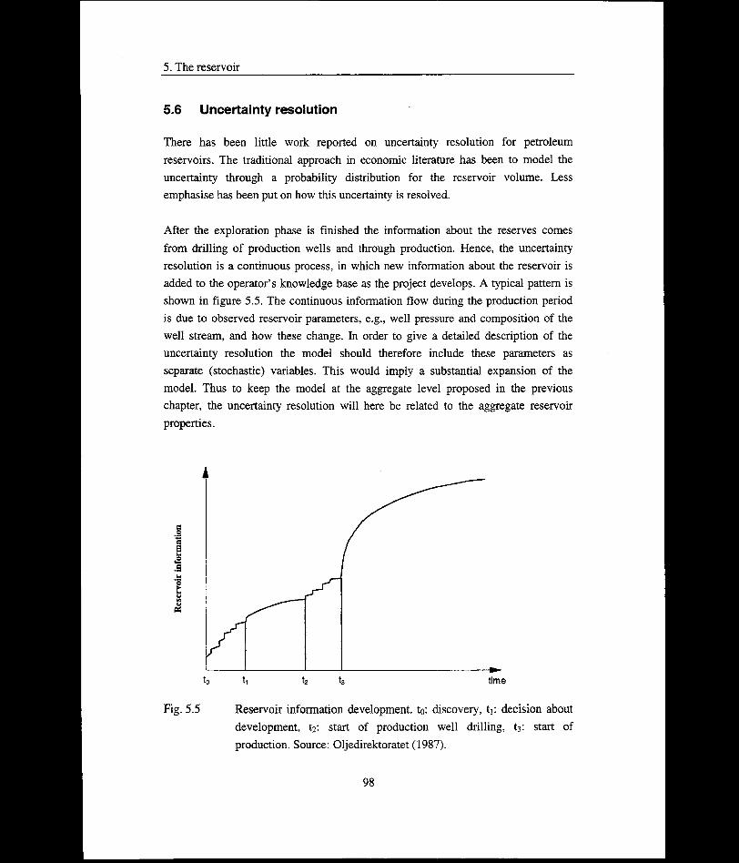
5. The reservoir
5.6 Uncertainty resolution
There has been little work reported on uncertainty resolution for petroleum reservoirs. The traditional approach in economic literature has been to model the uncertainty through a probability distribution for the reservoir volume. Less emphasise has been put on how this uncertainty is resolved.
After the exploration phase is finished the information about the reserves comes from drilling of production wells and through production. Hence, the uncertainty resolution is a continuous process, in which new information about the reservoir is added to the operator’s knowledge base as the project develops. A typical pattern is shown in figure 5.5. The continuous information flow during the production period is due to observed reservoir parameters, e.g., well pressure and composition of the well stream, and how these change. In order to give a detailed description of the uncertainty resolution the model should therefore include these parameters as separate (stochastic) variables. This would imply a substantial expansion of the model. Thus to keep the model at the aggregate level proposed in the previous chapter, the uncertainty resolution will here be related to the aggregate reservoir properties.
Fig. 5.5 Reservoir information development, ty: discovery, ty: decision about development, ty: start of production well drilling, tg: start of production. Source: Oljedirektoratet (1987).
98

5. The reservoir
The foundation for the tank model implies that each reservoir volume has a unique decline rate. Thus in the SDP model the operator learns the true reservoir volume when the production leaves the plateau and starts to decline. Without restrictions on the production capacity of the wells, i.e., y= 1, this will happen immediately after start of production if the platform capacity is not limiting. For a given platform capacity it might then be possible to reveal the true volume by drilling few wells, thereby restricting the productivity of the reservoir. This incentive to curtail the production is avoided by setting y less than 1, since this enforces a plateau level. Thus putting a restriction on the production capacity of the wells does not only limit the production level, but also provides a time lag for the unveiling of the true reservoir volume.
Before the field goes off plateau, the operator is assumed to update the probability distribution of the (remaining) reservoir volume in a Bayesian manner. Since production gives information about the presence of oil, this knowledge is used to revise the operator’s belief about the recoverable reserves. A small example may help to clarify the idea.
Consider for the moment a platform with production capacity of 1 unit per year. So far 10 wells have been put in production and the production capacity of a well for the next production period is Va unit (per year). Then, assuming the production is still at plateau, the maximum production level is 1. Assume further that the operator has a uniform probability distribution for the remaining volume in the segment, with probability 0.2 for a volume of 1, 2, 3, 4 and 5 units, respectively. Each production period is set to two years, and the probability for a depletion of the field within the next production period is then 0.4. The field will go into decline when 1 unit remains (by assumption). At the end of the production period the operator may face two different situations; either the field is depleted during the period, or there is still oil left in the reservoir. The first situation gives the operator complete knowledge, but the second only reveals that the field did not contain 1 or 2 remaining units25. If the latter is the case the operator will adjust his probability distribution based on the new information in a Bayesian manner as follows
25 If the remaining volume was 3 the operator would not have experienced a decline in production during the period.
99

5. The reservoir
— MAX_VOL ’i = d,...,MAX_VOL-x (5.11)
j=x+d
where TT-lx:
d:
x:
posterior probability for a remaining volume of i given a
production of xprior probability for a remaining volume of i
produced volumeconditional probability of producing x and not going into
decline given remaining volume junits left when the field goes into decline
MAX_VOL: maximum volume spanned by the operator’s prior probability distribution
For instance, if 2 units have been produced in the period the posterior probability distribution will be uniform with probability 1/3 of a remaining volume of 1, 2 or 3. (x = 2, MAX_VOL = 5, d = 1, n\ = K2 = ... = K5 = 0.2.)
The second stochastic variable, the well rate, is assumed to follow a Markov process. As for the reservoir volume, the operator is assumed to have an initial probability distribution of the possible realisations, and information about the realised well rate is received through production. The rate can change from one production period to the next, reflecting both variations in physical reservoir conditions that may occur (flow barriers, water-coning, etc.), as well as the operator’s possibility of successfully counteracting such undesirable events. Note that this interpretation does not correspond to an assumption of a homogenous reservoir. The tank model should therefore be conceived of as a framework for development of a simple relationship between important reservoir parameters and production profile, rather than a strict condition. Hence, the reservoir is not completely homogenous.
5.7 Exploration
The possibility to obtain additional information about the reservoir before the development strategy is selected, is generally regarded as an important property of a project. In a study of flexibility and its value, the option to drill exploration wells should therefore be given due consideration.
100

5. The reservoir
The remaining part of this chapter illustrates how dependency between information obtained from two wells affects the optimal amount to be spent on exploration, assuming that the precision of the estimate is improved as more effort is put into the well drilling. It is shown that in situations with a high degree of dependency, an increase in the precision of an additional estimate may distort the operator’s knowledge, and, hence, that the operator could be better off with less exploration effort. A brief discussion of how the cause of correlation influences the results is also made.
5.7.1 Introduction
The uncertainty surrounding the recoverable reserves of an oil field can be traced back to three main areas, namely mapping and description of the reservoir, assessment of the recovery factor and the potential of additional resources not yet identified (Oljedirektoratet (1995)). Among these three areas our main interest is in the first two, i.e., the ones affecting the recoverable volume of the discovered reservoir. We also confine the discussion to the assessment of recoverable volume prior to start of production. In other words, the focus is on estimates based on seismic survey and/or information obtained from exploration wells.
An exploration well provides, through various indicators, information about reservoir rock properties and fluid content. Normally the first wells are dedicated to establish an estimate of the field volume, but subsequent wells may be required to complete and/or refine the assessment. The information from the different wells is, finally, combined into a joint estimate for the reservoir.
The exploration activity on the Norwegian continental shelf has fluctuated over the last years, with a total number of completed wells in the range of 24 - 52 per year (figure 5.6). Consequently the exploration activity’s share of total investment cost in crude petroleum and natural gas production has changed. It is, however, clear that exploration represents a significant part of the Norwegian offshore investments. Good exploration strategies are thus important for the competitive strength.
101
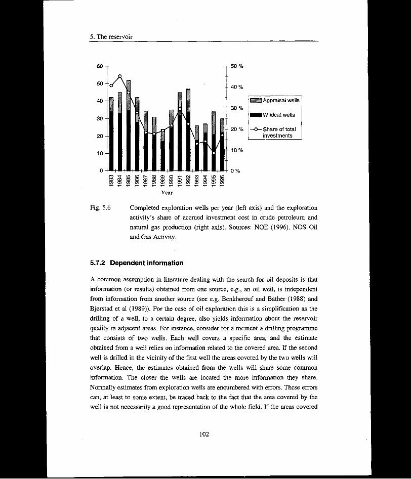
5. The reservoir
60 T t 50 %
CO T LO CO N CO 05 o CM CO *sr LO COCO co CO CO CO CO CO 05 05 05 05 05 05 05a> o> o> o> 05 05 05 05 05 05 05 05 05 05
Year
Fig. 5.6 Completed exploration wells per year (left axis) and the exploration activity’s share of accrued investment cost in crude petroleum and natural gas production (right axis). Sources: NOE (1996), NOS Oil and Gas Activity.
5.7.2 Dependent information
A common assumption in literature dealing with the search for oil deposits is that information (or results) obtained from one source, e.g., an oil well, is independent from information from another source (see e.g. Benkherouf and Bather (1988) and Bjprstad et al (1989)). For the case of oil exploration this is a simplification as the drilling of a well, to a certain degree, also yields information about the reservoir quality in adjacent areas. For instance, consider for a moment a drilling programme that consists of two wells. Each well covers a specific area, and the estimate obtained from a well relies on information related to the covered area. If the second well is drilled in the vicinity of the first well the areas covered by the two wells will overlap. Hence, the estimates obtained from the wells will share some common information. The closer the wells are located the more information they share. Normally estimates from exploration wells are encumbered with errors. These errors can, at least to some extent, be traced back to the fact that the area covered by the well is not necessarily a good representation of the whole field. If the areas covered
102

5. The reservoir
by two wells overlap it is thus reasonable that the errors (of the estimates) are (positively) correlated. A realistic exploration model should take into consideration this interdependency and try to capture the link between information from different wells.
Dependent information has been extensively discussed in relation to combined forecasts and many contributions address this problem (Clemen (1987), Clemen and Winkler (1985, 1993), DeGroot (1974), French (1980, 1981), Lindley (1983) and Winkler (1981).) The general assumption is that each forecast is an estimate made by an expert, and the objective is to combine these estimates into a consensus forecast. A similar situation arises when an operator of an oil field has to combine information from several sources to form a joint estimate. For instance may two or more project teams provide separate assessments of an uncertain variable, e.g., the reservoir volume, from which the operator has to form a combined estimate.
To illustrate the effect of dependent information a simple exploration model is applied. In the model the information is seen as coming from a well. However, the framework is not restricted by such an interpretation and also applies to situations in which the information might be coming from one or more (general) sources. Even though the terminology of wells is used in this thesis, the information may conveniently be thought of as originating from e.g., a seismic survey or a complete separate exploration program involving both exploration wells and seismic surveys.
5.8 An exploration model with dependent information
5.8.1 The problem, assumptions and notation
Consider an operator who is about to develop a field with reservoir volume V,
V = k-ee (5.12)
where & is a constant and Q is a random variable. Through a seismic survey and a completed exploration programme the operator assesses a normal distribution for 6
with expected value and variance <702. Hence, the volume is assumed (by the
operator) to be lognormally distributed. The assessed distribution based on the
103

5. The reservoir
seismic survey and the completed exploration programme can conveniently be seen as the operator’s a priori distribution26.
Before development, another exploration well is about to be drilled at the field, and this well will also give information regarding the reservoir volume. According to the awarded license, the well must be of a minimum depth to fulfil the licensee’s obligations. The variance of the estimate obtained by drilling to the minimum depth is known, but it is possible to increase the exploration effort further to gain more precise information. That is, we assume that the amount spent on drilling affects the accuracy of the obtained information. And the accuracy changes in a predetermined way.
The new well provides information through indicators about reservoir rock properties and fluid content, and this information is used to assess a (separate) probability distribution for 8. To achieve a tractable solution the assessed distribution from the new well is assumed normal. The mean of the distribution, fa,
can be viewed as a point estimate of 6, with
erri = fa-8
being the error of the estimate.
Now, assume that some of the information used by the operator to assess his a priori probability distribution for 6 is also a part of the foundation for the assessment made from the new well. Such common information might for instance occur if the new well is drilled in an area already covered, partially or completely, by previous wells. This situation is in the following referred to as a case with overlapping data, and can be depicted by two experts who base their estimates on samples drawn from a vessel filled with balls. If some balls in one expert’s sample occurs in the second expert’s sample, their data is overlapping.
Due to the existence of common information, the estimation error for this last exploration well is correlated with the estimation error for the distribution based on the seismic survey and the other exploration wells. Let h be the density function of
26 A priori in the sense that it is the operator’s estimate before additional information is obtained.
104
5. The reservoir
(err0, errj), where err0 is the error of the operator’s estimate, h is here assumed bivariate normal, with mean (0,0)' and covariance matrix Z (t- transpose).
The shared information can either be in the form of overlapping data or, more generally, be caused by a common knowledge base for the estimates. (The latter situation is not unusual since estimates to a large extent are formed by professionals with similar training who apply the same models.) If the correlation is caused by overlapping data the correlation coefficient, p, will always be positive (cf. Winkler
(1981)). This is also most likely the case if the correlation is caused by a common knowledge base. The analysis is therefore limited to cases with positive correlation, i.e., pe[0,l). As will be discussed in section 5.10, the cause of correlation is
important with regard to the possible degree of correlation between the estimates. It is, however, of no consequence for the validity of the applied framework.
The operator’s problem is to find the optimal amount to be spent on this last exploration well in order to maximise his expected utility E[u], The decision is final and must be taken before any information from the well is received. Hence, there are no sequential decisions involved.
Let x: additional amount to be spent on drilling, that is, extra effort beyondthe required minimum
p,: mean of the estimated distribution (of 9) based on information from
the well
cr,2: variance of the estimated distribution (of B) based on information
from the well, of = g(x), dg{x) / dx < 0
p: the correlation coefficient (between the estimate errors)27
u: the decision maker’s utility function, u = u(v(6),x)
It is common to state the cost of an exploration well by the cost per feet drilled. More money put into the drilling operation thus means that a larger distance is covered, this be either vertically or horizontally. As the range covered by the well increases, the foundation for the estimate is strengthened. This is likely to improve
the precision of the estimate, and a,2 (the variance of the assessed distribution) is
thus assumed a diminishing function of x. Additional exploration effort then
27 The correlation coefficient is assumed constant.
105

5. The reservoir
increases the accuracy (1 /of). Without any additional exploration effort it is
assumed that the precision of the estimate from the well is lower than the precision of the operator’s estimate. That is, of l.=0 = g(0) > a\.
5.8.2 Variance of the posterior distribution
Since the drilling of exploration wells aims at increasing the precision of the operator’s estimate, an optimal strategy should seek to minimise the variance of the posterior distribution. We here assume that the operator combines the distribution estimate from the new well with his a priori estimate in a Bayesian manner to form his posterior distribution for 6. The posterior distribution, fpost (0), might thus be
viewed as a joint estimate based on two assessments.
Under the assumption of h being location invariant, in the sense that the location of 0 does not alter h, the joint estimate can now be found by applying the results of Winkler (1981). For the general case with k information sources (including the
operator) the joint estimate is a normal distribution with mean fi' and variance <j"
given by (5.13) and (5.14).
H* =e*2Ty/etir1e (5.13)
a2 = 1 / e'ZT'e (5.14)
where e = (1, ..., I)1 and p = (jih •••, tht
As the number of information sources is limited in this context, the general expression can be simplified. With k = 2, the mean and variance of the joint estimate are given as follows
(5.15)(ff02+Oi2-2p<70Oi)
cr(l -p2)g02-g,2
(5.16)
106

5. The reservoir
Note that for zero correlation (p = 0), p* and cr*2 are equivalent to the parameters
of the posterior distribution with the operator’s probability distribution of 6 being a natural conjugate prior (see e.g., Raiffa and Schlaifer (1961)).
Inserting g(%) for cr,2 into (5.16) and taking the derivative w.r.t. x yields
(5.17)(c7c2+s(*)-2pcr0A/gM)2
The right hand side of (5.17) is negative only if the numerator in the bracket is positive. It is thus not guaranteed that additional spending to reduce the variance of the well information gives higher precision of the joint estimate. By solving for
g(x) we find that the derivative of cr*2 w.r.t. x is positive if
(5.18)
From this expression, we observe a somewhat counterintuitive effect which might appear. For situations described by high correlation (see figure 5.7), an increase in the precision of the estimate from the well leads to a higher variance of the joint estimate. The variance increasing effect diminishes as the precision improves, and vanishes when the variance of the joint estimate reaches the variance of the prior estimate. Hence, the latter represents an upper bound on the joint variance
107

5. The reservoir
Exploration effort, x
Fig. 5.7 Variance of joint estimate as a function of exploration effort.
The somewhat strange result is due to two effects that pull in opposite directions.
First is the reduction of the variance O",2, which, in itself, leads to a lower variance of
the joint estimate. However, the decrease in the variance of the well estimate also makes the distribution a more important contributor in the determination of the joint estimate. (A straightforward analogy is to view the joint estimate to be the weighted sum of the two distributions.) Since the variance of the well estimate is larger than the variance of the operator’s assessment (by assumption), the shift has an opposite effect by pulling up the variance of the joint estimate. The net effect on the joint distribution’s variance depends on whether the reducing or the increasing effect is dominant. For a situation with both high correlation and variance of the well estimate, the higher emphasis on the well information is likely to outweigh the effect that can be traced back to the reduced estimate variance. As the precision of the well estimate is increased further, the variance reducing effect catches up on the variance increasing shift, and, finally, makes the slope of the joint variance curve as a function of drilling effort negative. The turning point is given by replacing > with = in (5.18).
A parallel effect to the tug of war between the variance reducing and variance increasing effects can also be seen from equation (5.15). Recognising that the mean of the joint estimate is a weighted sum of two means, we see that the weight given to the mean of the estimated distribution from the well (ji,) changes sign at the same
108
5. The reservoir
time as the derivative of O"*2 w.r.t. x. The confusing effect of increased joint variance
thus has its counterpart in the mean, where the less precise estimate p, obtains a
negative weight for sufficiently high p. As first pointed out by Winkler (1981), this
is due to the fact that a high correlation makes it very likely that the two estimates will be on the same side of 0. Since the less precise estimate is expected to be further away from the true value of 0 than the more precise estimate, the former gets a negative weight in order to obtain a joint estimate that lies on “the right side” of the more precise estimate.
Note that the above effect only occurs when the initial variance of the well estimate is higher than the variance of the operator’s distribution. (Initial refers in this sense to the situation before any additional drilling effort is carried out; thence x = 0.) This
condition follows immediately from (5.18), since min{(c0/p) j = <702. For
situations where the initial variance is lower, the confounding effect of bringing additional information into the system is not present. Given the latter situation, an increase in the precision of the well estimate, by raising x, would always be accompanied by a reduction of the variance of the joint estimate. The reason being that the two effects described above would pull in the same direction.
From figure 5.7 it is obvious that if the correlation between the estimate errors is high, it exists a limit which the additional exploration effort must exceed in order to be effective. Denote this limit x (figure 5.8). Strategies where x is less than or equal to x is then dominated by a strategy that adopts the minimum required drilling (x = 0), and additional exploration effort should only be undertaken if x > x.
109

5. The reservoir
A
Exploration effort,, x
Fig. 5.8 Minimum level x of additional exploration effort that should be applied.
The limit x = x is determined by equation (5.19) with properties specified by (5.20). Since, by assumption, dg{x) / dx < 0, we see that the minimum level for effective exploration effort increases when the operator’s a priori variance is reduced28. In a situation with sequential drilling of wells this means that the required additional exploration effort is higher, ceteris paribus, for wells drillfed late in the exploration programme than for early wells. (Remember that the joint variance after well N is drilled will be the a priori variance when well N+l is about to be drilled. As
o‘ < <7q the result follows immediately.) A strategy based on a constant level of x
will thus inevitably turn ineffective as the number of wells grows. (Note that this rests on the assumption of p being constant.)
g(*) =gp g(o)
(2P-m-°o)(5.19)
28 dx dx dg{x)dal dg(x) dal
110

5. The reservoir
dg(x) 2p-i/g(0)(5.20)
5.8.3 Determining optimal exploration effort
The operator’s objective is to maximise his expected utility, and the optimisation problem can therefore be stated as
Max E{u) = jju(y(e),x) fpos,(G-,Lii,g(x)) f(&-,g(x))dednl (5.21)
where /(jU,;g(x)) is the density function for the mean. The precision of the estimate
is thus known, but the estimate itself, given by the expected value jU,, is uncertain.
To be able to solve the problem, the utility function needs to be established. It seems natural to let the operator’s utility depend upon how well he is able to forecast the reservoir volume. The choice of platform concept and depletion strategy for the field includes various trade offs between such features as production capacity, weight, flexibility, and construction and operating cost (McClelland and Reifel (1986)). Uncertainty about the volume implies that the platform configuration and design should be able to handle a range of reservoir volumes. Hence, the uncertainty requires flexible solutions. The cost of this flexibility might be viewed as a cost of having imperfect knowledge. An improved forecast thus means less need for flexibility and also improves the chance of obtaining an efficient development. A simple, and mathematically favourable, utility function of the following form is proposed
u{V{6),x) = m-e -x, m,v>0 (5.22)
where m and v are scaling constants. The expected utility, E(u), is now readily found
111

5. The reservoir
£'(«) = }{ u(v (9\x)- fpost (0;a, g(x)) • /(rt; g(x))d0
(eV)2(i+2vC-2)= ~X+ e’j2n^e 2a"2 (5.23)
m <j*-J2k
m
Vzvcr^+1
As can be seen, the expected utility is not dependent on the mean of the joint estimate, but merely on the variance. This should not come as a surprise since the utility function measures only deviations from the mean and is invariant to its level.
The variance of the distribution estimated from the well data diminishes with increasing exploration effort. In order to avoid the possibility of zero variance an
exponential relationship between the additional amount x and the variance of is
therefore assumed, hence d2g(x)/cbc2 > 0. Without loss of generality we can
express the initial variance, i.e., before any extra amount is spent on the well, as a
constant a multiplied by the variance O"02 of the operator’s distribution for 9. The
variance of as a function of x then becomes
erf -a-al e sx, a,s> 0 (5.24)
where s is a scaling factor that determines the effect on the variance of spending the additional amount x. (-s equals the relative change in variance from a change in x.)
5.9 A numerical example
Even though the expected utility has a compact expression (equation (5.23)), it is not possible to find the optimal level of (additional) exploration effort x analytically. We therefore have to resort to numerical solutions to illustrate how the operator would
112

5. The reservoir
operate within this framework. For a review of some of the model’s qualities, an artificial set of parameter values is used.
Assume the field about to be developed and the well information structure are characterised by the following
^ o=0 (To = 0.2
a - 2 s = 0.05k = 30 [million Sm3]
We are thus looking at a field of modest size with an expected volume (based on the operator’s assessment) of 33.2 million Sm3 (cf. Hpyland (1976), p. 159). Note that the variance of the well estimate (before any additional exploration effort is carried out) is assumed twice as high as the variance of the operator’s assessment (a = 2). A larger variance of the estimate based on a single well makes in most cases intuitive sense, and would be a typical pattern of fields where the operator collects information sequentially from wells with the same precision. Given that the prior estimate is based on two or more wells, the variance of the estimate from the additional well will be higher (or, in special cases, equal to) the variance of the prior distribution. The larger the information basis for the prior estimate is, the larger the difference in variance tends to be.
The scaling factor s measures the relative change in variance from an additional unit of exploration effort. Hence, a unit change of exploration effort reduces the variance by (approximately) five percent.
The elicitation procedure of the operator’s utility function is not of interest in this context, and will not be discussed. For an introduction to and discussion of decision making procedures and techniques, the reader may consult Morgan and Henrion (1990), Winterfeldt and Edwards (1986) and French (1986). Clemen and Winkler (1993) also offer a brief introduction related to consensus distributions in particular. Here a rather simple approach is applied to derive the value of m. We assume that
113

5. The reservoir
v = 0.5, which corresponds to a moderate relative change in utility for changes in029.
Assume further that the additional exploration effort, x, is given in million USD. To make the two terms in the utility function, (equation (5.22)), comparable, the first term must then represent the money equivalent of the utility from additional exploration. The scaling factor can be found by applying a rough rule of thumb. If the production profile is approximated by a rectangle, a plateau production per year of 10% of the total volume corresponds to a production period of 10 years. Now, to determine the scaling factor, m, assume that the field development is optimised for a field volume equal to the median. This field will then have a production capacity of 3 million Sm3 (== 18.9 million barrels) per year. Due to constraining production capacity, depletion of volumes above the mean leads to a prolonged production period. Compared to an optimal development strategy, this implies a loss in terms of reduced NPV of the sales volume of oil. This loss is used to estimate the value of m. In table 5.1 the change in utility by setting 8 equal to 1 and 2 standard deviations is calculated together with the corresponding values of m. Taking an average and rounding gives an estimated parameter value of 1900.
Tab. 5.1 Estimate of m. Annual rate of return 10%, oil price 17 USD/barrel,average production cost 12 USD/barrel.
8AV
[million Sm3]Discounted loss [million Sm3] Am m
0.447 (1-std.dev.) 16.92 5.94 0.0952 m 1962.2
0.894 (2 std.dev.) 43.38 18.98 0.3297 m 1810.9
Before we go on, it should be emphasised that the above procedure by no means is complete or exact. Its pitfalls are easy to spot, and the majority of cost items and real-life judgements are omitted without any discussion. The purpose and intention has merely been to give some insight into the dimension, and, hopefully, give some feeling for what might be a reasonable range for m.
29 “ „ r *\---------- s= —2vm( Q — Li fla V /
114

5. The reservoir
With the given parameter values, the optimal additional exploration effort is plotted against the correlation coefficient in figure 5.9. For low values of p, an increase in
correlation implies that more additional exploration effort should be undertaken. However, this pattern fades as the correlation coefficient increases, and vanishes when the turning point p' = 0.49 is reached. Thereafter a continued increase of p
reduces the optimal exploration effort. The concave form of the curve is explained by the trade off between the value of information and the cost of acquiring it. When the correlation is low, the last well introduces a high proportion of independent information. As the correlation increases, the reduced value of the well information is compensated for by a higher exploration effort. (The higher effort is a consequence of the positive shift in the marginal benefit of additional exploration effort, which follows from the reduction in well information value.) However, the marginal effect of the additional exploration effort diminishes as the effort is increased, and the exploration cost therefore finally outweighs the corresponding gain. An increase of p (above p') reduces the marginal benefit of additional
exploration effort, and, hence, leads to a lower optimum for x.
50--
2 45 ::
Fig. 5.9 Optimal exploration effort x* for different degrees of dependency between estimation errors.
115

5. The reservoir
It turns out that the optimal exploration effort is relatively insensitive to p over a
wide range for this numerical case. Thus, if the assessment of the correlation coefficient is costly and time consuming, less emphasise should be put on its estimation since an error is likely to be of minor importance. This result will, however, not hold in general but will depend on e.g., the form of the utility function.
So far the choice of the optimal exploration strategy has been made without any restrictions on the possible additional effort. If such a constraint is imposed, the model yields an interesting result in the form of a discontinuous solution with resemblance to a so-called “bang-bang” solution (cf. Dixit and Pindyck (1994), p. 329). The constraint could either be a budget constraint or a physical limitation on the possible well depth and/or horizontal length. In both cases the operator is faced with an upper limit on x which may affect the optimal strategy. Due to the initial increase in the joint estimate’s variance for high correlation coefficients, (see figure 5.7), the operator is, in such situations, better off without a small additional effort. If additional exploration effort should be undertaken, it must at least bring the variance of the joint estimate down sufficiently to cover the increased expenses from the drilling.
The exploration level which makes the operator indifferent to whether he performs the additional drilling or not establishes a threshold value for the exploration effort. Denote the threshold value x\ let the upper limit on x be denoted L, and let the
optimal additional exploration effort in the new setting be x'L. The operator’s
optimal strategy then becomes
L < x1 => x\ = 0
x‘<L => x\ = min{L,x*}
When the respective sources of information are closely related, as measured by correlation, it is therefore not optimal to increase the exploration effort unless this can be done with a sufficient strength. Figure 5.10 illustrates the existence of a threshold value x’. With the given parameters it is clear that additional exploration should not be carried out unless a minimum of approximately 17 million dollars (=%') is spent.
116

5. The reservoir
T 0.201800 -
- 0.181780 -- 0.161760 -- 0.141740 -- 0.12
= 1720 -- 0.10
- 0.081680 - - 0.06
- 0.04
1640 -- - 0.02
10 20 30 40 50 60 70
Expectedutility
Variance of joint estimate
Exploration effort, x
Fig. 5.10 Expected utility and variance of the joint estimate as a function of additional exploration effort x. p = 0.85.
5.10 Correlation caused by overlapping information
Correlation between estimates from different wells can, in general, be traced back to either common information, bias in the analysis of the information, or a combination of both. Even though the applied framework in the previous sections is general in the sense that it is independent of the cause of correlation, the given results are not necessarily obtainable in all situations. In particular we are here interested in correlation as a consequence of overlapping information. Since the utility function remains the same regardless of the cause of correlation we restrict the discussion to the effect on the variance of the joint estimate.
From the derivative of the variance of the joint estimate, <J , w.r.t. x (equation
(5.17)), it is shown (5.18) that a correlation coefficient above cr0-[g(x)] 2 implies
that an increase in drilling effort is accompanied by an increase in the variance of the joint estimate. In the case of correlation due, wholly or partially, to biased estimation procedures, the correlation coefficient can range from zero to one, hence allowing for the results described above. However, if the correlation is caused solely by
117

5. The reservoir
overlapping information, an upper limit is imposed on the correlation coefficient. As described below, this limit is important when it comes to interpretation of the results.
Suppose that both the operator’s estimate and the well estimate of the distribution for B are based on information obtained from (small) blocks of the field. Each block is of known volume, and information from a block corresponds to the outcome of a normal random variable with mean 6 and known variance <r2. The area covered by a well can then be represented by a given number of blocks, and the larger the area is, the more accurate is the estimate. In this setting, the operator’s estimate can conveniently be treated as being based on one single (artificial) well that covers an area corresponding to the precision of the estimate. In what follows, we therefore consider correlation between two wells; one being the substitute for the operator’s estimate (well number 0), the other the new well (well number 1). Overlap between information will now occur if adjacent wells cover the same blocks as illustrated in figure 5.11.
Well 0 Well 1
Fig. 5.11 Field area covered by well 0 and well 1. The shaded squares indicate overlapping areas.
Let A. be the number of blocks covered solely by well i (private information) and
By be the number of blocks that are common to well i and well j (common
information). Hence, the total number of blocks covered by well i is
Nj = A,. + By, i, j- 0,1 i* j. The variance of the estimates, of, and the covariance,
Oy, between the estimate errors are then given by (cf. Port (1994), ch. 13)
118

5. The reservoir
(5.25)(A,-+Sv)'(A;+Sv)
which yield the correlation coefficient p
<7qi (A)+ B01) • (A + 2?01)(5.26)
Va>+3>i Va +VA)+-®oi Va + 3,
An increase of exploration effort, x, now corresponds to an increase of the number of blocks covered by well 1. Assume that new blocks are available in continuously
variable amounts so that the derivative of the joint variance, a , w.r.t. x exists. Thegeneral requirement for the derivative to be negative, given that p is kept constant,
is that p < <70 / <7,. (Remember that <T0 < <r, by assumption herein). From (5.26) it is
easy to show that this is always fulfilled when the correlation is due to overlapping information (appendix B).
It is, however, only in special cases that the correlation will remain constant as new blocks are added to the covered area. Denote the percentage increase in private information to the last well (well 1) by k and the percentage increase in common
information by l. The correlation coefficient p* after new information is added is
then
3,,(1 + /)(5.27)P ~
Note that the effect of a variance reduction is intuitive in that an increase of private information (k > 0) reduces the correlation coefficient, while additional common information (/ > 0) raises the correlation coefficient. For the correlation coefficient to remain constant as new information is added, k must be related to l as given by(5.28). A percentage increase of private information, k, that is higher than the right hand side leads to a reduction of p. Correspondingly, a percentage increase less than
the right hand side results in an increased p.
119

5. The reservoir
l2(A0+B0l) + l(2A0 + Bm)(5.28)
Obviously, a balanced increase of both private and common information as specified by (5.28) yields the same qualitative results as those outlined in the previous section. It is also evident that if information is added in such a way that the correlation coefficient decreases, the variance of the joint estimate will decrease monotonically. We therefore concentrate on the situation where increased exploration effort leads to a higher correlation. To provide a tractable solution, we restrict the analysis to the case where additional information consists only of blocks already covered by the previously drilled well.
The variance of the joint estimate for the case of overlapping information is obtained
by combining (5.25) and (5.26) with the general expression (5.16) for cr*2. By taking
the derivative w.r.t. Bm we get
(5.29)
The derivative is negative only if 2 • B01 • <702 > cr2. By inserting the operator’s
estimate of <r02 and rearranging, the condition becomes Bm> NQ12. The last
expression reveals that if additional exploration effort is carried out when the overlap is less than half of the area covered by the adjacent well, the variance of the joint estimate will increase, (figure 5.12). Note also that the decision whether or not to increase the well precision through adding of overlapping areas is independent of the private information A,. For any given level of A, the operator should thus seek
to maximise (B01 - Ag)2.
120

5. The reservoir
0.15 -
s *
0.14 -
Fig. 5.12 Variance of joint estimate as a function of relative overlap, of = 0.2,
°2 U,=o= 0.4.
We see that the confounding effect obtained for correlation coefficients above a0 / <r, also occurs under certain conditions when the correlation is due to
overlapping information. Even though the correlation coefficient in the latter case always remains less than o0 / Oj, the increased correlation (from adding of common
information when Bm<N0/2) overrides the variance reducing effect from
increased precision of the estimate from the well. In line with the results illustrated in figure 5.10 this implies that additional exploration effort should not be undertaken if Bm < N0 / 2, unless the amount spent is sufficient to overcome the variance
increasing range and improve the expected utility.
5.11 Comments on the exploration model
The analysed exploration model reveals that dependent information can have a confounding effect when the correlation between estimates is high. Increased precision of an estimate obtained from a well can, in such cases, reduce the operator’s knowledge (measured by the variance of his distribution). As a result the operator may be better off without carrying out any additional exploration effort. In
121

5. The reservoir
the event the operator decides to increase the drilling effort when the correlation is high, it should be done with a sufficient strength to override the variance increasing effect on the joint estimate.
While the applied framework is general in the sense that the cause of correlation is irrelevant, the possible degree of correlation is related to whether the dependence is due to biased analysis procedures or shared information. For constant correlation coefficients the confounding effect of increased variance of the joint estimate will only happen if the correlation is caused wholly or partially by biased analysis procedures. However, a similar effect may occur if the correlation originates solely from shared information, given that additional exploration increases the correlation coefficient. In the latter case the qualitative effect is the same as in the case of biased procedures, but is now due to the fact that the growth in correlation more than outweighs the variance reducing effect.
Assessment of the correlation coefficient has not been considered, mainly because the objective has been to illustrate the effect of dependent information. In real-world problems it is, however, not evident how such assessments should be carried out. Neither is it clear what level of precision of the estimated correlation coefficient it is possible to obtain. For the numerical example given in this paper it turns out that the optimal exploration effort is rather insensitive to the level of correlation, implying that a rough assessment might be sufficient. It is, however, not obvious that this result can be carried forward to situations were the figures and/or the operator’s utility function are different from those proposed here. A natural extension of the presented model could thus be to allow for a more general utility function. In particular it seems plausible to make the operator’s utility a function of the expected value for 9, indicating that deviations for large fields are more severe than deviations for small fields.
Another way to carry the model further is to increase the number of new wells. In general the number of wells considered could range from one (as here) to the maximum possible number for the field. However, it seems far-fetched to assume that an operator would not apply a sequential decision rule when the number of wells increases. On the contrary, the information obtained from one well is usually used as input to decisions regarding where and how subsequent wells should be drilled. Bearing in mind the static property of the proposed model, it is thus unrealistic to
122

5. The reservoir
apply this framework to a multi-well setting. To maintain realism the number of new wells (in the problem) should therefore be limited.
5.12 Summing up
A model that aims to evaluate an entire oil field development project faces the challenge of being adequate, and, at the same time, being manageable. This requires a compact description of the reservoir, in order to yield a solvable model. But, the description should also be suitable for evaluation of flexibility. Relevant studies reported in the literature have not managed to combine these two objectives.
The reservoir model proposed here is a tank model, i.e., zero-dimensional in space. This is a very simple description of the reservoir, and clearly represents an approximation to any real field. Even so it establishes a link between (stochastic) reservoir properties and possible production levels. The tank model also describes a production profile with close resemblance to many fields.
Taking into account the operator’s limited knowledge at the time the analysis is made, the simplification of the tank model is considered acceptable. Compared to previous studies the inclusion of a reservoir model represents an expansion, and allows for an evaluation of flexibility in the production phase.
Information about the reservoir can be obtained by drilling exploration wells. If the information from separate wells is correlated, it is important to take this into consideration when an optimal drilling strategy is to be decided. Such correlation can for instance be due to overlapping information, and/or biased procedures. The results given in this chapter show that additional exploration effort to increase the precision of the well estimate, may have a confounding effect on the operator’s knowledge if information is correlated.
The cause of correlation is of importance for its magnitude. However, the confounding effect revealed here can be obtained for both correlation due to overlapping information and biased procedures.
123


6. Oil price forecasting and modelling
6 OIL PRICE FORECASTING AND MODELLING
6.1 Introduction
While the cost items of an oil field development are numerous, the profit relies strongly on one single factor; the price of oil. Since the income is generated through the sale of crude oil, the oil price is crucial for the overall economy of the field. Depending on the net price, i.e., sales price minus production costs, per barrel, the value of the field may vary substantially. An assessment of possible future oil price paths is therefore inevitable when life cycle profit of a field is to be considered.
On the Norwegian continental shelf the trend over the last years has been smaller reservoirs, hence, more fields have become economically marginal. This, together with a declining oil price in real terms, has made new development decisions highly dependent on the forecasts of future prices. However, the information one has come up with by looking in the crystal ball has not always been within an acceptable range of the revealed price, and hardly ever has it been an exact match. In retrospect it is evident where the forecasts failed and/or what assumptions that was wrong, and hopefully past failures improve future performances. But in spite of the knowledge oil companies and analysts accumulate over the years, the challenge of making acceptable forecasts still remains.
The following sections address the nature of crude oil prices, alternative views on how to estimate future price paths, as well as some examples of past forecasting performance. At the end, a suitable approach for the SDP model is suggested. Our main interest is medium and long term forecasts (5-10 years and more), even though some short term forecasts are referred to.
6.2 A historic review
The first Norwegian oil was produced in 1971 at Ekofisk in the North Sea. Since then, and before, the Norwegian, and world, oil markets have been characterised by changes in the crude oil price. These include both long and short term fluctuations.
125

6. Oil price forecasting and modelling
The magnitude of the shifts in price level are illustrated in figure 6.1, which gives the annual average price of Norwegian crude oil for the period 1973 to 1995.
cc 30-
10
i I i.
Year
Nominal1995
Fig. 6.1 Price of Norwegian crude oil (USD/barrel).
Two years after the inception at Ekofisk the Norwegian oil market experienced its first price shock. Due to the Middle East war and the sudden nationalisation of American oil companies operating in the Gulf (Austvik (1986)) the world market oil price increased from USD 5.21 (end of 1973) to USD 10.91 (1974) per barrel. This was followed by a relatively stable market for the next 5 year period from 1973 to 1978, even though there was a small decline in the real price. Then a new shock occured. This time the main cause was the Iranian revolution in the end of 1978 and the subsequent war against Iraq. Due to a sharp drop in production30 and an increased fear of world supply shortages, the crude oil price eventually reached a historic maximum of approximately USD 40 per barrel (nominal) in late 1980, early 198131.
30 The total production of Iran and Iraq in 1979 was 5.7 million barrels per day. In 1981 it had been reduced by 70 percent to 1.7 million barrels per day.31 The spot price of Brent Blend in the last quarter of 1980 was USD 40.93 per barrel, while the corresponding norm price of crude oil from Ekofisk was USD 37.10 per barrel. In the first quarter of 1981 the figures were USD 37.69 and 40.00 per barrel for Brent Blend and Ekofisk, respectively (Statistics Norway, 1991).
126

6. Oil price forecasting and modelling
After the peak in 1980 - 1981 the price started to decline, but with significantly less intensity than the newly experienced rise from 1978. Over a period of four years the annual average reduction in oil price was in the order of 6 percent, bringing the price of Brent Blend down to USD 27.30 per barrel in 1985. The descent came as a result of supply and demand fundamentals, particularly due to increased conservation in combination with an expansion on the supply side. By lowering the oil consumption and, at the same time, raising the production level, the world market made a net gain of 11 million barrels per day (Koutsomitis (1990)). In order to maintain "an acceptable" price level OPEC reduced its production correspondingly. However, the supply and demand pressure outside the control of OPEC continued to evolve. In addition several OPEC members were not able to keep their production at the required level for very long, and in 1986, partly as a result of the signals given by the OPEC's Conference of Ministers in December 1985, the oil price collapsed. In the third quarter of 1985 the spot price of Brent Blend was USD 28.15 per barrel. One year later it was traded for 12.25.
From 1986 till today there have been no shocks of the same magnitude as those that occurred in 1973, 1981 and 1986, even though the prices in some periods have fluctuated considerably. The closest incident in terms of a price surge was the increase from USD 15.90 per barrel in the second quarter of 1990 to a price of 26.05 the next quarter due to the Iraqi invasion of Kuwait32. The escalating price was however quickly calmed, and after a few weeks it had returned to its initial pre-war level. Looking at the figures for the years following the Iraqi invasion, it is striking how steadily the price has declined to its present level. If one were to judge from figure 6.1 one might be tempted to argue that the price pattern shows a clear mean reverting tendency, and that the fluctuations are mere deviations from the long run price level. Whether this is an adequate view or not is addressed below.
So far the reasoning has pointed towards political events as the major source of price shocks and fluctuations. It should however be mentioned that alternative views exist, where the political events are seen as the results of underlying economic imbalances (see e.g., Liao and Lin (1995)). The latter approach thus sees the political event as the effect and the imbalance as the cause, while the former views the political event as the cause leading to price movements (and imbalances). In the end this is just a discussion of cause and effect.
32 The spot price per barrel briefly touched the 40 dollar mark (Petroleum Economist, 1991). Due to its short existence the jump of the average price was less dramatic.
127

6. Oil price forecasting and modelling
The purpose of this brief historical review has been to provide a background for the following discussion regarding oil price forecasting. It has had no intention of being complete, and the explanation of price movements has only been given as a broad outline of the underlying causes. For a more thorough discussion and review of the oil price history, see e.g., Austvik (1986), Koutsomitis (1990), Griffin and Teece (1982) and the references therein.
6.3 Alternative views
The world oil market is a market with numerous unpredictable actors. Both private as well as national interests are at stake, and oil companies, consumers, and national governments are likely to pursue their goals in the best way. The objectives of the actors may be common, but the situation is generally seen as a tug of war over scarce resources.
In order to arrive at a comprehensive model of the oil market, all elements should be taken into account. That is, strategic choices, bargaining processes, supply and demand characteristics, governmental regulations and so on, should all be explanatory variables in the model. Obviously this is not a viable approach. Such a model would inevitably get out of hand. It could also be argued that it would violate the core issue of modelling, namely to capture the essential variables and omit the less important ones.
The apparent need for a reduced representation has been treated in the literature in various ways, each reflecting the purpose of the analysis. On an aggregate level these can be grouped into three categories, here named scenario/qualitative models, economic models, and stochastic processes. It should however be noted that the distinction between the two first is not sharp. The last group, stochastic processes, differs in theoretical foundation. For reasons to become obvious in later sections the stochastic processes are emphasised.
128
6. Oil price forecasting and modelling
6.4 Scenario/qualitative models
The scenario/qualitative models emphasise the political and strategic interactions between the market participants, normally at an aggregate level, to arrive at a forecast for the coming energy situation. They thus give a broad outline of the expected future, while details and microeconomic concepts are of minor interest (see e.g., Austvik (1986)).
Even though the elements taken into account differ among the analyses, some key factors seem to form part of most approaches. First of all the major producers in the world oil market are included, either divided into OPEC and non-OPEC countries (e.g., Austvik (1992)), or by a more detailed partition (e.g., Koutsomitis ((1990)). Second the demand side has to be characterised, usually by an average energy consumption in percent of the GDP. To arrive at an estimate of tomorrow's oil prices one then prognosticates the development concerning:
- Exploration effort / New Resources- New production technology / production capacity- Conservation of demand- New technology / substitutes (yields reduced demand for oil)- Governmental regulations- GDP / World Economy- Influence / power of coalitions and organisations (e.g., OPEC, DBA)
Usually a few scenarios, say two or three, are developed on basis of the given assumptions. This would typically be a worst case (pessimistic) scenario, a most likely ("neutral") scenario, and a best case (optimistic) scenario. The probability of the different outcomes are rarely quantified.
The advantage of the above approach is that the aggregate level and the coarse description allow for a long forecast horizon, often 5-10 years or more. This makes the technique suitable for strategic planning. The horizon should also be reasonable for large scale projects like offshore oil field developments. However, the limited (or non-existing) quantification of the uncertainty hampers the usefulness severely. One might thus say that the advantage from a strategic point of view becomes the disadvantage from an operational point of view. Decision makers at project level are
129

6. Oil price forecasting and modelling
seldom comfortable by making decisions based on "vague descriptions" of the future.
6.5 Economic models
“Economic models" as the term is used here offer a more quantitative approach to oil price forecasting. In contrast to the scenario/qualitative models the behaviour of the market participants are modelled specifically, normally under the assumption that participants seek wealth maximisation33. The major gain from this approach is that the uncertainty, if present in the model, is quantified. (The quantified uncertainty is not a solution, but an input to the model.) The major loss is the increased demand for information and computer resources to solve the model.
Even though economic models have a more quantitative nature, the main elements are the same as those found in scenario/qualitative models. This means that a supply side consisting of OPEC and non-OPEC countries (alternatively with a more detailed partitioning) is kept, together with a single demand side. The focus on the supply side is a typical pattern found in the literature. This is somewhat surprising, as, according to Koutsomitis (1990), "the demand side is the one with the greater degree of uncertainty". It thus seems like emphasis has been put on modelling of the side believed to be most easy to grasp, while the challenges associated with obtaining an adequate description of the demand side have been neglected. This is a weakness of the considered models.
Due to the computational problems that go along with models of this kind the number of variables is in most cases smaller than the number possible to include in a more qualitative assessment. Two recent contributions are here given as examples, one with uncertainty, the other without. Both demonstrate computational obstacles. For an overview of older oil market models, see e.g., Hammoudeh (1979) and the introduction of Sal ant (1982)34. Some discussion is also found in Marshalla and Nesbitt (1986).
33 An alternative description could for instance be a target revenue objective.34 Salant (1982) propose a Nash-Coumot model for the oil market where the agents use open-loop strategies. Uncertainty enters the model through a constant probability of an oil plant being nationalised, and through several possible outcomes to be revealed in the future (at a known date).
130

6. Oil price forecasting and modelling
The model developed by Lensberg and Rasmussen (1991) is an example of an economic model used to forecast the oil price under uncertainty. The main feature of the model is, as the authors state, "that the uncertainty about OPEC's price strategy is assumed to be generated not by irrational behaviour on the part of OPEC, but by uncertainty about OPEC's size and time preference". It is a long run intertemporal model which encompasses four market participants, namely three groups of oil producing countries (OPEC, non-OPEC, and OPCA35) and one demand side. By treating the net export of the OPCA countries as a part of the demand side, the model is reduced to three groups. The model formulation is correspondingly split into three separate modules, one for each group of agents. An optimal price strategy for OPEC (as a whole) and an investment strategy for the non-core countries (usually the OPEC members except for Saudi Arabia, Kuwait, UAE and Quatar) is then determined by solving a stochastic dynamic programming model. Given the OPEC history since 1974, the model reproduces the price development from 1974 to 1989 fairly well in a model experiment.
The second contribution is given by Young (1994), who describes a framework which combines the monopoly aspect of OPEC with the non-optimizing, flexible behaviour of OPEC's individual members. As for the model of Lensberg and Rasmussen the key variables are the optimal price path and the required investment level. The forecast for the optimal OPEC price is found by a two step procedure. First the optimal path is found for any given member by solving a constrained optimisation model. Then these paths are seen as input to a bargaining process, where the agreed OPEC price is given by a weighted average. Young's framework is however deterministic, but in spite of this significant simplification (compared to the Lensberg - Rasmussen model) Young does not manage to solve the model.
Economic models of the kind exemplified above thus offers a quantitative approach to oil price forecasting, but are computationally demanding. This is the major drawback of these models, and is likely the main reason why, to this author’s knowledge, few applications of similar models exist.
Before we turn to the stochastic processes, the work of Hotelling should be mentioned. In the seminal paper in the early 1930s he proposed a framework for
35 The producing countries outside OPEC are either classified as non-OPEC or OPCA. Non-OPEC countries have market economies, while the rest belong to OPCA (Oil Producers in the Communist Area).
131

6. Oil price forecasting and modelling
determining optimal depletion of an exhaustible resource (Hotelling (1931)). Under the assumption of known oil reserves, costs, and a perfect market, he showed by calculus of variation that the maximum present value to the oil producers is obtained when the net oil prices increase at a rate equal to the discount rate. This rule was later expressed as the "Hotelling Valuation Principle", stating that the value, V, of one in-ground unit of the resource had to equal the net price, P:
V(O) = P(t) ■ e‘! = P(0) ■ eg! ■ e“ = P(0)
where t: timeg: growth rate of net oil price (= i (Hotelling's rule))i: discount rate
Hotelling's simple, but elegant, formula has frequently been used as a basis to forecast oil prices. (The forecasts are made by assessing the future development of variables that influence the oil market, e.g., the cost of incremental oil supply. These assessments are then combined with Hotelling’s rule to forecast the oil price.) Its efficiency, especially for long term prognosis, can however be questioned (see the discussion in section 6.7). An example of the use of Hotelling's rule is found in Oliveira and Lodi (1994).
6.6 Stochastic processes
Both the scenario/qualitative models and economic models have the common feature that they rest on some fundamental theories of the behaviour of the actors of the world oil market, and that the oil price is determined by supply and demand interactions. For a wealth maximisation approach this would typically span from an assumption of competitive markets on the one side to monopoly on the other side. In between various models of the market exist (cf. Gravelle and Reese (1988)). While these qualities may be more distinctly declared in the economic models, it is also the notion of a market equilibrium which forms the basis for forecasts in the scenario/qualitative assessments.
Stochastic processes, however, do not have the same connection with the market. That is not to say that they are unable to mirror the fluctuations of the oil price. On the contrary, this is, in our context, the purpose of applying a stochastic process. But,
132

6. Oil price forecasting and modelling
instead of modelling the market mechanisms (as discussed in the previous sections), the focus is on the random price movement itself. The justification for such an approach is mainly related to the fact that to market participants without any significant influence on the market, the oil price looks erratic. A quick glance at the price path in figure 6.1 explains why this view has gained acceptance among (at least) economists.
One of the reasons for choosing a stochastic process instead of a more comprehensive model is to accomplish a more convenient representation regarding applicability and solution time. To obtain this, it is desirable that the process satisfies the Markov property. The Markov property ensures that only the present value of a variable is relevant for predicting the future. The probability of a rise in, say, the oil price tomorrow, is thus only dependent on the price today. Not on yesterdays price, the price before yesterday, and so on. In the literature concerning oil price modelling the Markov property is fulfilled for the two dominant processes, namely the Brownian motion and the Omstein-Uhlenbeck process.
6.6.1 Brownian motion
The Brownian motion36 was first observed and described for the motion of small particles suspended in a liquid as these were affected by successive and random impacts from neighbouring particles. Recently the process has gained popularity also in other areas, and has frequently been used to model the prices of financial assets and raw commodities, including oil37. Especially literature within the area of option pricing theory has heavily applied the assumption of the stochastic process being a Brownian motion. (This has been the case also when the stochasticity of e.g., project values, costs and physical volumes have been modelled. In many cases these assumptions are highly questionable, and are typically made to obtain tractable solutions.)
36 Named after the Scottish botanist Robert Brown (1773 - 1858).37 See for instance the pathbraking paper by Black and Sholes (1973), Geske (1979), or Hull (1993) for examples of financial assets described by a Brownian motion. Bjerksund and Ekem (1990), Brennan and Schwartz (1985), and Dixit and Pindyck (1994) describes raw commodities by a Brownian motion.
133
6. Oil price forecasting and modelling
The Brownian motion has three important properties:
- It is a Markov process- Increments over a finite interval of time are normally distributed- The increments are independent
Based on the basic Brownian motion - also known as a Wiener process (equation (6.1)), the oil price is usually modelled as a Geometric Brownian motion with drift (equation (6.2)).
dz = s4dt (6.1)
dP_P
adt -r adz (6.2)
where P : oil pricee: normally distributed random variable ~N(0,1)a: drift ratet: timea: variance parameterdz: increment of a Wiener process. E[dz] = 0, Var[<fe] = dt
From the above equation it is evident that an oil price that follows a geometric Brownian motion tends to move away from its initial value (assuming the drift rate is not zero), either reaching for a lower bound of 0, or moving towards infinity. Since the increments of dP/P are normally distributed, the absolute changes in the price, dP, will be lognormally distributed. The expected value of P at time t is given by
E{P(r)} = />( 0)-e" (6.3)
where E denotes an expectation, and P(0) is the price today. Figure 6.2 illustrates a possible price path for an oil price described by a geometric Brownian motion.
134

6. Oil price forecasting and modelling
=e 30 -
10 -
Fig. 6.2 Sample path (solid line) of a geometric Brownian motion, a = 0.02,
a = 0.2. The dotted line is the expected value of the price.
6.6.2 Mean reverting process
The tendency for the Brownian motion to move far away from its initial position has been questioned for commodity prices. A common view is that the price for such goods should be related to the cost of producing them, and thus, in the long run, ought to approach the marginal production cost. In the framework of the scenario/qualitative models the deviations from the mean would then correspond to impacts from wars, changes in OPEC's position, supply/demand interactions, etc.. These deviations would only be temporary.
The above described property is obtained through the use of mean reverting processes, where the mean equals the marginal production cost. The simplest mean- reverting process is the Omstein-Uhlenbeck process given in equation (6.4)
135

6. Oil price forecasting and modelling
dP = —t](p - P)dt + adz (6.4)
where P: oil pricetj: speed of reversion
P: level the price tends to revert to (the mean)t: timea. variance parameterdr. increment of a Wiener process
The Markov property and the property of normally distributed increments are also found for the mean reverting process. But, due to its autoregressive quality, increments are no longer independent. That is, the further away the process has reached from its mean, the stronger is the tendency for a movement towards the mean. The effect can be illustrated by concidering a dog who is tied to a pole with a rubber band. Here the pole functions as the mean, while the dog’s distance from the pole corresponds to deviations from the mean. The further the dog has walked away from the the pole, the stronger is the pull towards it.
The mean reverting tendency of the Omstein-Uhlenbeck process is clearly seen from
the expected value of future prices (equation (6.5)). As r —> > P. We
also note that the smaller t] is, the more the price will tend to drift away from its
mean. Setting 77 = 0 yields a simple Brownian motion.
(6.5)
Figure 6.3 shows possible price paths for the oil price, depending on the level of reversion. The price paths are based on the same simulation for the Wiener process as the sample path for the geometric Brownian motion given in figure 6.2. For comparison the geometric Brownian motion is therefore superimposed in figure 6.3. As expected the Omstein-Uhlenbeck process yields a tighter price range than the geometric Brownian motion, in particular for large values of 77.
136

6. Oil price forecasting and modelling
Fig. 6.3 Sample path of an Omstein-Uhlenbeck process for different reversion
levels. <7=3.4, P = 17 (USD/barrel). GB denotes the geometric Brownian motion.
6.6.3 Empirical and theoretical guidance
Several empirical studies have been performed to see whether the oil price is best modelled as a Brownian motion or a mean reverting process. The results are mixed, and give no firm conclusion or preference for one or the other. Dixit and Pindyck (1994) tested if the arithmetic Omstein-Uhlenbeck process
dP(t) = -rj[p{t) - P)dt + adz (66)
was suitable for modelling the spot price of oil. From an analysis of the price of crude oil for the period 1870 to 1990 (figure 6.4), they found that the price has a mean-reversion pattern if the whole period of 120 years is considered. Nevertheless, the speed of reversion is slow. For shorter intervals of 30-40 years it is not possible to reject the random walk (e.g., geometric Brownian motion) hypothesis.
137

6. Oil price forecasting and modelling
H—I—I—I—1
1870 1910 1970
Fig. 6.4 Price of crude oil in 1967 US dollars per barrel. Source: Dixit and Pindyck (1994), p. 78.
In an earlier paper Pindyck (1988) tested the reverting price process
d\nP{t) = r}\n{P! P{t))dt + dz (67)
where Pity.
n-~P: dz:
oil price at time t speed of reversion
level the price tends to revert to (the mean) increment of a Wiener process
but was not able to draw any conclusion whether the oil price encompasses a reverting quality or follows a random walk.
The findings of both Dixit and Pindyck (1994) and Pindyck (1988) are in line with that of Gibson and Schwartz (1991), who are unable to detect a mean reverting pattern in the “steady-state” spot price of crude oil over a period of two years38.
38 26 Nov. 1986 - 18 Nov. 1988.
138

6. Oil price forecasting and modelling
However, the time horizon is seen as too short to draw any definitive conclusions. (The period only captured a downward trend in the oil price, not an entire cycle.)
A contradictory conclusion is reported by Jamshidian (1990), who infers the dynamics of the spot price from the futures term structure. This yields the following stochastic process
dP(t) / P(t) = \b{t) - a{t) In P(t)]dt + o{t)-\dz + X{t)dt\ (6.8)
where P(t): oil price at time ta(t): mean-reversion parameter dz~. ■ increment of a Wiener process X(t): market price of risk
b(t) and c(t) are deterministic functions
Based on a study of monthly (and weekly) spot oil prices for a period of 6.5 years39
Jamshidian rejected the random walk hypothesis, and found evidence of mean reversion. A similar result, although based on expectations, is given in Bessembinder et. al. (1995). They use the term structure of futures prices to investigate whether investors expect mean reversion in spot asset prices. For crude oil, the estimated mean reversion is large40. The study uses daily settlement prices for the futures market for the period January 1982 to December 1991.
Since it is impossible to make a clear choice of stochastic process based on empirical studies, one may resort to theoretical considerations. As indicated above the argument for a mean reverting process is linked to supply and demand characteristics. In a situation with low oil prices the (relatively) high demand will not be matched by the producers, who obtain a low return on their investments. Eventually the prices will rise to close the gap between supply and demand. A high oil price will correspondingly induce a supply surplus, both due to reduced demand as well as increased oil production. This surplus can not exist for a long period of time, and the price will gradually decline. The criticism raised against the possibility of “infinite” prices of the geometric Brownian motion is therefore not relevant for
39 28 Jan. 1983-27 Jul. 1989.40 As an example they report that point estimates show that 44 percent of a spot oil price shock is anticipated to be reversed over the following eight months.
139

6. Oil price forecasting and modelling
the mean reverting process. Hence, based on economic theory the mean reverting process is somewhat more acceptable than the geometric Brownian motion.
The Brownian motion is not founded on any economic theory, even though it may be argued that the exponential growth of the expected future oil price for a geometric Brownian motion with positive drift is compatible with Hotelling's rule. As indicated earlier the frequent occurrence of the Brownian motion in economic literature is however more likely a consequence of its favourable mathematical properties. Evaluation of projects where the underlying stochastic variable follows a random walk are normally easier than projects with variables modelled by use of mean reverting processes. While the former in most cases yields tractable, analytical solutions, the latter must be solved numerically. Lund (1993) in fact argues strongly against the use of a geometric Brownian motion to model the oil price. Under a set of reasonable assumptions he shows that the geometric Brownian motion can not be an equilibrium process due to asymmetric supply response in the market to price changes41. Lund does not however completely rule out the possibility that there may exist other sets of assumptions under which the geometric Brownian motion is an equilibrium process.
6.7 Forecasting in retrospect
It should come as no surprise that a review of past forecasts of the oil price reveals many failures. The pitfalls are numerous, and even though many different interpretations of the mechanisms that govern the price has been put forward, none has managed to provide reasonable predictions of the fu ture (c.f. Oliveira and Lodi (1994)). The bad record confirms the unpredictability of a market made up of many actors with divergent objectives and strategies to pursue them. These challenges of price forecasting are of course not only related to oil, but is common for many traded commodities. However, this fact is a poor consolation when the oil price is the one to be predicted.
Empirical studies show that many recent forecasts of the oil price comply with the valuation principle of Hotelling. Hotelling's rule is founded on the assumption of oil being a non-renewable resource, yielding a rise in the long run competitive price due
41 Under the given assumptions the aggregate demand is a Markov process, but the aggregate supply is not.
140

6. Oil price forecasting and modelling
to growing scarcity. The pattern of growing prices is apparent from figure 6.5. As can be seen from the figure, the levels of the forecasts are adjusted according to the actual price at the forecast time, but the positive slope is maintained.
100 T
§ 50 --
a 40 -
20 --
Year
--------- Actual price* December '81
- ■ * - - July '83- - X - - January '85- - ♦ - - January '86
Fig. 6.5 Crude oil prices (1990 $/barrel). Actual and successive TEW (International Economics Washington) polls. Source: Adelman(1993), p. 3.
The positive slope of the projected price path is also evident from table 6.1, which is based on projections from 17 oil companies and financial institutions. Another interesting feature of the forecasts is that the range described by the high and low estimates envelope the actual price path apart from the shock in 1990. It thus seems like modest fluctuations are captured by the analysts, while profound incidents are harder to grasp. This is rather intuitive, but illustrates the challenge of forecasting the world oil price.
141

6. Oil price forecasting and modelling
Tab. 6.1 Forecasts (of 1988) and actual annual average spot price for WestTexas Intermediate for the years 1989 - 1993 (USD/barrel). Source: Oil & Gas Journal, May 22, 1989, Statistics Norway (1995).
1989 1990 1991 1992 1993High forecast 21.22 22.07 22.96 23.87 25.00Average 16.60 17.70 19.06 20.36 21.91Low forecast 14.00 14.00 14.43 15.15 15.91
Actual price 19.65 24.85 21.00 20.55 18.45
The efficiency of forecasts has recently been assessed by MacDonald and Marsh (1993). For the rather short forecast horizon of three months they concluded that in a number of instances forecasters could outperform the random walk. (The sample was monthly three-month forecasts for the period October 1988 to March 1991, yielding a sample size of 18 observations.) However, price shocks due to the Iraqi invasion of Kuwait in 1990 was not captured by any forecast. They also found that the forecasts in most cases were biased, indicating that the financial market was informationally inefficient42. In line with this, forecasters world wide were found to have heterogeneous expectations.
In spite of the low hit rate of previous projections, the tendency for forecasters to anticipate a growth in the oil price is not a past habit. A comparison of eight projections for the period of year 2000 - 2010 (table 6.2) shows that the beliefs in an increased oil price is still present. Whether they are more successful this time than in history remains to see.
Tab. 6.2 World oil price projections for 2000 - 2010 (1993 $/barrel)43. Source:Energy Information Administration, 1995.
Year IE095 IEA PEL DRI WEFA GRI NRC CEC2000 19.31 23.00 14.99 19.98 18.75 18.58 20.00 21.062005 21.50 28.00 14.15 24.67 20.36 — 22.00 23.21
2010 24.12 28.00 14.97 28.07 21.36 20.54 22.00 25.56
42 A financial market is informationally efficient if all available information is discounted into the current asset price.43IE095: International Energy Outlook 1995, IEA: International Energy Agency, PEL: Petroleum Economics Ltd., DRI: DRI/McGraw-Hill, WEFA: The WEFA Group, GRI: Gas Research Institute, NRC: Natural Resources Canada, CEC: California Energy Commission.
142

6. Oil price forecasting and modelling
From the discussion in this and previous sections it is reasonable to ask whether the oil price can be forecasted with a sufficient degree of accuracy or not. In other words, is it possible to foresee the various incidents that may have an impact on the oil price for the next 5-10 years or even more? The empirical evidence indicates that this is not the case. Especially dramatic events like wars etc. are very hard to capture, but also the record of successful forecasts for short horizons is not overwhelming.
But even though good projections are difficult to make one should not handle the forecasting leniently. The question of an adequate view of the world oil market, remembering that both realism and applicability should be considered, therefore remains.
6.8 An applicable approach
The use of a SDP model for the field development project requires that the uncertainty of the future oil price is quantified. In addition the computational aspects of the SDP approach effectively restrict the size of the price model. These two requirements (probability distribution and limited state space) are both violated by forecasts based on scenario/qualitative models as defined above. Hence, such models are inconvenient for our purpose. Acknowledging this we are left with the choice between economic or stochastic models.
The advantage of an economic model vs. a stochastic process is first of all its theoretical basis. An economic model provides a description of the market not found in e.g., a geometric Brownian motion. Unfortunately this description does not come free of charge. The cost is an increased model size, which, for our purpose, tips the scale. The referred model of Lensberg and Rasmussen may be used as an example to illustrate the point. In their model (Lensberg and Rasmussen (1991)) time, uncertainty and strategic interaction among agents in the market play the major roles. Dividing the model into three modules (the demand module, the non-CORE investment module, and the OPEC price-setting module) they get a state vector consisting of 5 variables. Of these, three are uncertain; the composition of OPEC, the production cost level, and the cost of near substitutes to oil. The model is then ran (without uncertain cost of near substitutes to oil) for a planning horizon of some 30 years with a period length of 3 years. Even though no computational figures are
143

6. Oil price forecasting and modelling
reported, the authors state that “due to present considerations of computing time and model size” further expansion must be a topic for future research.
Compared to a stochastic process, where the price is the state variable in itself, the model of Lensberg and Rasmussen clearly increases the size dramatically44. Since
the scope of this work is to value flexibility, the description of production capacity, well capacity, reservoir quality, and so on, will be important variables in the model. An endogenous determination of the oil price in line with the above proposed framework would thus make the model blow up and become unmanageable. Another important aspect in favour of a simpler model is the fact that a single oil company has no more than negligible influence on the market price of oil. An exogenous price could then mirror the reality just as well as an endogenous description. This leaves us with the stochastic process as the only viable approach, resulting in a dense formulation with only modest requirements to input data.
As noted before, the proposed stochastic processes are not based on economic theory. Especially the possibility of prices rising above certain levels (particularly the geometric Brownian motion) has been a subject for criticism. This criticism can be refuted by putting upper and lower limits on the price, where the limits are based on qualitative judgements and empirical studies of past world market prices. In this way important information obtained from scenario/qualitative assessments is transformed into the stochastic price process, while the random movement within the specified range is unaltered. The proposed approach also has the positive side effect of reducing the state space, i.e., the size, of the model. Figure 6.6 gives an illustration.
44 Bjerksund and Stensland (1993) demonstrate how the additional relevant information in the Lensberg and Rasmussen model can be condensed into parameters of an Omstein-Uhlenbeck process. The results shows a substantial degree of mean reversion in the future oil price.
144

6. Oil price forecasting and modelling
Time
Fig. 6.6 Price process with upper limit (effective) and lower limit (not effective).
This framework is similar to the one proposed by Austvik (1992), who sees the long term limits as a price window for future prices. Austvik however allows for short term violations of these limits, while the upper and lower limits as discussed in this section are absolute.
The choice of stochastic process for the price (within the limits) is left to the analyst. Since there is no given answer to which model is best, the choice must be based on a synthesis of beliefs, economic assumptions, and intuition. All in all, this is what forecasting is all about. Empirical studies do nevertheless give some guidance to the parameters (drift rate, variance, and level of mean reversion) of the model.
As both the geometric Brownian motion and the Omstein-Uhlenbeck process are considered acceptable based on empirical data only, it is of interest to see how the choice of the stochastic process affects the value of flexibility. Included in the model is therefore the option to specify either one of the two processes. The following sections discuss the modelling of these processes.
145

6. Oil price forecasting and modelling
6.9 Approximation of continuous stochastic processes
6.9.1 Formulation
Both the geometric Brownian motion and the Omstein-Uhlenbeck process given in section 6.6 are continuous time processes. However, the SDP model is a discrete time representation of the field development project, based on periods of a given length. In order to apply the stochastic processes in the proposed model, the continuous time formulation must therefore be transformed into a discrete formulation.
As a consequence of the great popularity of the two stochastic processes, the challenge of finding good approximations has also been addressed in the literature. This is particularly true for the Brownian motion, where several authors describe approximation methods. Methods for an approximation of mean-reverting processes seem harder to find. In what follows, the emphasise is therefore put on the development of a discrete time representation of the Omstein-Uhlenbeck process.
6.9.2 Demands on the approximation
When looking for a discrete approximation of any diffusion process it is commonly required that the approximating process converges to the diffusion process when the time between the discrete events goes to zero. In addition it is also desirable to obtain an approximation of modest size. For an implementation in a SDP model this corresponds to an objective of a small state space for the approximating process. In most cases these two are conflicting goals. Hence, the approximation is necessarily a trade off between accuracy and acceptable size.
As mentioned, the search for a modest size of the approximation is primarily related to the state space. This should come as no surprise, since the total size (and execution time for the model) grows with increasing size of the state space. In general a small state space can be obtained in two ways. The most straightforward is of course to put an upper limit on the number of states. The other way is to require that the approximation has a recombining structure (figure 6.7). That is, an up movement followed by a down movement leads to the same state as a down movement followed by an up movement. Without a recombining structure the state space would expand rapidly. For instance, consider an approximation where the oil
146

6. Oil price forecasting and modelling
price can go up or down one level from one stage to the next (i.e., a binomial model). Assume further that the total number of stages is 20. If the structure is recombining the number of states at the last stage is 20. If it is non-recombining, the corresponding number is 524 288. From this small example it is evident why few contributions uses non-recombining approximations, even though some can be found (see Heath, farrow and Morton (1990) for an application within finance).
(a) (b)
Fig. 6.7 Recombining (a) and non-recombining (b) structure of the approximation.
In addition to a limited state space the probability distribution at each state should be compact, in the sense of few outcomes. It is thus preferable to have e.g., a binomial model instead of a trinomial model of the oil price. As for the small state space the reason is that the size and execution time increases when the probability distribution is expanded.
6.10 Approximation of the geometric Brownian motion
The approximation of the geometric Brownian motion used here is a binomial model first proposed by Cox, Ross and Rubinstein (1979). It has later been widely used to find approximate solutions to continuous time problems (see e.g., Hull (1993) and Pickles and Smith (1993)). Let P be the initial oil price. In the binomial model the
147

6. Oil price forecasting and modelling
oil price can then either move up to uP or go down to dP during the time interval At (fig. 6.8). The probability of a movement up or down is p and 1 - p, respectively.
O df
Fig. 6.8 Binomial price process.
The parameters of the approximation is determined by the drift rate, or, and the variance parameter, G, of the geometric Brownian motion (equation (6.2)) as follows
u = e<rVAz d u u— a (6.9)
The binomial approximation has the desired properties discussed above. As the time interval, At, approaches zero, the approximation approaches the geometric Brownian motion (6.2). In addition we observe that the size of the binomial model is (relatively) small, since the probability distribution is compact in the sense defined above and the structure is recombining. From a computational point of view the approximation is therefore well-suited for our purpose.
Note that the binomial approximation should be applied with some care, since one of the probabilities will become negative (and meaningless) for some combinations of
a, <7and At. (One of the probabilities is negative if \a^At\> g). However, if such a
situation occurs it can be overcome by modelling the futures price of the oil price instead of the oil price itself (cf. Hull (1993), chapter 14). For practical purposes the possibility of negative probabilities is not regarded as a major problem, since (the absolute value of) the ratio of the drift rate to the volatility rate normally is small.
148

6. Oil price forecasting and modelling
6.11 Approximation of the Ornstein-Uhlenbeck process
The Ornstein-Uhlenbeck process is regarded as the simplest mean-revering process. For a stochastic variable X the arithmetic Ornstein-Uhlenbeck process is given by
dX=-ri-(X-X)dt + adz (6.10)
where 77 is the speed of reversion, X is the level X tends to revert to (the mean), <7
is the standard deviation and dz is the increment of a Wiener process. From the
equation it is clear that the magnitude of the deviations of X from X is determined by the value of 17, such that a high speed of reversion implies small deviations. This
can also be seen from the variance of X{t)-X
Var[x{t)-X] = -^-e'2w) (6.11)
As 77 -> 00 the variance goes to zero, i.e., X can not deviate from its mean. On the
other hand, if rj goes to zero the Ornstein-Uhlenbeck process becomes a Brownian
motion with variance Var[x(t)~ %]-> <J2t.
For a general diffusion process45, including the Brownian motion and the Ornstein- Uhlenbeck process, the approximation methods proposed by Kushner (1977) can be applied. Kushner derives the approximation by using a special finite difference method to solve (approximately) a second order differential equation. The limiting properties of the solution are then shown to approximate a general diffusion prosess
of the form dX = f(X)dt + yjg(X)dz. However, here a somewhat more intuitive
approach than the one found in Kushner is used. The approximation of the Ornstein- Uhlenbeck process is thus done by an Ehrenfest um model.
6.11.1 Approximation by an Ehrenfest urn model
The standard Ehrenfest um model depicts the diffusion of particles (from one um to another) through a membrane and assigns the highest probability of diffusion from
45 A process is a diffusion process if its state space is the continuum of real numbers and changes of state occur continuously (cf. Cox and Miller (1965)).
149

6. Oil price forecasting and modelling
the urn with the higher number of particles. Hence, the deviation from the mean (given as equal numbers of particles in the two urns) will have the desired reverting quality. Denote the two urns A and B, and let 2N be the aggregate number of particles in the urns. If X(t) = x is the number of particles in urn A at time t, the
probability of a transition of a particle to/from urn A in an interval of time Ar is
(6.12)
where AX = X(t + At) - X(t). A transition to urn A means that AX - +1 while a
transition from urn A corresponds to AX = -1.
As the number of particles grows the time between transitions decreases, and, in the limit, the changes in particles in an um will vary continuously. Karlin and Taylor (1981), p. 170, show that the limiting process obtained when increasing N while keeping N ■ At = 1 converges to an Omstein-Uhlenbeck process with parameters t] = 1 and <7 = 1.
In order to provide the more general Omstein-Uhlenbeck process described by (6.10) we need to rescale the um model. Since the change in the number of particles in an um reflects the change in the stochastic variable, one particle corresponds to a given step. The unit size of the particle is therefore a part of the property of the stochastic process. In addition the time between the transitions, Ar, determines the number of transitions within a given time interval, and, hence, the speed of reversion. Rescaling of the Ehrenfest um model is thus here done by adjusting the unit size of the particle and the time between transitions. The probabilities (eq. (6.12)) are unaltered.
Denote the unit size of the particle in the rescaled um model by h, and let As be the time between transitions. The model is then given by eq. (6.13) - (6.15) (see appendix C). Also the rescaled Ehrenfest um model will converge to the Omstein- Uhlenbeck process as the number of particles increases to infinity and, hence, may serve as an approximation in a discrete-state model.
150

6. Oil price forecasting and modelling
(6.13)
(6.14)
Pr{AX=±llXM = x} = !±p^j (6.15)
where AX = X{s + As) -X{s).
From the equations (6.13) - (6.15) it is evident that the rescaled urn model has intuitive properties. The unit size of the particles is proportional to the standard deviation, i.e., a large variance implies large steps in the approximating stochastic process. And a high speed of reversion reduces both the particle size and the time between transitions, thereby reducing the deviation and time away from the equilibrium number, N.
Since the unit size of a particle determines the step size of the process, the state space, S, of the approximating process can be expressed by
5 = {P( N)+Xh], X = -N,-(N — 1),...,1V—1,1V (6.16)
where P(N) is the state corresponding to the mean level of particles in an urn.
Figure 6.9 illustrates the approximation.

6. Oil price forecasting and modelling
0000000,0 2#+lz \z \z
O O O O O O O O 2//
o ,o, 0,0 0^0 o oo\/^o\^o
Z\ ZO O O O O 2
\ Z\ Z\OOOOOOO Ol
o p<§
X#x) o o o
^x
o o o
As
Fig. 6.9 Approximation of the Omstein-Uhlenbeck process. N= 3, p(x) = Pr{AX=+llX=x}, q(x) = Pr{AX=-lllX=x}.
The rescaled Ehrenfest um model can be illustrated by the following example. Suppose the oil price follows an Omstein-Uhlenbeck process. Let P be the oil price in USD per barrel, and assume for the moment that the speed of reversion is
moderate with 77 = 0.2. Based on a long run price, P , of 17 dollars per barrel and an
assumed annual variance rate, a2, of 4, the stochastic process for the oil price becomes46
dP = -02-{P-n)dt+2-dz (6.17)
with t measured in years.
Assume now that we want to approximate the stochastic process by a discrete representation, and, at the same time, limit the number of possible prices to 11. To use the rescaled Ehrenfest um model to depict the price fluctuations, the total number of particles, 2N, in the urns should be interpreted as the number of price levels above and below the mean price. This gives 2N = 10. (11 price levels imply that there are 5 levels above the mean, the mean, and 5 levels below the mean.) From
46 The Omstein-Uhlenbeck process may result in negative oil prices. For model purposes it is thus preferable to combine it with a lower bound to avoid unrealistic results.
152

6. Oil price forecasting and modelling
eq. (6.13) and (6.14) the unit size, h, and the time between transitions, As, are calculated to be
, £7 2 1 1h=r—==r —=2, As = ----- =------- = 1.VAM7 V 5 - 0.2 N-t] 5-0.2
In the rescaled Ehrenfest urn model the price per barrel thus makes a positive or negative jump of 2 dollars each year, and, from the general expression for the state space (equation (6.16)), the possible oil prices in the approximation are 7, 9, 11,...., 25, 27 [USD/barrel].
Together with the transition probabilities that can be calculated from (6.15) this specifies the complete discrete approximation. For instance, assume that a positive deviation (from the mean) of particles in urn A indicates a price above the mean, and consider a situation where the urn contains 7 particles. This gives a deviation of 2 particles, which, for the given figures, corresponds to an oil price of (17 + 2-2 =) 21 USD/barrel. From this price level the probability of making a jump to an oil price of 23 USD/barrel is 0.3, while the probability of making a jump down to 19 USD/barrel is 0.7.
6.11.2 Multi-step transition probabilities
The approximating discrete process has a time between transitions, As, given by (6.14). Assume now that the process is to be implemented in a stochastic dynamic programming (SDP) model where each stage is a time period of length At. The stages represent the decision maker’s decision points, and, hence, should coincide with the approximating process. If As = At the implementation is straightforward, and the transition probabilities are found directly from (6.15). However, if the control actions in the SDP model cannot be implemented as frequently as the Ay required for an accurate approximation, i.e., As < At, the transition probabilities given by (6.15) must be adjusted. This is done by calculating multi-step transition probabilities.
Let n be the number of steps in the approximating process that corresponds to one step in the SDP model, that is, n • As = At, and let the stochastic variable of interest be the oil price per barrel. First assume that n is an integer. If the one step transition
153

6. Oil price forecasting and modelling
probability matrix calculated from (6.15) is IT, the n-step probability matrix (nw)
is given by
n("> =rr
i.e., the nth power of IT.
Note that the special case of n being an even number implies that only half of the price levels in the approximating process will be reached in the SDP model. To see this consider the net number of positive jumps, unet, in the time interval At. If u is
the (total) number of positive jumps, then
une! = u-(n-u) = 2u-n, u = 0,..,n
Thus, if n is an even number the minimum deviation from the starting position is 2. For instance, if the number of price levels in the approximating process is 11 (N = 5), the initial price level is the mean, and n = 4, the state space, S, in the SDP model will be
S = {P(jV) + AA}, A = -4,-2,0,2,4
where, as before, P(N) is the state corresponding to the mean level of particles in an
um and h is the particle size given by (6.13). To obtain the same state space in the SDP model as in the approximating process it is therefore necessary to double the number of particles in the um. A total of 2-2N particles in the Ehrenfest um model will thus, if n is even, yield a state space of 2N+\ in the SDP model. The increased number of particles has the advantage of improving the approximation, but will eventually result in negative prices since the price range increases at the order of-In .
If n is not an integer the multi-step probability transition matrix can be approximated by rounding n to the nearest integer ([«]) and then calculate the corresponding [nj-step probability transition matrix. This approximation will in most cases be acceptable for problems where As is small compared to At, but will normally deteriorate as the ratio of As to At increases. For relatively large time steps (As) in the approximating process it may thus be required to adjust the length of the time
154

6. Oil price forecasting and modelling
periods (Ar) in the SDP model to obtain an acceptable approximation. Alternatively, if the SDP model allows for it, the number of particles in the approximating urn model can be increased, thereby reducing As.
6.11.3 Performance of the approximation
The approximating process converges to the Omstein-Uhlenbeck process as the number of particles in the urns approaches infinity. Even though this is an important quality, it is of equal significance how well the Ehrenfest um model approximates the Omstein-Uhlenbeck process when the number of particles is moderate. Figure D.l and D.2 in appendix D show the expected value and the variance for the Omstein-Uhlenbeck process and three approximations (N = 5, 10 and 20). The trend is that the expected value for the approximation is closer to the mean than the figures for the Omstein-Uhlenbeck process, while the variance is higher.
As expected the approximation improves as the number of particles increases, but even for N = 5 the results are acceptable. Table 6.3 gives errors for a process with a mean of zero and an annual variance rate of 4. From the table we see that the effect of an increased speed of reversion (77) is somewhat ambiguous. The approximation error for the variance is smaller if the speed of reversion is high, while the relative error for the expected value increases. This is partly due to the fact that the expected value approaches zero (the mean) faster when 77 is high, and, hence, makes the denominator correspondingly smaller. The approximation errors in absolute terms decrease for both the expected value and the variance when the speed of reversion gets higher. 47
Tab. 6.3 Relative approximation errors for the Ehrenfest um model47. [%]
Expected value (f = 5) Variance (f = 5)17 = 0.1 77 = 0.2 11 0 77 = 0.2
N=5 -5.0 -8.8 12.6 6.2
N= 10 -2.6 -5.3 5.5 2.3N= 20 -1.4 -2.6 3.5 2.0
47 The relative approximation error is defined as (VAppr - Vq-u)/ Vq-u , where VAppr is the value from the approximation, and V0.u is the value from the Omstein-Uhlenbeck process.
155

6. Oil price forecasting and modelling
6.12 Concluding remarks
Records of past performance clearly show that oil price forecasting is a hard issue. No model has so far proven its superiority, and the guidelines given in the literature are vague and ambiguous. The choice of a model must therefore be based on theoretical considerations (for instance regarding equilibrium mechanisms). Restrictions imposed by feasibility and applicability will correspondingly be of great importance.
Due to the above elements a stochastic process, possibly with limits, is proposed. A stochastic process also has the advantage of being flexible. Both the geometric Brownian motion and the Omstein-Uhlenbeck process may for instance be modified by superimposing a Poisson jump process to include the possibility of price shocks due to, e.g., wars.
The lack of direct economic foundation for the stochastic processes is not seen as a major drawback, especially when taking into account the purpose of the analysis. In fact, for a market participant with limited information the market price often appears to behave erratic.
156

7. A unified model for valuing flexibility
7 A UNIFIED MODEL FOR VALUING FLEXIBILITY
The objective of the unified model is to make an adequate assessment of the value of flexibility, in a situation with both market (oil price) and technical (well rate and recoverable reserves) uncertainty. Based on the preceding discussion a model formulation is proposed, and the model size is addressed. This chapter thus synthesises the results from the previous chapters.
The model is first described with emphasis on the structure (section 7.2 - 7.4), i.e., the stages, the decisions and their associated costs, and the state variables. These first sections provide background for the mathematical presentation in section 7.5.
7.1 Introduction
The model is an optimisation model of discrete stages, where sequential decision making is made in a stochastic environment. The operator wants to maximise the expected net present value of the development project, and the model provides decision support by identifying the optimal development strategy. Since Norwegian regulations specify that the licencee must develop (and produce) the field within a period of maximum 40 years after the production licence is awarded (NOE (1996)), the problem is of finite horizon. It is assumed that the transition probability from the current state of the process (the field development project) to the next state of the process is only dependent upon the current state. The model is thus a Markov decision process (MDP). (White and White (1989) give an excellent introduction and review of Markov decision processes.).
A period of 40 years is in this context regarded as long, in the sense that an approximation by an infinite horizon might yield acceptable results. If so, this would be favourable, since the problem could be solved by finding a stationary policy (e.g., by using the value iteration or policy iteration algorithm). Generally this would reduce the computational workload. However, the limit of 40 years represents a maximum, and the operator may face a shorter horizon. For instance can scheduled activities in neighbouring areas restrict the field development horizon.
157

7. A unified model for valuing flexibility
The shorter the horizon is, the less suitable is the approximation by an infinite horizon. Correspondingly, the error introduced by the approximation normally grows when the project horizon diminishes. This error will depend of the project considered, and should be assessed as part of the project evaluation. Thus in order to develop a robust model which can be applied also for shorter horizons, and to avoid the error term, the assumption of a finite horizon is kept.
A MDP is an optimisation model described by its state space, the stages, the transition probabilities, the action space and the reward function. The state identifies the status of the system at each stage, where the latter (the stage) represents a decision epoch. At each stage the system considered is subject to control, where the available actions are given by the action space. The transition from one state to the next is determined by the action taken and the transition probabilities (which may be dependent on the action). By taking an action a reward is accrued, and the objective is to optimise the discounted sum of all rewards. The reward can be both positive and negative, e.g., corresponding to sales income and production costs.
In the following sections the proposed model is outlined. For convenience, the description of the decisions follows the four aggregate phases given in section 4.6. Decisions which do not belong naturally to one phase are described at the end. (Note that a phase does not span a fixed number of stages. That is, the phases are merely a framework for the sequence of decisions.)
7.2 The stages
Each stage is a decision epoch. In the model, the actions taken at one stage become effective at the next stage. The length of the decision epoch therefore represents a time lag for the consequence of an action to materialise.
The project horizon is determined by the number of epochs times their average length. A high number of stages is desirable with respect to the level of detail, but also implies a larger and computationally more demanding model. Particularly this is relevant if the oil price is modelled as a random walk (approximated geometric Brownian motion), since the state space then is expanded by time. In addition comes the growth due to an increase in the number of stages.
158

7. A unified model for valuing flexibility
In order to keep the model at a manageable size, a maximum of 20 stages (and epochs) is applied. The length of the decision epochs is a parameter in the model, and should be set to a suitable value for the field development project considered. Increasing length of the decision epochs as the project moves into the future is not used, as it would imply that the operator’s possibility (in terms of frequency) to take corrective actions is reduced as time elapses. A variable length of the decision epoch is also inconvenient since the epoch represents a time lag for the consequence of an action.
All costs and incomes are related to the start of the decision epochs. Figures for activities that are time consuming, e.g. capacity increasing or well drilling, should thus be discounted to the start of the epoch they occur in.
7.3 Decisions
7.3.1 The exploration phase
The basis for the reservoir assessment is the operator’s a priori probability distribution of the reservoir volume and the well rate. These distributions are typically obtained through seismic surveys (the volume) and wildcat wells. However, it is possible for the operator to obtain more information about the reservoir volume before the development starts. This is achieved by drilling of additional exploration wells.
In the model, drilling of additional exploration wells can be made at stages before the conceptual choice is made. The wells drilled at a stage is a cluster of predetermined size, possibly only a single well. The clusters can have different size, but the sequence of drilled clusters is fixed. Information received from the well(s) is in the form of a point estimate of the reservoir volume.
The drilling cost is specific to each cluster. It is thus possible to include, for instance, economies of scale, by setting the cost per single well lower for large than for small clusters.
159

7. A unified model for valuing flexibility
7.3.2 The conceptual study phase
In this phase the operator decides the initial production capacity of the platform, as well as the possibility of increasing the capacity at later stages. A platform where the capacity can be increased at subsequent stages, i.e., during the production phase, requires both additional space on the platform deck and extra carrying capacity.
The conceptual study phase also includes the decision of pre-drilling of production wells. This is to make sure that the platform can start to produce oil immediately after it is located at the field. Without pre-drilled wells the operator might experience a delay due to drilling of production wells after the platform has been constructed. (It is not possible to convert exploration wells to production wells in the model.) The first production well reveals information about the effective well rate for the first production period.
7.3.3 The engineering and construction phase
The engineering and construction phase does not contain any decisions, but carries out the decisions made in the conceptual study phase. The phase variables are regarded as certain, and it is assumed that the time spent on engineering and construction is independent of the capacity of the selected concept (cf. Wallace et. al. (1985a)). The engineering and construction phase might thus be viewed as an activity with fixed time consumption regardless of choice of concept. This means that the difference between various concepts is limited to the construction and operating costs, the installed capacity and the flexibility to increase the capacity.
Construction cost for the platform is related to the installed capacity and the possibility to expand the capacity at subsequent stages. The cost is positively related with both. That is, the higher the installed capacity is, the higher is the construction cost, and the more capacity flexibility the platform offers, the more costly is the concept.
Any pre-drilling of production wells decided in the conceptual study phase is done during this phase. The cost of drilling is specified for each production well cluster. As for the cost structure of the exploration wells, this makes it possible to have a variable well cost between clusters.
160

7. A unified model for valuing flexibility
7.3.4 The production phase
During the production phase the operator can decide the level of production, the drilling of production wells and, if possible, any increase in production capacity of the platform.
To curtail the model size the production decision is implemented as a binary choice, where the platform either produces at maximum level or it does not produce at all. (There is no cost associated with a change in production level.) This is similar to enforcing a so-called “bang-bang” solution (cf. Dixit and Pindyck (1994)). The maximum production level is given by the reservoir model described in chapter 5 (tank model with perfect communication throughout the reservoir). The maximum production from the field at time t, q„mx,h is then
-W = min{iV( qp l, <?r,} (7.1)
where N,:
•
number of producing wells at time tproduction capacity of a well at time t (defined in (5.9))
qp,t: production capacity of the platform at time tqr,t: maximum reservoir depletion rate at time t (defined in (5.8))
(productivity of the reservoir at time t)
During the production phase, the platform incurs fixed operating costs. These are dependent on the installed capacity and the platform concept, but independent of the production level. In addition there is a variable cost associated with the production of oil. This cost is given per produced unit.
Production wells can be drilled at all stages in the production phase, and the possible number of wells is assumed independent of platform concept. As for the exploration wells, the production wells are assumed drilled in clusters of predetermined size, and in a predetermined sequence. For instance, if a total of 4 well clusters can be drilled and each combination consists of 5 wells, the possible number of wells on the field is 0, 5, 10, 15 and 20. The number of clusters that can be drilled at each stage is restricted. A maximum of two clusters in our small example would imply that 5 or 10 wells could be drilled at a stage. The production wells have infinite lifetimes, i.e., each well can produce throughout the entire production period.
161

7. A unified model for valuing flexibility
The cost structure for the production well drilling is as for the pre-drilled wells, i.e., given per well cluster.
Similar to the number of production wells, the platform capacity can be increased at all stages. Naturally this requires that the platform concept is designed for optional capacity, and that available space has not been utilised by previous installations of additional capacity. The increase is only limited by the available space. Hence, it is possible to use all expansion area at one stage.
Capacity expansions are made in steps of predetermined size. The cost of increasing the capacity is dependent upon the magnitude of the expansion and the concept.
7.3.5 Phase independent decisions
Decisions described in sections 7.3.1 - 7.3.4 are all confined to their respective phases. In addition, two decisions are available in all phases. First, the operator is allowed to abandon the project at all stages. An abandonment implies a cost, which is dependent upon the phase the project has reached and the number of production wells drilled.
Second, the operator may always choose to just wait and not pick a certain action. (Of course, the wait decision may be seen as an action itself.) This can be favourable if the oil price fluctuates heavily, since by waiting the operator might get a higher price. There is no cost associated with the wait decision, but if the platform has been constructed the fixed operating cost accrues.
7.4 State variables
To identify the status of the field development project at each stage, a total of 6 state variables are used. These are the operator’s probability distribution for the reservoir volume, the platform capacity, the number of production wells, the operator’s accrued reservoir information, the well rate, and the oil price.
7.4.1 Probability distribution of the reservoir volume
The operator’s probability distribution of the reservoir volume is the distribution based on information from seismic surveys and exploration wells. As will be pointed
162

7. A unified model for valuing flexibility
out in section 7.4.4, the operator will also update his probability distribution based on information from the production. However, these (updated) distributions do not form a part of the state space.
Information received from drilled exploration wells is used by the operator to revise his prior distribution for the reservoir volume according to Bayes’ theorem. Let pmi
be the conditional probability of receiving information m given that the true volume is z, and let ni be the a priori probability of volume z. The posterior probability
distributions (given information m) for the reservoir volume are then found in the familiar way (cf. Pratt, Raiffa and Schlaifer (1995))
Ki\m=J>wt'n> , Vz (7.2)Z-t Pmk ' ^k
k
To curtail the size of the state space, measures have been taken to limit the number of distributions. This is done in two ways. The first, and most obvious, is by limiting the number of drilled clusters of exploration wells. Second, it is assumed that information from different well clusters is independent and that information from the wells is identically distributed. This makes it unnecessary to keep track of which wells that have provided the information. As a consequence, the number of well outcomes of a given kind is a sufficient statistic for the additional information.
An assumption of independent well information corresponds to setting the correlation coefficient equal to zero in the exploration model presented in chapter 5. The independent information can therefore be viewed as a special case of the more general model. The assumption is made to simplify the analysis.
Due to the supposition of identically distributed information, the number of possible probability distributions is determined by (7.3)
163

7. A unified model for valuing flexibility
(7.3)
where s:
N_EXP:
the number of outcomes from an information source (i.e., a well cluster)maximum number of well clusters that can be drilled
Equation (7.3) is simply the sum of the numbers of ways to form combinations of size n from a set of s distinct elements, repetitions allowed. For instance, consider a model were information can take the values “low volume” and “high volume” (s = 2), and two additional clusters can be drilled (N_EXP = 2). The state space will then consist of (1+2 + 3=) 6 distributions.
Without identical distributions for the well information, the number of obtainable probability distributions would depend on the number of possible well locations. Let N_LOC denote the number of available locations. Then the state space would be given by
(7.4)
were 5 and N_EXP are defined above. The state space is the sum of the products of
two elements. The first element (a") corresponds to the number of information sequences obtainable from n wells, assuming that the information from each well can have j possible outcomes. The second element is the combinations of well locations, given that n wells are located among N_LOC available locations. (It is assumed that only one well can be drilled at each location.)
Comparing (7.3) and (7.4) we see that the reduction in state space due to the assumption of identically distributed well information is significant even for small N_LOC. As before, assume that only two outcomes and two additional clusters are allowed. If four well locations are available (N_LOC = 4) the possible number of states will be 33 (from (7.4)). Hence, the imposed restriction reduces the state space from 33 to 6, i.e., by approximately 80%. The percentage reduction increases with growing NJLOC.
164

7. A unified model for valuing flexibility
7.4.2 Platform capacity
The capacity description for the platform contains information about the installed production capacity of the platform (the initial capacity plus any additional installed capacity), and the possibility of increasing the capacity any further.
Additional capacity can be added to the platform (during the production phase) in discrete units. Now, assume that the maximum number of capacity increments for the platforms considered is N_CAP. However, it is also possible to design the platforms with less flexibility, i.e., with N_CAP-\, N_CAP-2,..., 0 possible capacity increments. Let N_PLF be the number of different platforms considered. The size of the state space can then be written as
N_PLF•!> + ,) . (7.5,>1=0 2
A small example may help to clarify the expression. Consider a field that can be developed with 2 different platforms, and where each of these can be designed for a maximum increase in capacity of 3 steps. HJPLF is here 2 and NjCAP is 3, giving a state space size of 20. The state space associated with each platform is illustrated in table 7.1. For a given initial capacity (i.e., the platform type), 4 designs are available; the possibility to expand the capacity by 0, 1,2 or 3 units (column 1). The second column in the table identifies the state space for each design, in terms of additionally installed capacity. Column three gives the size of the state space.
Tab. 7.1 State space for the platform capacity. One platform.Possible capacity
incrementsInstalled additional
capacity States0 0 1
1 0, 1 2
2 0, 1,2 33 0,1,2,3 4
10
165

7. A unified model for valuing flexibility
7.4.3 Production wells
The number of drilled production wells, or more precisely production well clusters, is a state variable. There is an upper limit on the number of clusters that can be drilled during the project, to avoid an infinite state space. Since the production wells have infinite lifetimes, the number of wells available for production will never decrease when going from one stage to the next.
The state space size for the production wells is simply equal to the number of clusters that can be drilled plus the initial state (no wells drilled).
7.4.4 Accrued reservoir information
When the platform is producing there is a probability that the production will go into decline within a given period, and thereby reveal the true volume. To be able to compute this probability we need to know the aggregate production and, in addition, we must keep track of the operator’s probability distribution of the remaining reservoir volume. The latter is similar to keeping record of the information that is received through the production at previous stages. One way of achieving this is to expand the state space for the operator’s probability distribution so it not only consists of the initial distributions, but also includes the adjusted probabilities48. However, to avoid the storage of many probability distributions, a combined state variable that determines both the aggregate production and the operator’s information level is introduced. The state variable is named “reservoir information”.
To determine the state space size for the reservoir information we define the following variables; N_VOL is the number of reservoir volumes in the operator’s discrete probability distribution, VOL_STATEn is the number of volume states if the true reservoir volume level is n. For notational purposes we define volume level 0 as an empty reservoir. The general expression for the size of the state space for the reservoir information is expresses by (7.6).
N_VOLXCVOL_STATEn -VOL_STATE^)• {2• (N_VOL-n) +1} (7.6)n=l
48 By initial distributions is understood distributions based on only exploration information, and not distributions adjusted according to information obtained through production.
166

7. A unified model for valuing flexibility
As an example, consider a field for which the operator has assessed a very simple probability distribution with two outcomes, 10 or 20 units, respectively. The unit of production is 1. N_VOL is here 2, while VOL_STATEj is 11 (0, 1, 10) andVOL_STATE2 is 21 (0, 1, ..., 20). VOL_STATE0 is 0 by definition. The size of the state space is determined as follows. For aggregate production up to 10 units the operator can in general posses three kinds of information; 1) The true volume is not revealed, hence, the volume might be 10 or 20, 2) Information has revealed that the volume is 10, and 3) Information has revealed that the volume is 20. This implies that the number of combinations of aggregate production and information is 33 (3 - 11) for this production range. For an aggregate production of 11 - 20 the volume is necessarily known, since it is obviously impossible to produce volumes above 10 if this was the true volume. Correspondingly, the number of combinations is 10(1 • 10) for this range. The total size of the state space for this example is thus 43.
7.4.5 Well rate
The well rate, qw,t (see section 5.5) is assumed to follow a Markov process, where transition takes place if the field is producing. Without any production the rate remains the same. The well rate, and thereby the production capacity of the wells, for the next production period is revealed at the end of the present production period. Hence, the rate is assumed known when the production decision is taken.
The size of the state space for the well rate is given by the number of possible realisations.
7.4.6 Oil price
Produced oil is sold at spot price. The spot price is a state variable, and is modelled as a geometric Brownian motion or an Ornstein-Uhlenbeck process as described in chapter 6. An important difference between the two stochastic processes is the dependence of the state space on the number of periods. While the maximum state space for the approximated Ornstein-Uhlenbeck process is independent of the number of stages, the random walk representation of the geometric Brownian motion implies that the state space grows linearly with an increase in stages. (The state space for the geometric Brownian motion representation is equal to the number of stages.)
167

7. A unified model for valuing flexibility
7.5 Mathematical representation
This section formalises the verbal presentation given in the previous sections. The presentation contains no data, and is general in terms of project horizon and state space for the included variables.
7.5.1 Subscripts
Subscripts in the model are written in lower-case letters. All subscripts range from 1 to their maximum value, denoted by the same letter with index max. (For instance, the state variable oil price goes from p = 1 to p = Pmax-) Most subscripts in the model are related to state variables.
The state variables describe the state of the system throughout the project period. At each stage they thus capture all relevant (read modelled) information available to the operator as background for his decisions. This includes both realised outcomes of stochastic variables, and consequences of previous actions taken by the operator.
The subscripts identifying the state variables are defined by
c,d platform capacity (combined description)e,f well rateg,h probability distributions for the reservoir volume k,l reservoir information (combined description)m,o production wells (clusters) p,q oil price
where all describe levels, and not necessarily absolute values. (E.g., a well rate of level two (e = 2) might be smaller, equal or larger, than two times a well rate of level one (e = 1).) Out of the 6 state variables two are deterministic. These are the platform capacity (c,d) and the number of production well clusters (m.o).
Note that the subscripts g and h identify complete distributions for the reservoir volume, and not a realisation of the volume. The distributions capture all information obtained from drilled exploration wells (if any), and is used to compute transition probabilities. Thus, the state variable can alternatively be conceived of as a description of the information obtained from exploration wells.
168

7. A unified model for valuing flexibility
In addition to the state variable related subscripts, the model formulation uses a few subscripts of general nature. These are as follows
n stagei platform conceptj well cluster
7.5.2 Decision variables
The decision variables describe the operator’s possible reactions to a changing environment. In the model the action space consists of the following decision variables
sn: exploration wells (clusters) drilled at stage nUin: choice of platform concept i at stage nv„: production wells (clusters) drilled at stage nxn: increase (in steps) in production capacity at stage ny„: production at stage nzn•' termination of the project at stage n
Upper and lower bounds for sn, vn and x„ are given in paragraph 7.5.3. The remaining decision variables (the choice of concept, the production and the termination decision) are binary variables given by
I, if platform, concept i is chosen in period n 0, else
y„1, if oil is produced in period n 0, else
Vn
1, if the project is abandoned in period n 0, else
Vn
In order to simplify the presentation of the fundamental optimality equation, the above actions are combined into an action vector. Denoting this vector a„ we get
“ ['V, Uin, Vn, -1,1, yn, Zn\
169

7. A unified model for valuing flexibility
7.5.3 Constants
The majority of the constants are written in capital letters. However, in order to agree with standard notation the rate of return is given a lower-case letter.
The constants used in the model formulation are defined as follows
T:L:M:MAX_DREn: MAX_DRP„: MAXJE:
MAX_P:
MAX_CAPn: PRICE/. DR_CE/. DR_CPj: CLJEf. CLJPf OPT_CAPr. INV_Ci: CAP_Ccr:
time horizon (in years) for the field development project length of each period (decision epoch) in years large numbermaximum clusters of exploration wells that can be drilled at stage n maximum clusters of production wells that can be drilled at stage n maximum clusters (total) of exploration wells that can be drilled at the fieldmaximum clusters (total) of production wells that can be drilled at the fieldmaximum increase (steps) in platform capacity at stage n oil price at level pcost of drilling one exploration well in cluster jcost of drilling one production well in cluster jexploration wells in (exploration) clusteryproduction wells in (production) clusteryoptional increase of production capacity of platform concept iinvestment cost of platform concept icost of increasing the production capacity by % steps if the present capacity level is c
The capacity of the platform is increased in steps. The steps need not be of equal magnitude, and may also differ between platforms. It is possible that some economies of scale exists when the capacity is expanded. The purpose of CAP_Ccx is to provide the opportunity to specify such scale effects for different platforms.
OP_CV:OP_CFc:AB_Ccm'
r:
variable operating cost per unit producedfixed operating cost per period for capacity level cabandonment costs when platform capacity level is c and productionwells is mannual rate of return
170

7. A unified model for valuing flexibility
PR_PRICEpqn'. element (p,q) in the transition probability matrix for the oil price between two stages.PR_PRlCEpqn = pr (price at stage n+1 = q I price at stage n=p)
PR_RATEefi„n: element (ef) in the transition probability matrix for the well rate between two stages. PR_RATEefnm = pr ( well rate at stage n+1 =f I well rate at stage n = e n production wells = m)
From the definition of PR_RATEefmn we see that the transition probability is dependent on the production wells (m). m is in this context used to compute if previous wells have given information about the well rate. Hence, the state variable may be viewed as a proxy for the operator’s knowledge, m does not influence the transition probability matrix in any other way.
PR_DISTRghn: element (g,h) in the transition probability matrix for the probability distribution between two stages. PR_DISTRghn = pr ( probability distribution at stage n+1 = h I probability distribution at stage n = g)
PR_INFOidcegmn'■ element (kj) in the transition probability matrix for the reservoir information level between two stages. PRJNFOucegmn = pr (reservoir information level at stage n+1 = l I reservoir information level at stage n=k n platform capacity = c n well rate -en probability distribution = g n production wells = m)
PR_CAPcdn: element (c,d) in the transition probability matrix for the platformcapacity between two stages. PR_CAPcdn = pr ( platform capacity at stage n+1 = d I platform capacity at stage n = c)
PRJWELLSmon■ element (m,o) in the transition probability matrix for the production wells between two stages. PR_WELLSmm = pr (production wells at stage n+1 = o I production wells at stage n = m)
Note that all transition probabilities, except for the oil price, is dependent on the action taken by the operator. Hence, to be strictly correct the notation should be PR_RATEefmn(a.n), PR_DISTRgitn(a„), and so on. The brackets are omitted to simplify the notation.
171

7. A unified model for valuing flexibility
From the transition probabilities we can now deduce the total transition probabilities, PR*pqcdefghkimon, between two stages
PR*pqcdefghkimon■ total transition probability between two stages. PR* pqcdefghkimon =PR_PRlCEpqn ■ PR_RATEefim ■ PR_DISTRghn ■ PRJNFOktcegmn ■ PR_CAPcdn ■ PRJWELLSnon
7.5.4 Deduced variables
From the definitions of the variables and the constants we deduce a set of new variables. These variables may be viewed as superfluous, but provide a compact notation for the model description. The deduced variables are listed below.
8n: status of the development project at stage n. 8n is 0 if the project isterminated, else 1.
(Pehm'■ maximum production at stage n if the well rate is e, reservoir information is k and production wells is m. Hence, is the discrete time equivalent to 9max., defined in (7.1).
<j)gf cost of drilling £, exploration well clusters if the probability distribution is g. (Omf cost of drilling d; production well clusters if production wells is m.
7.5.5 The fundamental equation of optimality
To formulate the fundamental equation we define the following variables
Rcegkmpni&n.)- the immediate return from taking action a„ in state [c, e, g, k, m, p] atstage n
Vcegkmpn- maximum expected value in state [c, e, g, k, m, p] at stage n
The fundamental equation of optimality is then given by
cegkmpn (7.7)
= max Rceskmpn{an)+ V3" L U + rl d f k l 0 q
= max R, pqcdefghkimon ^dfhloq(n+l)
172

7. A unified model for valuing flexibility
For the final stage (n = timax = TIL) of the field development project we have
(7.8)V, = maxcegkmpn,
7.5.6 The immediate return function
The immediate return function, R, is the net income at the present stage, for a given state and action. For the oil field development project, the income is the unit sales price minus unit production cost, multiplied by the production. The costs are made up of drilling costs, investment costs, cost of increasing the production capacity, fixed operating costs, and abandonment costs.
Using the notation introduced previously, the return function for an arbitrary stage n is given by
9^ (fMCE,-0P_cy)
RcegbnPn (a»)= VrIiVjWy- C- (7.9)“cegkmpnl
-CAf_C=.- OP_CFc
where the terms in the bracket are listed (from top to bottom) in the sequence described above. (The first line is the income, the second and third the drilling costs, the fourth the investment costs, etc..)
7.5.7 Constraints
In order to make the model consistent, it is necessary that decisions taken at a stage is compatible with previous decisions and with the realised stochastic values. The constraints imposed below are required to achieve this, and their fulfilment guarantees that the decision sequence is feasible. Different sets of constraints are constructed based on the constraint type
173

7. A unified model for valuing flexibility
Constraint set A: Logical constraints Constraint set B: Upper and lower bounds Constraint set C: Precedence constraints
Constraint set A: Logical constraints
The first logical constraint ensures that the choice of platform concept can only be made once (7.10). It is thus not possible to deplete the field by use of several platforms, nor to change platform concept after the initial choice is made. Equation(7.11) specifies that installation of additional capacity is not possible, until after the platform has been constructed.
££“,„S1 (7.10)
n—\
M = 2’->«max (*1=0) (7.11)i n=l
As for the concept choice the termination decision is assumed final. Once terminated, the project can not be started any more. This is achieved through the following two equations.
(7.12)
n—iSn =1~XZH ” = 2’->Wmax (A =1)
n=l(7.13)
(7.12) says that the project can only be terminated once. The interpretation of (7.13) is that if the project is terminated in previous periods, the project status is zero in the present and all subsequent periods.
Constraint set B: Upper and lower bounds
Upper and lower bounds are imposed on decision variables that are not binary. (7.14) and (7.15) give the bounds for drilling of exploration wells, where the first restricts the activity at stage n, and the second limits the total exploration activity
174

7. A unified model for valuing flexibility
over all stages. Equation (7.16) and (7.17) are the corresponding bounds for drilling of production wells.
s„ < MAX_DRE„ Vn (7.14)
(7.15)
v, < MAX_DRPn Vn (7.16)
Xvn<MAX_P (7.17)
A parallel construction to the two pairs above is used to ensure that additional installed capacity is within the limits specified by the platform concept ((7.18) and(7.19)).
x„ S MAX_CAPn Vn (7.18)
I>„ ^'Lluin OPT_CAPi (7.19)
The lower bounds are for all decision variables specified by non-negativityconstraints (7.20)
Sn’Vn’Xn (7.20)
Constraint set C: Precedence constraints
The precedence constraints in the model are all related to drilling of wells, either exploration wells or production wells. First, we assume that the operator must complete the exploration activity before the platform concept is chosen. That is, the drilling of exploration wells has to be done before the concept decision is made. The following constraint provides the desired result
■vZXM.*=0 Vni n=l
(7-21)
175

7. A unified model for valuing flexibility
The left side of the equation says that if a platform concept is chosen at stage n or at previous stages, the drilling of exploration wells must cease. Without a selected concept, the operator is free to drill additional wells.
Second, production wells can not be drilled before the platform concept is decided. However, we wish to be able to start production once the platform is located on the field. It is thus advantageous to begin drilling of production wells at the same time as the concept is selected. (Production wells drilled at stage n are not ready for production until stage n + 1.) Equation (7.22) yields the desired result by specifying that production wells can only be drilled (v„ > 0) if a concept has been chosen
(Xix=i)-i H=1
v„<X£« s-M Vn (7.22)i n= 1
7.6 Program structure
The model is a DOS application, and is programmed in C using the Borland C++ version 4.0 compiler (Borland (1993)). The code complies with the ANSI C Standard, and is also portable to UNIX. This has been utilised to study the possible speed up effect of moving the program to a UNIX platform, which offers a faster processor and a more efficient memory utilisation.
The PC version differs slightly from the UNIX version, since the former is based on an assumption of only 640 Kb available memory (conventional). This rather tough constraint requires that data is stored on disk between stages. The DOS application therefore uses a data base for storage purposes. The data base is FairCom’s c-tree PLUS File Handler v. 6.0 release A2 (FairCom (1990)). Apart from memory allocation routines and intermediate storage, the models for the two platforms are identical.
The pseudo code shown below relates to the DOS application. It uses a language close to C, with FOR(...) indicating loops and IF(...){} ELSE(...){} for logical tests. The brackets {} embrace a set of computations, and each pair are numbered to clarify the structure. Lines starting with /* are comments. To simplify the layout we
176

7. A unified model for valuing flexibility
define two sets, each consisting of three state variables. SI = {1, S1MAX} comprises all combinations of the probability distribution, the oil price and the production wells, while S2 = {1, ..., S2MAX} covers all possible combinations of the platform capacity, the well rate and the reservoir information level. From this we get the following pseudo code
/*
/* Memory allocation and initialisation /*
Allocate memory Read dataPre-calculate transition matrixes
/*
/* Loop over all stages (backward recursion)/*
FOR (n = rimax; •••, 1) {©/*
/* Loop over all probability distributions, oil prices and production wells, and check /* for illegal combinations /*
FOR (S1 = 1......S1MAX) {©IF (combination S1 is illegal) {GOTO _T1}
/*
/* Read values for all possible future states, given combination SI at present /*
Read data from database/*
/* Loop over all platform capacities, well rates and reservoir information levels, and /* check for illegal combinations /*
FOR (S2= 1......S2MAX) {CDIF (combination S2 is illegal) {GOTO _T2}
/*
/* Find optimal action for a given state. This corresponds to the optimisation of the /* fundamental equation given in (7.7)./* Actions (and associated values) are written to file for the initial state./*
177

7. A unified model for valuing flexibility
VMAX= -MFOR (all legal actions) {©
VsiS2n = RsiS2n(action)+ (1+r) lE[ Vsrs2’(n+1)]
VMAX= max[ VMAX, VSiS2n\IF (initial state) {
Write VMAX,action to file}
}@/*
/* Store (temporarily) optimal values for the present combination of S1 ,S2./*
Store VMAX, S1, S2 in memory _72
/*
/* Write optimal values for the combinations of S1,S2 to the data base./*
Write VMAX, S1, S2 to data base -T1
/*
/* To limit the storage requirements the data base only contains values for one stage /* at a time. Since the model applies backward recursion, moving from one stage (n) /* to the next (n-1) turns the present stage into the future stage. As the backward /* recursion processes, the status of the stored values must be changed /* correspondingly./*
Rename Values_Present_Stage to Values_Future_Stage }©
/*
/* End of program I*
The pseudo code represents a very simplified description of the program layout, and only the main structure is illustrated. How the different tests and functions are programmed are not shown, neither does the pseudo code reveal the file structure.
178
7. A unified model for valuing flexibility
Nevertheless, the pseudo code should give a general impression of the design of the program.
7.7 Model performance
It has been a target to make the model run on a PC with “standard” configuration, even though the rapid progress of the computer industry has made the term standard hard to define. When this study started out some three years ago, a standard machine was typically equipped with a 486 50MHz processor, and had a hard disk of about 400 Mb. Today the standard is in the range of a Pentium 166MHz processor with 2.0 Gb hard disk. What tomorrow’s machines can offer is of course hard to tell, but there is no reason to believe that the development has started to slow down yet. The future in terms of a continuing improvement of the performance reported here is thus bright.
7.7.1 Size of implemented model
The model performance is illustrated by a general example. Using the notation introduced earlier the state space for this example is specified in table 7.2. The state
1 space for the probability distribution, the platform capacity and the reservoir information level is based on equation (7.3), (7.5)49 and (7.6). A total of 20 stages is assumed. Modelling the oil price as a geometric Brownian motion then yields a state space of 20 for the price, and a total state space for the model of 1 404 000. This is the maximum problem size that can be handled by the present version of the model.
49 An extra state, identifying the initial state, is added to the platform capacity.
179

7. A unified model for valuing flexibility
Tab. 7.2 Size of state space.State variable Subscript Parameters StatesOil price P= 1- Pmctx 20Probability distribution g= !> § max s = 2,
NJEXP = 2 6Platform capacity n II , Cmax N_PLF = 2,
N_CAP = 2 13Production well clusters m = 1, *•? Wlmax 6Well rate e=l, &max 2Reservoir information k=l, kmax VOL_STATEj = 11,
VOL_STATE2 = 16, VOLJSTATE3 = 21,
N_VOL = 3 75State space size 1 404 000
The action space is made up of combinations of the decision variables listed in section 7.5.2. Constants that determine the size of the action space are given the following values
MAX_CAPn = 2 Vn (maximum increase (steps) in platform capacity atstage n)
MAX_DREn =1 Vn (maximum clusters of exploration wells that can bedrilled at stage n)
MAX_DRPn = 2 Vn (maximum clusters of production wells that can bedrilled at stage n)
MAXJE = 2 (maximum clusters (total) of exploration wells that can be drilled at the field)
MAX_P = 5 (maximum clusters (total) of production wells that can be drilled at the field)
Note that all constants are made independent of the stage to simplify the model. To obtain a computationally efficient formulation, the multi-dimensional action space is transformed into a one-dimensional representation where all illegal combinations are removed. This gives an action space of 32 (see appendix E for a complete listing of the action space).
180

7. A unified model for valuing flexibility
7.7.2 Solution time and intermediate data storage
The solution times for PC’s with different processors are shown in figure 7.1 (maximum state space of 1 404 000). As expected, the increased speed of the processors has lead to substantial savings in solution time. The ratio of the 486 100 MHz to the Pentium 166 MHz is close to 4, and represents a reduction of 61 minutes. For practical purposes these solution times are considered acceptable, in particular the runs made on Pentium machines. Thus, solution time ought not be a major obstacle for a successful implementation in an oil company.
Figure 7.1 also gives the solution time for a run made on a Sun Ultra 2, model 1200. This is a UNIX platform, with 132 Mb RAM. The increased memory, compared to the PC’s, makes it possible to omit the data base for intermediate data storage. Hence, the UNIX version of the model avoids any input/output (I/O) activity associated with storage of data between stages.
486, Pentium, Pentium, Sun Ultra 2100 MHz 90 MHz 166 MHz
Fig. 7.1 Solution times for different platforms [minutes]. Total state space (maximum) of 1 404 000.
As pointed out in the pseudo code description, the DOS version of the model uses a database to store values between stages. Typically reading and writing of data from/to the disk is time consuming, hence, making the execution time worse. Less
181

7. A unified model for valuing flexibility
I/O activity is thus desirable. For data base storage, the time associated with putting and retrieving data is a combination of the number of searches and the amount of data. For best performance, it is generally advantageous to minimise the number of searches. That is, to read/write large instead of small chunks of data when the data base is accessed. This philosophy is used in the programming of the DOS version. However, the limit of 640 Kb conventional memory effectively restricts the amount of data that can be retrieved (and held in memory) each time.
The input/output activity for the model depends on the stage, with increasing number of operations as the final stage (n = n^) is approaching. This is due to the expansion in state space which follows the development of the project. For instance, assume the oil price is modelled as a random walk with probabilities of moving either up or down in a decision epoch. Then it is easy to see that the size of the state space for the oil price at stage n is n. Similar effects are present for the other state variables, except the well rate. Maximum state space for the model is therefore obtained at the last stage.
Assuming the oil price is modelled as a geometric Brownian motion, the model accesses the data base 1440 times at the final stage, equally divided between reading and writing. However, the amount of data transmitted differ substantially. While 90 Kb is read from the data base each time (on average), only 8 Kb is written to the data base. (The reading of data covers several possible future states, while the writing only consists of the optimal value for the present state.) In total this implies that 69 Mb are read from/written to disk at the last stage. Due to a reduced state space for preceding stages, the aggregate amount of input/output for all stages is 559 Mb, i.e., significantly less than 20 • 69 Mb. Nevertheless, we see that even for a model of this size the amount of data transferred from/to disk is substantial.
The significance of I/O devices for the overall performance of a program is well known to programmers (see e.g. Fuller (1975), Haugen (1991)), and in many cases the critical parameter is the I/O activity rather than the processor speed. In order to improve the performance of the DOS version, the objective should then be to reduce the I/O. This could either be done by reducing the intermediate data storage, e.g., by making the model smaller, or by changing the storage media from disk to memory. Following the reasoning above, one might assume that the latter option would yield significant improvement of the execution time.
182

7. A unified model for valuing flexibility
In order to assess the potential savings from increased memory utilisation, the model was run without any data base storage. Thereby identifying the maximum obtainable gain. It should be pointed out that the modified model used in this run did not store values between stages, and, hence, did not give useful results. The computational workload was nevertheless the same.
Table 7.3 shows the improvement from changing from data base storage to memory storage. The reduction is not more than approximately 8% (106 seconds). Compared to the large amount of data transmitted (559 Mb) and the high number of records read from/written to the data base (75 200), this reduction might seem somewhat moderate. Without delving deep into the structure of the data base it is hard to say why the time spent on input/output is relatively small for this model. Such an analysis is beyond the scope for this study. Hence, we merely conclude that the applied c-tree data base seems efficient (in the sense of speed) for the model at hand.
Tab. 7.3 Solution times for different intermediate data storage.Intermediate storage Solution time [minutes:seconds]Data base 21:22Memory 19:36
The solution times reported in table 7.3 also reveal that the identified gain from running the model on a UNIX platform (figure 7.1) is mainly related to a faster processor. This finding is in line with the results in Haugen (1991), who compared model runs on a PC with runs made on Vax and Cray computers. Performing simple tests of disk speed vs. CPU speed, Haugen concluded that the major benefit of going from a PC to a “large” computer was due to the improvement in processor speed.
183

7. A unified model for valuing flexibility
7.8 Summing up
The model presented in this chapter captures the whole sequence of decisions in an oil field development project. Its purpose is to provide support for decision making under uncertainty in an early phase of the project. As a consequence of the operator’s limited knowledge at the time, and the size of the problem, simple descriptions are considered adequate.
The model has been designed to run on a PC, and performance tests show that the solution time is less than half an hour. However, faster computers exist and can further improve the speed.
Even though the proposed model covers the complete development project, only the main features of a project is included. The model should therefore be conceived of as a prototype, which could be improved/expanded and implemented in an oil company. The solution times reported for the test runs are believed to be acceptable for an implementation. However, further expansion of the model will necessarily also imply an increase in solution time and data storage requirements.
184

8. Application of the model to an oil field development project
8 APPLICATION OF THE MODEL TO AN OIL FIELD DEVELOPMENT PROJECT
This chapter applies the model presented in chapter 7 to the case of a small oil field development project. The value of flexibility for the project is identified, and a discussion of its driving forces is made.
The purpose of a case study is first of all to illustrate how the model works and to validate its solutions. Additionally, its usefulness can be assessed by comparing the optimal strategy found by the model, with decisions based on simpler deterministic approaches. These aspects are addressed in the following by repeated runs of the model for different set of assumptions.
8.1 Introduction
To test the usefulness of a model, it is often desirable to apply it to a real project. The advantage of doing so is primarily that the case describes a real problem, and the model can thereby prove its usefulness in a practical decision situation. If the model application is based on a purely artificial project, this gain is lost. (Of course, the case study will still reveal important properties of the model.) Another benefit from using a real project is that input data to the model can be readily available, at least if the project is an ongoing one. For case studies based on historical projects this gain is probably minor, and rapidly decreasing as the time since completion increases.
The use of a real project for the case study of an oil field development project is however hampered by several factors. Development of oil fields takes place in a competitive climate, and project assessments made by an oil company are typically secret information. Particularly this is true at early stages, as the oil company at that time usually is in a bargaining position. The access to data from an ongoing project would thus imply that the case study would be restricted. In this context this is not acceptable.
As a project develops the project data usually become less sensitive. Unfortunately, the access to the relevant data also becomes more difficult as the time since project
185

8. Application of the model to an oil field development project
initialisation passes. Especially it can be hard to assess the information available to the decision maker at the time the decision was made. Since the value of flexibility is closely related to the uncertainty, this is an important obstacle.
It should also be mentioned that the use of an ongoing project for the case study inevitably narrows the number of potential cases. As a consequence, the number of “suitable" projects becomes small. Even though the model can handle a diversity of field development projects at an aggregate level, it is obvious that flexibility and its value may be of little importance in some projects. The illustrative effect of using such projects would be minor.
The oil field development project used in this chapter represents a trade off between the advantages and disadvantages of using a real versus an artificial case. The project is inspired by the ongoing development of the Midgard oil reservoir, which is a part of the Asgard50 field. Project data are, however, somewhat modified in order not to reveal any restricted information, and the project described in the following should not be conceived of as the Midgard development. The case is therefore artificial, in the sense that no field on the Norwegian continental shelf is a blueprint of the project. It is nevertheless seen as a representative project, and the salient features resembles those of the Midgard oil reservoir.
The input data for the case study are based on information from Statoil and The Norwegian Petroleum Directorate, and give a reasonable order of magnitude. The data are described in section 8.2, together with a general problem description. As the effect of changes in these data will be discussed later on, the data represent a base case. The consideration of the rate of return (section 8.2.3) borrows elements from a previously published paper on the same topic (Lund (1995)).
8.2 The oil field development project
8.2.1 General description
The field to be developed is a small oil field located in the northern part of the North Sea (figure 8.1). The water depth in the area is approximately 300 meters, and
50 The Asgard field was discovered in the period 1981 to 1985. It consists of three deposits; Midgard, Smdrbukk and Smerbukk S0r. The operator of the field is Statoil.
186

8. Application of the model to an oil field development project
Fig. 8.1 Location of the Midgard field and Mongstad terminal.
187

8. Application of the model to an oil field development project
depletion of the reservoir will be made by a semi submersible platform. Drilling of exploration and pre-drilling of production wells are done by a separate drill rig, while drilling of production wells after the platform has been located is carried out by the semi submersible.
Due to the modest size of the deposit it is not economically viable to connect the field to any existing pipelines. The produced oil is therefore loaded from the platform via a loading buoy onto a crude oil tanker. Offshore loading and unloading at the terminal (Mongstad) is made in a shuttle traffic manner.
The oil reservoir is in direct contact with an overlying gas reservoir, and an underlying water zone. Due to long term export contracts for gas, depletion of the overlying gas reservoir is scheduled to start in 2005, ii.e. in 8 years. This date is considered to be unalterable. The underlying water zone is “active”, and depletion of the gas reservoir will lead to water-coning for any oil producing wells. As a consequence, the production characteristics of the oil reservoir will deteriorate significantly. This implies that the majority of the oil must be extracted before gas depletion is initialised. It is thus assumed that the maximum project duration is 10 years; 1997 - 2006. Any remaining oil in the reservoir after the project is completed will not be retrieved.
8.2.2 Decision epoch
In the case study, each decision epoch is 0.5 year. With a total of 20 decision epochs, the model spans the maximum project duration of 10 years (20 periods of 0.5 years each =10 years). A decision epoch of half a year is also conceived of as a reasonable approximation for the average time from a decision is made to its completion.
8.2.3 Annual rate of return
The annual rate of return is commonly recognised as one of the most important factors for the net present value of a project. With this in mind, the scarce interest the rate of return has achieved within the field of operations research is striking. In most contributions, the discount factor is introduced into the problem with little or no discussion regarding its model implications. A typical example is found in Ross (1983), who states that "The use of a discount factor is economically motivated by the fact that a reward to be earned in the future is less valuable than one earned
188

8. Application of the model to an oil field development project
today.". A similar assessment is given in Dixit and Pindyck (1994). They recognise the problem by saying that "It is not clear where this discount rate should come from, or even that it should be constant over time.".
It is not within the scope of this thesis to make an extensive discussion of the determination of the rate of return. However, an important point to be made is that without spanning assets (as discussed in chapter 4) it is not possible to mirror the uncertainty of the project perfectly in the market. A risk free portfolio which contains the project can then not be obtained, and there is in general no theory for determining the "correct" value for the discount rate51. Use of SDP must then depend upon a subjectively determined rate of return. This is the case for this study. (The topic is elaborated further in Lund (1995).)
Generally, the discount rate should capture the risk free time preference of money and (market) risk adjustment for projects in the relevant risk category. The major oil companies can conveniently be conceived of as risk neutral, and it is therefore reasonable to apply a risk free rate in the model. The risk free rate, measured by the 6-Month LIBOR (London Interbank Offer Rate), has over the last 10 years fluctuated between 3 and 11 percent. In the model an annual rate of return of 7 percent is used. This corresponds roughly to the rate applied by Norwegian oil companies today.
8.2.4 Oil price
The price of oil (Brent Blend) has in 1996 been in the range of USD 17 to USD 24 per barrel. As a base case the present oil price in the case study is assumed to be 18 USD/barrel. This corresponds to the price used in the Norwegian National Budget for 1997.
Two stochastic processes for the oil price are proposed; a geometric Brownian motion and an Omstein-Uhlenbeck process. These have parameters as follows.
Geometric Brownian motion.
The geometric Brownian motion is specified by two parameters, the drift rate, a, and the volatility, <7. a is here assumed zero, and the expected future price is thus equal to the present price.
51 For instance, the CAPM (see e.g., Brennan (1989)) would not hold (cf. Dixit and Pindyck (1994)).
189

8. Application of the model to an oil field development project
The volatility reported in the literature is typically in the range of 0.15 and 0.25, depending on the time series used for estimation (Paddock et al (1988), Pindyck (1988), Bjerksund and Ekem (1990)). As a basis, the mean value, 0.20, is used here.
Omstein-Uhlenbeck process.
No contributions, to my best knowledge, address the parameters of the Omstein- Uhlenbeck process and estimate these from historical oil prices. Thus, to illustrate the effect of a mean reverting pattern, a set of parameters of reasonable magnitude is selected.
The long run mean, i.e., the level the price tends to revert to, is 18 USD/barrel. As a consequence, the expected future price is the same for both the Omstein-Uhlenbeck process and the geometric Brownian motion. The mean reverting factor, 77, is assumed to be 0.25. Hence, the reverting effect is moderate. For the volatility, a, a value of 3 is applied. This is of the same order of magnitude as the volatility rate, aP, of the geometric Brownian motion at the initial price (uP = 0.2 • 18 = 3.6). An estimation of the volatility of the Omstein-Uhlenbeck process as used here is of course a very crude approach, but provides some guidance to its magnitude.
In the case study an approximation is made by using the rescaled Ehrenfest um model, described in chapter 6, with 16 balls in the urns (N = 8 in equation 6.13 - 6.15). Without any imposed price limits this yields a state space, S, for the oil price given by (8.1).
(8.1)
8.2.5 Reservoir
The reservoir is assumed to be either small, medium or large, with correspondingvolumes of 2, 6 and 12 million Sm3, respectively. Based on seismic surveys, theoperator’s probability distribution of the reservoir volume is as given in table 8.1.The distribution yields an expected volume of 6 million Sm3, and has a variance of 12 [(million Sm3)2].
190

8. Application of the model to an oil field development project
Tab. 8.1 Probability distribution of reservoir volume.Volume [million Sm3] 2 6 12Probability 0.3 0.5 0.2
Two well production capacities can be realised during production. One is a low capacity of 0.4 million Sm3 per year, the other a high capacity of 1.2 million Sm3 per
year. The ratio of well production capacity to maximum well potential, % is 0.75, and the well rates corresponding to the capacities are then 0.53 and 1.60 [million Sm3/year], respectively. A ratio of 0.75 implies that minimum 25 percent of the reservoir is depleted before the production goes into decline.
The operator’s initial probability distribution of the well rate, i.e., before any production wells are drilled, is uniform, with probabilities of 0.5 for both rates. The initial well rate uncertainty may seem high, but is reasonable provided that no test production has taken place. During production, the well rate is fluctuating between the two states, but the stability is high. Table 8.2 gives the transition probabilities from one stage to the next. As can be seen, the probability of an unaltered rate is 90 percent.
Tab. 8.2 Transition probabilities, py, ofgoing from well rate i to well rate j.
Low rate High rateLow rate 0.9 0.1High rate 0.1 0.9
8.2.6 Exploration
Only one additional cluster of exploration wells is considered for the case. The cluster consists of a single well, and the cost of drilling an exploration well is NOK 100 million.
Information obtained from the well is binary, and either indicates a low volume or a high volume. This could for instance correspond to whether the exploration well hits oil or not. Table 8.3 gives the conditional probabilities of well information “low volume”, given the true reservoir volumes. As can be seen, the indication obtained
191

8. Application of the model to an oil field development project
from the well is rather uncertain. For instance, if the true reservoir volume is low, the probability of getting information “high volume” is 40 percent.
Tab. 8.3 Conditional probability of exploration well information.Pr (information = low volume 1 reservoir volume is low) 0.60Pr (information = low volume 1 reservoir volume is medium) 0.50Pr (information = low volume 1 reservoir volume is high) 0.40
The information obtained from a well is normally related to the location of the well. It is thus, to some extent, possible to affect the conditional probabilities in table 8.3 by drilling in another spot. The figures given here correspond to one out of several possible well locations, but are considered a realistic example. The low content of information is chosen deliberately, in order to facilitate the subsequent analysis of the qualities of the model.
8.2.7 Platform
The field can be developed using two alternative platforms. For convenience these are termed a small platform and a large platform, according to their initial capacity. Each platform can have three designs, specified by the possibility to increase the capacity after the engineering and construction is completed. The three designs are; no possibility for subsequent capacity expansions, the possibility to increase the capacity in one step, and the possibility to increase the capacity in two steps. Platform capacities are given in table 8.4. As can be seen, the capacity steps are identical (0.8 million Sm3/year) for the two platforms.
Tab. 8.4 Capacity, initial and potential, of platforms, [million SmVyear]
Initial capacityInitial capacity
+ 1 step increaseInitial capacity
+ 2 steps increaseSmall platform 0.8 1.6 2.4Large platform 1.6 2.4 3.2
Both platforms are assumed leased, and the construction cost is therefore limited to the cost of required modifications. The construction costs are given in table 8.5a and 8.5b. We see that the cost of modifications for the platform with an initial capacity
192

8. Application of the model to an oil field development project
of 0.8 million Sm3/year and no potential increase (NOK 350 million) is
approximately only half of the modification cost for the platform with an initial capacity of 1.6 million Sm3/year and no potential increase (NOK 650 million). However, the cost of preparing the platform for additional capacity installations is substantially higher for the small platform (NOK 120 million per step, compared to NOK 40 million per step for the large platform).
Tab. 8.5a Platform construction costs, small platform. [NOK million]Possible capacity increase [million SmVyear] 0 0.8 1.6
Construction costs 350 470 590
Tab. 8.5b Platform construction costs, large platform. [NOK million]Possible capacity increase [million Sm3/year] 0 0.8 1.6
Construction costs 650 690 730
The cost of increasing the capacity is mainly related to additional equipment, and is therefore regarded independent of the platform type. For a capacity increase of 0.8 million Sm3/year, the required investment is NOK 250 million. As an example, consider an operator who selects a small platform. After some time he expands the capacity by 1.6 million Sm3/year (two steps). The total investment costs, i.e., initial investment and the cost of expansion, has then been NOK 1 090 million (590 + 2 • 250).
Fixed operating costs are related to the installed capacity as outlined in table 8.6a and 8.6b. The increase in operating costs is assumed less for the large platform than the small platform.
Tab. 8.6a Fixed operating costs, small platform. [NOK million / year]Installed capacity [million Sm3/year] 0.8 1.6 2.4
Fixed operating costs 155 170 185
Tab. 8.6b Fixed operating costs, large platform. [NOK million / year]Installed capacity [million Sm3/year] 1.6 2.4 3.2
Fixed operating costs 195 200 205
193

8. Application of the model to an oil field development project
The variable production and transportation cost per barrel of oil is independent of platform type. Estimated cost of transportation from the field to Mongstad is 1 dollar per barrel, and the production cost is of similar magnitude. The total variable production cost (including transportation) is therefore assumed 2 dollars per barrel.
8.2.8 Production
Since the SDP model is a discrete model, the depletion of the reservoir is made in discrete units. The volume unit is here 0.4 million Sm3. Hence, the reservoir volume is believed to be either 5, 15 or 30 units (ref. table 8.1).
The field can produce from a total of 5 well clusters. Well cluster number one consists of two wells, while the remaining four clusters all comprise a single well. The maximum number of production wells are thus 6. Table 8.7 shows the cost of drilling production wells. The unit cost per well is NOK 110 million. This includes all investments necessary to put the well in production (drilling and well completion).
In addition to the drilling cost of the two wells, it is assumed that the first production well cluster also incurs associated costs. These are related to the installation of a subsea template (NOK 120 million), and the investment in offshore loading facilities (loading buoy, riser, flowline) (NOK 55 million). Including required investments in control systems, and additional installation costs (NOK 75 million), the total associated cost is NOK 250 million. This cost is added to the drilling cost for the first cluster.
Tab. 8.7 Production well clusters. Costs in NOK million.Productionwell cluster
Number of wellsin cluster
Drilling and completion cost
Associatedcost Total cost
1 2 220 250 4702,..., 5 1 110 0 110
8.2.9 Abandonment
Before any contract is made for the platform, an abandonment of the project only involves a minor cost. For the studied case the assumed cost is NOK 1 million. This
194
8. Application of the model to an oil field development project
covers required administration, final reports, disorganisation of the project team, etc..
After the platform is leased, the abandonment cost is substantially higher. In the production phase the cost associated with closing down the operational organisation and the ending of the project is therefore NOK 20 million.
When the field is abandoned, the production wells must be plugged. The cost per well is NOK 20 million. It is further assumed that the subsea template is removed and sold at half its initial price. Hence, the sales value is NOK 60 million.
Any other abandonment costs are ignored. Particularly, this implies that the operator can, free of charge, close the platform contract at any time. This is obviously an approximation, since rental agreements typically contain a penalty clause for breaching of contract. To include a penalty for premature termination of the contract would, however, require an expanded state space. The cost in terms of increased model size and computational demand is not believed to justify such an expansion.
8.3 Value of flexibility - base case
The value of flexibility is defined as the gain from flexibility measured in monetary terms (chapter 3). For the base case, with the oil price following a geometric Brownian motion, the value is given in table 8.8. Four versions of the model are run to illustrate the importance of including flexibility in the evaluation.
In the deterministic version of the model, all stochastic variables are replaced by their expected values and considered deterministic. This is similar to the classical NPV method, and can be regarded as a very simple approach to project evaluation under uncertainty. The second version of the model applies a stochastic representation of the three uncertain variables, but does not include the operator’s possibility to take actions during the project. Version three has the features of the model outlined in the previous chapter, except the flexibility to drill an exploration well. Finally, the fourth version is identical to the proposed model. That is, the volume, the well rate, and the oil price are stochastic, and the operator has full flexibility to make corrective adjustments as the projects proceeds.
195

8. Application of the model to an oil field development project
Tab. 8.8 Expected value of oil field development project. [NOK million]Project evaluationmodel
Expected value (NPV)
Optimaldecision
Expected value,“determ, decision”
Deterministicmodel 1 310
“Small platform, no capacity expansion,2 pre-drilled wells”
1 310
Stochastic model, no flexibility 1 011
“Small platform, no capacity expansion,2 pre-drilled wells”
1 011
Stochastic model, full flexibilityexcept exploration
1 139“Small platform, one capacity expansion,2 pre-drilled wells”
1 012
Stochastic model, full flexibility 1 143
“Drill explorationwell” 1 012
The last column in the table (Expected value, “determ, decision”) needs some explanation. It shows the expected value of the project for the four different models, given that the initial decision is found by a deterministic model. The figures thus correspond to a situation where a deterministic model is applied to select the initial decision, but where the operator may have flexibility to make adjustments during the project. This is a realistic description of today’s practice, where field development projects are evaluated by deterministic models. The values can therefore be used to assess the loss incurred by assuming that the problem is deterministic, even if the operator in fact has some flexibility.
The results reveal several interesting consequences of going from a deterministic to a stochastic evaluation. First, it is clear that a deterministic model gives a higher project value than a stochastic model. Comparing the deterministic version with the stochastic model without any flexibility, we see that the optimal initial decision is the same. However, the project value in the stochastic model is approximately 23% (NOK 299 million) lower than in the deterministic case. The reduced value is partly a consequence of the discounting. Since, ceteris paribus, an increased volume implies a longer production period, the marginal gain in present value from additional units is diminishing w.r.t. the reservoir volume. The project’s NPV is thus a concave function of the reservoir volume, and the present value of the expected
196

8. Application of the model to an oil field development project
volume is higher than the expected present value of the (uncertain) volume. For the project considered, this effect is strengthened by the fact that a high volume implies a loss of reserves if a too small platform capacity is selected.
By including flexibility, two changes are observed. First consider the model without the possibility to drill an exploration well.
The first change is the shift in optimal initial decision. It is now optimal to choose a platform design where the capacity can be increased by one step. Hence, it is preferable to pick a flexible concept. The second change is a rise in expected value by NOK 128 million (12.7%), from 1 011 million to 1 139 million. This represents the net value of flexibility, i.e., the added value after subtracting the cost of acquiring the flexibility. In what follows, the term value of flexibility will refer to the net value.
For the model with full flexibility, the optimal initial decision is to drill an exploration well. The increase in project value associated with the shift in initial decision is however minor, and only adds approximately 0.3% (NOK 4 million) to the value. The exploration well cost (NOK 100 million) reported for the case is thus close to the maximum amount the operator will be willing to pay for additional information about the reservoir volume. (A drilling cost above NOK 104 million would make the exploration option worthless in the base case.)
The error made by using a simple deterministic evaluation method for the case study is thus twofold. First of all it leads to a non-optimal initial decision. By choosing a concept without the possibility to increase the capacity, the project value is NOK 1 012 million. Hence, the decision found by a deterministic analysis implies an expected “loss” of (1 143 -1 012 =) NOK 131 million. In addition, the deterministic evaluation reports a too high value for the project. If the value is used to compare alternative projects, there is a risk of not selecting the best project. At worst it might lead to the initiation of an unprofitable field development. The case study thus clearly shows the benefit of an adequate assessment of the project’s flexibility and its value.
197

8. Application of the model to an oil field development project
8.4 Value of different flexibility types
The model includes four types of flexibility; initiation flexibility, termination flexibility, start/stop flexibility, and capacity flexibility. As pointed out in previous studies of flexibility (see chapter 3), all types may yield significant contribution to the value of the project. However, the value depends on the project parameters, as well as the decision maker’s assumptions.
The following sections address the value of flexibility, and flexibility types, for the oil field development project. Emphasis is put on how different assumptions regarding the stochastic variables affect the value. In the examples where the benefit of flexibility is measured by the relative change in project value, the definition provided by (8.2) is used. Net present value for the project without flexibility (NPV{no flex.)) is calculated by using the stochastic model with no flexibility in table 8.8.
Relative change in value-NPVU“U flex.)NPV(no flex.)
All sensitivity analyses are partial, in the sense that only one parameter is changed at a time. All other parameters are fixed at their base case values.
To obtain a compact exposition the following abbreviations are used in the figures
Flexibility:EWD: exploration well drilling PWD: production well drilling PCE: platform capacity expansion
Initial decision:NI: no initiation of the projectWI: wait and see before (possible) initiationEX: drill exploration wellS/X/Y: development by a small platform (S) with X pre-drilled wells, and
optional capacity expansion in Y steps
198

8. Application of the model to an oil field development project
L/X/Y: development by a large platform (L) with X pre-drilled wells, and optional capacity expansion in Y steps
8.4.1 Sensitivity to reservoir volume uncertainty
The volume uncertainty is altered by making adjustments to the operator’s initial probability distribution of the reservoir volume (table 8.1). The probabilities are changed in such a way that the expected volume is unaltered, and, hence, equal to 6 million Sm3.
Figure 8.2 depicts the relative change in project value for different flexibility types (right axis), and the value of the project without any flexibility (left axis), both as functions of the variance of the reservoir volume. Optimal initial decisions (shown below the horizontal axis) correspond to the full flexibility case. The vertical line in the figure indicates the base case. (The intersection between the vertical line and the line depicting the value of the project without any flexibility corresponds to the project value (NOK 1 011 million) in table 8.8.) Note that a deviation of the variance of -100% implies a variance of zero, and thus corresponds to a certain reservoir of 6 [million Sm3].
Fig. 8.2 Relative change in NPV of the project for alternative flexibility types.
199

8. Application of the model to an oil field development project
The value of flexibility for the base case is essentially related to the possibility to increase the production rate. Either by drilling of production wells, or by expansion of the platform capacity. Capacity flexibility increases the project value by 12.6% (NOK 127 million), while the increase associated with full flexibility is only marginally higher (13.1%, NOK 132 million). The slight increase of 5 million is due to the value of termination flexibility and the option to drill an exploration well.
Capacity flexibility is of no value if the variance of the reservoir volume is reduced by 60%. This corresponds to a distribution with probabilities 0.12, 0.80 and 0.08 for a reservoir volume of 2, 6 and 12 [million Sm3], respectively. As the variance increases, the value of the capacity flexibility increases monotonically. With a variance equal to or above the base case, it also becomes profitable (in combination with capacity flexibility) to drill the exploration well. Together with the capacity flexibility this option amounts to almost 100% of the project value under full flexibility. (The gap is approximately 0.2%, and is due to the termination flexibility included in the full flexibility case.)
The relative value of flexibility is for all flexibility types, except the single platform capacity flexibility, an increasing function of the variance. The negative slope of the PCE curve when the variance is high, is a consequence of a shift in optimal initial decision for the stochastic model with no flexibility. As the variance increase reaches 70%, the optimal decision (for the stochastic model with no flexibility) changes from a small platform to a large platform. The relative value of capacity expansion in the flexible case thus becomes smaller.
Note that the project clearly illustrates the lack of additivity of flexibility value. Consider for instance the option to drill an exploration well. This option is worthless until the variance is increased by 30%, if no other types of flexibility are present. In combination with capacity flexibility it is of value also for lower variances.
The pattern of optimal initial decisions has intuitive properties. With a low degree of uncertainty, the best choice is a concept without any flexibility (S/2/0). As the variance increases, it becomes optimal to select a platform with an optional expansion of the capacity in one step (S/2/1). Thereafter, when the variance is equal to or above the base case variance, it is advantageous to obtain more information by exploration (EX). This illustrates the three fundamental ways of handling uncertainty
200

8. Application of the model to an oil field development project
in the model. First, by accepting the uncertainty without making any adaptations. Second, by accepting the uncertainty, but taking precautionary actions to limit any undesirable consequences. And, third, by trying to reduce the uncertainty.
The value of flexibility identified in figure 8.2 is related to the benefit of faster depletion and a higher recovery factor for the high reservoir volume (12 million Sm3). No value is associated with the flexibility to postpone the initiation, or to temporarily shut down the production. Looking at the project data this is no surprise. With an initial oil price of 18 USD/barrel and a drift rate of zero (geometric Brownian motion), there is no (expected) benefit of waiting to initiate the project. It is neither advantageous to stop the production temporarily if the price is low, since the fixed operating costs, and the loss related to a postponement of the subsequent cash flow, more than offset the potential gain. In addition comes the fact that the project horizon is restricted by the scheduled depletion of the gas reservoir. This further limits any value of initiation and start/stop flexibility.
Finally it should be noted that an assumption of the price following an Omstein- Uhlenbeck process yields similar results, except for negligible differences in project value. As for the evaluation based on the price following a random walk, the missing value of initiation and start/stop flexibility is related to the high initial oil price (compared to the variable production costs). One would maybe expect it to be profitable to stop the project temporarily for low prices, since the mean reverting tendency would force the price upwards. However, the fixed operating costs and the cost of postponing the subsequent cash flow are too high, and will not be covered by the expected increase in sales income in the future.
8.4.2 Sensitivity to well rate uncertainty
The sensitivity of the project value to well rate uncertainty is assessed by modifying the operator’s probability distribution of the initial well rate. The possible .well rates, i.e., 0.53 and 1.60 million Sm3/year, are not altered, neither is the transition probability matrix for the well rate (table 8.2). As the well rate can take only two values, a change of the probability distribution necessarily implies a change in expected rate. This influences the value of the project, and should be taken into consideration when evaluating the results of the sensitivity analysis. To limit the bias resulting from the change in expected well rate, we once more focus on the relative change in project value.
201

8. Application of the model to an oil field development project
Similar to the results in the previous section, the project’s sensitivity to well rate uncertainty is hardly influenced by the stochastic process for the oil price. For convenience, the results presented below are based on the random walk (geometric Brownian motion) representation of the oil price. Figure 8.3 shows the relative change in project value for different flexibility types (right axis), and the value of the project without any flexibility (left axis). Both as functions of the operator’s probability of a high initial well rate. The vertical line in the figure identifies the base case, with a fifty-fifty chance of a low or a high initial rate.
<3—NPV(no flex.)
---------Full flexibility
------- PWD + PCE
--------PWD
--------PCE
S/2/1-►■4-
EX
Fig. 8.3 Project value as a function of the operator’s probability of a high initial well rate [1.60 million Sm3/year],
For the analysed probability range of initial well rates, two kinds of flexibility are dominant. This is the capacity flexibility, i.e., production well drilling and platform capacity expansion, and the option to drill an exploration well. Together these two constitute almost 100% of the increase in project value for the full flexibility case. As for the results presented in figure 8.2, the discrepancy comes from the value of termination flexibility, which adds approximately 0.2% (NOK 2 million) to the project value (for all initial probabilities). Note that the value of being able to drill an exploration well is zero, if this is the only flexibility available.
202

8. Application of the model to an oil field development project
The value of full flexibility is about 10% (NOK 98 million) when the operator is certain of a low initial well rate. As the probability of a high initial well rate increases towards 0.50, the uncertainty, as measured by the variance, also increases. This is accompanied by an increase in the value of flexibility, which is approximately 13% (NOK 132 million) for the base case. A further increase of the probability of a high initial rate implies a reduction in variance. However, the value of flexibility still grows, and does not reach a maximum until the probability is 0.70. The peak represents a value of flexibility of 17% (NOK 173 million). It is thus obvious that the value of flexibility, as measured in this context, is not always positively correlated to the level of uncertainty.
The diminishing value of flexibility as the probability increases from 0.7 to 1.0, is partly due to the change in net present value for the project without flexibility. The break in the NPV (no flexibility) curve at 0.7 corresponds to a shift in optimal concept, from a small platform to a large platform. As the probability approaches 1.0 the NPV (no flexibility) increases by NOK 123 million, from 1 011 to 1 133 [NOK million], and causes a drop in value of flexibility from 17% (NOK 173 million) to 11% (NOK 123 million).
The optimal initial decision (indicated below the horizontal axis) depends on the operator’s probability distribution. For probabilities of a high initial well rate below 0.5, the preferred action is to pre-drill two wells, and select a small platform with capacity flexibility (S/2/1). If the probability is 0.5 or above, the optimal action is to drill an exploration well. Note that the exploration well does not reveal any information about the well rate, hence, the choice is not motivated by the search for well rate information. However, the choice of platform capacity (and flexibility) depends on the distribution of both reservoir volume and initial well rate. It may be advantageous to select a large platform, if the expected reservoir volume is sufficiently high. But, the benefit of doing so is related to the ability to utilise the (large) platform capacity. A high initial well rate increases the possibility of an efficient capacity utilisation, and makes it more likely that the cost of exploration will be recovered through a higher production rate. This causes the shift in optimal initial decision identified in the figure.
Initiation flexibility and start/stop flexibility have no value, regardless of the operator’s initial probability of the well rate. The explanation is similar to the one
203

8. Application of the model to an oil field development project
given in the previous section, and is related to the magnitude of the variable and fixed operating costs, and the parameters of the stochastic processes for the oil price.
8.4.3 Sensitivity to initial oil price
The initial oil price in the model corresponds to the price the operator observes when making the project evaluation. To assess the sensitivity of the project value and the value of flexibility to the initial price, the price is altered over the range 1 to 25 [USD/barrel]. The parameters of the geometric Brownian motion and the Omstein- Uhlenbeck process are identical to those presented as the base case. Note that this implies that the expected future price is different for the two processes, unless the initial price is equal to the mean (18 USD/barrel) of the Omstein-Uhlenbeck process. This property is of great importance regarding the project value and the value of flexibility.
The results for the sensitivity analyses, if the price is assumed to follow either a geometric Brownian motion or an Omstein-Uhlenbeck process, are shown in figure 8.4 and 8.5. As can be observed, the stochastic process is crucial for the project assessment when the initial price deviates from the base case. Results (not reported here) based on different values for the volatility, show the same pattern as seen below.
Geometric Brownian motion.
The value of flexibility, if the price is assumed to follow a geometric Brownian motion, is illustrated below (figure 8.4). As before the vertical line indicates the base case. If the project was evaluated without including any flexibility, the critical price would be 11.8 USD/barrel. A lower price would imply that the project would be rejected. If flexibility is included in the assessment, the picture is different.
204

8. Application of the model to an oil field development project
2 500 --
2 ooo --
1 500 ---O—NPV(no flex.)
---------- Full flexibility
--------PWD + PCE
---------Initiation flexibility> 1 000 --
500 --
13 15 17 19 21 23 25
Initial oil price [USD/barrel]
Fig. 8.4 Project value as a function of initial oil price, assuming the price follows a geometric Brownian motion.
By including initiation flexibility, the project has a positive value for initial prices above 3 USD/barrel. The additional value compared to the reference case without flexibility, is due to the possibility of a future price increase. This value increases as the volatility increases (cf. Copeland and Weston (1988), p. 245). For the project the value of initiation flexibility is present for initial prices between 3 and 16 [USD/barrel]. An initial price of 16 USD/barrel and above makes it optimal to drill an exploration well, hence, making the option to wait and observe the price before initiation worthless. This observation is in accordance with the standard results presented by contributions that rely on option pricing theory to value flexibility (see references in section 3.3.1).
If capacity flexibility is included, the project value is further increased. The value of flexibility at an initial oil price of 11.8 USD/barrel (the critical price) is now NOK 265 million. Apart from a small benefit (NOK 1 million) of having the option to terminate the project at any time, these two flexibility types are the ones of value at this price level. As the initial price increases above 16 USD/barrel, the option of exploration well drilling adds value to the project. This is reflected in the optimal initial decision, which shifts from a “wait and see” strategy (prices between 3 and 16
205

8. Application of the model to an oil field development project
USD/barrel) to exploration (prices above 16 USD/barrel). At higher prices, the value of flexibility is almost entirely due to the exploration possibility and the capacity flexibility. For the given price range, the maximum value of flexibility (NOK 314 million) occurs for an initial price of 25 USD/barrel.
Once again the start/stop flexibility is without value, and the termination flexibility is only of minor importance.
Omstein-Uhlenbeck process.
The project value under various assumptions of flexibility, assuming the price follows an Omstein-Uhlenbeck process, is presented in figure 8.5. Compared to the results for the price following a geometric Brownian motion, the pattern is similar. However, the value of flexibility and the optimal strategy alter as the initial price deviates from the base case price of 18 USD/barrel. This is an immediate consequence of the corresponding shift in expected future value. While the geometric Brownian motion (without drift) have an expected future value equal to the present value, the Omstein-Uhlenbeck will tend to revert to its mean (18 USD/barrel). For prices above or below the mean, the two price processes thus represent different expectations of the future.
The different beliefs in the future oil price, as represented by the two price processes, imply that the value of initiation flexibility is substantially higher for the project assessment based on an Omstein-Uhlenbeck process. Even for an extreme initial oil price of 1 USD/barrel, the project value, given initiation flexibility, is well above NOK 200 million. Adding capacity flexibility brings the value up to NOK 344 million. The high value is of course a consequence of the expected future increase of the price, and makes it optimal to postpone the project initiation for initial prices below 12 USD/barrel. Due to the same reason, the critical price for the project without any flexibility is only 4.3 USD/barrel.
206

8. Application of the model to an oil field development project
1 800 T
1 600 -
1 400 --
= 1 200 -
E 1 000 ---O— NPV(no flex.)
---------- Full flexibility
--------PWD + PCE
■ —Initiation flexibility
Z 800 -
Z 600 -
400 -
200 -
19 21 23 25
Initial oil price [USD/barrel]
* Wl EX * S/2/1 *
Fig. 8.5 Project value as a function of initial oil price, assuming the price follows an Omstein-Uhlenbeck process.
As the initial price increases towards the base case, the shifts in optimal development strategy and value of flexibility follow the same pattern as for the analyses based on a geometric Brownian motion. That is, the value of initiation flexibility diminishes, while the option to obtain reservoir information through exploration increases. The positive change is also valid for the capacity flexibility.
When the initial price becomes greater than the mean, the optimal strategy shifts from exploration to immediate development. First, by a small platform with an option to increase the capacity in one step (initial price between 18 and 22 USD/barrel). Thereafter, by a large platform without any capacity flexibility (initial price above 22 USD/barrel). The change is due to the benefit of early production, since the expected future price now is lower than the present. This benefit is higher, the higher the initial price is. As a result, it is advantageous to select a large platform when the price is sufficiently high, instead of a flexible concept with the same maximum capacity. The reason is that the capacity is immediately available for the large platform, while the latter alternative requires an additional decision epoch for installation of the extra capacity. (A smaller investment cost for the large platform also benefits this alternative.)
207

8. Application of the model to an oil field development project
Finally, no change (compared to the results reported previously) regarding the value of start/stop and termination flexibility is observed for the given price range.
8.5 Discussion
The case study clearly reveals the importance of including the value of flexibility in the project assessment. For the base case the expected additional value is NOK 132 million, or approximately 13%.
As illustrated by the sensitivity analyses, the value of flexibility depends on the underlying assumptions. For the analyses carried out in this context, the benefit of flexibility may reach above NOK 400 million, but is typically in the range of 100 to 300 [NOK million]. However, a common trait of all analyses, is that start/stop flexibility and termination flexibility is of negligible value. The increase in value is thus mainly related to the presence of initiation and capacity flexibility, as well as the option to drill an additional exploration well.
Apart from the discussions made in section 8.3 and 8.4, the outlined results provide guidelines and imply some consequences with respect to future project evaluation. Of primary concern in this context is the emphasis the operator should put on different flexibility types, and the possibility to draw general conclusions from the case study. Particularly the possible value of start/stop and termination flexibility is of interest. These topics are addressed below.
8.5.1 Flexibility types
The case study points to the importance of including the value of initiation and capacity flexibility in the evaluation. As indicated by the model results, as well as related contributions, the value of the option to “wait and see” diminishes as the present oil price increases. Its importance to the project assessment correspondingly decreases. Initiation flexibility should thus only be of concern if the present price is “low”. In the case study this limit was approximately 16 USD/barrel. The critical price is however specific to the project, as well as assumptions made about e.g., the stochastic processes. Ceteris paribus, the critical price increases if; the construction and engineering costs increases, the variable and/or fixed operating costs increases, the volatility of the price increases, and the project horizon increases.
208

8. Application of the model to an oil field development project
Compared to the initiation flexibility, capacity flexibility provides value to the project for a larger price range. The value is closely related to the uncertainty about the reservoir volume, and increases as the uncertainty (measured by the variance) grows. For the considered base case, the capacity flexibility may increase the project value by more than 40% (see figure 8.2). Taking into consideration the limited knowledge of the reservoir volume at early stages of the project, the results give strong support to a model which addresses the possibility for capacity expansions.
In the example, both termination and start/stop flexibility is of little or no value. Based on the case study alone, it is therefore reasonable to conclude that these two flexibility types are of minor importance. However, both the value of termination flexibility and the value of start/stop flexibility are functions of the price process, the variable production costs and the fixed operating costs. One can therefore not conclude that these can safely be ignored in future evaluations where the project properties deviate from the case. In fact, as reported in previous studies, both flexibility types may be of substantial value.
Generally the value of start/stop flexibility increases, ceteris paribus, when the oil price is reduced, the variable operating cost is increased, and the fixed operating cost is reduced. (The increased value of start/stop flexibility as a consequence of a lower oil price, is due the same effect that gives value to initiation flexibility for “low” initial prices (see figure 8.4 and 8.5)). The value of termination flexibility also increases by a reduction in the oil price and by an increase of the variable operating costs. But, while a lower fixed operating cost implies a higher value of start/stop flexibility, the value of termination flexibility grows as the fixed operating cost increases. The reason is that the fixed operating cost can be regarded a (positive) cost if the start/stop flexibility is utilised, while it reflects the magnitude of the reduced future costs if the termination option is exercised.
The low value associated with the termination flexibility is also partly due to the properties of the model. The value of termination flexibility arises from the operator’s possibility to abandon the project and avoid future negative cash flows. In the production phase the cash flow is determined by the sales income from the production, less the variable production costs and the fixed operating costs. However, due to the coarse character of the model, a negative cash flow is rarely observed. As the volume unit is 0.4 million Sm3, the contribution margin per
209

8. Application of the model to an oil field development project
produced unit is 16.35 (p-c) [NOK million], where p is the oil price, and c is the variable production cost (both in USD/barrel). Assuming the field is developed by a small platform without any option to expand the capacity, a net oil price per barrel of USD 4.74 is sufficient to cover the fixed operating costs. With a variable production cost of 2 USD/barrel, the required oil price is 6.74 USD/barrel. For both the geometric Brownian motion and the Omstein-Uhlenbeck process specified in the model, the probability of a price below this limit is small. Correspondingly, the value of termination flexibility becomes minor.
By a using a smaller volume unit, the value of termination flexibility will increase. A finer partitioning will give a smoother representation of the decline curve, and imply a longer tail of the production profile. The probability of experiencing production periods with negative cash flow will thus increase if termination flexibility is neglected. This will make the option to terminate the project at any time more valuable.
A reduction of the volume unit will however increase the model size, and require additional computational power and intermediate storage space. No attempt is therefore made in this study to quantify the effect of a finer scale. It is though obvious, that by using a coarse scale the model underestimates the value of termination flexibility.
8.5.2 Stochastic variables
Three stochastic variables are included in the model; the oil price, the well rate, and the reservoir volume. As illustrated through the analyses and model runs, all influence the optimal strategy. However, the sensitivity of the value of flexibility to changes in the assumptions varies. A low sensitivity indicates that a deterministic representation of the model may be acceptable. For the case study this particularly concerns the well rate uncertainty, and, to some extent, the oil price.
A lesson learned from the case study, is the importance of including reservoir uncertainty in the project assessment. The usefulness of a model that captures the reservoir uncertainty is evident from figure 8.2. A project analysis based on the expected value will support an inferior initial decision, and can imply a large error in the estimated value. By taking the uncertainty into account, the value of flexibility is recognised, and a shift in the initial decision occurs. These results turn out to be
210

8. Application of the model to an oil field development project
robust towards changes in the initial oil price and the probability distribution of the initial well rate.
According to figure 8.3, the well rate uncertainty, measured by the probability of a high initial well rate, has only a moderate effect on the relative value of flexibility. This impression is strengthened by the results obtained when substituting the expected value for the base case probability distribution of the well rate. With a deterministic well rate, the relative value of flexibility is only slightly altered (from 13.1% to 14.9%), and the initial optimal decision remains the same. It might thus be advantageous to use an expected value for the well rate in this case, especially since the model would be smaller. In particular this is true if the purpose of the analyses is to assess the value of flexibility. However, the use of an expected value tend to overestimate the project value. For the case study an expected well rate increased the value by approximately NOK 110 million, to NOK 1 256 million. This shift is substantial. A simplification of the model trough a deterministic well rate is therefore not an unambiguous approach. Whether or not to simplify the model by treating the well rate as deterministic thus depends on the purpose of the analysis, as well as the operator’s preferences for a compact model.
The initial oil price is of great importance, both to the value of the project and the value of flexibility. It is also evident from the sensitivity analyses (figure 8.4 and 8.5), that the modelling of the oil price as a stochastic process is decisive for the value of initiation flexibility at low oil prices (i.e., below 16 USD/barrel when the oil price follows a geometric Brownian motion). However, as the initial price increases, the results show that the stochasticity of the oil price becomes less important to the project evaluation. For an initial price above the critical price for the initiation flexibility52, the benefit of using a stochastic representation is questionable. Test runs with a deterministic price show only minor deviations from the results obtained by a stochastic price model. Typically the discrepancy in the value of flexibility, and the project value, is less than 1%. Given the cost structure of the case study, it is therefore advisable to simplify the project evaluation for initial prices above 16 USD/barrel, thereby limiting the computational workload significantly.
52 The critical price is interpreted as the highest price which yields a positive value of initiation flexibility. In the case study the critical price is 16 USD/barrel (assuming it follows a geometric Brownian motion).
211

8. Application of the model to an oil field development project
The stability of the value of flexibility for prices above 16 USD/barrel is further demonstrated in figure 8.6. As shown, the relative change in project value is of the same magnitude for the geometric Brownian motion and the Omstein-Uhlenbeck process, in spite of the differences in expected future oil price. The absolute values do, however, differ.
Geometric Brownian
motion
1 30 - - - Ornstein-Uhlenbeck
process
a 5
Initial oil price [USD/barrel]
Fig. 8.6 Relative change in project value due to flexibility, as a function of initial oil price.
8.5.3 Generalisation
The results presented in this chapter are specific to the case study. Salient features of the project resembles those of the Midgard oil field development, and, for the given set of data, the model demonstrates the value of applying a method for project evaluation which gives due attention to flexibility.
A generalisation of the conclusions drawn from the case study is hampered by the fact that there is no such thing as a typical petroleum project. The value of different flexibility types, and their sensitivity to changes in critical parameters, depend on properties specific to each project. Correspondingly, the effect of simplifying the analyses by modelling stochastic variables by a (deterministic) expected value, is hard to assess without carrying out a complete evaluation. In spite of these obstacles,
212

8. Application of the model to an oil field development project
the qualitative conclusions drawn from the case study provides some guidelines for future decision making.
Perhaps the most important knowledge acquired, is that capacity flexibility should not be neglected. The general magnitude of the associated value, as reported in the case study, strongly implies that the flexibility type should be considered in future project evaluations. This conclusion is strengthened by the historical record, which shows that reservoir uncertainty has been a major element in previous field developments. The uncertainty is also believed to prevail in the future.
Second, the price uncertainty is not necessarily important, and can in certain cases be omitted, without introducing significant errors in the project evaluation. Typically this is true in cases where the net oil price, i.e., the oil price less the variable operating costs, is high. Using a deterministic representation of the oil price reduces the size of the model substantially. With a view to a possible expansion of the model in other areas, this property is favourable.
Finally, we note that start/stop flexibility is not likely to be of any value in most field development projects. The value of start/stop flexibility is closely related to the magnitude of the net oil price and the fixed operating costs, and the value diminishes as these numbers increases. Typically both the net price, partially due to low variable operating costs (Oljedirektoratet (1995)), and the fixed operating costs, are of sufficient magnitude to make the start/stop flexibility worthless.
8.6 Concluding remarks
Even though the case study reveals that the value of flexibility in most cases is well above NOK 100 million, the magnitude of the potential increase in project value is not the only knowledge gained. The identification of the important flexibility types, and their sensitivity to model assumptions, is of equal significance. In this context, the results provide guidelines for future evaluations of oil field development projects.
It is no secret that Norwegian oil companies have been, and are, reluctant to accept analyses based on option pricing theory, which typically emphasise the value of waiting. A decision to “wait”, instead of immediate development, has been
213

8. Application of the model to an oil field development project
considered counterintuitive. The results from the case study may help to explain why this view is common. If the cost structure of the case is mirrored by previous field developments, the initiation flexibility has most likely been worthless in the majority of projects considered the last 10 - 15 years. However, this is only one among several elements which might explain why the decision to “wait and see” typically has been rejected. Political conditions, employment considerations etc. have probably been of considerable importance as well.
The significance of flexibility, and particularly capacity flexibility, is believed to be an important aspect of future field developments. Development of new technology may also provide greater flexibility, thereby strengthening the importance of flexibility evaluation. The relevance of a framework for evaluation of this flexibility is illustrated by the ongoing development of Nome, as shown by the following abstract of a recent press release of 19 December 1996 from Statoil:
“Daily capacity on the Nome production ship in the Norwegian Sea is to be expanded with the help of minor investments from 170 000 barrelsof oil to 220 000. ........ The increase will give Nome a higher outputthan any other production ship currently under construction or in operation. One consequence is that the number of production and injection wells must be expanded from 14 to 17. The three additional wells will be drilled immediately after the original set at a cost of roughly NOK 360 million.”
It should thus be evident that project evaluation in the future ought to give due attention to flexibility and its value. The case study shows that the proposed model represents a viable approach.
214

9. Conclusion and discussion
9 CONCLUSION AND DISCUSSION
In this final chapter the main results are recapitulated, and the applicability of the proposed method for project evaluation is addressed. The presentation of the results is condensed, in order to avoid an extensive repetition of previous chapters. Towards the end of the chapter possible extensions of this research are discussed.
9.1 Introduction
This thesis has described the development of a framework for evaluation of offshore oil field development projects. Emphasis has been put on the importance of giving due consideration to flexibility when the uncertainty surrounding the project is substantial. Three variables have been modelled as stochastic; the reservoir volume, the well rate, and the oil price.
The proposed model is a Markov decision process, which is solved by use of stochastic dynamic programming. For those who work with operations research, the classical problem of dynamic programming termed “the curse of dimensionality” is a matter of common knowledge. As expected, this problem soon turned out to be an effective limit regarding model size and level of detail also for this study. However, a lot of attention has been given to this subject, and several “treatments” for the curse exist (see section 9.4.1). These possibilities of obtaining a more compact model have not been addressed as part of this study. The proposed model therefore represents a first approach to a decision support system, and should be considered a prototype.
9.2 Results
9.2.1 Model development
Few models exist which cover the whole sequence of project decisions. Typically the literature on the topic of flexibility and its value focuses on one type of flexibility, ignoring the interrelations between different flexibility types. Most of the published examples also greatly simplify the project description, by including only one (or
215

9. Conclusion and discussion
two) stochastic variables. As a consequence, it is hard to discern the benefit of flexibility in an oil field development project from contributions reported in the literature.
Including several types of flexibility and stochastic variables, inevitably leads to an expansion in model size. However, the aggregate level of analysis, and the high uncertainty surrounding the project, allow for a simplified description of the stochastic variables. Thus the reservoir is modelled as a tank model with stochastic well rate, and the price is assumed to follow a Markov process. Both approaches are evidently an abstraction from reality, but give an adequate approximation to far more complex mechanisms.
The oil price is commonly assumed to follow a random walk, or alternatively, a mean reverting process. It is however not possible to discard neither a geometric Brownian motion nor an Omstein-Uhlenbeck process based on historical spot prices for periods of 30 - 40 years. As a consequence the operator must rely on personal beliefs when evaluating the project. However, economic theory favours a mean reverting pattern, and this view is normally supported by Norwegian oil companies.
Estimates based on information from different wells are often correlated. An exploration model where the dependence is represented by dependence among estimation errors is used to analyse the effect of dependent information. The results show that additional exploration effort in order to increase the precision of the estimate can have a confounding effect.
9.2.2 Value of flexibility
The research reported in this thesis presents a model, which includes all major types of flexibility and the stochastic variables assumed to be of most significance to the project value. In a situation with several types of flexibility, the values of different flexibility types (if considered separately) are generally not additive. This is clearly illustrated by the case study.
Two types of flexibility are critical for the value of the case project; the initiation flexibility and the capacity flexibility. Together these two constitute almost the entire benefit related to the presence of flexibility. Given that the cost structure and reservoir volume uncertainty of the case study is typical for fields along the
216

9. Conclusion and discussion
Norwegian coastal line, the importance of initiation and, particularly, capacity flexibility, is believed to be a common trait among these fields.
For the case study the added value of flexibility is typically in the range of NOK 100 million to NOK 300 million. In particular the reservoir volume uncertainty and, for low initial prices, the oil price uncertainty are decisive for the benefit of flexibility. Considering the modest size of the project, the added value represents a significant part of the project’s NPV. Flexibility and its value are thus an important element in oil field development projects. However, the value of flexibility is closely related to the properties of the project, and the results should be assessed in the light of the selected stochastic variables and their modelling.
9.2.3 Decision support
As demonstrated by the case study, the proposed model offers a suitable approach to the study of changes in optimal strategy from including flexibility in project evaluations. And, since the model identifies the associated value, it provides decision support regarding the optimal amount that should be invested to obtain the flexibility. With an expected shift towards economically more marginal projects, this decision support is believed to become even more important in the future.
The performance of the prototype reveals that an implementation of the model should not be hampered by its size. Even though any expansion inevitably implies an increase in solution times and storage requirements, the results reported are promising.
9.3 Future decision making
At the end of a thesis that addresses the value of flexibility and emphasises the importance of giving due attention to the available options, it is seasonable to ask how the results will affect future decision making. Will the findings presented here initiate a shift in the way most oil companies evaluate their projects today, or will the report be put on the companies’ shelves among other dead stock?
To answer this question, the background for this research must be considered. The study was initiated by the growing interest among Norwegian oil companies in so- called flexible solutions. New, and economically more marginal, fields require
217

9. Conclusion and discussion
development strategies different from the ones previously applied. As a consequence, flexibility and its value has become a major topic over the last years. However, the available decision support for project evaluation is not designed to explicitly take flexibility into consideration. Investment in flexibility has thus so far to a large extent been founded on intuition and rules of thumb.
The lack of adequate tools, for assessment of the benefit of selecting flexible solutions, indicates that models of the kind proposed here should be in demand by the oil companies. A successful implementation does however depend upon the possibility of obtaining acceptance among the users, as well as the willingness of the organisation to make necessary adjustments to facilitate a change of decision support. Most likely an overall model requires a change in the dissemination of information between divisions, in order to provide the input to the model. Compared to the prevailing methods for project evaluation, an approach that includes all the major phases of the development represents a significant leap. This will probably mean a growth in complexity. It is therefore important that the model provides the decision maker with an increased understanding of the problem and a transparent solution, in the sense that the model should not be conceived as a black box. In my opinion the proposed SDP model is a suitable basis in this context.
Even if a shift from today’s spreadsheet-based methods to a more comprehensive model is long in coming, the conclusions of the thesis are of value to future decision making. By identifying the value of flexibility and its driving forces, the presented results give enhanced insight into a complex problem. This knowledge can be utilised in future project evaluations, and provides a foundation for better decision making. The study clearly points to the importance of taking uncertainty and flexibility into account, and indications are that this will be an important subject in the years to come. A potential saving of several hundred millions, as identified here, is probably a strong incentive for increased focus on flexibility.
The findings of previous chapters should therefore motivate the oil companies to continue the ongoing search for better decision support. As such the thesis may contribute to a shift in the way oil field development projects are evaluated.
Improved understanding of flexibility and its value in petroleum projects is also believed to be of value to other projects. Particularly this is true for projects having similar properties, and where both technical and market risk are distinctive features.
218

9. Conclusion and discussion
Since the developed framework is general, in the sense that it can be applied to any project, future studies of related topics may benefit from the presented work. Thus, the discussions made as part of this study can be of help to analysts who wants to include flexibility in their assessments.
9.4 Further research and model development
It is commonly known that research projects tend to reveal new subjects for further work. The “generation” of research topics is typically a consequence of increased knowledge, as well as the desire to relax some of the assumptions made as part of the research. This section presents some possible topics for further research, and suggestions for model developments. The difference between research and development is often vague, and in the following no sharp distinction is made between these two concepts.
9.4.1 Methodology
As pointed out in the thesis, little interest has been taken in the determination of the rate of return used in SDP models. Considering its importance to the analysis, further research ought to be carried out on this topic. The research should provide a theoretical foundation for the determination of the rate of return in multi-period decision problems. Particularly the possibility to utilise relevant market information should be addressed.
The presented approach is a comprehensive and complex model, and represents a significant leap from today’s procedures. An important question is whether a simpler model, e.g., a moderately sized decision tree, could provide decision support of similar quality. That is, under what conditions could a simplified approach be adequate? Future research should also concern the identification of general results, thereby facilitating a compact model. One way to achieve this would be to perform an extensive testing of the proposed model, in order to obtain a better foundation to reveal (any) general patterns.
Several “treatments" exist for “the curse of dimensionality” of a SDP model. Among these are compression methods, aggregation methods and state space relaxation. In addition approximations by e.g., infinite horizons, or use of a so-called forecast horizon, may reduce the computational workload. (A discussion of various methods
219

9. Conclusion and discussion
and techniques to cope with “the curse of dimensionality” is found in Haugen (1994).) A natural extension of this research would be to considered these methods with respect to their ability to simplify the model, the importance of any induced errors, and the expected computational benefit. There is also a need for development of new techniques which can improve the computational efficiency. Another topic for future research, aiming at reducing the demand for computational power, is the benefit of combining SDP with alternative approaches, e.g., simulations or heuristics.
9.4.2 Project environment
Development of new technology has been of vital importance for the activity on the Norwegian continental shelf, and ongoing and future research will give enhanced knowledge also in the years to come. The effect and magnitude of future innovations will influence the performance of the field, and should therefore be taken into consideration when the development strategy is selected. Few attempts have been made to address how this will affect the development strategy, and how to obtain an adequate representation of the associated uncertainty. There is a need for more research on this topic.
The resolution of uncertainty is decisive for the value of flexibility. An improved understanding of when information about reservoir properties is revealed, is therefore important. Little research is performed on this topic, and how the resolution can be modelled. Future research should thus address this subject, to provide better knowledge and foundation for prospective models.
9.4.3 Model extensions
The presented model is a prototype, and represents a first approach to a comprehensive decision support system. As a consequence, the possibilities for model extensions are abundant. A few areas for refinement are given below. For all of them the challenge is to obtain an adequate problem representation, but, at the same time, avoid that the model becomes unmanageable.
Many reservoirs consist of several segments, which typically require different depletion strategies. The single reservoir, tank type model used in the prototype, is not suitable for such reservoirs. An expansion in order to handle several segments would enhance the applicability of the model.
220

9. Conclusion and discussion
The recovery factor depends on the location of wells and their productivity. A first step towards a more realistic model could be to make the recovery factor a function of the number of wells. Limited lifetimes of the wells would also be an improvement.
For fields developed by leased production units, the terms of the leasing contract are crucial for the economy. These terms also affect the available flexibility, and the cost of utilising any options. For instance will the possibility, and the cost, of a prolonged production period depend on the contract. These effects ought to be captured by a more comprehensive model.
9.5 Final remarks
This thesis focuses on the modelling issue and the value of flexibility, and previous chapters have thoroughly addressed the results obtained from the model. However, programming and debugging of the model has not been discussed. This has been done deliberately, as work related to the program code typically is tedious and boring. Making the model work is thus often conceived of as a necessary evil to obtain the desired analysis tool.
Even though the programming and debugging was not a major challenge of this research, it should be mentioned that this was a very time consuming activity. A substantial part of the effort put into the development of the model is therefore hard to recognise by merely considering the reported result. Programming and debugging are nevertheless important elements, and should not be neglected when future DSS’s are considered.
221


References
REFERENCES:
Ackoff, R.L. (1979): "The Future of Operational Research is Past", Journal of the Operational Research Society, v. 30, p. 93-104
Ackoff, R.L. (1987): "Presidents' Symposium: OR, A Post Mortem", Operations Research, v. 35, p. 471-474
Adelman, M.A. (1993): "Modelling World Oil Supply", The Energy Journal, v. 14, p. 1-32
Aitchison. J., Brown, J.A.C. (1969): The lognormal Distribution, Cambridge University Press, Cambridge
Aronofsky, J.S., Williams, A.C. (1963): "The Use of Linear Programming and Mathematical Models in Underground Oil Production", Management Science, v. 8, p. 394-407
Asheim, H., Hallefjord, A. (1988): Valg av detaljeringsniva i reservoarmodellering ved tidlig feltevaluering, (In Norwegian) CMI report no. 872330-4, Chr. Michelsen Institute, Bergen
Austvik, O.G. (1986): Sokelys pa mekanismene i oljemarkedet, (In Norwegian) NUPI report no. 97, March 1986, Oslo
Austvik, O.G. (1992): "Limits to Oil Pricing. Scenario Planning as a Device to Understand Oil Price Developments", Energy Policy, v. 20, p. 1097-1105
Beale, E.M.L (1983): "A Mathematical Programming Model for the Long-Term Development of an Off-Shore Gas Field", Discrete Applied Mathematics, v. 5, p. 1-9
Bender, E.A. (1991): An Introduction to Mathematical Modeling, Reprint ed., Krieger Publishing Company, Florida
223
References
Benkherouf, L. (1990): "Optimal Stopping in Oil Exploration With Small and Large Oilfields", Probability in the Engineering and Informational Sciences, v. 4, p. 399-411
Benkherouf, L., Bather, J.A. (1988): "Oil Exploration: Sequential Decisions in the Face of Uncertainty", Journal of Applied Probability, v. 25, p. 529-543
Benjafaar, S., Morin, T.L., Talavage, JJ. (1995): "The Strategic Value of Flexibility in Sequential Decision Making", European Journal of Operational Research, v. 82, p. 438-457
Bessembinder, H., Coughenour, J.F., Seguin, P.J., Smoller, M.M. (1995): "Mean Reversion in Equilibrium Asset Prices: Evidence from the Futures Term Structure", The Journal of Finance, v. L, p. 361-375
Bjerksund, P., Ekem, S. (1988): Eksempel pa opsjonsbasert analyse av et feltutbyggingsprosjekt ved usikker oljepris, (In Norwegian) SAF-report no. 14/1988, Senter for anvendt forskning, Bergen
Bjerksund, P., Ekem, S. (1990): "Managing Investment Opportunities Under Price Uncertainty: From "Last Chance" to "Wait and See" Strategies", Financial Management, Autumn, p. 65-83
Bjerksund, P., Stensland, G. (1993): Estimation of Mean-Reverting Oil Prices: A Laboratory Approach, SNF-report no. 99/1993, Stiftelsen for samfunns- og nasringslivsforskning, Bergen
Bjprkvoll, T., Lund, M.W. (1995): Valg av konsept for utbygging av et offshore petroleumsfelt. Litteraturstudie, (In Norwegian) Prosjektstyring ar 2000, Inst, for produksjons- og kvalitetsteknikk, NTH, UNIT', Trondheim
Bjprstad, H., Hallefjord, A., Hefting, T. (1988): Decision Trees with Coupling Constraints, CMI report no. 30151-2, Chr. Michelsen Institute, Bergen
Bj0rstad, H., Hefting, T., Stensland, G. (1989): "A model for exploration decisions", Energy Economics, v. 11, p. 189-200
224

References
Black, F., Scholes, M. (1973): "The Pricing of Options and Corporate Liabilities", Journal of Political Economy, v. 81, p. 637-654
Borland (1993): Borland C++, Documentation set, Borland International, Inc., CA
Brennan, M.J. (1989): "Capital Asset Pricing Model", In Finance, Eatwell, I, Milgate, M., Newman, P. (eds.), p. 91-102, Macmillan Press Ltd., London
Brennan, M.J., Schwartz, E.S. (1985): "Evaluating Natural Resource Investments", Journal of Business, v. 58, p. 135-157
Bphren, 0., Ekem, S. (1985): Usikkerhet i oljeprosjekter. Relevante og irrelevante risikohensyn, (In Norwegian) SAP report no. 1 ’85, Bergen
Carino, D.R., Kent, T., Myers, D.H., Stacy, C., Sylvanus, M., Turner, A.L., Watanabe, K., Ziemba, W.T. (1994): "The Russell-Yasuda Kasai Model: An Asset/Liability Model for a Japanese Insurance Company Using Multistage Stochastic Programming", Interfaces, v. 24, no. 1, p. 29-49
Clemen, R.T. (1987): "Combining Overlapping Information", Management Science, v. 33, p. 373-380
Clemen, R.T., Winkler, R.L. (1985): "Limits for the Precision and Value of Information from Dependent Sources", Operations Research, v. 33, p. 427-442
Clemen, R.T., Winkler, R.L. (1993): "Aggregating Point Estimates: A Flexible Modelling Approach”, Management Science, v. 39, p. 501-515
Copeland, T.E., Weston, J.F. (1988): Financial Theory and Corporate Policy, 3rd ed., Addison-Wesley, Reading, Mass.
Cortazar, G., Schwartz, E.S. (1993): "A Compound Option Model of Production and Intermediate Inventories”, Journal of Business, v. 66, p. 517-540
Cox, D.R., Miller, H.D. (1965): The Theory of Stochastic Processes, Methuen & Co. Ltd., London
225

References
Cox, J.C., Ross, S.A., Rubinstein, M. (1979): "Option Pricing: A Simplified Approach", Journal of Financial Economics, v. 7, p. 229-263
Cross, M., Moscardini, A.O. (1985): Learning the Art of Mathematical Modelling, Ellis Horwood Ltd, Chichester
Denardo, E.V. (1982): Dynamic Programming: Models and Applications, Prentice Hall, Inc., NJ
DeGroot, M.H. (1974): "Reaching a Consensus", Journal of the American Statistical Association, v. 69, p. 118-121
Dixit, A.K., Pindyck, R.S. (1994): Investment Under Uncertainty, Princeton University Press, NJ
Dye, S. (1994): "Hydro-Thermal Power Scheduling", Conference Proceedings, Operational Research Society of New Zealand, 30th Annual Conference, 25- 26 August 1994, Massey University, Palmerston North, NZ
Ekem, S. (1988): "An option pricing approach to evaluating petroleum projects", Energy Economics, April, p.91-99
Ekem, S., Stensland, G. (1993): Realopsjoner og volumusikkerhet ved feltutbyggingsprosjekter, (In Norwegian) SNF report 106/93, Bergen
FairCom (1990): c-tree PLUS File Handler. Programmer’s Reference Guide, Sixth Edition, FairCom Corporation, MO
Frair, L., Devine, M. (1975): "Economic Optimization of Offshore Petroleum Development", Management Science, v. 21, p. 1370-1379
French, S. (1980): "Updating of Belief in the Light of Someone Else’s Opinion", Journal of the Royal Statistical Society. Series A, v. 143, p. 43-48
French, S. (1981): "Consensus of Opinion", European Journal of Operational Research, v. 7, p. 332-340
226

References
French, S. (1986): Decision Theory: An Introduction to the Mathematics of Rationality, Ellis Horwood Ltd., Chichester
Fuller, S.H. (1975): Analysis of Drum and Disk Storage Units, Lecture Notes in Computer Science, Goos, G. and Hartmanis, J. (eds.), Springer-Verlag Berlin, Heidelberg
Genrich, J.F., Sommer, F.S. (1989): "Novel Approach to Sensitivity Analysis", Journal of Petroleum Technology, v. 41, p. 930-985
Geske, R. (1979): "The Valuation of Compound Options", Journal of Financial Economics, v. 7, p. 63-81
Gibson, R., Schwartz, E. (1991): "Valuation of Long Term Oil-Linked Assets", In Stochastic Models and Option Values, Lund, D. and 0ksendal, B. (eds.), p. 73-101
Gravelle, H., Rees, R. (1988): Microeconomics, Seventh impression, Longman Group, UK
Griffin, J.M., Teece, D.J. (1982): OPEC Behavior and World Oil Prices, George Allen & Unwin, UK
Haldorsen, H.H., Golf-Racht, T.v. (1988): "Reservoir Management; Definition, Philosophy and Applications”, proceedings of The Second Conference on Reservoir Management in Field Development and Production, 14-15 November, Stavanger, Norway
Hallefjord, A., Asheim, H., Haugland, D. (1986): Petroleum Field Optimization. Comments on Models and Solution Techniques, CMI report no. 862331-1, Chr. Michelsen Institute, Bergen
Hammoudeh, S. (1979): "The Future Oil Price Behaviour of OPEC and Saudi Arabia. A Survey of Optimization models", Energy Economics, v. 1, p. 156-166
227

References
Hansen, T.B., Lange, O.J., Lavik, H., Olsen, W.H. (1982): Offshore Adventure, Universitetsforlaget, Oslo
Haugen, K.K. (1991): Possible Computational Improvements In a Stochastic Dynamic Programming Model for Scheduling of Off-shore Petroleum Fields, Doktor ingeni0r thesis, NTH, University of Trondheim, Norway
Haugen, K.K. (1994): "Probabilistic Dynamic Programming", Working Paper, SINTEF Applied Economics, Trondheim
Haugen, K.K. (1996): "A Stochastic Dynamic Programming Model for Scheduling of Offshore Petroleum Fields with Resource Uncertainty", European Journal of Operational Research, v. 88, p. 88-100
Haugland, D., Hallefjord, A., Asheim, H. (1988): "Models for Petroleum Field Exploitation", European Journal of Operational Research, v. 37, p. 58-72
Heath, D., Jarrow, R. Morton, A. (1990): "Bond Pricing and the Term Structure of Interest Rates: A Discrete Time Approximation", Journal of Financial and Quantitative Analysis, v. 25, p. 419-440
Hirshleifer, J., Riley, J.G. (1979): "The Analytics of Uncertainty and Information - An Expository Survey", Journal of Economic Literature, v. XVII, p. 1375-1421
Hotelling, H. (1931): "The Economics of Exhaustible Resources", Journal of Political Economy, v. 39, p. 137-175
Hull, J.C. (1993): Option, Futures, and Other Derivative Securities. 2nd ed., Prentice-Hall, Englewood Cliffs, NJ
Hpyland, A. (1976): Sannsynlighetsregning og statistisk metodelcere. Del 1: Sannsynlighetsregning, 2. utgave, (In Norwegian) Tapir, Trondheim
Jamshidian, F. (1990): "Commodity Option Evaluation in the Gaussian Futures Term Structure Model", Working Paper, Merril Lynch Capital Markets, NY
228

References
Kali, P., Wallace, S.W. (1994): Stochastic Programming, Wiley, NY
Karlin, S., Taylor, H.M. (1975): A First Course in Stochastic Processes, Academic Press, Inc., NY
Karlin, S., Taylor, H.M. (1981): A Second Course in Stochastic Processes, Academic Press, Inc., NY
Klitz, J.K. (1980): North Sea Oil, Pergamon Press, Oxford
Koutsomitis, D. (1990): "Petroleum price trends to the year 2000", OPEC Review, v. 14, p. 295-326
Kushner, H.J. (1977): Probability Methods for Approximations in Stochastic Control and for Elliptic Equations, Academic Press, Inc., NY
Lasdon, L., Coffman, P.E., MacDonald, R., McFarland, J.W., Sepehmoori, K. (1986): "Optimal Hydrocarbon Reservoir Production Policies", Operations Research, v. 34, p. 40-54
Lensberg, T., Rasmussen, H. (1991): A long run Intertemporal Model of the Oil market with Uncertainty and Strategic Interaction, SNF-report no. 52/1991, Stiftelsen for samfunns- og naeringslivsforskning, Bergen
Lerche, I. (1992): Oil exploration: basin analysis and economics, Academic Press, Inc., California
Lia, O., Omre, H., Tjelmeland, H., Holden, L., Egeland, T., Andersen, T., MacDonald, A., Hustad, O.D., Qi, Y. (1995): "The Great Reservoir Uncertainty Study - GRUS" In PROFIT - Project Summary Report, Olsen, J., Olaussen, S., Jensen, T.B., Landa, G.H., Hinderaker, L. (eds.), The Norwegian Petroleum Directorate, Stavanger
Liao, H., Lin, S. (1995): "The Capture of Oil Price Shocks - Oil Price Change Forecasting", The Journal of Energy and Development, v. 19, p. 123-132
229

References
Lindley, D. (1983): "Reconciliation of Probability Distributions", Operations Research, v. 31, p. 866-880
Lund, D. (1993): "The Lognormal Diffusion is Hardly an Equilibrium Price Process for Exhaustible Resources", Journal of Environmental Economics and Management, v. 25, p. 235-241
Lund, M.W. (1995): "Stochastic Dynamic Programming - Determination of Rate of Return", Conference Proceedings, NOAS ’95, 18-19 August 1995, University of Iceland, Reykjavik, Iceland
MacDonald, R., Marsh, I. (1993): "On the efficiency of oil price forecasts", Applied Financial Economics, v. 3, p. 293-302
Majd, S., Pindyck, R.S. (1987): "Time to Build, Option Value, and Investment Decisions", Journal of Financial Economics, v. 18, p. 7-27
McDonald, R., Siegel, D. (1986): "The Value of Waiting To Invest", The Quarterly Journal of Economics, November, p. 707-727
McFarland, J.W., Lasdon, L., Loose, V. (1984): "Development Planning and Management of Petroleum Reservoirs Using Tank Models and Nonlinear Programming", Operations Research, v. 32, p. 270-289
Marshalla, R.A., Nesbitt, D M. (1986): "Future World Oil Prices and Production Levels: An Economic Analysis", The Energy Journal, v. 7, p. 1-22
Mason, S.P., Merton, R.C., Perold, A.F., Tufano, P. (1995): Cases in Financial Engineering: Applied Studies of Financial Innovation, Prentice-Hall, Englewood Cliffs, NJ
McClelland, B., Reifel, M.D. (1986): Planning and design of fixed offshore platforms, Van Nostrand Reinhold Company Ltd., NY
Merton, R.C. (1973): "The Theory of Rational Option Pricing", Bell Journal of Economics and Management Science, v. 4, p. 141-183
230

References
Morgan, M.G., Henrion, M. (1990): Uncertainty, Cambridge University Press, Cambridge
Mulvey, J.M., Vladimirou, H. (1992): "Stochastic Network Programming for Financial Planning Problems", Management Science, v. 38, p. 1642-1664
Murthy, D.N.P., Page, N.W., Rodin, E.Y. (1990): Mathematical Modelling: A Tool for Problem Solving in Engineering, Physical, Biological and Social Sciences, Pergamon Press, Oxford
NOE (1995): Faktaheftet Norsk Petroleumsvirksomhet ‘95, (In Norwegian) Naerings- og Energidepartementet, Oslo
NOE (1996): Faktaheftet Norsk Petroleumsvirksomhet ‘96, (In Norwegian) Naerings- og Energidepartementet, Oslo
Nystad, A.N. (1985): Petroleum-Reservoir Management: Reservoir Economics, Dr. Tech, thesis, NTH, University of Trondheim, Norway
Oliveira, A., Lodi, C.F.G. (1994): "A framework for the assessment of the oil price", OPEC Review, v. 18, p. 87-110
Oljedirektoratet (1987): Perspektivanalysen -87. “Tilpassing under usikkerhet”, (In Norwegian) Stavanger
Oljedirektoratet (1995): Petroleumsressurser pa norsk kontinentalsokkel, (In Norwegian) Stavanger
Oljedirektoratet/Statoil (1991): ReservoarUsikkerhet og Verdi av Informasjon (RUVI), (In Norwegian) Stavanger
Olsen, T.E., Stensland, G. (1988): "Optimal Shutdown Decisions in Resource Extraction", Economic Letters, v. 26, p. 215-218
Olsen, T.E., Stensland, G. (1989): "Optimal Sequencing of Resource Pools Under Uncertainty”, Journal of Environmental Economics and Management, v. 17, p. 83-99
231

References
Paddock, J.L., Siegel, D.R., Smith, J.L. (1988): "Option Valuation of Claims On Real Assets: The Case of Offshore Petroleum Leases", The Quarterly Journal of Economics, August, p. 479-508
Petroleum Economist (1991): Cycling Towards Low Prices, April 1991, p. 9-11
Pickles, E., Smith, J.L. (1993): "Petroleum Property Valuation: A Binomial Lattice Implementation of Option Pricing Theory", The Energy Journal, v. 14, p. 1-26
Pindyck, R.S. (1980): "Uncertainty and Exhaustible Resource Markets", Journal of Political Economy, v. 88, p. 1203-1225
Pindyck, R.S. (1988): "Options, Flexibility and Investment Decisions", M.I.T. Center for Energy Policy Working Paper No. EL-88-018WP, March 1988
Pindyck, R.S. (1991): "Irreversibility, Uncertainty, and Investment", Journal of Economic Literature, v. XXIX, p. 1110-1148
Port, S.C. (1994): Theoretical Probability for Applications, John Wiley & Sons, Inc., NY
Pratt, J.W., Raiffa, H., Schlaifer, R. (1995): Introduction to Statistical Decision Theory, The MIT Press, Cambridge
Raiffa,H. and Schlaifer, R. (1961): Applied Statistical Decision Theory, Harvard Business School, Boston
Rolstadas, A. (1986): Estimate Classification and Risk Evaluation, SINTEF report STF17 A86035, Trondheim
Ross, S. M. (1983): Introduction to Stochastic Dynamic Programming. Academic Press, New York
Salant, S.W. (1982): Imperfect Competition in the World Oil Market, Lexington Books, Massachusets
232

References
Shell International Petroleum Company Ltd (1983): The Petroleum Handbook, Elsevier, Amsterdam
Smith, J.E., McCardle, K.F. (1996): "Valuing Oil Properties: Integrating Option Pricing Theory and Decision Analysis Approaches", Working Paper, Fuqua School of Business, Duke University
Smith, J.E., Nau, R.F. (1995): "Valuing Risky Projects: Option Pricing Theory and Decision Analysis", Management Science, v. 41, p. 795-816
Statistics Norway (1991): Oil and Gas Activity 1st Quarter 1991. Statistics and Analysis, Oslo-Kongsvinger
Statistics Norway (1995): The Statistical Yearbook of Norway 1995, Oslo- Kongsvinger
Stenberg, K., Hokstad, P.R., Lund, M.W., 0ien, K. (1994): LCP og usikkerhet. Et forprosjekt under forskningsprogrammet Prosjektstyring dr 2000, (In Norwegian) Prosjektstyring ar 2000, Inst, for produksjons- og kvalitetsteknikk, NTH, University of Trondheim, Norway
Stensland, G., Tjpstheim, D.B. (1988): Produksjonsusikkerhet, (In Norwegian) CMI report no. 30152-1, Chr. Michelsen Institute, Bergen
Stensland, G., Tjpstheim, D.B. (1991): "Optimal Decisions With Reduction of Uncertainty over Time - An Application to Oil Production", In Stochastic Models and Option Values, Lund, D. and Oksendal, B. (eds.), p. 267-291, North-Holland, Amsterdam
Tennfjord, B.S. (1990): "Verdien av prpveproduksjon pa eit oljefelt", (In Norwegian) Beta 1/90, p. 35-44
Triantis, A.J., Hodder, J.E. (1990): "Valuing Flexibility as a Complex Option", The Journal of Finance, v. XLV, p. 549-565
233

References
Wallace, S.W., Helgesen, C., Nystad, A.N. (1985a): Optimal Development of An Oil Field, CMI report no. 852310-9, Chr. Michelsen Institute, Bergen
Wallace, S.W., Helgesen, C., Nystad, A.N. (1985b): Production Profiles for Oil Fields, CMI report no. 852310-8, Chr. Michelsen Institute, Bergen
Wets, R.J.-B. (1989): "The Aggregation Principle in Scenario Analysis and Stochastic Optimization", In Algorithms and Modelling in Mathematical Programming, Wallace, S. (eds.), p.91-113, Springer-Verlag, Berlin
White, C.C., White, J. (1989): "Markov decision processes", European Journal of Operational Research, v. 39, p. 1-16
Winkler, R.L. (1981): "Combining Probability Distributions From Dependent Information Sources", Management Science, v. 27, p. 479-488
Winterfeldt, D.v., Edwards, W. (1986): Decision Analysis and Behavioral Research, Cambridge University Press, NY
Young, D P T. (1994): "The nature of OPEC and oil price changes", Energy Economics, v. 16, p. 107-114
0vreberg, O., Damsleth, E., Haldorsen, H.H. (1992): "Putting Error Bars on Reservoir Engineering Forecasts", Journal of Petroleum Technology, v. 44, p. 732-738
234
Appendix A. Non-additivity of value of flexibility
APPENDIX A NON-ADDITIVITY OF VALUE OF FLEXIBILITY
The purpose of this appendix is to show that the value of flexibility is not additive for different flexibility types. A formal proof is not given, but a simple example reveals that additivity is not present when initiation and termination flexibility is combined. Similar examples and results are easy to construct for other types and combinations of flexibility.
A.1 A simple example
Consider a two period investment project where the revenue is obtained when the project is completed. Typically this is the case for e.g., R&D projects, where all stages of the development must be completed before the product can be marketed. To keep things simple we assume that only one unit of the product can be produced and sold. The cost of producing the unit is 6.
At the start of the project the future sales price of the product is unknown. Three possible prices are foreseen; 2, 12 and 22. The revenue from producing and selling one unit is therefore -4, 6 and 16, respectively. The uncertain price is assumed to follow a stochastic process, with transition probabilities as given in table A.l.
Tab. A. 1 Probability of going from price p, to pj in one period.
Pi- 2 12 22
Pj-2 12 22
0.5 0.50.25 0.5 0.25
0.5 0.5
The investment cost for the project is 3 in each period. A completion of the project thus requires an investment cost of 6. To illustrate the value of adding two types of flexibility, four alternative projects are considered
235
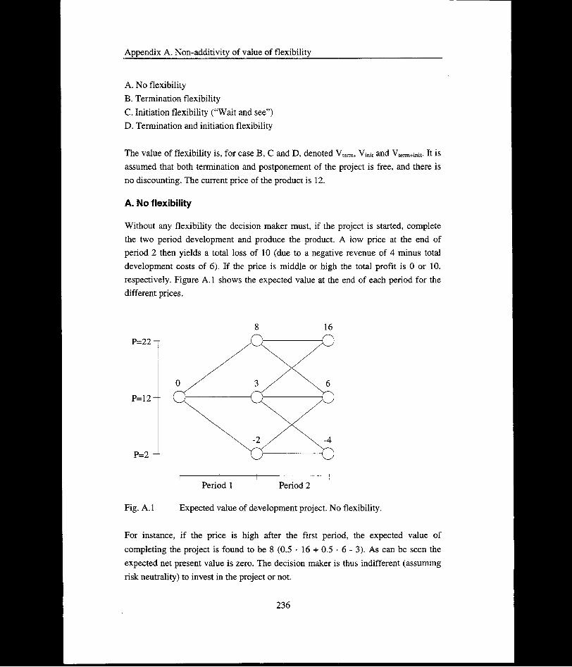
Appendix A. Non-additivity of value of flexibility
A. No flexibilityB. Termination flexibilityC. Initiation flexibility (“Wait and see”)D. Termination and initiation flexibility
The value of flexibility is, for case B, C and D, denoted Vtenm Vini, and VtomH.init. It is assumed that both termination and postponement of the project is free, and there is no discounting. The current price of the product is 12.
A. No flexibility
Without any flexibility the decision maker must, if the project is started, complete the two period development and produce the product. A low price at the end of period 2 then yields a total loss of 10 (due to a negative revenue of 4 minus total development costs of 6). If the price is middle or high the total profit is 0 or 10, respectively. Figure A. 1 shows the expected value at the end of each period for the different prices.
8 16P=22 —
P=12-
P=2 -L
Period 1 Period 2
Fig. A.l Expected value of development project. No flexibility.
For instance, if the price is high after the first period, the expected value of completing the project is found to be 8 (0.5 • 16 + 0.5 6 - 3). As can be seen the expected net present value is zero. The decision maker is thus indifferent (assuming risk neutrality) to invest in the project or not.
236

Appendix A. Non-additivity of value of flexibility
B. Termination flexibility
The decision maker now has the option to terminate the project at the end of each period. Figure A.2 shows the corresponding value of the project. Values at each decision point is the maximum of the expected value from continuing and the value if stopping. It is easy to see that the decision maker only will terminate the project if the sales price is 2 at the end of the second period. If the price is low the flexibility shields the decision maker from a loss of -4, and this provide additional value to the project.
Given this setting the expected value of the project has increased from 0 to 1. The expected value of termination flexibility, Vterm, is thus 1.
P=22 -
P=12-
P=2 -L
Fig. A.2
C. Initiation flexibility
This time we consider a case where initiation of the project can be deferred one period. During the period the price moves up, down or is unaltered with probabilities as given in table A. 1. If the project is started it must be completed.
Figure A.3 illustrates the value of a project with initiation flexibility. A positive net present value (2.5) is here only obtained if the price after the first period is high (22). For the two lower prices the project will not be started. A price increase from 12 to
Period 1 Period 2
Expected value of development project with termination flexibility.
237

Appendix A. Non-additivity of value of flexibility
22 has probability 0.25, and the expected value of the project is therefore 0.625. Correspondingly Vmit is 0.625. Compared to the case without any flexibility the net present value has increased with the same amount. However, for this example initiation flexibility is of less value than termination flexibility.
2.5 8 16
0.625
Period 1 Period 2 Period 3
Fig. A.3 Expected value of development project with initiation flexibility.
D. Termination and initiation flexibility
A combination of the two types of flexibility yields the numbers given in figure A.4. The decision maker can now both delay the start of the project and choose when to terminate it. Given these two options the project will be initiated after one period for prices above 2, and the expected value is 1.25.
238

Appendix A. Non-additivity of value of flexibility
P=22 -r
P=12-
P=2 -
3 8 16
Fig. A.4
Period 1 Period 2 Period 3
Expected value of development project with initiation and termination flexibility.
A.2 The value of added flexibility
The case of combined flexibility is in the example represented by case D, where the project has both termination and initiation flexibility. The value of flexibility (and the expected value of the project) for this case is 1.25. As anticipated this is higher than the values for the two projects with a single type of flexibility. Since the flexibility has no cost the decision maker can not become worse off as more flexibility types are added.
The expected value is however not equal to the sum of the two separate values of flexibility, which amounts to 1.625. Using the terminology introduced above we have
Vterm+init < Vterm + Vjnj_t
Thus value of flexibility is not additive in this simple case. If the project already offers one type of flexibility, the value of adding another flexibility type is lower than if the project does not have any flexibility. As the example shows, the reduction in marginal value can be substantial. For the initiation flexibility the presence of
239

Appendix A. Non-additivity of value of flexibility
termination flexibility reduces its value by 60% (from 0.625 to 0.25). The corresponding reduction in value for termination flexibility is 37.5% (from 1.00 to 0.625).
Even if this example gives clear indication of diminishing value of flexibility, the result can not be generalised. Particularly this concerns the magnitude of the reduction in value. However, it is evident that investment decisions based on separate analyses of flexibility types and their value can lead to gross errors.
240

Appendix B. Upper limit on the correlation coefficient
APPENDIX B UPPER LIMIT ON THE CORRELATION COEFFICIENT
This appendix derives the upper limit on the correlation coefficient p, assuming that
the correlation is due to overlapping information.
B.1 Deriving the limit
Let the number of blocks covered solely by well i be A,., and let Btj be the number
of blocks that are covered by both well i and well j ( i, j— 0,1 i j). A; thus
represents what is called private information to well i, while Bv corresponds to
information common to both wells. If information from a block corresponds to the outcome of a normal random variable with variance c2, the variance of of the
estimated normal distribution based on information from well z", and the covariance (^between the estimate errors, are given as in equation (B.l).
(B.l)
Assuming that A, > 0, i.e., some private information exists, we get
y[g,2(4 + gg)]
241

Appendix B. Upper limit on the correlation coefficient
242

Appendix C. Approximation of the Omstein-Uhlenbeck process by a scaledEhrenfest urn model
APPENDIX C APPROXIMATION OF THE ORNSTEIN-UHLENBECK PROCESS BY A SCALED EHRENFEST URN MODEL
In this appendix an approximation of the general Omstein-Uhlenbeck process is derived based on an Ehrenfest um model. It is shown that the approximation has the desired properties as the length of the time steps of the discretisation approaches zero.
C.1 The Omstein-Uhlenbeck process
The arithmetic Omstein-Uhlenbeck process is defined by (C.l)
dX = -T]-(X-X)dt + <jdz (Cl)
where t) is the speed of reversion, X is the level X tends to revert to (the mean), a
is the standard deviation and dz is the increment of a Wiener process. Since the Omstein-Uhlenbeck process is a diffusion process it can be defined in terms of its drift parameter (C.2) and diffusion parameter (C.3), also termed the infinitesimal coefficients, and the moment condition (C.4).
(C.2)
The diffusion parameter, a2(x,t) = lim -^-£[{AX(r)}2IX(f) = x] = cr2 (C.3)A * ft At *- J
The infinitesimal moment condition,
£[(lAX(r)l)PlX(r) = x] = 0 for some p >2 (C.4)
where AX(r) = X(t + At) -X(t).
243

Appendix C. Approximation of the Omstein-Uhlenbeck process by a scaledEhrenfest urn model
C.2 Approximation by an Ehrenfest urn model
Karlin and Taylor (1981), p. 170, demonstrate that the Ehrenfest urn model can be used to approximate a standardised Omstein-Uhlenbeck process, i.e., a process with 7? = 1 and <7 = 1, by considering a limiting urn process. The limiting process is
derived as follows.
Assume that the number of particles N in the urn model is increased and, at the same time, At is decreased such that N ■ At = 1. A unit of time in the (new) rescaled process will then roughly correspond to N transitions in the original process, while a unit change in the rescaled process will be similar to a change of order V/V in the
original process. Now let F(t) denote the (approximate) rescaled process that
measures deviations from its mean value N. Y(z) is then given by
r( t) =X([At])-A
■JW (C.5)
As the number of particles approaches infinity (N —» <== ), the limiting process Y(t)
will satisfy the infinitesimal coefficients (C.2) and (C.3) and the moment condition (C.4) of the Omstein-Uhlenbeck process with parameters t] = 1 and <7 = 1.
By showing that the general Omstein-Uhlenbeck process (eq. (C.l)) can be transformed into a “standardised” process with r\ = 1 and <7 = 1, we can utilise the
result from Karlin and Taylor to derive the um approximation for the general process. The transformation is carried out in two steps; first the mean reverting factor is “standardised” by a change of the time scale, thereafter the variance is “standardised” through scaling. To ease the exposition it is assumed in the further that the mean of the process is zero.
With X = 0 the general Omstein-Uhlenbeck process is dX = -r\Xdt+adz ■ Set
V(t) = Xj^j/ j. We then get for the increment V(t) - V(0)
244

V'(0I = A'fOj
n
Appendix C. Approximation of the Omstein-Uhlenbeck process by a scaledEhrenfest urn model
where z(t) = ^frj ■ is a standard Brownian motion (cf. Karlin and Taylor
(1975), p. 351), hence, dV --Vdt-¥-^=dz .
= /- V' X (u)du +
= |-V(^ + -^£(t)
Now define W{t) = -V{t). This yields
dW{t) = — -dV{i)o
— 3^1. (_ Vdt) + dz
o= -Wdt+dz
W{t) is thus the “standardised” Omstein-Uhlenbeck process, where
From Karlin and Taylor (1981) we know that T(t), (eq. (C.5)), approximates the
standardised Omstein-Uhlenbeck process. The general Omstein-Uhlenbeck process
will then be approximated by the process Y(r)
245

Appendix C. Approximation of the Omstein-Uhlenbeck process by a scaledEhrenfest urn model
(C.6)Va-V?!
A unit change in the approximating process Y(t) corresponds to a change of order
——— in the general process X{t), while a unit of time in the approximating
process corresponds to N ■ 77 transitions in the general process. Let h be the unit size
of the particle in the rescaled urn model, and As be the time between transitions. The approximating Ehrenfest urn model is then given by eq. (C.7) - (C.9).
(C.7)
(C.8)
(C.9)
where (C.9) gives the probability of a transition of a particle (from one urn to the other) in a time interval As.
It can now easily be shown that the limiting process will satisfy the infinitesimal coefficients, (C.2) and (C.3), and the moment condition (C.4) of the Omstein- Uhlenbeck process as the number of particles approaches infinity {N -» =» ).
The probability of a change in deviation from the mean over a time interval As is

Appendix C. Approximation of the Omstein-Uhlenbeck process by a scaledEhrenfest urn model
PrjAF = ±-j=\Y{x) = y j = Pr{AX = ±11 X([iVrjT]) = x)
= P^AX = ±11 X([M?t]) = N+
"T,
_ 1T y-Jn2 2o4n
N+y1
'2N
where AF = AF(t) = F(t + As) - F(t) . This yields
The drift parameter,
/i(y,r) = ^im^^-£[AFlF(T) = y]
= lim —Ask) As
i y-Vn
- lim — AsioAsL N
•JN-Tj (2 2o4n J *JN r]
y
1 , yjn2 2o4n
= -7]y
The diffusion parameter, cr2(y,T)
°2{y,t)= lim -J-£[{AF}2!F(T)=yAsioAs LL J
= lim —AsiO As
CT2 CT2N-t] (2 2o4n j n-h 2 2(7 VA J
= dm —Ask) As N-T]
= o 2
247

Appendix C. Approximation of the Omstein-Uhlenbeck process by a scaledEhrenfest um model
The infinitesimal moment condition (p = 4),
lim -^-E[lAyi4IF(T)=yla4()As
= lim —<r4 fi rVU CT4
-7?: ^2 2crViVy ' N2 -if (2 ' 2cr Viv Jlim —
Arif) As TV'= 0
The calculations thus strongly indicate that the limiting process converges to an Omstein-Uhlenbeck process in the limit, and this is indeed the case (cf. Karlin and Taylor (1981)). Approximation of the general Omstein-Uhlenbeck process by use of a properly scaled Ehrenfest um model will therefore yield consistent limiting behaviour.
248

Appendix D. Approximation error
APPENDIX D APPROXIMATION ERROR
The suitability of any approximation is determined by its ability to mimic the original process. In this appendix the approximation error of the proposed Ehrenfest um model is assessed. The assessment shows that the approximation yields acceptable results.
D.1 The error of the approximating process
The quality of the approximation of the Omstein-Uhlenbeck process by use of an Ehrenfest um model can be measured by the deviations in expected value and variance. In addition to the desired limiting behaviour (see appendix C), the error of the approximation should be as small as possible.
Let I be a stochastic variable that follows an Omstein-Uhlenbeck process (eq. (D.l)), and denote by X(r) the value of X at time t. For simplicity we assume that
the mean X = 0. With a current value of X(0), the expected value and variance of
X(t) are given by equation (D.2) and (D.3).
dX — —7] ■ (X — X )dt + adz (D.l)
E[x(t))=X( 0)-e~2nt (D.2)
(D.3)
where 77: speed of reversion
X : mean (= 0)<7: standard deviationdr. increment of a Wiener process
Now, assume that X instead follows the approximating Ehrenfest um model, with (one step) transition probabilities given by equation (6.15). The expected value and
249

Appendix D. Approximation error
variance for the approximating Ehrenfest um model is then found in a straightforward manner
INE[Xn\X0=x] = JJpf)-xj (D.4)
(D.5)
where Xn : value of X at stage n
2N: total number of particles in the urnsp\f: n-step transition probability from i to j. (pf1 - p(Xn = xj IX0 - x;,))
Xj: value of X corresponding to state j
Figure D. 1 and D.2 compares, respectively, the expected value and variance given by the Omstein-Uhlenbeck process and three approximations. Both figures are based on a reverting factor, p, of 0.1 and a standard deviation, a, of 2.
The maximum approximation error for the expected value is obtained for X0=xk, k = 0,2N, i.e., if the initial value of X is at one of the extremes. Since the
extreme points are functions of N, three pairs of lines are drawn. These correspond (from bottom to top in figure D.l) to the expected value for the Omstein-Uhlenbeck process and the approximation for N = 5, 10 and 20, respectively. For all approximations the expected value is slightly below the value for the Omstein- Uhlenbeck process. The deviation is, however, minor. It should be pointed out that the difference between the expected value for the Omstein-Uhlenbeck process and the approximations will diminish as the time increases above the years shown in the figure. (The expected value goes to zero as t goes to infinity for both the Omstein- Uhlenbeck process and the approximations.)
250

Appendix D. Approximation error
N =2025 -
Ornstein-UMenbeckApproximation
N = 10
N = 5
Figure D. 1 Expected value of the Omstein-Uhlenbeck process and the approximating Ehrenfest um model, tj = 0.1, <7 = 2.
The variance is calculated for an initial value of X equal to the mean
(X(0) = X = 0). From figure D.2 we see that the approximation error increases up to
t in the range of 4 to 5. Thereafter the deviations between the Omstein-Uhlenbeck process and the approximations decline. Maximum approximation error for the approximation with IV = 5 is 16.2% (t = 4), while the corresponding figures for N= 10 and N = 20 are 7.8% and 4.3% (both for t = 4), respectively.
251

Appendix D. Approximation error
----- N = 5- - N = 10
N = 20Omstein-Uhlenbeck
Figure D.2 Variance of the Omstein-Uhlenbeck process and the approximating Ehrenfest um model, t? = 0.1, <7 = 2.
252

Appendix E. Action space
APPENDIX E ACTION SPACE
The action space consists of 32 actions numbered from 0 to 31 as shown in table E.l. Concepts are identified by initial capacity and optional capacity increments (initial capacity / optional increment). For instance, concept choice (0/1) means a platform with initial capacity level of 0 and the possibility of a 1 step increment of the capacity at a later stage.
Tab. E.l Action space.Action Description Related
phase*-1
Wait and see E, C,P0 do nothing
Drilling of exploration wells E1 drill exploration well cluster
Concept choice + (pre-)drilling of production wells C2 choose concept (0/0) + drill one well cluster3 choose concept (0/0) + drill two well clusters4 choose concept (0/1) + drill one well cluster5 choose concept (0/1) + drill two well clusters6 choose concept (0/2) + drill one well cluster7 choose concept (0/2) + drill two well clusters8 choose concept (1/0) + drill one well cluster9 choose concept (1/0) + drill two well clusters10 choose concept (1/1) + drill one well cluster11 choose concept (1/1) + drill two well clusters12 choose concept (1/2) + drill one well cluster13 choose concept (1/2) + drill two well clusters
Drilling of production wells P14 drill one well cluster15 drill two well clusters
253

Appendix E. Action space
Installation of extra capacity P16 increase capacity by 1 step17 increase capacity by 2 steps
Production P18 produce maximum
Drilling of production wells + installation of extra capacity P19 drill one well cluster + increase capacity by 1 step20 drill one well cluster + increase capacity by 2 steps21 drill two well clusters + increase capacity by 1 step22 drill two well clusters + increase capacity by 2 steps
Drilling of production wells + production P23 drill one well cluster + produce maximum24 drill two well clusters + produce maximum
Installation of capacity + production P25 increase capacity by 1 step + produce maximum26 increase capacity by 2 steps + produce maximum
Drilling of production wells + installation of capacity+ production P
27 drill one well cluster + increase capacity by 1 step + produce maximum
28 drill one well cluster + increase capacity by 2 steps + produce maximum
29 drill two well clusters + increase capacity by 1 step + produce maximum
30 drill two well clusters + increase capacity by 2 steps + produce maximum
Abandonment E, C,P
31 abandon project
*) E: exploration, C: conceptual study, P: production
254