the vapor-liquid equilibrium and related properties of · the vapor-liquid equilibrium and related...
TRANSCRIPT

THE VAPOR-LIQUID EQUILIBRIUM AND RELATED PROPERTIES OFETHANOL, CHLOROFORM MIXTURES
byC. LAWRENCE RAYMOND
B.S. Union College1932
M.S. Union College1933
SUBMITTED IN PA.RTIAL FULFILLMENT OF THE REQUIHEMENTS FORTHE DEGREE OF
DOCTOR OF PHILOSOPHYFROM THE
NASSACHUSETTS INSTITUTE OF TECHNOLOGY1937
/1 _
v
.' I~.
Signature of Chairman of Departme;Committee on Graduate Studen
/ (/
Signature of Author,Department of Chemistry, May 13, 1937Signature of Professor
in Charge of Research _

Acknowledgment
To Professor George Scatchard for his guidance andvaluable advice, to Mr. Henry~. Wayringer for his ingenuityin constructing apparatus and to Dr. Scott E. Wood for manyhelpful suggestions. I wish to express my sinoere apprecla-tion.

Table of 'ContentsPart I
Section(1) Introduction(2) Apparatus
EquilibriumThermocouplesManometer System
(3) Materials(4) Density of Ethanol. Chloroform Mixtures(5) Experimental(6) Results and Calculations
Vapor Pressures of Ethanol and ChloroformExperimental results on the equilibrium
isotherms of the MixturesPerfeot Gas law correctionsCalculated chemioal potentials
and free energies of mixingCalculated Heats and Entropies of
mixing at 45°C.(7) Discussion(8) Summary
Part II
(1) Historical SurveySupplementary References
Page1
4
4
7
9
11
1415181821
2936
41
42
46
1
8

Table of Contents (2)
Section(2) Supplementary Details of Equilibrium Still(3) Potentiometer System
Standard CellsGalvanometer
(4) ThermocouplesCalibration of 20 Junction Thermo-
coupleCalibration of single Junction thermo-
couples(5) Manometer system
McLeod Gauge CalibrationSoale calibration
(6) Pressure CorrectionsCapillary depressionThermal expansion and oalibration
of the scaleStatio headTemperature of Hg. and standard
gravity(7) Prooedure in pressure measurements(8) Materials (oontinued)(9) Density Measurements
Pycnometer Calibrations(10) Bibliography(II) List of Figures(12) Notebook Referenoes(13) Biographical sketch
Page10141515
20
24
25
30
31363740
4043
46
515355
58
59
6061

PART I

-1-
Introduotion
Equilibrium pressure, temperature, vapor-liquid oompo-sition measurements for binary liqUid systems are of valuefrom two points of view. Measurements of this type give theexperimental background for the oonsideration of the problemof the thermodynamics of binary systems. Also these dataarenecessary in the design of fractionating apparatus for theseparation of liquid mixtures into their oomponents.
From the vapor pressure, temperature and vapor oomposl-tion1values for the chemioal potentials of each of the compo-nents in a mixture and the free energy change for the change1n state of mixing the pure oomponents can be derived. Valuesof the changes 1n entropy and heat content for this changein state can be calculated from the variation of the freeenergy change with temperature. Values of these thermody-namic functions must be known from experiment to verify thevalidity of the statistical development of the theory ofbinary liqUid solutions.
The exact calculation of the chemical potentials canbe made only if the deviations of the vapors from the idealgas laws are known. The Gibbs-Duhe~l) equation relating thevapor and liquid oomposition offers a means for estimatingthese deviations.
The experimental problem of measuring the equilibriumpressure, temperature and compositions of the two phases has

-2-
one outstanding difficulty; tne determination of the vapor(2)phase composition. Cunaeus attempted a direct analysis of
the vapor phase in the gaseous state in a purely statio systemby measuring the refractive index. The lack of precision ofthis method of analysis of a gas mixture accounted for thefailure of this apparatus. Other methods previous and sub-sequent to this depended on condensing the vapor in sufficientquantity for analysis in the liquid state. In a distillationmethod such as was employed by Zawidsk13) vapor is constantlybeing removed from the system by distillation. At no timeduring the process is the system at equilibrium. In practicalcases where the quantity of liquid is finite, this continuousremoval of vapor at constant pressure causes continuouschanges in the temperature and compositions of both the liquidand vapor phases. The accuracy of this simple distillationmethod depends on the ratio of the volumes of the condensedvapor and residual liquid, the rate of distillation and thenature of the heat source. The results of such a method canunder the best experimental conditions be only approximate.
(4 )Later Rosanoff, Lamb and Breithut suggested a means toavoid these difficulties which involved attaining equilibriumbetween the liquid phase and a vapor of constant compositionsupplied continuously from an external source. At equilibriumas much of the vapor can be condensed as desired without dis-turbing the equilibrium conditions.
Sameshim~5,6) introduced a continuous distillation

-3-
method which is basically a flow process. In this methodvapor is continuously condensed, but it is not removed fromthe system. After a portion of the distillate has beentrapped the overflow feeds back into the liquid. If duringthe distillation process the temperature, the composition ofthe system and the volumes of the liquid and condensed vaporare constant, a steady state will be produced where the pres-sure and the composition of each phase will be invariant withtime. An apparatus operating on this principle will be termedan equilibrium still.
In such a still equilibrium between the liquid and vaporphases must be produced at the point where the temperatureand pressure are measured; that is both liquid and vapor mustbe continuously in contact with the thermometer. The suocess-ful operation of this apparatus requires that the composition
.of the condensed vapor and residual liquid be equal to thoseexisting at the point where equilibrium is produced.
An apparatus based on the principle of the equilibriumstill has been constructed to measure the liquid vapor equilib-rium isotherms of binary mixtures of volatile, completely mis-cible liquids. Three equilibrium isotherms have been determinedfor the ethanol-chloroform system.

-4-
Apparatus
The apparatus consisted of three principal parts, theequilibrium still, a manometer system for pressure measure-ments and thermocouples for temperature measurements.
The equilibrium still was similar to the one described7by Chilton. Several improvements were added, and the ap-
paratus arranged to operate over a pressure range of 100 m.m.of Hg. to 1 atm. rather than constantly at 1 atm. A scaledrawing of the still is shown in figure (1). The still isblown in one piece and is entirely of pyrex glass. The threeprincipal parts are the liquid boiler (B), the condenser (D)and the distillate trap (0). The liquid boiler is constructedof two concentric cylindrical vessels which form an outerliquid vessel (E) and an inner liquid vessel (F). Heat isapplied at the bottom of the outer vessel by means of ashielded, circular gas burner.
It is desired that equlli brium take place a.round thelower portion of the thermometer well (I). A glass spiralis wound around the well to hold an appreciable volume ofliquid in contact with it. A mixture of vapor and liquidis lifted from the inner liquid vessel (F) by the pumpingdevice (H) and discharged over the spiral surrounding thethermometer well. The liquid in the inner vessel is heatedby a jacket of vapor produced in the outer boiler. The vapor"is conducted to the bottom of the inner vessel through tube(G) where as it escapes it bubbles through the liquid and

IOCM.
D
M
p
if
~Jo I, II II II I
iIII
A
B
G
FIG. I
EQ.UILIBRIUMSTILL

operates the pumping device. The outer boiler is maintainedat a slightly h~ pressure than the inner one depending onthe level of the liquid in (F). Consequently the vapor pro-duced in the outer boiler is slightly super heated. Thisvapor jacket prevents condensation on the inner walls of theinner vessel and protects the thermometer well from externalinfluences. The vapor leaving the inner liQuia boiler entersthe condenser (D), and the distillate conducted to the bottomof the distillate trap (C). The overflow enters the bottomof the liquid boiler through tube (L).When a steady state exists no condensation or vaporiza-tion occurs in the inner liquid vessel. Then, if the vaporafter leaving the liquid in the inner liquid vessel does notchange in composition until it is condensed, the compositionsof the distillate and the liquid remaining in the inner ves-sel are equal to the equilibrium compositions.
To minimize fractionation effects resulting-from re-flux of the liquid the top of the inner boiler was providedwith a flanged lip the lowest point of which emptied intothe distillate trap. The distance between this flange andthe ringseal joining the outer and inner liquid boilers wasmade as small as possible to reduce the exposed surface.
The relative height.G of tube (G) and the distillateoverflow tuh~ (L) were adjusted so that it was possible toincrease the pressure in the system quite rapidly withoutsucking over the contents of the inner liquid boiler through

-6-
tube (G). The gas necessary to fill the outer liquid boilerentered entirely through the distillate over flow tube.
The tube (K) connecting the condenser outlet with theupper part of the distillate trap was for the purpose of equal-izing the pressure over the surfaces of the condensate and toallow the passage of gas from the oondenser into the liquidboiler. The tube was mounted on an angle slanting downwardstoward the condenser outlet to prevent any distillate fromentering the trap at this point.
The inner liquid vessel and the distillate trap wereprovided with tubular openings which were sealed by means ofground glass stoppers for removing samples of the liquid anddistillate for analysis. A third tube also provided with aground glass stopper was mounted directly above the distillateoverflow tube to afford easy access to the outer liquid boiler.The grindings of these stoppers were carefully polished and theuse of lubricant was not necessary.
The condenser (D) was constructed in a manner to furnishboth inside and outside condensing surfaces. The outside sur-face was cooled by means of a surrounding lee Jacket and theinside surface by means of water precooled to ice temperature.The tube (X) at the top of the condenser is a pressure con-nection leading through a liquid air trap to the manometersystem. The condenser was mounted in a vertical positionwhich allows the lighter gas filling the manometer system

-7-
to float above the heavier condensing vapors and gives a sharpvapor gas interface. It is then certain that no gas is mixedwith the vapor in the still. A sharp interface is also neces-sary for the existence of constant pressure in the system.
The condenser was designed to have as large a condensingsurface as possible and yet have the volume per unit lengthsmall. This is desirable so that fluctuations in the level ofthe condensing vapor in the condenser caused by slight changes1n rate of boiling etc. will not produce any appreciable pres-aure change in the manometer system. The relative volumes ofthe manometer system were such that a Change of 2 m.m. 1n thevapor level produces a change of 1 part in 100,000 in the pres-aure of the system.
The thermocouples consisted of twenty ropper-constant~nJunctions conneoted in series. Each junction head and eachlead wire were indiVidually insulated with four coa~s of bake-lite enamel. The twenty insulated thermo Juncttons were boundtogether with silk thrend and mounted in a rigid bakelite sup-port. The hot and cold junctions extended downward parallelto each other a distance of 6 1/2 inches out of the bakelitesupport. The cold Junction was surrounded by 8 mm. glasstubing filled to a depth of 4 1/2 inches with mineral 011which served as a conducting medium for heat transfer. Thelee point temperature (ooC.) was used as a reference temper-ature in all thermocouple measurements.

-8-
The construction of the hot Junction is shown in fig.(1). The junction leads are conduoted away from the bakelltesupport through the glass tube (M) for a distance of 2 inches.The remaining 4 1/2 inches of lead wire and the junction heads(p) were tightly wound with silk thread and impregnated withbakelite enamel. The junction heads were given the addedprotection of a shield of two turns of silk tape also impreg-nated with bakelite enamel. The hot junction when inserted1n the thermometer well extends to the bottom, and the clear-ance between the Junotion heads and the side walls is about1/16 inches on each side. The thermometer well was filled toa depth of 3 3/4 inches with mineral oil. With the hot junctionconstructed in this manner th~ ratio of the heat conductionalong the leado in a vertical direction to the conduction tothe.surface of the thermometer wpll 1n a horizontal directionwas small enough to make the thermocouples relatively insensi-tive to depth of immersion at the operating depth.
Electromotive measurements were made with a Leeds andNorthrup type "K" Potentiometer. The potentiometer systemwas sensitive to a change of 1 microvolt. A temperature dif-ference of lOC. produced an E.M.F. of .8 millivolts. Hence atemperature difference of .001°0. could be detected. Assumingthe E.M.F. of five Epply saturated cadmium cells remained con-stant, temperatures could be reproduced to .001°0. The absolute
+value of the temperature ~asuncertain to - .OloC.The thermocouples were calibrated by oomparing with a
25 ohm platinum resistance thermometer over a range of 25°C.

-9-
to 100°C. The resistance thermometer had been recently cali-(8,9)brated by other workers in this laboratory. As an independent
check the thermocouples were calibrated in the equilibrium stillby the vapor pressure curve of water over a range of 60°C. to100°0. The relation between the vapor pressure end temperature
(10)for water of Smith, Keyes and Gerry was used to calculatethe temperature from the observed pressures. These two inde-
+pendent calibrations agreed to - .010C.The manometer system is shown schematically in fig. 2.
The system was filled with nitrogen when measurements were madeon alcohol and chloroform vapors and helium for thoreon watervapor. Pressures were measured with a mercury manometer (A)
in conjunction with a cathetometer and graduated scale. Thescale was a two meter invar bar graduated in millimeters andwas calibrated by the U.S. Bur~au of Standards in Oct. 1934.The mercury column was thermo stated by means of an air bath)and the mean temperature of mercury could be determined to+- ~O~oC. The observed mercury heights were reduced to pres-sures in m.m. of Hg. at OOC. and standard gravity and correctedfor capillary depression, st~tic head and celibration and ther-mal expansion of the scale. The uncertainty in the absolute
+values of the pressure was - .01 m.m. of Hg. at a pressure of1 atm.
The manometer (B) is connected in parallel with the mainmanometer and is used for rough pressure measurements. The

_-
--
--
--
--
--
--
-.
-J
(
w
--------
-------------------------------
------------
..-----------------------1
I:II:IIIII
<{
:I--------------
----------------------------------------------------------
mo
-Io0>
o
,------------
-----------
-----
---------------,I
II
II
II
:I
II
IL
_--,-1=~~-'-'
iIII:Ii!1.-
.1
cr.
L-----------ri1
'fu--
U.-
---~
IW_
--
I«>
JJ~11'/
o~
-10-
barostat (D) consisted of a 90 liter thermostated volume forthe purpose of minimizing pressure fluctuations caused bytemperature changes in the leads and changes in vapor levelin the still condenser. The connections labeled H in fig. 2lead to a Hyvac oil pump. The pressure in the system wasregulated through stopcocks (V) and (Q). By opening stopcock(Q) small quantities of gas could be admitted to the systemby noting the pressure dropin a 250 cc. bulb by the manometer~I). In this manner the pressure could be controlled 1n the
+system to -.01 m.m. of Hg. Tank nitrogen and helium were ad-mitted to the 250 c.o. bulb through stopcock (8) after passingthrough drying tubes.

-11-Materials
Ethanol: The source of ethanol was the commercial grade ofabsolute alcohol. The commercial product was purified by the
(12) (13)method recommended by Castille and Henri . Harris found(14 )that absolute alcohol from the same source as used in
this work after p~rification by the Castille and Henri methodhad a benzene content of less than .001% by weight and analdehyde content of less than .02%. The vapor pressures of55°C. of samples of three separate purificationc were279.820 m.m., 279.902 m.m., 279.815 m.m. Densities of thedifferent purified samples indicated the presence of .05%to .1% of water. The pure alcohol was stored in 100 c.c.glass stoppered bottles.Chloroform: Chloroform is unstable in the presence of airand oxidizes to form carbonyl chloride and hydrochloric acid.This decomposition is catalysed in the presence of light,but 1s stabilized by the presence of a small amount of ethanol.The principal impurity in the ordina.rygrade of purifiedchloroform is about 1% of ethanol which has been added forthis purpose. This alcohol was removed during the purifica-tion process suggested by Timmerman and Martln(15). Approx-imately 1% by volume of ethanol was added to the purifiedchloroform.and the mixture stored in the dark in 100 c.c.glass stoppered bottles. Pure chloroform ~ns used only inthe measurement of its vapor pressure curve and the densi-ties of chloroform, ethanol mixtures. In these cases

-12-
measurements were made as rapidly as possible after purification.It was found that the density of a sample of pure chloroformincreased only .03% after standing in the light for a periodof 1 month. Since the decomposition products of chloroformare volatile, they should gradually be eliminated during theprocess of vapor pressure measurements made by the distilla-tion method. The vapor pressures at 55°0. of samples of theproducts of three different purifications were 617.772 m.m.,617.903 m.m., 617.837 m.m.N~nometer Mercury: The ordinary grade of redistilled mercurywas purified further first by the electrolytic process andthen by two successive distillations. The first distillationwas carried out under a pressure of 20 m.m. of air, and thesecond under vacuum.

-13-
Density Measurements
Analyses of the liquid and distillate samples were madeby means of density measurements. The densities of the mix-tures were determined in glass pycnometers at 25°0.
Mixtures of chloroform and ethanol of known compositionwere made up by weight in glass weighing bottles and theirdensities determined. The results of these measurements aregiven in table I. The composition (Z) in mole fractions wasexpressed as the deviations Z - Z(calc.) from a quadraticfunction of the specific volumes.
Z (calc) a= - 3.43407 + 6.8893lV - 2.67566V
The deviations of the observed values of Z from the valuescalculated from this equation are plotted as ordinates infigure 3 against the specific volume as abscissae. The meas-ured points are indicated by circles and.fallon a smoothcurve within .03 mol %. The points indicated by crosses in
(11)figure 4 are the deviations of the measurements of Hirobefrom the given equation. The density method is particularlyapplicable to the analysis of chloroform, ethanol mixturesbecause of the large spread between the densities of thepure components. Analyses were made by use of the deviationcurve, and the maximum lJnce~talnty in composition is .05 mole %.

-14-Table I
Specific Volume of Ethanol, Chloroform Mixtures25°C.
Weight Frac. Mole Frac. Density Specific D (Z obs. -Z calc.;Ethanol Ethanol (Z) Volume
~~~-~-~~~~-~----~~-~~~~~~~~~-~--~-~--~--~----~-------------~-~~-------0 0 1.47955 .67588 .00000
.03371 .08293 1.43640 .69619 .01759
.06581 .15443 1.39796 .'11533 .02950
.08652 .19713 1.3'7477 .72739 .03566
.14834 .31108 1.30804 .76450 .04208
.16509 .33889 1.29163 .77422 .04297
.27136 .49122 1.19656 .8~573 .03649
.35914 .59230 1.12584 .88823 .01806
.41301 .64589 1.08789 .91921 .00803
.59394 .'19131 .973'14 1.02697 -.02780
.64787 .82668 .94561 1.05752 -.03251
.72669 .87330 .90360 1.10668 -.03990
.78558 .90474 .87544 1.14228 -.03950
.84801 .93525 .84774 1.17961 -.034251 1 .78562 1.27288 -.00002
Z(ca1c.) = -3.43407 + b.88931V - 2.67566V3

(~
~
~i
~c
III$P
I
/I
/' vv-----;-
/IIII
/I
VV+
-I../
VV
V;4f::~
~~~
III..J
1\I0
~>uu.u
ow
C\ja.
_lI'I
01'1
9o9oO!
o~ot-:
NC!-q
oNq
..q

-15-Experimental
A mixture of chloroform and ethyl alcohol in the properproportions to give approximately the desired final equilibriumcompositions was introduced into the still. The total volumeof liquld mixture required wac about 157 c.c. of ?!hlch 85 c.c.was placed in the inner boiler, 45 c.c. in the outer boilerand 27 c.c. in the distillate trap. The volumes in the innerand outer liquid boilers changed somewhat during the opera-tion of the still. The pressure was reduced through stopcocks(U) and (V) until the liquid in the still just started to boil.Stopcock (V) was then closed, and gas from the manometer system,in Which the pressure had been adjusted to approximately thedesired value, was slowly admitted to the still by partiallyopening stopcock (T). When the pressure in the still and themanometer system became equal, stopcock (T) was fully opened;and heat was ~pplted at the bottom of the liquid boiler. Theliquid was allowed to boil vigorously for a time to allow thevapors to flush out other gases. The heat was then reduced tothe point where uniform boiling occurred.
The potentiometer system was adjusted to the E.M.F.corresponding to the required temperature; and throughoutthe time a steady state condition was being attained, thetemperatu~e was maintained as constant as possible by regula-tion of the pressure. The criterion for a steady state was theexistence of constant pressure and constant temperature overan interval of at least 5 minutes. The time necessary to

-16-
attain a state very near to the equilibrium or steady statewas usually about 20 minutes after boiling first occurred.The actual equilibrium point is then reached only after verycareful pressure adjustment. The total time required to reachthe steady state condition was from a minimum of 45 minutesto a maximum of 2 1/2 hours depending on the initial composi-tions and the region of temperature and pressure.
At the equilibrium point a temperature drift towardshigher temperature occurred. The value of this driftreached a maximum in the middle of the concentration rangeof .0030C. per minute and decreased to a minimum value ofless than .001°C. per minute in the Vicinity of each of thepure components and the constant boiling mixture. Since atthe condensing temperature (ooC.) the vapor pressure of chloro-form is 5 timan that of ethanol, this drift was attributed tounequal rates of escape of the vapors of chloroform andethanol through the condenser. It was estimated by the vol-ume of liquid condensed in the liquid air trap that loss ofmaterial through the condenser had a maximum value of .5 c.c.per hour and was usually much smaller than this.
When a steady state was reached the manometer system wasshut off by closing stopcock (T). The heater was extinguished,and nitrogen gas was admitted to the still as rapidly as pos-cible through stopcocks (U) and Q) until the internal pressureindicated by manometer (I) attained a value slightly in excessof 1 atm. The pressure was then measured on the main manometerby determining the heights and levels of the menisci and the

-17-
temperature of the mercury and invar scale. Samples of theliquid and distillate were removed for analysis from the in-ner boiler and distillate trap by means of ice jacketedpipettes. Since the operating pressures in the wo~k on mix-tures were less than 655 m.m. of Hg. the rapid increase inpressure in the still to 1 atm arrested distillation immedi-ately.
The still was also used to determine the vapor pressure,temperature curves for pure chloroform and ethanol. Theprocedure was similar to that described for mixtures exceptthe pressure was read while the still was actually in opera-tion without closing off the manometer system. The pressuredrift in the system with time was very small and could notbe detected over the time necessary for a pressure measure-ment. Pressure fluctuations about a mean value caused bychanges 1.nthe vapor level 1n the condenser were small andin low pressure ranges where irregular boiling occurred inthe still reached a maximum value of .02 ID.m. of Hg.

-18-
Results and Calculations
The measured values of the vapor pressures of pureethanol and chloroform at several temperatures are given inTable II. The pressures given are average values for severalobservations. The vapor pressures for both substances are some-what lower than the published values (Int. Cri~. Tables, Vol. III).For ethanol the difference between tne observed values and pub-lished values ranges from -0.4 m.m. to -1.4 m.m. except at 75°0.where the difference is +0.4 m.m. For chloroform the differ-ences are much greater and .rangesfrom -4.B m.m. to -9.5 m.m.Since ethanol and chloroform form azeotropic mixtures ~f max-imum vapor pressure with the substances most Itkely to be pres-ent as impurities, low values of the vapor pressure would beexpected to be the most probable.
Three vapor-liquid equilibrium isotherms were measuredfor mixtures of the two pure components at 35°0., 45°C., and55°C.
Table IIVapor Pressures of Chloroform and Ethanol
35.4045505560657075
Pm•m• (Ethanol)102.78134.091'12.'16221.18279.86351.32438.36542.09666.49
Pm.m.(Chloroform)295.11360.28433.54519.18617.84730.14

-19-
The experimental results at these three temperatures appearin Tables, III, IV and V. In the following discussion theterms will be defined as follows:
p = total vapor pressure in m.m. of Hg.
x = mole fraction of ethanol in the liquid.y = II " tt II " " vapor.
EJ.ll= excess chemical potential of ethanol.E " II " II chloroform.JJ.a =
F E = excess free energy per average mole.xSxE = II entropy II II II
.H E = tt heat content II II "X
A subscript (l) applied to any symbol refers to ethanol anda subscript (2) to chloroform. When the two pure liquid com-ponents are mixed the quantities, J.l,F, H, S undergo correspond-ing changes. The changes in J.lIand J.laon mixing are
JJ.IM= RT In 8.1MJJ.a = RT In aa
whe~e a1 and aa are the activities. E EThe symbols JJ.l and J.larepresent the changes in chemical potential of each componentfor this change in state in excess of the changes that wouldhave taken place if the solution had been ideal and are definedas follows.
M EJ.ll = RT In Xl + JJ.l
M EJJ.a = RT In (I-x) + Ua
E EThe values of JJ.l and JJ.a are hence equal to the RT times

-20-
logarithm of the quantity generally known an the activitycoefficient.
E E EThe symbols Fx , Hx and Sx represent the excess freeenergy, heat content and entropy changes when the mixturecontains a total of 1 mole.
F M M M= XJ.l.l+ (I-x) J..1.ax
F E E E= XJ.l.I+ (I-x) J.l.ax
For ideal solutions the heat of mixing is O. Therefore forany solution
Likewise:
In the first three columns of Tables III, IV and V aregiven the experimental values of P,x and y for the threetemperatures.

-21-Table'III
35°0. IsothermMole frae. CaHsOH
x y P P Y P (l-y) 6 log10Pm.m.------------------------------~-------------~-----------------0 0 295.11 0 295.106 0
.0384 .0586 303.91 1'7.81 286.10 .039614
.0400 .0597 303.69 18.13 285.56 .039797
.0414 '.0615 304.17 18.69 285.48 .041287
.0440 '.0637 304.87 19.42 285.45 .043302
.0685 .0839 306.05 25.68 280.37 .054241
.1517 .1217 306.25 37.27 268.98 .071841
.1577 .1248 305.12 38.08 267.04 .071666
.1735 .1302 305.39 39.76 265.63 .074522
.2254 .1446 303.05 43.82 259.23 .077778
.3217 .16'13 296.93 49.68 24'7.25 .079263
.3815 .1819 291.95 53.10 238.85 .0'18664
.5154 .2188 274.46 60.05 214.41 .068734
.5173 .2203 274.04 60.37 213.67 .068747
.5616 '.2354 267.65 63.00 204.65 .065426
.6078 .2588 255.28 66.07 189.21 .05594
.6155 .2630 253.39 66.64 186.75 .054292
.6773 .2991 236.50 70.'14 165.76 .040868
.6986 .3130 229.24 71.75 157.49 .033700
.7127 .3253 225.06 73.21 151.85 .031330
.7639 .3793 205.68 78.01 127.67 .016962
.8270 .4696 177.60 83.40 94.20 -.005405
.8891 .6115 148.26 90.66 5'1.60 -.018819
.9406 .7657 125.82 96.34 29.48 -.0194'/1
.9458 .7846 123.54 96.93 26.61 -.018741
.9'103 .8'190 113.61 99.86 13.75 -.011915
.9759 .9009 111.31 100.28 11.03 -.010739
.9938 .9746 104.87 102.21 2.66 -.0028801 1 102.78 102.78 0 0

45°C.Isotherm
-22-Table IV
Mole frac. CaHsOH
--~-------_:_------~~:~:_----~_:_----~-~==:~----~-~~~~Q:_--.0 0 433.54 0 433.54 0.0134 .0273 439.89 12.01 42'.88 .017231.0242 .0421 443.07 18.64 424.43 .026252.0323 .0546 445.38 24.32 421.06 .033518.0443 .0681 44B.49 30.52 417.9'1 .041931.0837 .1026 453.'16 40.56 407.21 .060797.0875 .1054 454.02 47.85 406.17 .062167.0900 .1067 454.54 48.45 406.09 .063177.1148 .1217 455.79 55.47 400.32 .070364.1794 .1484 455.56 67.61 387.98 .080818.2852 .1809 448.17 81.07 367.10 .086702.3717 .2046 438.89 89.80 349.09 .087079.4595 .2297 425.28 97.69 327.59 .083435.4860 .2397 420.63 100.83 319.80 .082650.5561 .2660 403.91 107.44 296.47 .075548.5985 .2857 391.51 111.85 279.06 .06~875.6702 .3286 365.07 119.96 245.11 .056645.6884 .3443 355.66 122".45 233.21 .051579.7431 .3940 329.62 129.87 199.'15 .038415.7989 .4605 299.63 137.9B 161.65 .023566.8003: .4634 298.08 138.13 159.95 .022472.8740 .6026 249.92 150.60 99.32 .001555.9288 .7533 214.44 1til.54 52.90 -.004'120.9524 .8283 199.62 165.34 34.27 -.005863.9811 .9284 182.63 169.55 13.08 -.U04509.9843 .9400 180.96 170.10 10.~6 -.003846
1 1 172.'16'172~76 0 0

-23-
Table V55° Isotherm
Mole frac. CaHsOHx y P P y P(l-y) ~ log P---------------- ~~m~ ~~ _
°.0348.0570.0963.1610.2236.2731.3149.3789.4270.5206.6035.6096.6233.6555.658B.7194.7799.8131.8521.8971.9198.9288.9669
1
o.0592.0850.1202.1583.IB19.1990.2143.2361.24'73.2839.3240.3280.3359.3581.3593.4058.4'129.5205.5965.6877.7467.7698.B838
1
617.84626.79644.24650.38653.11650.96646.79641.49632.14623.67599.03569.02566.74560.25545.72543.53508.'18469.41441.04407.90367.01346.8~339.~9306.38279.86
o37.7154'.7978.18
103.39118.41128.71137.4'1149.25154.231'10.06184.36185.89188.19195.42195.29200.46221.9t5229.56243.31252.40259.02261.65270.'"78279.86
617.84599.08589.46572.20549.'12532.55518.08504.02482.89469.44428.973H4.66380.853'12.00350.30348.24302.3224'1.43211.48164.59114.62
87.8778.2435.60
o
o~033488.047420.063634.0'18557.085242.088330.090023.091139.OB9133.084217.075687.0'15315.0'13033.009255.00'1919.055225.043323.032614.024832.010328.006121.005224
-.000652o
The vapor pressure P is plotted against x and y in figure(4). The P-x points are indicated by circles and the p-ypoints by flagged circles. The lowest curve is the" 35°C.
isotherm and the highest curve the 55°C. isotherm. Thisdata shows that mixtures of chloroform and ethanol forman azeotropic system of maximum vapor pressure at the threetemperatures, 35°0., 45°0., 55°0. The composition of theconstant boiling mixture shifts with increasing temperaturetoward higher ethanol content. The compositions of the mix-tures of maximum vapor pressure at 35°C., 45°0., and 55°C.

-23-
Table V55° Isotherm
Mole free. CaHsOHx y P P Y P (l-y ) ~ log P-_________________________~~m~ 10-------------------------------------~-
° 0 617.84 0 617.84 0.0348 .0592 626.79 37.71 599.08 .033488.0570 .0850 644.24 54'.79 589.46 .047420.0963 .1202 650.38 78.18 572.20 .063634.1610 .1583 653.11 103.39 549.'12 .0'18557.2236 .1819 650.96 118.41 532.55 .085242.2731 .1990 646.79 128.71 518.08 .088330.3149 .2143 641.49 137.4'1 504.02 .090023.3789 .2361 632.14 149.25 482.89 .091139.4270 .24'13 623.67 154.23 469.44 .089133.5206 .2839 599.03 1'10.06 428.97 .084217.6035 .3240 569.02 184.36 3H4.66 .075687.6096 .3280 566.74 185.89 380.85 .0'15315.6233 .3359 560.25 1~8.19 3'12.00 .0'13033.6555 .3581 545.72 195.42 350.30 .009255.6588 .3593 543.53 195.29 348.24 .00'1919.7194 .4058 508.'18 200.46 302.32 .055225.7799 .4729 469.41 221.ge 24'1.43 .043323..8131 .5205 441.04 229.56 211.48 .032614.8521 .5965 407.90 243 ..31 164.59 .024832.8971 .6877 367.01 252.40 114.62 .010328.9198 .7467 346.8~ 259.02 8'"7.87 .000121.9288 .7698 339.89 261.65 78.24 .005224.9669 .8838 306.38 270.78 35.60 -.000652
1 1 279.86 279.86 0 0
The vapor pressure P isplotted against x and y in figure(4). The P-x points are indicated by circles and the p-ypoints by flagged circles. The lowest curve 1s the"35°C.
isotherm and the hignest curve the 55°C. isotherm. Thisdata shows that mixtures of cnloroform and ethanol forman azeotropic system of maximum vapor pressure at the threetemperatures, 35°C., 45°0., 55°0. The composition of theconstant boiling mixture shifts with increasing temperaturetoward higher ethanol content. The compositions of the mix-tures of maximum vapor pressure at 35°C., 45°0., and 55°C.

600
400
200
~ 'K~
~~"\
~1\ ,-
\ ~I~ ~ - I
" ~ \1~ - .,..--..._- --~ ""
~~r---o-.
~
I 1\1~
Q, '1
~~
~. - ~ 1\~-- _0
~
~ N\~L~.,.. ~~--- ~,-
~ ~
~~ ~I~~ R>...
'\~
~ \~ "r--...
~ " ~~
~~I~ .....
~~~
o .2 .4 .6FIG.4
.8 1.0
MOLE FRAC. X

-24-
are x = .105, x = .130, x = .155. In the third and fourthcolumns of Tables III, IV and V are given values of Py andP (l-y) which are by definition the partial pressures ofethanol and chloroform. The values of P, P Y and P (l-y) at45°C. are plotted against x in figure (5). The P y curvecrosses the Raoult law line. This crossing is more pronouncedat 35°C. and becomes less noticeable at 55°0.
The values of the chemical potentials can be calculatedfrom the total vapor pressure and the vapor composition ifthe vapors are assumed to obey the perfect gas laws. If forreal vapors the deviations from the gas laws are known thenthe exact calculation can be made. If the equation of statefor mixtures of the vapors of a two component system is ex-.pressed as
VN
RT= p
or if S = 2~12 - ~l~~
V RTN ~ -p--- + ~l Yl + ~2 Y2 + S Yl Y2
where 5 is the deviation of the volume of the mixture fromaditlvity, then the changes in chemical potential on mixingin the liquid (~M) for each component at constant pressureeaual to final vapor pressure above the mixture are
M Py 2~l = RT In ---- + (~l-Vl)(P-Pl)+SP (l-y)
PI
= RT In ~i~:Y) + (~2-V2)(P-P2) + SPa
P 2Y

I
I--1-..-I
-L---+-----M.------+------ii
~---I--+---+-~~-+--~~i
400 ~~~----+---+-----+----+~~--+----+---t-----;
200 ..---+---
o .2 .4 .6 .8 1.0
FIG.5MOLE FRAC. X

-25-
where PI and Pa are the vapor pressures of the pure component A
at temperature T and VI and Va are the molal volumes of thepure liquids.
The Gibbs-Duhem equation, relating the value of thechemical potential of one component to that of the other, of-fers a means of estimating these deviations of the vapormixtures from the p6~fect gas laws by the use of vapor-liquideauilibrium measurements. Since the values of these deviationsare small, equilibrium data of a comparatively high degree ofaccuracy are required to carry out this calculation success-fully. The Gibbs-Duhem equation for a binary system is
x d~l + (I-x) d~a = 0
By differentiating the expressions for 1J.1M and. J..1aM at constant
T and considering P and y variables and 8ubstituting,theabove equation takes the following form
y (1-y) ~-~~-~- = -(x-y)dy
For simplicity let the second factor on the right hand sideof the expression equal R and let the equation be written
y (l-y)d In P
dy= -R (x-y)
d In PThe quantities (x-y) and y(l-y) ---------
dycan be derived from the experimental data. If the data

-26-
represents eauilibrium accurately, the difference in thevalues of these two quantities is caused entirely by the devia-tions of the vapors from the perfect gas laws. By determiningR at different values of y so that the above equation is satis-fied, values of ~l, ~2 and S can be estimated.
In order to carry out this calculation it is necessaryd In Pto obtain values of ------ These slopes were obtained bydy (16)
numerical differentiation using the Rutledge method forfive points. The method assumes that essentially the desiredslope is given by the slope of a biquadratic passed throughfive evenly spaced, adjacent points including the point atwhich the sloped desired. The symetrical case vrhere thepoint in question is the third of the five adjecent pointswas used in this work.
The differentiation was not carried out directly onthe log P-y curve but on the b log P-y relation. ~ log P
represents the deviations of the observed values of log Pfrom those calculated assuming log P as a linear functionof y.
fj, log P (350C)= log P abs. - (2.4699?8-.45809ly)fj log P (45°C) = log P obs.- (2.637026-.399573y)fj, log P (55°C) = log P obs.- (2.790874-.343927y)
The values of ~ log P for the experimental points at thesethree temperatures appear in the last columns of Tables III,IV and V. Figure (6) shows the curves obtained by plottIng

coQ
do'9
0l\l
(0Q(\jQ
o(\jQI
o<t:0:::u....W-lo:2I>-

-27-
these values against y. The 35°C. curve is indicated bycircles with flags pointing upwards, the 45°C. curve bycircles and the 55°C. curve by circles with flags pointingdownwards. These points fallon a smooth curve with a fewexcepti8ns to corresponding pressure errors of 0.1 m.m. ofHg} assuming the values of y to .be exact. The values of ~log P were smoothed in the third difference for roundedvalues of y at 1 mole % intervals. The numerical differen-tiation waG carried out and by adding the slope of the straight
d In P obtained at intervals ofline values of ------- Y everydy
2 mole %. The accuracy of determining these slopes by thismethod depends on how rapidly the slope is changing at thepoint in question. It was found for the curves in figure(6)for which the differentiation was carried out that the cal-culated values of the slopes had a maximum uncertainty of about0.1% for any given set of smoothed data. The smoothed values
d In Pof ~ log P and -y (l-y) -------10 dyfor 35°C., 45°C. and
55°C. appear at 4 mole % intervals of y in the second andthird columns of Tables, VI, VII and VIII.
d In PThe solid lines in figure (7) represent -y (l-y) -------dy
calculated from the slopes as abscissae plotted against y asordinates at 35°C., 45 C. and 55°C. The scale of the 45°C.,curve is as indicated, and the ordinate scale for the othertwo temperatures displAced .05 units~ The crosses in

-28-
figure (7) represent the experimental values of (x-y).The irregularities in the calculated curves apparently
are caused for the most part by error in the experimentalpoints. By referring to the ~ log P curves in figure (6),it can be seen that there is a certain degree of uncertaintyas to their position. It was necessary in drawing the curvesto miss points even though the corresponding errors in the
The values
The. recalcdation
the original basis by about .5 mole % in
was carried out by differentiating thedP 1obtaining ------ x ---- ·dy P
calculated on this basis differed from~P-y curve and
d In Pof y (l-y) ------dy
those calculated on
pressures were not greater than 0.1 m.m.d In P
of --------dy
the irregular parts of the curve. The agreement was muchbetter than this on the regular portions. Since the maximumdifference between the calClllated curve and the experimentalvalues of (x-y) are about 2.4 mole % and since the uncertaintyof the position of the calculated curve is relatively large,the values of ~l' ~2 and 8 cannot be indepp.ndently determinedwith any degree of accuracy from the values of R derived fromthe equilibrium data alone. It is, therefore, convenient toobtain an idea of the values of ~l and ~2 from another source.

-29-
Table VI
35°C.Smoothed values for Rounded Y
8=0 s= -1300molefraction
y
d log P-2.3y(1-y) -------dy
1 1
R
.00 .00000
.04 .02748 -.0189
.08 .05238 -.0154 .97110 .97569
.12 .07098 .0291 .96901 .97628
.16 .07914 .1279 .96872 .9'1'778
.20 .0'1562 .2533 .96842 .97989
.24 .06270 .3472 .96944 .98182
.28 .04762 .3882 .97107 .98352
.32 .03280 .4083 .97300 .~8498
.36 .01970 .4016 .97491 .98620
.40 .00880 .3890 .97608 .98723
.44 -.00004 .3711 .97839 .98813
.48 -.00092 .3495 .98002 .98890
.52 .-.01200 .3253 .98152 .98959
.56 -.01576 .3043 .98282 .99019
.60 -.01830 .2819 .98402 .990'11
.64 -.01996 .2595 .9851'1 .99118
.68 -.020'18 .2340 .98654 .99162
.72 -.02076 .20'11 .98733 .99201
.76 -.01976 .1769 .98838 .99231
.80 -.01786 .1481 .98937 .99260
.84 -.01530 .1197 .99030 .99291
.88 -.01226 .0914 .99122 .99320
.92 -.00872 .0615 .99212 .99347
.96 -.00464 .0308 .99300 .993'111.00 .00000

-30-
Table VII45°0.
Smooth Values for Rounded Y8=0 8=-050
Y(l-y)-~-~~g-~- 1 1Y t.. log10 Pm.m. -2.3 ----- -----
dy Ro R
.00 .00000
.04 .O24~0 -.0187 .96802 .96945
.08 .04858 -.0275 .96593 .96903
.12 .06958 -.0183 .96452 .96926
.16 .08366 .0002 .96398 .9'1030
.20 .08'122 .1545 .96432 .97211
.24 .08258 .2581 .96541 .«37443
.28 .07142 .3285 .96'129 .97601
.32 .05916 .3533 .90Y3'1 .9'1854
.36 .04744 .3583 .97142 .9801tj
.40 .03698 .3580 .97337 .98157
.44 .02564 .3521 .97513 .98280
.48 .01928 .3435 .97680 .98091
.52 .01188 .3270 .97837 .98488
.56 .00602 .2976 .97981 .98570
.60 .00178 .2694 .98114 .98643
.64 -.00110 .2427 .98234 .98710
.68 -.00298 .2194 .98347 .98769
.72 -.00410 .1963 .98453 .98820
.76 -.00486 .1754 .98559 .98871
.80 -.00548 .1524 .98662 .98918
.84 -.00586 .1243 .98761 .98960
.88 -.00568 .0949 .98853 .99001
.92 -.00476 .0618 .98942 .99042
.96 -.00286 .04561.00 .00000

-31-
Table VIII
Smoothed Values for Rounded Y 8=0 8=-325
y fj log P10 m.m.n d log P-~.3 y(l-y) -------
dy1 1
------ -------Ho R
~-------~------------------------------------------------------------.00.04.08.12.16.20.24.28.32.36.40.44.48.52.56.60.64.68.72.76.80.84.88.92.96
1.00
.00000
.02274
.04492
.06380
.07904
.08874
.09050
.08496
.07686
.06792
.05862
.04928
.04046
.03258
.02602
.02052
.01584
.01174
.00814
.00502
.00242
.00052- .00060- .00100- .00074
.00000
-.0202-.0286-.0232
.0093
.0688
.1699
.2474
.2813
.3040
.3194
.3528
.3190
.3010
.2796
.2603
.2400
.2204
.1986
.1748
.1477
.1185
.0880
.0582
.0293
.95965
.95840
.95800
.95843
.959'10
.96160
.96379
.96600
.96815
.97017
.97200
.97361
.97510
.97652
.97795
.97930
.98056
.98169
.98273
.98372
.98471
.96151
.96145
.96219
.96320
.96581
.96825
.97057
.97213
.97449
.97609
.97747
.97868
.97974
.98070
.98158
.98242
.98325
.98402
.98471
.98534
.98591

-32-
The theory of corresponding states offers a means for thecalculation of the ~ values of one substance from those of
= 1/8 - 27/64 TcfT(V- ~~- )P
another which have been experimentally measured. The theoryof corresponding states assumes that ~/Pc and V/Vc are theAame function of T/Tc for all substances. For a van der Waal'sgas at the limit of zero pressure the relation is
PcRTc
Experimental measurements show that the measured values of(V
__ R_T__ ) _P_c _ for different substances at the sameP RTc
values of the reduced temperature, while differing widelyfrom the value for a van der Waal's gas, agree quite wellamong themselves. Cope, Lewis ana Webe~33) have shown thisto be true for several gaseous hydrocarbons. This work wasextended to higher values of the reduced temperatures and
(33)pressures and generalized to include all gases by Newton
(34)and Newton and Dodge . Most of the experimental" work hasbeen carried out over a range of the reduced temperature near1 or higher. Water vapor is the only substance on whichmeasurements have been made over a range corresponding to theregion of interest in this work. These measurements were re-
(35)ported by Keyes, Smith and Gerry and cover a wide range oftemperature. In the range where these measurements for watervapor overlap with those for other substances the values of(V _ RT ) ~Q_- agree quite well. As an approximate
P RTc

-33-
method of calculation, the ~ values ~r ethanol and chloroformare derived on the basis of corresponding states from thosemeasured for water at the same values of the reduced tempera-ture.
If the equations of state of the vapors of water, ethanoland chloroform are of the form
P =RTv-~ or ~ = V - RT
P
then on the basis of corresponding states
Pc~l (------ )
Tc 1=
Tat (---- )Tc 1T
= (-----)Tc :a
T= (-----)Tc H80
The value of ~H 0 was taken equal to the values B .calculated'2 (3g )from the equation given by Keyes, Smith and Gerry .
The results of this calcula tion appear below:Ethanol
cm3cm3tOC. TcfT tOC.(H2O) Bo ----- f31--------mole (H2O) mol35 1.6753 113.20 -394.7 -1088
45 1.6226 125.75 -350.4 - 96655' 1.5732 138.27 -313.7 - 865
Chloroform(32
35 1.7301 100.96 -447.2 - 1464
45 1.6758 113.09 -395.3 - 129355 1.7301 125.23 -352.0 - 1152

7--;/
c----{IV
,IiV
----
--
/1/
/'/
I
I
I1/ If17
II
7I
/V
/~/
/I
I/I
7/
/J
/
I/
f/
//
/!>+
v~
h+0//
Ic'l+
6+~
\,ILD+
~:~
P+I\.
\'b4
~'"
~+........
.........~~
~~
~~
~............
~~
13-...............~~
~I----
10..-
~
~
~\
~~
J~
I
.,~
.dI
/I
V-II
o':)VC
:lJ3iO
V\JA
-X
904:0::LLW-lo:2I>-
"t.
o

-34-
T oKc Pc atm.
WaterEthanolChloroform
647.27
516.3
533.2
218.16'1
63.1
54.9
The values of Ro (x-y) were calculated assuming theabove values of ~l and ~2 where Ro is the value of R for S=O.It was found that better agreement between the calculated curve
same values of ~ if the Scm3and -325 ----- were as-mol
values of R (x-y) calculated
using thesecm3
-650 -----moland 55°C. The
obta.inedcm3
-----mol
45°C. ,values of -1300
and R (x-y) was
sumed at 35°C.,using these values of S are represented by the circles in Fig-ure ('1). It is evident the corrections are of the right orderto give agreement between R (x-y) and the calculated curve. Thecorrection, while it is only approximate, is nevertheless, quitesignificant.
The relatively large values of 8 which ~ere assumedwould require that the interaction between a molecule ofchloroform and one of alcohol be con8id~rably larger than be-tween two molecules of chloroform or two molecules of alcohol.Since ethanol and chloroform both have sizeable dipole moments,this large interaction may be explained by assuming a result ofthe structure of the molecules the dipoles of the two unlikemolecules can approach closer in a parallel position than thetwo like molecules. If this were true 8 would also be expected
to decrease rapidly with increasing temperature.

-35-
In the last two columns of Tables VI, VII, and VIrI are
from Bo of water on the basis of corresponding
These values of S together with the
tures where Ro is= -1300 _9!!!~ __S mol
cm38 = -325 -----mol'~ values derived
at 45°C., and
for the three tempera-
R is calculated for
1 1values of ---- and -----Ro Rcalculated far 8=0 and
at 35°0., S=-650 -~;~-
given smootbed
states will be used in the subsequent calculations.E E
The values of ~l and ~2 in International Joulescalculated for smoothed values of P and y at round x appear in
Tables IX, X and XI at 35°C., 45°C., and 55°0., and are plotted
for these temperatures in figure (8) f~l~)and figure (9) 1~2E).
The 35°C. curve is indicated by circles, the 45°C. by triangles
and the 55°C. by flagged circles. The ordinates for each tempera-Eture are displaced 500 joules. The values of UI become negative
and the curve passes through a minimum becoming less pronounced
with increasing temperature. The ~2E goes through a correspond-
ing maximum.
The Free Energy excess per average mole was calculatedfrom ~lE and ~2E. The values for the three temperatures are
given in the last columns of Tables IX, X and XI and are plottedEagainst x in figure (10). The corrections included in Fx
introduced by the (~-V) term are represented by corr, and th~t
introduced by the S term by corr 2-
-Corrl=(~l-Vl)(P-Pl) x + (~2-V2)(P-P2)(I-x)-Corr2~P (1_y)2x + 8 P y2 (I-x)
The values of corrl and corr2 are given in Tables XII and XIII.

-36-
Table IX
35°C. Isotherm
Smoothed Values at Rounded x
Mole frac. CaHsOH
E E Ex Y Pm.m. ~1 joules ~2 joules F joules____________________________________________________ Z _
°.01.02.05.10.20.30.40.50.60.70.80.90.95.98.99
1.00
.0000
.0196
.0356
.0696
.1024
.1382
.1622
.1864
.2142
.2554
.3156
.4246
.6412
.8000
.9168
.95861.0000
295.11298.29300.74304.89306.84304.22298.53290.20276.98257.17228.88190.19143.23121.5e109.83106.20102.78
4369.94144.23555.92788.0.1762.31090.1
640.9311.7113.0
- 28.070.527.813.?
2.0.7o
o1.86.0
27.990.0
265.6487.8736.4997.2
1244.61472.41599.11442.11301.61143.61046.2
o45.488.8
204.3359.8
565 .0668.5698.2654.5565.6422.2263.4119.2
52.120.911.2
o

-37-Table X
45°0. IsothermSmoothed Values for Rounded x
Mole frac. °2HSOHE E E
x y P J.Lljoules J.L2joules Fx joulesm.m.----------------------------------------------------------------0 .0000 433.54 0 0
.01 .0206 438.59 4297.7 1.3 44.2
.02 .0374 442.16 4051.2 3.1 84.1
.05 .0746 449.38 3514.6 22.4 197.0
.10 .1132 455.06 2819.2 84.6 358.0
.20 .1552 454.53 1821.4 264.3 575.7
.30 .1850 446.75 1170.9 477.8 685.8
.40 .2126 435.19 712.6 727.1 721.3
.50 .2440 417.71 38-3.3 995.9 689.6
.60 .2862 391.04 155.4 1262.8 598.4
.70 .3530 351.18 28.5 1486.9 466.0
.80 .4640 298.18 - 21.7 1636.7 309.9
.90 .6688 232.58 - 9.2 1518.4 146.5
.95 .8202 200.81 4.9 1380.4 73.7
.98 .9242 183.38 1.3 1280.8 26.9
.99 .9610 177.95 - 1.1 1274.3 11.71.00 1.0000 172.76 0 0

-38-
Table XI
55°0. Isotherm
Smoothed Values for Rounded x
Mole frac. C2HsOH
E E Ex y P J..lljoules J..l:ajoules Fx joulesm.m.
0 .0000 617.84 0 0.01 .0200 624.02 4008.5 -1.6 38.5.02 .0366 629.94 3791.3 4.3 80.1.05 .0774 642.22 3390.3 21.3 189.8.10 .1226 650.84 2790.2 66.7 339.1.20 .1736 652.23 1898.9 220.9 556.5.30 .2086 643.65 1218.4 440.9 674.2.40 .2402 628.77 758.2 688.7 716.5.50 .2748 605.23 417.3 958.2 687.8.60 .3226 570.62 203.4 1225.4 612.2.70 .3892 521.14 56.6 1487.8 486.0.80 .5012 452.00 5.9 1662.8 337.3.90 .6946 364.32 .9 1639.1 164.8.95 .8306 320.64 - .8 1571.4 ,..,,..., ~
( ( .0
'"''' .9274 295.85 -1.0 1549.7 30.1.~o.99 .9628 287.85 - .2 1542.9 15.2
1.00 1.0000 279.86 0 0

codl.L 01o1.L
oo
S3lnor:1'rY
ooo(\j II
+---I--I
ooo'\j'
I-------t-~--~
--~--~
,
L.....-
----"----I..-
-I...-
-----l...._
--J..-
_.l..-
-----J..._
-.L
.-_~____.:I
._
__X
_____I
090<t:0:::u....W~o:2
~~
~--+
---+----+
.--+--+
----+--~
--f--~__+
__~-~
____+
___{)_
__+
______i
~
1----+
---+---+
-----+---
---
--+--------B
+--~
!H----_
___e_t-_
_1
Ub
,~t>
J
jJ
j
----~
J17
)I
/1/
V.'
I//
I..J
VV
VI
-~--~--+
-~
V7-/
L-/
f----------
,--
V~y
1_._~
____
./V
/~~~
f--
"~!.
I

,If/"I~\
ooto
s:::nnor~j
oo~oo(\J

-39-
Table XII
x
35°0.'M E j 1.r x ou es
55°0.
corr.(l) corr. (2) FxE joules corr(l) corr(2)
---~--~---~~~-~--~~------~~-----------------------------------------~.0 0 0.01 45.4 1.0 0.5 38.5 1.4 0.3.02 88.8 1.7 1.0 80.1 2.8 0.5.05 204.3 3.5 2.5 189.8 6.1 1.6.10 359.8 5.3 4.8 339.1 9.5 2.6.20 565.0 7.7 8.6 556.5 13.8 4.5.30 668.5 9.5 11.8 6'14.2 16.5 6.1.40 698.2 10.9 14.4 716.5 18.4 7.2.50 654.5 11.5 15.9 687.8 19.1 7.9.60 565.6 11.1 15.9 612.2 18.5 7.8.70 422.2 9.5 14.0 486.0 16.1 6.9.80 263.4 6.4 9.6 337.3 13.6 4.9.90 119.2 2.5 3.9 164.8 5.2 2.1.95 52.1 1.0 1.5 77.8 2.3 0.9.98 20.9 0.3 0.5 30.1 0.9 0.2.99 .11.2 0.1 0.2 15.2 0.4 0.1
1.00 0 0
E EThe values of 8x and. Hx can be calculated by means of thesecond law equation from tile cn.ange in 1":"1 E with temp eratU:i."0.J:lx
E E(--~-~~- ) = -8x
d T x,P
The values of d ~ EJ:lx(------) along the sat;..u'atlon curve at 45°0.
d T xEcan t~ calculated from the tabulated values of Fx at 55°0. end

. E(~_:~--)d T x sat. =
-40-
E EFx (55°0.) - Fx (35°0)------------------------20 x
Ed Fx(------)
d T xPE
= (~~~ ) _ V Md T x sat. x x sat.
The second term which depends nn the deviation of the volumesMof the liquids from additivity(Vx ) is for this system always less
than 0.1 of a joule and can be neglected. ThenE ~~~_l~~:~:l:~!~l~~~~)-S x (45°0.) =
20EThe values of TSx(45°C. ) are given in the third colmmn
E Eof Table XIII. By combining TSx (45°C.) and Fx (4500.)Evalues of AHx (45°0.) were calculated and are given in the
Esecond column of Table XIII. In 'figure (11) Fx (45°0.),Hx
E (45°C.) and -TSxE (45°0.) are plotted against x. TheHxE curve is indicated by flagged circles, FxE by circles
Eand -TSx by triangles.EThe values of Hx have been measured calorimetrical-
. (11)ly for chloroform-ethanol mixtures at 25°0. by Hirobe •(17)The results were later correlated by Coleman and Germann
by the equationE
Hx = xlx2 (-6.30+11.3 xl) kilo jouleswhere xl is the mole fraction of chloroform. The values of
E areHx (25°0.) calculated from this equation/in agreement wjththe measured values at 45°0. The calculated values HxE (25°)appear in the last column of Table XIII and can be seen to be
Eon the whole more negative than H (45°0.) cB.lculated fromj ....
the equilibrium data.

HHHX
rnQ)
r-fo
'"'""::so
t'-,0
LQr-f
~C\2
.HHoC)
,..,HHoC)
•ool!)
~
~Q)Q){Q~{Q~~tOr-frl(j}r-f~C\/•
••
•to
••
••
••
••
••
,..,,..,t':>
COOr-fr-fOC'-t\2r-fOOr-fr-fr-fr-f
rt:)C\? L'-~
CO0
~t':>C\l~
COC'-(J)
l!)C\2
...............r-f~~C'-Ot0~lDlDC\2COtt:>r-fOO
r-fr-fr-fr-fr-fr-l
C\?r-f00
1:'-~tt:>(Q
~0
(J)If.)C'-(J)
l.:'--o
...
........•..~~1:'-([)I.OI.Or-f(J)(1)(()(J)tOtt:>(()r-fO...qiQ)(J)tOC'-Q)C\2COQ)~O~C'-C\:r-f
r-lt0lD~C'-~lD~rt:)r-f
ooLQ~ooLQ~
0)
(1),..,::1oor-;)
O(J),..,O~rlr-fOr-fLClf.)~(J)U)lf.)Or-f~t':>t0t0(J)(J)t0~r-f~~O~~O
,..,r-fC\2t0rlC\?LCC'-OrlC'-~,..,
I,..,,..,
I,
I,
,,
,,
,
...qit0Q)Q)Olf.)OOt0(J)LQCO~(J)t0O~C\2C\200,..,(J)rt:)~~~~C'-t0,..,LQO
ri
C\2~
~C'-
to~
r-fr-fLQ
COto
If.),..,
II
II
I,
t
,..,C'J
to0
00
00
00
00
toCO
(J)0OOOO,..,Nt0~lD~~~(J)(J)m(J)o
..
.....
....
...
tr-f~I

800
400
(/)w:5 ao)
400
800
V1\/ \
~ ~v \Ix~ ---.
~/
/ /V~
v~ \~/ ~!IV 1/ r\ ~
"" \V /,
~ '"N/
1\ V \~ I/
~ V I \ I\ :1
[\
\ /~ V
a .2 .4 .6 .8 1.0
FIG.I I X-MOLE FRAC.

-42-Discussion
In regard to the experimental measurements it shouldbe emphasized that the accuracy of the results are proba-bly limited, not by th~ actual precision of the measurements,but by departure of the measured conditions from the trueequilibrium state. Of the four measured quantities, thetwo compositions, the temperature and the pressure, thedetermination of the compositions is the least precise.There are no definite oriteria to Judge with certaintythe degree of approaoh of experimental conditions to thetrue equilibrium state. The application of the Gibbs-Duhem equation which has been discussed preViously is anindication of the existence of equilibrium but not anabsolute criterion. The devlationeot experimental measure-ments from this equation larger than those correspondingto error of the measuring instruments can be attributednot only to the failure of the measurements to representequilibrium aocurately, but also to an inaccurate knowl-edge of the deviations of the vapors trom the perfect gaslaws. The impossibility of separating these two effectsprobably accounts for most of the difficulty enoounteredin the independent oaloulation of the deviations of mix-tures of chloroform and ethanol vapors from the gas lawsby the use of equilibrium data alone. However, the de-parture of the reported experimental results tor chloro-form, ethanol mixtures from equilibrium must be small as

-43-
indicated by the agreement obtained by the application ofthe Gibbs-Duhem Equation as shown 1n figure (7). Thefact that this system gives such large separations betweenthe liquid and vapor compositions, which reach a maximumvalue of 40 mole %, places rather severe demands on theexperimental method. The equilibrium state could probablybe approached more closely for systems where this separa-tion is not as great.
Mixtures of chloroform and ethanol form solutionswhich give large deviations from ideality. For idealsolutions the excess entropy, heat and free energy ofmixing are zero by definition, but for this system theexcess free energy assumes large positive values whilethe excess heat and entropy assume both positive and neg-ative values.
For two components to form an ideal solution the inter-action between any molecule in the solution and the surround-ing medium must be independent of the composition and equalto that in the pure oomponents. Molecular interactionbetween non-electrolytes oan be attributed to physicalforces which are the resultant of the following oomponents,London dispersion forces, interaction between two permanentdipoles and interaction between a permanent dipole and aninduced dipole. In addition" to these forces of physicalnature there 1s the possibility of chemical action betweenthe two components to form compounds causing abnormal

-44-
behavior as a result of what is oommonly known as assooia-tion.
Both ohloroform and ethanol are polar liquids with-~ -18 -18dipole mo~ments of 1.05 x 10 and 1.70 x 10 e.s.u.
respectively. Experimental evidence indioates that ethanolis presumably associated in the pure state while chloroformis not to any appreciable degree. However, since chloro-form has a sizeable dipole moment. the distribution in thepure liquid must depend on orientation and be far fromrandom. Solutions of these two pola.r components wouldbe expected to show large deviations from ideality, andalso the deviations should vary with temperature. Themore specific properties of the deviations cannot, however,be accounted for by assuming dipole-dipole interaotion isthe predominant" effect.
The heats of mixing of chloroform with ethyl ether,acetaldehyde, acetone, ethyl acetate, methyl, n-propyl,isobutyl and isoamyl alcohols have been measured at 25°0.by HirObe(ll). The measured heats of mixing of ohlo~oformwith ethyl ether, acetone, acetaldehyde and ethyl acetatedo not change sign but are negative throughout the compo-sition range. The dipole moments of these four substanoesare about the same as the moment of ethanol; and oonsequent-ly if the predominate effect in the interaotion weredipole-dipole attraction, the mixtures of ohloroform withethanol and the above mentioned substances should behave

-45-
in at least approximately the same manner. Since this is
not true, it can be concluded that for mixtures of ohloro-form and ethanol other effeots are important in additionto dipole-dipole attraction and that the explanation oftheir behavior must be more complicated.
The measured heats of mixing of chloroform with methyl,n-propyl, isobutyl and isoamyl alcohols agree qualitativelywith those for chloroform' and ethanol in that the valuesare positive in the high chloroform ooncentration rangeand negative in the high/ethanol range. Since in thehigh chloroform range for ethanol, chloroform mixturesthe excess entropy is also positive, there 18 an indicationon the basis of the concept of entropy that the distribution1n the mixture 1s more random than 1n the pure components.Th1s effeot can be thought of as resulting from an effectanalogous to dissociative forces. Likewise in the highethanol range where the excess entropy assumes relativelylarge negative values, large ineractions analogous toassociative forces could be assumed to exist causing thedistribution in the mixture to become less random. How-ever, any assumption as to the exact nature of the inter-actions of chloroform and ethanol would on the basis of theeXis~ing theories be purely hypothesis.

-46-Summary
The vapor-liquid equilibrium isotherms were measuredtor chlorotorm,ethanol mixtures at 35°0., 45°0., and 55°0.by the equilibrium distillation method.
The mixtures were found to form azeotropic systems ot
maximum vapor pressure at all three temperatures. Theoomposition of the mixtures of maximum vapor pressureshifted with increasing temperature toward higher ethanolcontent.
The Gibbs-Duhem equation was applied to the resultsas a means of estimating the deviations of the vapor mix-tures from the perfect gas laws.
The excess chemical potentials of mixlng for each ot
the components in mixtures of several different composi-tions were calculated. This quantity for ethanol becamenegative and passed through a minimum in mixtures of highethanol content. For chloroform thls quantity passedthrough a corresponding maximum and was positive at allcompositions. The maximum and minimum became more pronounoedwith deoreasing temperature.
The excess free energies of mixing were calculated forthe series of compositions at each of the three tempera-tures.snd were found to vary considerably with temperature.
The excess entropies and heats ot mixing at 45°0. werecalculated from the variation of the excess free energy with

-47-
temperature. The oalculated heats of mixing at 45°0.were in qualitative agreement with values measuredcalorimetrically at 25° by Hlrobe.

PART II
APPENDIX

-1-
Description of Previous Stills
The following discussion is a brief review of the con-tributions of various workers to the development of the dis-tillation method of measuring vapor, liquid equilibrium.
DuClaux (1878). (18)DuClaux was interested in studying theequilibrium vapor, liquid compositions of binary mixturesfrom the viewpoint of separating by distillation mixturesof water and several different alcohols. The measurementswere carried out at constant pressure (1 atm.) and no at-tempt was made to.measure the equilibrium temperature. Asimple distillation apparatus was used consisting of a liquidboiler, condenser, and distillate receiver. A 1010 c.c. vol-vme of a liquid mixture of known composition and weight wasintroduced into the boiler and 11 separate portions of 10c.c. each were distilled over. Each sample was analysed andweighed. The composition of the residual liquid at the endof each separate distillation could then be calculated. Theequilibrium vapor composition was taken as the value givenby the analysis of the different portions of the distillate.The corresponding equilibrium liquid composition was takenas the average of the initial and final compositions overeach distillation interval. The values of the compositionsobtained from this simple distillation method can at bestbe only approximately equal to the true equilibrium values.

-2-
(3)Zawidski (1900). The method employed by Zawidski was adynamic one and was similar in principle to that of DuClaux.In addition to determining the equilibrium vapor and liquidcompositions, the equilibrium temperature and pressure weremeasured. The ratio of the volumes of the condensed vaporsample and the residual liquid was small and the compositionsof each were assumed to remain essentially constant duringthe distillation. Temperatures were measured with a pre-cision ~ .01°0. by means of a mercury thermometer immerseddirectly in the liquid. Pressures were measured with a
+mercury manometer with a precision of - y3 m.m. of Hg.The liquid boiler was surrounded by a thermostat main-
tained at 1°C. above the desired boiling temperature. Ad-ditional heat was supplied by an internal electric resistanceheater of platinum wire which also aided boiling by prevent-ing super heating. The volume of the liquid in the bollerranged from 100 C.c. to 120 c.c., and volume of the con-densed distillate sample was about 1 c.c. The condenserwas maintained at OOC. by an ice jacket. The tube conduct-ing the vapors from the boiler to the condenser was heatedexternally to prevent reflux. The pressure system wasstabilized by a 20 liter barostat.
Compositions were determined by refractive indices, and+the values had an uncertainty of - .5 mole %. During the
distillation, the compositions of the liquid and vapor vary

-3-
continuously. The error introduced by this effect dependson the relative volumes of the liquid and distillate.Zawidski observed temperature drifts during the course of adistillation as large as .08°0.
Zawidski in his discussion of his apparatus stated thatsome distillation occurred so rapidly equilibrium between thevapor and liquid probably was not established. Any dynamicmethod where vaporization or condensation occurs at thepoint where equilibrium is desired is subject to this crit-tcism.
~anoff, Lamb and Brelthut (1909). It was proposed to obtainequilibrium between the vapor and liquid by bubbling a vaporof known composition continuously produced from an externalsource through a liquid mixture until the equilibrium statewas attained. Then at the equilibrium point since no inter-change is occurring between the ~uid and vapor as much ofthe vapor can be condensed as desired. Rosanoff, Lamb andBreithut(4)were chiefly interested in investigating the ap-plicability of the procedure and in experimenting with sourcesof vapor of constant composition.
(19)Later Rosanoff and Easley applied this method toseveral binary systems. Temperatures were measured with amercury thermometer immersed in the liquid With a precisionof ! .01°G. Pressures were measured by a mercury manometerstabilized by a 100 liter barostat with a precision of

~-
~ .1 m.m. of Hg. Compositions were measured by the refracteNeindex method with about the same accurracy as those ofZawidski. The distillate receiver was designed to collectthree separate samples of the vapor in order to verify theconstancy of its composition. The production of vapor ofconstant composition proved to be experimentally a ratherdifficult problem. The measurements were carried out at con-stant pressure (1 atm.). It would be experimentally difficultto obtain isothermal data by adjusting the pressure with thisapparatus.
Rosanoff, Bacon and White (1914). The method suggested bythese workers(20)was a variation of the older dynamic methodof Zawidski. The apparatus was essentially the same, andthe difference came in the experimental procedure. Insteadof distilling over only one small vapor sample, several suc-cessive were collected until as high as 80% or 90% of theoriginal liquid had been distilled. The composition of eachsample was plotted against the total weight distilled. Byextrapolation to the composition axis the composition of thevapor that was in equilibrium with the original liquid couldbe determined. The advantages of this apparatus were itsease of manipulation and the rapidity of obtaining measure-ments. Here again, isopiestic data was obtained.
Sameshima (1918). (5)Sameshima introduced an apparatus forthe measurement of vapor, liquid equilibrium which has been

-5-
termed an equilibrium still. Essentially the method is adynamic distillation one, but instead of the distillate be-ing continuously removed from the system a portion of it istrapped and the overflow returned to the liquid. In thismethod, as in the simple distillation method, the questionwhether the vapor and liquid are in contact sUfficiently longfor the establishment of equilibrium when distillation takesplace is doubtful. The liquid boiler of the still was sur-rounded by a thermostat and boiling produced by an internalresistance heater. Reflux was prevented by heating the tubeleading to the condenser with an electric resistance coil.The condenser was mounted vertically and was maintained atOOC. The apparatus was used to determine isothermal datafor several binary systems. Pressures were measured with a
+precision of - .1 ID.m.of Hg. and regulated with the aid ofa barostat. Temperatures were measured to ~ .010C. by amercury thermometer immersed in the liquid. Compositionswere measured by the density method.
(21)Othmer (1925). The Othmer still was an equilibrium stilldesigned to measure equilibrium vapor, liquid compositionsat 1 atm. pressure for use in the design of fractionatingcolumns. The apparatus was similar in principle to thatof Sameshima, but no provision was made for regulation ofthe pressure and no particular precautions taken to preventreflux. The chief difference in these two stills was themethod of heating and the position of the thermometer. In

-6-
the Othmer still the liquid boiler was not surrounded by athermostat, but heat~d directly by a gas flame. The thermom-eter instead of being immersed in the liquid was suspended inthe vapor. Several variations and improvements of the Othmerstill have been used for the determination of liqUid, vaporcomposition curves of many systems for fractionating columndesign.
Smyth and Enge~ (1929). The equilibrium still of Smyth andEnge{22) was very similar to the one used by Sameshima. Thecondenser was maintained at solid CO2 temperature (-800C.),and a device for automatic pressure control was devised. Theprecision of the temperature, pressure and composition measure-ments were essentially the same.
Hovorka and Dreisbach (1934). The method of measuring vapor,(23)liquid equilibrium introduced by these workers was a com-
bination of a static and dynamic method. The equilibriumtemperatures and pressures were measured under essentiallystatic conditions while the determination of the vapor,liquid compositions depended on a distillation process. Theapparatus consisted of a liquid vessel communicating witha mercury manometer and connecting by means of a side arm tosix vapor sampling tubes in which portions of the distillatecould be collected.
After the liquid mixture had been introduced into theliquid vessel the apparatus was'evacuated and sealed off.

The whole assembly was placed in a thermostat and the equil-ibrium pressure measured. One of the side arms was thencooled and about 1/6 of the mixture slowly distilled over.This side arm was then sealed offand the pressure read again.This procedure was repeated until all of the liquid had beendistilled in six portions into the six sampling tubes. Fromthe weights and compositions of the six samples of distillateequilibrium liquid and vapor compositions can be calculated.The method used was a variation of that of Rosanoff, Bacon
(20)and White . The total weight distilled at the end of eachdistillation period was plotted against the composition ofthe corresponding distillate sample, but instead of extrapolat-ing the curve to the composition axis, calculations were madeby utilizing the slope of the curve.
The compositions of the distillate samples were determinedby refractive indices.
•

-8-
Supplementary Referenoes
(1) Regnault, Memoiree de l'Aoad. des Sciences, XXIV,715 (1862).
(2) Brown, J. Chem. Soc., 37, 53 (1880).(3) Raou1t, Zeit, Phys. Chern., g, 353 (1888).\4) Llndbarger, J.A.C.S., 1'1, 615 (1895).(5) Young, Fract. Distillation (London 1903).(6) Richard and Mathews, J.A.C.S., 30, 1283 (1908).(7) SWietos1awski, Bull. de 18 Soo. Chem., 49, 1563 (1931).(8) Broml1y, Quiggle, Ind. Eng. Chern., 25, 1136 (1933).(9) Hoverka, Schaefer, Dreisbach, J.A.C.S., ~, 2264 (1936).(10) Smith, WoJoieohowski, J. of Research of Nat. Bureau of
Stand., ~ (4), 46 (1937).

•
-9-
Equilibrium Still 'and Thermocouple.Plate I

-10-
Operating Details of the Eauilibrium Still
A photograph of the equilibrium still is shown in PlateI. When in operation the outer liquid boiler was protectedfrom air currents by a shield of asbestos paper completelysurrounding the outside of the still. A small square windowwas provided in order to-observe the liquid level in the in-ner liquid boiler and the operation of the vapor pump. Theexposed surface between the ringseal and the flange on topof the inner boiler was protected by a layer of asbestostape to prevent condensation. An asbestos shield also sur-rounded the bottom of the outer liquid boiler to prevent theflame of the gas burner from coming directly in contact withthe still.
The cooling water for the inner surface of the condenserwas conducted through a glass tube to the bottom of the in-ner jacket, and allowed to overflow into the outer ice jacket.The water was precooled by running through cracked ice con-tained in a large glass funnel.
In low pressure ranges it was necessary to cool thevapor overflow tube to prevent the liquid in the outerboiler from boiling back into the distillate trap. This wasaccomplished by allowing tap water to flow over a spiral ofsilk covered copper wire surrounding the over flow tube. Thewater dropping from the bottom of the spiral was caught by asmall funnel the outlet of which was connected to the drain.
During the distillation process there was a tendency for

-11-
the level of the liquid in the inner liquid boiler to change.The direction of this change depended on the density and theinitial compositions of the liquid; and whether in order toattain a steady state, the pressure in the still was beingincreased or decreased. In filling the still an attempt wasmade to adjust the volumes in the outer and inner boilersjUdging fromthe initial conditions so that when the steadystate was reached the volumes would be equal to those pre-scribed in the previous discussion of the apparatus. Vfuena steady state was reached there was no further tendency forthe liquid to boil out or condense in the inner boiler.
The desirability of making up the initial compositionsof the mixtures used to fill the still to roughly equal theestimated values of the equilibrium composition was investi-gated. In cases where this procedure was used the total timenecessary to attain a steady state was but little shorterthan when the initial compositions were entirely accidental.This is true chiefly because the time required to approachequilibrium closely is relatively short. The larger fractionof the total time is devoted to fine pressure adjustment.Such a procedure was, therefore, not worthwhile, and usuallythe liquid mixtures used to fill different parts of the stillwere of equal composition.
The ground glass stoppers closing the openings of thedistillate trap and inner liquid boiler were carefully ground

-12-
with several different grades of emery and.carborundum.The final grinding was made with 60 minute carborundum flour.No lubricant was used, and the dry joints were sufficientlytight to make the rate of increase in pressure in the systemcaused by leaking very small. When the internal pressure inthe system was less than 1 m.m., the pressure increased at arate of .007 m.m. per minute. This rate would be expected tobe much less under actual operating conditions where pressureswere as great as 650 ID.m.and never less than 100 m.m. Thisproved to be the case, and the effect became negligible underexperimental conditions.
Two other stills were tried before building the one usedin this work. The first was a development 0f Swietoslawski
(24)Ebullioscope. This apparatus has been successfully appliedfor measurement of vapor pressures of binary mixtures of onevolatile component. Its application to systems of twovolatile components where the vapor phase composition wasdesired proved to be unsatisfactory. The inherent designof the apparatus necessitated the placing of the distillatetrap in a hydrodynamically unfavorable position. The pressurehead necessary to lift the liquid to the thermometer wellwas less than the head required to force the contents of theliquid boiler back into the distillate trap. As a resultthe operating conditions were critical; and if any bumpingin the liquid boiler occurred, the still had a tendencyto run backwards. Other objections to this still were the

-13-
unfavorable dimensions of the thermometer well and the ex-tent of the exposed surface where reflux could take place.
The second still tried was nearly the-same as the onefinally used. The only difference between the two was thatthe relative heights of the distillate overflow tube and thetube conducting vapor from the outer to inner boilers in thesecond still rendered this apparatus more critical to in-creasing the pressure without sucking over contents of theinner boiler. This still would have probably worked withcareful handling, but the vapor pump in the inner boiler wasbroken. An entirely new liqUid boiler was bUilt, and thedimensions changed slightly to eliminate the above difficulty.
The most obvious way of improving the present stillwould be to reduce the loss of material from the system bydesigning a more efficient condenser. The possibility ofoperating the condenser at lower temperature would be themost important factor to consider. The increase of the con-densing surface would also enter but to a lesser degree.Theuse of solid CO2 (-SooC.) as a refrigerant is not applicableto systems containing chloroform. Chloroform freezes at-63°C. and becomes viscous well above this temperature.The design of the condenser depends to some extent on thesubstances to be used in the still, but in future work itwould be advisable to reduce to a minimum error from tnissource.

-14-
Potentiometer System
The Potentiometer employed for E.M.F. measurements wasa Leeds and Northrup Type K. The specifications and circuitdiagram for this instrument appear in the Leeds and NorthrupBulletin No. 755. The potentiometer had two sensitivityranges with one ten times as sensitive as the other. On thehlgh sensitivity scale micro volts could be read and the lowsensitivity scale allowed E.M.F.s as high as 1.5 volts to bemeasured directly to a precision of 10 microvolts. Since thethermocouple calibration was independent of absolute valuesof the E.M.F. produced, the accuracy of the temperaturemeasurements depended only on the uniformity of the potentio-meter scale and the constancy of the reference E.M.F.
An Eppley unsaturated cadmium cell was used as a second-ary standard. Cells of this type have a low temperaturecoefficient if the cell is at thermal eqUilibrium, but aresensitive to rapid or irregular changes in temperature. Toprevent variations from this source the cell was enclosed ina thermally and electrically insulated metal container andsubmerged in a thermostated oil bath used for the barostatvolume. The E.M.F. of this cell was compared at weekly inter-vals with the E.M.F. s of five saturated cadmium cells whichserved as primary standards. The saturated cells have ahigher temperature coefficient than the unsaturated ones butare more stable with respect to time. The cells were calibrated

-15-
at 250°0. by Eppley and checked by Buehrer (M.I.T. Laboratoryof Phys.Chem.). The calibrated values and the values ofBuehrer appear below.
Cell # 67 72 92 224 251 t=250C.E.M.F.(volts) 1.01806
" 1.018071.01810 1.D1806 1.01805 1.01805 (Eppley)1.01813 1.01810 1.01803 1.01805 (Buehrer)
The average of these values was assumed to be correct and thevalue of the secondary standard obtained on this basis withthe saturated cells_in an auxilIary thermostat maintained at25°0. The five saturated cells were then transferred to thebarostat bath which was regulated at 31.950C. and their E.M.F.sredetermined by comparison with the secondary standard. Thesevalues obtained are given below.
Cell # 67 72 92 224E.M.F.(volts) 1.01788 1.01788 1.01790 1.01785 1.01785
The thermocouple calibrations are based on these values ofthe primary standards and depend only on the constancy of thesevalues and not on their absolute values.
The galvanometer was a Leeds and Northrup type R mounted(25)on a Julius suspension damped v'ithoil cups. Galvanometer
deflections were detected by means of an illuminated slit anda ruled ground glass scale. The distance between the galvan-ometer mirror and the scale was about 2 meters. A deflection

-16-
of 2 m.m./microvolt was observed on the high sensitivityrange. The slit was illuminated by means of a 6 volt elec-tric bulb and a condensing lens. The image of the slit wasfocused on the scale by a lens placed in front of the galvan-ometer mirror.
The working current was supplied from a lead storage cellof the high capacity low discharge type (Willard D-D 11). Thecell was surrounded by a layer of insulating material to pre-vent rapid temperature changes.

-17-Thermocouples
The individual thermo-junctions of the twenty junctionthermocouple were made from silk covered copper wire (#36)and constantan wire (#30). The junctions were made in a man-
(26)ner prescribed by Prentiss Prentiss used celluloseacetate to insulate the leads and junction heads of the indiv-idual junctions. Later Benedic~2?) found that a couple ofthis type insulated with bakelite enamel was more reliable.The heads and leads of the individual thermo-junctions ofthe thermocouple used were insulated with four coats of bake-lite enamel. Each coat was allowed to dry thoroughly in airbefore being baked on at 1250 for 12 hours.
An idea of the arrangement of the thermocouple and stillcan be obtained from Plate I which shows the thermocoupleinserted in the thermometer well of the still. The bakelitesupport consisted of a 1/2 inch bakelite panel bolted flatlybetween two 1/4 inch panels. The three panels were 16 incheslong and 4 1/4 inches wide which made the overall dimensionsof the support 16" x 4 1/4t1 x 3/4". A rectangular hole con-centric to the edges was cut out of the center of the 1/2inch panel to permit the passage of the lead wires. Two holeswere drilled vertically in the bottom of the center bakelitepanel for the insertion of the glass tubes to conduct theleads away from the support. The holes were drilled so thatthe hot and cold junctions were 12 inches apart which allowedample space for the manipulation of the ice point without

-18-
interfering with the still.The calibration by comparison with a platinum resistance
thermometer was carried out in a thermostated oil bath ofabout 5 gallons capacity. The resistance thermometer andthermocouples were placed side by side in the bath, and tem-perature of the bath adjusted to the desired value. When thebath temperature became constant as indiated by resistancethermometer readings, alternate E.M.F. and resistance measure-ments were taken until five E.M.F. and four resistance read-lngs were obtained. The time required for this procedure wasin the neighborhood of 20 minutes. The maximum variation ofbath temperature during this period was .004°C., but was inmany cases not greater than .0010C. The corresponding valuesof the E.M.F. and resistance were taken as the average ofthese series of values. This comparison was carried outover a temperature range of 25°C. to 100°C. The results ofthis comparison appear in the first part of Table I.
The International Temperature scale is defined overthis range of temperature in terms of the resistance of aplatinum thermometer by the equation
Rt - Ro t ttOC.(Int.) = ------------ +8 (100-)(-100 - 1)
~owhere Rt is the resistance of the thermometer at temperaturet and a,"Ro and S are constants. The values of these con-
(8,9)stants were determined by other workers in this laboratory

-19-
by calibration at three fixed points; the ice point (ooC.),the steam point (100°C.) and the sulfur point (444.6°C.)

-20-
Table ICalibration of 20 Junction Thermocouples
Part I, Platinum Resistance Thermometer (#103)
E obs. (volts) (E Obs.-E calc) milli-volts~-~--~-~---~-~~--~~-----~-~-~~---~----~----------------------------
28.44135 25.26'19 .020133 -.04928.441'10 25.2714 .020141 -.04429.49727 35.6281 .028748 -.01330.08296 41.3874 .033582 -.02430.63757 46.e520 .038255 -.00031.16729 52.0789 .042742 -.00531.96362 59.9482 .049015 +.02033.34848 73.687'1 .001800 +.00434.16840 81.8470 .069220 +.031
Part II, Vapor Pressure of Water
p m.m. tOC. E abs. volts (E obs.-E calc. )milli-volts------~---~-~---~--~~--~~~----~----------~--~--~--~~----~--~~~~----
17'1.023 63.715 .052928 +.019213.960 67.975 .056723 +.038280.645 74.294 .062371 +.030310.299 76.701 .064552 +.038360.052 80.337 .067853 +.039401.767 83.074 .070370 -+.060452.374 86.089 .073102 +.026576.181 92.006 .078577 +.031693.087 97.439 .083622 +.001758.820 99.956 .085989 +.000
E{calc. ) = .OOO?7?9t + 8.24 x 10⁻⁷ t2

-21-
The values of the constants used for resistance thermometer#103 are given below.
Ro = 25.85235 ohms.-1ex = .003919567 (°0. )
S = 1.4942°0.The use of the platinum resistance thermometers and
wheat stone bridge was made possible by the cooperation ofProf. Beattie and Drs. Blaisdell and Kaminsky. Th~discussthe precision of temperature and resistance measurements in
(28 )'a recent publication •An independent recalibration was made against the vapor
pressure curve of water. In this case the thermocouples wereinserted in the thermometer well of the still and were sub-Ject to the same conditions under which temperatures wereeventually to be measured. The still was filled with con-
.ductivity water and a series of pressure, E.M.F. measure-ments made. The results of this secomcalibration appearin the second part of Table I. This calibration could notbe carried below 60°0. because the results at pressureslower than that correspondong to this temperature becameunreliable apparently as a result of irregular boiling inthe still.
Temperatures were calculated from the obServed pres-sures from the vapor pressure, temperature relation for watervapor given by Smith, Keyes and Gerr}IO). The equationholding over the given temperature range is

-22-
Pc x a + b x + c x3log = ---------~-~---10 P T 1 + d x
log Pc = 5.2196026 Pc m.m.a = 3.2437814 b = 5.86826 x 10⁻³
c = 1.1702379 x 10⁻⁸ c = 2.1878462 x 10⁻³
x = (Tc-T) T = (374.11 + 273.16)c
where p is the pressure in m.m. of Hg., Pc the criticalpressure, Tc the critical temperature, and T the temperature.The temperatures in the above equation were measured on theInternational scale.
For these two calibations the E.M.F. was expressed asdeviations (E obs.-E.calc.) from a quadratic function of thetemperature (OC.).
-7 2E calc. (volts) = .0007779t + 8.24 x 10 tThe deviations in millivolts are plotted as ordinates againstthe temperature (OC.) as abscissae in figure (1). The circleoindicate the points obtained with the platinum resistancethermometers and the flaged circles those-obtained from thevapor pressure curve of water. The scattering of the pointsis with but two exceptions not greater than .01oC. The E~M.F.scorresponding to smooth values of the temperature calculatedat five degree intervals by using the deviation curve aregiven in Table II.
The single junction copper-constantan thermocouples usedto measure the temperature of the manometer mercury and

"::>1'1:>3-"
$803
o
Jciwo
ci.....

-23-
manostat both were calibrated against.platinum resistancethermometer #103 in a manner similar to the 20 junction coupleover a range of 26°0. to 35°0. Since the wire used in theconstruction of each of the single junctions came from the samesource, only one of the junctions was calibrated and the valuesobtained assumed to be correct
Table IISmoothed values of the E.M.F. calculated by using the devia-tion curve, figure (1).
3035404550556065?O75807862
(E obs.-E calc.) millivolts-.041-.032-.022-.012-.002+.009+.018+.027+.036+.043+.046+.046+.020
E.M.F. volts.024038.028204.032412.036663.040953.045287.049658.054072.058527.063021.067552.065735.051417
for the others. A temperature difference of .02°0. producedan E.M.F. of about .8 of a microvolt. Hence the sensitivityof the couples was! .02°0. The results of the calibrationapprear in Table III.

-24-
Table III
Calib~~tion of ~ingle junction Thermocouples
Rt~03) t°C. (obs. ) . E.M.F. (t obs.-t ca1c)oC.28.57821 26.6090 .001065 .001328.81787 28.9585 .001164 .011329.12447 31.9668 .001289 .014529.12807 32.0021 .001291 .002129.38588 34.5337 .001397 .0045
tOc(calc.) = 32.00+2.386 x 10⁴ (E.M.F.-.001291)
Since the deviations of the observed values of t fromthe values calculated from the above expression were all lessthan the sensitivity, the values of t (calc.) were assumed tobe correct.
The reference temperature in all thermocouple measurementsawas OOC. The ice point was made up in/l quart Dewar Flask in a
manner recommended by Kaminsky(8)and B1aisde11(9). They foundthe ice point temperature made up in this manner to be repro-ducib1e to less than .001°C.
-25-Manometer System
The essentials of the different parts of the apparatusand the general arrangement of the manometer system a.Te shownin the photograph in Plate II. The three main parts of themanometer system appear in the foreground; the ~anometer, thecathet6meter and the graduated scale. The levels of mercurymenisci are measured by first adjusting the cross hairs ofthe cathetometer telescopes on the crowns of the menisci,and then by rotating the cathetometer bar reading the levelsof the cross hairs on the scale.Manometer: The manometer was essentially a mercury U-tubecapable of measuring pressures from 80 m.m. of Hg to 2 meters.A vacuum was maintained over one arm, and hence the pressurewas equal to the difference in level of the menisci in thevacuum and pressure arms. The manometer tubes were of pyrextubing of internal diameter of 18.5 m.m. The mean diameters
,of 10 em. sections of these tubes were determined along thetotal length of each tube by weighing the mercury containedin each section. The diameters of the tubes at differentpositions in each tube obtained from tbis calibration appearin figure (2). The two tubes forming the pressure andvacuum arms were mounted vertically between two parallelsteel channel beams. These channels are about 10 feet longand are rigidly joined together and maintained parallel bythree spacers at the top, bottom and center. The manometertubes are supported by these spacers. The bottom of the

-26-
Manometer SystemPI te II
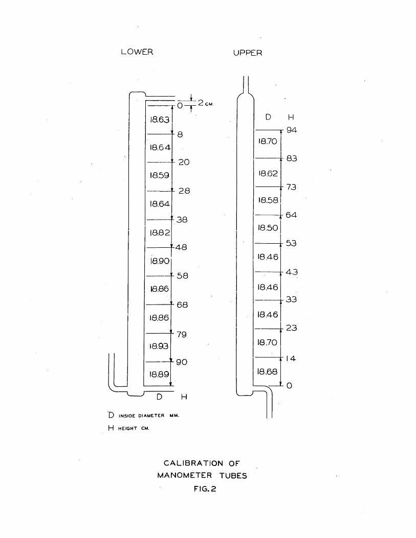
LOWER UPPER
rl5----:L----r 0T,2 CM.
18.631
---'-8
18.64
-----f- 20
18.59
---- 2818.64
--~38
18.82
-----.'48
18.90'
--'-f.- 58
18.86
---J. 68
18.86
7918.93
---~90
IS.S9
D H
'D INSIDE DIAMETER MM.
H HEIGHT CM.
I
D
18.70
18.62
18.581
~Is.501
18.46
18.46---~
18.46
~8.70 t-
H
94
S3
73
64
53
43
33
23
CALIBRATION OF
MANOMETER TUBES
FIG.2

-27
upper tube rests in a pocket in the center spacer, and thelower tube is supported similarly by the lower spacer. Thetops of the two tubes are held in place by circular steelrings surrounding the tubes with three radial set screws 600
apart around the circumference. The upper and lower tubeswere mounted directly above one another as indicated in PartI, figure (2A) so that when the two mercury menisci are viewedwith the two cathetorneter telescopes) the axes of the telescopesare in a vertical plane. The scale can then be viewed by bothtelescopes simultaneously with but a single rotation of thecathetometer bar.
The mercury column is enclosed by a housing two sides ofwhich consist of plywood board and are removable to giveaccess to the inside of the housing. The third side is ofheavier wood and is used to secure the pressure and vacuumleads. The remaining side is a panel of plate glass whichfits flush against the front flanges of the steel channelbeams which are provided with rubber gaskets and serves asa window for viewing the mercury levels.
The manometer housing forms a thermostated air bathregulated by a mercury regulator of 350 c.c. capacity~ There1s a second glass plate fitting flush against the back flangesof the steel channel beams which are also provided with rubbergaskets so that air can be circulated by means of an electricai-ly propelled fan u~ the rear of the housing and down along the

-28-
length of the column. On the inside of the rear wall of thehousing are mounted an electric resistance heater, coolingcoils and the mercury regulator. The temperature of themercury is measured by three single junction copper-constantanthermocouples evenly distributed along the length of the column.These thermocouples are immersed in cylindrica,lmercury wells.The wells are of the same diameter as the manometer tubes andare supported from the bed of one of the channel beams. Thetemperature of the mercury was regulated at some temperaturebetween 28°C. and 32°C. depending on room temperature. Atemperature gradient existed along the column caused by lossof heat from the thermostat to the surroundings through thefront glass plate as the circulating air progressed down alongthe column. Under the best conditions the temperature of thetop of the column was O.loC. higher than the bottom. Thetemperature difference at times attained a maximum value of0.4°C. These values of the gradient apply for the totallength of the column (2 meters); but since the pressures ob-served were all less than 1 atm, it is probable that theaverage temperature of the mercury in the section of thecolumn used could be determined to t O.loC. The thermostatoperated most efficiently when it was regulated only slightlyabove'room temperature. Since room temperature varied attimes several degrees e., tilethermostat was seldom operatingat its greatest efficiency. The difference in temperaturebetween the top and bottom of the room which at times alsoamounted to several degrees e. was also an unfavorable factor

-29-
in regulating the thermostat temperature •The mercury menisci are illuminated by diffuse light
sources behind the mercury surfaces and in line with the axesof the telescopes. The light sources consist of shielded 6 V.bulbs behind blue tracing cloth. Extraneous light and reflec-tion from the front halves of the menisci are eliminated bysemi-cylindrical blackened shields which fit closely aroundthe rear semi-circumferences of the manometer tubes. A slotwas cut out of the lower edge of these shields as shown inPart I, figure (2F) so that only the center portions of themenisci are visible. The light sources and shields slide ontrolleys running the length of the mercury column and can beadjusted to the desired position behind the mercury surfacesfrom outside the manometer housing by a system of pulleys.
The vacuum arm of the manometer is evacuated by meansof a mercury diffusion pump and a Hyvac fore pump. The res-idual gas pressure is measured by means of a McLeod Gauge.The gauge was calibrated by measuring the total volume of thebulb and capillary and the volume of the capillary per unitlength by weighing the contained mercury.
Total we1~h~ (nf contained Hg. at (24°0.)= 1162.185 gr.Total volume = 84.090 c.c.

-30-
Calibration of Capillary
W gr. (24°o. ) hem. dW gr. (24°0. ) d hem.~----~~~-~--------~-~------~----~---------------~~~-----~-~-73.0146 0 0 073.4735 1.7856 .4589 1.785673.9793 3.6119 .5058 1.826374.6354 6.3094 .6561 2.697575.5305 9.9212 .8951 3.611876.0854 12.1438 .5549 2.2226
w= weight of Hg + weighing bottleh= distance from closed end of the capillary.
Average cross section of capillary = .01901 cm2•
The vacuum arm of the manometer is shut off with amercury seal. Part I, figure (20) shows the arrangement ofthe McLeod gauge and seal. The vacuum arm was pumped outregularly at monthly intervals. The pressure at no time duringthese periods exceeded .001 m.m.Scale: The scale ~as a 2 meter invar bar graduated in milli-
" ""-meters, and was made by the Societ~ Genevo"ise, SWitzerland.The scale was calibrated by the U.S. Bureau of Standards inOctober, 1934. The lengths of the sub intervals of the scalespaced every 10 centimeters are given in Table IV. The cali-bration was made with the scale in a horizontal position sup-port~d at the two points indicated by the arrows on the sideof the bar.
For use in this work the Bcale is supported verticallyalong a steel H-beam. The arrangement of the mounting isshown in Plate II. The scale is hung from the upper support

-31-
TAB~E IVCalibration of the Subintervals:
Length of Subintervals at 20°C
Interval Length0 to 10 em. 100.0021 mm.0 to 20 em. 200.0036 mm.0 to 30 em. 300.0048 mm.0 to 40 em. 400.0051 mm.0 to 50 em. 500.0053 mm.0 to 60 em. 600.0055 mm.0 to 70 em. 700.0014 mm.0 to 80 em. 800.0009 mm.0 to 90 em. 899.9992 mm.0 to 100 em. 1000.0000 mm.0 to 110 em. 1099.9988 mm.0 to 120 em. 1199.9991 mm.0 to 130 em. 1299.9995 mm.0 to 140 em. 1399.9991. mm.0 to 150 em. 1499.9996 mm.0 to 160 em. 1599.9998 mm.0 to 170 em. 1699.9958 mm.0 to 1HO em. 1799.9947 mm.0 to 190 em. 1899.9940 mm.0 to 200 em. 1999.9957 mm.
The values of these lengths as given above are not in error byI
more than 0.001 mm.

-32-
which is free to rotate in perp6ndicu~ planes. The lowersupport does not carry any of the weight, but merely nervesto adjust and hold the scale in a perpendicular position.Allowance was made at the lower support for the unequal therm-al expansion of the H-beam and invar bar. The center ofgravity of scale and upper support was adjusted by counterweights in order that when these two members wer~ hangingfreely, the equilibrium position would be such that thescale hang in a perpendicular position. Then no bending mo-moment is introduced when the scale is held rigidly perpendic-ular by the lower support. The correction for the elongationof the scale caused by shifting the scale from a horizontal
(~)position to a vertical position was found by Benedict tobe negligible for a 2 meter invar scale similar to the onedescribed.
The scale is lighted by two 6 volt spot light reftectors,one mounted on each telescope carriage. The scale was rotatedat such an angle that no directly reflected light entered thetelescopes. The two lights were adjusted so that the appear-ance of the scale was the same tLl"'ougheach telescope. It wasfound tha.t the settings of the cross hair on a scale dimensionwere more" reproducible if the scales lights were adjusted sothat the scale-rulings appeared as bright lines on a darkbackground. When this condition exists, the rulings arevisible largely as a result of scattered light.
-33-
Cathetometer: The cathetometer bar is 8 feet long and 1 3/4inches in diameter. It is mounted on a vertical steel Ibeam by means of two ball bearing supports one at each endof the bar. The telescope carriages are keyed to the bar and slidefreely along the length of the shaft. The carriages can beclamped at any desired height on the shaft by means of splitcollars and set screws. The bar and telescopes can be rotatedas 8 unit around the axis of the bar.
The telescopes were tightly clamped in the carriages.On top of each telescope was mounted a floating "bubble level.The axes of these levels and the telescopes were accuratelyadjusted ~ be parallel. Leveling of the telescopes was ac-compli~hed by leveling screws on the carriages.
The eye pieces of the telescopes are of the positiveRamsden type with a magnifying power of 12.5 x. The objectiveshave a focal length of 162 m.m. The eye pieces are fittedwith stationary vertical and adJustable horizontal crosshairs. The horizontal cross hair is moved up and down ver-tically by means of a micrometer scre~. The plane of thecross hairs is between the objective anQ the eye piece ~ndcoincides with the plane of the image formed by the objectivewhen the system is properly focused. The micrometer headswere divided into 100 divisions .. Each division correspondedapproximately to .008 m.m. Tenths of a division could beestimated. The micrometer icrews were calibrated for uni-

-34-
formity by comparing the number of division corresponding toa given rn.m. interval on the scale for different sections ofthe screw. The results of this calibration appear in Table V.Adjustment of the Manometer System: The beam~ supporting themercury column, scale and cathetometer are rigidly held ateach end. The bottoms are bolted to heavy slate blocks whichare provided with leveling screws. The tops of the beams arepivoted to a false ceiling by means of universal jointswhich allow for adjustments in any horizontal direction androtation around the axis of the support. The adjustment ofa system similar to this has been taken up by Benedlct(29)who discusses in detail the adjustment of the three unitparts to perpendicularity, focusing of the system~ scaleana manometer lighting and other critical factors in pres-sure measurements.

-35-
TABL~ V
Calibration of Micrometer Screws._---for Uniformity
Upper Lower.Telescope (V2-V1) Telescope (V2..:..V1)
Scale division 10~.C 103.9 1 til.ffi. 78.7 78.8 1 m.m.vernier settings 0.0 121.6 121.6 0.3 119.3 119.35.3 126.9 121.6 5.3 124.4 119.19.8 131.2 121.4 10.1 129.4 119.3
15.0 136.5 121.5 15.3 134.5 119.219.5 111.0 121.5 20.1 139.3 119.224.6 146.2 121.6 25.1 144.3 119.230.1 151.8 121.7 30.1 149.1 119.0
35.1 156.8 121.7 35.5 154.7 119.240.5 161.9 121.4 39.7 158.8 119.144.3 165.9 121.6 45.7 164.8 119.149.5 171.1 121.6 49.9 168.9 119.0
55.1 176.7 121.6 54.8 174.0 119.260.1 181.6 121.5 60.2 179.2 119.065.8 187.3 121.5 64.9 184.1 119.270.7 191.3 121.6 70.2 189.3 119.175.2 196.8 121.6 74.9 194.0 119.179.8 101.3 121.5 79.9 199.0 119.185.8 7.3 121.5 85.1 204.3 119.290.0 11.6 121.6 90.1 209.3 119.295.2 16.8 121.6 94.7 213.8 119.1
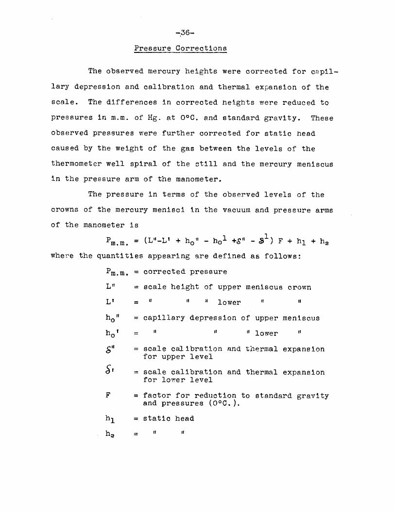
-,36-
Pressure Corrections
The observed mercury heights were corrected for capil-lary depression and calibration and thermal expansion of thescale. The differences in corrected heights were reduced topressures in m.m. of Hg. at DoC. and standard gravity. Theseobserved pressures were further corrected for static headcaused by the weight of the gas between the levels of thethermometer well spiral of the still and the mercury meniscusin the pressure arm of the manometer.
The pressure in terms of the observed levels of thecrowns of the mercury menisci in the vacuum and pressure armsof the manometer is
Pm•m• = (Llt_Ll + holt - hol +8" - Sl) F + hI + h2
where the quantities appearing are defined as follows:P =m.m. corrected pressureLit = scale height of upper meniscus crownL' = II II II lower It "ho " = capillary depression of upper meniscusho , = II " " lo\ver II
SIt = scale calibration and thermal expansionfor upper level
$. = scale calibration and thermal expansionfor IO'\1!er 1evel
F = factor for reduction to standard gravityand pressures (OoC. ).
hI = static headh2 = II II

-37-
Capillary Depression: Capillary depressions were calculated(30 )from the Lohnstein formula. The measured values of the
(31 )capillary depressions of Cawood and Patterson for tubes of(29).14 m.m. to 18 m.m. in diameter were found by Benedict to
agree ~ith the calculated values to .005 m.m. if the surfacetension of Hg. was taken as' 476 dynes/cm. The capillary depres-sion is given by
II "
" "meniscus heightradius of the tube.8 (dimensionless)
ho =h =R =J.( =
~o::: 84 --k ~. [- R ~ _2 ""'V' - --<-<.-1<2/ ]r+ Vi-~ Cl, Z t:< ;;:,
:z.t:t..zcapillary depression in m.m.
I p = density of Hg. at 25°C.a = ----_ .... -.-.-
VP~ } (J= surface tension of Hg.Za-
U = 476 dynes cm2 (Int. Critical Tables, IV, 144 )13.521 gr/cm 3 ( " " II II, 458 )P =980.397 cm./sec 2g =
The values of ho were calculated at.l m.m. intervalsfor meniscus heights from .5 m.m. to 1.9 m.m. Since thediameters of the manometer tubes were not uniform, the valueof ho depended on the position of the meniscus in the tube.The values' of ho lor each meniscus height(h) were calculatedat 10 em. intervale along the lengths of the tubes. The

co~rlrlorlmro(.0
oo~roro~~m~mm~OIDWIDOCOooOro~mmmm~N~rlrlrl~~~~~N~~~~~~~~ID~~ID~~~~~~ID~0
00
00
00
00
00
00
00
00
00
...........
..
..
...
.
oo~ooNrom~m~~~~mroco~~~~~~n~~~~~~~~IDmmrnmm~w~~~~~~~~~~ID~ID~ID~~~~0
00
00
00
00
00
00
00
00
00
........
...
.....
...
nmmm~~~OO~~Nm~rlrlW~orn~OrlrlrlN~~~~~~~~~~~~~L
()U
)~
~to
LOLO
InID
to~
~~
l!)~
LD.q
iLDlD
00
00
00
00
00
00
00
00
00
0.....
...
....
..
...
..m~~~mmo~oo~nn~nooro~~rorommromoo~~N~~~~~~OON~~~~~~~~tD~~~~tD~~tD~~tD0
00
00
00
00
00
00
00
00
00
...........
.......
.oom~~Nrloo~OOoo~~n~nmm~~ID~~w~~mmmmrororlrlrlommoc~
~~
~~
~~
~~
~~
~~
~t!)
~~
~~l
00
00
00
00
00
00
00
00
00
0....
.....
..
....
...
.~omm~~NIDoo~roIDoo~Ncom~IDnnnnn~IDIDwID~~romro~IDIDtD~~~~~~~~~~~~~~~~~~~0
00
00
00
00
00
00
00
00
00
..........
...
..
..
..ID
(\10
)m~
r0rl~rlrl
t--~
00
0~
OJ~
~oOOOOrl~~nnooN~~~~~~N..q1
"f~
~~
~~
~~
~~
~~
~~
~~
-'Qf~
00
00
00
00
00
00
00
00
00
0.......
...
.tDNmm~~m~mmW~~~~~l!)rl~C'-
~C'--
~C'-com
0())m
enmM
r-irl
r-i0
0m
nn~~~~n~~n~~~~~~~~~o~~~~~~~~~~~~~~~~~~~
....-\roco~
MW
0ID~
~M
(\1C
\200en
C\2corl
~~~~~~~C'-ID~WIDroroOOC'-~~~nn~~n~nn~nn~~~nnnnn0
00
00
00
00
00
00
00
00
00
.......
...
....
..
..
.tt:)
0~
tottJmO
J~
0000m
roC'-
r:--~
~l'-
~Icorlrlrlrlrlrln~~~Noo~~~~n~oo~
t"Jn~
ttJnt')
~t')~
~t')n
t')~to
~['£Jn
00
00
00
00
00
00
00
00
00
0.....
...
.......
....
oronno~CX)ororotD~rlrl~roooQroroC'-rorororomommmmrlrlrloommooOONOOOONNttJOONNoonnt')nnwoo0
00
00
00
00
00
00
00
00
00
.....
....
...
...
...
.w~mmWrlN~ooworo~~~rl~nro~~~~~~ID~mwm~~~~~~~~(\}
C\200C\2
\.\1NN
C\lN(\2N
00C\2N
N00
C\1N
000
00
00
00
00
00
00
00
00
00
......
...
......
..
..NO~~ooW~l>~~~C\2~~tD~ro(nN~rlrlrlrlrlN~ooNooN~n~~ooooooNOONNooNooOOooNNNNOOOOOOooNN0
00
00
00
00
00
00
00
00
00
......
...
.......
..
.coIDoororlmrlmm~~~C'-~wooow~~romC'-roromrorororommmmmenrorlrlrlrlrlrlrlrlrlrlrlrlrlrlrlrlrlrlrl0
00
00
00
00
00
00
00
00
00
......
o~oooooooooooooocooo1
00
00
00
00
00
tD
~~
~~
~~
tD
orlOO~~~w~~mO~~~~mID~ror-lrlrlrlrlrlrlrlrl
o.£1Q.Ott:G-tos::o
HoM
:>toC
/)Q)
(1)rl
s...,0
0..cj
Q)E-t
(:l
~~asrlrloM~aso
,rot"':>I

..
...
.
-
t0O~m~~~LOOOOLOrlmtOOC\2~CO~t0tOmm,...-lC\2mOONC\2t0LOLO~m~tD~m
mOOOOrlrlO,...-l,...-l,...-lrlrl,...-l,...-l,...-lrl,...-l,...-l,...-l,...-l
C\200000000000000000000
LO~tOLOrltOm~t0LO~~OOoo~~O~~m
toto
000
C\2to0
ri,...-l
toto
LOC'-
COm,...-l
::0m
Q)
C\?C\2
OOO,...-l,...-l,...-l,...-lrl,...-lrlrlrlrl,...-lrlC\2,...-lrl,...-lC\200000000000000000000
toC\2
oC\2
C\2~0
to(!)00
00l'0
(()LOt""J
~,...-l
COl'0
(!)(,()tom
~t0~oomO,...-loomooOO,...-lt0t0LOtOn~~tOo
00O,...-l,...-l
0OO,...-l,...-l,...-l,...-l,...-l,...-l,...-l,...-l,...-lrl,...-l
00000000000000000000
0~LO~mm~rlt00~mC\2~,...-lC\2rlm,...-l~t0LO~mmO~m~mmmrl,...-lt0~rlO,...-lt0OOOOO,...-lOOOOOO,...-lrlrlrl,...-lrl,...-l,...-l00000000000000000000
mrl,...-lrl,...-lO~~mLOO,...-lN~OOmLO~~~C\2LO~mmO(()tOLO~~rommO,...-lrooooooOOOOOrlOOOOOOOO,...-lrlOOO,...-l00000000000000000000
~C
Oto
t.O~
rlto
~to
0~
tot'J
\0lD
~0
LO~\0
C\2~(!)~rom~LO~tOLOwC'-~rom(!)LOLO~0000000000000000000000000000000000000000
(!)LO,...-lmLOC\2(!)LOC\2LO~mt0~t00~OOLO~C\2~(!)(!)~OO~~t0~t0~LO~~~t0C\2C\2~0000000000000000000000000000000000000000
~C\2~~m~LOt0mO,...-l~~~rl~m,...-lt0~C\2~LOW~~t0~rlt0NC\2t0t0~~OOOrl0000000000000000000000000000000000000000..
.....
.......
It0mC\2~rl~LO,...-lLOLO~m~~OOOO~.~Nt0~t0LOlDtOtOC\2C\20rlOO,...-l,...-lrlrl,...-l~t0,...-l0000000000000000000000000000000000000000..
.....
..,-
..
..
II
II
I,...-lWOOrlt0LO~mro0C\2mLOm~C\2Nt00t0C\2t0~LOLOLO,...-lOOOrlOOOOO~LO(!)~0000000000000000000000000000000000000000
.....
....
......
JI
II
1I
II
1I
0000000000000000000000000000000000000000,...-IC\2t0~LO(!)~COmO,...-l~t0~LO(!)~OOmO
rl,...-lrl,...-lrl,...-l,...-l,...-l,...-lr-fC\2
Q)
rltU()
{1)Ha:s>s::H«Hot:o..-l.p(
)H
Q)H
H>
~oQ)
o,...-l..0
CDm
~8
::s.pCO~Q)
P4SQ)
8rdt:tUs::o..-l.pa1H..0..-l,...-la1o
ImtoI
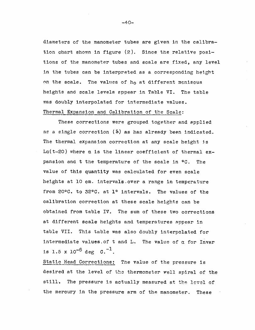
-40-
diameters of the manometer tubes are given in the calibra-tion chart shown in figure (2). Since the relative posi-tions of the manometer tubes and scale are fixed, any levelin the tubes can be interpreted as a corresponding heighton the scale. The values of ho at different meniscusheights and scale levels appear in Table VI. The tablewas doubly interpolated for intermediate values.Thermal Expansion and Ca~ibration of the Scale:
These corrections were grouped together and 8ppliedae a single correction (~) as has already been indicated.The thermal expansion correction at any scale height jsLa(t-20) where a is the linear coefficient of thermal ex-pansion and t the temperature of the scale in °C. Thevalue of this quantity was calculated for even scaleheights at 10 cm. intervals.over a range in temperaturefrom 20°C. to 32°C. at 1° intervals. The values of thecalibration correction at these scale heights can beobtained from table IV. The sum of these two correctionsat different scale heights and temperatures Rppear intable VII. This table was also doubly interpolated forintermediate values.of t and L. The value of a for Invar
6 -1is 1.5 x 10- deg C. .Static Head Corrections: The value. of the pressure isdesired at the level of the thermometer well spiral of thestill. The pressure is actually measured at the level ofthe mercury in the pressure arm of the manometer. These

-41-
two pressures differ by the pressure head caused by the weightof the gas included between tbece two levels.
The total static head correction is the sum of twoparts hl and h2. The first part (hU is the pressure head be-tween the levels of the mercury in the pressure arm and of thevapor, gas interface in the still condenser. The second part(h~ is the pressure head of the vapor between this interfaceand the thermometer well spiral.
The level of the vapor gas interface was assumed toremain constant and was measured to be 13 ern. above the thermom-eter well spiral. Hence hI varied with the pressure in thesystem, the height of pressure arm and room temperature. Roomtemperature was assumed to be constant at 25°; and since thepressure depended only on the pressure arm height, the valueof hI could be expressed in terms of this height alone. Thevapor, gas interface was at a scale level of 63 em. When themercury in the pressure arm was at this level the value of hIbecame O. The value of hI was calculated from the followingequation
hI (m.m. Hg) =d x Pm.m.13.53 x 760
13.53 gr/cm3 = density of Hg. at 25°C.d = of gas in m~nometer system.at
25°C. and 760 m.m.P.m.mT pressure in the system.
d (He) =-.000164
d( Na) = .001148

-42-
The values of hI at even heights of the pressure arm appear
in Table VIII.
Table VIIIStatic Head Correction (hI)
Short Armneight
He N2 condo at -80°C.
0 m.m. -.0201 m.m. -.1405 m.m. -.1223 m.m.50 -.0176 -.1229 -.1056
100 -.0153 -.1064 -.0900150 -.0130 -.0910 -.0755200 -.0110 -.0767 -.0621250 -.0091 -.0636 -.0499300 -.0074 -.0515 -.0388350 -.0058 -.0405 -.0287400 -.0044 -.0308 -.0199450 -.0031 -.0220 -.0120500 -.0021 -.0145 -.0047550 -.0012 -.0080 .0002600 -.0004 -.0027 .0046650 .0002 .0016 .0076700 .0007 .0047 .0100750 .0010 .0067 .0112800 .0011 .0076 .0112850 .0010 .0073 .0100900 .0010 .0071 .0089950 .0005 .0035 .0044
The second part of the correction (ha) varied with
the pressure, temperature in the still and the composition of
the vapor. The values of ha ~cre calculated from the expressiond1 x 298 x 1 x Pm.m.
h2 (m.m. of Hg) = --------------------760 Y 13.53 x (t+273)
dl = density of the vapor at 25°C. and 760 m.m.t = temperature in the still.
p m.m. = pressure 1n the system.
1 == 130 m.m.

-43-
The densities of mixtures of chloroform and ethanolvapors were taken as a linear function of the composition .
dl = .004895 - .003007 Ywhere y is the mole fraction of ethanol in the vapor.
dl (water vapor) = .000738 gr./cm3
3dl (alcohol vapor) = .001888 gr./cmdl (chloroform vapor) = .004895 grm./cm3
h2
= ~:~~~_~_~l_~_~m~~~ __(t + 273)
Reduct ion to Pressures at OOC. and Sta.ndardGravity: These twocorrections both appear as multiplying factors applied to thed1.fference in corrected mercury levels. The product of thetwo factors are combined and are represented by F. The factorfor the reduction to pressures at OOC. is the ratio of thedensity of mercury at OOC. to the density at the temperatureof the manometer mercury. The gravity correction enters as aconstant factor and is equal to thA ratio of the value ofstandard gravity to the value of gravity at the location wherepressures are measured. The values of F have been calculated
(29 )by Benedict over a range in temperature from 20°C. to 32°C.at 0.1° intervals, and were later revised by KaminSky(8) andBaisdell(9). These values of F appear in Table IX. Values at.010C. intervals were obtained by interpolation. The calcnla-tion of this table was based on the value of gravity of

-44-
2980,400 em/see in room 6-231 of this laboratory and the valueof standard gravity of 980.86c cm/sec2. The pressure measure-ments in this work were carried out in room 6-232. An error of+- 0.1°0. in the temperature of the manometer mercury produces
+an error of approximately .01 m.m. in the reduced pressureat a pressure of 1 meter.

---ooaCrlo.E.So.p
><HCDr-I,0tUE-t
cor-I
a
...
~~
CJto
toIf)
r-1l.'0tOlO
l'I),.,If..to
toO
')(J)(j)
mm
m...
...
....
JLf)
l'

-46-
Procedure for Measuring the Pressure
The manometer light sources were adjusted behindthe mercury levels. The cathetometer bar was rotated untilthe vertical cross hairs of the upper and lower telescopeswere in the center of the upper and lower minisci. Each tel-escope was adjusted vertically until the crown of the meniscusw~s at the center of the field of view. The shields were loweredbehind the mercury surfaces until the distance between the crownof the menisci and the lower edges of the shields appeared inthe telescopes to be about 1 m.m. This distance was accurate-ly reproducible by the aid of a vertical scale in the plane ofthe cross hairs which appeared directly beside the image of themeniscus in the field of view. The telescopes had two parallelhorizontal cross hairs which appeared to be about 1 m.m. apart.The upper cross hair was used as a reference line and the lowerone as an additional aid in adjusting the heights of the shields.
The upper horizontal cross hair of each telescope wasfirst set on the line of intersection of the mercury meniscusand wall of the manometer tube. This level was detected byshining a light on the manometer tube opposite the mercury sur-face. The cross hair was set at the point where light ceased tobe reflected from the cylindrical mercury surface. This levelwas assumed to be the bottom of meniscus. The value of thislevel was read to .01 m.m. but was uncertain to .05m.m. Themicrometer head was then rotated noting the number of complete

-47-
revolutions of the screw, until the cross hair was set on thecrown of the meniscus. Three separate settings were made on thecrown of the upper and lower mercury menisci. The three separatesettings usually agreed within .002 m.m. and seldom deviatedmore than .004 m.m. The manometer lights should be switched offimmediately after finishing observations on the mercury surfacesin order to prevent unnecessary fluctuations in the manometerthermostat as B result of the heat generated by the light fila-ments.
When the levels of the crowns and bottoms of both theupper and lower menisci had been observed, the cathetometer barwas rotated until the vertical cross hairs were in the center ofthe scale. The micrometer head of each telescope was rotated un-til the reference cross hair coincided with the next lowest m.m .
.scale dimension. Three separate settings were made at thislevel, and the values usually agreed within .002 m.m. Themicrometer head was thenrotated until the reference cross hairhad traveled down the scale.l m.m. and coincided with'the nextlo~est m.~. scale division. Three separate settings were madeat this level. This procedure gave the number of divisions ofthe micrometer head of each telescope per m.m., and served tocheck the screw calibration at various pos1tlons on the scale.
The temperature of the scale was measured by amercury thermometer graduated in O.loC. intervals suspendedbeside the scale at about its midpoint. The temperature ofthe manometer mercury was determined by measuring the E.M.F.

-4t3-
Table X
vernier reading vernier readinglower telescope upper telescope
bottom of 62.4 16.6(1)
meniscus
Crown of 60.1 85.8meniscus 60.4 85.9
60.2 85.9
scale 30.5 45.0setting 30.5 845 m.m. 45.1 1153 m.m.
30.4 44.9
calibration 11.2(1) 23.9(1)
setting 11.1 844 m.m. 24.0 1152 m.m.11.2 24.0
Scale Temperature = 27.2 E.M.F of thermo junctionslower .001125 voltscenter .001127 II
upper .001129 "

-49-
of the three thermo junctions in the manometer housing.An example of the manner of recording readings taken
for a pressure measurement appea~s in Table X. The superscript (1) added to a mlcrnmeter head setting indicates a ro-tation of more than one complete revolution of the screw. Thecorr"ected pressure was calculated in the following manner.Lower mercury level.screw calibration =130.5 - 11.2 = 119.3 divisions/m.m.
160.2 - 62.4meniscus height = ------------- = .e3 m.m.
119.3
60.2 - 30.5L = 84a-+ ~--------- = 845.24e m.m.119.3
Upper mercury level.
divisionsscrew calibration = 145.0 - 24.0 = 121.0 --------------
m.m.
121.085.9-45.0
meniscus height = 185.9 - 16.6,....- ....-.------.-..~ = 1.40 m.m.
L" = 1153 + ---------- = 1153.338 m.m.121.0
L"-Lr = 1153.338 - 845.248 = 307.990 m.rn •
• , f
P = (307. 990+ho" - ho I + S - Sm.m.
At this point the analysis of the dlstillate gave a

-50-
value of y = .8838 The mean mercury temperature of the man-ometer mercury for this pressure was taken as the average ofcenter and lower thermo junction temperatures.
S I :: .009 /I
ho' :: .031 m.m.
Avera~e E.M.F = .0011264= 32.00x2.3860xlO (.001126-.001291)II tOO.
" It
ho " = .049 m.m.S /I = .011 II
hI :: .007 "h2 = .008 "
F = .9946579corrected Pm.m. = 306.379 ID.m.
It was necessary to measure pressures below 160 m.m.with only one telescope. The construction of the telescopecarriages prevent the axes of the two telescopes from beingmoved closer together. In this procedure alternate readingswere taken on the tipper and lower menisci by sliding thetelescope up and down on the bar. It was necessary.to levelthe telescope before each meniscus and scale reading. Thepressures measured in this manner had an uncertainty of .05m.m. caused mainly be error in leveling of the telesqope.Mechanical imperfections in the bearings of the cathetometerbar may also be a source of error in this procedure.

-51-
Materials
The distillations necessary in the purifications ofboth ethanol and chloroform were carried out in a vacuumjacketed Vigreux fractionating column with controlled reflux.The toiler and receiver of the still had a capacity of 2 liters.The parts of the still were entirely of glass and were as-sembled by means of ground glass joints. The vent communicat-ing with the atmosphere passed through a caloium chloridedrying tube. Heat was furnished by means of an electricallyheated air bath surrounding the still boiler." The rate ofdistillation was controlled by a variable resistance in serieswith the heater.Ethanol: Commercial absolute alcohol was purified in 2 literquantities. Purified iodine crystals (1 gr./liter) ~ere addedto the alcohol and the mixture allowed to stand for 24 hours.The mixture was introduced into the still end after refluxingfor 2 hours was allowed to distil at the rate of 150 c.c. perhour. The first and last quarters of this distillation wererejected. The middle fract~on was refluxed over zinc woolfor about 12 hours to remove the iodine that came over duringthe first distillation. After being certaln of the removal ofall the dissolved iodine as indicated by the disappearance ofthe yellow. color, the alcohol was allowed to distil at therate of 75 c.c. per hour; and the middle third collected.

-52-
The pure alcohol was immediately transferred to 100 c.c. stop-pered glass bottles.Chloroform: Chloroform ~ac also purified in 2 liter quantities.It was first refluxed for 12 hours over phosphoric anhydrideand then allowed to distil at ab0ut 150 c.c. per hour. Thefirst a~d last quarters were rejected. The middle fractionwas redistilled over anhydrous codium carbonate at a rate of75 c.c. per hour, and the fir~t and last thirds rejected.These distillations were carried out in the dark. The nec-essary measurements on pure chloroform were made as quicklyas possible after the purification process. About 1% byvolume of ethanol was added to pure chloroform that was tobe stored and the mixture transferred to 100 c.c. glass stop-pered bottles. This mixture of chloroform and ethanol wasstored in the da.rk.

-E.3-
Density Measurements
A diagram of the pycnometers used is shown infigure (3). Two similar pycnometers were used, one for analy-sis of the distlllate sample and the other for the liquidsample. The bulbs had a volume of approximately 11.5 c.c.The capillaries had a bore of .6 ID.m. Each capillary wasprovided with a fine file scratch (A) which served as areference level. On the tops of the capillaries weremounted short lengths of glass tubing which were sealed by
means of ground glass stoppers. Ample space was allowedbetween the stoppers and the mouths of the capillarieb totake care of any expansion of the liquid that might occur.
Density measurements and the pyconorneter calibrationswere carried out at 25°C. A small thermostated water bathwas used to maintain this temperature. The temperature ofthe bath was measured by a Beckmann thermometer which wasset by comparison with platinum resistance thermometer #103.The temperature of the thermostat during a density Measure-
+ment was constant at 25.00 - .01°0.Before each density determination the pycnometers
were thoroughly dried by placing them in an evacuated belljar for about 1/2 hour. They were then weighed after theyhad been dipped in water and dried with a damp cloth. Theliquid wa~ introduced into the pycnometers through the sidearm capillary from a 25 c.c. pipette. After filling thestoppered pycnometers were suspended in the thermostat for

-A--
PYCNOMETER.
FIG.3

-54-
10 minutes. At the end of this period the level of theliquid in the capillaries was adjusted to the reference marksby removing the excess liquid with filter paper. The filledvessels were then removed from the bath, dryed with a dampcloth and weighed. It was found that better weighings couldbe obtained if the vessels were wiped with a slightly damprather than a dry cloth. The static charge induced on thesurface by wiping with a damp cloth is probably smaller thanthat induced with a dry one.
A glass tare of size and shape comparable to eachof the pycnorneters was used on the weight pan of the balanceas a counter poise. This tare was subject to the same treat-ment as the pycnometers. The 10s8 of weight of the vesselsresulting from evaporation of the liquid through the groundglass joints was negligible during the time required forweighing.
The two pycnometers we~e designated by the symbols. PI and Pa" PI had a single file scratch on both capillaries
while P2 had two scratches on the center capillary.. In P2 theupper of these two scratches was used as a reference level.Weighings were made by suspending the pycn~meters from thepan support of the balance by means of a loop of copper wire.The different weights to be considered then combine as fol-lows:

-55-
Wp (empty) + W (wire) = W (tare) + WI (weights)
~~-~~~::~--~_~_~__:_~_:_~_~_~__~_~_:~_~__: 2W(liquid) = (W"-W.) weights (in air)
These weights of the liquid in air were reduced toweight in vacuum by correcting for the buoyancy effect as a
result of the air displaced by the liquid and brass weights.The values of (W"-WI) were sufficiently large to justify neglect-ing the buoyancy effect of the fr~ctional gram weights. The
3density of brass WaR taken as 8.0 gr./cm .The largest difference observed between observed
values of Wp (empty) was .5 m. gr. The values of W (liquid)for pure liquids could be checked to within 1 m. gr.
The two pycnometers were ~ibrated by determing theweight of water contained at 25.0°0. The calibration valuesare given below.
Wp = 11.43921 volume 11.43921 11.4'1313 c.c.gr. PI = -----.------ =.997044
volume P2 11.29631= ....---------
.99'1044= 11.32980 II
On Jan. £, 1937 it was necessary to repai~ a smallcrack which developed in the side wall of P2. PI and Pa wereboth recalibrated at this time. It was found that P2 hadchanged its volume slightly but PI had not. The values forthe reca11brations of Pa ~re given below.
volume P2 11.28828= -------- ....- =•.99704411.32175 e.e.

All density measurements made later than Jan. 6, 1937are based on this value of the volume of Pa.
Thp.accuracy of the analysis of chloroform, ethanolmixtures as carried out in this work appears to be limited byerrors arising from changes in composition resulting fromevaporation while handling the mixtures rather than by theerror in the actual density measurements.

-57-BIBLIOGRAPHY
(1) J.W. Gibbe, Collected Works, Vol. IDuhem, Ann. de l'Eoole norma1e eye., 3 it 9 (1887)
(2) E.H.J. Cuneaus, Zeit, ,Phys. Chern. 36, 232 (1901).(3) J.v. Zawldski, Zeit. Phys. Chem., 35, 129 (1900).(4) M.A. Rosanoff, A.B. Lamb, F.E. Breithut, J.A.C.S.,
31, 448 (1909).(5) J. Sameshima, J.A.C.S., 40, 1482 (1918).(6) J. Sameshima, Journ. Fac. of Soience of Tokyo, (1)
!, 63 (1925).(7) T.H. Chilton, Proceedings of Fourth Symp. of Chem.
Eng. Education, 04, (1935).(8) J. Kaminsky, Doctor's Thesis (V), (1937).(9) B.E. Blaisdell, Doetor's Thesis (V), (1936).(10) L.B. Smith, F.G. Keyes, H.J. Gerry, Pro. of the
Am. Aced. 69, 137 (1934).(11) H. Hirobe, Journ. Fac. of Science of Tokyo, (1)
1, 155 (1925).(12) Castille and Henri, Bull. Soc. Chim. BioI., ~, 299
(1924).(13) L. Harris, J.A.C.S., 55, 1940 (1933).(14) U.S. Industrial Sales Co., ~altlmoreJMd.(15) J. Timmerman, F. Martin, Jour. Chim. Phys., ~J
763 (1926).(16) G. Rutledge, Phys. Rev., 40, 262 (1932).(17) J.J. Coleman, F.E.E. Germann, J. Chern. Phys., !,
847 (1933).

~, 1803 (1914 ).D.F. Othmer, Ind. Eng. Chern., 20, 743 (1928).C.P. Smyth, E.W. Engel, J.A.C.S., 51, 2646 (1929).
-58-
Bibliography Continued
(18) M.E. DuC1aux, Ann. de Chim. et de Phys. XIV (5),305 (1878)
(19) M.A. Rosanoff, C.W. Easley, J.A.C.S., 31, 953 (1909).(20) M.A. Rosanoff, C.W. Bacon, R.H. White, J •.A.C.S.,
(21 )(22)
(23) F. Hovorka and D. Dreisbach, J.A.C.S , 66, IG64 (1934)(24) W. Sweitoslawski, Bull. Acad. Scl. Polonaise, 434 (1929).(25) W.H. Julius., Annalen der Physik (Wiedeman), 56, 151
(1895) .(26) S.S. Prentiss, Doctor1s Thesis (V),(1930).(27) M.O. Benedict, Doctor1s Thesis (V), (1935).(28) J.A. Beattie, B.E. Blaisdell, J. Kaminsky, Pro. of
the Am. Acad., 71, 375 (1937).(29) M. Benedict, Doctor's Thesis (V)(1936) .(30) T. Lohnstein, Ann. der Physik, 33, 296 (1910).(31) W. Cawood, H.S. Patterson, Trans. Farad. Soc.,
XXIX, 514 (1933).(32) J.Q. Cope, W.K. Lewis, H.C. Weber, Ind.Eng.Chem.,
23, 88? (1931).(33) R.H. Newton, Ind.Eng.Chem., 27, 302, (1935).(34) R.R. Newton, B.F. Dodge, Ind.Eng.Chem.,27, 577,(1935).(35) F.G. Keys, L.B. Smith, H.J. Gerry, Pro. of the Am.
Acad. 70, 319, (1936).

Part IFigure
(1)(2 )
(3)
(4 )
(5 )
(6 )
(7)
(8 )
(9 )
(10)(11)
-59-
List of Figures
FollowsTitle
Page
Equilibrium Still 4Manometer System 9
Deviation Ourve-Specific Volume andOomposition 14
P-x-y isotherms, 35°0.,45°0.,55°0. 23P-Py-P(l-y) at 45°0. 24
A log P-y isotherms, 35°0.,45°0.,55°0. 26
(x-y) obs., rR(x-y) and 33-y(l-y) -~_!~-~- y at 3500.,4500.5500.dy~lE (ethanol) - x at 35°0.,45°0.,55°0. 38~2E (chloroform)-x at 35°C.,450C.,550C. 38
EFx -x 38
E E EHXJ-TSX ,Fx - x at 45°0. 41
Part II(1) Deviation curve for calibration
of 20 junction thermocoupleCalibration of Manometer TubesPycnometer
22
26
53
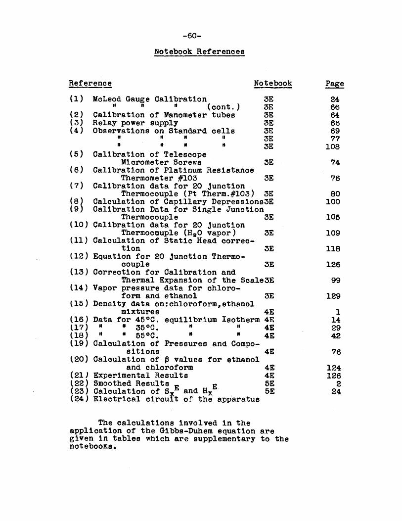
-60-Notebook Referenoes
Referenoe
Calibration of TelesoopeMicrometer Screws 3E
Calibration of Platinum ResistanceThermometer 1103 3E
Calibration data for 20 junotionThermocouple (Pt Therm.#I03) 3E
Calculation of Capillary Depressions3ECalibration Data for Single Junotion
Thermocouple 3ECalibration data for 20 junction
Thermocouple (HaO vapor) 3ECalculation of Statio Head correo-
tion 3EEquation for 20 Junotion Thermo-
couple 3ECorreotion for Calibration and
Thermal Expansion of the Scale3EVapor pressure data for chloro-
form and ethanol 3EDensity data on:chloroform,ethanol
mixtures 4EData for 45°C. equilibrium Isotherm 4E
n 1350C. .. .. 41It at 550C. • .. 4E
Calculation of Pressures and Compo-sitions 4E
Calculation of ~ values for ethanoland chloroform 4E
Experimental Results 4ESmoothed Results E 5ECalculation of S E and Hx - 5EEleotrical circuIt of the apparatus
(1)
(2)(3)(4 )
(5)
(6)
(7)
(8)(9)
(10 )
(11)
{12)
(13 )
(14)(15 )
(16 )(17)(18)(19)(20)
(21 )(22)(23)(24 )
MoLeod Gauge Calibration" " n (cont.)
Calibration of UBnometer tubesRelay power supplyObservations on Standard cells
" .... nn If. It
Notebook3E3E3E3E3E3E3E
Page246664666977
10874
7680
100105109118
126
99129
1142942
76
124126
224
The oalculations involved in theapplication of the Gibbs-DUhem equation aregiven in tables Which are supplementary to thenoteboo.1ts.

-61-Biographical Sketoh
Charles L. Raymond was born on May 18, 1911 inSchenectadY, New YorK. He attended Howe Grammar Sohoolthrough the seventh grade and transferred at the begin-ning of the eighth grade to Central Park IntermediateSohool. He graduated from this school in June 1925after having completed work through the first year ofhigh sohool. He attended Nott Terrace High School forthree years and graduated in the Scientifio oourse inJune 1928. He entered Union College in September 1928anddurlng a four year period pursued the course ofstudy prescribed by the Chemistry Course. He graduatedin June 1932 with a degree of B.S. in Ohemistry. Hewas elected an associate member of Sigma Xi, and wasaffiliated with the Phi Gamma Delta Fraternity. Hereturned to Union College for a year's graduate workand received the degree of M.S. in Chemistry in June1933. The results of the work included in the Thesispresented for the degree appear 1n the Journal ofPhysical Chemistry, ~, 663 (1934). He was admittedto the Graduate Sohool of the Mass. lnst. of Tech. 1nSeptember 1934 and has since been pursuing a course ot
study leading to a degree of Ph.D. in Physical Chemistry.He was elected to membership 1n Sigma Xi in May 1936.