1

Contents NUMERICAL ARRAYS ................................................................................................................................... 1

1-Dimensional Arrays .............................................................................................................................. 2

Entering array values over multiple lines – MATLAB’s line continuation ............................................ 5

2-Dimensional Arrays .............................................................................................................................. 5

Arithmetic with Arrays ............................................................................................................................. 7

Entering Numerical Arrays with the input() Command ................................................................... 10

Arrays and Built-in Functions................................................................................................................. 10

Combining Arrays .................................................................................................................................. 10

Transpose Operator ............................................................................................................................... 11

Shortcuts for Defining and Manipulating Arrays ................................................................................... 12

The colon operator ............................................................................................................................. 12

The end command ............................................................................................................................ 15

The size() and numel() commands ........................................................................................... 15

CHARACTER ARRAYS ................................................................................................................................. 17

NUMERICAL ARRAYS MATLAB is designed for handling matrices (arrays). You can think of arrays as a collection of boxes that contain similar items (each element of the array is one box). We use arrays when we want to store a lot of similar data in a single variable. A scalar variable, which stores the value of just a single number, is simply a 1x1 array – it has only one element and that element is the numerical value that is stored in the variable. This is a special type of array and in general arrays will have many elements to store multiple values. For example, if we want to use MATLAB to find the mean and standard deviation of 100 students’ test scores, we first need to store all the scores in memory. It would be quite lengthy and complicated to make a new variable for each test score. Instead, we can store all of the scores in a single variable – this variable will be an array, and each element of the array will store one test score.

Although in theory arrays can have many dimensions, we usually only deal with 1D arrays (vectors) or 2D arrays (matrices) in MAE10.

For 2D arrays, the dimensions/size of the array is expressed as #ROWS x #COLUMNS. A 1D array is a 2D array with only one row or only one column. Here are some visualizations of various size arrays:

2

1x6:

3x1:

4x2:

An array is composed of elements. A 1x6 array is 1-dimensional; it has 1 row, 6 columns, and has 6 elements total. A 3x1 array is 1-dimensional; it has 3 rows, 1 column, and has 3 elements total. A 4x2 array is 2-dimensional; it has 4 rows, 2 columns, and has 8 elements total. Extending this concept into 3+ dimensions, a 4x2x3 array is 3-dimensional and has 24 elements and a 2x10x3x2 array is 4-

dimensional and has 120 elements. 1-Dimensional Arrays

First, we will discuss 1D arrays since they are simpler to understand than 2D arrays. Every time you

create a variable with a single value, you create a 1D array that is 1x1 in size. A 1x1 array is typically referred to as a scalar, meaning that it is just a single value.

>> a = 52.4

a =

52.4000

>> whos

Name Size Bytes Class Attributes

a 1x1 8 double

3

The variable a is a 1x1 array. Let’s create a bigger array. You can define arrays by enclosing multiple separate numbers in brackets. Each individual element in the array is separated by a comma, a space, or both.

>> cat = [0.1 , 0.2, 0.4]

cat =

0.1000 0.2000 0.4000

>> dog = [1.1 1.2 2.4]

dog =

1.1000 1.2000 2.4000

>> whos

Name Size Bytes Class Attributes

cat 1x3 24 double

dog 1x3 24 double

We have created two 1x3 arrays that contain double precision data (e.g., floating point numbers). Here are graphical illustrations of the cat and dog arrays. You refer to a particular element in the array by putting the element number in parenthesis following the array name. 0.1 0.2 0.4

cat(1)cat(2)cat(3)

1.1 1.2 2.4

dog(1)dog(2)dog(3)

>> cat(3)

ans =

0.4000

>> dog(1)

ans =

1.1000

4

>> dog(4)

Index exceeds matrix dimensions.

Notice that we get an error message if we try to access a non-existent array element.

Once created, you can use elements of an array to do mathematical operations or anything else that you would do with a scalar variable.

>> dog(1) + cat(2)

ans =

1.3000

>> rat = cat(1)^2

rat =

0.0100

You can also change the individual values stored in an array. In this case you will replace (overwrite) the old value in the position that you give (by the element #) with a new value that you specify (whatever is to the right hand side of the equals sign).

>> dog(1) = 5

dog =

5.0000 1.2000 2.4000

>> dog(2) = dog(3)

dog =

5.0000 2.4000 2.4000

Notice that in the above examples we are changing only one element of the array at a time and the other remain unchanged. Although all the values are contained within the same array, each element can be accessed or changed independently from the others. We can also add additional elements to arrays very easily in MATLAB. However, note that in many other programming languages (such as FORTRAN), this is not allowed – you would need to declare the size of your array ahead of time. In MATLAB, we simply specify the array name and element number to the left hand side of the equals sign, and provide the value to the right hand side of the equals sign.

5

>> dog(4) = 10

dog =

5.0000 2.4000 2.4000 10.0000

>> whos

Name Size Bytes Class Attributes

ans 1x1 8 double

cat 1x3 24 double

dog 1x4 32 double

rat 1x1 8 double The array dog is now a 1x4 array. Note that we did not change any other values stored in the array when we added a new element. Entering array values over multiple lines – MATLAB’s line continuation

If you want to define a long 1D array and do not have enough room to easily fit all the values on one line, you can use an ellipsis (…) to continue inputting values on the next line. The ellipsis essentially tells MATLAB to treat the next line as part of the previous line that is terminated with an ellipsis.

>> turtle = [1 3 5 6 3 5 3.3 ...

55 66 77 888]

turtle =

Columns 1 through 6

1.0000 3.0000 5.0000 6.0000 3.0000 5.0000

Columns 7 through 11

3.3000 55.0000 66.0000 77.0000 888.0000

The line continuation command does not apply only to arrays. It can be used anywhere in MATLAB to split a command over multiple lines. 2-Dimensional Arrays 2D arrays are very similar to 1D arrays, except you now need to worry about both rows and columns.

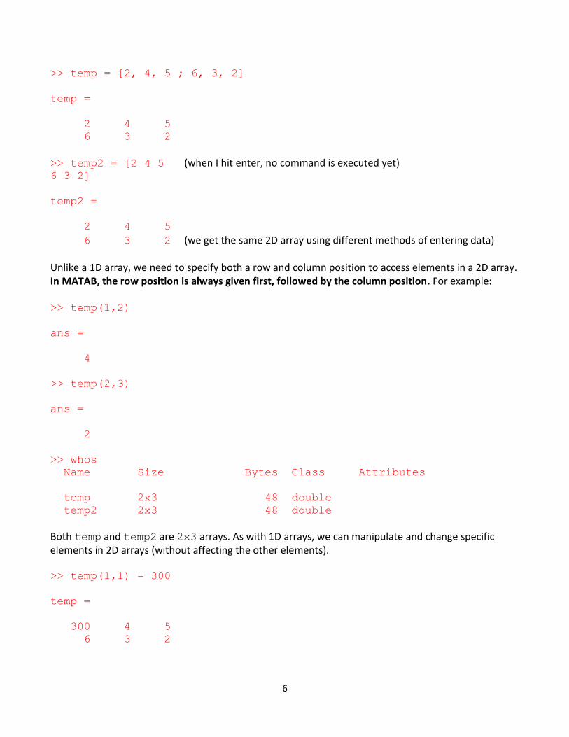
You separate rows by using a semicolon (;) or by hitting the return key (starting a new line) and inputting values over multiple lines.

6

>> temp = [2, 4, 5 ; 6, 3, 2]

temp =

2 4 5

6 3 2

>> temp2 = [2 4 5 (when I hit enter, no command is executed yet) 6 3 2]

temp2 =

2 4 5

6 3 2 (we get the same 2D array using different methods of entering data) Unlike a 1D array, we need to specify both a row and column position to access elements in a 2D array. In MATAB, the row position is always given first, followed by the column position. For example: >> temp(1,2)

ans =

4

>> temp(2,3)

ans =

2

>> whos

Name Size Bytes Class Attributes

temp 2x3 48 double

temp2 2x3 48 double

Both temp and temp2 are 2x3 arrays. As with 1D arrays, we can manipulate and change specific elements in 2D arrays (without affecting the other elements).

>> temp(1,1) = 300

temp =

300 4 5

6 3 2

7

>> temp(2,2) = temp(1,1) + 1

temp =

300 4 5

6 301 2

>> a = temp(2,2) + temp(2,3)

a =

303

Arithmetic with Arrays

There will be times where you will want to perform an operation on all the elements of an array. For example, multiply all the elements of an array by a constant (a scalar). >> a = [2, 3, 9 ; 4, 4, 7] (a is a 2x3 array) a =

2 3 9

4 4 7

>> d = 3

d =

3

>> b = d.*a

b =

6 9 27

12 12 21

Notice we used the .* operator instead of just the * operator. Adding a period in front of the arithmetic operator means “apply this operation to every element of the array.” When we only are multiplying, dividing, adding, or subtracting an array by a scalar (1x1 array), the dot operator is not necessary. In fact, using the dot operator with addition or subtraction between a scalar and an array will produce an error. This is because arithmetic operations between a scalar and an array automatically apply the scalar value to all elements of the array. The dot operator is only necessary for element-wise multiplication and division between two arrays, where both arrays are larger than 1x1 (e.g., have 2 or more elements).

8

Let’s look at some examples to illustrate these points. >> b2 = d*a (We get the same result using .* and * in this case since d is a scalar) b2 =

6 9 27

12 12 21

>> a = a + 1

a =

3 4 10

5 5 8

>> a = a .+ 1

a = a .+ 1

↑

Error: Unexpected MATLAB operator.

>> a = a/10

a =

0.3000 0.4000 1.0000

0.5000 0.5000 0.8000

The real use for the dot operator comes when we are doing multiplication or division between two arrays, where both arrays are larger than 1x1. >> a

a =

0.3000 0.4000 1.0000

0.5000 0.5000 0.8000

>> b

b =

6 9 27

12 12 21

9

>> c = a*b

Error using *

Inner matrix dimensions must agree.

>> c = a.*b

c =

1.8000 3.6000 27.0000

6.0000 6.0000 16.8000

You can see that in the first attempt to create c, we got an error. This is because MATLAB interpreted this as traditional matrix multiplication (as in linear algebra). Using the .* operation tells MATLAB to do element-wise multiplication. That is, multiply every element of a by every corresponding element

of b. Note that in this case, a and b must be the same size. The same rules apply if we try to raise the array a to the power of 2:

>> a^2

Error using ^

Inputs must be a scalar and a square matrix.

To compute elementwise POWER, use POWER (.^) instead.

>> a.^2

ans =

0.0900 0.1600 1.0000

0.2500 0.2500 0.6400

This is because MATLAB is trying to multiply the array a by itself to complete the exponentiation

operation (a 2x3 array multiplied by another 2x3 array), which is forbidden by the rules of traditional matrix multiplication learned in linear algebra. If you want to square each element of the array a, use .^ as we did above. You can see that MATLAB even gave you this as a hint. To summarize, here are some key points for the dot operator:

Use the dot operator (a period) before multiplication or division between two arrays when you want to apply the operation to every corresponding element of the two arrays.

o Do not use the dot operator for addition or subtraction between two arrays. Addition and subtraction automatically operate element-wise between to arrays and between a scalar and an array. Doing so will result in an error as we saw above.

o Any two arrays must be the same size in order to perform any element-wise operation between them.

10

The dot operator is never required when doing arithmetic between a scalar and an array. The operation automatically applies the scalar element-wise to every element of the array.

Entering Numerical Arrays with the input() Command When using the input() command, you can enter multiple values simultaneously and store them in a single array by putting brackets around two or more numbers separate by commas and/or spaces. >> val = input('Enter some values:')

Enter some values:[2 5, 7]

val =

2 5 7

However, keep in mind that this requires knowledge of MATLAB syntax (i.e., you must use brackets when entering multiple values to be stored in a single array) and in practice the user of your code may not be familiar with MATLAB. Thus, it is safer to have the user enter the values one at a time. When asking for multiple values, a loop can be utilized so that the user enters values one at a time and the array automatically is constructed element by element. This method is discussed later in the context of for and while loops. Arrays and Built-in Functions If you use an array as an argument for a built-in function, the function will automatically act element-wise on all individual elements in the array. For example: >> d = sqrt(val)

d =

1.4142 2.2361 2.6458

Note: Not all built-in functions behave in this manner. Certain functions operate on the columns of arrays, rather than on each individual element. Examples are provided later that illustrate this point.

Combining Arrays You can combine multiple arrays into a single array. The new array will be of larger size than the two individual arrays and its dimensions (#rows and #cols) are determined by how you combine the arrays (e.g., by adding along the same row, by adding a new row, etc.).

11

>> time = [0, 4, 8, 12];

>> temps = [55, 52, 58, 63];

>> array1 = [time ; temps]

array1 =

0 4 8 12

55 52 58 63

>> whos

Name Size Bytes Class Attributes

array1 2x4 64 double

d 1x3 24 double

temps 1x4 32 double

time 1x4 32 double

val 1x3 24 double

Transpose Operator If you want to change your array from a MxN array to a NxM, you can use the transpose operator. The transpose operator is invoked by using the full transpose() command, or by placing a single quotation mark after the array variable name. There are many times when this operator is useful, including when you want to view data in a more convenient format. Transposing an array essentially switches its rows and columns. Mathematically, AT(i,j) = A(j,i) >> time = [0, 4, 8, 12];

>> temps = [55, 52, 58, 63];

>> array1 = [time ; temps]

array1 = (This style doesn’t look that great)

0 4 8 12

55 52 58 63

>> transpose(array1)

ans =

0 55

4 52

8 58

12 63

12

>> array1' (This style looks much better)

ans =

0 55

4 52

8 58

12 63

There are other ways to do this operation using loops (if such a built-in function is not available), which you will learn later. Shortcuts for Defining and Manipulating Arrays MATLAB is great for dealing with arrays. It should come as no surprise that there are a lot of nifty commands that will save you a lot of time when manipulating data in arrays. We will not be using all these shortcuts in this course because many are not available in most other programming languages. However, it is important that you know how they work and how to use them effectively. The colon operator In general, this operator is used in the following manner to create arrays: a : c : b Which essentially means “from a to b in steps of c” – a is the initial value, b is the final value, and c is the step size.

For example, 0 : 0.25 : 2 means go from 0 to 2 in steps of 0.25

If you omit c, the default value of c, the step size, is 1 0 : 2 means go from 0 to 2 in steps of 1 Note that the extra spaces between the values and the colon itself are not necessary – extra blank spaces are ignored by MATLAB but are commonly used to improve readability.

When using the colon operator by itself (meaning just : with no a, b, or c) the colon operator means “everything.” This is discussed in more detail in the indexing arrays section below.

Creating arrays with evenly spaced values If you want to make an array with element values that are evenly spaced, you can use the colon operator in the following way.

13

>> time = [0:0.25:1.25]

time =

0 0.2500 0.5000 0.7500 1.0000 1.2500

The colon operator can be used with negative numbers, decimals/fractions, variables that have already been defined (and are in memory), and so on. For example: >> x = -10

x =

-10

>> y = 5

y =

5

>> my_array = x:y:10

my_array =

-10 -5 0 5 10

There are a few important things to remember when using the colon operator to go from an initial value to a final value. When using the colon operator, MATLAB will never “overshoot” (go past) the final value, and MATLAB will never “break” the step size (not take a full step). >> var1 = 0:3:10

var1 =

0 3 6 9

Here, we tried to create an array starting at 0 and ending at 10 using a step size of 3. Beginning at the initial value, we starting adding elements using our step size. However, after 9, we cannot go to 12 because this would mean going past the final value, and we cannot go to 10 because that would mean not taking a full step. Thus, MATLAB stops at 9. The following is another example using a step size that is both negative and not an integer:

14

>> var2 = 10:-(1/3):8.5

var2 =

10.0000 9.6667 9.3333 9.0000 8.6667

Here, our step size is -1/3, but we cannot reach 8.5 exactly, so we “stop early” at the nearest full step that can be taken. It is very important that you remember these rules for the colon operator as they will apply in exactly the same fashion when we learn for loops. Indexing arrays with the colon operator You also can use the colon operator by itself to extract part of an array. In this case, the colon operator means “everything” (e.g., all rows, all columns, or both, depending on where you put it). For example, let’s create a 3x3 array and extract the second column out of the 3x3 array.

>> a = [3.5 4.6 7.1 ; 1.1 -0.9 -1. ; 3.3 3.3 2.3]

a =

3.5000 4.6000 7.1000

1.1000 -0.9000 -1.0000

3.3000 3.3000 2.3000

>> b = a(:,2) (all rows, second column only) b =

4.6000

-0.9000

3.3000

Here, the colon operator alone means “all rows” (since it is in the row position) and since we have a 2 in the column position, the output (saved into b) is all rows in the 2nd column of a. If the colon operator is used in an array index and appears between two numbers, it means extract from the first number to the second number. For example, >> c = a(2:3, 2:3) (extract rows 2 to 3, columns 2 to 3 from a and put them into c) c =

-0.9000 -1.0000

3.3000 2.3000

15

CAUTION: When using the colon operator to index a range of values in an array, the initial value, final value, and step size MUST all be integers. This is because array indices must be positive integers. Using decimals, negative numbers, etc., will result in an error. The end command If you forget the number of rows or columns in your array, you can use the end command, which is a keyword in MATLAB to signify the final element in an array. Remember when indexing arrays with more than one dimension, we need to give both a row and column index. The end command can be used in either or both as shown below. >> A = [1 3 5 7 9]

A =

1 3 5 7 9

>> B = [1 2 3; 4 5 6]

B =

1 2 3

4 5 6

>> A(end)

ans =

9

>> B(end,end)

ans =

6

The end command can only be used when indexing an array to signify the final row/column position. It cannot be used anywhere else in MATLAB. The size() and numel() commands If you want to know how many elements are in an array, use the numel() command.

If you want to know the number of elements in each dimension, use the size() command.

16

>> a = [2:2:10 ; 3:3:15]

a =

2 4 6 8 10

3 6 9 12 15

>> numel(a)

ans =

10

>> size(a)

ans =

2 5 (The size() command returns the number of rows and columns) In general, you want to store the number of rows and columns in variables so that you can use them to index your array later in your code (this is essential when using loops later in the course). >> [rows,cols] = size(a)

rows =

2

cols =

5

>> Num_Elements = rows*cols

Num_Elements =

10

Note that we had to use two variables to the left-hand side of the equals since (in brackets) since the size() command has two outputs. This is different than most other built-in functions that have only one output. The names of these variables does not matter (they do not need to be named rows and cols).

17

CHARACTER ARRAYS Earlier we touched upon character data. Character data is perfect for arrays – each individual character of a word or phrase can be stored in an array element. Note that every character takes one element of the array, whether that character is a letter, a space, an underscore, a period, and so on. >> food = 'cheese'

food =

cheese

>> drink = 'pepsi'

drink =

pepsi

You can visualize these arrays as a series of boxes as before:

food: c h e e s e

drink: p e p s I

Character arrays are indexed and manipulated in the same way as numerical arrays.

>> food(1) (we can get just the first element of the array food)

ans =

c

>> drink(5)

ans =

i

>> var23 = food(1:3) (we can get a some but not all of the array’s elements)

var23 =

che

18

>> whos

Name Size Bytes Class Attributes

ans 1x1 2 char

drink 1x5 10 char

food 1x6 12 char

var23 1x3 6 char

You can combine character string arrays into a single array to make one long character string. This is done in the same way as combining numerical arrays. >> a = 'hi'

a =

hi

>> b = 'bye'

b =

bye

>> c = [a,b]

c =

hibye

>> d = [a ' ' b]

d =

hi bye

We combined character strings in the past when using the disp() command. In that case, we converted a numerical value into a string using the num2str() command, then combined the two

strings in a single disp() command (note the use of brackets, which signifies an array). In myfile.m: x = 5;

disp(['The value of x is ' , num2str(x)])

Sample output: The value of x is 5

19

Arrays are at the heart of all numerical computations. Arrays are the means by which we can easily store large amounts of data in variables. Regardless of what programming language you are using, understanding how to create, manipulate, index, and do arithmetic with arrays is essential. Furthermore, MATLAB is designed specifically to be very efficient at handling arrays and has countless built in functions to easily solve equations that involve arrays. There are many other types of arrays that can be used in MATLAB such as logical arrays or cell arrays, but they are beyond the scope of MAE10. However, it is very important that you understand how to work with numerical and character arrays as they will be recurring throughout the course.