the virtues of hesitation: optimal timing in a non

American Economic Review 2015, 105(3): 1147–1176 http://dx.doi.org/10.1257/aer.20121282

1147

The Virtues of Hesitation: Optimal Timing in a Non-Stationary World †

By Urmee Khan and Maxwell B. Stinchcombe *

In many economic, political, and social situations, circumstances change at random points in time, reacting is costly, and reactions appropriate to present circumstances may become inappropriate upon future changes, requiring further costly reaction. Waiting is informative if arrival of the next change has non-constant hazard rate. We identify two classes of situations: in the first, delayed reaction is optimal only when the hazard rate of further changes is decreasing; in the second, it is optimal only when the hazard rate of further changes is increasing. These results in semi-Markovian decision theory provide motivations for building delay into decision systems. (JEL C61, D72, D82, D83, K10, M11)

In many social, economic, and political situations, there is a stochastic environ-ment that changes at random points in time and responding to these changes entails significant costs. Given that a new state may give way to yet another, potentially making today’s optimal action again obsolete, and given that actions are costly, the question is whether to respond to a change in the environment or to delay.

Variants of this problem have been extensively analyzed in economics (for exam-ple Boyarchenko and Levendorskiı̆ 2007, Stokey 2009, and the references therein). However, a crucial aspect of most existing analyses is that the passage of time by itself does not reveal any information. By contrast, we study problems in which the passage of time without a change contains information about the arrival time of the next change, problems in which there may be value to delaying decisions beyond the usual option value of waiting.1 We begin with examples where the length of time that a change has survived may be of crucial importance to its future longevity.

1 See McGuire and Kable (2012, 2013) for experimental evidence on how hazard rate patterns affect delay of gratification behavior.

* Khan: Department of Economics, University of California, Riverside, Sproul 3131, 900 University Avenue, Riverside, CA 92506 (e-mail: [email protected]); Stinchcombe: Department of Economics, University of Texas at Austin, BRB 2.102A, 1 University Station, Austin, TX 78712 (e-mail: [email protected]). Many thanks to Martin Dumav, Zahid Arefin Chowdhury, Takashi Hayashi, Marcin Peski, Gordan Zitkovic, and Mihai Sirbu for their much appreciated help, to seminar participants at UC Riverside, Delhi School of Economics, and University of Bielefeld and conference participants at the IHS Summer Research Conference (2010), Midwest Political Science Association Conference (2010), Midwest Theory Conference (2011), GAMES (2012), and SSCW (2012) for helpful comments and discussions. We are grateful to three anonymous referees for detailed and highly insightful feedback that has helped us improve the paper. All remaining errors are ours. The first author gratefully acknowledges the financial support of a Summer Research Fellowship from the Institute of Humane Studies. The authors declare that they have no relevant or material financial interests that relate to the research described in this paper.

† Go to http://dx.doi.org/10.1257/aer.20121282 to visit the article page for additional materials and author disclosure statement(s).

http://dx.doi.org/10.1257/aer.20121282

mailto:[email protected]

mailto:[email protected]

http://dx.doi.org/10.1257/aer.20121282

1148 THE AMERICAN ECONOMIC REVIEW MARCH 2015

I. Optimal Timing in the Face of Non-Stationarity

A. Political Change

Political processes in a democratic system are driven by “political issues” and the configuration of opinions and attitudes of the polity on these issues. Such configu-rations are hardly, if ever, static. There are slow and gradual changes that take place side by side with rapid and explosive changes. Some changes are long-lasting, some short-lived. As Carmines and Stimson (1990, p. 5) say:

… we shall see that issues, like species, can evolve to fit new niches as old ones disappear. But, unless they evolve to new forms, all issues are temporary. Most vanish at their birth. Some have the same duration as the wars, recessions, and scandals that created them. Some become highly associated with other similar issues or with the party system and thereby lose their independent impact. And some last so long as to reconstruct the political system that produced them … .

The Vietnam War and the Watergate scandal seem to have very little traces left today either in public attitude or legislative response to the issues of war and exec-utive power respectively, but they were the biggest issues of their day. On the other hand, the Civil Rights Movement and its aftermath marked a fundamental realign-ment in US politics. In general, some ideas and opinions “wear out their welcome” after a time, perhaps through changes in the conditions that gave rise to them, per-haps by the accumulation of counterarguments to their veracity. Hence, the likeli-hood that such an idea would become irrelevant increases with time. By contrast, some types of issues or opinions tend to get more entrenched the longer they live. Political actors in various capacities try to cope and make decisions in the face of such “issue evolution” (Carmines and Stimson 1990). Legislatures choose whether or not to change a law, supreme courts decide whether or not to reinterpret or over-turn past precedents, political parties decide whether or not to realign politically and redefine the agenda. Oftentimes, the most crucial ingredient in such decisions is the aspect of timing.

Each of these decisions entails some fixed cost either to the society at large or the actor herself.2 One would have to trade off the immediate gains with substantial future losses if the initial change that triggered the costly action turns out to be rel-atively short-lived.

Another class of political decisions have to do with effective but costly response to a possibly impending crisis. Again, timing is of the essence, but in a very different way. When it appears that a costly prevention or crisis-averting action might need to be taken, the crux of an executive decision then becomes how to delay the cost as much as possible, without being too late to actually prevent, or at least lower the likelihood or the cost of, the crisis. Impending wars, international conflicts, painful and unpopular reforms, or a system overhaul, all of these are examples.

2 In case of legislative changes and court decisions, the citizens have to readjust and reoptimize with respect to the new rules. In case of a political party, realignment may mean losing a traditional support base and adjusting to a new one.

1149Khan and Stinchcombe: the VirtueS of heSitationVoL. 105 no. 3

The following two subsections discuss examples drawn from arenas of political decision making where the need for deliberation and caution interplay with the need for quick and decisive action, and one of the challenges of institution design turns out to be the demarcation of the different spheres where in one should be empha-sized at the expense of the other.

Constitutional Amendments.—Constitutions establish the fundamental legal structures of a society. They are meta-institutions through which institutions are introduced, reformed, and interpreted (Ostrom 1990). A constitution and the legal order it creates must have the support of, or at least tacit approval of, the governed to have legitimacy. Maintaining the legitimacy and relevance of a constitution requires a certain degree of adaptability or flexibility to change because technology, environ-ment and public opinion are forever changing. On the other hand, the basic value of a constitution lies in its stability because it coordinates the actions and expectations of people and reduces the uncertainty in the environment (Hardin 2003). Hence the basic trade-off between “commitment” and “flexibility” lies at the heart of the con-stitution design problem, as encapsulated in the famous exchange between Thomas Jefferson and James Madison in Smith (1995).3 It is also costly to change the con-stitution because it acts as a coordination device for peoples’ behavior, and changes are likely to impose large adjustment costs on significant parts of the population and disrupt ancillary institutions that grow around the constitution (Hardin 2003).

From these perspectives, it is reasonable to presume that an optimal rule for con-stitutional change should be more sensitive to long-lasting changes than to transitory changes. It is clear that waiting longer will help answer whether a change will have a longer or shorter total life, but what matters for decisions is the longer or shorter future life of the change. One trade-off is between costly unneeded or ultimately unwanted changes (e.g., Prohibition) and undermining the legitimacy of the consti-tutional regime by ignoring new realities. It is from this perspective that we study the general question of why some changes in laws should be more difficult to imple-ment, and what this should depend on.

Under study is a class of explanations that we regard as complementary to the many previously offered ones, a class of explanations based on the observation that the persistence of changes in sentiment have predictive power for the future length of time the changes will last. For us the question becomes “How much longer should one wait before acting?” The dynamically consistent answer depends both on the costliness of the action and the costliness of its reversal.

The US Constitution has had four different amendments that have extended vot-ing rights to different parts of the population: Amendment XV (1870), which was passed at the end of the Civil War, extended suffrage to men independent of race or previous condition of servitude; XIX (1920) extended suffrage to women; XXIV (1964) made poll taxes illegal; and XXVI (1971) extended suffrage to those 18 years of age or older. These formalized long-lived widely-shared changes in senti-ment, but Amendment XVIII (1919), Prohibition, was an expensive and short-lived

3 For interesting empirical evidence to the effect that flexibility actually helps the sustainability of constitutions, see Elkins, Ginsburg, and Melton (2009), for an analysis of the ways in which flexibility must be structured for the functioning and survival of formal systems that must adjust to changing circumstances, see Stinchcombe (2001).


failure, being repealed 14 years later by Amendment XXI (1933) (Amar 2006 is a detailed history of the amendments to the US Constitution).

If one dates the beginning of the women’s suffrage movement to the 1848 Seneca Falls Convention, it took 72 years for Amendment XIX to pass.4 At various points in the political process, there was evidence that the recognition of women’s rights to vote would be long-lasting: the passage of suffrage at the state level in west-ern states by the early twentieth century;5 the nation’s westward expansion and the Civil War leading to an expanded need for women both in industrial settings and as teachers; the gradual increase in the numbers of college educated and professional women; and unionization movements among female professions in the late 1800s and early 1900s. Even after one could perhaps clearly see that general sentiment had shifted in favor of the Nineteenth Amendment, there was (much) further delay in implementing what turns out to have been a long-lasting change in sentiment. This is perhaps consistent with unwillingness to believe that so drastic a change could be long-lasting, but our analysis suggests that the relatively high cost of depriving a class of people of liberties, once granted, exaggerates the effects of such doubts.

By contrast, Prohibition proved to be very costly to society, and was short-lived, repealed 14 years later.6 The Temperance Movement had as long a history as the women’s suffrage movement, and was used by some women’s suffrage organizers as an occasion to teach women the necessity of having a voice in politics in order to achieve changes (Flexner and Fitzpatrick 1996). The implementation of Prohibition very quickly gave rise to a host of social problems accompanied by a marked increase in crimes associated with illegal selling and consumption of alcohol. Public opinion quickly turned against it. From our point of view, this was a change of action that led to a change in the distribution of the time until general sentiment was reversed.

Executive Power.—The US Constitution has a separation of powers between the executive and the legislative branches. While an extensive discussion of the virtues of such an approach, as opposed to one in which the two branches coincide, as in the United Kingdom, is outside our purview, one aspect of this separation is relevant to our motivating question here. Congress is the deliberative body, and congres-sional procedures are markedly more inclined toward caution and restraint against hasty decisions, in comparison with the structure of executive power, which enables and empowers the president to act in a quick and decisive fashion if need arises. Our observation is that it is one way to institutionally demarcate between decision problems where built-in delay could be desirable (making legislative actions more attuned to longer lasting changes), and those where not being too-late-to-be-of-any-good is the real concern (executive decisions, where delay, if at all, should come only out of prudence, not structural limitations).

4 Flexner and Fitzpatrick (1996) make an argument for an earlier date for the beginning of the movement, emphasizing the experience of female abolitionists and agitators for women’s education in the early 1800s as the roots of the suffrage movement.

5 By 1915, Arizona, California, Colorado, Idaho, Illinois, Kansas, Montana, Nevada, Oregon, Utah, Washington, and Wyoming had granted full women’s suffrage, and several other states or municipalities had granted suffrage in primary elections.

6 Prohibition was repealed by Amendment XXI, the only amendment passed by state ratifying conventions rather than by the votes of state legislatures, sparing the legislators from re-election campaigns against a dedicated cadre of single-issue voters.


We now turn to other settings in which our general methodology could be fruit-fully applied.

B. Marketing Strategy

Research in consumer behavior has shown that when and how consumers switch brands depend on the last purchased brand and time since the last purchase. The inter-purchase time may exhibit increasing or decreasing hazard rates depending on consumer characteristics like “inertia” or “variety seeking tastes” (Chintagunta 1998). It has been suggested that optimal timing of targeting consumers for mar-keting should depend on such considerations instead of the traditional demographic variables (Gönül and Ter Hofstede 2006 gives an empirical approach to optimal timing for catalog mailing). The class of optimization models under study here are directly applicable to such situations.

C. Labor Search

One of the issues relating to long-term unemployment is depletion of human capital, which might make a candidate less and less attractive to the potential employ-ers as the duration of unemployment gets longer and longer. This factor would have important implications for standard labor search models, as the value of the future discounted wage and thus the reservation wage for a job seeker would be affected. Ortego-Marti (2014) uses this insight to explain observed wage dispersion in the labor market. Also, the possibility that a long period of unsuccessful job search is taken, by potential employers, as an indication that there is something undesirable with the person, would mean a decreasing rate of arrival of a job of any given quality. This is independent of decay of human capital, and pushes the acceptance thresh-old downward. One of the key ingredients of the standard Diamond, Mortensen, Pissarides (DMP) model is a stochastic description of labor turnover, along with a model of labor-market tightness, and a bargaining model of wage determination (see Diamond 2011; Mortensen 2011; Pissarides 2011; Hall 2012 and the references therein). Our model results would be relevant for an attempt to capture non-station-arities in the first component. Recent empirical work based on the DMP model (e.g., Shimer 2005) highlights various aspects of the wage determination phenomenon that are not well explained by the stationary DMP models so far. It would be interesting to introduce non-stationarities in the job-arrival process and work out the implications. Our framework provides a minimal way of attempting that.

D. Currency Unions, International Treaties

The benefits of joining currency unions or international treaties are variable over time and leaving a currency union or abrogating a treaty is a costly decision. These two factors combine to provide the context for countries trying to devise strategies for entry, exit, and crisis management. The recent crisis in the European Monetary Union (EMU) has rekindled the discussion around the impacts of countries exiting currency unions. Opinion is sharply divided, although the majority opinion seems to be that breaking up of the Euro would be disastrous (Eichengreen 2010). On


the other hand, historically, there have been regular instances of countries leaving currency unions (Rose 2007). From the design perspective, one of the interesting features of the EMU is that there are no exit clauses. Omission of a well-defined exit clause, at the least, significantly raises the procedural cost of exiting the union, and thus can be seen as a mechanism to avoid hasty reaction by individual countries that could potentially threaten all the other members as a group. Overall, the European currency crisis and the responses to it by various parties highlight the importance of the main facets of our model: the trade-off between reacting quickly and flexibly on one hand, and the need to avoid precipitating a fast-moving crisis by unnecessarily hasty actions on the other.

E. Outline of the Paper

Section II contains three simple examples that give a sense of what is involved in the more general analyses that follow. The essential aspects of the model include: a starting state and action, i 0 and a 0 ; random times Y k+1 at which the state changes from I k to I k+1 according to a partly controlled, embedded Markov process; and the option to engage in costly changes in actions during the inter-arrival stochastic intervals, that is, between Y k and Y k+1 .

The within-interval maximization problems will be central to the dynamic anal-ysis. The first two examples in the section concern problems with only one interval, how long to search and how long to delay precautionary measures. With the intu-itions about how the optimality conditions work for a single interval in place, the last example demonstrates how the value functions for an entire dynamic problem interact with the maximization problems within intervals.

The general model, existence of optima, their recursive characterization through the value function, and the first order conditions (Euler equations) for a leading class of problems are in Section III. Section IV applies both the recursive characterization and the Euler equations to a number of problems and discusses their implications in the context of our examples. Section V concludes.

II. Three Examples

Three non-stationary problems demonstrate the essential features of the optimiza-tion problems under study and of their solutions: the optimal delay before abandon-ing search involves searching until the hazard rate for search success is low enough and falling; the optimal hesitation before implementing expensive precautionary measures involves waiting until the hazard rate is high enough and increasing; and optimal adaptations to changing circumstances involves solving a sequence of prob-lems much like the first two. We use the first two examples in analogy with the two classes of decision problems that we described in our discussion of political change.

We assume throughout that waiting times, W , have continuous densities, f , on (0, ∞) , and, possibly, an atom at ∞ . If W has an atom at ∞ , it is called an incom-plete distribution, corresponding, e.g., in search problems, to the object of search not existing or not being findable. Associated with W is the cdf, F(t) = ∫ 0

t f(x) dx , with lim t↑∞ F(t) < 1 for incomplete distributions, and the hazard rate, h(t) : = f (t) _____

1 − F(t) .


The first and second order conditions (FOCs and SOCs) have common features: the net benefits to delaying from t to t + dt take the form (a + b · h(t)) dt ; solving the FOCs requires h( t 1 ∗ ) = −a / b ; this in turn requires that a and b have opposite signs. When a is negative, the costs of delay are certain and the benefits stochastic, when a is positive, this is reversed, there is a sure benefit to delay and a stochastic cost. Further, as the net benefits must be positive before t 1 ∗ and negative afterwards, the SOCs require h ′ ( t 1 ∗ ) < 0 if a < 0 and b > 0 , and h ′ ( t 1 ∗ ) > 0 if a > 0 and b < 0 .

A. Hesitating to Cut Off Search

At a flow cost of c ≥ 0 , one can keep searching for a source of higher profits (a low cost source of a crucial input, a process breakthrough, a new product). If found, expected net flow profits of _ π result. If one abandons the search, the decision is, by assumption, irreversible, and the known alternative yields expected net flow profits of π _ , with _ π > π _ > 0 .

The non-stationary choice problem is “At what time, t 1 , does one stop searching and accept the lower π _ ?” The results we give here are special cases of Theorem 2 (below), but we give an intuitive development here.

FOCs.—The net benefits of waiting an extra instant dt at a pre- W time t 1 are (a + b ⋅ h( t 1 )) dt where: a = −(c + π _ ) incorporates the flow cost, c , and π _ is the forgone flow value of the known alternative; and delay gives a probability h( t 1 ) dt of moving the flow payoffs upward, which is worth, in present value terms, b = 1 _ r (

_ π − π _ ) . At an interior optimum, 0 < t 1 ∗ < ∞ , the FOCs are therefore h( t 1 ∗ ) = r(c + π _ ) / ( _ π − π _ ) .

SOCs.—In order for the solution just given to be a local maximum rather than a local minimum, the net benefits of waiting, 1 _ r (

_ π − π _ ) ⋅ h( t 1 ) − (c + π _ ) , must be positive for t 1 < t 1 ∗ and negative for t > t 1 ∗ . As ( _ π − π _ ) > 0 , for this to be true, the hazard rate must be decreasing at t 1 ∗ , h′( t 1 ∗ ) < 0 .

Comparative Statics.—Because the hazard rate is decreasing, the optimal t 1 ∗ is: higher for higher _ π , it is worth searching longer when the reward is larger; lower for higher c , one searches less if searching is more costly; lower for higher r , one searches less if one is more impatient; lower for higher π _ , one searches less when the fallback option is better; and higher for uniform upward shifts in h(·) , one searches more if search is more productive.7

B. Hesitating to Inoculate

Present utility flows are _ u > 0 . At issue is the optimal timing of a costly inoc-ulation or precautionary measure: an evacuation before a hurricane landfall; or a politically painful reform of a banking system before the next financial crisis. If the

7 One can also arrive at the FOCs and SOCs by explicitly writing the integrals giving the expected payoffs and differentiating. Details of the calculations for all three models in this section can be found in the online Appendix.


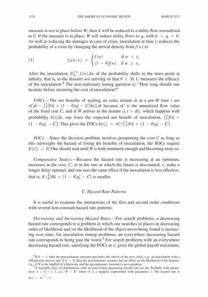
measure is not in place before W , then _ u will be reduced to a utility flow normalized to 0 . If the measure is in place, W will reduce utility flows to u _ , with _ u > u _ > 0 . As well as reducing the damages in case of crisis, inoculation at time t 1 reduces the probability of a crisis by changing the arrival density from f(w) to

(1) f θ (w; t 1 ) = { f (w) if w < t 1 (1 − θ)f(w) if w ≥ t 1 .

After the inoculation, θ ∫ t 1 ∞ f (w) dw of the probability shifts to the mass point at

infinity, that is, to the disaster not arriving so that θ ∈ [0, 1] measures the efficacy of the inoculation.8 The non-stationary timing question is, “How long should one hesitate before incurring the cost of inoculation?”

FOCs.—The net benefits of waiting an extra instant dt at a pre- W time t are rCdt − ( 1 _ r [θ

_ u + (1 − θ) u _ ] − C ) h(t) dt because rC is the annuitized flow value of the fixed cost C , and if W arrives in the instant (t, t + dt) , which happens with probability h(t) dt , one loses the expected net benefit of inoculation, ( 1 _ r [θ

_ u + (1 − θ) u _ ] − C ) . This gives the FOCs h( t 1 ∗ ) = rC / ( 1 _ r [θ

_ u + (1 − θ) u _ ] − C ) .

SOCs.—Since the decision problem involves postponing the cost C as long as this outweighs the hazard of losing the benefits of inoculation, the SOCs require h′( t 1 ∗ ) > 0 . One should wait until W is both imminent enough and becoming more so.

Comparative Statics.—Because the hazard rate is increasing at an optimum, increases in the cost, C , or in the rate at which the future is discounted, r , make a longer delay optimal, and one sees the same effect if the inoculation is less effective,

that is, if ( 1 __ r [θ _ u + (1 − θ) u _ ] − C) is smaller.

C. Hazard Rate Patterns

It is useful to examine the interactions of the first and second order conditions with several non-constant hazard rate patterns.

Decreasing and Increasing Hazard Rates.—For search problems, a decreasing hazard rate corresponds to a problem in which one searches in places in decreasing order of likelihood and/or the likelihood of the object never being found is increas-ing over time; for inoculation timing problems, an everywhere decreasing hazard rate corresponds to being past the worst.9 For search problems with an everywhere decreasing hazard rate, satisfying the FOCs at t 1 ∗ gives the global payoff maximum,

8 If θ = 1 , then the precautionary measure precludes the arrival of the next crisis, e.g., an inoculation with a 100 percent success rate. If θ = 0 , then the precautionary measure has no effect on the likelihood of the disaster, e.g., if W is the landfall of a hurricane and the precautionary measure is an evacuation.

9 A tractable class of distributions with an everywhere decreasing hazard rate are the Weibulls with param-eters λ > 0, γ > 1 , i.e., W = X γ where X is a negative exponential with parameter λ . The hazard rate is

h(t) = λ t 1−γ ____ γ / γ .


and conditional on having already searched until any T ≥ t 1 ∗ , it is optimal to stop immediately. By contrast, for inoculation problems with an everywhere decreasing hazard rate, satisfying the FOCs gives the global payoff minimum, the optimum is either at t 1 ∗ = 0 , immediate inoculation, or t 1 ∗ = ∞ , never inoculating. Further, if immediate inoculation is optimal, then conditional on not having inoculated yet, immediate inoculation is optimal until the time T ◦ > 0 at which one is indifferent between inoculating now and never inoculating.

These patterns are reversed for everywhere increasing hazard rates (e.g., Weibulls with parameters λ > 0 and 0 < γ < 1 ). For inoculation problems, satisfying the FOCs at t 1 ∗ gives the global payoff maximum and if inoculation has been delayed to any T ≥ t 1 ∗ , it is optimal to inoculate immediately. For search problems, satisfying the FOCs at t 1 ∗ gives the global payoff minimum, the optimum is either at t 1 ∗ = 0 or at t 1 ∗ = ∞ , if at t 1 ∗ = 0 , then immediate abandonment of search is optimal until the time T ◦ > 0 at which one is indifferent between abandoning search and continuing to search forever.

Some Mixed Cases.—In quality control, one often sees a “bathtub shaped” hazard rate pattern: early failures are due to manufacturing flaws and tail off; late failures are due to systems wearing out, and their hazard increases over time.10 For search problems, a bathtub hazard rate pattern corresponds to a search process that first checks the likely and easy to check locations, and if the object is not found, then the remaining locations, however unlikely or difficult to check, must be where the object is located. If the first order conditions are first met at t 1 ′ at which the hazard rate is decreasing, then t 1 ′ is a local maximum. If the FOCs are not satisfied at a later time, then t 1 ′ must also be the global maximum. If the FOCs are satisfied at a (necessarily single) later time, this is a local minimum, and t 1 ′ must be compared to t 1 = ∞ —early abandonment of search may be optimal, or unbounded search may be optimal.

For search problems, a “hump-shaped” hazard rate pattern corresponds to a search process that needs time to begin to function well, but once the likely and/or easy-to-search locations have been exhausted, it becomes clearer and clearer that the object was not there in the first place. If the first order conditions are met while the hazard rate is increasing, this is a local minimum, so either t 1 ∗ = 0 is optimal or some later time will be optimal. If a later time, t 1 ′ , corresponds to satisfying the FOCs a second (and necessarily last) time, then t 1 ′ is a local maximum, and if any search is optimal, it has a limited duration.

For inoculation problems, the hump-shaped hazard rate pattern corresponds to facing a gathering storm that may, or may not, yield a disaster, but if one is lucky enough to get through the most hazardous times without a disaster, the storm passes and the likelihood diminishes. If the first order conditions are met at a t 1 ′ where the hazard rate is increasing, then t 1 ′ is the locally optimal trade-off between delay of expensive preparations and imminent danger. Further, the next time the FOCs are satisfied will be a local minimum so that either t 1 ∗ = t 1 ′ or t 1 ∗ = ∞ is optimal—evacuate if the danger is imminent enough, otherwise try to ride it out and hope for the best.

10 This is often used as a quality control screen—overload elements for long enough that the first kinds of fail-ures are weeded out (e.g., Rausand and Høyland 2004, Ch. 2).


D. Optimal Adaptation to Changeable Circumstances

We now study a simple model of the optimal timing of adaptations to a stochastic dynamic state. Solving the entire problem involves solving a sequence of single interval problems.

States and Actions.—The first ingredients in the model are a state space, S = {i, j} , an action space, A = {a, b} , and a set of flow utilities to be discounted and inte-grated: for the “matched” state action pairs (i, a) and ( j, b) , we set u(i, a) = 1 and u( j, b) = 2 ; for the “mismatched” pairs, we set u(i, b) = u( j, a) = 0 .

Change Costs.—In our general model, change-of-action costs depend on the present action, the action one changes to in the set of available actions, and the present state. For the present model, there are four such costs. For simplicity here, we assume one can switch from a to b or back in either state, and all four switching costs are equal to C > 0 .

Change Times.—The states will change at random times. It is the costs of switch-ing actions that may make instantaneous adjustment of the action to the state subop-timal—if another change in the state is expected soon, it may not be worth incurring the cost to enjoy the extra flow. The non-stationary timing question is, “How long to hesitate before reacting?”

The state change times are random variables Y k , k = 0, 1, … with Y 0 ≡ 0 , Y k ∈ (0, ∞] for k ≥ 1 , and P( Y k < Y k+1 ) = 1 if Y k < ∞ . With I k denot-ing the state of the system for the k th state change time, starting state is i 0 , and the future states I k , k ≥ 1 . The waiting time for the k th change is defined as W k : = Y k − Y k−1 , and P( W k = ∞) > 0 corresponds to the k th waiting time having an incomplete distribution and there being a positive probability that there is never a transition away from the state I k−1 . A policy is semi-stationary if it depends only on the initial state-action pair and the within-interval time, and we will see that such policies are optimal. For any such policy, the random sequence ( i 0 , W 1 ), ( I 1 , W 2 ), … is a Markov process taking values in S × (0, ∞] that “ends” at the first k , if any, at which W k = ∞ .

In the general model, the distribution of each W k will depend on the state-action pair that is in effect at the start of each interval and the time path of action changes that occur within the interval. In this simpler version of the model, the distribution of the W k depends only on the state-action pair, (i, a) , that prevails at Y k−1 , and the time, Y k−1 + t 1 , t 1 ∈ [0, ∞] , at which the action is first changed. Because at most one change of action can be optimal and there is only one possible action to change to, a plan for an interval, denoted 𝔭 , can be specified by a single change time, t 1 ∈ [0, ∞] . Further, the stochastic structure can be summarized in a class of possibly incomplete probability density functions (pdfs) on (0, ∞) , f i 0 , a 0 ( ⋅ ; t 1 ), t 1 ∈ [0,∞] , ( i 0 , a 0 ) ∈ S × A . Because changes of actions at t 1 can affect the future but not the past, we assume that for all s ≤ t 1 < t 1 ′ ≤ ∞ and all ( i 0 , a 0 ) , f i 0 , a 0 (s; t 1 ) = f i 0 , a 0 (s; t 1 ′ ) . To put it another way, the single pdf f i 0 , a 0 ( ⋅ ; ∞) governs arrival the time of the state change up until a change of action, but the distribution of what hap-pens after that change of action can depend on the time at which it occurred.


Expected Utility.—All random variables are defined on a probability space (Ω, , P) . A stochastic interval is a subset of Ω × [0, ∞) of the form [ [ Y k , Y k+1 [ [ = [ [ Y k , Y k + W k [ [ := {(ω, t) : Y k (ω) ≤ t < Y k+1 (ω)} . If the inter-val starts with the action being a k , we specify a plan to change from a k to a k ′ at a within-interval time t 1 using a left continuous t ↦ 𝔭(t) with 𝔭(t) = a k for all t ≤ t 1 and 𝔭(t) = a k ′ for all t > t 1 . This means that 𝔭( Y k+1 − Y k ) is the action being used when the new interval, [ [ Y k+1 , Y k+2 [ [ starts.

For an interval [ [ Y k , Y k+1 [ [ starting in the state-action pair ( i k , a k ) and a plan 𝔭 k , the expected payoffs during the interval are defined as

(2) ∫ 0 ∞

[ ∫ Y k

Y k+w u( i k , 𝔭(t)) e −rt dt − C ∑

τ∈ T 𝔭

1 (τ, ∞) (w) e −r τ ]

f i k , a k (w; t 1 ) dw

= E [ ∫ Y k

Y k+1 u( i k , 𝔭(t)) e −rt dt − C ∑

τ∈ T 𝔭

1 [ [ Y k , Y k+1 [ [ (τ) e −rτ ]

,

where T p is the set of planned action change times and E is the expectation oper-ator given by the distribution of Y k+1 = Y k + W k , which in turn depends on 𝔭 k . If we condition on Y k = t , subtract t from Y k , we denote the corresponding sum in (2) as ( 𝔭 k ; ( i k , a k )) . This means that the total reward to starting in ( i 0 , a 0 ) and using a sequence of plans, 𝔭 k , k = 0, … is ( 𝔭 0 ; ( i 0 , a 0 )) + ∑ k≥1

E e

−r Y k × ( 𝔭 k ; ( I k , 𝔭 k−1 ( Y k − Y k−1 )) ) . In principle, 𝔭 k can depend on any aspect of the his-tory up to time Y k , but we shall see that an optimum exists among the semi- stationary policies, i.e., those with 𝔭 k depending only on the initial state-action pair at each Y k .

The Value Function.—The value function, V ∗ ( i 0 , a 0 ) , gives the maximal expected discounted utility to starting at Y 0 = 0 in state i 0 ∈ S with the present action being a 0 , that is,

(3) V ∗ ( i 0 , a 0 ) = sup

𝔭 0 , 𝔭 1, …

( 𝔭 0 ; ( i 0 , a 0 )) + ∑

k≥1

Ee −r Y k ( 𝔭 k ; ( I k , 𝔭 k−1 ( Y k − Y k−1 )) ) .

From Theorem 1 (below), V ∗ ( ⋅ , ⋅ ) is well-defined, can be found as the fixed point to a contraction mapping, and given the value function, the optimal semi- stationary policy can be found by sequentially solving the within-interval optimiza-tion problems on the presumption that leaving the interval into the state-action pair ( I k+1 , a k ) at time Y k+1 yields a payoff of V ∗ ( I k+1 , a k ) e −r Y k+1 .

In this specific problem, for the matched state-action pairs (i, a) or (j, b) , we have t i, a ∗ = t j, b ∗ = ∞ being optimal because any change not only loses flow payoff, it unnecessarily incurs the change cost, C . Therefore,

(4) V ∗ (i, a) = r i + s i V ∗ ( j, a) and V ∗ ( j, b) = r j + s j V ∗ (i, b) ,


where r i and r j are the expected discounted flow payoffs until the next change state, and s i and s j are the corresponding expected discount factors. For the mismatched pair (i, b) , the value function is

(5) V ∗ (i, b) = max t i ∈[0,∞] V ∗ (i, b) ⋅ ∫

0 t i e −rw f i, b (w; t i ) dw

+ ∫ t i ∞

[ ( ∫ t i w 1 e −rx dx ) + V ∗ ( j, b) e −rw ] f i, b (w; t 1 ) dw − C e −r t i (1 − F i, b (t)) ,

with a similar expression for the value of the other mismatched pair, V ∗ ( j, a) . The value functions reduce to two equations in two unknowns, rendering the numerical analysis and comparative statics straightforward.

Optimality Conditions.—The FOCs and SOCs for the optimal amount of hesi-tation in the mismatched state-action pairs ( j, a) and (i, b) are very similar to the search problem in Section IIA above. To see what is involved, suppose that the hazard rates depend only on the action-state pair at the beginning of an interval. At time t in an interval that starts at ( j, a) , the FOCs must capture indifference between switching and not switching between t 1 ∗ and t 1 ∗ + dt : the net flow benefit from switching is [u( j, b) − u( j, a)] , while it costs rC , the perpetual annuity flow value of the cost C ; h( t 1 ∗ )dt gives the probability that the state switches from j back to i in the next instant, and if this happens, then the decision maker has saved C plus the value difference ( V ∗ (i, a) − V ∗ (i, b)) . Setting these equal delivers a special case of the FOCs (Euler equations) in Theorem 2 below,

(6) [u( j, b) − u( j, a)] − rC = h( t 1 ∗ ( j, a)) [C + ( V ∗ (i, a) − V ∗ (i, b))] .

Note that the benefit of delay must be larger than the benefit of a change in action before t 1 ∗ and smaller after. As in the search problem, this requires that the hazard rate be decreasing at the optimum. We will return to, and extend, this model in Section IVB.

III. The Model

We begin with a brief review of incomplete waiting times, hazard rates and their interpretations, then turn to the class of non-stationary stochastic optimization problems under consideration. The section ends with the two main results: Theorem 1 gives the Bellman equation, shows that the value function is the unique fixed point of a contraction mapping, and that one can solve the infinite horizon problem by solving the within-interval problems; Theorem 2 gives the Euler equations, that is, the necessary conditions, for an optimal amount of hesitation.

There are some delicate details in the description of the optimization problem, but the essential idea is simple: one starts a new stochastic interval in the state i with the inherited action, a ; a strategy specifies the times within the interval at which the action will be changed and what the new action will be; all of these changes are carried out so long as there is no change in state; a change in state opens a new


interval, and the process begins again. Payoffs are given by the expected value of a discounted integrated flow of utility minus the expected value of change costs along the path. We call this a semi-Markovian structure because the arrival rate of the tran-sition times can be non-stationary.11

A. Summary

A semi-Markovian decision problem (sMdp) is specified by: S × A , the prod-uct of a compact set of possible states and a compact set of actions; a continuous flow utility function, u : S × A → ℝ; a continuous, strictly positive cost-of-change function, c : (A × A) × S → ℝ; the continuous feasible plan correspondence, (i, a) ↦ ℙ(i, a) as given in Definition 1; a continuous semi-Markovian stochastic structure, as given in Definition 2; and the mapping from plans to induced distribu-tions as given in Definition 3.

B. Hazard Rates

A random variable, W ≥ 0 , is incomplete if it has a mass point at ∞ . For a pos-sibly incomplete W with density on [0, ∞) and 0 ≤ t < ∞ , we have the following relations between the density, f(t) , the cumulative distribution function (cdf), F(t) , the reverse cdf, G(t) , the hazard rate, h(t) , the cumulative hazard, H(t) , and the mass at infinity, q :

(7) F(t) = ∫ 0 t f (x) dx; G(t) = 1 − F(t); h(t) = f (t) ____

G(t) or f (t) = h(t)G(t);

H(t) = ∫ 0 t h(x) dx; G(t) = e −H(t) ; E W = ∫

0 ∞

G(t) dt; and q = e −H(∞) .

If the incompleteness parameter, q , is strictly positive, then E W = ∞ , and, as time goes on, and one becomes surer and surer that the event will never hap-pen, P(W = ∞ | W > t) ↑ 1 as t ↑ ∞ . For complete distributions, if the hazard rate is decreasing (resp. increasing), then the expected future waiting time, E (W | W > t) − t , is increasing (resp. decreasing).

Examples.—The following are well-studied examples.

(i) An incomplete negative exponential with parameters λ > 0 and q ≥ 0 has cdf F(t) = (1 − q)(1 − e −λt ) . For q > 0 , the hazard rate h(t) = λ ⋅ ((1 − q) e −λt ) / (q + (1 − q) e −λt ) is everywhere strictly decreasing. If q = 0 , then the hazard rate is constant at λ , that is, the waiting time is memoryless.

11 Semi-Markovian dynamic programming often imposes the restriction that any change in action occurs at the beginning of an interval, e.g., in the textbooks Ross (1970) and Hu and Yue (2008) separated by almost four decades in time. As has been recognized in the operations research literature, and as the examples in Section II demonstrate, this is often suboptimal. We will give a more detailed comparison with the literature below.


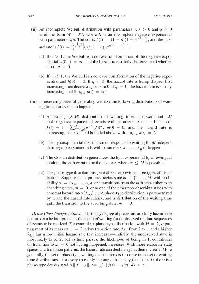
(ii) An incomplete Weibull distribution with parameters γ, λ > 0 and q ≥ 0 is of the form W = X γ , where X is an incomplete negative exponential with parameters λ, q . The cdf is F(t) = (1 − q)(1 − e −λ t 1/γ ) , and the haz-

ard rate is h(t) = λ __ γ t 1−γ ____ γ [(q / (1 − q)) e λ t 1/γ + 1]

−1 .

(a) If γ > 1 , the Weibull is a convex transformation of the negative expo-nential, h(0+) = ∞ , and the hazard rate strictly decreases to 0 whether or not q > 0 .

(b) If γ < 1 , the Weibull is a concave transformation of the negative expo-nential and h(0) = 0 . If q > 0 , the hazard rate is hump-shaped, first increasing then decreasing back to 0 . If q = 0 , the hazard rate is strictly increasing, and lim t↑∞ h(t) = ∞ .

(iii) In increasing order of generality, we have the following distributions of wait-ing times for events to happen.

(a) An Erlang (λ, M) distribution of waiting time: one waits until M i.i.d. negative exponential events with parameter λ occur. It has cdf F(t) = 1 − ∑ m=0

M−1 1 __ m ! e −λt (λt) m , h(0) = 0 , and the hazard rate is

increasing, concave, and bounded above with lim t↑∞ h(t) = λ .

(b) The hypoexponential distribution corresponds to waiting for M indepen-dent negative exponentials with parameters λ 1 , … , λ M to happen.

(c) The Coxian distribution generalizes the hypoexponential by allowing, at random, the m th event to be the last one, where m ≤ M is possible.

(d) The phase-type distributions generalize the previous three types of distri-butions. Suppose that a process begins state m ∈ {1, … , M} with prob-ability α = ( α 1 , … , α M ) , and transitions from the m th state either to an absorbing state, m = 0 , or to one of the other non-absorbing states with constant hazard rates ( λ m, i ) i≠m . A phase-type distribution is parametrized by α and the hazard rate matrix, and is distribution of the waiting time until the transition to the absorbing state, m = 0 .

Dense Class Interpretations.—Up to any degree of precision, arbitrary hazard rate patterns can be interpreted as the result of waiting for unobserved random sequences of events to be realized. For example, a phase-type distribution with M = 2 , α put-ting most of its mass on m = 2 , a low transition rate, λ 2, 1 from 2 to 1 , and a higher λ 1, 0 has a low initial hazard rate that increases—initially, the unobserved state is most likely to be 2 , but as time passes, the likelihood of being in 1 , conditional on transition to m = 0 not having happened, increases. With more elaborate state spaces and transition patterns, the hazard rate can decline again, then increase. More generally, the set of phase-type waiting distributions is L 1 -dense in the set of waiting time distributions—for every (possibly incomplete) density f and ϵ > 0 , there is a phase-type density g with ǁ f − g ǁ 1 := ∫ 0

∞ | f(s) − g(s) | ds < ϵ .


Updating Interpretations.—There are also a wide variety of mixture model or updating interpretations of hazard rates.

If β is a prior distribution on the set of possible distributions of the next arrival time in (0, ∞] , denoted β ∈ Δ(Δ(0, ∞]) , then the hazard rate at t is

(8) h β (t) = lim δ↓0

( 1 _ δ ∫ Δ(0,∞] p((t, t + δ)) dβ( p)) / ( ∫ Δ(0,∞]) p((t, ∞]) dβ( p)) .

If β and β ′ are two priors with h β ( · ) = h β ′ ( · ) , then the optimal course of action is the same so that hazard rate analyses can cover a very broad array of models.

Known Hazard Rates: With δ t denoting point mass on t , if β({ δ t : t ∈ A}) = ∫ A f(x) dx , then h β (t) is the hazard rate associated with the density f( · ) , yielding an interpretation of a known hazard rate.

Bi-modal Hazard Rates: In our models of constitutional amendments, bi-modal hazard rates for reversals of opinions are of interest. They can be understood as a mixture of three effects: with probability α 1 > 0 , the previous change was a fad, and the density for the reversal time of fads is given by f 1 with a low upper bound to its support; with probability α 2 > 0 , it is a longer lasting but still tem-porary change, and the density, f 2 , of such reversals puts mass on a much longer set of times; and with probability q > 0 , there is never a reversal. The hazard rate is initially high, tails off, increases, then decreases again as the probability that W = ∞ given W > t converges to 1 as t ↑ .

Smooth Mixtures: Mixtures of smooth classes of distributions are often dense. For example, if W is an incomplete Weibull distribution with parameters λ, γ, q where (λ, γ, q) is itself random with mixture distribution β , then the class of densities that W may have is again L 1 -dense.12

Interpretations with Expanded State Spaces.—The passage of time, changes of the state, and changes of actions contain information about the distribution of future developments. Adding more states allows one to expand the set of dynamic factors that are modeled: if the state i k contains information about how many localities and/or states have approved womens’ suffrage, then every time this number increases, we expect that the future hazard rate path for opinion reversal should be lower; if the state contains information about how many times a unit has been repaired or upgraded rather than replaced, then every time this number increases we expect the new hazard rate path for a breakdown should be higher than the previous hazard rate path in repair/replace models; if the state contains informa-tion about the number of unsuccessful job interviews, then every time this number increases, we might expect the hazard rate of the distribution of a good job offer to decline.

12 Proofs of such can be given using the approximation techniques in (Hornik et al. 1994). See Cho and White (2010) for references to mixture models of exponentials and Weibulls in both financial econometrics and in duration models.


C. Controlled Semi-Markov Processes

There is a compact state space, S , with metric D S , generic elements denoted i, j, i 0 , i 1 , … , and generic random elements of S will be denoted I k , k = 1, 2, … . There is also a compact action space, A , with generic elements denoted a, b, a 0 , a 1 , … . As above, Y k , k = 0, 1, … are the random variables giving the state-change times, and a stochastic interval is a subset of Ω × [0, ∞) of the form [ [ Y k , Y k+1 [ [ := {(ω, t) : Y k (ω) ≤ t < Y k+1 (ω)} .

We first define the class of plans/policies, their associated outcomes and utilities, and then the stochastic structure, that is, the determinants of the joint distributions of the Y k and the states, I k .

Semi-Markovian Plans.—We use functions 𝔭 : [0, ∞) → A , to specify the cho-sen plan of action within a stochastic interval. We measure distance between plans using the Hausdorff distance between (the closures of) their graphs in a fashion less sensitive to differences in the right tails of the plans. Specifically, we introduce a distance D( · , · ) between points (t, a) and ( t ′ , a ′ ) in [0, ∞) × A that takes the form13 D((t, a), ( t ′ , a′)) = (| e−ρt − e −ρt ′ | + ǁ e −ρt a − e −ρt ′ a ′ ǁ ) in the case that A is a compact subset of ℝ

ℓ . The distance between 𝔭 ∈ ℙ(i, a) and 𝔭′ ∈ ℙ(i′, a′) is defined as

(9) d H (𝔭, 𝔭′ ) = inf {ϵ > 0 : gr(𝔭) ⊂ gr(𝔭′ )ϵ and gr(𝔭′ ) ⊂ gr (𝔭) ϵ } ,

where gr(𝔭) and gr(𝔭′ ) are the graphs of the plans and gr (𝔭) ϵ and gr(𝔭′ )ϵ are the sets of points at D -distance less than ϵ from the graphs.

This metric has the property that differences in the right tails are down-weighted. For example, if r is the diameter of A and e −ρT < ϵ /max (r, 1) , then two plans that disagree only on [T, ∞) can be at d H -distance no more than ϵ from each other. In particular, this means that the set of plans with successive changes of action at least τ > 0 from each other is compact.

DEFINITION 1: A plan starting from ( i 0 , a 0 ) is a function 𝔭 : [0, ∞) → A that sat-isfies 𝔭(0) = a 0 , is piecewise-constant, continuous from the left, and has at most finitely many discontinuities over any finite interval. The set of feasible plans is a non-empty set of plans denoted ℙ( i 0 , a 0 ) where the correspondence from ( i 0 , a 0 ) to ℙ( i 0 , a 0 ) is assumed continuous, and compact-valued and all members of the set are assumed to have a uniformly bounded number of changes of action. A complete semi-stationary plan is a measurable selection from the set of feasible plans, that is, a measurable function from state-action pairs to plans, ( i 0 , a 0 ) ↦ 𝔭 ( i 0 , a 0 ) ∈ ℙ( i 0 , a 0 ).

For 𝔭 ∈ ℙ( i 0 , a 0 ) , T 𝔭 = {t ∈ [0, ∞) : 𝔭(t) ≠ 𝔭(t+)} denotes the finite set of planned action change times (where 𝔭(t+) := lim ϵ↓0 𝔭(t + ϵ) ). The “continu-ous from the left” aspect of plans accommodates instant reactions to changes of states—a plan that instantly changes to an action a 1 in response to a state change

13 That is, has the same uniformity as. See the online Appendix for the general definition.


to ( i 0 , a 0 ) has 0 ∈ T 𝔭 , satisfies 𝔭(0) = a 0 and 𝔭(0+) = a 1 . We interpret the times in T 𝔭 as specifying the chosen action as a function of the within interval time, that is, as a function of the time since the last state change. Formally, for A k := {ω : Y k (ω) < ∞} , ω ∈ A k and t ∈ [ Y k (ω), Y k+1 (ω)) , the within inter-val time s is given by s k (ω, t) = t − Y k (ω) . Using 𝔭 from an interval starting in ( i k , a k ) at time Y k corresponds to changing actions at the within-interval times s k with 𝔭( s k ) ≠ 𝔭( s k +) .

The feasibility constraint is a flexible modeling tool: irreversibility of the action change after, say, changing from ( i 0 , a 0 ) to a 1 is modeled by ℙ( i 0 , a 1 ) containing only the plan satisfying 𝔭(t) ≡ a 1 ; a minimal reaction time of r times involve 𝔭(t) = a 1 for all t ∈ [0, r] .

The Stochastic Structure.—We now specify the density and conditional change probabilities as functions of the past history that satisfy two kinds of continuity conditions, one to guarantee the validity of the Euler equations in Theorem 2 and one to guarantee the existence of optima in the Bellman equation in Theorem 1. In the following, the distance between densities, complete or not, is the L 1 distance, ǁ f − g ǁ 1 = ∫ 0

∞ | f (s) − g(s) | ds .

DEFINITION 2: A semi-Markovian stochastic structure is a function (s, 𝔭, i) ↦ ( f (s; 𝔭, i), μ(s; 𝔭, i)) from (0, ∞) × ℙ × S to [0, ∞) × Δ(S) satisfying the follow-ing conditions:

(i) Progressivity, for all state-action pairs (i, a) , all 𝔭, 𝔭′ ∈ ℙ(i, a) and all intervals [0, t] , if 𝔭 |[0, t] = 𝔭 |[0, t] ′ , then for all s ∈ [0, t] , ( f (s; 𝔭, i), μ(s; 𝔭, i)) = ( f (s; 𝔭′, i), μ(s; 𝔭′, i)) ;

(ii) Joint and L 1 -continuity, (s, 𝔭, i) ↦ ( f (s; 𝔭, i), μ(s; 𝔭, i)) is jointly continu-ous, and (𝔭, i) ↦ f ( · ; 𝔭, i) is L 1 -continuous; and

(iii) Non-redundancy, for all s , μ(s; 𝔭, i)({i}) ≡ 0 .

Using a plan 𝔭 ∈ ℙ( i k , a k ) in an interval [ [ Y k , Y k+1 [ [ that starts in ( i k , a k ) means that the waiting time, W k+1 := Y k+1 − Y k , has the possibly incomplete density f (s; 𝔭, i k ) on (0, ∞) , and the distribution of the waiting time must be L 1 -continuous in the chosen plan and starting state. Unbounded densities, such as the Weibulls with f (0+) = h(0+) = ∞ , are allowed because the continuity is only required on (0, ∞) . While densities are required to be continuous on the within-interval time (0, ∞) when there is no change in action, continuity in plans allows for the density and the change probability to be discontinuously different before and after a change in action.14 Conditional on W k+1 = w < ∞ , the distribution of the new state is given by μ(w; 𝔭, i k ) , and non-redundancy requires changes in states to actually be changes. The progressivity condition guarantees that only past changes in actions and states can affect the current density and conditional change probability.

14 An example of an allowed discontinuity in the density is in equation (1), specifying the stochastics for the inoculation model.


The following specifies how plans interact with stochastic structures to give rise to distributions of waiting times and state changes. Recall the convention that min ∅ = ∞ .

DEFINITION 3: Using a plan 𝔭 0 ∈ ℙ( i 0 , a 0 ) starting from ( i 0 , a 0 ) at Y 0 = 0 gives rise to a random waiting time-state pair, ( W 1 , I 1 ) with the induced distribution, possibly incomplete, defined by ν 1 (E × F) = ∫ E f (s; 𝔭 0 , i 0 ) · μ(s; 𝔭 0 , i 0 )(F) ds for E × F ⊂ (0, ∞) × S . For k ≥ 1 , if W k = w k < ∞ , a k = 𝔭 k−1 ( W k ) and I k = i k , using a plan 𝔭 k ∈ ℙ( i k , a k ) gives rise to a random waiting time-state pair, ( W k+1 , I k+1 ) with the induced distribution ν k+1 (E × F) = ∫ E f (s; 𝔭 k , i k ) · μ(s; 𝔭 k , i k )(F) ds . Continuing inductively, a sequence of plans 𝔭 0 , 𝔭 1 , … with 𝔭 k ∈ ℙ( i k , 𝔭 k−1 ( W k )) gives rise to a sequence of conditionally independent random waiting times-states pairs, ( W k , I k ) , k = 1, … , K , with K := min {k : W k = ∞} .

For any semi-stationary plan, i.e., any measurable function (i, a) ↦ 𝔭 (i, a) ∈ ℙ(i, a) , the induced distribution of ( W k , I k ) depends only on the value of I k−1 and 𝔭 k−1 ( W k ) . Therefore, the induced distributions for a complete semi-stationary plan give a stochastic kernel (Feller 1971, VI.11, Definition 1) so that the process ( W k , I k ) , k = 1, … , K is a Markov chain with a random, possibly infinite, number of realizations. Theorem 1 will show that semi-stationary plans are optimal.

Utilities.—Changing action from a to b in state i has a cost, c(a, b; i) . We assume that c : (A × A) × S → ℝ ++ is continuous, has a strictly positive minimum value, and that direct changes are always cheaper than multi-step changes of action, c(a, a ′ ; i) + c( a ′ , a′′; i) > c(a, a′′; i) . Flow utilities are given by a continuous u : S × A → ℝ. For an interval starting in (i, a) , the utility associated with a plan 𝔭 ∈ ℙ(i, a) has two components, the expected flow utility,

(10) ∫ 0 ∞

[ ∫ 0 s u(i, 𝔭(t)) e −rt dt ] f (s; 𝔭, i) ds,

and, with T 𝔭 denoting the action change times, the expected costs,

(11) ∫ 0 ∞

[ ∑ t∈ T 𝔭 , t<s

c(𝔭(t), 𝔭(t+); i) e −rt ] f (s; 𝔭, i) ds .

We denote the sum of the terms in (10) and (11) by (𝔭; (i, a)) so that the utility of a sequence of plans 𝔭 0 , 𝔭 1 , … starting in ( i 0 , a 0 ) at Y 0 = 0 is

(12) ( 𝔭 0 ,( i 0 , a 0 )) + E e −r Y 1

( 𝔭 1 ,( I 1 , 𝔭 0 ( Y 1− , Y 0 ))) + ⋯,

where the expectations of the I k and the e −r Y k are taken with respect to the distribu-tions induced by the plans, and we assume that 𝔭 k ∈ ℙ( I k , 𝔭 k−1 ( Y k − Y k−1 )) because this is the state-action pair in effect when the state change at Y k happens.


D. Existence and the Bellman Equation

The value function for an sMdp, V * : S × A → ℝ , is defined as

(13) V * ( i 0 , a 0 ) = sup 𝔭 0 , 𝔭 1 , …

( 𝔭 0 ( i 0 , a 0 )) + ∑

k≥1

E e −r Y k

( 𝔭 k ;( I k , 𝔭 k−1 ( Y k − Y k−1 ))

where 𝔭 0 ∈ ℙ( i 0 , a 0 ) and 𝔭 k ∈ ℙ( I k , 𝔭 k−1 ( Y k − Y k−1 )) for k ≥ 1 . The following par-allels the existence results for discrete time dynamic programming in Blackwell (1965, Section 6).

THEOREM 1: For an sMdp, the mapping T : C(S × A) → C(S × A) defined by

(14) T(V )(i, a) = max 𝔭∈ℙ(i, a)

[(𝔭;(i, a)) + ∫ (0, ∞)×S

V(i, 𝔭(s)) e −rs d v 𝔭 (s, i)]

has contraction factor at most β := su p (i, a),𝔭∈ℙ(i, a) ∫ 0 ∞ e

−rs f (s; 𝔭, i) ds < 1,

its unique fixed point is the value function, V ∗ , and following the complete semi-stationary plan given by the arg max policy for (14) in every stochastic inter-val delivers expected payoffs V ∗ (i, a) for every (i, a) ∈ S × A .

Thus, the stochastic intervals deliver the recursive structure that allows us to use semi-stationary plans to solve the problem in (13): if one leaves a stochastic interval [ [ Y k , Y k+1 [ [ to the state I k+1 while taking an action a k , one starts the new stochastic interval in the state-action pair ( I k+1 , a k ) ; if one behaves optimally thereafter, one receives V ∗ ( I k+1 , a k ) e −r Y k+1 ; and this is the maximization problem in (14). In the proof, the assumption that costs are bounded away from 0 is used only to guarantee that only a compact set of plans need be considered. As an immediate corollary, if the feasible set of plans is already compact, the assumption that costs be bounded from 0 is not needed and the same result holds.

E. Euler Equations

We now turn to the FOCs and SOCs for finite but strictly positive delay to be optimal for those intervals in which one change of action is optimal. Here we restrict attention to models in which the optimality conditions for a t 1 ∗ ∈ (0, ∞) involve only the value function and properties of the stochastic structure at t 1 ∗ . For plans with only one action change at t 1 , we can express the stochastic structure as a function w ↦ ( f (w; t 1 ), μ(w; t 1 )) . Progressivity requires the existence a function w ↦ ( f − (w), μ − (w)) such that for all w < t 1 < t 1 ′ , ( f (w; t 1 ), μ(w; t 1 )) = ( f (w; t 1 ′ ), μ(w; t 1 ′ )) = ( f − (w), μ − (w)) . For t 1 < t 1 ′ < w we can have ( f (w; t 1 ), μ(w; t 1 )) ≠ ( f (w; t 1 ′ ), μ(w; t 1 ′ )) , which means that the general FOCs for an optimal t 1 ∗ must involve the discounted future path of the derivative of ( f ( · ; t 1 ∗ ), μ( · ; t 1 ∗ )) . These are non-local aspects of the future that are not captured by the value function. The following is a minimal assumption for FOCs and SOCs to involve only the value function and properties of the stochastic structure local to t 1 ∗ .


DEFINITION 4: A stochastic structure is localized if for all starting points ( i 0 , a 0 ) and a 0 to a 1 changes, there exists a function w ↦ ( f + (w), μ + (w)) such that ( f (w; t 1 ), μ(w; t 1 )) = ( f (w; t 1 ′ ), μ(w; t 1 ′ )) = ( f + (w), μ + (w)) for all 0 < t 1 < t 1 ′ < w .

We use h + (w) and E + to denote the hazard rate and the expectation operator for μ + (w) at times w > t 1 , and use h − (w) and E − (w) to denote the corresponding quantities for w < t 1 .

THEOREM 2: In an sMdp with a localized15 stochastic structure, if 𝔭 ∗ solves

(15) max 𝔭∈ℙ( i 0 , a 0 )

[(𝔭;( i 0 , a 0 )) + ∫ (0, ∞)×S

V*(i, 𝔭(s)) e −rs d v 𝔭 (s, i)] ,

and hesitates until a time t 1 ∗ ∈ (0, ∞) for its single action change to a 1 ∗ at cost c ∗ , then t 1 ∗ must satisfy

(16) rc* − [u( i 0 , a 1 * ) − u( i 0 , a 0 )]

= h − ( t 1 * ) ( 1 __ r u( i 0 , a 1 * )(1 − γ( t 1 * )) + [γ( t 1 * ) E + V * ( I 1 , a 1

* ) − E − V * ( I 1 , a 0 )] − c * ) ,

where γ( t 1 ∗ ) := h + ( t 1 ∗ ) ____ h − ( t 1 ∗ ) . Further, if the term multiplying h − ( t 1 ∗ ) in (16) is positive

(resp. negative), then the SOCs are strictly satisfied if and only if the hazard rate h − is increasing (resp. decreasing) at t 1 ∗ .

The class of problems for which this is applicable models situations where: there is only one realistic opportunity for a change of action; or the cost of changes is high relative to the differences in the flow utility; or when uncertainty about the durability of the circumstances pushing one to change actions is initially high but then settles down for good. A broad class of institutional decision making problems fit these descriptions. Examples below demonstrate that the one-move necessary condition in (16) can also be useful when several moves are optimal within an interval and when the choice of possible action is continuous rather than discrete.

IV. Applications of the Bellman and Euler Equations

The increasing and decreasing hazard rates cases in Theorem 2 have very different intuitions, one consonant with the searching till success seems too unlikely, the other consonant with delaying expensive preventive measures until danger presses. To see this in more detail, we now examine the Euler equations in various models, starting with the simplest, and proceeding through their use in models that include multiple

15 The FOCs for non-localized stochastic structures can be found in the online Appendix.


action switches within a stochastic interval and continuous choices of action. We then turn to an analysis of optima based more directly on the Bellman equations.

A. Memoryless Processes

When f ( · ; 𝔭, i) , the density part of the stochastic structure has a constant hazard rate between action changes and change probability, μ( · ; 𝔭, i) , is constant except, possibly, at action changes, the right-hand side of the Euler equation, (16), is con-stant for any choice of a 1 ∗ . Within this class of problems, at most one change of action is ever optimal, and there are three possibilities for the optimal hesitation.

First, if flow benefits to the best change of action outweigh the benefits of delay, that is if the left-hand side of (16) is larger than the right-hand side, then t 1 ∗ = 0 . Further, because the hazard rates and transition probabilities are constant, if this is true at any t 1 , then it is true for all t 1 .

Second, if the benefits of delay outweight the flow benefits of the best change of action, then the optimal t 1 ∗ = ∞ because the right-hand side of (16) is larger than the left-hand side. Again, if this is true at any t 1 , then it is true for all t 1 .

Third, if we have equality in (16), then any t 1 ∗ ∈ [0, ∞] is optimal.

B. Two Types of Search

A standard search procedure often starts with a quick scan which will find any-thing obvious, and, if this is not successful, then moves on to a slower, more thorough search. We first review the simple search model above then extend it to encompass the quick-scan-then-grind search model. The model of Section IIA has two states, i 0 , no search results, and i 1 , successful search; and two actions, s 0 , searching, and b , abandoning search. The set of feasible plans is D -compact: it has ℙ( i k , s 0 ) being the set of all functions taking the value s over some interval [0, t 1 ] , t 1 ∈ [0, ∞] , and taking the value b thereafter, k = 0, 1 ; and, to capture irreversibility, has ℙ( i k , b ) being the set of all functions constant at b . The density before t 1 is given by f ( · ) , after the change to b , it is given by f ( · ; t 1 ) ≡ 0 so that the post- to pre-change hazard ratio is γ( t 1 ) = 0 . The flow utilities are u( i 0 , s 0 ) = −c , u( i 0 , b) = π _ , u( i 1 , s 0 ) = _ π − c and u( i 1 , b) = _ π . Change costs are set equal to 0 . With these choices, the FOCs from Theorem 2 are

(17) 0 − [ π _ + c] = h − ( t 1 * ) ( 1 __ r u( i 0 , b)(1 − 0) + [0 E + V * ( I 1 , b) − E − V * ( I 1 , s 0 )] − 0) .

Since the only possible change of state is from i 0 to i 1 , the new state, I 1 is, with prob-ability 1 , equal to i 1 so that E − V * ( I 1 , s 0 ) is equal to 1 _ r

_ π , the expected discounted value of the flow of _ π . With these, the FOCs are h( t 1 ∗ ) = r(c + π _ )/ ( _ π − π _ ) and the SOCs require h 1 ( t 1 ∗ ) < 0 .

Suppose now that there are two search techniques: s 1 with flow costs c 1 and haz-ard rate h 1 that starts high, quickly declines to 0 and has ∫ 0

∞ h 1 (x) dx < ∞ , that is, a strictly positive incompleteness parameter; and s 2 with corresponding c 2 and h 2


that declines much more slowly and has ∫ 0 ∞ h 2 (x) dx = ∞ . Suppose further that

switching from s 1 to s 2 at t 1, 2 means that the hazard rate at t 1, 2 + s is h 2 (s) , that the value if only s 2 is available is V 2 > 1 _ r π _ , and that it is optimal to use s 1 first. The

FOCs for t 1, 2 ∗ are h 1 ( t 1, 2 ∗ ) = r( c 1 + r V 2 ) _______ _ π − r V 2 because r V 2 is the annuitized flow value

of V 2 . As the SOCs are h 1 ′ ( t 1, 2 ∗ ) < 0 , the comparative statics are straightforward: increases in r , i.e., becoming less patient, means more time spent on scanning, that is, more time hoping for a quick resolution; increases in c 1 or V 2 as well as every-where decreases in h 1 mean less time spent scanning.

The hazard rate at t 1, 2 + s being h 2 (s) is an independence assumption that may not make sense if the distributions are incomplete and our interpretation of incom-plete distributions for search times is that the object is not there to be found.16 One can capture and analyze such a situation by using V 2 ( q t ) in the FOCs where q t is posterior probability that the object is not findable using s 2 given that using s 1 until t has not found the object and V 2 ( q t ) is the value to using s 2 starting from that point.

C. Continuous Degrees of Inoculation

In the simple inoculation model of Section IIB there are: two states, i 0 , the crisis not having arrived, and i 1 , the crisis having arrived; and two actions, a 0 , not inocu-lating, and a 1 , inoculating. The cost of switching from a 0 to a 1 is C , the pre-disaster flow utilities are u( i 0 , a 0 ) = u( i 0 , a 1 ) = _ u , while the post-disaster flows depend on whether or not one was inoculated, u( i 1 , a 0 ) = 0 and u( i 1 , a 1 ) = u _ , _ u > u _ > 0 . To capture inoculation being useless after the disaster has arrived, it is simplest to specify that ℙ( i 1 , a 0 ) contains only the time path constant at a 0 . The arrival density at times w prior to inoculation at t 1 is f(w) , at w ≥ t 1 , it is (1 − θ) f (w) so that the post- to pre-hazard rate ratio is γ( t 1 ) = (1 − θ) . With these, the FOCs from Theorem 2 are

(18) rC − [ _

u − _

u ]= h − ( t 1 * ) ( 1 __ r _

u θ + [(1 − θ) E + V * ( I 1 , a 1 ) − E − V * ( I 1 , a 0 )] − C) .

Having inoculated when the state change I 1 = i 1 arrives yields expected discounted payoffs of E + V * ( I 1 , a 1 ) = 1 _ r u _ , having failed to inoculate by that time yields E − V * ( I 1 , a 0 ) = 0. Combining, the FOCs are h( t 1 ∗ ) = rC / ( 1 _ r [θ

_ u + (1 − θ) u _ ] − C ) , the SOCs are h 1 ( t 1 ∗ ) > 0 , and increases in either θ or u _ make less hesitation optimal.

Let us now suppose that the benefits of inoculation, the efficacy, θ , and the post-disaster utility, u _ , are continuously adjustable, and that their cost is C(θ, u _ ) . In this context, optimal design of the inoculation equates expected marginal costs and benefits. With C u _ du denoting the cost of increasing u _ by du , the optimal choice of u _ equates the marginal cost, C u _ , with the expected value of the increased flow of utility if inoculation precedes disaster, C u _ = (1 − θ ∗ ) 1 _ r E( e −r(W− t 1

* ) | W > t 1 * ) , and the optimal θ ∗ equates the marginal cost of prevention to the discounted expected value of avoiding the disaster, C θ = (

_ u − u _ * ) 1 _ r E( e −r(W− t 1

* ) | W > t 1 * ) . These FOCs

16 Different search techniques can be blind in different ways, so “not being findable using s 1 ” need not have implications for the likelihood of “not being findable using s 2 .”


yield the following conclusions: increases in one aspect of the quality of an inocula-tion lower the marginal value of the other aspect; irrespective of the distribution of (W | W > t 1 ) , the (absolute value of the) slope of the iso-cost curve at the optimum is C θ / C u = (1 − θ ∗ ) / ( _ u − u _ ∗ ) ; and the signs of comparative statics results for θ ∗ and u _ ∗ must be equal, θ ∗ and u _ ∗ increase with more patience (lower r ), with more at stake (higher _ u ), and with a more hazardous environment (an everywhere increase in hazard rate).

D. Revisiting Adaptation to Changing Circumstances

Taking voting rights away from a newly enfranchised group that can vote against being disenfranchised is difficult in a democracy.17 By contrast, restoring privileges that have been taken away, such as the legal consumption of alcohol, seems relatively easy. We first use the Euler equations for the model of optimal adaptation to ever changing circumstances of Section IID to show that higher costs of either passing or repealing an Amendment lead to more hesitation (one can also use the Bellman equa-tions for this). We then show that, in many but not all cases, if passage of a law reduces the hazard that opinion will switch against it, this decreases optimal hesitation.

The Costs of Repeal.—Recall that the two matched state-action pairs, (i, a) and ( j, b) give positive flow utilities, while the mismatched pairs, (i, b) and ( j, a) , give flow utilities of 0 . In either matched state-action pair, there is no incentive to incur the cost of changing action so that the Euler equations are never satisfied. For the mismatched pair (i, b) , provided that γ(t) = 1 , the Euler equation is

(19) [rc(b, a; i) − u(i, a)] = h i ( t i ) (0 + [ V ∗ ( j, a) − V ∗ ( j, b)] − c(b, a; i)) ,

with a similar expression for the t j ∗ associated with the other mismatched pair, ( j, a) .

Since rc(b, a; i) < u(i, a) is necessary for it ever to be optimal to switch actions, if the Euler equations are satisfied, then both sides of (19) are negative and the SOCs require the hazard rate to be decreasing. Rewriting with the hazard as a ratio of two positive numbers we have

(20) h i ( t i ∗ ) = u(i, a) − rc(b, a; i) ______________________ [ V ∗ (j, b) − V ∗ (j, a)] + c(b, a; i) .

Since the hazard rates must be decreasing, the direct effect of an increase in c(b, a; i) is to require more delay, that is, a higher t i ∗ . There are also indirect effects of increases in either c(b, a; i) , the cost of passing an Amendment, or of increases in c(a, b; j) the cost of repealing an Amendment, but these indirect effects also push for more delay. Increases in the change costs decrease all of the values, but, e.g., in (20), the dif-ference, [ V ∗ ( j, b) − V ∗ ( j, a)] , increases as the action change costs increase— ( j, b) is a matched pair so no change will occur in the stochastic interval beginning at

17 Witness the decades of effort to disenfranchise freedmen in the southern United States after the passage of Amendment XV granting suffrage to former (male) slaves.


( j, b) while the pair ( j, a) is mismatched. With declining hazard rates, the larger delays correspond to waiting until one is more sure that any future change of opinion will not happen, or is, at least, further in the future.

The Power of Laws to Affect Attitudes.—Several contemporary sources suggest that both the opponents and proponents had believed, mistakenly as it turns out, that in the event Prohibition was adopted, the laws would be widely followed and the social norm would also switch in the direction of temperance. In the model, this corre-sponds to lowering the post-change hazard rate for a switch back to the status quo ante. Intuitively, this pushes for less hesitation because a swifter passage of the amendment allows one to “lock in” the benefits of having the action match the present state. In the model, this is true for a wide range of cases, but not in complete generality.

Recall that different matched state-action pairs have different flow utilities. If these flow utilities are approximately equal, as we think reasonable for the present application, or if being matched in the present state is more valuable than being matched in the other state(s), then acting so as to get the lock-in is optimal. However, if being matched to the present state is very much less desirable than being matched in the other state(s), locking in corresponds to choosing a long time at a very low level of utility, and this can be suboptimal. In terms of the FOCs from Theorem 2, this corresponds to the negative term multiplying h − ( t 1 ∗ ) being very large in absolute value, meaning that it is optimal to delay until the hazard rate for future change is very low indeed.

V. Conclusions and Extensions

We began with the question as to what the optimal time is for changing a status quo policy in response to a change of the environment when policy change is costly and there is the possibility of subsequent changes in the environment. The trade-off is between optimizing with respect to the current state and optimizing with respect to the expected future state when the passage of time contains information about how soon the next change is likely to occur and what it is likely to entail. The Euler equations of Theorem 2 for the optimal amount of hesitation before a change of policy contain information about the optimal time, how that optimal time interacts with the new action, and how it interacts with different hazard rate patterns.

A. Decreasing Hazard Rate Problems

Every instant of hesitation in matching the current action to the current state has an opportunity cost, but with a decreasing hazard rate, hesitation increases the likelihood that any change of action will be enduring. When the costs of changing action, or of changing it back, are higher, this kind of “informative waiting” is more valuable, an observation that contains some insights into the examples presented at the beginning, and suggests other areas of applicability.

Prohibition and women’s suffrage have an intimately tied history with large over-lap among the activists promoting both Amendments (Flexner and Fitzpatrick 1996). Our model suggests two cost-based explanations for the passage of Amendment XVIII (Prohibition) and XIX (Suffrage). Prohibition was passed three years after


Amendment XVI, which allowed the federal government to collect income taxes. By providing an alternative to the large tax receipts from alcohol, this drastically lowered the cost of Prohibition, lowering the “optimal” delay. Perhaps contributing to this effect was the widespread belief that, if passed, temperance would become the new norm. Women’s suffrage was delayed long past the accumulation of a great deal of evidence of majority approval, and part of the delay may be explained as “optimality” in the face of the high costs of reversing any enfranchisement.

A fascinating institutional design question is how much delay to build in. In Federalist 62, James Madison (Fairfield 1966) argued for “The necessity of a sen-ate” with “tenure of considerable duration” because of “the propensity of all single and numerous assemblies to yield to the impulse of sudden and violent passions, and to be seduced by factious leaders into intemperate and pernicious resolutions.” From the point of view of the model here, “intemperate and pernicious resolutions” cor-respond to actions that are either very costly or very costly to reverse, and “sudden and violent passions” correspond to changes of state that have high hazard rates for reversal, both of which lead to larger optimal delays.

B. Increasing Hazard Rate Analyses

While the previous models have a common intuition about trading off the infor-mative value of waiting against the opportunity cost of immediate action, an entirely different class of intuitions is at work when hazard rates are increasing.

The costs of inoculation against financial system crises are, politically at least, very high. Our investigation of the optimal delay highlights the trade-off between interventions that lower the arrival rate of the next crisis and those that lower the damage that it will cause: a policy change that reduces one of these makes the other less valuable at the margin. In such cases, hesitation saves incurring the cost of inoculation, but becomes suboptimal as the hazard rate rises and the danger comes closer, an issue that seems relevant to policy responses to international conflicts and to climate change.

Issues of limitations on executive power, especially with respect to war, have been discussed, at least since the invention of the telegraph, in terms of the need for quick decisions. The Vietnam war, the Watergate scandal—neither led to any particularly extensive checks on, or built-in delays to the use of, executive power (though there is debate about the legality and effects of the War Powers Act). From the point of view of the model here, this is optimal if delays in changing policy in the face of increasing danger are very costly, if prompt action is a form of inoculation against future disas-ters in the context of spiking hazard rates. This seems a good description of many of the international relations problems the executive branch is called on to solve.

C. Our Methodology in Perspective

Our interest throughout has been focused on the optimal timing of discrete changes of action. There is a part of the semi-Markovian decision theory literature that studies continuously adjustable controls: Stone (1973) gives a differential inclu-sion condition for the value function when actions are continuously adjustable and control both transition times and distributions; Doshi (1979) generalized this work


to models in which the states not only follow jump processes but may also have a diffusion-like component. The modeling trade-offs are between discrete changes and their costs, which is our focus, versus continuous adjustability of a policy, which is theirs. This is reflected in the solutions methodologies: FOCs and more analytic tractability in our approach; the near necessity for numerical solutions characterized by differential inclusions in theirs.

An interesting perspective that sheds light on the approach taken here is in Ghosh and Saha (2012), who reduce sMdps with continuously adjustable controls to embedded discrete-time Markovian decision problems with compact action spaces representing the set of measurable time paths of the control variables. For station-ary, discrete-time Markovian decision problems, in state z k in the k th period, the value, v( z k ) , is the maximum, over available actions, a k ∈ A( z k ) , of the expected one period reward, r( a k , z k ) , plus the expected discounted (at rate δ ) value of the state in one period, δE (v( z k+1 )| z k , a k ) . In our sMdps: being in z k in the k th period is replaced with being in the state-action pair ( i k , a k ) at the beginning of the k th sto-chastic interval, [ [ Y k , Y k+1 [ [ ; the set of actions becomes the set of plans 𝔭 ∈ ℙ( i k , a k ); r( a k , z k ) becomes the expected payoffs over the interval [ [ Y k , Y k+1 [ [ ; and the expected discounted value of the state in one period becomes the expected discounted value of V ∗ ( I k+1 , 𝔭( Y k+1 − Y k )) e −r Y k+1 because 𝔭( Y k+1 − Y k ) is the action being used as Y k+1 arrives. Theorem 1 shows that one can reduce the problem to the sequence of problems encountered at the beginning of the intervals. This directly parallels Theorem 3.1 in Ghosh and Saha (2012), who take the set of actions to be the set of progressively measurable, continuous time control paths as opposed to our ℙ( i k , a k ) , a set of left-continuous piecewise constant functions.

D. Extensions and Further Research

In this paper we have assumed that the decision maker’s knowledge of the sto-chastic structure can be expressed in terms of well-defined probabilities. One set of extensions that we are working on is to incorporate ambiguity into the model and analyze the implications. In real world problems like climate change, where lack of consensus about the exact stochastic structure is a key issue, such an approach seems more reasonable.

Economic models of climate change have traditionally treated the process as one of gradual change to a new, stable state. Recent research in climate science has found evidence of both very rapid changes over a short period of time (around a decade), as well as significant fluctuations or “environmental flickering” over periods as short as a year (Hall and Behl 2006; Stern 2007). These phases of rapid change and/or flick-ering seem to be triggered once a threshold point is reached in the ecological system. Quick changes in climate are more expensive to adapt to, and if we are in a situation where the arrival times of subsequent changes have a range of high arrival rates, the expense is further increased, pushing policy recommendations in the direction of those that arise from some forms of the precautionary principle.18 While “gradual change” models have usually prescribed “adaptation to climate change” as opposed

18 The common core of most variants of the “Precautionary Principle” is that lack of complete understanding of the consequences of actions or policies with significant risk of long term or irrevocable harm is not sufficient reason


to “intervention to avert it” (Nordhaus and Boyer 2003), the decision problem takes a new shape when we incorporate the uncertainty over the expected arrival time of a possible catastrophic change and over the issue of whether or not we are moving toward such a critical threshold. In this context, the cost of controlling the intensity of the arrival rate process, and its interplay with ambiguity and ambiguity aversion need to be factored into any discussion of optimal policy.

Appendix

The arguments here give the essential ideas but suppress many details. These can be found in the online Appendix.

PROOF OF THEOREM 1:We show that the mapping T is well-defined, has the given contraction factor, that

its unique fixed point is the true value function, V ∗ , and that following the argmax policy in (14) delivers V ∗ .

Given the continuity and compact-valuedness of (i, a) ↦ ℙ(i, a) , Berge’s the-orem of the maximum guarantees that T is well-defined provided that the function being maximized in (14) is jointly continuous. There are three parts to the function (𝔭; (i, a)) ↦ [(𝔭; (i, a)) + ∫ (0,∞)×S V(i, 𝔭(s)) e −rs d ν 𝔭 (s, i)] , the flow payoff part and the costs part of ( · ) , and the integrated expected value of V( · , · ) .

• For the flow payoffs, define the uniformly bounded sequence of functions h α by h α (s) = ∫ 0

s u(i, 𝔭 α (t)) e −rt dt and define h(s) = ∫ 0 s u(i, 𝔭(t)) e −rt dt .

The h α converge uniformly to h , hence ∫ h α (s) f α (s) ds → ∫ h(s) f (s) ds . • For the costs part, define g α (s) = ∑ t∈ T 𝔭 α , t<s

c( 𝔭 α (t), 𝔭 α (t + ); i α ) e −rt and

g(s) the corresponding function for (𝔭, (i, a)) . The sequence of functions g α is uniformly bounded, and, by the joint continuity of c( ·, ·; ·) and the joint and L 1 -continuity of f ( ·; ·, ·) , ∫ g α (s) f α (s) ds → ∫ g(s) f (s) ds .

• To show that ∫ (0,∞)×S V( j, 𝔭 α (s)) e −rs d ν 𝔭 α (s, j) converges, note that as a α → a , the functions i ↦ V(i, a α ) converge uniformly to the function i ↦ V(i, a) . The joint continuity of μ( ·; ·, ·) therefore implies that the con-tinuous function s ↦ m α (s) := ∫ S V( j, a α ) e −rs μ(s; 𝔭 α , i α )(dj) converges to the continuous function s ↦ m(s) := ∫ S V( j, a) e −rs μ(s; 𝔭, i)(dj) . Further, joint continuity implies that convergence is uniform over any bounded set of s , and since the function is uniformly less than any ϵ > 0 for all s ≥ T for some T < ∞ , the convergence is in fact uniform over (0, ∞) , hence ∫ 0

∞ m α (s) f α (s) ds → ∫ 0 ∞ m(s) f (s) ds .

From Blackwell’s Lemma for contraction mappings (e.g., Corbae, Stinchcombe, and Zeman 2009, Lemma 6.2.33), to show that T is a contraction mapping with contrac-tion factor β , it is sufficient to show that (i) T is monotonic, and (ii) that for any constant κ ≥ 0 and V ∈ C(S × A) , T(V + κ) ≤ T(V) + βκ . Monotonicity is im mediate.

for refusal to regulate. Though it is the basis of major environmental policy frameworks, e.g., the Kyoto Protocol, the most restrictive versions of the principle have been criticized for not having proper analytical basis (Sunstein 2002).


For (ii), define Ψ(V, 𝔭) = [(𝔭; (i, a)) + ∫ (0,∞)×S V(i, 𝔭(s)) e −rs d ν 𝔭 (s, i)] , let 𝔭 ∗ and 𝔭 κ solve

(A1) max 𝔭∈ℙ(i, a)

Ψ(V, 𝔭) and max

𝔭∈ℙ(i, a)

Ψ(V + κ, 𝔭)

so that Ψ(V, 𝔭 ∗ ) = T(V ) and Ψ(V + k, 𝔭 κ ) = T(V + κ) . By the optimality of 𝔭 κ , Ψ(V + κ, 𝔭 ∗ ) ≤ Ψ(V + κ, 𝔭 κ ) . Further,

(A2) Ψ(V + κ, 𝔭 ∗ ) = Ψ(V) + κ · ∫ 0 ∞

e −rs f (s; 𝔭 ∗ , i) ds .

Define β = sup ∫ 0 ∞ e −rs f (s; 𝔭 ∗ , i) ds . By L 1 -continuity and compactness, the supre-

mum is achieved, hence β < 1 . Combining, T(V + κ) ≤ T(V) + βκ .The arguments for the last two parts of the theorem parallel the standard dis-

crete-time dynamic programming arguments: if V † is the unique fixed point for T , then following the arg max 𝔭 ∗ for the first stochastic interval and receiving V † ( I 1 , a) when the interval ends must have value V † . Therefore following 𝔭 ∗ for the first two stochastic intervals has value V † . Since the strictly positive W k have expec-tation uniformly bounded away from 0 , following 𝔭 ∗ in each interval yields V † . By definition, V ∗ ≥ V † , and if V ∗ ( i 0 , a 0 ) > V † ( i 0 , a 0 ) for some ( i 0 , a 0 ) , then V † is not the fixed point of T . ∎

PROOF OF THEOREM 2: At an optimal 0 < t 1 < ∞ , the difference between the payoff to changing at

t 1 and changing at t 1 + dt , dt ≃ 0 must be equal to 0 . There are four components to the difference: the difference in the annuitized flow cost of the action change, −r c ∗ dt where c ∗ denotes c( a 0 , a 1 ∗ ; i 0 ) ; the difference in flow utility, [u( i 0 , a 1 ∗ ) − u( i 0 , a 0 )] dt ; the difference in the expected value of a state change net of the change cost c ∗ ,

(A3) [ ( ∫ S V(i, a 1 ∗ ) μ + ( t 1 )(di) − c ∗ ) h + ( t 1 ) − ( ∫ S V(i, a 0 ) μ − ( t 1 )(di)) h − ( t 1 )] dt;

and the difference in the expected utilities accrued from the change in the size in the atom at ∞ conditional on the change not having arrived by t 1 ,

(A4) [ ∫ t 1

t 1 +dt ( f − − f + )(s) ds _______________

1 − F( t 1 ) ] u( i 0 , a 1 ∗ ) 1 _ r = [u( i 0 , a 1 ∗ ) 1 _ r ] ( h − ( t 1 ) − h + ( t 1 ))dt .

Adding the terms, setting them equal to 0 and solving yields the FOCs

(A5) h − ( t i ∗ ) = rc* − [u( i 0 , a 1 ∗ ) − u( i 0 , a 0 )] _____________________________________________

1 _ r u( i 0 , a 1 ∗ )(1 − γ( t i ∗ )) + [γ( t i ∗ ) E + V ( I 1 , a 1 * ) − E − V ( I 1 , a 0 )] − c *

,


where γ(t) is defined as the ratio of post- and pre-change hazard rates, γ(t) = h + (t) ____ h − (t) ,

and E − and E + are defined as expectations of the next state, I 1 , under the distribu-tions μ − ( t 1 ) and μ + ( t 1 ) respectively. The arguments for the SOCs and the sign of the derivative of the hazard rate directly parallel the arguments given in Section II. ∎

REFERENCES

Amar, Akhil Reed. 2006. America’s Constitution: A Biography. New York: Random House. Blackwell, David. 1965. “Discounted Dynamic Programming.” Annals of Mathematical Statistics 36

(1): 226–35.Boyarchenko, Svetlana, and Sergei Levendorski ı̆. 2007. Irreversible Decisions under Uncertainty:

Optimal Stopping Made Easy. New York: Springer Berlin Heidelberg. Carmines, Edward G., and James A. Stimson. 1990. Issue Evolution: Race and the Transformation of

American Politics. Princeton, NJ: Princeton University Press. Chintagunta, Pradeep K. 1998. “Inertia and Variety Seeking in a Model of Brand-Purchase Timing.”

Marketing Science 17 (3): 253–70.Cho, Jin Seo, and Halbert White. 2010. “Testing for Unobserved Heterogeneity in Exponential and

Weibull Duration Models.” Journal of Econometrics 157 (2): 458–80.Corbae, Dean, Maxwell B. Stinchcombe, and Juraj Zeman. 2009. An Introduction to Mathematical

Analysis for Economic Theory and Econometrics. Princeton, NJ: Princeton University Press.Diamond, Peter. 2011. “Unemployment, Vacancies, Wages.” American Economic Review 101 (4):

1045–72.Doshi, Bharat T. 1979. “Generalized Semi-Markov Decision Processes.” Journal of Applied Probabil-

ity 16 (3): 618–30.Eichengreen, Barry. 2010. “The Breakup of the Euro Area.” In Europe and the Euro, edited by Alberto

Alesina and Francesco Giavazzi, 11–51. Chicago: University of Chicago Press.Elkins, Zachary, Tom Ginsburg, and James Melton. 2009. The Endurance of National Constitutions.

New York: Cambridge University Press.Fairfield, Roy P., ed. 1966. The Federalist Papers: A Collection of Essays Written in Support of the

Constitution of the United States: from the Original Text of Alexander Hamilton, James Madison, John Jay. Baltimore: Johns Hopkins University Press.

Feller, William. 1971. An Introduction to Probability Theory and Its Applications. Vol. 2. 2nd ed. Hoboken, NJ: John Wiley & Sons.

Flexner, Eleanor, and Ellen Fitzpatrick. 1996. Century of Struggle: The Woman’s Rights Movement in the United States. 3rd ed. Cambridge, MA: Harvard University Press.

Ghosh, Mrinal K., and Subhamay Saha. 2012. “Optimal Control of Markov Processes with Age-De-pendent Transition Rates.” Applied Mathematics & Optimization 66 (2): 257–71.

Gönül, Füsun F., and Frenkel Ter Hofstede. 2006. “How to Compute Optimal Catalog Mailing Deci-sions.” Marketing Science 25 (1): 65–74.

Hall, Darwin C., and Richard J. Behl. 2006. “Integrating Economic Analysis and the Science of Cli-mate Instability.” Ecological Economics 57 (3): 442–65.

Hall, Robert E. 2012. “The 2010 Nobel Prize in Economics: How the DMP Model Explains Current High Unemployment.” Unpublished.

Hardin, Russell. 2003. Liberalism, Constitutionalism, and Democracy. Oxford: Oxford University Press.

Hornik, Kurt, Maxwell Stinchcombe, Halbert White, and Peter Auer. 1994. “Degree of Approximation Results for Feedforward Networks Approximating Unknown Mappings and Their Derivatives.” Neural Computation 6 (6): 1262–75.

Hu, Qiying, and Wuyi Yue. 2008. Markov Decision Processes with Their Applications. New York: Springer.

McGuire, Joseph T., and Joseph W. Kable. 2012. “Decision Makers Calibrate Behavioral Persistence on the Basis of Time-Interval Experience.” Cognition 124 (2): 216–26.

McGuire, Joseph T., and Joseph W. Kable. 2013. “Rational Temporal Predictions Can Underlie Appar-ent Failures to Delay Gratification.” Psychological Review 120 (2): 395–410.

Mortensen, Dale T. 2011. “Markets with Search Friction and the DMP Model.” American Economic Review 101 (4): 1073–91.

Nordhaus, William D., and Joseph Boyer. 2003. Warming the World: Economic Models of Global Warming. Cambridge, MA: MIT Press.

http://pubs.aeaweb.org/action/showLinks?crossref=10.1007%2Fs00245-012-9171-3

http://pubs.aeaweb.org/action/showLinks?crossref=10.1287%2Fmksc.17.3.253

http://pubs.aeaweb.org/action/showLinks?crossref=10.1037%2Fa0031910

http://pubs.aeaweb.org/action/showLinks?crossref=10.2307%2F3213089

http://pubs.aeaweb.org/action/showLinks?crossref=10.1287%2Fmksc.1050.0136

http://pubs.aeaweb.org/action/showLinks?crossref=10.1162%2Fneco.1994.6.6.1262

http://pubs.aeaweb.org/action/showLinks?crossref=10.1214%2Faoms%2F1177700285

http://pubs.aeaweb.org/action/showLinks?system=10.1257%2Faer.101.4.1073

http://pubs.aeaweb.org/action/showLinks?crossref=10.1016%2Fj.jeconom.2010.03.046

http://pubs.aeaweb.org/action/showLinks?crossref=10.1016%2Fj.ecolecon.2005.05.001

http://pubs.aeaweb.org/action/showLinks?crossref=10.1016%2Fj.cognition.2012.03.008



Ortego-Marti, Victor. 2014. “Unemployment History and Frictional Wage Dispersion.” University of California at Riverside Working Paper 201402.

Ostrom, Elinor. 1990. Governing the Commons: The Evolution of Institutions for Collective Action. Cambridge: Cambridge University Press.

Pissarides, Christopher A. 2011. “Equilibrium in the Labor Market with Search Frictions.” American Economic Review 101 (4): 1092–105.

Rausand, Marvin, and Arnlijot Høyland. 2004. System Reliability Theory: Models, Statistical Meth-ods, and Applications. 2nd ed. Hoboken, NJ: Wiley-Interscience.

Rose, Andrew K. 2007. “Checking Out: Exits from Currency Unions.” Journal of Financial Transfor-mation 19: 121–28.

Ross, Sheldon M. 1970. Applied Probability Models with Optimization Applications. Holden-Day Series in Management Science. San Francisco: Holden-Day.

Shimer, Robert. 2005. “The Cyclical Behavior of Equilibrium Unemployment and Vacancies.” Amer-ican Economic Review 95 (1): 25–49.

Smith, James Morton, ed. 1995. The Republic of Letters: The Correspondence Between Thomas Jeffer-son and James Madison, 1776–1826. 3 Vols. New York: W. W. Norton.

Stern, Nicholas. 2007. The Economics of Climate Change: The Stern Review. Cambridge: Cambridge University Press.

Stinchcombe, Arthur L. 2001. When Formality Works: Authority and Abstraction in Law and Organi-zations. Chicago: University of Chicago Press.

Stokey, Nancy L. 2009. The Economics of Inaction: Stochastic Control Models with Fixed Costs. Princeton, NJ: Princeton University Press.

Stone, Lawrence D. 1973. “Necessary and Sufficient Conditions for Optimal Control of Semi-Markov Jump Processes.” SIAM Journal on Control 11 (2): 187–201.

Sunstein, Cass R. 2002. “The Paralyzing Principle.” Regulation 25 (4): 32–37.


http://pubs.aeaweb.org/action/showLinks?system=10.1257%2F0002828053828572

http://pubs.aeaweb.org/action/showLinks?crossref=10.1137%2F0311017

the virtues of hesitation: optimal timing in a non

Documents