the wealth and poverty of nations: true ppps for 141 countries
TRANSCRIPT
PRELIMINARY
The Wealth and Poverty of Nations:
True PPPs for 141 Countries
Nicholas Oulton
Centre for Economic Performance,
London School of Economics
March 2010
ABSTRACT
This paper sets out a new method for estimating true (Konüs) PPPs. Household consumption
deflated by these PPPs answers the question: by how much must the average expenditure per
head of poor country A be increased to enable the typical inhabitant of A to enjoy the same
utility level as the typical inhabitant of rich country B? The method is applied to 141
countries included in the World Bank’s 2005 International Comparison Program, at the level
of 100 products. The resulting estimates of the standard of living show a much greater
dispersion across countries than when consumption is deflated by the World Bank’s PPPs.
JEL codes: C43, D12, E01, I31, O47
Key words: Purchasing power parity (PPP), standard of living, international comparisons,
Konüs, index number, welfare, homothetic
1
1. Introduction1
In 2008, the World Bank published the results of the 2005 International Comparison Program
or ICP (World Bank, 2008). This was the most comprehensive round to date, covering 146
countries including both India and China. In all, the countries included accounted for about
95% of the world’s population, some 6.1 billion people. The Purchasing Power Parities
(PPPs) generated by the current and previous rounds of the ICP are widely used both in
policy circles and by economists for research purposes. They are employed to measure and
compare standards of living, output levels and productivity across the globe. They are an
essential building block in the Penn World Tables on which innumerable studies of growth
and convergence have been based. But what do these PPPs actually measure and are they fit
for purpose?
The PPPs used to bring a country’s GDP or consumption under a common measuring rod,
the so-called “international dollar”, are averages of lower level PPPs. This paper argues that
the World Bank’s method for averaging PPPs is only appropriate if consumer demand is
homothetic, ie all income elasticities are equal to one. But numerous studies of household
budgets suggest the opposite: demand is not homothetic. Building on earlier work (Oulton,
2008 and 2009), I employ an econometric method to estimate what I call Konüs (or “true”)
PPPs. These are designed to answer questions like: by how many times must we multiply the
consumption of the Democratic Republic of Congo (the poorest of these 146 countries) in
order to give the average Congolese the same welfare as the average American?
The two main methods used to make cross-country comparisons of living standards are
the index number approach and the econometric (or economic) approach.2 The strength of the
index number approach (whether EKS, Geary-Khamis or the method of Caves et al., 1982) is
that it allows all available data to be used, i.e. the PPPs at the basic heading level (see Hill
1 I owe thanks to the World Bank for making available to me the data which underlies their
calculations of purchasing power parities (PPPs). I thank too the U.K. Economic and Social
Research Council which has financed this research under ESRC grant number RES-000-22-
3438. I am very grateful to Jane Ansell for excellent research assistance. 2 Two other methods have also been employed. First, Dowrick and Quiggin (1997) use a
revealed preference approach to approximate the utility function. Second, Hill (2004) applies
a minimum-spanning-tree approach; roughly speaking, this attempts to link countries together
by using the links which minimise the gap between Laspeyres and Paasche. Behind both
these approaches is the idea that, if the utility function is homothetic, then the true index is
bounded by the Laspeyres and Paasche indices. However, if the utility function is not
homothetic, the true index may lie outside these bounds.

2
(1997) for a survey, also Diewert (1981) and (1987)). But the problem with the approach is
that even if the indices correct for substitution bias they will still suffer from what might be
called path-dependence bias or chain index drift (Hulten, 1973; Samuelson and Swamy,
1974). The latter problem arises if income elasticities are not all equal to one, as they surely
are not. After all, one of the oldest and most reliable empirical findings in economics is
Engel’s Law: the proportion of the budget spent on food declines as income rises.
The consequences for the interpretation of conventional index numbers of the standard of
living are serious. For example, even in a bilateral comparison of a poor country with a rich
one, the true difference in living standards is not necessarily bounded by the Laspeyres and
Paasche indices. And, implicitly, multilateral indices will be based on a reference utility level
which lies somewhere (though exactly where is unknown) between that of the richest and
poorest countries included in the comparison.
The econometric approach derives ultimately from Konüs (1939) who argued that a true
cost-of-living or price index could be measured in principle by the consumer’s expenditure
function (dual to the utility function). In practice, the approach has up to now involved
estimating systems of demand that are consistent with economic theory, for example the
Almost Ideal demand system of Deaton and Muellbauer (1980) or its generalisation, the
Quadratic Almost Ideal Demand System (QAIDS) of Banks et al. (1997). The difficulty here
is that the number of independent parameters to be estimated rises roughly in proportion to
the square of the number of products. So the econometrician soon runs out of observations.
That is why up to now true cost-of-living (Konüs) price indices have only been estimated for
relatively small numbers of products at a high level of aggregation. For example, Neary
(2004) used the data from Phase IV (1980) of the ICP to estimate standards of living using a
QAIDS for just 11 products. It is not at all clear that trustworthy results can be achieved at
such a high level of aggregation. For example, one of his products is “food” which is made
up of both rice and caviar. In reality of course, these 11 “products” and their associated
“prices” are themselves index numbers.
So up to now researchers have faced a dilemma. Either use the detailed data, with an
unknown price to be paid in terms of substitution and path-dependence bias. Or use
econometric methods, in which case international comparisons have to be based on a small
number of “products”. This paper shows how this dilemma can be avoided, following earlier
work in Oulton (2008) and (2009).

3
Plan of the paper
Section 2 sets the scene for what follows. I ask the question, what do the World Bank’s PPPs
actually measure? Section 3 sets out the theoretical framework and how it will be used to
estimate true PPPs for consumption. Then in section 4 I discuss the World Bank’s
International Comparison Program (ICP). Section 5 describes the data I used to get my
results, both the data kindly supplied by the World Bank (PPPs and expenditures) and data on
background variables gathered from other sources. Section 6 discusses the econometric
results and presents new estimates of the standard of living based on the estimated Konüs
PPPs. Section 7 concludes.
2. What do PPPs measure?
Table 1 gives summary statistics for a number of different measures of the standard of living
(see Appendix Table A2 for the detailed results for each country). The poorest country in the
sample on any measure, the Democratic Republic of Congo (DRC), is taken as the reference
country. In each case the nominal magnitude is what I call “Household Consumption”
(measured in local currency units) per head. This does not correspond exactly to any World
Bank concept, though it is close to what the World Bank calls “Actual Individual
Consumption”. As far as possible Household Consumption measures what households
themselves spend on goods and services: see section 4 for a more precise definition.
Household Consumption per head is deflated by various deflators (all measured as local
currency units per U.S. dollar): 1. the official exchange rate; 2. the World Bank’s own PPP
for a closely related magnitude (Individual Consumption by Households); 3. a multilateral
EKS Fisher index; 4. a bilateral own-weighted PPP (in this case the DRC); and 5. a bilateral
U.S.-weighted PPP. The World Bank’s PPP is a multilateral one, ie PPPs and spending
patterns for many third countries influence the index relating any two countries. But it also
embodies the assumption of “regional fixity”, that is the requirement that the relative PPP for
any two countries within a region should not be affected by any country outside their region.
The last three deflators are my own calculations. The multilateral EKS Fisher is conceptually
similar to the World Bank’s index except that it does not embody regional fixity, so the
spending patterns of all 146 countries influence the index for any two countries. As Chart 1
4
shows, the World Bank’s PPP and my multilateral EKS Fisher are remarkably similar in
practice.
Table 1 illustrates a number of well-known results. First, deflating by the exchange rate
produces a wider spread of living standards than does deflating by the World Bank’s PPPs:
with exchange rates, the standard deviation is higher and so is the maximum. The exchange
rate is not generally considered appropriate for comparisons of living standards. This is partly
because it is subject to sudden, large changes which are not accompanied by changes of
similar size in living standards and partly too because of the Balassa-Samuelson effect.
Labour-intensive services are cheaper in poor countries but the exchange rate tends to
equalise the prices of goods. So according to the usual argument the exchange rate overstates
the general price level in poor countries and therefore understates their standard of living.
The second well-known result illustrated in Table 1 is that, in bilateral comparisons with
the U.S., the use of U.S. weights in the deflator produces a higher standard deviation and a
higher maximum than does the use of a country’s own weights. This is because with U.S.
weights the bilateral PPP is in effect a Laspeyres price index while with own country weights
it is a Paasche price index. It is generally found that the Laspeyres produces a higher price
level and so a lower standard of living than does the Paasche, since there is usually a negative
correlation between prices and quantities. This is the case here. That is, using U.S. weights,
the DRC price level is higher than with DRC weights, so the DRC income level is lower and
the U.S. one higher than it is with DRC weights (247.8 compared to 190.6). The two
multilateral indices, the World Bank’s and my own, produce quite similar results and both lie
in the interval spanned by the two bilateral indices. The bilateral Fisher index between the
DRC and the U.S. is 217.3 (the square root of 247.8 x 190.6), which is quite close to the two
multilateral indices.
To what questions are these various indices the answers? In the case of the two bilateral
indices, this is quite simple. The bilateral PPP with U.S. weights index says that someone on
the average U.S. income could buy the DRC bundle of goods and services 247.8 times over.
The bilateral own weights index says that someone on the average DRC income attempting to
buy the U.S. bundle of goods and services would only be able to buy a fraction equal to
1/190.6 or 0.52% of the quantity of each item in the bundle.
It is harder to say what questions the two multilateral indices answer. Rather they are
defined by their properties. Both make use of all the information about spending patterns and
prices in the data, whereas the bilateral indices use information only about the two countries
5
in question.3 And both are transitive. That is, if using these indices country A is richer than
country B and country B is richer than country C, then we can be sure that country A will
turn out to be richer that country C. In fact, the index for country A relative to country C is
the index for A relative to B times the index for B relative to C.
An obvious question to which we would like an answer is, by how many times would the
income of the average inhabitant of the DRC have to be multiplied in order to give him or her
the same level of utility or welfare as the average American? None of the indices in Table 1 is
guaranteed to give the right answer to this question. This is clearest in the case of the bilateral
PPP with U.S. weights. The people of the DRC spend a comparatively high proportion of
their budgets on rice. If they had American income levels they would no doubt eat more but
they certainly would not want to consume 247.8 times as much rice as they currently do. In
other words their spending patterns would probably be much closer to those of Americans
(who spend a negligible proportion of their budgets on rice). So what is the welfare
significance of the 247.8 DRC bundles if DRC people would not in fact buy them even if
they could? A common response is to say that the answer to the question about welfare must
lie somewhere between the two bilateral indices (Paasche and Laspeyres) so this justifies the
use of some sort of average of them such as the bilateral Fisher. But this response is only
correct theoretically if consumer demand is homothetic. If consumer demand is not
homothetic, then the correct answer may lie outside the Paasche-Laspeyres spread (see eg
Deaton and Muellbauer, 1980b, chapter 7).
I am arguing that conventional, multilateral PPPs have no strong theoretical basis. Others,
eg Deaton and Heston (2008) and Deaton (2010), have raised questions about some aspects
of the ICP methodology, particularly the process by which prices gathered in different
regions are compared (see section 4). Nevertheless these numbers are not completely
arbitrary. They are in fact closely correlated with other measures of human welfare and
happiness. Infant mortality for example could be considered a proxy measure of human
happiness, insofar as parents feel grief for the loss of a child. There is a strongly negative
correlation between infant mortality and real household consumption per head: see Chart 2.
Here the deflator is the conventional EKS Fisher price index. Human happiness arguably
depends on the time span available to enjoy consumption. Life expectancy is strongly
3 This is not quite true because the DRC and the U.S. are in two different ICP regions,
Africa and OECD-Eurostat. The PPPs at the Basic Heading level for the DRC (DRC prices
relative to U.S. prices) are therefore influenced by prices in all the ring countries as well as
by prices in the DRC and the U.S. See below, section 4.

6
positively correlated with real household consumption per head, though some middle income
countries have surprisingly low life expectancy and there is some evidence of “diminishing
returns” to additional consumption at the top end of the global income distribution (Chart 3).
Finally, inequality (as measured by the Gini coefficient) is negatively correlated with
prosperity (Chart 4). The correlations between these welfare indicators are as follows:
Real HC
per head
Life
expect-
ancy
Infant
mortality
Gini
coeff-
icient
Real HC per head 1.00
Life expectancy 0.71 1.00
Infant mortality -0.65 -0.92 1.00
Gini coefficient -0.55 -0.54 0.43 1.00
3. Estimating True (Konüs) PPPs
3.1 Konüs and Divisia price indices
In this section I consider how in theory we should answer the welfare question just posed. For
the moment we consider a world of many countries each inhabited by a representative
consumer. All consumers have identical tastes. Later these assumptions will be relaxed. Let
the representative consumer’s expenditure function be
( , ), / 0x E u x u= ∂ ∂ >p
This shows the minimum expenditure x needed to reach utility level u when 1 2( ... )Np p p=p
is the Nx1 price vector faced by the consumer; i iix p q=∑ where the iq are the quantities
purchased. Expenditure in country t is therefore a function of prices in country t and the
utility level. Suppose that, hypothetically, utility were held at its level in country b while the
consumer faced the prices of country t. Let ( , )x t b denote the minimum expenditure required
at the prices of country t to achieve the utility level of country b. Then
( , ) ( ( ), ( ))x t b E t u b= p (1)
The Konüs price index for country t, with country b as the base for utility, is defined as
the ratio of the minimum expenditure required with the prices of country t to attain the utility

7
level of country b, to the minimum expenditure required to attain this same utility level, when
the consumer faces the prices of country b:4
( ( ), ( ))
( , )( ( ), ( ))
K E t u bP t b
E b u b=
p
p (2)
(Clearly, ( , ) 1KP b b = ). In general, the Konüs price index depends on both the prices and
the specified utility level. However as is well known, the index is independent of the utility
level and depends only on the prices if and only if demand is homothetic, ie if all income
elasticities are equal to one (Konüs, 1939; Samuelson and Swamy, 1974; Deaton and
Muellbauer, chapter 7, 1980b).
Let the share of product i in total expenditure in country t, if utility were fixed at the level
of the base country b, be ( , )is t b ; ie the share is a function of the prices prevailing in country t
and the utility level in country b. Applying Shephard’s Lemma to the expenditure function,
equation (1),
ln ( ( ), ( ))
( , ) , 1,...,ln ( )
i
i
E t u bs t b i N
p t
∂= =
∂
p (3)
These can be called the hypothetical or compensated shares, the shares that would be
observed if utility were held constant at some reference level (here, the level prevailing in
country b), while prices followed their observed pattern across countries. The actual,
observed shares in country t are
ln ( , )
( , ) , 1,...,ln ( )
i
i
E t ts t t i N
p t
∂= =
∂
(Note that the compensated shares in the base country b, ( , )is b b , are the same as the actual
shares in that country).
Now assume that there is a continuum of countries, so we can treat the index t as a
continuous variable.5 By totally differentiating the Konüs price index of equation (2) with
respect to t, we obtain
4 It is convenient if the reference country for the Konüs price index (the country when the
index equals 1) is the same as the base country. But nothing important would be changed if
we chose r as the reference country and defined the Konüs price index with base country b
and reference one r as ( , , ) ( , ) / ( , )KP t b r E t b E r b= = [ ( , ) / ( , )] / [ ( , ) / ( , )]E t b E b b E r b E b b =
( , ) / ( , )K KP t b P r b . 5 Assuming a continuum of countries might seem a bit of a stretch given that there are only
146 countries in the 2005 ICP. But it is common elsewhere in economics to assume a
continuum of consumers, firms or products.

8
1 1
ln ( , ) ln ( , ) ln ( ) ln ( )( , )
ln ( )
Ki N i Ni i
ii ii
d P t b E t b d p t d p ts t b
dt p t dt dt
= =
= =
∂= =
∂∑ ∑ (4)
So the level of the Konüs price index in some country T, relative to its level in the base
country b, is found by integration:
1
ln ( )ln ( , ) ( , )
T i NK iiib
d p tP T b s t b dt
dt
=
=
=
∑∫ (5)
The Konüs price index resembles a Divisia index ( DP ) which can be written as:
1
ln ( )ln ( , ) ( , )
T i ND iiib
d p tP T b s t t dt
dt
=
=
=
∑∫ (6)
The only difference between them is that the Konüs index employs the compensated, not the
actual, shares as weights (Balk, 2005; Oulton, 2008).6 However, in the homothetic case the
compensated and the actual shares are always the same: ( , ) ( , ), ,i is t b s t t i b= ∀ , since shares
depend only on prices, not on utility (or real income); that is, the Konüs and Divisia indices
are identical. So in this case the task of index number theory is to find the best discrete
approximation to the continuous Divisia index of equation (6).
In fact in the homothetic case the problem of estimating true cost-of-living indices and
indices of the standard of living, together with their counterparts on the production side, has
been solved, at least within the limit of what is empirically possible. The solution was
provided by Diewert’s superlative index numbers, index numbers which are exact for some
flexible functional form (Diewert, 1976). In the homothetic case, the true index is bounded by
the Laspeyres and Paasche indices (Konüs, 1939). But superlative index numbers are only
guaranteed to be good approximations locally, so they need to be chained together in order to
approximate better the continuously changing weights in the Divisia index (6).7
Chained, superlative index numbers have usually been employed in time series, but cross-
country, multilateral indices like the EKS Fisher indices (used by the OECD-Eurostat
countries in the ICP) have similar properties.8 From the standpoint of consumer theory and
6 Since it is a line integral, the Divisia index is in general path-dependent unless demand is
homothetic, as its inventor Divisia (1925-26) was well aware; see Hulten (1973) for detailed
discussion and Apostol (1957), chapter 10, for the underlying mathematics. But the Konüs
price index is not path-dependent since by definition utility is being held constant along the
path (Oulton, 2008). 7 Diewert (1976) was well aware of the need for chaining: see his footnote 16.
8 One difference is that the EKS Fisher between (say) the DRC and the U.S. uses as one
element a bilateral Fisher between these two countries as well as Fisher indices between all
other countries in the comparison. In a time series comparison for say 1990 with 2009, a

9
the economic approach to index numbers, we can therefore conclude that the multilateral
index numbers of the ICP are justified if demand is homothetic.
Unfortunately, an overwhelming body of empirical evidence establishes that consumer
demand is not homothetic. The most obvious manifestation of this is Engel’s Law: the
proportion of total household expenditure devoted to food falls as expenditure rises. Since its
original publication in 1857, Engel’s Law has been repeatedly confirmed. Houthakker (1957)
showed that the Law held in some 40 household surveys from about 30 countries.9 Engel’s
Law also holds in the much more econometrically sophisticated study of Banks et al. (1997)
on UK household budgets. The prevalence of non-homotheticity is confirmed too by the more
disaggregated studies of Blow et al. (2004), also on U.K. household budgets, which
considered 18 product groups, and Oulton (2008) who considered 70 product groups.10
If demand is not homothetic, then superlative index numbers are not guaranteed to be
good approximations to Konüs price indices, even locally. In fact the true price index may lie
outside the Paasche-Laspeyres spread. And the true price index is no longer unique but
depends on the reference level chosen for utility. The fact that the Konüs price index
generally varies with the reference utility level is sometimes taken as puzzlingly paradoxical.
But it can be given a simple intuitive justification. Consider a household with a very low
standard of living spending 60% of its budget on food (as was the case with the working class
chain index links together the index for 1990 with 1991 with the index for 1991 with 1992, ...
, with the index for 2008 with 2009, but does not use the direct comparison between 1990 and
2009. 9 Engel’s (1857) results for expenditure by households of various income levels in Saxony
are described more accessibly in Marshall (1920), chapter IV; see also Chai and Moneta
(2010) for a recent account of Engel’s work. In each of the surveys that he collected
Houthakker (1957) estimated the elasticity of expenditure on food and three other groups
(clothing, housing and miscellaneous) with respect to total expenditure and to household size.
For each product group, he regressed the log of expenditure on that group on the log of total
expenditure and the log of family size. He used weighted least squares on grouped data;
individual data was not available to him. The results for food were clear-cut: demand was
inelastic with respect to expenditure in every survey. The results for clothing and
miscellaneous were equally clear-cut: demand was expenditure-elastic. The result for housing
was more mixed. 10
An exception to this consensus is Dowrick and Quiggin (1997). They studied the 1980
and 1990 PPPs for 17 OECD countries, using 38 components of GDP, and argued that the
data could be rationalised by a homothetic utility function. But their anomalous finding may
be due partly to the fact that the per capita incomes of these countries were fairly similar,
partly to the fact that some of the 38 components were not household spending, and partly to
the low power of their nonparametric test (Neary, 2004). By contrast Crawford and Neary
(2008) found using nonparametric methods that the cross-country data in Neary (2004) — 11
commodity groups in 60 countries from the World Bank’s 1980 ICP — can be rationalised by
a single non-homothetic utility function, but not by any homothetic utility function.

10
households studied by Engel in 1857). Suppose the price of food rises by 20%, with other
prices constant. Then money income will probably have to rise by close to (0.60 x 20% = )
12%, to leave utility unchanged, since there are limited possibilities for substituting clothing
and shelter for food. Compare this household to a modern day British one, spending 15% of
its budget on food prepared and served at home (Blow et al., 2004). Now the maximum rise
in income required to hold utility constant is only (0.15 x 20 = ) 3% and probably a good bit
less as substitution opportunities are greater.
This leaves the welfare interpretation of conventional consumer price indices and their
cross-country cousins, the Purchasing Power Parities (PPPs) constructed by the OECD and
the World Bank, somewhat up in the air. If the true price index depends on the reference level
of utility, how are we to interpret real world price indices? The answer in the time series
context is that a chained, superlative index is likely to be approximately equal to a true price
index with reference utility level at the midpoint of the sample period (Diewert, 1976 and
1981; Feenstra and Reinsdorf, 2000; Balk 2004).11
For a cross-country comparison, the
viewpoint will be that of a “middle” country. While there is nothing wrong with this
viewpoint, there is no special reason why the midpoint should be so privileged. There is also
the disadvantage that when the number of countries in the comparison is increased (or the
sample period is extended), the viewpoint changes.
3.2 Estimating compensated shares: the Taylor series approach
Equation (4) shows that in order to calculate the Konüs price index in practice, we need to
know the compensated shares, which differ in general from the actual ones in the non-
homothetic case. We seek a way of at least approximating the compensated shares, which
11
Suppose a utility function exists which rationalises the data but may be non-homothetic.
Diewert (1981) showed that there exists a utility level which is intermediate between the
levels at the endpoints of the interval under study such that a Konüs price index over this
interval, with utility fixed at the intermediate level, is bounded below by the Paasche and
above by the Laspeyres. Balk (2004) showed that when the growth of prices is piecewise log
linear a chained Fisher price index approximates a Konüs price index over an interval when
the reference utility level is fixed at that of some intermediate point in the interval. More
precise results are available for specific functional forms. Diewert (1976) showed that a
Törnqvist price index is exact for a non-homothetic translog cost function when the reference
utility level is the geometric mean of the utility levels at the endpoints; see also Diewert
(2009) for extensions. For the AIDS, Feenstra and Reinsdorf (2000) showed that, if prices are
growing at constant rates, the Divisia index between two time periods equals the Konüs price
index when the reference utility level is a weighted average of utility levels along the path.

11
cannot of course be directly observed (except for the ( , )is b b which are both the actual and
the compensated shares in country b). We can do this by expressing the actual shares
( , )is t t in terms of a Taylor series expansion of the compensated shares ( , )is t b in equation (4)
around the point ln ln ( , )x E t b= , ie holding prices constant at their levels in country t and
varying expenditure (utility):12
The result after solving for the compensated shares is (see
Oulton (2009) for more details):
2
21
3
3
( , ) / ( , ) ( , ) / ( , )( , ) ( , ) ln ln
( , ) 2! ( , )
( , ) / ( , )ln , 1,..., ; [0, ]
3! ( , )
ii i i K K
i
K
x t t x b b x t t x b bs t b s t t
P t b P t b
x t t x b bi N t T
P t b
ηη
η
= − −
− − = ∈
K
(7)
where we have put
( ),( ( ), ( ))
( , ), 1,2,...; 1,...,
ln ( , )
k
iik k
tx E t u b
sk i N
Eη
==
∂ ⋅ ⋅= = =
∂ ⋅ ⋅ p pp
(8)
The partial derivative 1iη is the semi-elasticity of the budget share of the ith product with
respect to expenditure (real income), with prices held constant; it is evaluated at base country
utility and at the prices of country t. Note that if the share equations are a kth order
polynomial in expenditure (x), then a kth order Taylor series is exact for equation (7). If a kth
order polynomial is a good approximation for the share equations, then a kth order Taylor
series can be expected to be a good approximation for equation (7).
Equation (7) might not appear to take us very much further since the sought-for Konüs
price index appears on the right hand side. But in fact it is the basis for a practical method of
estimating the Konüs since it can be solved by iteration, provided that 1iη (and the higher
order derivatives 2iη ,
3iη , etc, that are required for a good approximation) were somehow
known or could be estimated (see the next section on ways to do this). Then we could
estimate the Konüs price index using equation (5) and (7). This is because these equations
constitute a set of equations for ( , )KP t b , in which the compensated shares and the Konüs
12
From (1) and (3), the shares are functions of utility, but from (1) utility is a positive,
monotonic function of expenditure when prices are held constant. So the Taylor series
expansion can be done in terms of expenditure rather than utility.

12
price index are the only unknowns; the actual shares ( , )is t t , the money expenditures ( , )x t t
and ( , )x b b , and (by assumption) the semi-elasticities are all known.13
The procedure to solve these equations is straightforward in principle. First, we need to
take discrete approximations. Equations (7) must be understood to hold in discrete not
continuous terms, ie for 0,1,...,t T= . We must also decide how many terms in the Taylor
series are required. If the utility function is quadratic in expenditure, then only the first two
terms of the Taylor series are needed: see the next section. Equation (5) must be replaced by a
discrete approximation, eg a chained Törnqvist ( TP ) or chained Fisher formula ( FP ).
Let us define the following chained, compensated index numbers. Each index number is
for country t relative to country 1t − , with utility held constant at the level of country b.
Compensated Törnqvist:
1
( , ) ( 1, ) ( )ln ( , 1, ) ln
2 ( 1)
i NT i i i
ii
s t b s t b p tP t t b
p t
=
=
+ − − =
− ∑ (9)
Compensated Laspeyres:
1
( )( , 1, ) ( 1, )
( 1)
i NL iii
i
p tP t t b s t b
p t
=
=− = −
−∑ (10)
Compensated Paasche:14
1
1
( 1)( , 1, ) ( , )
( )
i NP iii
i
p tP t t b s t b
p t
−
=
=
−− =
∑ (11)
Compensated Fisher:
1/2( , 1, ) [ ( , 1, ) ( , 1, )]F L PP t t b P t t b P t t b− = − ⋅ − (12)
Each of these index numbers is defined in the same way as its empirical counterpart,
except that compensated, not actual, shares are used. The natural choices for discrete
approximations to the continuous Konüs price index are either the compensated Törnqvist,
equation (9), or the compensated Fisher, equation (12).
Since utility is being held constant at its level in country b, the true index is bounded by
the compensated Laspeyres and the compensated Paasche:
( , 1, ) ( , ) / ( 1, ) ( , 1, )L K K PP t t b P t b P t b P t t b− ≥ − ≥ − (13)
13
If all the partial derivatives are zero except the first, ie all the Engel curves are linear, then
the system of equations is linear and so can be solved explicitly. 14
The formula for the Paasche is not the usual one but is mathematically equivalent to the
usual one.

13
This follows from the well-known Konüs (1939) inequalities (for the proof see the Annex
to Oulton (2009)). The Paasche-Laspeyres spread, calculated using the compensated shares,
can be used as a check on the accuracy of whatever index number formula is adopted.15
Equations (7) now constitute a system of ( 1)( 1)N T− + independent equations since the N
shares sum to one in each country.16
Together with (4), this system can be solved iteratively,
assuming that the ikη are known:
1. Start with an initial guess at ( , )KP t b : this could be derived as a conventional
multilateral index which uses actual not compensated shares.
2. Substitute this estimate of ( , )KP t b into (7) to get estimates of the compensated
shares for each of 1N − products and for each of 1T + countries; the share of the Nth
product can be derived as a residual.
3. Use these estimates of the compensated shares to obtain a new estimate of ( , )KP t b
from either of the two discrete approximations to (4), the Törnqvist (equation (9)) or
the Fisher (equation (12)).17
4. Check whether the estimate of ( , )KP t b has converged. If not, return to step 2.
The intuition behind this result is as follows. In the homothetic case it turns out that we do
not need to know the individual parameters of the expenditure function: the observed shares
encapsulate all the required information. In the non-homothetic case, we need to know the
compensated shares. These can be thought of as like the actual shares, but contaminated by
the effects of changes in real income. What is needed is to purge the actual shares of income
effects.
So given knowledge of the ikη up to the required order, we can estimate the Konüs price
index. Estimating the ikη themselves may still seem a difficult task but notice that only the
response of demand to changes in real income needs to be known, not the response to price
changes. This is a very significant reduction in the complexity of the task empirically. It is
possible that estimates of the ikη are available “off the shelf”, from household budget studies.
15
Of all superlative index numbers, only the Fisher is guaranteed to lie within the
Laspeyres-Paasche spread (Hill, 2006). 16
The actual shares of course sum to one and since they derive from the expenditure
function so do the compensated shares: see equation (3). 17
In step 3 of the algorithm it is assumed that the observations are arranged in a natural
order, for example ordered by real income per head. A refinement would be to use Hill’s
minimum spanning tree approach to minimise the Laspeyres–Paasche spread (Hill, 1999 and
2004).

14
But in the context of the ICP this is not the case. However, as I show later, it is possible to
use the data on prices and expenditures generated by the ICP itself to estimate the required
income response parameters. To make further progress I turn now to consider systems of
demand which are consistent with economic theory and also seem capable of fitting the data
reasonably well.
3.3 Demand systems
The PIGLOG demand system, introduced by Muellbauer (1976) (see also Deaton and
Muellbauer (1980a and 1980b, chapter 3)) has found wide application empirically; an
example of the PIGLOG is the AIDS system. The PIGLOG has been extended by Banks et
al. (1997) and in this form the expenditure function is:
( )ln ln ( ) ln
1 ( ) ln
Bx A u
uλ= +
−
pp
p (14)
Here ( ) 0A ≥p , ( ) 0B >p (non-satiation), and ( ) 0λ ≥p . ( )A p is assumed homogeneous of
degree 1 and ( )B p and ( )λ p homogeneous of degree 0 in prices p; all three functions are
assumed differentiable. I follow Banks et al. (1997) in specifying that
( ) , 0k
k k
kk
B pβ β= =∑∏p (15)
and
( ) ln , 0k k k
k k
pλ λ λ= =∑ ∑p (16)
Applying Shephard’s Lemma, the budget shares in this demand system are:
2
1
ln ( )ln ln , 1,...,
ln ( ) ( )k
ii i k N
i kk
A x xs i N
p A Apβ
λβ
=
=
∂= + + = ∂ ∏
p
p p (17)
The presence of the term in squared log expenditure has been found necessary empirically
(Banks et al., 1997; Blow et al., 2004; Oulton, 2008).
In equation (7) above we found a Taylor series expansion for the compensated shares
which involved the semi-elasticity of the shares with respect to real income, / lnis x∂ ∂ , and
higher order derivatives, 2 2/ lnis x∂ ∂ , etc. Now from (17) we get that

15
2
2
ln ( ) 2 ( )ln[ / ( )]
ln ln ( ) ln
2 ( )
[ln ] ( ) ln
i
i i
i
i
s Bx A
x p B p
s
x B p
λ
λ
∂ ∂ ∂= +
∂ ∂ ∂
∂ ∂=
∂ ∂
p pp
p
p
p
(18)
and higher order derivatives are zero.
These derivatives have to be evaluated when ( ( ), ( )).x E t u b= p The simplest way to do
this is to adopt the normalisation that ln[ ( , ) / ( ( )] 0x b b A b =p . From (14)
( ( )) ln ( )
ln ( , ) ln ( ( ))1 ( ( )) ln ( )
B b u bx b b A b
b u bλ= +
−
pp
p (19)
Now choose monetary and quantity units so that ( , ) ( ( )x b b A b= p . This is always possible
since ( )A p depends only on prices while i iix p q=∑ depends on both prices and quantities.
For example, suppose that x is initially double ( )A p in country b. Then increase all quantity
units by 100% (eg from 1kg to 2 kg) and increase all prices correspondingly by 100%. This
doubles ( )A p while leaving x unchanged. Then under this normalisation (19) implies that
ln ( ) 0u b =
It then follows also from (14) that
( ( )) ln ( )ln ( , ) ln ( ( )) ln ( ( ))
1 ( ( )) ln ( )
B t u bx t b A t A t
t u bλ= + =
−
pp p
p (20)
This last result shows that under this normalisation we can interpret ( )A p as the Konüs
price index with base country b. More formally, using the definition of the Konüs price index,
equation (2), for the generalised PIGLOG we find that:
( , ) ( ( ), ( )) / ( ( ), ( )) ( ( ) / ( ( )KP t b E t u b E b u b A t A b= =p p p p (21)
In other words, with this normalisation the Konüs price index is measured by the homothetic
part of the expenditure function ( )A p , so [ ] [ ]( , ) / ( , ) / ( ( )) / ( ( ))x t t x b b A t A bp p measures real
income relative to its level in country b.
We can now use these results to evaluate the derivatives in (18) at the point
( ( ), ( )), ( )x E t u b t= =p p p :

16
( )( , )
1
ln ( ( )) 2 ( ( )) ( , )( , ) ln
ln ln ( ) ( ( )) ln ( ) ( ( ))
ln ( ( ))
ln ( )
tx E t b
ii
i i
i
i
s B t t x t bt b
x p t B t p t A t
B t
p t
λη
β
==
∂ ∂ ∂ = = + ∂ ∂ ∂
∂= =
∂
p p
p p
p p
p
using (15) and (20), and
2
2 2( )
1( , )
22 ( ( ))( , )
[ln ] ( ( )) ln ( ) k
i ii N
t i kkx E t b
s tt b
x B t p t pβ
λλη
===
∂ ∂= = =
∂ ∂ ∏p p
p
p
using (16). Substituting these results into (7) we obtain
2
1
( , ) / ( , ) ( , ) / ( , )( , ) ( , ) ln ln
( , ) ( , )k
ii i i NK K
kk
x t t x b b x t t x b bs t b s t t
P t b P t bpβ
λβ
=
= − −
∏ (22)
and this Taylor series expansion is not an approximation but exact for the generalised
PIGLOG.18
Therefore in order to implement the procedure outlined above for estimating the Konüs
price index, we need to estimate only the N iβ parameters and the N iλ parameters; in both
cases only 1N − of these are independent because these coefficients each sum to zero across
the products. That is, 2( 1)N − parameters in total need to be estimated or just two per share
equation. These parameters determine the consumer’s response to changes in real income.
We do not need to estimate the much more numerous parameters which determine the
response to price changes. This is a huge reduction in the difficulty of the task.
3.4 Aggregation over rich and poor consumers
Up to now I have assumed a single representative consumer in each country. But income
obviously varies within a given country and not just across countries. So the pattern of
18
Lewbel and Pendakur (2009) have recently proposed a new demand system, the Exact
Affine Stone Index (EASI) system. This has all the advantages of the generalised PIGLOG
(and of the QAIDS) while allowing Engel curves to be still more flexible, eg polynomials of
cubic or higher order. In principle the method developed here could be applied to the EASI
system as well. However, I have not been able to develop tractable expressions for the
derivatives of the share equations with respect to log expenditure (the ikη ). From the point of
view of the present paper, the EASI system suffers from the disadvantage that exact
aggregation does not hold. This does not matter when the system is fitted to individual data
but does when fitted to aggregate data: see below for discussion of aggregation over
consumers who may differ in income and in other ways.

17
spending will vary with the degree of income inequality within a given country, unless
demand is homothetic, and we must allow for this.
Let the population be composed of G groups. The groups are assumed to be of equal size
(eg percentiles, deciles or quintiles), with the first group being the poorest and the Gth group
the richest. The fraction of households in each group is then 1/ G . Let gx be mean
expenditure per household in the gth group. Within a group, each household’s expenditure is
assumed the same, namely the group mean. The share of product i in the expenditure of the
gth group, igs ,is then
i ig
ig
g
p qs
x=
where igq is the quantity per capita of the ith product purchased by each member of the gth
group. The share of the ith product in aggregate expenditure is therefore
1
1 1
g G
i ig g G g Gg g i igi ii g igg g
g
p q x p qp qs w s
x Gx Gx x
=
= ==
= =
= = = =
∑∑ ∑ (23)
where gw is the share of the gth group in aggregate expenditure:
1, 1
g Gg
g gg
xw w
Gx
=
== =∑ (24)
I assume that preferences have the Ernest Hemingway property: the rich are different
from the poor but only because the rich have more money.19
So the parameters of the
expenditure function are the same for all households. All consumers in a given country are
assumed to face the same prices. So from (17), the share of the ith product in expenditure by
the gth group is:
2
1
ln ( )ln ln
ln ( ) ( )k
g giig i k N
i kk
x xAs
p A Apβ
λβ
=
=
∂ = + +
∂ ∏p
p p
Using (23), the aggregate share equations are weighted averages of the underlying equations
for each group:
19
The well-known (though apparently fictional (Clark, 2009)) dialogue runs as follows.
Fitzgerald: “The rich are different from us, Ernest”. Hemingway: “Yes, Scott, they have more
money than we do”.

18
1 1
2 2
1 1
1
ln ( )ln ln ( )
ln
(ln ) 2 ln ( ) ln [ln ( )]k
g G g G
i g ig i g g ig gi
g G g Gig g g gk N g g
kk
As w s w x A
p
w x A w x Apβ
β β
λ
= =
= =
= =
= = =
=
∂= = + −
∂
+ − +
∑ ∑
∑ ∑∏
pp
p p
(25)
This shows more precisely how spending patterns depend on income distribution. But it
turns out that the budget shares depend on just two statistics of the income distribution which
act as “correction factors” for mean expenditure. Define 1
lng G
g ggI w w
=
== −∑ , known as
entropy (Theil, 1967), and define also the related statistic 2
1(ln )
g G
g ggJ w w
=
==∑ . It is shown
in Oulton (2009) that equation (25) can be written in the following form:
1
2
2 1
1
ln ( )ln
ln ( )
2 ln ln( ) ( )k
i i
i
i
k N
kk
A xs W
p A
x xW W
A Apβ
β
λ=
=
∂= + + ∂
+ + +
∏
p
p
p p
(26)
where we have set 1 lnW G I= − and 2
2 2 ln (ln )W J I G G= − + . In the case of a perfectly
equal distribution (when 1/gw G= ), note that lnI G= , 2(ln )J G= , and 1 2 0W W= = , so that
(26) then reduces back down to the original formulation, equation (17). Compared to (17),
there are two additional variables in (26), 1W and 2W , though no additional parameters.
The upshot is that the extended PIGLOG model can be further extended to capture the
effect of income inequality. The additional empirical requirement is fairly modest: we need to
know the shares of different groups in aggregate expenditure, at a reasonable level of detail.
3.5 Aggregation over different household types
Suppose there are a set of H characteristics that influence demand, in addition to income and
prices. These could include household characteristics such as number of children, average
age, and educational level, and also environmental characteristics such as climate. Now the
share equations of the generalised PIGLOG for the gth income group could be written as:
2
1
1
ln ( )ln ln
ln ( ) ( )k
n Hg giig i ih hgk N n
i kk
x xAs K
p A Apβ
λβ θ
=
= =
=
∂ = + + +
∂ ∑
∏
p
p p (27)

19
where hgK is the level of the hth characteristic in the gth group; I assume that each household
in the gth group has the same level of each of the hgK as all the other households in that
group (this entails no loss of generality if there is only one household in each group). The inθ
coefficients must satisfy the adding-up restrictions:
1
0, 1,2,...,i H
inin Hθ
=
== =∑
(At some cost to parsimony, the model could be extended by interacting the characteristic
variables with income). Again, underlying preferences are assumed to be the same but
people’s situations differ for various reasons, in the spirit of Stigler and Becker (1977):20
at
the same incomes and prices, people in cold climates buy more winter clothes. We can
aggregate equation (27) over the income groups to obtain the same result as (26), but with an
additional term:
1
h H
ih hhKθ
=
=+∑
where 1
g G
h g hggK w K
=
==∑ . Now hK is a weighted average of the level of the hth characteristic
in a particular country. The only difficulty from an empirical point of view is that it is an
income-weighted, not a population-weighted, average. So for example if the rich have fewer
children than the poor nowadays, then using the mean number of children per household as a
measure would be a misspecification when estimating share equations from aggregate data.
Since it is difficult to obtain income-weighted characteristics this difficulty is ignored in the
empirical work and population averages are employed.
3.6 The equations to be estimated
We now need to write the model in a form closer to what is required for econometric
estimation. Start by defining real expenditure as follows:
( , ) ( , ) / ( , ) ( , ) / ( , )
( , ) ln ln ln( ( )) ( ( )) / ( ( ) ( , )K
x t t x t t x b b x t t x b bz t b
A t A t A b P t b
= = =
p p p (28)
Also let
[ ]
2 2
1 1
ln( ( , ) / ( ( )) ( , )( , )
k kN N
k kk k
x t t A t z t by t b
p pβ β
= =
= =∏ ∏
p (29)
20
This approach seems likely to be more fruitful in the present context than assuming that
tastes may differ; the latter approach is taken by van Veelen and van der Weide (2008).

20
Then the share equations (17) can be written
1
ln ( )( , ) ( , ) ( , ) ( )
ln
h H
i i i ih h ihi
As t t z t b y t b K t
pβ λ θ ε
=
=
∂= + + + +
∂∑
p (30)
Here we have allowed household and country characteristics to influence budget shares in
accordance with (27) and also added an error term, ( )i tε ; the latter is to cover errors in
measurement or specification, and also random variations in tastes. If we allow also for
income inequality within countries the share equations are:
1 2 1
ln ( )( , ) ( , ) ( , ) ( )
ln
h H
i i i ih h ihi
As t t w t b w t b K t
pβ λ θ ε
=
=
∂= + + + +
∂∑
p (31)
where we have put
1 1( , ) ( ) ( , )w t b W t z t b= +
and
[ ] [ ]{ }2
2 1
2
1
2 1
1
( ) 2 ( ) ln ( , ) ( ( )) ln ( , ) ( ( ))( , )
( )
( ) 2 ( ) ( , )( , )
k
k
N
kk
N
kk
W t W t x t t A t x t t A tw t b
p t
W t W t z t by t b
p
β
β
=
=
+ +=
+= +
∏
∏
p p
As argued above, only the income response parameters in the share equations are required
in order to estimate the compensated shares (and so the Konüs price indices), not the more
numerous price response parameters. Given the number of price parameters, estimating them
all will either be impossible given the number of observations available or will at the very
least use up too many degrees of freedom. But how can we estimate the income response
parameters while avoiding estimating all the other parameters of the system at the same time?
After all, if we just estimate the share equations with the price variables omitted then our
estimates of the income responses will undoubtedly be biased, since relative prices and real
incomes are likely to be correlated across countries. The answer is to collapse the 1N −
relative prices in the system into a smaller number of variables using principal components.21
We can collapse the relative price data into (say) M principal components, where 1M N< −
is to be chosen empirically. There is a price to be paid here: we can no longer impose all the
restrictions required by the theory of demand. We can impose homogeneity by using relative
rather than absolute prices, but not symmetry. But as emphasised earlier, we are not trying to
test demand theory, but only to use it.
21
See Johnson and Wichern (2002) for a textbook exposition of principal components.

21
The final step then is to drop the price variables in the term ( ln ( ( )) / ln ( ))iA t p t∂ ∂p from
(30) and (31), replacing them by M principal components of relative prices. The share
equations (30) can now be written in a form suitable for econometric estimation as:
1 1( , ) ( ) ( , ) ( , ) ( ),
1,..., ; 0,...,
M h Hb
i i ik k i i ih h ik hs t t PC t z t b y t b K t
i N t T
α φ β λ θ ε=
= == + + + + +
= =
∑ ∑ (32)
where b
iα is the base-year-dependent constant term ( 1b
iiα =∑ ); ( )kPC t is the kth principal
component of the 1N − relative prices; the ikφ are coefficients subject to the cross-equation
restrictions 0,ikikφ = ∀∑ ; ( )i tε is the error term; and ( , )z t b and ( , )y t b are as defined by
(28) and (29) respectively. When within-country income inequality is allowed for, equations
(31) now become
1 21 1( , ) ( ) ( , ) ( , ) ( ),
1,..., ; 0,...,
M h Hb
i i ik k i i ih h ik hs t t PC t w t b w t b K t
i N t T
α φ β λ θ ε=
= == + + + + +
= =
∑ ∑ (33)
The presence of the principal components in equations (32) and (33) means that the estimates
of the coefficients on z and y (or on 1w and 2w ) need not be biased as they would be if prices
were simply omitted.22
We have now reduced the problem to estimating a system of 1N − independent
equations, each of which contains only 3M + coefficients — the ikθ (M in number),
, and i i iα β λ .23
The success of this strategy will depend on whether the variation in relative
prices can be captured by a fairly small number of principal components — small that is in
relation to the number of countries observed, 1T + . This is obviously an empirical matter.
Equations (32) and (33) are nonlinear in the parameters of interest, since to measure both
z and y correctly it is necessary to know the Konüs price index, the object of the whole
exercise; in addition, to measure y we also need to know all the iβ and iλ . The solution is an
22
The empirical flexibility of equation (32) could be increased by adding cubic and higher
order terms in ( , )z t b . (The coefficients on these additional terms must be constrained to sum
to zero across products). The implied expenditure function could not now be written down in
closed form but the share equations extended in this way could be regarded as polynomial
approximations to the exact ones. However, in the presence of cubic and higher order terms
the property of exact aggregation would no longer hold (Lewbel, 1991), making it hard to
interpret the results in terms of individual welfare. See the next section for more on
aggregation. 23
This is not quite true since all the iβ appear in each equation via the denominator of y.
We can handle this by an iterative procedure: see below.

22
iterative process, similar to the one described in section 3.2, though a bit more complicated.
Here the unknown parameters, the iβ and iλ , are estimated jointly with the compensated
shares and the Konüs price index. The system consists of equations (32) or (33) and the
equation for the Konüs price index, either equation (9) if we use a compensated Törnqvist to
approximate the Konüs or equation (12) if we use a compensated Fisher. The iterative
process for a particular choice of the base country b is as follows:
1. Obtain initial estimates of the Konüs price index ( , )KP t b and of the iβ and iλ
coefficients. An initial estimate of ( , )KP t b can be obtained from a conventional
multilateral index such as an EKS Fisher using actual instead of compensated shares.
And for an initial estimate of the iβ and iλ , set 0,i i iβ λ= = ∀ .
2. Derive estimates of ( ) ln[ ( ) / ( , )]Kz t x t P t b= and of 2( ) [ ( , )] / k
kky t z t b pβ= ∏ , using
the latest estimates of ( , )KP t b and of the iβ . Using these new estimates of z and y ,
estimate equation (32) or (33) econometrically, to obtain new estimates of the iβ and
iλ .
3. Using the new estimates of the iβ and iλ , estimate the compensated shares from
equation (22). Then use the compensated shares to derive a new estimate of the Konüs
price index ( , )KP t b from equation (9) or equation (12).
4. If the estimate of the Konüs price index has not changed by less than a preset
convergence condition, stop. If not, go back to step 2.
Finally, the estimates of the iβ and iλ produced by the algorithm above can be plugged
into the simpler algorithm of section 3.2 to generate Konüs price indices for any other base
year.

23
4. The World Bank’s International Comparisons Program (ICP)
4.1 The 2005 International Comparison Program24
The 2005 ICP was the most comprehensive to date. It included 146 states or territories
comprising 95% of the world’s population (6.128 billion people).25
The largest omitted
country is Algeria; other absentees include Libya, North Korea and Caribbean nations such as
Haiti and Cuba. China was included for the first time ever and India for the first time since
1985. The ICP gathered price data and corresponding expenditures for 129 “Basic Headings”
(products) covering the whole of GDP. This project is concerned only with expenditures
which fall within the category dubbed “Actual Individual Consumption” (AIC), which is split
into two components “Individual Consumption Expenditure by Households” (ICHH, 106
Basic Headings) and ”Individual Consumption Expenditure by Government” (ICG, 10 Basic
Headings): see Table 2. In total and in nominal terms Actual Individual Consumption
accounted for 69.0% of GDP and Individual Consumption Expenditure by Households
accounted for 59.6%. The remaining 13 Basic Headings fall within “Collective Consumption
Expenditure by Government”, “Gross Fixed Capital Formation” (split into three: “Machinery
and Equipment, “Construction”, and “Other Products”), “Changes in Inventories and
Valuables”, and “Balance of Exports and Imports”. Together with Actual Individual
Consumption, these broad groupings add up to GDP. The World Bank aggregates the Basic
Headings within Actual Individual Consumption into 13 product groups: see Table 2. An
example of a Basic Heading is “Rice”; another is “Bread”, and a third is “Cultural services”;
the full list is shown in Table A1.
24
The definitive account of the 2005 International Comparison Program (ICP) is the World
Bank’s Final Report (World Bank, 2008), which supersedes the preliminary report (World
Bank, 2007). But this must be supplemented by the “ICP 2003-2006 Handbook” (World
Bank, 2005). 25
The number of countries covered by the ICP has greatly expanded since the program
began (World Bank, 2008, Appendix A). Phase I covered 10 countries (Kravis et al. 1975),
Phase II covered 16 countries (Kravis et al. 1978), Phase III covered 30 (Kravis et al. 1982),
Phase IV, which was benchmarked to 1980, covered 60, Phase V, benchmarked to 1985,
covered 64 (United Nations, 1994), and Phase VI, which was benchmarked to 1993, covered
118. Phase VI was carried out on a regional basis. However it is considered a failure because
the cross-regional comparisons are not considered reliable. This failure led to substantial
changes in the way that the next and most recent round in 2005 was carried out. Partly
because of changes in methodology, the World Bank warns against comparing the 1993 with
the 2005 results.

24
The Final Report (World Bank, 2008) contains estimates of PPPs for GDP as a whole, for
the 18 product groups in Table 2, and for various major aggregates like Actual Individual
Consumption. These high level PPPs were derived as index numbers over the lower level
PPPs which were at the Basic Heading level. Basic Headings, which follow the COICOP
classification system, are the lowest level for which expenditure data is available from the
national accounts. Apart from willingness, this was also the condition for countries’
participation in the ICP: the ability to provide expenditure data at the Basic Heading level,
though as we shall see this condition was not completely fulfilled in practice by all
participants.
The 2005 ICP was carried out in 6 different regional groups: see Table 3. These regional
grouping are not primarily geographical though some are. For example “Africa” is sub-
Saharan Africa, but “OECD-Eurostat” includes countries both from Europe, from the Middle
East (Israel), from North America (the U.S., Canada, and Mexico), and from Asia (Australia,
Japan, Korea and New Zealand).26
The methodology for constructing PPPs at any level above
that of the Basic Heading, including GDP, differs between regional groups. Within OECD-
Eurostat the EKS-Fisher method was used, within Africa the Iklé method (Iklé, 1972), a
variant of Geary-Khamis.
There is no such thing as the price of a Basic Heading, even a relatively homogeneous
one like “Rice”. Rather there are prices for products which fall under the definition of the
Basic Heading. There is usually no information on expenditure below the Basic Heading
level, so the “price” of the Basic Heading is an unweighted average of the prices of the
products classified to that Basic Heading. To identify products suitable for pricing, the World
Bank made use of what they called “Specific product descriptions” (SPD): a description of a
product which falls under a particular basic heading and for which a price could in principle
be collected. A fictional example might be “Basmati rice, 1kg bag”. Several or even many
SPDs may fall under any Basic Heading.27
A product suitable for pricing is then one which
falls under the SPD for a Basic Heading. A fictional example might be “Waitrose own brand
26
In two cases the same country participated in two regional groupings. Egypt participated
in both “Africa” and “West Asia” and Russia in “OECD-Eurostat” and “CIS”. In the results
presented here Egypt is included under West Asia and Russia under CIS. 27
In fact, the Structured Product Description for Rice allows for five types (long grain,
medium grain, …), five varieties (white, brown, …), two types of preparation (pre-cooked or
uncooked) and whether or not the product is organically certified, yielding a potential total of
100 products, with the possibility of individual countries adding to the list if other
characteristics are regionally important (World Bank, 2005, chapter 1). Of course, not all
countries will have been able to provide prices for all these 100+ products.

25
Basmati rice, 1kg bag, purchased in a Waitrose supermarket in London”. The price of this
product would be collected on a specific date, eg July 1st 2005. Prices for the 2005 ICP were
in fact collected either monthly (Africa) or quarterly (other regions) during 2005 and then
averaged over the year.
The procedure for gathering prices in the ICP was in principle similar to price collection
procedures for constructing a Consumer Prices Index (CPI), except that the latter is a time
series operation while the ICP is a cross section one. That is, within a Basic Heading the price
collectors in each country are trying to gather prices for products which are identical in all
relevant respects to the products being priced in every other country in their ICP region. In
practice, this aim cannot be achieved completely since not every product is sold in every
country. So much of the ICP’s work was concerned with filling in the missing prices by
various statistical procedures.
The PPPs of one region are linked with those of another through so-called “ring”
countries. The ring countries, 18 in number, are a smaller group drawn from all the regions
The ring countries participated in a second, more limited price collection programme which
established transitive PPPs between these countries for each of the 18 product groups and for
GDP. These PPPs could then be used to calculate a PPP for a country in one region with a
country in any other region, without affecting the ranking of countries within any region.
PPPs, both the high level published and the Basic Heading level unpublished ones, are
expressed as local currency units per U.S. dollar, which serves as the numeraire. PPPs can be
thought of in two ways. First, they are like exchange rates, indeed they are exchange rates for
specific products or groups of products. But second, they can be thought of as prices. The
corresponding quantity unit for any Basic Heading is the quantity which could have been
purchased in the U.S. in 2005 for one U.S. dollar. So, for each country, dividing the PPP for
any Basic Heading by the PPP for (say) “Rice” (BH 1) gives a set of relative prices with
“Rice” as the numeraire commodity. These relative prices can then be employed in estimating
demand systems.

26
5. The Data
5.1 Data provided by the World Bank
The data employed in this study was kindly supplied by the World Bank. This dataset
consisted of expenditures and corresponding PPPs for each of the 129 Basic Headings which
make up GDP; the Basic Headings are listed in Table A1 of the Data Appendix. The
expenditures and PPPs were for each of the 146 countries that were eventually included in the
ICP. That is, there were in all (146 x 129) = 18,834 PPPs and the same number of
expenditures, with no missing values. The expenditures are expressed in local currency units
and the PPPs as local currency units per U.S. dollar. At the country and Basic Heading level,
these data are unfortunately confidential. In addition, the spreadsheet included population and
official exchange rates; the latter variable played no role in the estimation results to be
reported.
Definition of Household Consumption
In using these data to estimate the share equations, the first issue is, how should total
expenditure (which I call Household Consumption) be defined? The World Bank classifies
the first 106 Basic Headings to Actual Individual Consumption, but there are some problems.
First, BH 106 (Net purchases abroad). This is the difference between expenditure abroad by
residents and expenditure at home by non-residents. But it is not allocated by product. In
addition, it is zero for 44 countries, ie these countries do not make the distinction between
resident and non-resident expenditure. Ideally, we would like to exclude foreign purchases
from expenditure on each Basic Heading while including residents’ purchases abroad, again
broken down by Basic Heading. Then foreign as well as domestic prices would have to be
included as explanatory variables in the demand system. This is not feasible, so the simplest
solution is just to exclude BH 106 from Household Consumption.
Second, Financial Intermediation Services Indirectly Measured or FISIM (BH 103) is
zero for 42 countries, in fact for most countries outside of the OECD-Eurostat region, and it
is (puzzlingly) negative for three countries. So I decided to exclude it from Household
Consumption, which is thus the total of expenditure on BH 1-102, 104 and 105.
Finally, even this total does not correspond exactly to actual spending by households. The
reason is that the World Bank included part of Individual Consumption Expenditure by
Government under expenditure classified to the corresponding Basic Headings in the data

27
that they sent me. Consequently, some Basic Headings which occur in the classification (see
Appendix C of World Bank (2008)) do not appear in the data. There is no PPP and no
expenditure for the following categories:
Code Name 130111 Housing (1 BH)
130210 Health benefits and reimbursement (1 BH)
130211 Medical products, appliances and equipment (3 BH)
130212 Health services (4 BH)
130300 Recreation and culture (1 BH)
130411 Education benefits and reimbursements (1 BH)
130420 Production of education services (1 BH)
The reason is that expenditure under these headings is included under similar Basic Headings
for individual consumption by households. The importance of this feature of the data can be
gauged by comparing total expenditure over BH 1-106 (the data sent to me) with the
published total for Actual Individual Consumption (World Bank, 2008). For the Africa, South
America and West Asia regions the difference was essentially zero. For the other regions it
was larger. For countries in the Asia/Pacific region the calculated total exceeded the
published one by on average 3.1% (with a maximum of 13.0%), for those in the CIS by 4.6%,
and for those in the OECD-Eurostat region by 9.3% (with a maximum of 21.8%).28
NPISH
Actual Individual Consumption includes consumption by Non-Profit Institutions Serving
Households (NPISH). According to footnote g to Table 3 of the Final Report (World Bank,
2008): “The difference between the actual individual consumption and the sum of individual
consumption expenditure by households and individual consumption expenditure by
government is NPISH for OECD-Eurostat and CIS regions.” In other words, in all other
regions expenditure by NPISH is included in household expenditure. For the OECD-Eurostat
and CIS regions, we can calculate NPISH expenditure by subtracting the sum of household
and individual government expenditure from Actual Individual Consumption. But we can
only derive total NPISH expenditure: we do not know its distribution across the 13 product
groups, still less across the 106 Basic Headings. NPISH expenditure is about 3% of Actual
Individual Consumption for OECD-Eurostat countries and 1.2% for the CIS countries. The
28 These percentage differences also include the effect of distributing expenditure by NPISH
amongst corresponding Basic Headings for households. But this latter effect is comparatively
small: see the next paragraph.

28
maximum share of NPISH expenditure in AIC is 3.5% (Ireland and Luxembourg). Note
however that in the U.S. NPISH expenditure is recorded as zero, so clearly the US is an
exception within the OECD-Eurostat region. The upshot is that for most countries, including
the US, household consumption includes expenditure by NPISH, both in total and at the
group (and BH) level. In comparing the standard of living of (say) the UK with the US, we
should allow for the fact that household expenditure excludes NPISH in the UK but not in the
US.
Zero expenditures
Though there are no missing values in the dataset, there are a considerable number of zero
values for expenditure; that is, it has been possible to collect the prices of some products even
though no-one is (apparently) spending any money on them. It may be that “zero”
expenditure just means negligibly small, but in most cases it probably reflects deficiencies in
the consumer surveys on which the national accounts rest. In all there were 480 zeros
recorded amongst the 105 Basic Headings covering household consumption, ie Basic
Headings 1-105, or 3% of the total of (146 x 105 = ) 15,330 expenditures.
There are 22 Basic Headings where more than 5 countries record zero expenditure. these
are listed in Table 4, in descending order of the number of countries. The Basic Heading with
the largest number of zeros is Prostitution, where 81 countries report no expenditure. Even
some countries where prostitution is legal report zero expenditure.
There are also some countries which report an anomalously large number of zeros. Table
5 lists the top 11 countries for zero expenditures. These 11 countries accounted for 40% of all
the zeros. In the end I decided to exclude the top 5 countries in Table 5 from the demand
analysis (Comoros, Angola, Djibouti, Tanzania from the Africa region and the Maldives from
Asia/Pacific), on the grounds that their expenditure data is unreliable. Though zero
expenditures are commonest in the Africa region, they are not unknown elsewhere: one large
and wealthy OECD country records zero expenditure for Lamb, mutton and goat (BH 9) and
for Package holidays (BH 92)
A considerable further reduction in the number of zeros was achieved by aggregating a
few Basic Headings. Expenditure on Prostitution (BH 98) was added to expenditure on Other
Services n.e.c (BH 105). Expenditure on Combined transport (BH 76) was distributed across
Rail, Air, Road and Water transportation (BH 72-75). Rail (BH 72) and Water (BH 75) were
amalgamated. Package holidays (BH 92) was amalgamated with Air transport (BH 74).

29
The result is that the overall total expenditure in Household Consumption still covers BH
1-102, 104, and 105, but the total number of Basic Headings and PPPs is now 100, for each
of 141 countries.
5.2 Background variables
The aim here was to gather all the variables which might conceivably influence spending
patterns apart from prices and incomes. But a constraint was the need for the variables to be
available for all the 141 countries eventually selected for analysis. The variables which I was
able to find fell into 10 categories:
1. Climate (5 variables: rainfall, maximum temperature, minimum temperature,
proportion of frost days, and distance from the equator)
2. Religion (4 variables: proportions of the population that are Christian, Muslim,
Buddhist, and Hindu)
3. Hegemony and culture (7 dummy variables: U.S., U.K., French, Belgian, Russian, or
Portuguese hegemony, and Arab culture)
4. Health (3 variables: life expectancy, infant mortality, and public expenditure on health
as percent of GDP)
5. Education (3 variables: proportion of the population over 25 that has at most primary,
secondary or higher education)
6. Urbanisation (1 variable: the proportion of the population living in cities))
7. Policy (1 variable: openness to international trade, [exports + imports]/GDP, adjusted
for population size)
8. World Bank ICP region (5 dummy variables)
9. Demography (2 variables: the proportion of the population under 15 and the
proportion over 64)
10. Inequality (2 variables: I and J, defined above in section 3)
The case for including the climate variables is obvious: people spend more on winter
clothes in cold climates. The case for religion is equally clear, in the light of the well-known
prohibitions on pork (BH 7) and alcohol (BH 30-32). The hegemony variables are intended to
capture the idea that a hegemonic power may influence the spending patterns of the countries
over which hegemony is or was exercised. “Hegemony” is a wider concept than colonialism.

30
So Egypt was never a British colony and an Egyptian government always ran Egypt even
during the heyday of the British Empire. It is just that the British government dominated the
Egyptian one. The European empires (along with that of Japan) have all been dismantled but
it is possible that their now vanished hegemony still influences spending patterns. For
example, more than sixty years after independence Indians and Pakistanis are still devoted to
cricket. Whether such persistence will show up in spending patterns at the level of the Basic
Headings of the ICP is more open to question. In accordance with the Monroe Doctrine, the
U.S. is assigned hegemony over the 11 South American countries (including Mexico) in the
sample plus Liberia and the Philippines. In the approach here a country is only subject to at
most one hegemon. But some countries have been subject to more than one. Eg Iraq is
counted as subject to British hegemony even though its territory once formed part of the
Ottoman Empire. Being subject to the Ottoman Empire is counted as too remote in time to
influence current spending patterns, as is being subject to the Spanish Empire in the case of
South American countries. Other possible hegemons are the Netherlands and Japan, but these
would only account for respectively one and two countries in our sample. “Culture” captures
a different but related notion, the idea for example that Tunisian Muslims have something in
common with Syrian Christians which may influence their spending patterns, namely Arabic
language and culture. Another possible culture variable is Slav culture but this would largely
overlap with the Russian hegemony group, as would Hispanic culture with the U.S.
hegemony group (except for Brazil and Liberia).
Amongst the health variables, life expectancy may proxy for average age, and public
expenditure on health may directly influence private expenditure. It is a commonplace that
education changes peoples’ tastes. Openness to international trade, by making available a
wider range of goods, may also change tastes, as may living in cities.
Household size or number of children per household has always been found significant in
household budget studies. The two demographic variables are intended to proxy for these.
The two inequality variables are the ones shown earlier to be appropriate to demand analysis.
ICP region dummies are included since these will pick up any methodological differences
between the regions.
Thus there are in all 33 background variables which I have been able to find. But this
number falls to 30 if the three educational variables, which (even after some extrapolation)
are available for only 105 countries, are excluded. A full description and sources are given in
the Data Appendix.

31
6. Models and results
6.1 The models
Based on equations (32) and (33), four models have been fitted to the data, each with and
without the presence of background variables. So there are 8 sets of results to report. The
models were distinguished by the expenditure variables included on the right hand side:
A. z only
B. z and y, where 2
1/ k
N
kky z pβ
== ∏
C. z, y and z3
D. 1 1w W z= + and 2 2 1 1( 2 ) / k
k N
kkw W W z p yβ=
= = + + ∏
For models A-C the background variables numbered 30 (since the educational variables had
to be excluded in order cover the whole sample). For model D the background variables
numbered 28 as the two inequality variables (I and J) were omitted since they are already
incorporated as correction factors into the expenditure variables. The reason for showing
results both with and without the background variables is that these variables cannot be
considered independent of real income or real consumption. For example Masters and
McMillan (2001) have argued that a tropical climate is a cause of low incomes. Certainly we
can expect many of the background variables to be correlated with the level of development,
either because they are causative or because both the background variables and real income
are determined by common factors.
In addition to the background variables each model included 24 principal components of
the 99 log relative prices; these principal components accounted for 91% of the variation in
the log relative prices. (The first principal component accounted for 36% and the first ten
accounted for 80% of the variation). A conventional measure of real expenditure is
significantly correlated with only the first two of these principal components. (Since we have
141 observations it would have been possible to include all the 99 relative prices, but this
would have severely reduced the number of degrees of freedom. Recall that our main aim in
including the price variables is to avoid biasing the estimates of the coefficients on the
expenditure variables). The estimation method was OLS which automatically imposes the
adding-up restrictions on the coefficients; since the same variables are included in all

32
equations, OLS is equivalent to SUR here. The algorithm set out in section 3.6 was applied
with 60 iterations. A summary of the results is in Table 6.
6.2 The results
Though this paper does not seek to test the theory of demand, it is nonetheless encouraging
that the data seem to be at least consistent with the theory and that the theory has explanatory
power. Prices and incomes alone explain about 38% of the cross-country variation in budget
shares. Adding the background variables increases this figure to about 59%. For all four
models inclusion of the background variables reduces the significance of the expenditure
variables. But the expenditure variables continue to make an important contribution. Suppose
that the expenditure variables should not be included in these regressions because demand is
homothetic. Then if they were, wrongly, included one would expect them to be significant
about 5 times in 100 regressions at the 5% level. In fact the number of cases where they are
significant comfortably exceeds this threshold. I take this to be confirmation that demand is
not homothetic. Additional evidence against the homotheticity hypothesis comes from
excluding the expenditure variables completely. If this is done, then the mean R2 with just
prices included is 0.0646 and with prices plus the background variables it is 0.2420. So the
expenditure variables add considerable explanatory power.
Evidence in favour of including a term in squared log expenditure comes from comparing
Model A with Models B-D: squared log expenditure is significant almost as often as log
expenditure. There is also support for the inclusion of a cubic term in log expenditure (Model
C).
For model D, which is the closest to what theory suggests, the two expenditure variables
are significant 15 and 16 times respectively (when background variables are included), out of
100 possible cases. Charts 5 and 6 show the distributions of the coefficients on 1w and 2w
from Model D. The absolute size of the coefficients on 1w are clearly larger than those on
2w . There is a broad tendency for the coefficient on 1w , but not that on
2w , to rise with the
BH number, ie as we move away from food and clothing and towards more durable goods
and services. The same is true for Model B. Table 7 shows the mean values of the estimated
coefficients on the expenditure variables, by product group. The mean value of the
coefficients on the expenditure variable (z or w1) is negative for Food and non-alcoholic
drink, Clothing & footwear, and Housing, water, electricity & fuels. It is positive for Alcohol
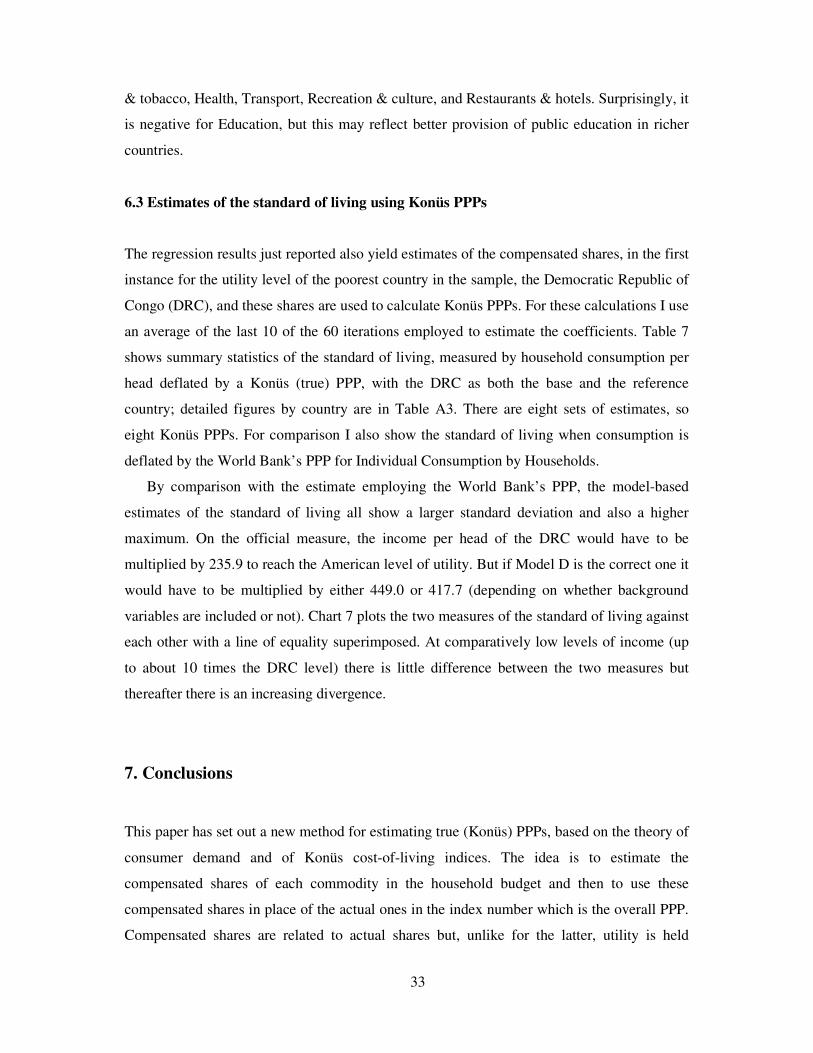
33
& tobacco, Health, Transport, Recreation & culture, and Restaurants & hotels. Surprisingly, it
is negative for Education, but this may reflect better provision of public education in richer
countries.
6.3 Estimates of the standard of living using Konüs PPPs
The regression results just reported also yield estimates of the compensated shares, in the first
instance for the utility level of the poorest country in the sample, the Democratic Republic of
Congo (DRC), and these shares are used to calculate Konüs PPPs. For these calculations I use
an average of the last 10 of the 60 iterations employed to estimate the coefficients. Table 7
shows summary statistics of the standard of living, measured by household consumption per
head deflated by a Konüs (true) PPP, with the DRC as both the base and the reference
country; detailed figures by country are in Table A3. There are eight sets of estimates, so
eight Konüs PPPs. For comparison I also show the standard of living when consumption is
deflated by the World Bank’s PPP for Individual Consumption by Households.
By comparison with the estimate employing the World Bank’s PPP, the model-based
estimates of the standard of living all show a larger standard deviation and also a higher
maximum. On the official measure, the income per head of the DRC would have to be
multiplied by 235.9 to reach the American level of utility. But if Model D is the correct one it
would have to be multiplied by either 449.0 or 417.7 (depending on whether background
variables are included or not). Chart 7 plots the two measures of the standard of living against
each other with a line of equality superimposed. At comparatively low levels of income (up
to about 10 times the DRC level) there is little difference between the two measures but
thereafter there is an increasing divergence.
7. Conclusions
This paper has set out a new method for estimating true (Konüs) PPPs, based on the theory of
consumer demand and of Konüs cost-of-living indices. The idea is to estimate the
compensated shares of each commodity in the household budget and then to use these
compensated shares in place of the actual ones in the index number which is the overall PPP.
Compensated shares are related to actual shares but, unlike for the latter, utility is held

34
constant at some given level while prices can vary. To derive compensated shares from actual
ones we need to estimate the semi-elasticities of the budget shares with respect to
expenditure. This has been done by fitting a model of consumer demand econometrically
using the same data as underlies the World Bank’s overall PPPs, namely PPPs at the Basic
Heading level together with the corresponding expenditures. The econometric analysis has
taken account of within-country as well as cross-country income inequality, and also of
background variables which may influence spending patterns independently of prices and
income.
The aim of the exercise has not been to test the theory of consumer demand, which is best
done at the individual level, but rather to use it to obtain better estimates of the standard of
living across the world. Nonetheless, some interesting facts have emerged about the structure
of demand at the level of the 100 Basic Headings within Household Consumption. On
average we have been able to explain about 59% of the variation in budget shares across our
141 countries using prices, income (expenditure), and background variables such as religion,
culture, and climate as explanatory factors. Strong support for non-homotheticity has also
emerged.
Household Consumption deflated by these new, Konüs PPPs answers the question: by
how much must the average expenditure per head of poor country A be increased to enable
the typical inhabitant of A to enjoy the same utility level as the typical inhabitant of rich
country B? These new estimates of the standard of living show a much greater dispersion
across countries than when consumption is deflated by the World Bank’s PPPs: the standard
of living in the poorest countries is now only about half the level estimated using the World
Bank’s PPPs.
Finally, it is important to distinguish between the standard of living and productivity. If
this paper is correct that the standard of living in the poorest countries is only half the level as
conventionally measured, this does not necessarily mean that productivity is equally low
(though it might be). So it does not necessarily follow that the poorest countries will take
twice as long to catch up. Measuring productivity correctly raises similar issues to measuring
the standard of living. For the latter, the issue is whether tastes are homothetic, for the former
whether there are economies of scale in production. These are different issues though
conceptually they can be resolved in a similar way (Oulton, 2009). The data underlying the
ICP come from the expenditure side of the national accounts. To study productivity we need
to employ a comparably detailed dataset from the output side.

35
Table 1
Real household consumption per head for 146a countries:
effect of different deflators, summary statistics (poorest country = 1)
Deflator
Statistic Exchange rate
World Bank PPP
Multilat-eral (EKS
Fisher)
Bilateral PPP (own
weights)
Bilateral PPP (U.S.
weights)
Minimum 1.0 1.0 1.0 1.0 1.0
Maximum 397.4 235.9 223.9 190.6 247.8
Mean 70.7 50.3 49.9 46.6 49.6
S.D. 101.0 54.5 53.5 46.6 56.4
a. 145 countries when exchange rate used (Zimbabwe is missing).
Notes Poorest country is Democratic Republic of Congo (DRC), richest is U.S. Household
consumption is sum of Basic Headings 1-102, 104 & 105: see Appendix Table A1 for the list
of Basic Headings. “World Bank PPP” is the World Bank’s PPP for Individual Consumption
by Households. The other PPPs are my own. The bilateral PPP with own weights uses each
country’s expenditure shares to weight the individual PPPs.
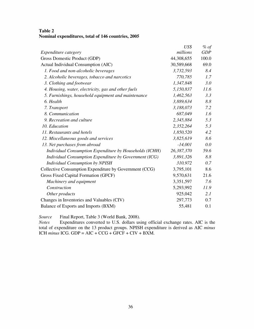
36
Table 2
Nominal expenditures, total of 146 countries, 2005
Expenditure category US$
millions % of GDP
Gross Domestic Product (GDP) 44,308,655 100.0
Actual Individual Consumption (AIC) 30,589,668 69.0
1. Food and non-alcoholic beverages 3,732,593 8.4
2. Alcoholic beverages, tobacco and narcotics 770,785 1.7
3. Clothing and footwear 1,347,848 3.0
4. Housing, water, electricity, gas and other fuels 5,150,837 11.6
5. Furnishings, household equipment and maintenance 1,462,563 3.3
6. Health 3,889,634 8.8
7. Transport 3,188,073 7.2
8. Communication 687,049 1.6
9. Recreation and culture 2,345,884 5.3
10. Education 2,352,264 5.3
11. Restaurants and hotels 1,850,520 4.2
12. Miscellaneous goods and services 3,825,619 8.6
13. Net purchases from abroad -14,001 0.0
Individual Consumption Expenditure by Households (ICHH) 26,387,370 59.6
Individual Consumption Expenditure by Government (ICG) 3,891,326 8.8
Individual Consumption by NPISH 310,972 0.7
Collective Consumption Expenditure by Government (CCG) 3,795,101 8.6
Gross Fixed Capital Formation (GFCF) 9,570,631 21.6
Machinery and equipment 3,351,597 7.6
Construction 5,293,992 11.9
Other products 925,042 2.1
Changes in Inventories and Valuables (CIV) 297,773 0.7
Balance of Exports and Imports (BXM) 55,481 0.1
Source Final Report, Table 3 (World Bank, 2008).
Notes Expenditures converted to U.S. dollars using official exchange rates. AIC is the
total of expenditure on the 13 product groups. NPISH expenditure is derived as AIC minus ICH minus ICG. GDP = AIC + CCG + GFCF + CIV + BXM.

37
Table 3
ICP regions
ICP region Number of countries Population (millions) Africa 47 756
Asia/Pacific 23 3,346
West Asia 11 176
South America 10 366
CIS 10 247
OECD-Eurostat 45 1,238
Total 146 6,128

38
Table 4
Number of countries reporting zero expenditure for selected Basic Headings,
in descending order
BH Number Basic Heading
Number of countries
98 Prostitution 81
76 Combined passenger transport 53
106 Net purchases abroad 44
103 FISIM 42
72 Passenger transport by railway 22
90 Games of chance 20
92 Package holidays 20
75 Passenger transport by sea and inland waterway 16
104 Other financial services n.e.c. 15
87 Veterinary and other services for pets 14
7 Pork 11
86 Gardens and pets 10
31 Wine 9
42 Miscellaneous services relating to the dwelling 9
77 Other purchased transport services 9
101 Social protection 9
30 Spirits 8
32 Beer 7
48 Repair of furniture, furnishings and floor coverings 7
54 Major tools and equipment 7
83
Repair of audio-visual, photographic and information
processing equipment 7
105 Other services n.e.c. 7
Source Unpublished World Bank spreadsheet.

39
Table 5
The 11 countries recording the largest number of zero expenditures
for Basic Headings within Household Consumption (BH 1-105).
Country ICP region Number
of zeros
Comoros Africa 42
Angola Africa 26
Djibouti Africa 21
Tanzania Africa 19
Maldives Asia/Pacific 18
Zambia Africa 13
Bhutan Asia/Pacific 13
Lao PDR Asia/Pacific 11
Ethiopia Africa 10
Rwanda Africa 10
Bangladesh Asia/Pacific 10
TOTAL 193
Source Unpublished World Bank spreadsheet.
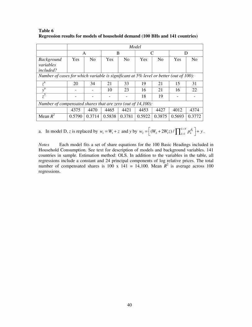
40
Table 6
Regression results for models of household demand (100 BHs and 141 countries)
Model
A B C D
Background variables included?
Yes No Yes No Yes No Yes No
Number of cases for which variable is significant at 5% level or better (out of 100):
za 20 34 21 33 19 21 15 31
ya - - 10 23 16 21 16 22
z3 - - - - 18 19 - -
Number of compensated shares that are zero (out of 14,100):
4375 4470 4465 4421 4453 4427 4012 4374
Mean R2 0.5790 0.3714 0.5838 0.3781 0.5922 0.3875 0.5693 0.3772
a. In model D, z is replaced by 1 1w W z= + and y by 2 2 1 1( 2 ) / k
k N
kkw W W z p yβ=
= = + + ∏ .
Notes Each model fits a set of share equations for the 100 Basic Headings included in
Household Consumption. See text for description of models and background variables. 141
countries in sample. Estimation method: OLS. In addition to the variables in the table, all
regressions include a constant and 24 principal components of log relative prices. The total
number of compensated shares is 100 x 141 = 14,100. Mean R2 is average across 100
regressions.

41
Table 7
Mean values of estimated coefficients on expenditure variables, by product group
Model B Model D
Product group z y w1 w2
1 Food & non-alcoholic drink -0.1653 -0.000002 -0.1800 0.000039
2 Alcohol & tobacco 0.2347 -0.000193 0.2052 -0.000130
3 Clothing & footwear -0.0409 0.000060 0.0100 0.000243
4 Housing, water, electricity & fuels -0.1109 0.001105 -0.1033 0.000241
5 Furniture & household equipment 0.0538 -0.000011 0.0460 0.000014
6 Health 0.1368 0.000135 0.1525 -0.000115
7 Transport 0.1903 -0.000473 0.1553 0.000118
8 Communication -0.1360 -0.000597 -0.1106 -0.000241
9 Recreation & culture 0.1271 0.000037 0.1234 0.000006
10 Education -0.6884 -0.002391 -0.4167 -0.001660
11 Restaurants & hotels 0.1920 0.000708 0.2548 -0.000046
12 Miscellaneous 0.0736 -0.000113 0.0919 -0.000206
Notes Background variables included. For definitions of product groups, see Table A1 in
the Data Appendix.
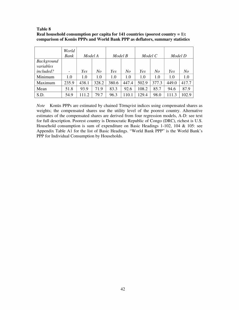
42
Table 8
Real household consumption per capita for 141 countries (poorest country = 1):
comparison of Konüs PPPs and World Bank PPP as deflators, summary statistics
World Bank Model A Model B Model C Model D
Background variables included? - Yes No Yes No Yes No Yes No
Minimum 1.0 1.0 1.0 1.0 1.0 1.0 1.0 1.0 1.0
Maximum 235.9 438.1 328.2 380.6 447.4 502.9 377.3 449.0 417.7
Mean 51.8 93.9 71.9 83.3 92.6 108.2 85.7 94.6 87.9
S.D. 54.9 111.2 79.7 96.3 110.1 129.4 98.0 111.3 102.9
Note Konüs PPPs are estimated by chained Törnqvist indices using compensated shares as
weights; the compensated shares use the utility level of the poorest country. Alternative
estimates of the compensated shares are derived from four regression models, A-D: see text
for full description. Poorest country is Democratic Republic of Congo (DRC), richest is U.S.
Household consumption is sum of expenditure on Basic Headings 1-102, 104 & 105: see
Appendix Table A1 for the list of Basic Headings. “World Bank PPP” is the World Bank’s
PPP for Individual Consumption by Households.
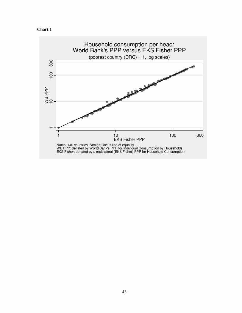
43
Chart 1
110
100
30
0W
B P
PP
1 10 100 300EKS Fisher PPP
Notes: 146 countries. Straight line is line of equality.WB PPP: deflated by World Bank's PPP for Individual Consumption by Households;EKS Fisher: deflated by a multilateral (EKS Fisher) PPP for Household Consumption
(poorest country (DRC) = 1, log scales)
Household consumption per head:World Bank's PPP versus EKS Fisher PPP

44
Chart 2
210
50
100
Infa
nt m
ort
alit
y (
de
ath
s p
er
1000 liv
e b
irth
s)
1 10 100 200Real household consumption per head (DRC = 1)
Notes: 146 countries. Household consumption deflated by EKS Fisher PPP.
(log scales)
Infant mortality versus household consumption per head

45
Chart 3
40
50
60
70
80
90
Life e
xpecta
ncy
(ye
ars
)
1 10 100 200Real household consumption per head (DRC = 1)
Notes: 144 countries. Household consumption deflated by EKS Fisher PPP.
(log scales)
Life expectancy versus household consumption per head

46
Chart 4
35
45
55
65
75
Gin
i co
effic
ien
t (%
)
1 10 100 200Real household consumption per head (DRC = 1)
Notes: 126 countries. Household consumption deflated by EKS Fisher PPP.
(log scale for household consumption)
Inequality (Gini) versus household consumption per head

47
Chart 5
01
02
03
04
0F
req
ue
ncy
-1 -.5 0 .5 1
Distribution of estimated coefficients on W1:Model D, background variables included

48
Chart 6
020
40
60
Fre
quen
cy
-.004 -.002 0 .002
Distribution of estimated coefficients on W2:Model D, background variables included

49
Chart 7
110
25
0600
Kon
üs
1 10 100 200 300Conventional
Notes: 141 countries. Straight line is line of equality.Conventional: deflated by EKS Törnqvist PPP;Konüs: deflated by Konüs PPP, estimated by model D with background variables included.
(poorest country = 1, log scales)
Household consumption per head:conventional versus Konüs, with poorest country as base

50
Data Appendix
A.1 The World Bank dataset
I received a spreadsheet on 3rd
July 2008 from the World Bank entitled “Final detailed
results-Researchers.xls”, which contains some of the unpublished data which underlies their
published results. This dataset consisted of expenditures and corresponding PPPs for each of
the 129 Basic Headings which make up GDP; the expenditures and PPPs were for each of the
146 countries that were eventually included in the ICP. That is, there were in all (146 x 129
= ) 18,834 PPPs and the same number of expenditures, with no missing values. The
expenditures are expressed in local currency units and the PPPs as local currency units per
U.S. dollar. In addition, the spreadsheet included population and official exchange rates.
Table A1 lists the Basic Headings (names and codes) and the product groups of the data that I
was sent. Note that this list does not correspond exactly to the official classification scheme
(World Bank, 2008, Appendix C) since some Basic Headings within Individual Consumption
by Government were omitted and expenditures on them distributed to other Basic Headings
within Individual Consumption by Households: see section 5.1 for details. Table A2 lists all
the 146 countries that were eventually included in the 2005 ICP, ordered alphabetically
within each ICP region. The names are the official ones, which are not always the more
familiar ones. Thus “Congo, Dem. Rep.” is the Democratic Republic of Congo (DRC). Table
A2 also gives Household Consumption (see section 5.2 for the exact definition) as measured
using five different deflators: the official exchange rate, the World Bank’s PPP for Individual
Consumption by Households, and three deflators that I estimated myself: a multilateral EKS
Fisher PPP, a bilateral PPP constructed using each country’s expenditure weights, and a
bilateral PPP using U.S. expenditure weights. The reference country is the DRC. Table A3
lists the 141 countries included in the analysis of consumer demand (ie omitting Angola,
Comoros, Djibouti, Tanzania and Maldives) and shows Household Consumption deflated by
Konüs PPPs estimated eight different ways; that is, from Models A-D each estimated with
and without the background variables. The DRC is both base and reference country here.
51
A.2 Background variables
Two criteria were employed for selecting socio-economic variables: (a) relevance and (b)
availability for all (or almost all) the 146 (later 141) countries. The chosen variables fell into
the following broad groups:
1. Climate (5 variables)
a. Rainfall (centimetres per year, in logs)
b. Proportion of frost days (number of frost days ÷ 365)
c. Minimum temperature (degrees Celsius)
d. Maximum temperature (degrees Celsius)
e. Distance from the equator (degrees latitude North or South of the equator ÷
90)
Sources: The first four variables come from the TYN CY 1.1 dataset and were downloaded
from the Tyndall Centre at the University of East Anglia on October 30 2008.
(http://www.cru.uea.ac.uk/~timm/cty/obs/TYN_CY_1_1_text.html). These measures are
area-weighted averages for each country (30 year averages, using 1 degree squares): see
Mitchell et al. (2003). (Population-weighted averages would have been more suitable for my
purposes but these do not seem to be available). Distance from the equator comes from the
unpublished appendix to Hall and Jones (1999), downloaded from http://elsa.berkeley.edu/
~chad/HallJones400.asc on 14th December 2008.
2. Religion (4 variables)
a. Proportion of population that is Christian (ratio)
b. Proportion of population that is Muslim (ratio)
c. Proportion of population that is Buddhist (ratio)
d. Proportion of population that is Hindu (ratio)
Source: Barro’s dataset on religious adherence, http://www.economics.harvard.edu/faculty/
barro/files/religion%20adherence%20data.xls, downloaded from his website on 7th
November 2008. The proportion Christian is the sum of the proportions Catholic, Protestant,
Orthodox and Other Christian. These four variables sum to less than one: the omitted
categories are Jewish, Eastern religions, Other religions and Non-religious.

52
3. Hegemony and culture (7 dummy variables)
a. U.S. hegemony (= 1 if subject to U.S. hegemony, 0 otherwise: 11 Latin
American countries including Mexico plus Liberia and the Philippines)
b. Russian hegemony (= 1 if subject to Russian hegemony, 0 otherwise: the 18
countries which were either under the domination of the Soviet Union or are
the successor states to the Soviet Union).
c. U.K. hegemony (= 1 if subject to U.K. hegemony, 0 otherwise: 39 countries)
d. French hegemony (= 1 if subject to French hegemony, 0 otherwise: 25
countries)
e. Belgian hegemony (= 1 if subject to Belgian hegemony, 0 otherwise: 3
countries)
f. Portuguese hegemony (= 1 if subject to Portuguese hegemony, 0 otherwise: 8
countries)
g. Arab culture (= 1 if a country is predominantly Arab in language and ethnicity,
0 otherwise: 15 countries)
Sources: General knowledge, judgement, and the CIA World Fact Book.
4. Health (3 variables)
a. Life expectancy at birth (years)
b. Infant mortality (rate per thousand live births)
c. Public expenditure on health as a percentage of GDP
Source: World Development Indicators (WDI). These and other data were downloaded from
the World Bank’s World Development Indicator (WDI) database (http://go.worldbank.org/
6HAYAHG8H0) on 12 August 2008: Life expectancy for females is higher than for males in
all but three of our 146 countries, but the gap is fairly small, except for Russia (an amazing
13.5 years), the CIS and the Baltic states.
5. Education (3 variables)
a. Proportion of population over 25 with at most primary education (ratio)
b. Proportion of population over 25 with at most secondary education (ratio)
c. Proportion of population over 25 with higher education (ratio)
d. Proportion of population over 25 with no schooling (ratio); omitted in
regressions
53
Source: Cohen and Soto (2007). The Cohen-Soto educational database was downloaded from
http://www.oecd.org/dataoecd/33/13/2669521.xls on 10th January 2009. The Cohen-Soto
data were available for only 81 countries out of the 146 in our sample. An additional 24
countries, making 105 in all, were extrapolated from World Development Indicators (WDI).
The procedure was to regress the Cohen-Soto measures on similar WDI ones, then use the
regression to predict a Cohen-Soto measure for the 24 countries where WDI was known but
Cohen-Soto was missing.
6. Urbanisation (1 variable)
a. Urban population as percentage of total. Source: WDI.
7. Policy (1 variable)
a. Openness: 100 x (exports plus imports)/GDP, adjusted for population size.
Source: Penn World Table 6.2. The size adjustment consisted of regressing the PWT
openness variable on log population, log population squared, and log population cubed, then
taking the residual from this regression as the measure of size-adjusted openness. In practice
the size adjustment makes little difference.
8. Demography (2 variables)
a. Proportion of population aged under 15 (ratio)
b. Proportion of population aged over 64 (ratio)
c. Source: World Development Indicators. The 2005 value was chosen where
available, otherwise the year closest to 2005. The missing variable is the
proportion of population aged 15-64.
9. Inequality (2 variables)
a. 1 ln( )W G I= −
b. 2
2 2 ln( ) [ln( )]W J I G G= − +
Here 10G = , 10
1ln
g
g ggI w w
=
== −∑ , and 2
1(ln )
g G
g ggJ w w
=
==∑ where gw is the share of the
gth decile in aggregate income; I is the share-weighted average of log shares (entropy) and J
is a kind of second moment. Decile shares were used to calculate I and J since these were the
most detailed available. Source: UNU-WIDER World Income Inequality Database, version
2.0c (May 2008), downloaded from http://www.wider.unu.edu/research/Database/
54
en_GB/database/ on 13 August 2008; version 2b is described in UNU-WIDER (no date; c.
2008). For 114 countries, data exist for all decile shares. For a further 9 countries, there is
data for the first and 10th
decile shares. The missing decile shares for these 9 countries were
interpolated by regressing the share of decile 2 (3,4,...,9) on deciles shares 1 and 10 plus the
ICP region dummies for 114 countries and using this regression to predict decile shares 2-9
for the other 9 countries. This still left the problem of estimating the decile shares for the
remaining 23 countries where they are completely missing. These shares were extrapolated
by means of a regression approach. I regressed each decile share in turn on a battery of
variables and used the regression equation to predict values of the decile shares for the 23
missing countries. The battery of variables consisted of the Gini coefficient (when available),
public health expenditure as a percentage of GDP, infant mortality (these three variables from
the WDI), the demographic and climate variables (see above), the ICP region dummies, and a
“mining” dummy, equal to 1 if I judged a country’s economy to be dominated by extractive
industries (oil, diamonds or tin; 17 countries fell into this category). One country, Macao,
could not be extrapolated by this method because some or all of the background variables
were missing. This was filled in by using the results for Hong Kong.
10. World Bank ICP region (5 dummy variables)
A set of 6 dummy variables, one for each ICP “region”, each taking the value 1 if a country
fell into that region, 0 otherwise. The regions are: Africa, Asia/Pacific, West Asia, South
America, Commonwealth of Independent States (CIS), and OECD-Eurostat; the latter is
omitted in the regressions. These dummy variables correspond only roughly to geography.
For example, Mexico is in the OECD-Eurostat region, not in the South American one, and
OECD-Eurostat includes countries from North America (eg the U.S.), the Middle East
(Israel) and East Asia (Japan and Korea). But the ICP regions did their work independently of
each other (though under World Bank supervision and coordination), so it is possible that
there are methodological differences between them which the region dummies will pick up.
Thus there are in all 30 “background” variables which I have been able to find and which
might arguably influence spending patterns independently of prices and incomes. This
number rises to 33 variables if the three educational variables (available even after some
extrapolation for only 105 countries) are also included.

55
Table A1
Basic Headings and product groups in the 2005 ICP
Basic Heading number
Basic Heading
code Basic Heading name
Product group
number
Product group code
Product group name
1 1101111 Rice
1 110100
Food and
nonalcoholic
beverages
[29 Basic
Headings]
2 1101112 Other cereals and flour
3 1101113 Bread
4 1101114 Other bakery products
5 1101115 Pasta products
6 1101121 Beef and veal
7 1101122 Pork
8 1101123 Lamb, mutton and goat
9 1101124 Poultry
10 1101125 Other meats and preparations
11 1101131 Fresh or frozen fish and seafood
12 1101132 Preserved fish and seafood
13 1101141 Fresh milk
14 1101142 Preserved milk and milk products
15 1101143 Cheese
16 1101144 Eggs and egg-based products
17 1101151 Butter and margarine
18 1101153 Other edible oils and fats
19 1101161 Fresh or chilled fruit
20 1101162 Frozen, preserved or processed fruits
21 1101171 Fresh or chilled vegetables
22 1101172 Fresh or chilled potatoes
23 1101173 Frozen or preserved vegetables
24 1101181 Sugar
25 1101182 Jams, marmalades and honey
26 1101183 Confectionery, chocolate and ice cream
27 110119 Food products n.e.c.
28 110121 Coffee, tea and cocoa
29 110122 Mineral waters, soft drinks,
30 1102111 Spirits
2 110200
Alcoholic
beverages,
tobacco, and
narcotics
[4 Basic
Headings]
31 1102121 Wine
32 1102131 Beer
33 110220 Tobacco
34 1103111 Clothing materials and accessories
3 110300
Clothing and
footwear
[5 Basic
Headings]
35 1103121 Garments
36 1103141 Cleaning and repair of clothing
37 1103211 Footwear
38 1103221 Repair and hire of footwear
39 110410 Actual and imputed rentals for housing
4 110400
Housing,
water,
electricity,
gas, and
other fuels
[7 Basic
Headings]
40 110430 Maintenance and repair of the dwelling
41 110440 Water supply and miscellaneous
services
relating to the dwelling
42 110442 Miscellaneous services relating to the
dwelling
43 110451 Electricity
44 110452 Gas
45 110453 Other fuels
46 110511 Furniture and furnishings
5 110500
Furniture,
household
equipment,
47 110512 Carpets and other floor coverings
48 110513 Repair of furniture, furnishings and

56
floor coverings and routine
maintenance
of the house
[13 Basic
Headings]
49 110520 Household textiles
50 110531 Major household appliances whether
electric or not
51 110532 Small electric household appliances
52 110533 Repair of household appliances
53 110540 Glassware, tableware and household
utensils
54 110551 Major tools and equipment
55 110552 Small tools and miscellaneous
accessories
56 110561 Non-durable household goods
57 1105621 Domestic services
58 1105622 Household services
59 110611 Pharmaceutical products
6 110600
Health
[7 Basic
Headings]
60 110612 Other medical products
61 110613 Therapeutical appliances and
equipment
62 110621 Medical Services
63 110622 Dental services
64 110623 Paramedical services
65 110630 Hospital services
66 110711 Motor cars
7 110700
Transport
[12 Basic
Headings]
67 110712 Motor cycles
68 110713 Bicycles
69 110722 Fuels and lubricants for personal
transport
equipment
70 110723 Maintenance and repair of personal
transport
equipment
71 110724 Other services in respect of personal
transport
equipment
72 110731 Passenger transport by railway
73 110732 Passenger transport by road
74 110733 Passenger transport by air
75 110734 Passenger transport by sea and inland
waterway
76 110735 Combined passenger transport
77 110736 Other purchased transport services
78 110810 Postal services
8 110800
Communicat
ion
[3 Basic
Headings]
79 110820 Telephone and telefax equipment
80 110830 Telephone and telefax services
81 110911 Audio-visual, photographic and
information
processing equipment
9 110900
Recreation
and culture
[12 Basic
Headings]
82 110914 Recording media
83 110915 Repair of audio-visual, photographic
and
information-processing equipment
84 110921 Major durables for outdoor and indoor
recreation
85 110931 Other recreational items and equipment
86 110933 Gardens and pets
87 110935 Veterinary and other services for pets
88 110941 Recreational and sporting services
89 110942 Cultural services

57
90 110943 Games of chance
91 110950 Newspapers, books and stationery
92 110960 Package holidays
93 111000 Education 10 111000 Education
94 111110 Catering services
11 111100
Restaurants
and hotels
[2 Basic
Headings]
95 111120 Accommodation services
96 111211 Hairdressing salons and personal
grooming
Establishments
12 111200
Miscellaneo
us goods
and services
[10 Basic
Headings]
97 111212 Appliances, articles and products for
personal care
98 111220 Prostitution
99 111231 Jewellery, clocks and watches
100 111232 Other personal effects
101 111240 Social protection
102 111250 Insurance
103 111261 FISIM
104 111262 Other financial services n.e.c
105 111270 Other services n.e.c.
106 111300 Net purchases abroad
13 111300
Balance of
expenditures
of residents
abroad
and
expenditures
of
nonresidents
on the
economic
territory
107 130221 Compensation of employees
14
Individual
consumption
expenditure
by
government:
Health
[5 Basic
Headings]
108 130222 Intermediate consumption
109 130223 Gross operating surplus
110 130224 Net taxes on production
111 130225 Receipts from sales
112 130421 Compensation of employees
15
Individual
consumption
expenditure
by
government:
Education
[5 Basic
Headings]
113 130422 Intermediate consumption
114 130423 Gross operating surplus
115 130424 Net taxes on production
116 130425 Receipts from sales
117 140111 Compensation of employees
16
Collective
consumption
expenditure
by
government
[5 Basic
Headings]
118 140112 Intermediate consumption
119 140113 Gross operating surplus
120 140114 Net taxes on production
121 140115 Receipts from sales
122 150110 Metal products and equipment
17
Expenditure
on gross
fixed
capital
formation
123 150120 Transport equipment
124 150210 Residential buildings
125 150220 Non-residential buildings
126 150230 Civil engineering works

58
127 150300 Other products [6 Basic
Headings]
128 160000 Change in inventories and valuables
18
Changes in
inventories
and
valuables
129 180000 Balance of exports and imports
19
Balance of
exports
and imports
GDP Total
Source World Bank. This listing is shorter than the one in World Bank (2008, Appendix C) since some
BHs within Individual Consumption Expenditure by Government for which no expenditures or PPPs were
included in the unpublished World Bank spreadsheet have been omitted: see text for more detail.
Note The numbering of the Basic Headings and of the Product groups is my own; all other terms follow
World Bank usage.

59
Table A2
Real household consumption per head:
effect of different deflators (poorest country = 1.0)
Deflator
Country and ICP region Exchange
rate World
Bank PPP
Multilat-eral (EKS
Fisher)
Bilateral PPP (own weights)
Bilateral PPP (U.S. weights)
Africa
Angola 5.9 4.5 4.3 4.3 4.4
Benin 5.6 7.1 7.1 6.9 6.7
Botswana 19.4 19.6 19.1 19.9 18.3
Burkina Faso 3.8 5.5 5.1 4.8 4.6
Burundi 1.1 1.8 1.7 2.2 1.5
Cameroon 8.2 9.9 9.4 9.0 8.7
Cape Verde 22.3 16.9 16.1 16.6 15.9
Central African Republic 4.0 4.6 4.3 4.6 3.7
Chad 5.0 5.3 5.0 4.2 5.2
Comoros 6.8 6.1 5.6 6.3 5.4
Congo, Dem. Rep. 1.0 1.0 1.0 1.0 1.0
Congo, Rep. 6.5 6.1 6.0 5.8 6.1
Côte d'Ivoire 7.1 7.7 7.5 7.2 7.0
Djibouti 6.9 7.6 7.0 8.5 6.1
Equatorial Guinea 23.9 19.3 19.0 24.2 17.3
Ethiopia 1.5 3.2 2.8 2.6 2.4
Gabon 23.7 18.8 18.5 19.1 18.7
Gambia, The 2.0 3.6 3.6 6.6 3.0
Ghana 4.7 6.4 6.3 7.2 6.0
Guinea 2.6 4.2 4.3 6.1 3.5
Guinea-Bissau 2.3 2.9 2.7 3.0 2.4
Kenya 5.3 8.1 7.7 8.9 7.2
Lesotho 9.1 11.3 11.2 16.6 9.8
Liberia 1.3 1.7 1.7 3.0 1.3
Madagascar 2.9 5.0 4.9 6.8 4.1
Malawi 2.3 3.2 3.1 4.5 2.6
Mali 4.1 5.0 4.8 4.5 4.7
Mauritania 5.4 7.6 7.0 6.3 7.0
Mauritius 44.8 49.7 43.9 39.4 43.1
Morocco 15.3 16.4 15.0 13.1 14.5
Mozambique 2.9 3.9 3.5 3.0 3.1
Namibia 21.3 17.9 17.3 17.7 17.2
Niger 2.4 3.2 3.0 2.8 2.7
Nigeria 7.3 8.2 8.3 8.1 8.9

60
Rwanda 2.5 4.0 3.6 4.3 2.9
Sao Tomé and Principe 8.7 9.6 9.0 9.9 8.2
Senegal 7.6 9.0 8.6 7.8 8.4
Sierra Leone 3.4 4.7 4.4 5.3 4.1
South Africa 40.6 37.7 36.0 35.7 34.3
Sudan 9.5 12.6 12.0 12.2 12.1
Swaziland 18.0 20.5 19.5 25.9 17.9
Tanzania 3.5 5.5 5.0 3.9 4.8
Togo 4.9 6.1 6.0 6.2 5.6
Tunisia 24.5 30.3 27.6 25.8 26.1
Uganda 3.2 5.2 5.0 6.3 4.3
Zambia 5.2 5.5 5.4 6.5 4.7
Zimbabwe n.a. 2.6 2.3 2.4 2.0
Asia/Pacific
Bangladesh 4.1 7.0 7.0 7.7 6.1
Bhutan 7.4 11.9 11.6 9.7 10.4
Brunei Darussalam 78.1 80.1 77.8 72.8 80.8
Cambodia 4.5 7.7 7.8 9.5 6.6
China 8.4 11.3 11.2 11.3 11.2
Fiji 33.3 24.2 23.5 21.9 23.0
Hong Kong, China 180.5 129.4 129.2 120.4 135.3
India 5.1 9.6 9.6 10.2 7.8
Indonesia 10.3 16.0 15.5 15.5 14.4
Iran, Islamic Rep. 20.2 44.5 45.8 56.2 38.5
Lao PDR 3.7 7.0 6.9 7.4 5.7
Macao, China 85.9 71.4 71.3 67.2 75.1
Malaysia 27.7 33.2 32.1 27.4 32.2
Maldives 14.5 12.7 12.8 18.7 11.5
Mongolia 6.3 9.7 9.5 10.6 8.8
Nepal 3.4 6.1 6.0 6.2 4.5
Pakistan 7.4 14.2 14.2 16.4 12.1
Philippines 9.7 14.8 15.0 16.7 13.7
Singapore 140.8 106.1 103.2 101.8 104.0
Sri Lanka 10.8 18.1 17.8 17.2 15.5
Taiwan, China 118.3 112.2 113.3 125.6 121.9
Thailand 18.9 29.0 28.2 24.8 27.4
Vietnam 4.6 8.3 8.4 12.2 6.3
West Asia
Bahrain 93.6 74.2 72.6 68.1 62.0
Egypt, Arab Rep. 12.7 24.2 23.1 23.0 22.7
Iraq 6.9 10.6 10.4 9.6 9.9
Jordan 24.5 23.7 25.2 24.9 24.4

61
Kuwait 132.4 91.5 95.7 98.7 80.4
Lebanon 61.0 55.5 60.6 62.6 63.1
Oman 51.0 44.6 46.7 43.2 43.1
Qatar 113.5 75.7 73.0 94.5 51.2
Saudi Arabia 45.1 38.9 40.6 37.1 38.7
Syrian Arab Republic 13.0 18.4 18.6 18.3 18.9
Yemen, Rep. 6.3 8.8 9.2 8.9 9.2
South America
Argentina 36.0 51.5 48.8 46.1 46.5
Bolivia 8.1 17.0 15.7 17.2 13.5
Brazil 34.1 35.2 32.7 32.0 33.1
Chile 51.8 50.0 46.6 43.3 48.0
Colombia 22.0 28.5 26.5 27.4 25.8
Ecuador 22.2 29.6 27.0 24.8 27.1
Paraguay 11.6 22.5 21.2 20.7 18.5
Peru 23.4 31.2 28.5 29.4 26.9
Uruguay 44.8 47.8 44.8 42.7 42.9
Venezuela, RB 31.3 34.9 32.6 30.3 33.4
CIS
Armenia 14.1 21.9 26.1 32.0 19.9
Azerbaijan 9.1 16.4 18.4 18.7 14.3
Belarus 19.9 37.7 42.5 42.2 34.1
Georgia 12.4 19.2 23.2 31.5 17.7
Kazakhstan 23.7 32.4 38.8 60.8 31.0
Kyrgyz Republic 5.1 10.8 13.2 18.1 8.5
Moldova 9.5 16.6 21.3 28.0 14.7
Russian Federation 33.0 46.5 50.8 45.9 45.0
Tajikistan 3.1 7.0 9.8 13.3 5.1
Ukraine 13.7 27.3 31.3 35.5 23.2
OECD-Eurostat
Albania 25.1 28.0 28.8 27.3 26.8
Australia 245.0 146.7 146.4 125.4 152.6
Austria 294.0 176.3 172.2 149.0 181.2
Belgium 261.4 150.1 147.1 132.4 154.8
Bosnia and Herzegovina 35.4 42.6 42.9 39.4 39.2
Bulgaria 33.0 46.7 48.0 48.2 42.5
Canada 246.8 158.2 156.1 131.6 165.7
Croatia 80.4 71.5 71.7 64.6 70.1
Cyprus 217.3 148.2 149.4 124.5 148.1
Czech Republic 85.0 89.4 90.3 88.0 86.8
Denmark 322.5 141.8 139.6 120.5 141.5
Estonia 77.0 73.2 75.7 66.8 75.3

62
Finland 259.6 128.3 128.1 111.4 130.4
France 269.4 153.0 152.9 131.7 159.9
Germany 267.6 157.0 152.5 135.8 161.3
Greece 197.0 136.6 134.7 115.4 137.2
Hungary 80.6 78.0 80.6 72.2 75.1
Iceland 397.4 160.3 159.0 132.1 163.3
Ireland 287.4 140.8 140.3 118.1 148.6
Israel 138.4 101.9 102.3 93.7 100.3
Italy 235.1 137.9 135.0 113.0 136.9
Japan 275.8 141.9 136.8 143.8 153.0
Korea, Rep. 105.6 82.1 77.8 83.3 81.6
Latvia 53.9 57.6 61.3 57.6 58.2
Lithuania 62.7 70.1 74.4 62.7 69.0
Luxembourg 367.1 217.7 204.7 176.7 212.7
Macedonia, FYR 26.8 37.5 38.8 37.5 33.9
Malta 137.1 118.6 118.0 97.2 115.8
Mexico 62.6 59.5 60.7 59.2 55.7
Montenegro 31.6 33.7 34.9 33.2 32.6
Netherlands 269.3 158.0 154.4 141.1 162.3
New Zealand 214.5 127.0 127.3 109.4 134.9
Norway 358.5 157.2 154.8 136.6 160.3
Poland 63.5 63.8 68.1 66.3 61.9
Portugal 152.3 109.8 108.0 90.2 107.4
Romania 39.8 44.9 45.6 43.0 42.7
Serbia 31.9 40.7 41.9 41.5 37.3
Slovak Republic 65.2 71.7 74.6 75.3 68.3
Slovenia 127.7 103.5 102.6 85.9 104.4
Spain 203.6 135.8 135.5 112.4 137.9
Sweden 270.4 140.8 137.1 124.2 140.4
Switzerland 368.9 164.6 160.8 146.8 178.3
Turkey 42.4 38.2 38.3 38.3 33.8
United Kingdom 303.9 169.0 170.4 139.3 173.6
United States 353.6 235.9 223.9 190.6 247.8
Notes Countries are ordered alphabetically within the six ICP regions. Poorest country is Democratic
Republic of Congo (DRC), richest is U.S. Household consumption is sum of Basic Headings 1-102, 104 & 105:
see Appendix Table A1 for the list of Basic Headings. “World Bank PPP” is the World Bank’s PPP for
Individual Consumption by Households. The other PPPs are my own. The bilateral PPP with own weights uses
each country’s expenditure shares in turn to weight the individual PPPs. The bilateral PPP with U.S. weights
uses U.S. expenditure shares to weight each country’s individual PPPs.

63
Table A3
Real household consumption per head in 141 countries:
deflation by Konüs PPPs (poorest country = 1.0)
Model
A B C D
Background variables included?
Country and ICP region Yes No Yes No Yes No Yes No
Africa
Benin 8.0 7.7 7.8 7.8 8.2 8.1 7.8 7.6
Botswana 26.0 26.3 26.0 26.2 28.8 24.2 25.8 25.3
Burkina Faso 5.6 5.5 5.4 5.6 5.7 5.8 5.3 5.5
Burundi 1.7 1.7 1.7 1.7 1.7 1.7 1.7 1.7
Cameroon 11.9 11.6 11.2 11.9 11.6 12.3 11.3 10.5
Cape Verde 20.1 19.4 20.7 19.4 22.4 18.8 20.2 18.1
Central African Republic 4.5 4.6 4.5 4.7 4.5 4.7 4.4 4.7
Chad 5.9 5.8 5.8 5.9 5.9 6.1 5.7 5.7
Congo, Dem. Rep. 1.0 1.0 1.0 1.0 1.0 1.0 1.0 1.0
Congo, Rep. 6.7 6.4 6.5 6.5 6.6 6.6 6.5 6.3
Côte d'Ivoire 8.9 8.1 8.6 8.3 9.0 9.0 8.5 8.1
Equatorial Guinea 21.9 22.1 22.3 22.8 24.9 21.1 22.1 21.3
Ethiopia 2.7 2.8 2.7 2.8 2.7 2.7 2.7 2.8
Gabon 22.8 22.1 23.2 22.7 25.7 21.0 22.9 21.6
Gambia, The 3.2 3.3 3.2 3.2 3.2 3.2 3.3 3.3
Ghana 6.8 6.9 6.6 7.1 6.8 7.0 6.6 6.8
Guinea 4.1 4.1 4.1 4.2 4.2 4.1 4.1 4.2
Guinea-Bissau 2.6 2.6 2.6 2.6 2.6 2.6 2.6 2.6
Kenya 9.4 8.4 9.1 8.7 9.4 9.5 8.8 8.1
Lesotho 12.7 13.1 12.0 13.5 12.4 14.0 12.1 11.8
Liberia 1.5 1.5 1.5 1.5 1.5 1.5 1.5 1.5
Madagascar 5.1 5.0 4.8 5.1 4.9 5.0 4.8 4.8
Malawi 3.1 3.2 3.1 3.2 3.1 3.2 3.1 3.3
Mali 5.0 4.9 4.9 5.0 5.0 5.1 4.9 4.9
Mauritania 8.2 7.7 7.9 7.9 8.3 8.3 7.9 7.7
Mauritius 81.4 61.4 73.2 73.3 91.9 68.5 82.7 72.7
Morocco 19.0 19.3 17.6 19.6 18.5 17.8 17.8 18.3
Mozambique 3.9 3.9 3.9 3.9 3.8 3.9 3.8 3.9
Namibia 20.1 20.7 20.3 21.7 22.3 20.4 20.4 20.4
Niger 3.2 3.3 3.2 3.2 3.2 3.2 3.3 3.3
Nigeria 9.8 9.0 8.9 9.3 9.3 9.8 8.7 8.1
Rwanda 3.8 3.8 3.8 3.8 3.8 3.8 3.7 3.8
Sao Tomé and Principe 11.1 10.5 10.6 10.8 10.9 11.3 10.7 9.6
Senegal 10.8 9.8 10.3 10.1 10.5 10.8 10.3 9.1

64
Sierra Leone 4.4 4.4 4.4 4.5 4.4 4.4 4.4 4.4
South Africa 59.1 51.9 55.3 56.3 62.7 58.3 65.5 61.7
Sudan 15.7 14.7 14.8 15.2 15.1 15.1 14.8 13.2
Swaziland 24.4 24.0 24.8 23.9 27.7 22.6 24.6 23.6
Togo 6.8 6.6 6.6 6.7 6.8 6.7 6.5 6.5
Tunisia 38.9 35.8 37.4 41.2 38.5 34.5 39.7 41.6
Uganda 5.0 5.0 5.0 5.0 5.0 4.9 5.0 4.8
Zambia 5.6 5.5 5.4 5.5 5.6 5.7 5.3 5.4
Zimbabwe 2.3 2.4 2.3 2.4 2.3 2.3 2.4 2.4
Asia/Pacific
Bangladesh 7.9 7.6 7.7 7.6 8.0 7.9 7.6 7.4
Bhutan 15.8 14.9 15.1 15.3 15.3 15.6 15.0 13.4
Brunei Darussalam 121.5 92.7 110.8 117.6 148.8 116.1 125.6 109.7
Cambodia 9.6 7.8 8.8 8.0 9.9 9.5 8.5 7.7
China 14.3 13.1 13.6 13.5 13.8 14.0 13.6 11.9
Fiji 31.0 30.0 30.2 31.9 35.6 30.9 31.3 29.9
Hong Kong, China 235.0 163.1 203.7 223.6 277.8 207.4 234.6 206.7
India 12.4 11.9 11.7 12.1 12.1 12.7 11.7 10.5
Indonesia 19.1 18.8 19.0 18.8 21.2 18.5 18.8 17.2
Iran, Islamic Rep. 64.8 51.9 58.7 56.5 72.6 56.7 68.6 61.6
Lao PDR 7.8 7.4 7.6 7.6 8.0 7.9 7.4 7.3
Macao, China 118.4 91.7 107.0 114.3 144.3 111.5 120.9 106.6
Malaysia 48.8 42.4 47.3 46.5 48.5 46.5 50.3 49.3
Mongolia 11.5 10.5 11.1 10.7 11.4 11.7 11.1 9.7
Nepal 7.0 6.7 6.8 6.8 7.1 7.0 6.7 6.7
Pakistan 17.6 17.4 16.8 17.4 17.1 17.4 16.6 15.5
Philippines 18.3 17.0 17.4 17.3 19.6 17.8 17.3 15.3
Singapore 185.5 136.4 159.1 178.9 218.2 175.7 183.4 168.8
Sri Lanka 22.5 25.0 22.8 24.9 25.5 22.9 22.4 22.0
Taiwan, China 199.9 137.0 172.2 187.2 235.9 175.9 197.8 170.0
Thailand 42.5 38.1 41.2 41.2 42.9 41.4 42.6 40.1
Vietnam 9.9 8.9 9.9 9.1 10.3 9.9 9.4 8.1
West Asia
Bahrain 132.0 104.1 118.5 134.8 158.6 125.2 136.2 131.0
Egypt, Arab Rep. 29.8 28.6 29.6 28.7 33.5 27.4 29.6 29.3
Iraq 12.9 12.7 12.3 13.0 12.5 13.8 12.4 11.6
Jordan 37.9 33.4 36.7 31.8 40.2 29.7 42.5 34.6
Kuwait 175.6 131.3 152.5 170.4 202.5 169.1 178.7 166.9
Lebanon 94.3 75.2 84.9 94.0 114.4 85.5 95.6 89.9
Oman 80.3 60.6 72.5 69.2 93.0 67.4 80.9 70.5
Qatar 155.4 111.8 136.9 143.6 184.7 145.0 157.8 141.1
Saudi Arabia 70.5 54.5 63.6 58.4 83.3 63.3 73.1 63.6

65
Syrian Arab Republic 23.6 23.3 24.0 23.2 26.3 21.3 23.8 23.2
Yemen, Rep. 11.4 10.6 10.9 10.9 10.9 11.3 11.1 9.7
South America
Argentina 78.1 62.1 71.1 76.7 91.2 71.2 79.2 74.0
Bolivia 18.6 18.7 18.0 20.3 19.3 18.5 18.3 19.0
Brazil 51.6 44.8 48.4 49.3 53.5 49.8 53.2 53.7
Chile 78.6 61.3 70.8 73.7 90.4 69.6 83.0 72.1
Colombia 33.4 34.3 32.4 36.1 36.5 34.6 34.0 35.0
Ecuador 37.4 36.5 35.9 39.0 40.0 38.8 41.7 39.8
Paraguay 27.8 27.7 27.8 27.8 30.7 26.3 28.2 28.7
Peru 41.6 38.0 39.7 42.0 41.1 39.9 43.3 44.7
Uruguay 73.2 59.0 65.2 67.8 85.6 66.6 74.6 70.1
Venezuela, RB 49.8 45.4 47.3 50.4 50.9 48.7 51.6 53.7
CIS
Armenia 35.6 36.5 33.9 39.6 39.1 38.6 35.9 38.5
Azerbaijan 25.3 26.4 25.3 26.6 28.2 24.1 25.2 25.3
Belarus 67.1 58.2 59.9 67.1 79.9 63.8 70.4 65.5
Georgia 30.9 32.5 30.0 36.2 34.7 28.9 31.7 32.2
Kazakhstan 58.7 51.3 55.0 55.3 66.3 57.2 59.7 58.7
Kyrgyz Republic 16.4 16.2 15.5 17.1 15.8 16.9 15.7 14.4
Moldova 26.9 26.7 26.8 26.9 30.4 26.0 26.8 26.8
Russian Federation 89.0 69.2 80.0 85.5 104.9 81.6 88.4 79.3
Tajikistan 9.9 9.6 9.8 10.0 10.0 10.2 9.5 8.9
Ukraine 51.0 48.4 47.1 54.1 49.4 53.5 52.3 55.5
OECD-Eurostat
Albania 43.1 39.1 42.0 42.9 44.2 43.4 44.7 45.1
Australia 299.4 210.6 261.4 284.0 348.6 263.5 291.6 262.6
Austria 346.7 255.3 302.0 347.5 406.1 305.5 344.7 325.5
Belgium 310.9 225.0 271.7 305.3 356.5 274.6 310.2 288.3
Bosnia and Herzegovina 73.8 59.4 63.0 68.5 83.1 66.5 74.2 69.4
Bulgaria 80.0 62.9 72.3 77.3 97.4 76.1 79.6 72.5
Canada 292.9 217.4 254.9 296.6 332.0 259.6 291.4 277.2
Croatia 126.2 97.7 113.3 128.5 144.0 122.3 131.0 121.0
Cyprus 295.5 222.3 256.9 304.6 329.7 262.5 292.4 283.6
Czech Republic 156.6 124.8 136.6 164.9 186.2 171.0 159.3 157.0
Denmark 303.1 211.8 264.3 287.6 350.0 265.8 298.4 272.0
Estonia 129.8 99.4 116.8 130.6 156.8 130.4 134.9 123.1
Finland 267.4 189.8 233.4 259.4 310.9 231.9 267.1 244.5
France 318.1 230.6 277.5 311.8 367.1 279.3 316.0 291.6
Germany 309.8 216.1 270.1 295.2 353.8 271.6 309.5 279.4
Greece 268.9 198.0 233.7 271.2 309.2 234.9 270.2 255.2
Hungary 139.9 115.2 123.8 151.7 167.7 150.3 144.7 145.2

66
Iceland 325.0 239.3 284.2 325.0 370.9 289.5 324.9 303.5
Ireland 288.1 206.2 252.1 279.6 333.3 254.5 288.3 261.9
Israel 209.0 151.7 180.3 207.5 242.6 193.9 209.0 187.7
Italy 269.8 193.7 233.3 266.9 309.0 232.0 268.5 249.3
Japan 250.0 165.4 215.7 214.7 290.5 202.3 246.2 196.5
Korea, Rep. 133.3 96.1 117.8 126.5 155.3 114.8 135.9 117.1
Latvia 101.8 83.9 92.3 103.3 123.4 101.4 104.7 96.9
Lithuania 126.9 100.8 113.8 133.0 153.1 131.1 131.1 125.5
Luxembourg 404.9 293.6 353.5 400.6 463.9 342.2 414.5 375.4
Macedonia, FYR 59.2 53.3 55.3 57.0 69.5 58.8 64.6 61.6
Malta 229.4 177.1 198.6 244.8 263.9 211.8 234.7 231.1
Mexico 102.8 81.1 93.8 98.7 125.1 97.1 104.8 92.6
Montenegro 56.8 48.9 52.9 54.1 58.2 53.4 57.8 56.7
Netherlands 334.5 251.8 292.4 340.3 389.2 305.0 333.2 322.0
New Zealand 244.8 173.5 212.9 236.9 290.0 218.9 242.2 220.3
Norway 333.2 248.6 290.6 338.6 378.8 299.8 333.4 316.4
Poland 110.7 93.9 100.2 121.5 133.2 113.8 115.1 115.0
Portugal 211.5 155.5 183.0 214.5 246.5 199.4 213.7 202.2
Romania 76.3 59.9 67.9 68.6 90.1 69.7 76.5 69.8
Serbia 64.6 56.1 58.8 64.7 77.9 62.5 69.2 64.2
Slovak Republic 124.9 100.4 112.4 132.3 152.3 134.2 128.7 125.0
Slovenia 190.4 138.4 164.4 186.7 220.1 177.8 193.0 172.9
Spain 277.0 199.1 242.4 269.6 327.3 243.6 275.7 255.2
Sweden 291.3 208.1 253.9 283.1 336.9 255.8 287.9 265.5
Switzerland 338.9 244.0 296.9 329.8 405.4 301.3 336.2 312.3
Turkey 60.8 54.1 56.6 60.3 72.9 58.7 66.9 63.2
United Kingdom 345.3 257.3 301.2 349.3 400.0 304.1 346.4 325.4
United States 438.1 328.2 380.6 447.4 502.9 377.3 449.0 417.7
Note Konüs PPPs are estimated by chained Törnqvist indices using compensated shares as weights.
Alternative estimates of the compensated shares are derived from four models, A-D: see text for full description.
Countries are ordered alphabetically within the six ICP regions. Poorest country is Democratic Republic of
Congo (DRC), richest is U.S. Household consumption is sum of Basic Headings 1-102, 104 & 105: see
Appendix Table A1 for the list of Basic Headings.
67
References
Balk, B.M. (2004). “Direct and chained indices: a review of two paradigms”. Paper presented
to the SSHRC International Conference on Index Number Theory and the Measurement
of Prices and Productivity, Vancouver, 2004; accessed on 17 December 2007 at
http://www.ipeer.ca/papers/Balk,%20Sept.15,2004,%20Vancouver%20rev.pdf.
Balk, B.M. (2005). “Divisia price and quantity indices: 80 years after”. Statistica Neerlandica, 59, 119-158.
Banks, J., Blundell, R., and Lewbel, A. (1997). “Quadratic Engel curves and consumer
demand”. The Review of Economics and Statistics, 79(4), 527-539.
Blow, Laura, Andrew Leicester, and Zoë Oldfield (2004). Consumption Trends in the UK, 1975-99. London: The Institute for Fiscal Studies.
Caves, D.W., Christensen, L.R., and Diewert, W.E. (1982). “Multilateral comparisons of
output, input, and productivity using superlative index numbers”. Economic Journal, 92,
73-86.
Chai, and Moneta (2010). Journal of Economic Perspectives, [].
Clark, Gregory (2008). “In defense of the Malthusian interpretation of history”, European Review of Economic History, 12(2:August), 175-199.
Cohen, D. and Soto, M. (2007). “Growth and human capital: good data, good results”.
Journal of Economic Growth, 12(1), 51-76 [DOI 10.1007/s10887-007-9011-5].
Crawford, Ian, and J. Peter Neary (2008). “Testing for a reference consumer in international
comparisons of living standards”. American Economic Review, 98(4), 1731-1732.
Deaton, Angus (2010). “Quality, inequality and the measurement of world poverty”.
American Economic Review, Papers and Proceedings, forthcoming.
Deaton, Angus and Alan Heston (2008). “Understanding PPPs and PPP-based national
accounts”. NBER Working Paper no. 14499.
Deaton, A. and Muellbauer, J. (1980). “An almost ideal demand system”. American Economic Review, 70, 312-336.
Diewert, W. Erwin (1976). “Exact and superlative index numbers”. Journal of Econometrics,
4, 115-146.
Diewert, W. Erwin (1981). “The economic theory of index numbers: a survey”. In W.E.
Diewert and A.O. Nakamura, (Eds.), Essays in Index Number Theory Volume 1 (1993).
North-Holland, Amsterdam.
Diewert, W. Erwin (1987). “Index numbers”. In J. Eatwell, M. Milgate and P. Newman,
(Eds.), The New Palgrave: A Dictionary of Economics. Macmillan Press, London and
Basingstoke.
Diewert, Erwin (2008). “New methodology for linking the regions”. University of British
Columbia, Department of Economics, Discussion Paper 08-07.
Divisia, François (1925-1926). “L’indice monétaire et la théorie de la monnaie”. Revue d’Economie Politique, 39(4), 842-864; 39(5), 980-1008; 39(6), 1121-1151 [1925]; 40(1),
49-81 [1926].
Dowrick, S. and Quiggin, J. (1997). “True measures of GDP and convergence”. American Economic Review, 87(1, March), 41-64.
Engel, Ernst. (1857) [1895]. “Die Productions- und Consumptionverhältnisse des
Königsreich Sachsen”. Reprinted in Bulletin de l’Institut International de Statistique, IX.
Feenstra, Robert C., Alan Heston, Marcel P. Timmer and Haiyan Deng (2009). “Estimating
real production and expenditures across nations: a proposal for improving the Penn World
Tables”. Review of Economics and Statistics. Vol. 91, No. 1 (February), 201-212.

68
Hall, Robert E. and Charles I. Jones (1999). “Why do some countries produce so much more
output per worker than others?”. Quarterly Journal of Economics, vol. 114, no. 1 (Feb.),
83-116.
Hill, Robert J. (1997). “A taxonomy of multilateral methods for making international
comparisons of prices and quantities.” The Review of Income and Wealth, 43(1, March),
49-69.
Hill, Robert J. (1999). “Comparing price levels across countries using minimum spanning
trees”. Review of Economics and Statistics, 81(1), 135-142.
Hill, Robert J. (2004). “Constructing price indexes across space and time: the case of the
European Union”. American Economic Review, 94 (5, December), 1379-1410.
Houthakker, Hendrik S. (1957). “An international comparison of household expenditure
patterns commemorating the centenary of Engel’s Law”. Econometrica, 25: 532-551.
Hulten, Charles R. (1973), Divisia index numbers. Econometrica 41, 1017-1025.
Iklé, D.M. (1972). “A new approach to index number theory”. Quarterly Journal of Economics, 86 (2, May), 188-211.
Johnson, Richard A. and Dean W. Wichern (2002). Applied Multivariate Statistical Analysis.
New Jersey: Prentice-Hall Inc.
Konüs, Alexander A. (1939). “The problem of the true index of the cost-of-living”.
Econometrica, 7(1), 10-29. (English translation; first published in Russian in 1924).
Kravis, Irving B., Zoltan Kennessy, Alan Heston, and Robert Summers (1975). A System of International Comparisons of Gross Product and Purchasing Power. Baltimore and
London: Johns Hopkins University Press.
Kravis, Irving B., Alan Heston, and Robert Summers (1978). International Comparisons of Real Product and Purchasing Power. Baltimore and London: Johns Hopkins University
Press.
Kravis, Irving B., Alan Heston, and Robert Summers (1982). World Product and Income: International Comparisons of Real Gross Product. Baltimore: Johns Hopkins University
Press.
Lewbel, Arthur (1991). “The Rank of Demand Systems: Theory and Nonparametric
Estimation”. Econometrica, 59(3): 711-730.
Lewbel, Arthur and Krishna Pendakur (2009). “Tricks with Hicks: the EASI Demand
System”. American Economic Review, 99:3 (June): 827-863.
Marshall, Alfred. (1920) [1966]. Principles of Economics (8th
edition). London: Macmillan.
Masters, William A. and McMillan, Margaret S. (2001). “Climate and scale in economic
growth”. Journal of Economic Growth, 6, 167-186.
Mitchell, T.D., T.R. Carter, P.D. Jones, M. Hulme, M. New (2003). “A comprehensive set of
high-resolution grids of monthly climate for Europe and the globe: the observed record
(1901-2000) and 16 scenarios (2001-2100)”. Journal of Climate, submitted.
Neary, J. Peter (2004). “Rationalizing the Penn World Table: true multilateral indices for
international comparisons of real income”. American Economic Review, 94 (5), 1411-
1428.
OECD (2006). Eurostat-OECD Methodological Manual on Purchasing Power Parities. OECD: Paris. Available at www.SourceOECD.org.
Oulton, Nicholas (2008). “Chain indices of the cost of living and the path-dependence
problem: an empirical solution”. Journal of Econometrics, volume 144: 1 (May), 306-
324. Available at http://dx.doi.org/10.1016/j.jeconom.2008.02.001; discussion paper
version: http://cep.lse.ac.uk/pubs/download/dp0797.pdf.
Oulton, Nicholas (2009). “How to measure living standards and productivity”. London
School of Economics, Centre for Economic Performance, Discussion Paper no. 949.
[http://cep.lse.ac.uk/pubs/download/dp0949.pdf].

69
Samuelson, P.A. and S. Swamy (1974). “Invariant economic index numbers and canonical
duality: survey and synthesis”. American Economic Review, 64, 566-593.
Stigler, George J., and Gary S. Becker (1977). “De gustibus non est disputandum”. American Economic Review, 67(2), March, 76-90; stable URL: http://www.jstor.org/stable/
1807222
Theil, Henri. (1967). Economics and Information Theory. Amsterdam: North-Holland.
United Nations (1994). World Comparisons of Real Gross Domestic Product and Purchasing Power, 1985: Phase V of the International Comparison Program. [ST/ESA/STAT/SER.F/64]. New York: United Nations.
UNU-WIDER (no date; c. 2008). World Income Inequality Database: User Guide and Data Sources. Available at http://62.237.131.23/wiid/wiid-documentation1.php.
van Veelen, Matthijs, and Roy van der Weide (2008). “A note on different approaches to
index number theory.” American Economic Review, 98(4), 1722-1730. World Bank (2005). ICP 2003-2006 Handbook. Available at http://go.worldbank.org/
MW520NNFK0.
World Bank (2007). 2005 International Comparison Program: Preliminary Results.
Available at http://siteresources.worldbank.org/ICPINT/Resources/ICPreportprelim.pdf.
World Bank (2008). Global Purchasing Power Parities and Real Expenditures: 2005 International Comparison Program. Available at http://siteresources.worldbank.org/
ICPINT/Resources/icp-final.pdf.