The Weight-Watcher Service and itsLightweight Implementation

Benoit Garbinato*, Rachid Guerraoui**, Jarle Hulaas**,Alexei Kounine**, Maxime Monod** and Jesper H. Spring**

*Ecole des HECUniversite de Lausanne

CH-1015 Lausanne, Switzerland**School of Computer & Communication SciencesEcole Polytechnique Federale de Lausanne (EPFL)

CH-1015 Lausanne, Switzerland

Abstract-This paper presents the Weight-Watcher service.This service aims at providing resource consumption mea-surements and estimations for software executing on resource-constrained devices. By using the Weight-Watcher, softwarecomponents can continuously adapt and optimize their quality ofservice with respect to resource availability. The interface of theservice is composed of a Profiler and a Predictor. We present animplementation that is lightweight in terms of CPU and memory.We also performed various experiments that convey (a) the trade-off between the memory consumption of the service and theaccuracy of the prediction, as well as (b) a maximum overheadof 10% on the execution speed of the VM for the Profiler toprovide accurate measurements.

I. INTRODUCTION

Weight-Watcher diet programs have been very popular thelast decade as presumably effective ways of losing weight.Diets restrict the amount of food or give advice on how tochoose the right type of food that a human should ingest.To this end, the weight-watcher usually relies on the foods'nutritionalfacts labels, which give information on the differentnutrients included and the corresponding human daily needs.The listed nutrients are calories, fat, carbohydrates, proteins,maybe vitamins and so on. Based on this information, theconsumer can decide whether or not to eat this or that aliment.This kind of declaration does normally not exist for softwarecomponents. That is why we developed the present Weight-Watcher service, whose role is to dynamically elaborate thesame kind of nutritional facts labels for pieces of code in thecontext of resource-constrained devices.

Consider a mobile device (the provider) streaming audio toseveral other devices (the receivers) at some predefined quality.As the number of receivers grows, the provider will graduallybecome more prone to resource availability problems: itshunger for processing power and network bandwidth willreach a level where concurrency with other services and ap-plications will cause intermittent, but intolerable interruptionsof the audio stream. In dedicated server environments, someof these issues may be addressed by proper ahead-of-timedimensioning and planning of priorities; this cautious approach

The work presented in this paper was sponsored by the European ISTPALCOM project (Swiss OFES No 03.0495-1)

is however rather unlikely in the world of mobile consumerdevices that we address here. Moreover, exogenous factorslike network congestion will anyway have to be dealt with atrun-time. Other resource types on which there typically willbe a high contention are CPU and memory: in our examplescenario, if the user of the provider device additionally wantsto activate interactive applications like an agenda or a game,he should be able to designate to which ones the systemshould allocate resources first. A desirable behaviour - thatthe Weight-Watcher approach enables - would then be thatthe system and the various applications automatically adjustto yield the best overall resource distribution.

If the provider's policy is not to limit, but to maximize thenumber of receivers, it must adapt gracefully,' by degradingits quality of service (or application fidelity [12], [13], [16]),i.e., by increasingly compressing the stream. But first of all,in order to implement its resource-aware behaviour throughtimely adaptations to the fluctuations of its resource envi-ronment, the software running on the provider's device mustbe informed on the amount of resources currently available,as well as the amount of resources required by the pieceof code that is currently to be executed (from here on, thepiece of code on which the Weight-Watcher gives a predictionin terms of resource consumption will be named an action).The problem we address is thus to detect when a givensoftware component should adapt itself. The Weight-Watcherservice provides resource consumption predictions that can becompared to the current levels of resource availability. Thecomparison is thus the base information on which decisionscan be made, be it by a system-level scheduler or by resource-aware applications.One tricky aspect of the Weight-Watcher service is that it

must itself consume the least possible amount of resources,especially CPU and Memory. Moreover, our Weight-Watcherservice itself shall also adapt its own resource requirements atruntime, which results in a change of quality of service, i.e.,in its prediction accuracy. Using the Weight-Watcher service,

'Depending on the communication protocol and the audio format, thereceivers may also have to adapt explicitly; in the present example, weconsider that this is not necessary.

1-4244-1058-4/07/$25.00 C 2007 IEEE 118

programmers can turn their applications into resource-awareservices and the Weight-Watcher itself, if configured so, canalso behave in a resource-aware manner.The principle of the Weight-Watcher is to provide history-

based resource consumption predictions, meaning that thepredictions rely on resource consumption measurements fol-lowing the execution of any action. All kinds of actions,e.g., methods or event handlers, can be profiled as long asthey are executed more than once (as in any history-basedlearning approach, e.g., [12], [13], [19]). In this paper, wehandle the following Memory, CPU, Network, Energy,and Time resources, even though the techniques presentedare not limited to these specific resources. Two sub-servicesprovide the resource consumption informations: measurementsare output from the Profiler, and predictions are output fromthe Predictor.

In order to provide resource consumption measurements fol-lowing the execution of an action, we implemented a dynamicProfiler (by modifying the KVM [17] Java virtual machine)which gives perfect measurements, at the VM level,2 for CPU,Memory, Network and Tlime, resulting in a slowdown aslow as 6.46% - 9.86% (see Section VI-A). In comparison,the slowdown induced by Java bytecode instrumentation tech-niques [1], lies on average around 20% [1] to 40% [10]. On theother hand, the accuracy of the Predictor is a function of theresources it is allowed to use, as explained in Section VI-B.This can be entirely automatic, or tuned programmatically (byan application), depending on the resources left in the system(see Section IV-A).

II. THE WEIGHT-WATCHER SERVICE

The Weight-Watcher service is composed of two subser-vices, the Profiler and the Predictor:

1) The Profiler provides measurements about the amountof resources an action has consumed during its lastexecution, after the execution. It can be viewed asresource accounting, with the restriction that it shoulditself require a very low amount of resources.

2) The Predictor provides estimation about the amount ofresources an action will consume, before its execution.The Predictor remembers the execution history of theaction (depending on the state of the system and theparameters of the action at execution time), combinesthe measurements together and builds an estimation ofthe amount of resources an action will require for itsexecution. The Predictor can be tuned in many ways tochange its accuracy, as exposed in Section IV.

A. DefinitionsResources. In this paper, we consider resources as being

the number of bytes that the code has dynamically allocated(Memory), the number of CPU cycles or bytecodes executed(CPU), the energy, in micro Joules, consumed during theexecution (Energy) and the time spent executing the action

2Meaning that resources consumed by native code are not accounted.

(Tlime). In our system, predictions depend on measurements,therefore the prediction values will only concern the list ofresources that were chosen to be profiled.

Resource Profiles. A resource profile measurement (rpm)is the set of resource amounts that an action has consumed,known after its execution. If the Profiler is configured tomeasure Energy and Memory consumption of the action A,a possible resource profile measurement of A after its firstexecution is rpmA,J {442.6 mJ, 2048 bytes}.A resource profile prediction is an estimation of the resource

amounts the action will require upon its next execution, it isthe output of the Predictor, and a possible prediction for theexecution of action A for its (i + l)th execution is PA,i+l{522.3 mJ, 4096 bytes}. The Predictor outputs resourceamounts of chosen resources, corresponding to the resourceprofile measurements. It accepts parameters, as exposed inSection IV to make it aware of variables that change theresource consumption of the action to predict.

Therefore, a resource profile (rp) represents the set ofresources in which the application programmer is interestedfor a particular action, e.g., rpA = {Energy, Memory}.The resource profile contains a list of resources (names),whereas both resource profile measurements and predictionscontain lists of corresponding resource amounts (values).

Prediction Errors. The prediction error is defined asthe difference between the resource profile prediction (pi+1)and the actual resource profile measurement after theexecution (rpmi+±): Perr,i+l = Pi+j- rpmi+l 1, and thusthe relative error is defined as Perr,i+±/rPmi+±.B. Interfaces

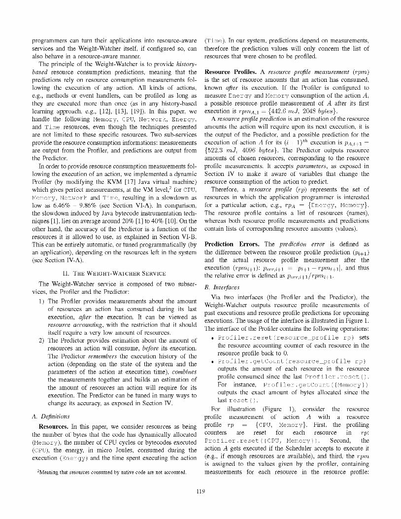
Via two interfaces (the Profiler and the Predictor), theWeight-Watcher outputs resource profile measurements ofpast executions and resource profile predictions for upcomingexecutions. The usage of the interface is illustrated in Figure 1.The interface of the Profiler contains the following operations:

* Profiler.reset(resource_profile rp) setsthe resource accounting counter of each resource in theresource profile back to 0.

* Profiler.getCount(resource_profile rp)outputs the amount of each resource in the resourceprofile consumed since the last Profiler .reset ().For instance, Profiler.getCount ( {Memory})outputs the exact amount of bytes allocated since thelast reset ().

For illustration (Figure 1), consider the resourceprofile measurement of action A with a resourceprofile rp {CPU, Memory}. First, the profilingcounters are reset for each resource in rp:Profiler.reset({CPU, Memory}). Second, theaction A gets executed if the Scheduler accepts to execute it(e.g., if enough resources are available), and third, the rpmis assigned to the values given by the profiler, containingmeasurements for each resource in the resource profile:

119

S El GDS ct: El

Fig. 1. Use of the interfaces of the Profiler and Predictor

rpm=Profiler.getCount({CPU, Memory}). Therpm, if used as exposed when encapsulating the execution ofan action, is then taken as input for the Predictor.The interface of the Predictor contains the following oper-

ations:

* Predictor.query(actionID aid) outputs a pre-

diction for a given action,* Predictor.update(actionID aid,resource-profile measurement rpm) updatesthe prediction of a given action with the output of theProfiler (rpm).

For a given action, the Predictor gets first setup with differentcombining strategies (i.e., the way the Predictor takes intoaccount past measurements to provide predictions, see Sec-tion IV-B) and parameters values (i.e., the state in which thesystem is before executing the action, see Section IV). Themethod Predi ctor.query() is the main entry point ofthe Predictor. It is used to know the amount of resources an

action A will require for its execution, before its execution.With this prediction, a decision making process can be run

to decide if this particular action should be executed or

not (Scheduler.canExecute(p)). If yes, the Profilerresets, then the action gets executed, and a rpm is outputfrom the Profiler. Now that a new measure is available, thepredictions for an upcoming execution can be refined viaPredictor.update () as shown in Figure 1.The Scheduler can thus base scheduling decisions by com-

paring the prediction and the actual amount of resources

available on the device. If the resource demand is greater thanwhat is currently left in the system or if the resources leftare detected to be shrinking (e.g., using threshold values) theScheduler can (1) postpone execution (until required resources

are available), (2) trigger resource shortage notification (so thatresource related errors can be avoided), or (3) pick an alter-native implementation (e.g., downgrade the level of service).The alternative implementations might be downloaded fromthe network, already loaded in main memory (i.e., ready toexecute) or on stable storage (i.e., ready to be loaded). Thisissue is out of scope of the paper and is not further discussed.

III. HISTORY-BASED PREDICTION

The role of the Predictor is to estimate, before the executionof the action, its upcoming resource consumption. In [2], theestimation of the memory consumption of a method is given bya parametric function, where the parameters of the function are

the actual method parameters. Let us formalize this functionas fmemory({,-i... x}, nM), where the xi are all the pa-rameters of the method m and f provides an estimation of theMemory allocated for an execution of m. In [2], the fMemoryfunction is created out of offline code analysis, whereas we

numerically approximate the same function, at runtime, forevery resource in the rp, i.e., not only Memory, by basingour prediction on actual measurements (the resource profilemeasurements, or rpms) output by the Profiler. Thus theestimation function f that we approximate is a generalizationof fMemory such that fVrcrp({xl, ... X4} in).To achieve the history-based prediction, the action first gets

executed and profiled. The Predictor remembers this rpm1, bystoring it in memory. When the piece of code is about to bereexecuted the prediction is in fact the first stored measurementgiven by the profiler (rpm,). After the second execution a new

rpm2 is generated by the Profiler. Both measurements (rpm,and rpm2) can thus be combined to refine the prediction (seeSection IV-B).An action that has a constant behavior in terms of

resource consumption is for example a method thatcomputes a Celsius temperature out of Fahrenheit(float fToCelsius(float fVal)). In this case

the estimation function and therefore the predictedvalue, is constant for each resource r for any execution:fr({fVal},fToCelsius) rpmfToCelsius,iPfToCelsius,i+1{r} = cr More generally, for constantactions (m is a constant action), the following holds:VxiVi, fr({xi,... Xn ,m) = rpmm,i+l = Pm,i+l{r} = cr.In theory, for such a simple behavior the memory cost forrecording the profiled value is equivalent to one int per

resource (resp. float according to the resource unit).In contrast, the execution of some other action can be

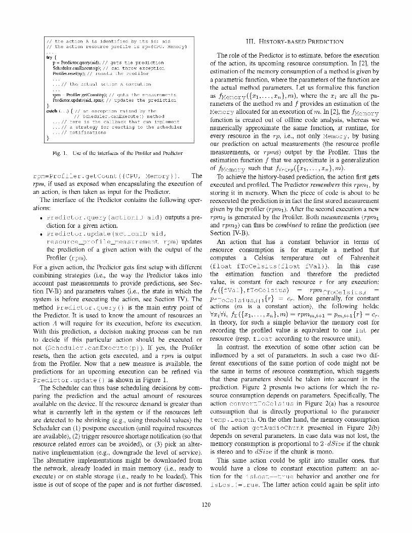
influenced by a set of parameters. In such a case two dif-ferent executions of the same portion of code might not bethe same in terms of resource consumption, which suggeststhat these parameters should be taken into account in theprediction. Figure 2 presents two actions for which the re-

source consumption depends on parameters. Specifically, Theaction convertToCelsius in Figure 2(a) has a resource

consumption that is directly proportional to the parametertemp. length. On the other hand, the memory consumptionof the action getAudioChunk presented in Figure 2(b)depends on several parameters. In case data was not lost, thememory consumption is proportional to 2 dSize if the chunkis stereo and to dSize if the chunk is mono.

This same action could be split into smaller ones, thatwould have a close to constant execution pattern: an ac-

tion for the isLost==true behavior and another one forisLost! =true. The latter action could again be split into

120

try {p = Predictor.query(aid); gets the predictionScheduler.canExecute(p); can throw exceptionProfiler.reset(rp); // resets the Profiler

../the actual action A execution

rpm= Profiler.getCount(rp); // gets the measurementsPredictor.update(aid, rpm); // updates the prediction

}catch(...){ an exception raised by the

//Scheduler.canExecute() method../here is the callback that can implement

a strategy for reacting to the scheduler...//}notifications

-ion A is ide L~d by its id: aid

void convertToCelsius(int[] temp) {for (int i=O; i<temp.length; i++) {

temp[i]=fToCelsius(temp[i]);

//The CPU consumption of the action dependson the array size (temp.length)

}(a) Single parameter: nbTemp

void getAudioChunk(Data d) {Header h d.getHeader(;boolean s h.isStereo(;int id = h.getld(;boolean isLost = (id != (currentld +1));if (isLost) {

//Detection of lost data ->Dedicated handling

else {int dSize = h.getDataLength(;if (s) {

int [][] buf = new int[dSize][2];processing of bi-channel audio signal

else {int [] buf = new int[dSize];

processing of mono channel audio signal

}}

(b) Several parameters: isLost, id and s

Fig. 2. Actions from which the execution patterns depend on input variablesand which thus have non-empty sets of parameters.

two actions, one for the treatment of the stereo-channel signaland another one for treatment of the mono-channel signal, andso on. Of course it is cumbersome for a developer to unfoldloops manually or even split an action into smaller ones, whichis the main reason why the Predictor needs to take parameters(e.g., isLost, id, s) into account for storing and buildingpredictions.

IV. LIGHTWEIGHT WEIGHT-WATCHER IMPLEMENTATION

For obvious memory reasons, the Predictor does not keeptrack of every past parameter value and corresponding resourceconsumptions. Thus, it must sample continuous parameters toremember past executions, i.e., parameter values that comeclose are considered equal and will get the same prediction.Taking the example from Figure 2 (a) two executions ofcunvertToCelsius ( ) with arrays of different sizes (theparameter of the action being temp. length) might returnthe exact same prediction. How close two parameter values areis defined by: (1) the parameter bounds, and (2) the samplingprecisions.

The simplest data structure and the one that has the small-est overhead for storing samples of one single continuousparameter is an array. The size of this array depends onthree factors: the minimum value of the parameter (min), itsmaximum value (max), the number of intervals (k) betweenthe min and the max and the number of resources (r)in the resource profile taken into consideration. If measuresare stored as integers, for a continuous parameter having amMi = 0, max = 500, and k = 50, the width of each interval(A = (max -min)/k) is 10 and the size of the array is then

50 sizeuf (int) r. A is further refered to as the precisionof a certain parameter. This means that every action executingwith parameter values in range [10..19] are considered thesame, in other words, the prediction for an upcoming executionin this particular interval will be the same.

For one parameter, the size of the array is defined by k r t,and is generalized as H|p1Par k, r t for multiple parameters,where r is the number of resources, NbPar the number ofparameters, kp their corresponding intervals and t the size ofthe type of data stored.An analysis of this function trivially shows that the memory

used for storage is mostly influenced by the number of pa-rameters (nbPar) and the desired precision for the predictionof values of each parameter (kp). Both t and the number ofresources r are relatively small, meaning that it is not bymodifying t and r that the array memory consumption willbe influenced. Thus, if the service must dynamically adapt itsresource consumption (the memory consumption of the arrayin that case), it must be able to tune the kp service parametersto still be able to take a constant nbPar number of parametersinto account.

A. Adaptive Array

A programmer might not always be able to know a priorithe exact range of values that a parameter might take duringall executions of a certain action. Cases can happen when aparameter takes a value which is outside its initial range. Ifin a particular execution the parameter value v falls outsideof its [min.max] range, two possibilities arise for storing thevalue:

1) Extending the size of the array and keeping the precision(A) constant.

2) Keeping the same array size and decreasing the precisionA.

Keeping the precision (A) constant. In the first case, therange of a parameter is increased while A stays constant,resulting in an increase in the array size (ki /). Consideringthe example from last section where a parameter is initializedwith the values min = 0, max = 500 and k 50 (A = 10).The action is now executed with v = 512 [0..500]. Therange is therefore forced to grow to [0..520] to include the newv (two intervals of size A = 10 are added) and the number ofintervals reaches k = 12. This strategy results in an increaseof the memory taken by the resource profile (directly related tok as exposed in Section IV) especially when the out of rangevalue is very far from the min (resp. max). The number ofadditional intervals kadd is defined as (v- max) / A] (resp.F(min -v) / A]).Keeping the array size constant. In order to keep the size

of the array constant, the range of a parameter is modified bydecreasing the array precision (A \). Looking at the previousexample, when the action is executed with v = 512, severalsolutions can be followed:

Keeping the A of every cell but the last one constant,A0_.48 = 10 and increase the A of the last cell to take

121

the parameter value into account, A49 = 22. The lastcell of the array of the concerned parameter has a worseprecision than the other cells (because it is larger) andthe total range of values is changed to [0..512], allowingthe new value to be stored in the array.Increase the A of every cell: Vi, Ai = 11, in which casethe total range is changed to [0..550]. In order to do this,the values for each new cell need to be recomputed. Asa cell in the new array will be a linear combination ofcells spanning the same range in the old array, dedicatedcalculation for computing the values must be executed torepopulate the array.

These reactions to a parameter value that is out of rangeof the prediction array can be issued by (1) the system insituations where the need of either precision on measurementsor available resources is predominent (automatic adaptivity) or(2) by the programmer in order to have control over the contentof the resource profile.

B. Combining Strategies

A combining strategy is represented by the function Pi+,g(pi..i, rpmT..i) meaning the prediction for the upcoming(i + i)th execution can be computed with the prediction ofthe last executions P1..i = p...l. , pi and/or the resourceprofile measurements rpml..i {rpmi,...,rpmij of thepast executions. To have an optimal prediction, the strategiesshould minimize the prediction error under the constraintthat the combining strategies must be as frugal as possible,i.e., being the least consuming in terms of CPU and Memoryusage.

Overwriting Strategy (OS). The first and simplest strategyto update its prediction Pi+, is to state that the (i + i)thexecution will have the exact same resource need as the jthoutput from the Profiler. In other words, the resource profilermeasurement rpmi is used as is in order to predict the nextexecution, see (1) in Figure 3.

(1) Overwriting Strategy (OS): {Pi+1=rpmi (i > 1)

(2) Adapting Strategy (AS): {P i+2rpr (i > 2)

{P2 =rPMi(3) Low-Pass Filter (LPF): 8Xpi+2XrpTn (i > 2)

P2p=rPM I(4) Global Average (GA): rp Pi (i-)+rP (i > 2)

Fig. 3. Combining strategies

Overwriting the prediction with the rpm at every executionstates that an action stabilizes completely over time, or that theaction does not depend on any parameter. It is the mostfrugal,in the sense that no memory on the history of measurementsis kept and that the actual computation is simply a valuereplacement in the prediction array.

Adapting Strategy (AS). The second strategy is to do anaverage of the last (ith) prediction pi with the correspondingmeasure rpmi. The strategy is defined by (2) in Figure 3.The last rpm influences the prediction twice as less as in the

overwriting strategy, adding an addition and a division to thecomplexity.Low-Pass Filter (LPF). The low-pass filter gives predefined

weight to both the prediction (80%) and the actual measure-ment (20%) as (3) in Figure 3. It adds two multiplicationsto the complexity of the adapting strategy. Note that for everystrategy until now, a variable containing the measurement fromthe profiler rpmi and the prediction itself pi was enough tocompute the new prediction Pi+± (pi and Pi+± correspond tothe same slot in the array).

Global Average (GA). A global average is also proposedas (4) in Figure 3. Note that every past resource profiles do notneed to be stored, as the last prediction pi and i are enough toreconstruct the sum from 1 to i- 1. This basically means thatnot only the last prediction must be kept but also i, the numberof measurements the profiler has output for that particularprediction. In fact, an array for storing the prediction and anadditional array (of same size) must be used for storing thecorresponding number of iterations, i.e., doubling the memoryusage of the combining strategy. In number of mathematicaloperations, it has one multiplication less, and adds only onesubtraction (i -1) to the low-pass filter, but in practice, thestrategy is more expensive as more accesses in memory mustbe made (for getting i) instead of using constants as in thelow-pass filter.The prediction errors of each combining strategy are sum-

marized in Figure 4 and will be exposed as a performancemetric in Section VI.

(1) Os: Perr,i+i = lrpm,- rpm+l, (i > 1)(2) AS: p,,,i+I = 1 rpm 1X ) -rpmi+ (i > 2)(3) LPF:pe,,i+l =1 1r rpm(, 1 -rpmi+1 (i > 2)(4) GA: p 1 rpmi 1 (i > 2)

Fig. 4. Prediction errors

C. First execution issue or sharing resource profile as initialdata

It is only after the first execution of the action that anrpm is output and thus a prediction can be created3. Weconsider the following solutions to this problem of havinginitial predictions:

* Share resource profile: even though resource units arenot completely portable (e.g., heterogenous VM, CPUs,devices can lead to different rpm for the same action),they can be used as an initial resource profile measure-ment rpmo for the first prediction P1 = rpmo and thenrefined by the different combining strategies.

* Use existing solutions, as exposed in [12] by first ex-ecuting a training phase, that consists in executing theaction various times to get first measurements, thenoptionally run an offline learning phase and finally usethe predictions at runtime.

3To be exact, for a predefined parameter range R, there exists only an rpmthus a prediction after an execution of the action in the same condition, i.e.,with a parameter value v C R.

122

V. IMPLEMENTATION

The Weight-Watcher service is composed of (1) modifica-tions to the KVM in order to implement the Profiler and (2)Java classes implementing the Predictor.

A. ProfilerWe propose generic modifications to a VM that implement

the Profiler. The dynamic Profiler accounts for Memory (inbytes), CPU (in number of bytecodes), Tlime (in ,us) andNetwork (in bytes/s) while the program is actually running.For doing so, counters are added to the VM threads, that areincremented while the bytecodes are executed by the virtualmachine. The CPU counter must be incremented as manytimes as bytecodes are executed in the current thread (easilyachieved in an interpreted VM as KVM [17]), whereas theMemory counter is incremented by the size of the data thatis allocated by the current thread (modifications to the VMmemory management of KVM).

For CPU, a counter (an array of 256 ints) keeps trackof which bytecodes are executed and how many times, sothat it is summed up when Profiler.getCount ( {CPU})is called, providing the actual number of bytecodes executedsince the last Profiler.resetCount(). It is also pos-sible to output the CPU counter array (which bytecode wasexecuted how many times, and not only the total number ofbytecodes executed) to get a more fine-grained measurementof the execution and could be used as a time analysis factorif a per-bytecode time consumption model is available.Energy (in ,uJ) is deduced from a per-bytecode energy con-

sumption model [11], i.e., a table containing for each bytecodea corresponding energy cost (aggregating CPU instructions andmemory energy costs). An array of 256 floats contains theper-bytecode energy consumption which is multiplied with theinternal CPU counter array to get an estimation of the actionEnergy consumption.

Tlime is the time spent in the given piece of code ex-cluding the time executing higher priority tasks that couldhave preempted the current action. The implementation of theTlime counter incrementation is slightly more difficult thanCPU accounting as threads can be preempted in the VM.The Network resource is not profiled in the VM itself,

but at the library level; it basically adds up the number ofbytes sent out by the action, in concordance with the Timeconsumption. This resource will e.g. help to detect networkcongestion, as exposed in the introductory example, when usedwith blocking protocols as HTTP or TCP.

In KVM, memory usage for primitive types is given as 1byte for a byte, 2 bytes for a char, 4 bytes for an mntor a float and 8 bytes for a double or a long. Theseprimitive types can be encapsulated in Ob j e ct s or containedin arrays. An Object in KVM has an overhead of 12 bytesand an array (arrayStruct) 16 bytes.Memory usage of simple data structures can therefore be

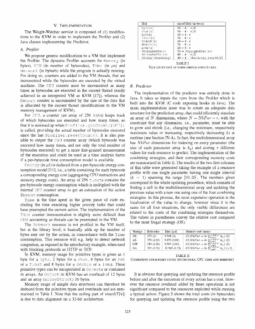
deduced from the primitive types and overheads and are sum-marized in Table I. Note that the ceiling part of sizeof(T[x])is due to data alignment on a 32-bit architecture.

T[x] [ sizeof(T[x]) (in bytes)byte [x] 16 + 4 [x14]char [x] 16 + 4 [x12]int [x] 16 + 4 xfloat [x] 16 + 4 xObject [x] 16 + 4 xdouble[x] 16 + 8 xlong[x] 16 + 8 xStringBuffer() 72 = StringBuffer(16)StringBuffer(x) 40 + 4 *[x2]String(charArray) 40 + 4 2]charArray.length/2

TABLE ISIZE (IN BYTES) OF SOME SIMPLE STRUCTURES

B. Predictor

The implementation of the predictor was entirely done inJava. It takes as inputs the rpm from the Profiler which isbuilt into the KVM (C code exposing hooks in Java). Themain implementation issue was to create an adequate datastructure for the prediction array, that could efficiently simulatean array of N dimensions, where N = NbPar + r, with theconstraint that any dimension, i.e., parameter, must be ableto grow and shrink (i.e., changing the minimum, respectivelymaximum value or increasing, respectively decreasing k) atruntime (see Section IV-A). In fact, the multidimensional arrayhas NbPar dimensions for indexing on every parameter (thesize of each parameter array is kp) and storing r differentvalues for each resource to predict. The implementation of thecombining strategies, and their corresponding memory costsare summarized in Table II. The results of the two first columnsof this table were generated taking the example of a resourceprofile with one single parameter having one single interval(k = 1) spanning the range [10..20]. The numbers givencorrespond to the whole updating procedure, which consists offinding a cell in the multidimensional array and updating theprevious value with a new one using one of the four combiningstrategies. In this process, the most expensive operation is thelocalization of the value to change, however since it is thesame for all four situations, the only visible differences arerelated to the costs of the combining strategies themselves.The values in parentheses convey the relative cost comparedto the most frugal strategy (OS).

Strategy Bytecodes Time [,us] Memory cost (array)OS 273 (1) 9.348 (1) O(NbPar + 4rflH_'6 kp) (1)AS 279 (1.02) 9.473 (1.01) O(NbPar + 4r flb"_P kkc) (1)LPF 283 (1.03) 9.597 (1.02) O(NbPar + 4r H nt_Par kp) (1)GA 332 (1.21) 11.565 (1.23) O(NbPar + 8rHr nl Pa kCp ) (>2)

TABLE IICOMBINING STRATEGIES COSTS (BYTECODES, CPU TIME AND MEMORY)

It is obvious that querying and updating the resource profilebefore and after the execution of every action has a cost. How-ever the resource overhead added by these operations is notsignificant compared to the resources exploited while runninga typical action. Figure 5 shows the total costs (in bytecodes)for querying and updating the resource profile using the two

123

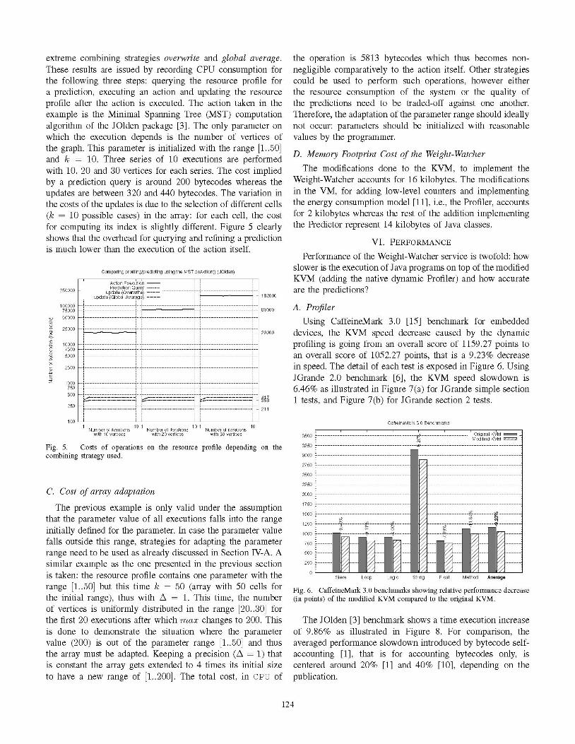
extreme combining strategies overwrite and global average.These results are issued by recording CPU consumption forthe following three steps: querying the resource profile fora prediction, executing an action and updating the resourceprofile after the action is executed. The action taken in theexample is the Minimal Spanning Tree (MST) computationalgorithm of the JOlden package [3]. The only parameter onwhich the execution depends is the number of vertices ofthe graph. This parameter is initialized with the range [1..50]and k = 10. Three series of 10 executions are performedwith 10, 20 and 30 vertices for each series. The cost impliedby a prediction query is around 200 bytecodes whereas theupdates are between 320 and 440 bytecodes. The variation inthe costs of the updates is due to the selection of different cells(k = 10 possible cases) in the array: for each cell, the costfor computing its index is slightly different. Figure 5 clearlyshows that the overhead for querying and refining a predictionis much lower than the execution of the action itself.

250000

1000007500050000

25000

1000075005000

Comparing profiling/predicting using the MST.doAction( (JOlden)

Action ExecutionPrediction Query

update (Overwrite).update (Global Average) ----

2500 _

co

co

-ocJ)>1-0

z 1000750500

250

100

Number of iterations Number of iterations Number of iterationswith 10 vertices with 20 vertices with 30 vertices

Fig. 5. Costs of operations on the resource profile depending on thecombining strategy used.

C. Cost of array adaptation

The previous example is only valid under the assumptionthat the parameter value of all executions falls into the rangeinitially defined for the parameter. In case the parameter valuefalls outside this range, strategies for adapting the parameterrange need to be used as already discussed in Section IV-A. Asimilar example as the one presented in the previous sectionis taken: the resource profile contains one parameter with therange [1..50] but this time k = 50 (array with 50 cells forthe initial range), thus with A = 1. This time, the numberof vertices is uniformly distributed in the range [20..30] forthe first 20 executions after which max changes to 200. Thisis done to demonstrate the situation where the parametervalue (200) is out of the parameter range [1.50] and thusthe array must be adapted. Keeping a precision (A = 1) thatis constant the array gets extended to 4 times its initial sizeto have a new range of [1.200]. The total cost, in CPU of

182000

the operation is 5813 bytecodes which thus becomes non-negligible comparatively to the action itself. Other strategiescould be used to perform such operations, however eitherthe resource consumption of the system or the quality ofthe predictions need to be traded-off against one another.Therefore, the adaptation of the parameter range should ideallynot occur: parameters should be initialized with reasonablevalues by the programmer.

D. Memory Footprint Cost of the Weight-Watcher

The modifications done to the KVM, to implement theWeight-Watcher accounts for 16 kilobytes. The modificationsin the VM, for adding low-level counters and implementingthe energy consumption model [11], i.e., the Profiler, accountsfor 2 kilobytes whereas the rest of the addition implementingthe Predictor represent 14 kilobytes of Java classes.

VI. PERFORMANCE

Performance of the Weight-Watcher service is twofold: howslower is the execution of Java programs on top of the modifiedKVM (adding the native dynamic Profiler) and how accurateare the predictions?

80000 A. ProfilerUsing CaffeineMark 3.0 [15] benchmark for embedded

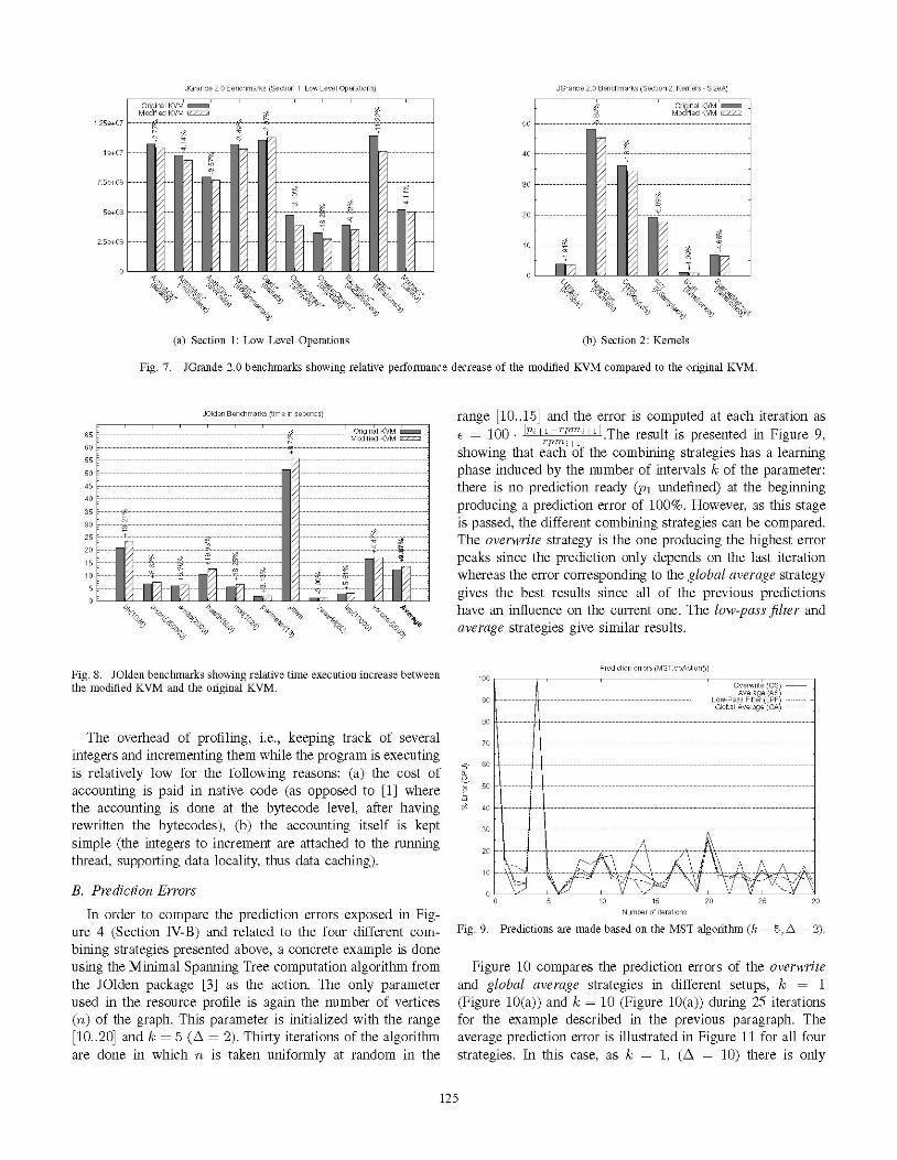
20000 devices, the KVM speed decrease caused by the dynamicprofiling is going from an overall score of 1159.27 points toan overall score of 1052.27 points, that is a 9.23% decreasein speed. The detail of each test is exposed in Figure 6. UsingJGrande 2.0 benchmark [6], the KVM speed slowdown is6.46% as illustrated in Figure 7(a) for JGrande simple section1 tests, and Figure 7(b) for JGrande section 2 tests.

211

CaffeineMark 3.0 Benchmarks

3500

3250

3000

2750

2500

2250

2000

1750

1500

1250

1000

750

500

250

0Sieve Loop Logic String Float Method Average

Fig. 6. CaffeineMark 3.0 benchmarks showing relative performance decrease(in points) of the modified KVM compared to the original KVM.

The JOlden [3] benchmark shows a time execution increaseof 9.86% as illustrated in Figure 8. For comparison, theaveraged performance slowdown introduced by bytecode self-accounting [1], that is for accounting bytecodes only, iscentered around 20% [1] and 40% [10], depending on thepublication.

124

JGrande 2.0 Benchmarks (Section 1: Low Level Operations)

1 .25e+07

1 e+07

7.5e+06

5e+06

2.5e+06

C, 1% 0 0.44."- 1, A .&--4W- lpip 6411".

1.1 1.1 6/- \ ,190-1.1

(a) Section 1: Low Level Operations (b) Section 2: Kernels

Fig. 7. JGrande 2.0 benchmarks showing relative performance decrease of the modified KVM compared to the original KVM.

JOlden Benchmarks (time in seconds)

65

60

55

50

45

40

35

30

25

20

15

10

5

0

Fig. 8. JOlden benchmarks showing relative time execution increase betweenthe modified KVM and the original KVM.

The overhead of profiling, i.e., keeping track of severalintegers and incrementing them while the program is executingis relatively low for the following reasons: (a) the cost ofaccounting is paid in native code (as opposed to [1] wherethe accounting is done at the bytecode level, after havingrewritten the bytecodes), (b) the accounting itself is keptsimple (the integers to increment are attached to the runningthread, supporting data locality, thus data caching).

B. Prediction Errors

In order to compare the prediction errors exposed in Fig-ure 4 (Section IV-B) and related to the four different com-bining strategies presented above, a concrete example is doneusing the Minimal Spanning Tree computation algorithm fromthe JOlden package [3] as the action. The only parameterused in the resource profile is again the number of vertices(n) of the graph. This parameter is initialized with the range[10..20] and k = 5 (A = 2). Thirty iterations of the algorithmare done in which n is taken uniformly at random in the

range [10..15] and the error is computed at each iteration ase 100 - I1+`pmmi+1.The result is presented in Figure 9,showing that each of the combining strategies has a learningphase induced by the number of intervals k of the parameter:there is no prediction ready (P1 undefined) at the beginningproducing a prediction error of 100%. However, as this stageis passed, the different combining strategies can be compared.The overwrite strategy is the one producing the highest errorpeaks since the prediction only depends on the last iterationwhereas the error corresponding to the global average strategygives the best results since all of the previous predictionshave an influence on the current one. The low-pass filter andaverage strategies give similar results.

Prediction errors (MST.doActiono)

c-IL

100

90

80

70

60

50

40

30

20

10

0 5 10 15 20 25Number of iterations

Fig. 9. Predictions are made based on the MST algorithm (k = 5, Ai

30

2).

Figure 10 compares the prediction errors of the overwriteand global average strategies in different setups, k = 1(Figure 10(a)) and k = 10 (Figure 10(a)) during 25 iterationsfor the example described in the previous paragraph. Theaverage prediction error is illustrated in Figure 11 for all fourstrategies. In this case, as k = 1, (A = 10) there is only

125

JGrande 2.0 Benchmarks (Section 2: Kernels SizeA)

100

90

80

70

5~IL

6,

6U

50

40

30

20

10 15 20 25 0 5 10 15

(a) k= 1,lA 10 (b) k = 10, I1

Fig. 10. Different prediction errors depending on k (thus A) for overwrite and global average strategies.

Average Prediction errors (MST.doActiono)

k=1, A= 10 k=10, A= 1

Fig. 11. Average prediction errors (10'000 iterations) depending on k (thusA) for different combining strategies.

one integer to store in the prediction array, i.e., a memory

cost of 4 bytes. It is also the only value which can be usedin next iterations to predict the resource consumption of thesystem. With this very simple prediction setup, the overwritecombining strategy gives errors going up to 70%. In fact, thevery worst case, for this strategy is when an execution withn = 10 is directly followed by an execution with n = 15.The graphs show that the complexity of the combining tasksis proportional to their accuracy, as summarized in Figure 11.

Figure 10(b) shows the prediction errors of the same action,with k = 10 intervals of size A 1 ([min..max] = [10.20]).A prediction array of size 10 must be kept in memory, whichrepresents 40 bytes. The graph clearly shows that sampling theparameter increases the precision of the prediction drastically.In fact, the only drawback (apart from the increased memory

consumption) is that 5 executions were needed to initializethe array (recalling that n is chosen uniformly at random inthe range [10..15]) for which the error equals 100%, whichexplains the 5 peaks at the beginning of the graph. An

interesting aspect to notice is that one can naturally think thatthe error should be 0 after the five first steps used for settingthe values in the array. However the MST algorithm is nottotally deterministic since it uses random numbers to computedistances between edges. Therefore even if two executions are

done with the same parameter, their CPU consumption will beclose, but not precisely the same, leading to the errors observedeven when A = 1.The prediction errors are averaged, for each combining

strategy, with 10'000 iterations (Figure 11). The histogramshows (1) that the overall accuracy of combining strategiesare proportional to their complexity, and (2), that with a very

small A, all combining strategies behave comparably.Global average, in general, is superior in terms of accuracy,

which seems somehow negligible when its complexity, bothin terms of memory and CPU consumption (see Table II), iscompared to the second best combining strategy: Low-PassFilter.

VII. RELATED WORK

Predicting resource consumption of code is hard (in some

cases undecidable [2]), and typically requires a lot of re-

sources for its own purpose, thus making it a real challengeon resource-constrained devices. Moreover, the estimationspredicted for a piece of code are typically not portable fromone device to another and thus can typically not be computedin advance and shared amongst devices: internal object layoutand header size are implementation specific, and, above all,battery and CPU consumption of a piece of code are devicespecific. It is shown, for instance in [4] that there is a strongcorrelation between the number of bytecodes executed andthe elapsed CPU time, but this correlation is application-specific and obviously depends on the given VM/OS/hardwarecombination. However, in [9], an attempt is made to definea set of portable resource metrics which are converted toplatform-specific values thanks to statically computed conver-

sion factors.

126

90

80

70

cEIL

6U

50

40

30

20

10

20 25

100I

,

.cJp

Static analysis of memory [2], [5], [8], [18] and time [7],[14] can provide upper bounds of memory, respectively timeusage of a given piece of code, providing strong guaranteesthat the code will never exceed the estimation. Determiningmemory upper bounds may improve memory management,e.g., for stack-based allocation of dynamic objects, or forcreating parametric memory-allocation certificates [2]. Worst-case execution times are key in computing scheduling schemesthat satisfy all timing constraints [7]. However, static load-time code analysis is itself very demanding in terms ofresources, and is therefore not an ideal candidate for resource-constrained devices, as it may cause significant latencies (i.e.,service downtime). In [2] most of the static analysis includ-ing the execution of the core components (finding creationsites, computing control-state invariants, inductive variablesand Ehrhart polynomials) took close to 30 seconds on anIntel Pentium IV 3GHz CPU. In contrast, the approach weconsider here consists in loading and executing the code onthe fly and performing the analysis at runtime (during the firstexecutions), giving resource consumption approximations aftera few executions.

In [1], [2], the amount of memory that is allocated by nativecode or by the virtual machine itself cannot be measured,respectively estimated. Section V-A shows that applying modi-fications at the VM level allows to quantify the memory that isallocated by the VM itself, e.g., the overhead of data structures.The work in [13] is close to ours since the goal also is

to make programs change behavior depending on resourcepredictions. Nevertheless, their predictions are based on (1)desktop linux kernel outputs and (2) history of executions. Thefirst is not targetting embedded devices and the second relieson log files (stable storage) and statistical machine learning,which are both way too resource demanding for the embeddeddevices we target.

VIII. CONCLUDING REMARKS

This paper introduces the Weight-Watcher service. Thisservice aims at providing resource consumption measurementsand estimations for software executing on resource-constraineddevices. As a consequence, the service enables software com-ponents to continuously adapt and optimize their quality ofservice according to resource availability. We presented animplementation of the service that includes a Profiler (inthe KVM) as well a library of Java classes encapsulatingresource prediction. The evaluation shows that there is stillroom for improvement on the implementation of the Profiler.In particular, it could be interesting to include preparationsequences in order to reduce the cost of profiling in interpretedvirtual machines. It would also be interesting to preciselycapture the trade-off between the memory consumption of the

Predictor and the accuracy of the predictions.

REFERENCES

[1] W. Binder and J. Hulaas. A portable cpu-management framework forjava. IEEE Internet Computing, 8(5):74-83, 2004.

[2] V. Braberman, D. Garbervetsky, and S. Yovine. A static analysis forsynthesizing parametric specifications of dynamic memory consumption.Journal of Object Technology, 5(5):31-58, June 2006.

[3] B. Cahoon and K. S. McKinley. Data flow analysis for softwareprefetching linked data structures in java. In PACT '01: Proceedings ofthe International Conference on Parallel Architectures and CompilationTechniques, pages 280-291, Barcelona, September 2001.

[4] A. Camesi, J. Hulaas, and W. Binder. Continuous Bytecode InstructionCounting for CPU Consumption Estimation. In QEST '06: (3rdInternational Conference on the Quantitative Evaluation of SysTems).IEEE Computer Society Press, 2006.

[5] W.-N. Chin, H. H. Nguyen, S. Qin, and M. C. Rinard. Memory usageverification for oo programs. In SAS '05: Proceedings of the 12th StaticAnalysis Symposium, pages 70-86, 2005.

[6] C. Daly, J. Horgan, J. Power, and J. Waldron. Platform independentdynamic java virtual machine analysis: the java grande forum bench-marking suite. In Proceedings of the joint ACM-ISCOPE conference onJava Grande, pages 106-115, Palo Alto, 2001.

[7] C. Ferdinand. Worst case execution time prediction by static programanalysis. IPDPS '03: Proceedings of the 17th International Parallel &Distributed Processing Symposium, 03:125a, 2004.

[8] M. Hofmann and S. Jost. Static prediction of heap space usage for first-order functional programs. In POPL '03: Proceedings of the 30th ACMSIGPLAN-SIGACTsymposium on Principles ofprogramming languages,pages 185-197, New York, NY, USA, 2003. ACM Press.

[9] E.-N. Huh, L. Welch, B. Shirazi, and C. Cavanaugh. Heterogeneousresource management for dynamic real-time systems. In HCW 2000:9th Heterogeneous Computing Workshop, page 287, 2000.

[10] J. Hulaas and W. Binder. Program transformations for portable cpuaccounting and control in java. In PEPM '04: Proceedings of the 2004ACM SIGPLAN symposium on Partial evaluation and semantics-basedprogram manipulation, pages 169-177, New York, NY, USA, 2004.ACM Press.

[11] S. Lafond and J. Lilius. An energy consumption model for an embeddedjava virtual machine. In ARCS '06: Proceedings of the 19th InternationalConference on Architecture of Computing Systems, pages 311-325,Frankfurt, March 2006.

[12] D. Narayanan, J. Flinn, and M. Satyanarayanan. Using history toimprove mobile application adaptation. In WMCSA '00: Proceedings ofthe 3rd IEEE Workshop on Mobile Computing Systems and Applications,pages 31-. IEEE Computer Society, 2000.

[13] D. Narayanan and M. Satyanarayanan. Predictive resource managementfor wearable computing. In MobiSys '03: Proceedings of the 1stinternational conference on Mobile systems, applications and services,pages 113-128, New York, NY, USA, 2003. ACM Press.

[14] C. Y Park. Predicting program execution times by analyzing static anddynamic program paths. Real-Time Syst., 5(1):31-62, 1993.

[15] Pendragon Software Corporation. CaffeineMark 3.0 for EmbeddedDevices. http://www.benchmarkhq.ru/cm30/info.html.

[16] M. Satyanarayanan and D. Narayanan. Multi-fidelity algorithms forinteractive mobile applications. Wireless Networks, 7(6):601-607, 2001.

[17] Sun Microsystems. J2ME Building Blocks for Mobile Devices, WhitePaper on KVM and the Connected, Limited Device Configuration(CLDC), May 2000. http://java.sun.com/products/cldc/wp/KVMwp.pdf.

[18] L. Unnikrishnan, S. D. Stoller, and Y. A. Liu. Optimized live heapbound analysis. In VMCAI '03: Proceedings of the 4th InternationalConference on Verification, Model Checking, and Abstract Interpreta-tion, pages 70-85, London, UK, 2003. Springer-Verlag.

[19] R. Wolski, N. T. Spring, and J. Hayes. The network weather service: adistributed resource performance forecasting service for metacomputing.Future Generation Computer Systems, 15(5-6):757-768, 1999.

127