the welfare effects of vertical integration in
TRANSCRIPT

http://www.econometricsociety.org/
Econometrica, Vol. 86, No. 3 (May, 2018), 891–954
THE WELFARE EFFECTS OF VERTICAL INTEGRATIONIN MULTICHANNEL TELEVISION MARKETS
GREGORY S. CRAWFORDDepartment of Economics, University of Zurich
ROBIN S. LEEDepartment of Economics, Harvard University
MICHAEL D. WHINSTONDepartment of Economics and Sloan School of Management, MIT
ALI YURUKOGLUGraduate School of Business, Stanford University
The copyright to this Article is held by the Econometric Society. It may be downloaded, printed and re-produced only for educational or research purposes, including use in course packs. No downloading orcopying may be done for any commercial purpose without the explicit permission of the Econometric So-ciety. For such commercial purposes contact the Office of the Econometric Society (contact informationmay be found at the website http://www.econometricsociety.org or in the back cover of Econometrica).This statement must be included on all copies of this Article that are made available electronically or inany other format.

Econometrica, Vol. 86, No. 3 (May, 2018), 891–954
THE WELFARE EFFECTS OF VERTICAL INTEGRATIONIN MULTICHANNEL TELEVISION MARKETS
GREGORY S. CRAWFORDDepartment of Economics, University of Zurich
ROBIN S. LEEDepartment of Economics, Harvard University
MICHAEL D. WHINSTONDepartment of Economics and Sloan School of Management, MIT
ALI YURUKOGLUGraduate School of Business, Stanford University
We investigate the welfare effects of vertical integration of regional sports networks(RSNs) with programming distributors in U.S. multichannel television markets. Verti-cal integration can enhance efficiency by reducing double marginalization and increas-ing carriage of channels, but can also harm welfare due to foreclosure and incentivesto raise rivals’ costs. We estimate a structural model of viewership, subscription, dis-tributor pricing, and affiliate fee bargaining using a rich data set on the U.S. cable andsatellite television industry (2000–2010). We use these estimates to analyze the impactof simulated vertical mergers and divestitures of RSNs on competition and welfare, andexamine the efficacy of regulatory policies introduced by the U.S. Federal Communi-cations Commission to address competition concerns in this industry.
KEYWORDS: Vertical integration, foreclosure, double marginalization, raising rivals’costs, cable television.
1. INTRODUCTION
THE WELFARE EFFECTS OF VERTICAL INTEGRATION is an important but controversial is-sue. The theoretical literature on the pro- and anti-competitive impacts of vertical in-tegration is vast (cf. Perry (1990), Rey and Tirole (2007), Riordan (2008), Bresnahanand Levin (2013)), and typically contrasts potential efficiencies related to the elimina-tion of double marginalization (Spengler (1950)) and the alignment of investment incen-tives (Willamson (1985), Grossman and Hart (1986)) with the potential for losses arisingfrom incentives to foreclose rivals and raise their costs (Salop and Scheffman (1983),Krattenmaker and Salop (1986), Hart and Tirole (1990), Ordover, Saloner, and Salop(1990)). Despite a growing literature, empirical evidence on the quantitative magnitudesof these potential effects, and the overall net welfare impact, is still limited.
This paper quantifies the welfare effects of vertical integration in cable and satellitetelevision in the context of high-value regional sports programming in the United States.
Gregory S. Crawford: [email protected] S. Lee: [email protected] D. Whinston: [email protected] Yurukoglu: [email protected] would like to thank the editors, six anonymous referees, and numerous individuals and seminar par-
ticipants for helpful comments; and ESRC Grant RES-062-23-2586 (Crawford), the NYU Stern Center forGlobal Economy and Business (Lee), and the Toulouse Network for Information Technology and the NSF(Whinston) for support. All errors are our own.
© 2018 The Econometric Society https://doi.org/10.3982/ECTA14031

892 CRAWFORD, LEE, WHINSTON, AND YURUKOGLU
Whether the ownership of content by distributors harms welfare has been at the heart ofthe debate over recently approved (e.g., Comcast and NBC in 2011), abandoned (e.g.,Comcast and Time Warner in 2015), and proposed (e.g., AT&T and Time Warner in2016) mergers in the television industry. The attention that these mergers have attracted ispartly due to the industry’s overwhelming reach and size: over 80% of the approximately120 million television households in the U.S. subscribe to multichannel television, andthe mean individual consumes about four hours of television per day.1 Regional sportsprogramming is a large part of this industry, receiving $4.1 billion out of over $30 billionper year in negotiated affiliate fees paid by distributors to all content providers, and anadditional $700 million per year in advertising dollars.2
Our focus on the multichannel television industry, and in particular regional sportsprogramming, is driven by several factors that create empirical leverage to address thisquestion. First, there is significant variation across the industry in terms of ownershipof regional sports content by cable and satellite distributors, also referred to as multi-channel video programming distributors (MVPDs). Although this variation is primarilyat the national level for most channels, regional sports networks (RSNs) are present insmaller geographic areas, and there is useful variation in ownership patterns both acrossregions and over time. Additionally, the industry is the subject of significant regulatoryand antitrust attention in addition to merger review, including the application of “pro-gram access rules” and exceptions to this rule, such as the “terrestrial loophole” whichexempted certain distributors from supplying integrated content to rivals.
There are two key components of our analysis. The first is the construction of a com-prehensive data set on the U.S. multichannel television industry, collected and synthe-sized from numerous sources. The data set comprises aggregate and individual-level con-sumer viewership and subscription patterns, channel ownership and integration status,and prices, quantities, and channel carriage “lineups” for cable and satellite bundles atthe local market level for the years 2000 to 2010.
The second component is the specification and estimation of a structural model of themultichannel television industry that captures consumer viewership and subscription de-cisions, MVPD pricing and carriage decisions, and bargaining between MVPDs and con-tent providers. We significantly extend the model of Crawford and Yurukoglu (2012) byconstructing an empirical framework suitable for the analysis of vertical integration andmergers. Our model incorporates integrated firms’ incentives to foreclose rivals’ accessto inputs, the potential for double marginalization, and the possibility of imperfect co-ordination and internalization within an integrated firm. This last feature is one of thenovel aspects of our approach, as we estimate, rather than impose, the degree to whichfirms internalize the profits of integrated units when distributors make pricing and chan-nel carriage decisions, and channels decide to supply or foreclose rival distributors. Givenour goal to evaluate whether vertical integration improves or worsens welfare due to im-provements in internal efficiency or increases in foreclosure of rivals, taking this approachavoids building into our model the assumption that these two effects actually happen tothe extent predicted by theory. For example, only very simple views of the firm imply thatintegrated firms behave as if they are under unitary control, and managers of integratedfirms may well either not consider or over-react to the gains that can be reaped fromforeclosure.
1http://www.nielsen.com/us/en/insights/news/2016/nielsen-estimates-118-4-million-tv-homes-in-the-us--for-the-2016-17-season.html, http://www.nielsen.com/content/dam/corporate/us/en/reports-downloads/2016-reports/q3-2016-total-audience-report.pdf, accessed on March 13, 2016.
2SNL Kagan.

WELFARE EFFECTS OF VERTICAL INTEGRATION IN TELEVISION MARKETS 893
An important input into identifying these effects is our estimates of the change in dis-tributor profits from the addition or removal of an RSN from any of its programmingbundles. We use the relationship between distributors’ market shares and channel car-riage, as well as observed viewership patterns and negotiated affiliate fees, to infer thevalues consumers place on different channels. With the estimated profit effects in hand,the pro-competitive effects of vertical integration are largely identified from the degreeto which RSN carriage is higher for integrated distributors than would be implied by theRSN’s profitability to the distributor; the anti-competitive foreclosure effects are identi-fied by lower RSN supply to downstream rivals of integrated RSNs.
We find that integrated distributors substantially but incompletely internalize the ef-fects of their pricing and carriage decisions on their upstream channels’ profits: we esti-mate that only $0.79 of each dollar of profit realized by its integrated partner is internal-ized when an integrated MVPD makes pricing and carriage decisions, or when integratedMVPDs and RSNs bargain with each other. We also find that integrated RSNs fully (andperhaps more than fully) take into account the benefits their downstream divisions reapwhen a rival distributor is denied access to the RSN’s programming.
After estimating our model, we leverage its structure to examine the mechanismsthrough which pro- and anti-competitive effects of vertical integration might occur. Wedo so by simulating vertical mergers and divestitures for 26 RSNs that were active in 2007,and examining their effects on equilibrium firm (carriage, pricing, affiliate fee bargainingand supply) and consumer (subscription, viewership) decisions. We consider integrationscenarios when program access rules—which ensure that non-integrated rival distribu-tors have access to integrated content—are effectively enforced, and when they are not.When program access rules are enforced, our counterfactual simulations capture the pro-competitive effects of integration from improved internalization of pricing and carriagedecisions within the integrated firm. When program access rules are not enforced, oursimulations allow as well for integrated (typically cable) distributors to engage in foreclo-sure, denying access to or charging higher prices for their owned RSN to non-integratedrival (typically satellite) distributors.
Our results highlight the importance of program access rules in determining the effectsof vertical integration. In counterfactual simulations that enforce program access rules,we find that vertical integration leads to significant gains in both consumer and aggregatewelfare. These benefits arise due to both lower cable prices (through the reduction ofdouble marginalization) and greater carriage of the RSN. Averaging results across chan-nels, we find that integration of a single RSN with effective program access rules in placewould reduce average cable prices by 1.2% ($0.67) per subscriber per month in marketsserved by the RSN, and increase overall carriage of the RSN by 9.4%. Combined, theseeffects would yield, on average, a $0.43 increase in total welfare per household from alltelevision services, representing approximately 17% of the average consumer willingnessto pay for a single RSN. We also predict that consumer welfare would increase.
When program access rules are instead not enforced, we find that—at the estimatedlower bound for our “rival foreclosure” parameter—rival distributors would be deniedaccess to an integrated RSN in 4 out of 26 cases; for the other 22 cases, the rival distribu-tors continue to have access but pay on average 18% higher affiliate fees than if programaccess rules were effectively enforced.3 Together, failure to enforce program access rules
3At levels of our rival foreclosure parameter above its estimated lower bound, more foreclosure wouldoccur, and vertical integration would be less socially beneficial; see Section 6.3.

894 CRAWFORD, LEE, WHINSTON, AND YURUKOGLU
leads to a reduction in both consumer and total welfare of 1–2% of the average con-sumer willingness to pay for a single RSN. We find that the loss is significantly larger incases in which the rival distributors are denied access. The foreclosure of satellite distrib-utors tends to occur when the RSN is owned by a cable distributor whose market shareis large in the geographic region served by the RSN. Our counterfactual results suggestthat satellite distributors are excluded from carrying the RSN when the integrated cabledistributor’s share of households that it could serve exceeds approximately 85%.
On net, we find that the overall effect of vertical integration in the absence of effectiveprogram access rules—allowing for both efficiency and foreclosure incentives—is to in-crease consumer and total welfare on average, resulting in (statistically significant) gainsof approximately $0.38–0.39 per household per month, representing 15–16% of the aver-age consumer willingness to pay for an RSN. In the 4 markets in which rival distributorswould be denied access, gains are quite small and cannot be distinguished from zero, whileconsumer and total welfare gains are positive and statistically significant in the 22 cases inwhich exclusion does not occur in response to vertical integration. Finally, stemming fromthe foreclosure and raising rivals’ costs effects discussed above, rival distributors are pre-dicted to be worse off; satellite surplus, in particular, falls 2.2% when vertical integrationoccurs with program access rules, and by 3.2% without these rules in place.
Despite the richness of our empirical model, the effects that we document are only par-tial. Most importantly, our model and analysis do not allow vertical integration to influ-ence investments made by RSNs and MVPDs (both those that integrate and their rivals).4As emphasized in the literature on investment effects of vertical integration (Bolton andWhinston (1991), Hart (1995)), the direction of these effects on consumer and aggregatesurplus are ambiguous a priori (and remain an important topic for future research).
Related Literature
Previous works studying the cable industry, including Waterman and Weiss (1996),Chipty (2001), and Chen and Waterman (2007), have primarily relied on reduced formcross-sectional analyses for a limited subset of channels and found that integrated cablesystems are more likely to carry their own, as opposed to rival, content. An exception isSuzuki (2009) who studied the 1996 merger between Time Warner and Turner broadcast-ing. His analysis uses time series variation in ownership, finding that vertically integratedchannels were more likely to be carried post merger and rival non-integrated channelswere less likely to be carried.5 These studies cannot, however, separate efficiency fromforeclosure incentives, nor can they provide estimates of overall welfare effects. For ex-ample, reduced carriage of rival non-integrated channels could reflect either foreclosureeffects or the impact of efficient increases in carriage of integrated channels when chan-nels are substitutes. We complement this literature on vertical integration in the cableindustry in two ways. First, building a structural model allows us to make welfare state-ments about the impact of vertical integration and identify the mechanisms through whichthe effects work. Second, we leverage a richer, panel data set on consumer viewership andbundle subscription, and the pricing, carriage, and bargaining decisions of channels anddistributors.
4For example, the predicted negative impact on satellite distributors raises the possibility that widespreadintegration by cable distributors of RSNs might impact satellite distributors’ effectiveness as a competitor tocable to a greater extent than admitted for in our analysis.
5See also Caves, Holt, and Singer (2013) who provided evidence that vertically integrated RSN affiliate feesare correlated with downstream MVPD footprints.

WELFARE EFFECTS OF VERTICAL INTEGRATION IN TELEVISION MARKETS 895
This paper also adds to the growing empirical literature on the effects of vertical inte-gration and other vertical arrangements (e.g., Shepard (1993), Hastings (2004), Hastingsand Gilbert (2005), Villas-Boas (2007), Mortimer (2008), Houde (2012), Lee (2013),Conlon and Mortimer (2016), Asker (2016)). As noted by Bresnahan and Levin (2013),despite a voluminous literature examining when vertical integration occurs, relatively fewpapers have attempted to examine its positive and normative effects.6 We build on ex-isting approaches by estimating a model that explicitly incorporates avenues for verticalintegration to improve the efficiency of pricing and channel carriage decisions, and togenerate foreclosure or raise costs of rival distributors; and by providing estimates of thedegree to which integrated firms, in practice, act on each of these incentives.7 Using theseestimates, we are then able to estimate the net welfare impact of vertical integration thattrades off these pro- and anti-competitive effects. Finally, we develop methods for the es-timation and simulation of counterfactual scenarios in vertical markets characterized bybilateral oligopoly and negotiated prices that can be applied in other related settings.8
Road Map
The rest of this paper is organized as follows. In the next section, we provide anoverview of the U.S. cable and satellite industry and regional sports networks, and de-scribe the data that we use in our analysis. We present our model of the industry in Sec-tion 3, and detail its estimation and our parameter estimates in Sections 4 and 5. We thenassess the welfare effects of vertical integration by discussing the implementation of andfindings from our counterfactual simulations in Section 6, and conclude in Section 7.
2. INSTITUTIONAL DETAIL AND DATA
Our study analyzes the U.S. cable and satellite industry for the years 2000 to 2010 andfocuses on the ownership of “Regional Sports Networks” (RSNs) by cable and satellitedistributors. In this section, we describe the industry’s structure, RSNs, and regulatorypolicy during this period. We then discuss the data that we use to estimate the model. Thetables referenced in this section are contained in Appendix A.
2.1. Industry Structure
In the time period that we study, the vast majority of households in the United Stateswere able to subscribe to a multichannel television bundle from one of three down-stream multichannel video programming distributors (MVPDs): a local cable company(e.g., Comcast, Time Warner Cable, or Cablevision) or one of two nationwide satellitecompanies (DirecTV or Dish Network).9 Cable companies transmit their video signalsthrough a physical wire, whereas satellite companies distribute video wirelessly through
6Notable exceptions include Hastings and Gilbert (2005), Ciliberto (2006), Hortaçsu and Syverson (2007),Atalay, Hortaçsu, and Syverson (2014), and Atalay, Hortaçsu, Li, and Syverson (2017).
7See also Michel (2016), who examined whether firms jointly maximize profits following a horizontal merger.8For example, Ho and Lee (2017) adapted techniques developed in this paper to examine hospital and
insurance competition in health care markets.9Telephone MVPDs (primarily consisting of AT&T and Verizon) did not enter a significant number of
markets until 2007, at which point, combined, they had approximately 1.2 million subscribers according tofinancial filings; by the end of 2010, they had 6.9 million out of 100.8 million total MVPD subscribers (FCC(2013)).

896 CRAWFORD, LEE, WHINSTON, AND YURUKOGLU
a south-facing satellite dish attached to a household’s dwelling. The majority of distribu-tors’ revenue comes from selling subscriptions to three different bundles of programming:a limited basic bundle which retransmits over-the-air broadcast stations, an expanded ba-sic bundle containing 40–60 of the most popular channels available on cable (e.g., AMC,CNN, Comedy Central, ESPN, MTV, etc.), and a digital bundle containing between 10and 50 more, smaller, niche channels. Our analysis focuses on the provision of multi-channel programming, and does not explicitly consider the bundling or sale of Internet orphone services by cable or satellite distributors.10
Downstream distributors negotiate with content producers over the terms at which thedistributors can offer the content producers’ channels to consumers. These negotiationsusually center on a monthly per subscriber “affiliate fee” that the downstream distrib-utor pays the channel for every subscriber who has access to the channel, whether thesubscriber watches it or not.11
2.2. Regional Sports Networks
RSNs carry professional and college sports programming in a particular geographicregion. For example, the New England Sports Network (NESN) carries televised games ofthe Boston Red Sox and the Boston Bruins. Metropolitan areas can have multiple RSNs.For example, in the New York City metropolitan area, there are four different RSNs:Madison Square Garden (MSG), MSG Plus, SportsNet NY, and Yankees Entertainmentand Sports (YES). Some RSNs also serve multiple metropolitan areas. For example, theSun Sports network holds the rights to the Miami Heat and the Tampa Bay Rays, amongstothers.
According to industry estimates, RSNs command the second-highest per subscriber af-filiate fees after the national sports network ESPN. For example in 2010, Comcast Sport-sNet (CSN) Philadelphia had per subscriber monthly fees that averaged $2.85 per month,whereas highly-rated national channels such as Fox News, TNT, and USA were around $1per subscriber per month (and ESPN over $4 per subscriber per month).
RSNs are sometimes owned by entities that also own downstream cable or satellite dis-tributors. Figure 1 shows RSNs’ ownership affiliations with downstream distributors overa 13-year period for the RSNs in our data that were active in 2007. Many RSNs are owned,to some degree, by a downstream distributor. For example, in 2007, downstream distrib-utors had ownership interests in 16 of these RSNs. The cable MVPDs that owned RSNsare Comcast, Cablevision, Cox, and Time Warner. DirecTV, the largest satellite operator(and second-largest U.S. MVPD), indirectly had stakes in numerous RSNs through its
10This shortcoming arises for data and computational reasons. For reference, in 2007, according to the U.S.Census Bureau Service Annual Survey, cable and other program distributors received 60% of their revenuesfrom multichannel programming distribution services, 16% of revenues from Internet access services, and 6%from telephony services; other revenue sources included advertising sales and installation and rental of equip-ment. During our sample period, Internet access (telephony) services grew from 2% (1%) of cable distributorrevenues in 2000 to 17% (8%) by 2010 while programming revenues fell from 77% to 57%. While the fixedeffects and unobservable demand shifters (ξ) that we introduce later in our demand analysis should partiallyaccount for differences in Internet provision across distributors, our counterfactuals will miss any effects ofvertical integration that arise because of induced changes to distributors’ Internet packaging or pricing.
11As discussed in Crawford and Yurukoglu (2012), payments between distributors and content providers areprimarily in the form of linear fees; fixed fee monetary transfers are rare, and if they exist, they are typicallynegligible relative to the total payment.

WE
LFA
RE
EF
FE
CT
SO
FV
ER
TIC
AL
INT
EG
RA
TIO
NIN
TE
LE
VISIO
NM
AR
KE
TS
897
FIGURE 1.—RSN ownership. Notes: Reported are the vertical ownership stakes held by major distributors of cable and satellite television service for the RegionalSports Networks (RSNs) in our data that were active in 2007. Ownership data were collected by hand from company stock filings and industry sources. The ownershipshare for each distributor is reported and individual owners (or combinations of owners) are shaded according to the channel-specific legend located in the firstline of each potential owner. Black bars correspond to a year in which the given RSN is not active (i.e., has not yet entered or has exited the market). Hyphenscorrespond to years of active operation for an RSN without a vertical ownership affiliation.

898 CRAWFORD, LEE, WHINSTON, AND YURUKOGLU
partial owners News Corporation and Liberty Media Corporation.12 Ownership affilia-tions also vary over time, as RSNs may be (partially) acquired, divested, or sold to otherdistributors.
2.3. Regulatory Policy
There are several key features of the regulatory environment for RSNs, and verticallyintegrated content more generally, that are pertinent for our study. During our sampleperiod, vertically integrated firms were subject to the “Program Access Rules” (PARs),which required that vertically integrated content be made available to rival distributors atnon-discriminatory prices (subject to final-offer arbitration if necessary). The PARs onlyapplied to content that was transmitted to MVPDs via satellite. This covered all nationalcable channels (which need satellite transmission to cost-effectively reach cable systemsaround the country) and most RSNs. However, a handful of RSNs transmitted their sig-nal terrestrially (usually via microwave), thereby avoiding the jurisdiction of the PARs.This was called the “terrestrial loophole” in the Program Access regulation. In 2007, onlytwo long-standing cable-integrated RSNs were able to leverage the terrestrial loophole:Comcast SportsNet in Philadelphia and SD4 in San Diego (owned by Cox Cable); in bothcases, the channel was not provided to satellite distributors.13 As a result, Major LeagueBaseball (MLB), National Basketball Association (NBA), and National Hockey League(NHL) games in Philadelphia were only available on cable and not on DirecTV or DishNetwork. Similarly, in San Diego, MLB games were available only through cable. Thisfeature of regulatory history will be an important source of identifying variation in oureconometric estimation.
The PARs were introduced in 1992 and required renewal by the FCC every five years.They were allowed to lapse in 2012 and replaced by rules giving the Commission the rightto review any programming agreement for anti-competitive effects on a case-by-case basisunder the “unfair acts” rules the Commission established in 2010 (FCC (2012)). The newcase-by-case rules explicitly include a (rebuttable) presumption that exclusive deals be-tween RSNs and their affiliated distributors are unfair. During our sample period (2000–2010), most integrated RSNs outside of loophole markets had agreements to be carriedby all MVPDs. However, even though PARs were in effect, there were a few instances inwhich a cable-owned RSN was not carried by satellite distributors: for example, in 2007,Comcast Sports Northwest, Comcast/Charter Sports Southeast, and Cox Sports Televisionwere not broadcast on satellite distributors.
2.4. Data
We collect a wide variety of data to analyze the effects of vertical integration. We havethree categories of data: (1) downstream prices, quantities, and characteristics of cableand satellite bundles, (2) channel viewership data, and (3) channel affiliate fees and ad-vertising revenues. We briefly describe each in turn.
12News Corporation and Liberty Media both had a partial ownership stake in DirecTV starting in 2003; atthe beginning of 2008, News Corporation completed an asset swap with Liberty in which News traded its stakein DirectTV for Liberty’s stake in News.
13Time Warner Cable also employed the terrestrial loophole from 2006 to 2008 for the (then relatively new)Charlotte Bobcats NBA franchise by placing some of their games on News 14, a terrestrially delivered regionalnews channel.

WELFARE EFFECTS OF VERTICAL INTEGRATION IN TELEVISION MARKETS 899
2.4.1. Downstream Prices, Quantities, and Characteristics
We combine data from multiple sources to construct downstream prices, quantities, andcharacteristics. Our foundational data set is the Nielsen FOCUS database. For each cablesystem, it provides the set of channels offered (i.e., the channel “lineup”), the number ofhomes passed, the total number of subscribers (to any bundle of channels), the ownerof the system, and the zip codes served. We use the years 2000 to 2010. We restrict ouranalysis to system-years in which the system faced no direct competition from anothercable distributor.14 We construct market shares by combining the number of subscribersreported by FOCUS (divided by the number of households in a market, obtained from2000 and 2010 Census zip code data) with individual-level survey data from householdsurvey firms Mediamark Research & Intelligence (MRI) and Simmons, using MRI datafor 2000 to 2007, and Simmons for 2008 to 2010. Specifically, if a system-year had at least40 survey respondents, we use the average of the market share from the FOCUS data andthe cable market share among the survey respondents; otherwise, we use only the FOCUSdata. We eliminate any system-year for which we had fewer than 40 individual-level surveyrespondents in the MRI/Simmons data and the FOCUS subscriber data were not updatedfrom the previous year. We use the remaining system-years to construct our markets.
For our analysis, we define a market for each year to be a set of zip codes served by asingle cable system and, by construction, both satellite distributors. For cable systems, weaggregate over bundles within a system, focusing on total system subscribers. Our demandmodel is therefore a distributor choice model, rather than a bundle choice model.15 Weconstruct satellite shares within each of our markets for DirecTV and Dish Network fromthe MRI/Simmons survey data.16 We use historical channel offerings and prices for Di-recTV and Dish Network collected via the Internet Archive (archive.org). Satellite bun-dles are assumed to vary across markets only in the set of RSNs carried. We assume thatan RSN is carried by a satellite distributor in a given market if we observe that the satellitedistributor carries that channel in any market, and the RSN is “relevant” in that market.We define an RSN to be relevant in a Nielson Designated Market Area (DMA)—and,hence, in all markets within that DMA—if, across all cable systems within that DMA, atleast 30 percent of the teams carried by the RSN are not “blacked out.”17 During our sam-ple period, the average household subscribing to a cable distributor received 1.8 RSNs,and 80% of our markets have one or two relevant RSNs that are available.
14In our analysis, we focus only on markets in which there is a single cable and no other wireline (cable ortelephone) distributor. We do so because when a system faces competition from another wireline distributor,we do not know the number of subscribers in the areas where the system faced competition relative to the areaswhere it did not. A second wireline distributor is present in 6% of all system-year observations. Our maintainedassumption is that the omission of these markets does not affect the validity of our identifying assumptions orinterpretation of results.
15The FOCUS data only report total subscribers to the system, and our subscriber data are not rich enoughto estimate bundle-specific quantities.
16We use a weighted average of state- and market-level satellite market shares, both calculated from theindividual-level MRI/Simmons data. If we have between 1 and 19 market-level observations, we weight themarket-level share by 0.75 (and the state-level share by 0.25). If we have 20 or more market-level observations,we weight market-level shares by 0.90. We dropped any constructed market whose total market share exceeded1 or which, in the survey data, had a zero market share for one of the satellite distributors (which happensnaturally due to sampling error).
17DMAs are mutually exclusive and exhaustive definitions of television markets created by Nielsen and usedfor the purchase of advertising time. Black-out rules are restrictions imposed by sports leagues that preventbroadcasts of a team’s games in certain local markets. We use black-out information at the sport-team-zip-codelevel collected from MLB, NBA, and NHL websites in 2014 to determine whether a team is blacked out in agiven market.

900 CRAWFORD, LEE, WHINSTON, AND YURUKOGLU
We combine multiple sources of information on cable television prices. Systems reg-ularly post prices on their websites and these websites are often saved in the InternetArchive. Following industry practice, we refer to the set of channels offered at a given(incremental) price as a tier of service and the combination of tiers chosen by house-holds as the “bundle” that they buy.18 We use the price of the expanded basic bundle,the most popular bundle chosen by households and the bundle which typically containsall of the channels in our analysis. In addition to price information on systems’ web-sites, we utilize newspaper reports of price changes which provide price information atthe local cable system level. Some newspapers report this information every time cableprices change (typically yearly), providing valuable information about the history of pricechanges for a single (often large) system or geographic family of systems owned by thesame distributor. Finally, cable systems typically have “rate cards” describing their cur-rent tiers, channels, and prices which they use for marketing or to inform customers ofchanges in these offerings; they were used when able to be found online. We searchedthe Internet for all such information about cable prices and linked by hand the informa-tion obtained to FOCUS systems based on the distributor, principal geographic regionserved, and other regions served as reported in the newspaper or listed on the rate card.For system-years where we do not find a price from websites, rate sheets, or newspa-pers, we link to the TNS Bill Harvesting database. The TNS data are individual-levelbills for cable service which report the company providing the service, the household’sexpenditure, and their zip code. For a given system-year, we use the mean expenditurefor subscribers to that system if the data contain at least five bills.19 These data also pro-vide the level of any tax on cable and satellite television services; we use state satellitetaxes, which vary over time, as an instrumental variable for price in our demand estima-tion.
Table A.I reports the average price, market share, and number of cable, RSN, andtotal channels offered across markets and years in our estimation data set. We use 11years of data, comprising almost 7,000 market-years, with an average coverage of 39.7million (over 35% of) U.S. households per year.20 Average prices are quite similar acrossdistributors, whether on an unweighted basis or weighted by the number of householdsin the market. The satellite distributors generally offer more channels on their ExpandedBasic service than the local cable system, but a similar number of RSNs.
Finally, we derive MVPD margins for Comcast, DirecTV, and Dish from their 2007 10Kreports; we use these as moments in our structural estimation.21
18For example, the expanded basic bundle consists of the limited basic tier and the expanded basic tier.19We only use bills which clearly delineate video programming costs (i.e., that separate it out from other
bundled services such as Internet and phone), and use the average of a system’s revenue (excluding pay-per-view or one-time charges) to construct prices.
20While we observe the complete population of channel lineups, incomplete reporting of subscriber in-formation in the FOCUS data set and the inability to collect cable prices in some markets prevent us fromconstructing the information we need in every U.S. cable market.
21We compute Comcast margins using video, advertising, and franchise fee revenues; programming ex-penses; and sales, general, and administrative (SG&A) expenses multiplied by both the video revenue shareof total revenues (to proportionately allocate expenses across Comcast’s other businesses) and the share ofSG&A expenses that are subscriber acquisition and retention related (computed from DirecTV’s reports).We compute DirecTV margins using total revenues; and programming, subscriber acquisition, upgrade, andretention expenses. We compute Dish margins using total revenues; subscriber acquisition costs; and theshare of subscriber related expenses multiplied by the share of non-SG&A costs (programming and ser-vice expenses) that are programming related (computed from DirecTV’s reports). The computed values are{0�539�0�396�0�413}.

WELFARE EFFECTS OF VERTICAL INTEGRATION IN TELEVISION MARKETS 901
2.4.2. Viewership
We estimate demand using both bundle purchase and viewing data. We have two typesof viewing data. One type provides information at the individual household level, and theother reports aggregate viewing decisions at the level of the DMA.
Individual household viewing data come from the MRI and Simmons data sets de-scribed in the previous subsection. Our MRI data report the number of hours watchedfor each of the sampled households of 96 national channels from 2000 to 2007, while ourSimmons data report the same information for 99 national channels between 2008 and2010. Our aggregate ratings data come from Nielsen, which provides the percentage ofhouseholds in a DMA watching a given program on a given channel at a given time. Re-ported is the average rating for each of between 63 and 100 channels, of which 18 to 29are RSNs, depending on the year, in each of the 44 to 56 largest DMAs between 2000 and2010.
Tables A.II and A.III report summary statistics for our viewing data. Table A.II reports,for each of our sources of viewing data, the mean rating for each of the 38 (non-RSN)national channels included in our econometric analysis.22 For example, the average ratingfor the ABC Family Channel in the Nielsen data across the 747 DMA-years for whichthe information was recorded is 0.418 percentage points. This suggests that a householdselected at random in one of these years and DMAs would be watching the ABC Fam-ily Channel with probability 0.418 percent. While small, this is above average for cablenetworks. Similarly, Table A.III reports the average ratings for RSNs; for example, CSNBay Area’s average viewership is 0.41 percent. For RSN viewership, we have additionalinformation—also reported in Table A.III—about the average RSN rating by type of dis-tributor (i.e., cable or each satellite operator).
Our household-level data provide further details about average viewing of nationalchannels which are summarized in the remaining columns of Table A.II. The last col-umn reports the share of households on average across DMAs and years that report anyviewing of that channel. As noted in Crawford and Yurukoglu (2012), this provides valu-able information about whether a household has any interest in a channel that we will useto inform the estimated distribution of preferences for channels across households.
2.4.3. Average Affiliate Fees and Advertising Revenues
As described earlier, affiliate fees are the monthly per subscriber charges paid by dis-tributors to content providers for the ability to distribute the channel. SNL Kagan main-tains a database with aggregate information about individual cable television networks,both nationally-distributed networks like CNN and ESPN as well as RSNs like the familyof Comcast and Fox networks. We obtain average affiliate fees paid by cable and satelliteMVPDs to networks by dividing total affiliate fee revenues by total subscribers. Table A.IIreports average affiliate fees for each of the 38 national cable channels that we includein our analysis and Table A.III reports the same information for each of the RSNs inour analysis. The average affiliate fee in our data for the national channels is $0.30 persubscriber per month, while it is $1.64 for our RSNs.
Per subscriber advertising rates are determined for each channel by dividing total ad-vertising revenues by total subscribers (both provided by SNL Kagan).
22The 38 national channels represent the top 36 channels by viewership which have ratings data for eachyear, plus two smaller channels with sports related content (ESPN Classic and Golf Channel).

902 CRAWFORD, LEE, WHINSTON, AND YURUKOGLU
3. MODEL
In this section, we present an industry model that predicts: (i) household viewershipof channels; (ii) household demand for multichannel television services; (iii) prices andprogramming bundles that are offered by distributors; and (iv) negotiated distributor-channel specific affiliate fees. One key output from the specification and estimation of ourmodel is the impact on viewership and demand of adding or removing channels from abundle. This in turn informs the degree to which firms internalize the profits of integratedunits when making strategic decisions, and the incentives of an integrated RSN to provideor withhold access to its content from rival distributors.
3.1. Overview
We index consumer households by i, markets by m, and time periods by t. There are aset of “downstream” multichannel video programming distributors (MVPDs) Ft and “up-stream” channels Ct active in each period t. The set of MVPDs active in a given market-period is denoted Fmt . We will assume that each such MVPD f ∈ Fmt offers a singlebundle of channels Bfmt ⊆ Ct in market m and period t, where a household subscribing tothis bundle pays a price pfmt and has access to all channels c ∈ Bfmt .23 Since we assumethat distributors offer only one bundle, f denotes both the distributor and the bundle itoffers for a given market-period.
We assume that in each period t (a year in our empirical work), decisions are madeaccording to the following timing: in stage 1, channels and distributors bargain bilaterallyto decide affiliate fees, and distributors set prices and make carriage decisions for eachmarket in which they operate; in stage 2, households choose which MVPD, if any, tosubscribe to in their market; and in stage 3, households view television channels.24 Wenow provide details of each stage and further assumptions, proceeding in reverse orderof timing.
3.2. Stage 3: Household Viewing
We assume that households solve a time allocation problem to determine viewership. Inparticular, household i in market m and period t subscribing to MVPD f ∈Fmt allocatesits time wif t ≡ {wifct}c∈Bfmt∪{0}, where wifct is the time spent watching channel c (or devotedto non-television activities if c = 0), to solve
maxwif t
vif t(wif t)=∑
c∈Bfmt∪{0}
γict
1 − νc(wifct)
1−νc (1)
s.t.: wifct ≥ 0 ∀c�∑c∈Bfmt∪{0}
wifct ≤ T�
23In the previous section, we explained why the data only permit us to look at demand for the most popular(expanded basic) bundle offered by each distributor in each market. We do not model distributor within-market price discrimination (e.g., by offering multiple channel bundles or à la carte add-ons); see Crawford andYurukoglu (2012) for further discussion. As modeled here, vertical integration does not affect how distributorsare allowed to price, nor does it affect the ability of channels to price discriminate among distributors (who arecharged a distributor-specific affiliate fee and cannot resell access to the channel; see also footnote 37).
24Stages 2 and 3 of our model describe a discrete-continuous choice model of consumer behavior overdistributors and viewership (cf. Dubin and McFadden (1984), Hanemann (1984)).

WELFARE EFFECTS OF VERTICAL INTEGRATION IN TELEVISION MARKETS 903
Parameters γict and νc ∈ [0�1) govern consumer tastes for each channel c, where γict setsthe level of marginal utility of household i from the first instant of watching the channel,and νc controls how fast this marginal utility decays with additional viewing. The param-eter T represents the total time available to the household. We restrict νc to be equal forall non-sport channels and the outside-option, and equal for all sports channels (whichinclude RSNs); that is, νc = νS if c is a sports channel, and νc = νNS otherwise.25 We pa-rameterize γict as a function of channel-specific parameters ρc ≡ {ρ0
c� ρ1c} as follows:
γict ={γ̃ict with probability ρ0
c , where γ̃ict ∼ Exponential(ρ1c
)�
0 with probability 1 − ρ0c�
∀c� t�
For RSNs, we scale γ̃ict by exp(γbbict + γddic), where bict ∈ [0�1] represents the fractionof teams carried on RSN c that are “blacked out” (i.e., unable to have games televised inhousehold i’s market), and dic is the average distance from household i to the stadiumsof the teams shown on RSN c (measured in thousands of miles).26 These terms allowfor households to value an RSN differentially if the household cannot watch some ofthe carried sport teams, or if the household lives further away from the carried teams’stadiums.
3.3. Stage 2: Household Distributor Choice
Each period, household i considers characteristics of the bundle offered by each MVPDf ∈ Fmt—including the utility from watching channels in the bundle—when determiningwhich distributor, if any, to subscribe to. We specify household i’s utility conditional onsubscribing to f as
uifmt = βvv∗ifmt +βxxfmt +βsat
if + αpfmt + ξfmt + εifmt� (2)
where v∗ifmt , referred to as a consumer’s viewership utility for the bundle offered by f , is
the optimized value from the time allocation problem in (1), xfmt are firm-state and yeardummy variables, pfmt is the per month price (including any taxes), and ξfmt is a scalarunobservable demand shock for the bundle. Each consumer has a random preference foreach satellite distributor, βsat
if , that is drawn from an independent exponential distributionwith parameter ρsat
f ; we assume that βsatif = 0 if f is a cable distributor.27 We assume that
25Allowing for this parameter to differ between sports and non-sports channels is motivated by the obser-vation that sports channels receive higher affiliate fees than national channels for the same viewership ratings;we discuss this further in Section 4.1.2. Our viewership model is equivalent to the Cobb–Douglas model usedin Crawford and Yurukoglu (2012) if νc → 1 for all c.
26RSNs may be carried by systems outside of a team’s local area for at least two reasons. First, an RSN maybroadcast games from different sport leagues with different black-out restrictions. For example, CSN Chicagois carried on systems in Indianapolis even though Chicago Bulls games that the RSN broadcasts are blacked out(Indianapolis is Pacer’s territory), as the RSN also broadcasts Chicago Cubs games (which are considered in-market for Indianapolis). The second reason is that RSNs also broadcast programming not subject to black-outrestrictions, which include other sports (e.g., racing, boxing, poker) in addition to sports news and specializedprogramming. We focus only on black-out restrictions for MLB, NBA, and NHL teams. We ignore the NFL inour analysis since its games have only been aired by national channels since the 1960s (CBS, NBC, Fox, ESPN,and the NFL Network currently own its television rights).
27As we discuss in the next section, allowing for heterogeneity in preferences for satellite bundles assists ourmodel in matching observed distributor price-cost margins. Allowing for random satellite preferences to becorrelated did not significantly affect parameter estimates or our main counterfactual predictions.

904 CRAWFORD, LEE, WHINSTON, AND YURUKOGLU
the utility of the outside option of no bundle is normalized to ui0mt = εi0mt , that εimt ≡{εifmt}∀f is distributed Type I extreme value, and that each household chooses the bundlewith the highest value of uifmt .28
The probability that household i chooses distributor f in market m is obtained by inte-grating over εit for each household:
sifmt =exp
(βvv∗
ifmt +βxxfmt +βsatif + αpfmt + ξfmt
)1 +
∑g∈Fmt
exp(βvv∗
igmt +βxxgmt +βsatig + αpgmt + ξgmt
) � (3)
The total market share for distributor f (in market m at time t) is then sfmt ≡∫sifmt dHmt(i), where Hmt(i) is the joint distribution of household random coefficients
(γ�β) in the market, and the demand for distributor f is Dfmt ≡ Nmtsfmt , where Nmt isthe number of television households in the market.
3.4. Stage 1: Distributor Pricing, Carriage, and Affiliate Fee Bargaining
In Stage 1, all MVPDs and channels bargain over affiliate fees τ t ≡ {τfct}∀f�c , where τfctrepresents the period t fee that distributor f pays the owner of channel c for each off ’s household subscribers. Simultaneously, each distributor chooses the prices and chan-nel composition of its bundle in every market in which it operates.29 That is, we assumethat bargaining occurs simultaneously with the determination of distributor pricing andcarriage decisions; we provide further discussion of this assumption in Section 3.4.3. Weassume that affiliate fees, bundle prices, and bundle compositions are optimal with re-spect to one another in equilibrium.
We now discuss these optimality conditions in more detail, considering first distribu-tors’ pricing and carriage decisions (given the affiliate fee bargaining outcome), and thenaffiliate fee bargaining (given distributor pricing and carriage).
3.4.1. Stage 1a. Distributor Pricing and Carriage
Each period, every MVPD f ∈ Ft chooses prices and the channels offered in each ofits bundles {pfmt�Bfmt}∀m:f∈Fmt to maximize its profits given negotiated affiliate fees τ t .Profits for f across all markets are
ΠMft
({Bmt}m� {pmt}m�τ t;μ) =
∑m:f∈Fmt
ΠMfmt(Bmt�pmt�τ t;μ)�
where
ΠMfmt(Bmt�pmt�τ t;μ) =Dfmt ×
(p
pre-taxfmt − mcfmt
)+μ×
( ∑g∈Fmt
∑c∈Bgmt
OMfct ×Dgmt × (τgct + act)
)(4)
28Our normalization allows for variation in the quality of the outside option (which includes local antennareception for television signals) across markets and time due to our inclusion of firm-state and year dummyvariables.
29A given cable distributor f often operates in many markets, and is choosing its price and set of channelsto offer in each of these markets. We model these pricing and bundle composition choices as being chosensimultaneously by separate agents of the distributor. Satellite distributors choose a single national price andchannel bundle, with the only potential variation across DMAs being the set of RSNs that are carried.

WELFARE EFFECTS OF VERTICAL INTEGRATION IN TELEVISION MARKETS 905
(where we omit the arguments (Bmt�pmt) from demand terms for notational simplicity,and, as in the rest of this section, Fmt also includes f ). In expression (4), we denoteby Bmt ≡ {Bfmt}f∈Fmt and pmt ≡ {pfmt}f∈Fmt the set of channels and associated prices of-fered in market m, and by act the expected per subscriber advertising revenue obtainedby channel c from bundles that carry c. Firm revenues are derived from pre-tax prices,p
pre-taxfmt ≡ pfmt/(1 + taxfmt), which are a function of market-specific cable or satellite tax
rates that are known and assumed to be determined exogenously. The term OMfct is a func-
tion of MVPD f ’s ownership share of channel c at time t; we refer to f and c as beingintegrated if OM
fct > 0, with full integration equivalent to OMfct = 1.30 The parameter μ,
which we will estimate, captures the extent to which a downstream MVPD f internalizesupstream affiliate fees and advertising revenues from its integrated channels.
The first component of (4), an MVPD’s profit function in a given market m, is standard:each bundle has a price and a marginal cost (mcfmt) that determine its margin, and thisis multiplied by its demand. We assume that each MVPD f ’s marginal cost in market mcan be decomposed into the sum of the per subscriber fees that f must pay to the var-ious channels in its market-bundle, and a bundle-specific non-channel-related marginalcost, denoted by κfmt : that is, mcfmt ≡ ∑
c∈Bfmtτfct + κfmt .31 The second component of
the profit function is non-standard, and represents the degree to which a vertically inte-grated downstream unit values the profits that accrue to its upstream (i.e., channel) units.These terms include per subscriber fees (τgct) and advertising revenues (act) that accrueto integrated upstream channels from MVPD f ’s own viewers as well as from viewersof other distributors g �= f , and are multiplied by the ownership share variables OM
fct andparameter μ.32 In the absence of any intra-firm frictions, μ would equal 1, implying thatthe downstream unit of an integrated firm perfectly internalizes its (fully) integrated up-stream units’ profits, and its strategic decisions maximize total firm profit. The parame-ter μ could also be less than 1, potentially representing divisionalization that could arisefrom ignorance, poor management, optimal compensation under informational frictions,or any other conflict between managers of different divisions within the same firm. Byestimating μ, we seek to uncover the extent to which such internalization actually occursin our setting.
Cable Pricing and Carriage. We will leverage necessary conditions on the optimalityof cable MVPDs’ pricing and carriage decisions in our estimation. Differentiating (4)with respect to pfmt (and dividing by market size) yields the following pricing first-ordercondition:
∂ΠMfmt
∂pfmt
= sfmt
1 + taxfmt
+ (p
pre-taxfmt − mcfmt
) ∂sfmt
∂pfmt
+μ×( ∑
g∈Fmt
∑c∈Bgmt
OMfct
∂sgmt
∂pfmt
(τgct + act)
)(5)
= 0�
30In Appendix S.B.1 of the Supplemental Material (Crawford, Lee, Whinston, and Yurukoglu (2018)), wedetail the construction of this and our other ownership variables (introduced later). For our analysis, we restrictOM
fct = 0 if c is not an RSN.31Non-channel-related costs include technical service, labor, gasoline, and equipment costs that are incurred
on a per subscriber basis.32We omit portions of integrated channels’ profits that are not affected by f ’s pricing and carriage decisions,
as they do not affect the analysis. We also assume that channel c’s per subscriber advertising revenues in marketm do not vary across MVPDs, and that channel c’s marginal costs per subscriber are zero.

906 CRAWFORD, LEE, WHINSTON, AND YURUKOGLU
With regard to carriage, a cable distributor’s optimal decision for an RSN is indeterminatewhen no deal is reached between the distributor and that RSN: that is, whether or notthe distributor would carry the RSN on a subset of its systems in the event the RSNwere available is irrelevant when the RSN is not available to the distributor at all. In ourestimation, we will therefore make use of bundle optimality conditions for cable operatorsonly for channels with which they have an agreement. Thus, we assume that the set ofchannels that are offered by each cable MVPD f in each market m satisfies
Bfmt = arg maxBf ⊆Af t
ΠMfmt
({Bf �B−f�mt}�pmt�τ t;μ)� (6)
where Af t ⊆ Ct is the set of channels available to MVPD f , that is, the set of channels forwhich f has reached an agreement.
Satellite Pricing and Carriage. If instead distributor f is a satellite MVPD (DirecTVor Dish), we assume that the distributor sets a single national price and bundle. This na-tional satellite price satisfies a similar optimality condition to (5) above. We assume thatthe bundle offered by a satellite MVPD in any given market may differ from the nationalbundle only in the set of RSN channels that are offered. In addition, we assume that satel-lite distributors adopt the strategy of carrying any channel for which they have negotiateda deal (intuitively, since any deal that is reached should make carriage profitable).33
3.4.2. Stage 1b: Bargaining Over Affiliate Fees
Before describing how affiliate fees are determined, we specify the profits that eachchannel c contemplates when bargaining with MVPD f . We assume that if f and c areintegrated (i.e., OM
fct > 0), c’s profits in market m are
ΠCcmt(Bmt�pmt�τ t;μ) =
∑g∈Fmt :c∈Bgmt
Dgmt × (τgct + act) � � �
+μ∑g∈Fmt
{Dgmt � � �
×(OC
gct ×(p
pre-taxgmt − mcgmt
)+∑
d∈Bgmt\cOCC
cdt × (τgdt + agdt)
)}�
(7)
However, if f and c are not integrated, c’s profits in m are
ΠCcmt(Bmt�pmt�τ t;μ�λR)=
∑g∈Fmt :c∈Bgmt
Dgmt × (τgct + act) � � �
+μ∑g∈Fmt
{Dgmt � � �
×(λR ×OC
gct ×(p
pre-taxgmt − mcgmt
)� � �
+∑
d∈Bgmt\cOCC
cdt × (τgdt + agdt)
)}�
(8)
33For RSNs, we make this assumption only in the RSN’s relevant markets.

WELFARE EFFECTS OF VERTICAL INTEGRATION IN TELEVISION MARKETS 907
In both (7) and (8), the first lines represent affiliate fees and advertising revenues thatchannel c obtains from each bundle on which the channel is available in market m, and thelines that follow incorporate channel c’s potential profits from its integrated downstreamMVPDs (based on OC
gct , a function of the ownership share of c held by MVPD g), as wellas profits from other integrated channels d of channel c (which depend on OCC
cdt , which isa function of the common ownership shares of channels c and d; see Appendix S.B.1 ofthe Supplemental Material for further details).34 These integrated profits are in each casemultiplied by μ, the parameter capturing the extent of within-firm internalization acrossdivisions.
The one difference between (7) and (8) is that in the latter expression, which is relevantwhen an integrated RSN c bargains with a non-integrated distributor f , any effects ofthe deal on downstream distributors integrated with c are multiplied by the parameterλR ≥ 0. This parameter—our “rival foreclosure” parameter—captures the extent to whichchannel c considers the benefits of foreclosure (the denial of access to channel c) to itsintegrated downstream division g in its decision of whether to supply f . This benefit arisesbecause non-supply lowers the quality of f ’s bundle, shifting demand to c’s downstreamdivision g. By including and estimating a lower bound on this parameter—rather thansimply setting it equal to the theoretical value of 1—we aim to estimate the extent towhich foreclosure concerns actually motivate integrated RSNs’ supply decisions to non-integrated downstream rivals.35
In Figure 2, we provide an illustration of how channel c’s perceived profits whenbargaining with MVPD f may change depending on whether or not it is integratedwith f . In Figure 2(a), the dashed square represents the fact that channel c is fully in-tegrated with MVPD f (so that OM
fct = OCfct = 1) and another channel d; in this case,
when bargaining with its integrated distributor f , channel c will consider its own profits(denoted by πcmt), consisting of affiliate fees and advertising revenues, as well as prof-its of f and its integrated channel d (denoted by πf and πd), weighted by μ: that is,ΠC
cmt = πcmt + μ × (πfmt + πdmt). In Figure 2(b), channel c is instead integrated withanother MVPD g (and still channel d); for example, f may be a satellite distributorwhile g is a cable distributor that owns channel c. In this case, channel c will con-sider its own profits πcmt when bargaining with f (now a rival MVPD), as well as thoseof its integrated units πgmt and πdmt , weighted by μ × λR and μ, respectively: that is,ΠC
cmt = πcmt +μ× ((λR ×πgmt)+πdmt).The parameter λR (multiplied by μ) thus captures the internalization of an integrated
downstream MVPD’s profits when an integrated channel bargains with a non-integrated
FIGURE 2.—Examples of ΠCcmt when c bargains with MVPD f .
34In 2007, 4% of markets in our sample have two RSNs that are relevant and share a common owner; nonehave three or more relevant RSNs that share a common owner.
35Managers may either fail to recognize or over-value the benefits from foreclosure; by estimating λR, weaim to let the data speak to this point.

908 CRAWFORD, LEE, WHINSTON, AND YURUKOGLU
distributor. In the case considered in Figure 2(b), a higher value of λR increases channelc’s desire to raise downstream profits of its fully integrated distributor g, and lowers c’sgains from trade when bargaining with the non-integrated rival MVPD f . This may leadto an increased affiliate fee (τfct) for the rival distributor f . If the overall gains from tradeare eliminated instead, it may lead to non-supply of channel c to f altogether.36
Finally, when c is only partially integrated with a distributor, the internalization param-eter μ is multiplied by our ownership share variable in firms’ perceived profits: for ex-ample, in the case of external bargaining with distributor f when c is partially integratedwith distributor g, c’s perceived profits are ΠC
cmt = πcmt +μ× ((OCgct ×λR ×πgmt)+πdmt).
We assume the same internalization parameter μ is used by upstream units consideringprofits from either integrated downstream units or other integrated upstream units, andby downstream units considering profits of integrated upstream units.
Bargaining. We assume that, given channel c is carried on some of MVPD f ’s systems,the affiliate fee τfct between distributor f and channel c maximizes their respective bilat-eral Nash products given the negotiated affiliate fees of all other pairs and the prices andbundles for all distributors. In other words, affiliate fees τ t satisfy
τfct(τ−f c�t�Bt �pt)= arg maxτfct
[ ∑m∈Mf ct
[�fcΠ
Mfmt
(Bmt�pmt� {τfct�τ−f c�t};μ
)]︸ ︷︷ ︸
GFTMfct (τfct �·)
]ζfct
×[ ∑m∈Mf ct
[�fcΠ
Ccmt
(Bmt�pmt� {τfct�τ−f c�t};μ�λR
)]︸ ︷︷ ︸
GFTCfct (τfct �·)
]1−ζfct
∀f� c ∈Af t�
(9)
where Mf ct ≡ {m : c ∈ Bfmt} denotes the set of markets in which c is carried on f ’s bundle,ζfct ∈ [0�1] represents a firm-channel-time specific Nash bargaining parameter, and[
�fcΠMfmt(Bmt� ·)
] ≡ (ΠM
fmt(Bmt� ·)−ΠMfmt(Bmt \ f c� ·)
)�[
�fcΠCcmt(Bmt� ·)
] ≡ (ΠC
cmt(Bmt� ·)−ΠCcmt(Bmt \ f c� ·)
)�
where we denote by Bmt \ f c the set of all bundles in Bmt with channel c removed frombundle f . These last two terms represent the difference in either MVPD or channel profits
36When it does not lead to non-supply, a positive value of our rival foreclosure parameter λR will lead toan increased affiliate fee for non-integrated downstream rivals by reducing c’s gains from trade with those dis-tributors. This “raising rivals’ costs” effect differs from that in Salop and Scheffman (1983) and Krattenmakerand Salop (1986): in those papers, the supplier has all the bargaining power and is motivated by the effectthat raising its input price has on downstream prices to consumers. With our simultaneous timing, channel cinstead considers consumer prices as fixed when it bargains. Nonetheless, in equilibrium, an increase in c’saffiliate fee can lead the non-integrated downstream distributor to raise its bundle price to consumers, as wediscuss further in Section 3.4.3. (Although in our main counterfactual specifications we assume that nationalsatellite prices are held fixed, we also consider as an extension cases in which satellite bundle prices can adjuston a local level.)

WELFARE EFFECTS OF VERTICAL INTEGRATION IN TELEVISION MARKETS 909
in market m if f no longer carries channel c, and accounts for induced changes in house-hold demand. We will refer to GFTM
fct(τfct� ·) and GFTCfct(τfct� ·), which are the sums of
these terms across all markets Mf ct , as the gains from trade for MVPD f and channel ccoming to an agreement with affiliate fee τfct . We assume that each MVPD and channelnegotiate a single affiliate fee that applies to all markets.37
In Appendix S.B.1 of the Supplemental Material (Crawford et al. (2018)), we show thatwhen f and c share at most one common owner (which is the case for all MVPD-channelpairs considered in our analysis), OM
fct = OCfct ≡ Ofct . When this holds, we can write the
first-order condition of (9) for each channel c bargaining with MVPD f as
(1 − ζfct)× GFTMfct(τfct� ·)= ζfct × GFTC
fct(τfct� ·) ∀f� c ∈Af t� (10)
which states that the equilibrium negotiated input fee τfct between channel c and distrib-utor f equalizes their (weighted) gains-from-trade.38
Alternatively, letting μfct ≡ μ×Ofct , observe that
GFTMfct(τfct� ·)= GFTM
fct(0� ·)− (1 −μfct)∑
m∈Mf ct
Dfmtτfct
and
GFTCfct(τfct� ·)= GFTC
fct(0� ·)+ (1 −μfct)×∑
m∈Mf ct
Dfmtτfct�
where we omit the arguments of Dfmt for convenience. Thus, we can rewrite (10) as
[(1 −μfct)τfct
]×∑
m∈Mf ct
Dfmt = (1 − ζfct)× GFTMfct(0� ·)− ζfct × GFTC
fct(0� ·)� (11)
which relates the “effective” total payments made by distributor f to channel c, given bythe left-hand side of (11), to a weighted sum of the gains from trade due to agreementat τfct = 0, given by the right-hand side. The effective total payments nets out the μfct
fraction of f ’s affiliate fee payments to an integrated unit c that are not considered byf when making pricing, carriage, or bargaining decisions (see (4)). Intuitively, the more
37We rule out the possibility that RSNs are able to negotiate market-specific affiliate fees for each distributor(thereby engaging in a form of price discrimination across markets). Such richer pricing could reduce thedegree of inefficient carriage decisions present in these markets, and thereby alter the welfare effects of verticalintegration. To our knowledge, however, such contracts are not widely employed in this industry.
38When f and c are bargaining with one another and μfct ≡ μ×Ofct �= 1:
∂GFTMfct(·)
∂τfct=
∑m
∂ΠMfmt
∂τfct= −(1 −μfct)
∑m∈Mf ct
Dfmt�
∂GFTCfct(·)
∂τfct=
∑m
∂ΠCcmt
∂τfct= (1 −μfct)
∑m∈Mf ct
Dfmt;
thus ∂GFTMfct/∂τfct = −∂GFTC
fct/∂τfct and (10) follows. The bargaining solution given by (9) is not defined ifμfct = 1; in this case, f and c perfectly internalize each other’s profits when bargaining with one another, andthe negotiated τfct is indeterminate. Finally, note that (10) implies that τfct is set to split the total gains-from-trade in proportion to their bargaining weights; for example, GFTM
fct(·)= ζfct(GFTMfct(·)+ GFTC
fct(·)).

910 CRAWFORD, LEE, WHINSTON, AND YURUKOGLU
that f gains from the relationship, the higher the total (effective) payment that is made;the more that c gains from the relationship, the lower the total payment. If f and c’s Nashbargaining parameters were equal, then ζfct = 1/2 and the total gain from trade would besplit in half.
For estimation and our counterfactual simulations, we assume Nash bargaining param-eters ζfct = ζI or ζfct = ζE depending on whether c and f are integrated (Ofct > 0) andbargain internally (I), or are non-integrated (Ofct = 0) and bargain externally (E). As wediscuss in Section 3.4.3, the efficiency of a vertically integrated firm’s pricing and carriagedecisions depend on ζI , μ, and Ofct .
Example: Non-Integrated Bargaining. Consider the case in which MVPD f and chan-nel c are both non-integrated entities that bargain with one another in period t. Thenegotiated affiliate fee τfct that satisfies the Nash bargaining solution given by (11) solves∑
m∈Mf ct
Dfmtτfct = (1 − ζfct)∑
m∈Mf ct
([�fcDfmt](p
pre-taxfmt − mcfmt\f c
))︸ ︷︷ ︸
GFTMfct (0�·)
− (ζfct)∑
m∈Mf ct
(Dfmtact +
∑g �=f :c∈Bgmt
[�fcDgmt](τgct + act)
)︸ ︷︷ ︸
GFTCfct
(0�·)
�
(12)
where [�fcDgmt] ≡ Dgmt(Bmt� ·)−Dgmt(Bmt \ f c� ·) denotes the change in firm g’s demandin market m and time t if channel c was removed from firm f ’s bundle, and mcfmt\f c ≡∑
d∈Bfmt\c τfdt + κfmt . As before, the left-hand side of (12) represents the total paymentmade by distributor f to channel c. It is increasing in the additional profits (not includingpayments to c) that f receives from the additional subscribers induced by the carriageof channel c (given by the first line of the right-hand side), decreasing in c’s advertisingrevenues due to f ’s subscribers (represented by the terms Dfmtact), and increasing in c’sloss in profits from other distributors as a result of being carried on f (as [�fcDgmt]< 0 forg �= f ). This last term, given by [�fcDgmt](τgct + act) summed across other distributors g,can be interpreted as an opportunity cost borne by channel c from supplying distributorf , and relates the equilibrium affiliate fees that channel c receives from all distributors toeach other (Chen (2001)).
3.4.3. Remarks on Bargaining and Vertical Integration
Our bargaining solution assumes that each distributor-channel pair agrees upon an af-filiate fee that maximizes the Nash product of their gains from trade, given the agreementsreached by all other pairs. It is motivated by the model put forth in Horn and Wolin-sky (1988), and used by Crawford and Yurukoglu (2012) to model negotiations betweenMVPDs and channels. Other empirical papers that employ this concept, referred to as the“Nash-in-Nash” bargaining solution, include Draganska, Klapper, and Villas-Boas (2010),Grennan (2013), Gowrisankaran, Nevo, and Town (2015), and Ho and Lee (2017).39
39While sometimes motivated as involving different bargaining agents for a firm in each negotiation,Collard-Wexler, Gowrisankaran, and Lee (2018) provided a non-cooperative foundation for this particular

WELFARE EFFECTS OF VERTICAL INTEGRATION IN TELEVISION MARKETS 911
Our model also assumes that bargaining over affiliate fees happens simultaneously withdistributors making carriage and pricing decisions. This assumption greatly simplifies theestimation and computation of our model. For example, we leverage the simultaneity ofbargaining and pricing in deriving (11), as there is no anticipated change in pfmt if τfctchanges. Formally, one can think of separate divisions of the distributor engaging in dif-ferent functions or actions: for example, a central division bargains over affiliate fees,while distinct agents within each local office determine pricing and carriage. Similarly,for a vertically integrated entity, separate divisions handle bargaining by the upstreamunit, and pricing and carriage by the downstream unit. Such timing assumptions havebeen used in Nocke and White (2007), Draganska, Klapper, and Villas-Boas (2010), andHo and Lee (2017).40 An alternative timing assumption, more typical in the literature onvertical contracting, would be to assume that affiliate fees are first negotiated, and thendistributor prices and bundles are chosen. This might, depending on the observability ofagreements, alter firms’ perceptions of the payoffs from off-equilibrium-path actions: forexample, when bargaining, firms would anticipate different bundle prices and carriagedecisions to be chosen immediately if off-equilibrium-path affiliate fees or disagreementwere realized. While this alternative timing assumption might be more realistic in our set-ting, and would lead to different parameter estimates, these parameter estimates wouldstill be determined by trying to match the same patterns in the data—for example, aver-age affiliate fees as well as downstream prices and carriage choices, both with and with-out integration—as do our estimates; as such, the extent to which our timing assumptionmight affect the conclusions from our counterfactuals, and the direction of any such bias,is unclear.41 In summary, we believe our approach to be a reasonable approximation withsubstantial computational benefits.42
Even with our simultaneous timing assumption, in equilibrium, all supply decisionsmust satisfy the conditions put forth in (5), (6), and (10): that is, bundle prices and car-riage are optimal with respect to equilibrium affiliate fees, and affiliate fees are negoti-
bargaining solution based on a model of alternating offer bargaining in which a single agent bargains for eachfirm and can engage in multilateral deviations. Our analysis differs from Collard-Wexler, Gowrisankaran, andLee in that agents negotiate over linear fees, τ , rather than fixed fees. In Appendix S.A of the SupplementalMaterial, we show how an extension of their model to our setting can be used to derive the necessary conditionsfor non-integrated firms that we employ in estimation.
40This timing is also implicit in the analysis described in Rogerson (2014). Note that one implication ofthis timing assumption, when combined with our approach to within-firm bargaining, is that we do not allowintegrated firms to coordinate their downstream divisions’ pricing and bundling decisions with an upstreamchannel’s bargaining behavior with non-integrated distributors (e.g., a decision by the channel to refuse anoffer from a non-integrated distributor).
41For example, a sequential timing assumption might have several effects: (i) it would likely change the gainsfrom trade when a distributor and RSN bargain because any disagreement might induce changes in pricing andcarriage by all distributors; (ii) it would change the benefit to the channel from agreeing to a lower affiliatefee (as this would reduce the distributor’s downstream price and encourage additional carriage); and (iii) itwould create an additional incentive for an integrated RSN to raise the affiliate fee to a rival distributor (as therival would increase its price). As we discuss further in footnote 62, the effect in (iii) is likely very small whenthe rival distributor is a national satellite channel. Effects (i) and (ii), on the other hand, would likely leadto different values of ζE� ζI , and μ, but these estimates would still be fitting patterns in the data (such as theaverage affiliate fees of various RSNs and the differences in affiliate fees, carriage, and pricing by distributorsfor integrated versus non-integrated channels).
42Certainly neither timing assumption is completely accurate: for example, the more common sequentialtiming may neglect the fact that carriage responses to affiliate fee changes may take time to implement, andthat bundle prices may be set on an annual or semi-annual basis.

912 CRAWFORD, LEE, WHINSTON, AND YURUKOGLU
ated while conditioning on equilibrium bundle prices and carriage. In the case in whicha distributor-channel pair is not integrated, this can lead to double marginalization andinefficient carriage, so that their joint profit is not maximized, the extent of which dependson the external bargaining parameter ζE . When instead the distributor is integrated withthe channel, the extent of inefficiency will depend on both the internalization parameterμ and the internal bargaining parameter ζI (and the extent of the ownership interest).The following example illustrates these points more concretely.
Example: Bargaining, Double Marginalization, and Vertical Integration. To illustrateboth how our model leads to double marginalization and the determinants of the effi-ciency gains brought by vertical integration, consider a simple setting with a single channelc and a single MVPD f that operates cable systems in markets m ∈ Mf ≡ {m : f ∈ Fm}(where we ignore time subscripts t for this example). In each market m, downstream de-mand is Dm(p) and per subscriber costs—excluding the affiliate fee for channel c—aremcfm for the MVPD. Channel c earns advertising revenue ac per subscriber. For simplic-ity, assume that each of f ’s cable systems is a local monopolist, that channel c shares nocommon owner with any other channel, and that carriage of channel c is optimal in allmarkets. Thus, we consider a classic vertical setting with bilateral monopoly.43
Consider first MVPD f ’s bundle pricing decision given an affiliate fee τ for channel c.Let μfc ≡ μ×Ofc , and let φm(mc) be the monopoly price in market m for an independentmonopolist distributor whose marginal cost is mc. Then, given τ, MVPD f will set bundleprice
pm = φm
(mcfm + (1 −μfc)τ −μfcac
)(13)
in each market m. In effect, f prices using the effective marginal cost mcfm + (1−μfc)τ−μfcac which counts only (1 − μfc) of every dollar paid to c in affiliate fees (making theeffective affiliate fee only (1 −μfc)τ), and also counts as a benefit fraction μfc of every addollar channel c receives because of f ’s subscribers.
Next, given the bundle prices {pm}m∈Mf, consider the bargaining between distributor f
and channel c when f ’s bargaining parameter is ζfc . The gains from trade (at an affiliatefee of zero) for MVPD f and channel c, respectively, are
GFTMf (0� ·)=
[ ∑m∈Mf
(pm − mcfm)�Dm(pm)
]+μfcac
[ ∑m∈Mf
Dm(pm)
]
and
GFTCc (0� ·)= ac
[ ∑m∈Mf
Dm(pm)
]+μfc
[ ∑m∈Mf
(pm − mcfm)�Dm(pm)
]�
where �Dm(pm) is the gain in f ’s subscribers in market m from reaching agreementwith channel c, and c earns advertising revenues based on f ’s subscribers only if itreaches an agreement with f . Substituting these expressions into (11) and dividing by
43Implicitly, we hold f ’s deals with all other channels fixed.
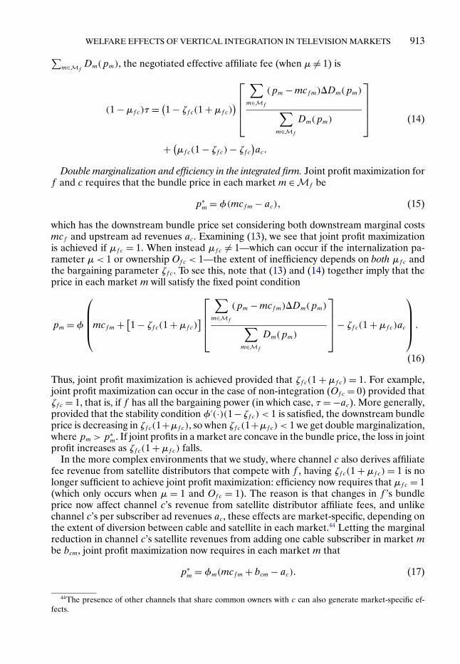
WELFARE EFFECTS OF VERTICAL INTEGRATION IN TELEVISION MARKETS 913∑m∈Mf
Dm(pm), the negotiated effective affiliate fee (when μ �= 1) is
(1 −μfc)τ = (1 − ζfc(1 +μfc)
)⎡⎢⎢⎢⎣
∑m∈Mf
(pm − mcfm)�Dm(pm)
∑m∈Mf
Dm(pm)
⎤⎥⎥⎥⎦
+ (μfc(1 − ζfc)− ζfc
)ac�
(14)
Double marginalization and efficiency in the integrated firm. Joint profit maximization forf and c requires that the bundle price in each market m ∈Mf be
p∗m = φ(mcfm − ac)� (15)
which has the downstream bundle price set considering both downstream marginal costsmcf and upstream ad revenues ac . Examining (13), we see that joint profit maximizationis achieved if μfc = 1. When instead μfc �= 1—which can occur if the internalization pa-rameter μ< 1 or ownership Ofc < 1—the extent of inefficiency depends on both μfc andthe bargaining parameter ζfc . To see this, note that (13) and (14) together imply that theprice in each market m will satisfy the fixed point condition
pm =φ
⎛⎜⎜⎜⎝mcfm + [
1 − ζfc(1 +μfc)]⎡⎢⎢⎢⎣
∑m∈Mf
(pm − mcfm)�Dm(pm)
∑m∈Mf
Dm(pm)
⎤⎥⎥⎥⎦− ζfc(1 +μfc)ac
⎞⎟⎟⎟⎠ �
(16)
Thus, joint profit maximization is achieved provided that ζfc(1 + μfc) = 1. For example,joint profit maximization can occur in the case of non-integration (Ofc = 0) provided thatζfc = 1, that is, if f has all the bargaining power (in which case, τ = −ac). More generally,provided that the stability condition φ′(·)(1−ζfc) < 1 is satisfied, the downstream bundleprice is decreasing in ζfc(1+μfc), so when ζfc(1+μfc) < 1 we get double marginalization,where pm > p∗
m. If joint profits in a market are concave in the bundle price, the loss in jointprofit increases as ζfc(1 +μfc) falls.
In the more complex environments that we study, where channel c also derives affiliatefee revenue from satellite distributors that compete with f , having ζfc(1 +μfc) = 1 is nolonger sufficient to achieve joint profit maximization: efficiency now requires that μfc = 1(which only occurs when μ = 1 and Ofc = 1). The reason is that changes in f ’s bundleprice now affect channel c’s revenue from satellite distributor affiliate fees, and unlikechannel c’s per subscriber ad revenues ac , these effects are market-specific, depending onthe extent of diversion between cable and satellite in each market.44 Letting the marginalreduction in channel c’s satellite revenues from adding one cable subscriber in market mbe bcm, joint profit maximization now requires in each market m that
p∗m =φm(mcfm + bcm − ac)� (17)
44The presence of other channels that share common owners with c can also generate market-specific ef-fects.

914 CRAWFORD, LEE, WHINSTON, AND YURUKOGLU
In contrast, a similar derivation to that above shows that when ζfc(1 +μfc)= 1, the pricein market m will instead be
pm =φ
⎛⎜⎜⎜⎝mcfm + (1 −μfc)
⎡⎢⎢⎢⎣
∑m∈Mf
(bcm − ac)Dm(pm)
∑m∈Mf
Dm(pm)
⎤⎥⎥⎥⎦+μfc(bcm − ac)
⎞⎟⎟⎟⎠ � (18)
which generally equals the joint profit-maximizing price only if μfc = 1.45
4. ESTIMATION AND IDENTIFICATION
In this section, we discuss the estimation of our model’s parameters and how they areidentified (given our modeling assumptions) from patterns in the data. We estimate all ofour parameters jointly in a single step; however, for exposition, we discuss our estimationprocedure in two steps:
1. We estimate θ ≡ {θ1�θ2�θ3}, where:(a) θ1 ≡ {ρ�ν�γd�γb}, where ρ ≡ {ρ0
c� ρ1c}∀c and ν ≡ {νS� νNS}, determines household
viewership decisions by governing the distribution of γict , how fast marginal utilities fromviewership decay, and the viewership utility reductions due to black-outs and distance toteams’ stadiums;
(b) θ2 ≡ {βv�βx�ρsat�α}, where ρsat ≡ {ρsatDirecTV�ρ
satDish}, determines household distribu-
tor choice;(c) θ3 ≡ {μ�ζI� ζE�σ2
ω} are parameters that affect firm incentives when pricing, bar-gaining, and determining carriage of channels. Recall that the parameter μ governs theextent to which integrated channels and distributors internalize profits across upstreamand downstream units. Finally, σ2
ω is the variance of an error term that influences MVPDs’carriage decisions in a manner that we discuss below.
2. We estimate {λPhilR �λSD
R }, representing separate lower bounds for our rival foreclo-sure parameter in each of the markets in which RSNs took advantage of the terrestrialloophole (i.e., Philadelphia and San Diego).To capture the impact of program access rules, we assume that λR = 0 in non-loopholemarkets. That is, we assume that the program access rules effectively require integratedfirms to ignore any foreclosure incentives in dealing with non-integrated rivals.46
Our estimation procedure conditions on the ownership structures of firms that are ob-served in the data. We maintain the assumption that the integration status of a channel ordistributor does not directly affect viewership utility or distributor demand, and is not cor-related with either measurement error (e.g., in affiliate fees or markups) or market-levelprofit disturbances considered by firms when bargaining or making pricing or carriage
45Note that, consistent with our discussion above, (18) does yield a joint profit-maximizing price when bcm
is the same for all m, or when f is only active in a single market.46We take this approach as a simple approximation to capture the effects of program access rules for both
estimation and counterfactual simulation. In practice in markets subject to program access rules, an integratedchannel could attempt to deny access to a rival distributor at the risk of triggering a binding arbitration processin which the negotiated affiliate fees with other distributors might be used to determine the arbitrated price.Explicitly modeling this process is beyond the scope of the current analysis, and we leverage the assumptionthat λR = 0 when PARs are enforced for tractability. Furthermore, we do not attempt to estimate a value ofλR ≥ 0 in markets where program access rules are in effect given the absence of variation in the data that webelieve would allow us to identify such a parameter.

WELFARE EFFECTS OF VERTICAL INTEGRATION IN TELEVISION MARKETS 915
decisions.47 If these assumptions are violated, then this paper’s predictions for the effectsof vertical integration may be biased as these predictions would not account for unob-servable factors that led to observed ownership structures. For example, if a channel anddistributor are integrated for reasons outside our model (or in anticipation of positiveprofit shocks), then counterfactually demerging that pair may understate the benefits ofintegration. Likewise, if a channel and distributor are not integrated because of unmod-eled costs of integration, counterfactually merging them would overstate the benefits ofintegration.
4.1. Estimation of Parameters θ1�θ2�θ3
4.1.1. Moments Used in Estimation
We estimate the model parameters via GMM, using the following moments.
Household Viewership. For every RSN and 38 national channels in each year, we usethe difference between the following viewership moments observed in the data and pre-dicted by the model:48
1. summing across markets, the mean viewership for each channel-year;2. summing across markets, the number of households with zero viewership for each
channel-year.49
Household Distributor Choice. For every year and market, we assume that the unob-servable characteristic for each distributor’s bundle is orthogonal to a vector of instru-ments: that is, E[ξfmt(θ)Zmt] = 0, where the expectation is taken across all markets, firms,and years. For Zmt , we include: firm-state and year dummy variables xfmt ; the maximumfraction of teams carried by the relevant RSNs in the market that are not blacked out (toinstrument for bundle utility v∗
fmt); and the satellite tax within the market, interacted withan indicator for whether the bundle is offered by a cable or satellite distributor (to instru-ment for bundle prices pfmt).50 We recover ξfmt(θ) using the standard Berry, Levinsohn,and Pakes (1995) inversion to match observed and predicted market shares (at each f�m,and t).
Distributor Bargaining, Pricing, and Carriage. First, for any θ, the vector of affiliatefees {τfct} and bundle-specific marginal costs {mcfmt} can be directly computed using theoptimal pricing and bargaining conditions given by (5) and (10) (see Appendix S.B.2 of theSupplemental Material for further details). We use these predicted values of {mcfmt(θ)}and {τfct(θ)} in constructing the next set of moments which we form using only 2007 dataand values:
47This does not rule out the possibility that integrated channels may differ in quality from non-integratedchannels (e.g., have different values of ρc), as we estimate time varying channel taste parameters.
48To avoid re-solving the viewership problem for every household for every evaluation of a candidate pa-rameter vector, we follow the importance sampling approach of Ackerberg (2009). See Appendix S.B.3 of theSupplemental Material for further details.
49The MRI/Simmons data provide an estimate of the probability that a channel is never watched for na-tional channels. We regress this probability on viewership, and use the estimated relationship to predict theprobability that an RSN is never watched.
50The satellite tax changes that we use, by state year and percentage increase, are: CT 2003, 5%; FL 2002,10%; KY 2006, 5%; MA 2009, 5%; NC 2003, 7%; OH 2003, 6%; and UT 2003, 5%. We discuss these instru-ments further in Section 5.2 and in footnote 67.

916 CRAWFORD, LEE, WHINSTON, AND YURUKOGLU
1. Average affiliate fees: For each RSN active in 2007 and four national channels(ABC Family, ESPN, TNT, and USA), we minimize the difference between the model’spredicted average affiliate fees across MVPDs and observed average affiliate fees:Ef [τfct(θ)] − τo
ct (where variables with an o superscript denote values of those objectsthat are observed in the data). We weight estimated affiliate fees by national MVPD mar-ket shares conditional on observed carriage of the channel to approximate expectationsacross MVPDs.
Deviations in these and the next set of moments for implied markups reflect both mea-surement error in the data and sampling error, as our predictions are computed using asubset of U.S. markets.
2. Implied markups: For each distributor f ∈ {Comcast�DirecTV �Dish}, we minimizethe difference between the model’s predicted MVPD price-cost margin and those ob-served in the data: Em[(po
fmt − mcfmt(θ))/pofmt] − markupo
f t .3. RSN carriage: Equation (6) implies that every cable distributor f chooses the opti-
mal set of channels (from among those with which it has agreements) to include in eachmarket m’s bundle. We assume that distributor f ’s true per household profits (not persubscriber) in market m are given by π̃M
fmt(·), where
π̃Mfmt(Bmt� ·)≡ [
πMfmt(Bmt� ·)−ωfmt(Bfmt)
]� (19)
and πMfmt(Bmt� ·) represents our (the econometrician’s) estimate of a firm’s per household
profits. The term ωfmt(Bfmt) represents a mean-zero i.i.d. bundle-distributor-market-timespecific disturbance; we assume that ωfmt(·)∼N(0�σ2
ω).51
If channel c has negotiated an agreement with some firm f (i.e., f carries c on itsbundles in some non-empty set of markets), then firm f ’s optimal carriage decision givenby (6) implies that([
�fcπMfmt(Bmt ∪ f c� ·)]− [
�fcωfmt(Bfmt ∪ f c� ·)]) ≥ 0 ∀m : c ∈ Bfmt�([�fcπ
Mfmt(Bmt ∪ f c� ·)]− [
�fcωfmt(Bfmt ∪ f c� ·)]) ≤ 0 ∀m : c /∈ Bfmt�(20)
where [�fcπMfmt(Bmt� ·)] ≡ πM
fmt(Bmt� ·)−πMfmt(Bmt \ f c� ·), [�fcωfmt(Bfmt)] ≡ωfmt(Bfmt)−
ωfmt(Bfmt \ f c), and Bmt ∪ f c denotes the set of all bundles Bmt where c is added tobundle f .52 That is, these inequalities imply that in any market in which c is carried by f , fobtains higher profits from carrying than by dropping c (holding fixed prices and carriagedecisions of other firms); similarly, in any market where c is not carried, f obtains higherprofits from not carrying than by carrying c.
Given our assumptions on the distribution of ωfmt(·), it follows that
Pr(c ∈ Bfmt)= �([�fcπ
Mfmt(Bmt ∪ f c� ·)]/(2σω)
)� (21)
where � is the standard normal cumulative distribution function.We construct several moments based on the model’s predicted carriage probabilities.
First, we construct moments based on indirect inference (cf. Gouriéroux and Monfort(1996)) that match the predicted to observed relationship between carriage of a relevant
51We interpret ωfmt(·) as the difference between our estimated profits and those used by a local systemoperator when determining carriage decisions; we assume that these disturbances are not accounted for by adistributor when pricing or bargaining with channels.
52In cases where c ∈ Bfmt , this definition implies that Bmt ∪ f c = Bmt .

WELFARE EFFECTS OF VERTICAL INTEGRATION IN TELEVISION MARKETS 917
RSN by a system and (i) the ownership share of the RSN by the system’s MVPD, (ii) thedistance of the system to the RSN’s teams’ stadiums, and (iii) the fraction of teams on theRSN that are not blacked out. Table I presents the results of a linear probability regressionpredicting whether a cable system carries a relevant RSN in our data. We find that carriageof an RSN by a cable system is increasing with the share of the RSN owned by the system’sMVPD, and decreasing in the distance between the system and the RSN’s teams’ stadiumsand in the fraction of teams that are blacked out. We perform the same regression usingthe predicted carriage probabilities from our model, and match the estimated coefficientsfor vertical integration, distance, and the fraction of teams not blacked out from thisregression to the coefficients in specification (4) in Table I.53
Second, we calculate the probability that an RSN is carried by a cable distributor in arelevant market, and match the probability that is observed in the data to that predictedby our model via (21).54 Third, we set ∂Lcarriage/∂σω = 0, where Lcarriage is the predicted log-likelihood of the observed market-level RSN carriage decisions by cable MVPDs, givenby
Lcarriage =∑c∈CR
t
∑fm:c∈Af t
(1{c∈Bfmt } × log Pr(c ∈ Bfmt)+ 1{c /∈Bfmt } × log Pr(c /∈ Bfmt)
)�
where CRt denotes the set of RSNs, and Af t are the set of channels available to
MVPD f .
TABLE I
REGRESSION OF RSN CARRIAGE ON INTEGRATION STATUS, DISTANCE, AND BLACKOUT PERCENTAGEa
(1) (2) (3) (4)
VI Ownership Share 0.404*** 0.435*** 0.293*** 0.171**(0.0674) (0.0837) (0.110) (0.0852)
% Teams Not Blacked Out 0.412*** 0.399*** 0.429*** 0.477***(0.0494) (0.0586) (0.109) (0.107)
Avg. Distance to RSN’s Stadiums −0.559*** −0.630*** −0.838*** −0.795***(103 mi) (0.100) (0.117) (0.238) (0.284)
Years 2000–2010 2007 2007 2007
Systems All Systems All Systems Has P Q Has P QHas Deal No No No YesObservations 154,121 12,246 1,132 1,052R-squared 0.615 0.616 0.670 0.639
aLinear probability regression where the dependent variable is whether a cable system carries an RSN in a relevant market in 2007.Specifications differ by sample used, where “Has P Q” restricts attention to systems for which price and quantity data are available,and “Has Deal” restricts attention to system-RSN pairs where the MVPD has a deal with the RSN (i.e., carries the RSN on at leastone other system). All specifications use DMA, RSN, and (when appropriate) year fixed effects. Inclusion of system demographiccontrols (race, population density, average income, household ownership) did not appreciably change point estimates. ***p < 0�01,**p< 0�05, *p< 0�1. Standard errors are reported in parentheses, and are clustered by DMA.
53We focus on the “Has Deal” specification as our model does not predict the probability of carriage for asystem if the MVPD and channel do not have a deal.
54For example, if there are only two RSNs A and B, and A is carried on cable in 30/40 of A’s relevantmarkets, and B is carried on cable in 25/60 of B’s relevant markets, the probability that an RSN is carried bya cable distributor in a relevant market is 0�55.

918 CRAWFORD, LEE, WHINSTON, AND YURUKOGLU
4.1.2. Identification
We now provide a discussion of variation in the data that help identify the parametersof our model (given the assumptions and moment restrictions that we employ).
Viewership and Distributor Choice Parameters (θ1, θ2). We believe that our estimate ofρ, the parameters that govern the distribution of channel tastes, is determined primarilyby viewing behavior: that is, channels watched by a larger fraction of households will tendto have higher values of ρ0
c (the probability that a channel delivers positive utility), andthose that, conditional upon being watched, are watched more often will tend to havehigher values of ρ1
c (the mean of the taste distribution). Since we do not possess ratingsfor RSNs at the market level, we believe black-out and distance parameters (γb and γd)are determined from other sources; we defer discussion of these parameters until the endof this subsection.
We believe that variation in bundle market shares as observed bundle characteris-tics and prices change is the primary source of information about parameters governinghousehold bundle choice (α, βx, and βv). Table A.I summarizes the variation in pricesand channel carriage across markets. State satellite taxes are used as an instrument forprice, and the fraction of blacked-out teams on RSNs in each relevant market is used as aninstrument for viewership utility (as firms may respond to local demand shocks when de-termining carriage). We believe that observed cable and satellite pricing margins providethe main source of identification for satellite preference heterogeneity (ρsat).55
We supplement bundle market share variation with observed average affiliate fees foreach channel. Our model predicts that a channel obtains higher affiliate fees if its pres-ence has a greater impact on households’ viewership utility when determining bundlechoice (see (2)), as this implies that the channel generates larger gains from trade withdistributors. Thus, observed affiliate fees provide information regarding the distributionof channel tastes and their scaling into viewership utility. In particular, we believe that theobserved relationship between affiliate fees and ratings is the primary source of informa-tion for our “decay” parameters (νS
c for sports channels and νNSc for non-sports channels).
Our choice to allow different values of decay parameters for sports and non-sports chan-nels is motivated by the data, illustrated in Figure 3. Sports channels have consistentlyhigher negotiated affiliate fees than non-sports channels with similar ratings; our modelis able to match this pattern by attributing a higher initial utility γic and a higher decayrate νS to a sports channel that has the same ratings as a non-sports channel.56
Bargaining, Pricing, and Carriage Parameters (θ3). The Nash bargaining parameters{ζE� ζI} relate negotiated affiliate fees to distributor and channel gains from trade. If theexternal Nash bargaining parameter ζE = 0 (so that distributors obtain no surplus whennegotiating with a non-integrated channel), the bargaining first-order conditions given by(11) imply that affiliate fees between any distributor and non-integrated channel would
55Under a standard logit demand system without preference heterogeneity, there is a strict relationshipbetween product market shares and price elasticities; in these models, allowing for product-level preferenceheterogeneity can assist in rationalizing larger observed markups by reducing implied price elasticities for givenmarket shares.
56For computational reasons, during estimation we restrict νS to lie on a discrete grid while allowing all otherparameters to vary freely; see Appendix S.B.3 of the Supplemental Material for further details and robustnesstests. See also the discussion in the appendix of Crawford and Yurukoglu (2012) which examines a variant ofthis model using Monte Carlo simulation.

WELFARE EFFECTS OF VERTICAL INTEGRATION IN TELEVISION MARKETS 919
FIGURE 3.—Negotiated monthly affiliate fees and viewership ratings.
be determined solely by the distributor’s gains from trade; fees would not be affectedby advertising revenues or factors entering solely the channel’s gains from trade. Thus,controlling for viewership, we believe that the extent to which average affiliate fees fornon-integrated channels vary with advertising revenues (and the estimated joint gainsfrom trade with distributors) provides information about the value of ζE .
Next, although the internalization parameter μ enters into the computation of severalmoments (including any moment based on affiliate fees or marginal costs), we expect thatits value is primarily determined by our RSN Carriage moments and the higher observedcarriage rates between integrated distributors and channels (captured in the regressionsin Table I): as μ increases (holding all other parameters fixed), our model predicts thatdistributors have a greater incentive to carry an integrated channel for a fixed contributionof the channel to downstream profits. We believe that black-out and distance parameters,γb�γd , are determined in a similar fashion to μ. In addition, given μ and ζE , the levelof average affiliate fees for integrated channels should then provide information aboutthe value of the internal Nash bargaining parameter ζI . While the internally negotiatedaffiliate fee between an integrated distributor and channel is not directly observed, it canbe recovered from the channel’s average affiliate fees across all distributors (which isobserved) and its average affiliate fee from non-integrated distributors only (which is afunction of μ�ζE , and the channel’s gains from trade from those distributors).
An example of the variation in the data that we leverage is illustrated in Figure 4, whichpresents the integrated and non-integrated carriage of a Comcast integrated RSN in threedifferent regions of the United States. In these regions, cable systems in markets close tothe RSN’s teams’ stadiums almost always carry the RSN; systems far away most often donot. However, in markets located a moderate distance away, these RSNs are much morelikely to be carried on Comcast-owned systems than on non-integrated systems.57 These
57For example, in Figure 4(a), all Comcast systems in northern Vermont carry CSN New England (blackdots), whereas most non-Comcast systems (gray dots for systems that carry the RSN, and gray X’s for thosethat do not) do not carry CSN New England. In Figures 4(b) and 4(c), non-carriage by non-Comcast systemsoccurs much closer to the RSN’s teams’ stadiums than for Comcast systems: there is a higher ratio of gray X’sto gray dots near Washington, D.C. and Chicago than of black X’s (non-carriage by Comcast systems) to blackdots.
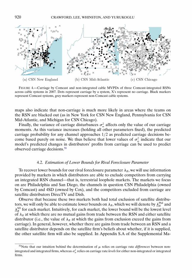
920 CRAWFORD, LEE, WHINSTON, AND YURUKOGLU
FIGURE 4.—Carriage by Comcast and non-integrated cable MVPDs of three Comcast-integrated RSNsacross cable systems in 2007. Dots represent carriage by a system, X’s represent no carriage. Black markersrepresent Comcast systems, grey markers represent non-Comcast cable systems.
maps also indicate that non-carriage is much more likely in areas where the teams onthe RSN are blacked out (as in New York for CSN New England, Pennsylvania for CSNMid-Atlantic, and Michigan for CSN Chicago).
Finally, the variance of carriage disturbances σ2ω affects only the value of our carriage
moments. As this variance increases (holding all other parameters fixed), the predictedcarriage probability for any channel approaches 1/2 as predicted carriage decisions be-come based purely on noise. We thus believe that lower values of σ2
ω indicate that ourmodel’s predicted changes in distributors’ profits from carriage can be used to predictobserved carriage decisions.58
4.2. Estimation of Lower Bounds for Rival Foreclosure Parameter
To recover lower bounds for our rival foreclosure parameter λR, we will use informationprovided by markets in which distributors are able to exclude competitors from carryingan integrated RSN channel—that is, terrestrial loophole markets. The markets we focuson are Philadelphia and San Diego, the channels in question CSN Philadelphia (ownedby Comcast) and 4SD (owned by Cox), and the competitors excluded from carriage aresatellite distributors DirecTV and Dish.
Observe that because these two markets both had total exclusion of satellite distribu-tors, we will only be able to estimate lower bounds on λR, which we will denote by λPhil
R andλSDR for each market. Intuitively, for each market, the lower bound will be the lowest level
of λR at which there are no mutual gains from trade between the RSN and either satellitedistributor (i.e., the value of λR at which the gains from exclusion exceed the gains fromcarriage). In general, however, whether there are gains from trade between an RSN and asatellite distributor depends on the satellite firm’s beliefs about whether, if it is supplied,the other satellite firm will also be supplied. In Appendix S.A of the Supplemental Ma-
58Note that our intuition behind the determination of μ relies on carriage rate differences between non-integrated and integrated firms, whereas σ2
ω relies on carriage rate levels for either non-integrated or integratedfirms.

WELFARE EFFECTS OF VERTICAL INTEGRATION IN TELEVISION MARKETS 921
terial, we show that a necessary condition for non-supply, regardless of the satellite firm’sbeliefs, is that the joint profit of the RSN c and the two satellite firms g and g′ is reducedwhen both satellite firms have access to the RSN, which can be stated as∑
m∈Mc
[[�gc�g′cΠ
Mgmt
({Bo
mt ∪{gc�g′c
}}�po
mt� τ̃; μ̂)] � � �+ [
�gc�g′cΠMg′mt
({Bo
mt ∪{gc�g′c
}}�po
mt� τ̃; μ̂)] � � �+ [
�gc�g′cΠCcmt
({Bo
mt ∪{gc�g′c
}}�po
mt� τ̃; μ̂�λR
)]]≤ 0�
(22)
where Mc represents the set of c’s relevant markets. The left-hand side of (22), whichwe refer to as the “three-party surplus,” represents g, g′, and c’s joint gains from tradefrom both g and g′ being supplied with channel c and carrying the channel in all of c’srelevant markets, and τ̃ equals the predicted values of affiliate fees τ̂(·) except that τ̃gct =τ̃g′ct = 0.59
For each of the loophole-market cable-integrated RSNs that do not contract with thesatellite distributors (CSN Philadelphia and 4SD), we estimate the corresponding lowerbound that holds for any beliefs held by a satellite firm about whether the RSN will alsobe supplied to the rival satellite firm by finding the lowest value of λR that makes (22)hold.60,61
Incentives for Exclusion
It is instructive at this point to discuss the competing forces that would induce a cableprovider to withhold its integrated RSN from a satellite provider. This is equivalent tounderstanding why the gains created when satellite distributors are supplied with the RSNmay be offset by the losses incurred by the integrated cable provider.
The primary gains-from-trade contemplated when a satellite distributor g is suppliedwith the RSN are through potential market expansion effects from carriage, that is, ifconsumers who previously did not subscribe to any MVPD now would if satellite wereto carry the RSN. Each household that substitutes from the outside good to g wouldgenerate additional industry profit equal to the level of g’s margins plus any additionaladvertising revenues generated by those households watching the RSN.
The primary losses generated by supplying g with the RSN would be incurred by theRSN’s integrated cable distributor if households substituted away from the integratedcable provider to g. Although these consumers would generate profit for g, insofar ascable margins are higher than those of satellite providers (by 10+ percentage points in
59Specifically, we show that in an alternating offer bargaining game of the form studied by Collard-Wexler,Gowrisankaran, and Lee (2018), if the three-party-surplus is positive, then RSN c has a deviating pair ofoffers {τ̃gc� τ̃g′c} to both satellite distributors that both will accept regardless of their beliefs over whether, ifthey are supplied, their rival will also be supplied, and that will increase c’s profits. See Appendix S.A of theSupplemental Material for a formal derivation and discussion of the idea behind this result.
60The left-hand side of (22) is linear and decreasing in λR (see the definition of ΠCcmt(·) from (8)).
61An alternative would be to assume that when approached by the RSN to negotiate supply, a satellite firmholds the belief that the rival satellite firm will not be supplied. The approach we employ instead provides alower bound for λR that holds for any beliefs.

922 CRAWFORD, LEE, WHINSTON, AND YURUKOGLU
our data), any household that switched from cable to satellite as a result of supplyingsatellite with the RSN would reduce industry profit by this difference in margins.62
Consequently, factors that make exclusion of satellite by an integrated cable owner (forλR > 0) more likely include: (i) a smaller share of consumers that are not subscribers toany MVPD and lower advertising rates (thereby reducing the potential gains generatedby market expansion); (ii) a larger cable “footprint” (market share) in the RSN’s rele-vant market area; (iii) closer substitutability between satellite and cable distribution; and(iv) a larger differential between cable and satellite margins (all of which would exacer-bate the losses from business stealing by satellite from cable). For all such factors, lowervalues of λR (closer to 0) cause any losses incurred by the RSN’s integrated owner to beinternalized less by the RSN when bargaining with g, reducing the likelihood of exclusionoccurring.
5. RESULTS AND PARAMETER ESTIMATES
Estimates of selected key parameters of our model are reported in Table II. We dis-cuss our estimates primarily through how they influence predicted moments relating toconsumer viewership and subscription patterns, firm pricing and carriage decisions, andnegotiated agreements.
TABLE II
ESTIMATES OF KEY PARAMETERSa
Parameter Description Estimate SE
Viewership νNS Viewership Decay, Non-sports 0�59 0.00Parameters νS Viewership Decay, Sports 0�95 —θ1 γb Fraction of Teams Blacked-out −0�58 0.31
γd (103 mi) Distance −0�93 0.27
Bundle Choice α Bundle Price −1�00 0.44Parameters βv Bundle Viewership Utility 0�14 0.07θ2 ρsat
DirecTV(102) DirecTV Exponential Parameter 0�42 0.23ρsat
Dish(102) Dish Exponential Parameter 0�49 0.27
Pricing, Bargaining, σ2ω Variance of Carriage Shocks 0�00 0.00
Carriage and ζE Bargaining, External 0�28 0.03Foreclosure Parameters ζI Bargaining, Internal 0�37 0.06θ3�λR μ Internalization 0�79 0.09
μ× λPhilR Internalization & Rival Foreclosure, Philadelphia 1�11 0.14
μ× λSDR Internalization & Rival Foreclosure, San Diego 0�94 0.11
aSelected key parameters from the first and second step estimation of the full model, where parameter νS is estimated separatelyvia a grid search (see Appendix S.B.3 of the Supplemental Material). Additional viewership parameters contained in θ1 are reportedin Appendix Table A.IV; state-firm and year fixed effects in θ2 are not reported. Asymptotic GMM standard errors are computed usingnumerical derivatives and 1500 bootstrap draws of markets and simulated households to estimate the variance-covariance matrix ofthe moments. Estimates and standard errors for μ× λPhil
R and μ× λSDR are for the lower bound of these parameters.
62Our timing assumptions rule out the possibility that an integrated channel contemplates the possibility ofraising the rival g’s price through “raising rivals’ cost” effects (cf. Salop and Scheffman (1983)). However, fora single cable-integrated RSN whose rivals are satellite distributors that set a single national price, this effectwould be small, as an increase in the RSN’s affiliate fee would only affect satellite distributors’ costs in a smallportion of their markets (in 2007, no single RSN served more than 10.4% of any satellite distributors’ potentialcustomers).

WELFARE EFFECTS OF VERTICAL INTEGRATION IN TELEVISION MARKETS 923
5.1. Viewership Parameters
The willingness-to-pay (WTP) for each channel can be derived by computing the con-tribution of a given channel to bundle utility for each household (v∗
ijt in (2)), multiplyingit by our estimates of parameters βv/α to convert it into dollars, and averaging acrosshouseholds (as households have different tastes (γict) for each channel, which are dis-tributed according to parameters ρ).63 We report estimated values of these parametersand WTPs in 2007 for all channels in Appendix Table A.IV. We also depict the distri-bution of household WTPs for nine national channels, conditional on being positive, inFigure 5(a), with the fraction of households with positive valuations listed for each chan-nel. Although most national channels have average WTP values below $1 per month (andother than sports channel ESPN, none exceed $2), the pattern is very different for RSNs:none are predicted to have average WTP values less than $1 per month, and over 70%are greater than $2.
Our estimates of the RSN distance-decay parameter γd and black-out parameter γb arenegative, and imply that consumers derive less utility from watching an RSN both (i) thefurther they are from the teams carried on the RSN, and (ii) the greater the fraction ofteams that are blacked out. We predict that increasing the average distance of a house-hold from an RSN’s teams’ stadiums from 0 to 100 miles reduces that household’s valueof the channel by approximately 9%.64 Figure 5(b) illustrates this pattern, and plots thepredicted average WTP in 2007 for four different RSNs as the distance from a house-hold to an RSN’s teams’ stadiums increases.65 Similarly, we predict that subjecting half ofthe teams that an RSN normally broadcasts to black-out restrictions reduces consumers’valuation of the channel by 25%.
Finally, we estimate νNS to be different than νS. The lower estimated value of νNS im-plies that consumers’ marginal utility from watching non-sports channels falls more slowlythan for sports channels; in turn, this implies that consumers derive higher utility fromsports channels than non-sports channels if they choose to spend the same amount oftime spent watching each. Our model thus predicts that sports channels receive highernegotiated affiliate fees for the same viewership ratings, as depicted in Figure 5(c) for theyear 2007.
5.2. Distributor Choice Parameters
All reported coefficients in θ2 are statistically significant at the 5% level, and have theexpected sign: consumers negatively respond to price (α), and positively respond to theindirect utility they receive from a bundle’s channels (βv).
At the top of Table III, we report the average own- and cross-price elasticities that arepredicted by our model. Demand for the average cable system is more inelastic (−1�7)
63We compute the average WTP for channels relative to a synthetic bundle that includes every nationalchannel carried by at least 60% of systems in 2007, and by using 20,000 simulated households. When computingthe WTP for an RSN c, we add the RSN to the synthetic bundle and use the average values of bict and dic acrossall markets that carry the RSN.
64As distance is measured in thousands of miles, being further away by 100 miles scales utility byexp(γ̂d × 0�1).
65Each point in Figure 5(b) corresponds to a market in which the RSN is carried in 2007, and the WTP foreach market is computed by averaging over 160 simulated households per market using that market’s value ofbict and dic .

924 CRAWFORD, LEE, WHINSTON, AND YURUKOGLU
FIGURE 5.—Predicted willingness-to-pay (WTP) for channels (2007 values).
than for satellite (−2�9 and −4�2), which is consistent with higher cable market shares andmargins that are both observed in the data and predicted by our model.66 Estimated valuesof ρsat
DirecTV and ρsatDish indicate consumers have substantial heterogeneity in their valuation
66Our estimates can be compared to Goolsbee and Petrin (2004), who estimated household demand forsatellite, basic cable, premium cable, and local antenna using 2001 data; they obtained an expanded basic cableown-price elasticity of −1�5, and an overall satellite own-price elasticity of −2�5. They did not observe cross-sectional variation in prices for satellite distributors, and relied on Slutsky symmetry to identify satellite priceelasticities. Our estimated own-price elasticity for cable is similar, and the overall satellite own-price elasticityimplied by our own- and cross-price elasticity estimates for DirecTV and Dish, computed at average marketshares during our sample period (see Table A.I), is −3�2.

WELFARE EFFECTS OF VERTICAL INTEGRATION IN TELEVISION MARKETS 925
TABLE III
ELASTICITIES AND MARGINSa
Elasticity of Row With Respect toPrice of Column: Cable DirecTV Dish
Cable −1.69 0.30 0.19DirecTV 2.16 −2.90 0.13Dish 3.18 0.22 −4.15Outside Option 5.52 0.26 0.16
Predicted Margins
Mean Comcast Margin 0.66Mean DirecTV Margin 0.48Mean Dish Margin 0.45
Logit Demand Price Coefficients
OLS Logit Price Coefficient −0.004** (0.002)IV Logit Price Coefficient −0.080*** (0.025)
Semi-Elasticity of Row With Respect toRemoval of ESPN From column: Cable DirecTV Dish
Cable −18.90 3.86 2.36DirecTV 54.82 −19.52 1.11Dish 51.16 1.85 −19.67Outside Option 17.27 0.22 0.14
aThis table reports predicted mean price elasticities, predicted margins for Comcast and thetwo satellite distributors, the estimated price coefficient from a logit demand regression without(OLS) and with (IV) the use of price instruments (where standard errors clustered at marketlevel), and semi-elasticities from dropping the national channel ESPN. For logit demand esti-mates, **, *** represent significance at the 5% and 1% levels.
for satellite bundles (a standard deviation of approximately $40 per month); as discussedearlier, such heterogeneity assists the model in matching observed Comcast, DirecTV, andDish price-cost margins. The implied average predicted margins are given in the secondpanel of Table III.
To illustrate the efficacy of instruments described in the previous section (which in-clude satellite taxes), the third panel of Table III reports the results from a logit demandregression.67 Instrumenting for price yields a 22 times larger estimated price coefficient,
67For 20,784 firm-market-year bundles, the dependent variable is the log of the ratio of market shares for thebundle to the outside option, and the OLS regressors are firm-state and year fixed effects, channel fixed effectsfor all channels contained in the bundle, and price. The excluded instruments for price in the IV regression arethe satellite tax within the market interacted with an indicator for whether the bundle is offered by a satelliteor cable distributor, and the maximum fraction of teams not blacked out within the market across all RSNsfor which the market is relevant. The F -statistic on the excluded instruments in the first stage regression ofprice is 425.4; the t-statistic for satellite taxes interacted with a satellite distributor indicator in the first stageprice regression is 35; and the R2 from the regression is 0�52. Additionally, an important input into distributordemand elasticities with respect to carriage is the coefficient on mean viewership utility in the distributor choiceutility equation in (2). The first stage regression of v∗
fmt on the same set of instruments for price results in anF -statistic on the excluded instruments of 389.4; the t-statistic for the maximum fraction of teams not blackedout is 33; and the R2 from the regression is 0�56.

926 CRAWFORD, LEE, WHINSTON, AND YURUKOGLU
consistent with the presence of a positive correlation between prices and unobservablebundle characteristics.
The bottom panel of Table III reports the semi-elasticity for MVPDs and the outsideoption given the removal of ESPN from each type of distributor (cable or either of the twosatellite providers). For example, the removal of ESPN from DirecTV’s bundles impliesthat its own market share would fall by 19.5%, while those for cable and Dish wouldincrease by 3.9% and 1.8%, respectively. This implies that for every 1,000 households thatwould leave DirecTV if it lost access to ESPN, 920 would substitute to cable, 67 wouldsubstitute to Dish, and 13 would go to the outside option. These types of diversion figures,and in particular those to cable, play a central role in the incentives of an integrated cableprovider to deny access to a rival satellite distributor.
5.3. Pricing, Bargaining, Carriage, and Foreclosure Parameters
We now discuss the parameters contained in θ3 which govern a firm’s pricing, bargain-ing, and carriage decisions, as well as our rival foreclosure parameter λR.
First, we estimate that the variance of firms’ bundle-market-time specific profit shocks(σ̂2
ω) is neither economically nor statistically significant. We estimate that channels cap-ture more than half of the gains from trade when bargaining, although less with integrateddistributors (ζ̂I = 0�38) than non-integrated distributors (ζ̂E = 0�28).
Our estimated value of μ indicates that firms internalize a substantial fraction, but notall, of the profits of other integrated units when making decisions. Only $0.79 of each dol-lar of profit realized by its integrated partner is internalized when an integrated MVPDmakes pricing and carriage decisions, or when integrated MVPDs and RSNs bargain witheach other. The discussion in Section 3.4.3 suggested ζfc × (1+μfc) as a (rough) measureof the alignment of downstream carriage and pricing decisions with joint profit maximiza-tion for a channel and MVPD.68 Our estimates imply that this quantity is 0�28 with non-integration, and 0�66 with a fully-integrated channel. This difference is statistically signif-icant at standard confidence levels. Moreover, we reject both μ̂= 1 and ζ̂I × (1 + μ̂) = 1,indicating that integration does not lead to full joint profit maximization.
Our estimated lower bounds for μ × λPhilR and μ × λSD
R are 1�11 and 0�94. Figure 6graphs the total three-party surplus—given by the left-hand side of (22)—between theintegrated channel and the two satellite distributors in the two loophole markets we ex-amine (Philadelphia and San Diego). We see that for values of μ × λR lower than 0�94,it is not an equilibrium for either channel to exclude both satellite distributors, as therewould be a profitable deviation, for some negotiated set of affiliate fees, for the channelto be supplied. However, for values between approximately 0�94 and 1�11, we can ratio-nalize exclusion in San Diego but not Philadelphia. Only for values of μ×λR ≥ 1�11 doesour model rationalize exclusion in both of these loophole markets. These results indicatethat integrated channels’ supply decisions vis-à-vis non-integrated rival distributors aresignificantly affected by foreclosure incentives; these weights placed on the benefits of ri-val foreclosure for the channel’s integrated distributors are not statistically significantlydifferent from 1.69
68Specifically, ζfc × (1 +μfc)= 1 would lead to joint profit-maximizing carriage and pricing decisions whenthe MVPD operates in a single market.
69Given μ̂ = 0�79, these estimates imply that λPhilR is at least 1�4 and λSD
R at least 1�3, which corresponds tothe integrated channel placing more weight on its integrated distributor’s benefits from foreclosure than thechannel and distributor place on each other’s profits when pricing, making carriage decisions, and bargaining

WELFARE EFFECTS OF VERTICAL INTEGRATION IN TELEVISION MARKETS 927
FIGURE 6.—Three-party surplus between the integrated cable MVPD, DirecTV, and Dish as a function ofμ× λR in Philadelphia and San Diego.
6. THE WELFARE EFFECTS OF VERTICAL INTEGRATION
In this section, we use our model’s estimates to examine how vertical integration affectsaffiliate fee negotiations (including whether supply occurs at all), distributors’ pricing andcarriage decisions, and—ultimately—firm and consumer welfare. We focus on 26 RSNsthat were active in 2007, 13 of which were (at least partially) integrated with a downstreamdistributor (10 with a cable MVPD, 3 with DirecTV).70 Of these integrated RSNs, two—CSN Philadelphia and 4SD—were owned by cable distributors in “loophole” markets,and were not provided to satellite.
For each of these RSNs, we simulate market outcomes for the year 2007 that wouldhave occurred in the RSN’s relevant markets under the following three integration scenar-ios: (i) Non-integration, (ii) Integration with PARs, and (iii) Integration without PARs.71
More specifically:(i) Non-Integration: In this scenario, we assume that μ = 0 and λR = 0 so that all firms
behave as if they are non-integrated (i.e., no MVPD or channel internalizes the profits ofany other unit).
(ii) Integration with PARs: In this scenario, if the RSN being examined is non-integrated in the data, we assign full ownership of the channel to the largest cable MVPDin that RSN’s relevant markets; if the RSN is integrated, we do not change its owner-ship structure. We then assume that μ is equal to our estimated value μ̂ = 0�79, but thatλR = 0: that is, we assume that integrated distributors and channels partially internalizeeach other’s profits when bargaining with each other over affilliate fees, and when theintegrated distributor is pricing and making carriage decisions, but that program access
with each other. However, we cannot reject the hypothesis that either of these values differ from 1: the 95%
confidence interval for λ̂PhilR is [0�97�1�93] and λ̂
SDR is [0�82�1�70].
70We exclude from our analysis three cable-integrated RSNs (CSN Northwest, Comcast/Charter SportsSoutheast, and Cox Sports TV) and one independent RSN (YES) that did not supply satellite providers inmarkets where PARs were in effect, as our model does not explain this exclusion.
71We simulate the equilibrium under all three scenarios for each RSN, including whichever scenario oc-curred in the data for the RSN.

928 CRAWFORD, LEE, WHINSTON, AND YURUKOGLU
rules prevent the channels from considering the benefits of foreclosure to its integrateddistributor when bargaining with rival distributors.
(iii) Integration without PARs: In our final scenario, we follow the same setup as inthe “Integration with PARs” scenario, but assume that λR = λ̂
Phil
R , the larger of our tworecovered lower bounds.72 The RSN therefore internalizes the profits of its downstreamintegrated units when bargaining with other downstream distributors, and thus may findit unprofitable to supply downstream rivals.
For each integration scenario and each RSN, we solve for a set of bundle prices, car-riage decisions, and negotiated affiliate fees that satisfy the necessary equilibrium condi-tions given by equations (5), (6), and (11). Under non-integration and integration withPARs (scenarios (i) and (ii)), we assume that all RSNs are supplied to all distributors.73
Under scenario (iii), where channels are integrated but PARs are not in effect, we alsosolve for the RSN’s equilibrium supply decision. To determine whether or not each rivaldistributor is supplied with the channel, we test which supply outcomes (e.g., if a cableintegrated RSN supplies both, neither, or either one of the two satellite distributors) areconsistent with equilibrium.74
In our main counterfactual results, we assume that a change in ownership for a singleRSN does not cause national satellite prices to adjust, and we thus hold satellite pricesfixed at observed levels. In Section 6.3, we also examine counterfactuals under the alter-native assumption that satellite prices are determined at the DMA level, and may adjustacross our integration scenarios. Further computational and implementation details areprovided in Appendix S.B.4 of the Supplemental Material.
6.1. Potential Effects
Before proceeding, it is instructive to highlight the effects of vertical integration that arecaptured by our model and that we attempt to quantify. Our model emphasizes three main
72The value of λR must be at least λ̂PhilR to rationalize the non-supply of the satellite distributors that we
observe in both Philadelphia and San Diego. If λR > λ̂PhilR , foreclosure incentives would be larger than those
considered here; we explore the effects of larger values of λR in Section 6.3.73Aside from the two loophole RSNs, all other RSNs in our counterfactuals were provided to all distributors
in 2007.74At the set of affiliate fees, prices, and carriage decisions that satisfy the necessary equilibrium conditions
under each potential supply outcome, for each cable-owned channel in scenario (iii) we test: (a) whethersupplying both satellite providers is an equilibrium by examining if there are positive bilateral gains from tradebetween the RSN and each satellite provider given that the other satellite provider is supplied; (b) whethersupplying only one satellite distributor is an equilibrium by examining if there are positive gains from tradebetween the RSN and the supplied satellite distributor given that the other satellite provider is not supplied,and if there are no bilateral gains from trade between the RSN and the non-supplied satellite distributorgiven that the other satellite provider is supplied; and (c) whether supplying neither satellite distributor is anequilibrium by examining if the three-party-surplus given by the left-hand side of (22) is negative. For all RSNsbut two, exactly one supply outcome was robust to these tests. For two RSNs, exactly two supply outcomessatisfied these tests: for CSN Philadelphia, they were the non-supply of both satellite distributors and thesupply of only DirecTV; for NESN, they were the non-supply of both or supply of both. We report resultsassuming that the outcome with the least supply is chosen (as this outcome maximized the integrated firms’profits given our parameter estimates). For each of the three RSNs owned by DirecTV, we determine supply byverifying that the bilateral surplus generated by the RSN’s supply of each cable MVPD in the RSN’s relevantmarkets as well as Dish Network is positive (where surpluses are computed at updated levels of affiliate fees,prices, and carriage decisions).

WELFARE EFFECTS OF VERTICAL INTEGRATION IN TELEVISION MARKETS 929
supply-side decisions: (i) negotiations over supply and affiliate fees between channels anddistributors, and both (ii) channel carriage (conditional on supply) and (iii) bundle pricingby distributors.
Suppose, then, that MVPD f integrates with RSN c, and that there is a rival MVPD g.The following effects of vertical integration are admitted in our setting:
1. Bargaining Effects and Foreclosure: When integration occurs, there are effects onboth internal and external bargaining. As discussed in Section 3.4.3, we expect the ef-fective internal affiliate fee paid by the integrated distributor f to fall when integrationoccurs: that is, our 0.79 estimated value of μ indicates that the RSN and distributor finternalize (most of) each others’ payoffs. Of course, in equilibrium, the internal affiliatefee is also affected by any changes in carriage and pricing as these can change both f andc’s gains from trade.
The effects of integration on external bargaining will depend on whether PARs are ineffect or not. When PARs are in effect, RSN c ignores any benefits to its integrated dis-tributor f ’s profits from denying access to rival distributor g, just as if c was not integrated.However, the negotiated affiliate fee to g may still be affected by changes in f ’s carriageand prices, which can affect g’s benefit from getting access to c, and by any change in theinternal affiliate fee that c receives from f (which would alter how supply of g affects c’sprofit).
Finally, when c bargains with the rival MVPD g and PARs are not in effect, c internal-izes the lost profit of its integrated downstream distributor f if g is supplied (since λR > 0).As a result, the gains-from-trade that accrue to c by supplying g are reduced from whatthey would be under either non-integration or in the presence of PARs, potentially leadingto a higher negotiated affiliate fee τgct or—if gains-from-trade are eliminated altogether—non-supply. Again, however, any induced changes in carriage and pricing can also affectnegotiated input fees.
2. Carriage Effects: When vertical integration occurs, the fact that μ is positive makesthe integrated f internalize the effects of its carriage of RSN c on c’s profit. As carriage islikely to increase c’s profit due to the increase in affiliate fees earned from f (although anoffsetting effect is that f ’s carriage of c may lower c’s affiliate fee revenues earned from gby reducing g’s market share), integration may lead f to increase carriage of RSN c. Thenet impact on carriage will also depend on equilibrium price adjustments and whetherrival distributors are still supplied with the channel.
3. Pricing Effects: As with the carriage decision, an integrated f will internalize effectsof its pricing on RSN c’s profit. This is likely to push f toward charging a lower bundleprice—that is, reducing double marginalization—as a lower price will increase f ’s marketshare, and hence the affiliate fees that c collects from f (although, as described above,there is a potentially offsetting effect from any reduced affiliate fees earned from g, as inChen (2001)). In addition, changes in carriage will have a separate effect on f ’s pricing;for example, if carriage increases, the resulting increased bundle quality is likely to pushf to increase prices in those markets where c is added to its bundle relative to what itsprices would have been absent the carriage change.
Thus, while we expect integration to increase carriage and reduce double marginaliza-tion by integrated distributors, and the absence of PARs to increase foreclosure of andaffiliate fees paid by rival distributors of integrated firms, confounding effects are presentthat may upset these expectations. Moreover, even if the directions of these effects are asexpected, their magnitudes, and their overall impacts on consumer and aggregate welfare,remain empirical questions that our counterfactual simulations aim to address.

930 CRAWFORD, LEE, WHINSTON, AND YURUKOGLU
6.2. Results
6.2.1. Individual RSN Results
As an illustration of the kinds of effects we see for individual RSNs, Table IV reportsmarket shares, channel carriage, cable prices, firm profits, and consumer and total wel-fare across our three different integration scenarios for three RSNs: CSN Philadelphia, acable-integrated RSN located in a terrestrial loophole market; MSG, a cable-integratedRSN located in a non-loophole market; and NESN, a non-integrated RSN. Below eachRSN name is the MVPD that owns the channel (or is assigned ownership under inte-gration scenarios (ii) and (iii) if the RSN is non-integrated, denoted by a * next to theassigned owner’s name), the number of households and the MVPD owner’s “footprint”(the percentage of these households that the MVPD “passes” or plausibly could serve) in
TABLE IV
SIMULATED MARKET OUTCOMES FOR SELECTED RSNSa
(i) No VI (ii) VI PARs (iii) VI No PARs(vs. No VI) (vs. No VI)
Level %�lvl %�WTP %�lvl %�WTP
Cable Integrated RSNsCSN PHIL Cable Mkt Share 0.64 0.8% 1.8%Comcast [0�62�0�65] [0�2%�2�4%] [0�6%�4�0%]Pop 4.25M Sat Mkt Share 0.18 −0.5% −10.4%Footprint 90% [0�17�0�19] [−3�3%�−0�2%] [−14�8%�−0�5%]WTP $4.99 Cable Carriage 0.95 1.6% 0.4%
[0�62�0�97] [0�0%�53�8%] [−6�2%�52�9%]Cable Prices 54.31 −0.5% 0.9%
[53�28�55�42] [−1�5%�0�9%] [−1�4%�1�8%]Foreclose: 85% Aff Fees to Sat 2.26 3.6% —
[1�00�2�64] [−9�4%�7�0%] —Cable + RSN Surplus 30.19 0.2% 0.9% 1.1% 6.5%
[14�57�32�67] [0�0%�2�4%] [0�3%�13�7%] [0�4%�3�3%] [3�0%�20�5%]Satellite Surplus 4.29 −0.9% −0.8% −2.1% −1.8%
[1�26�4�70] [−3�4%�−0�4%] [−2�4%�−0�5%] [−4�8%�−1�1%] [−4�5%�−0�9%]Consumer Welfare 31.21 0.6% 3.9% −2.9% −18.1%
[16�82�34�81] [0�2%�2�0%] [1�4%�12�7%] [−3�3%�1�5%] [−21�8%�9�9%]Total Welfare 65.69 0.3% 4.0% −1.0% −13.4%
[31�14�71�73] [0�1%�1�9%] [2�0%�25�2%] [−1�1%�1�1%] [−15�6%�14�7%]MSG Cable Mkt Share 0.63 3.3% 3.3%Cablevision [0�62�0�67] [0�3%�4�8%] [0�2%�4�7%]Pop 11.7M Sat Mkt Share 0.18 −4.3% −4.3%Footprint 42% [0�17�0�18] [−7�1%�−0�4%] [−8�1%�−0�4%]Pred WTP $2.32 Cable Carriage 0.68 10.5% 10.5%
[0�67�0�87] [−2�5%�18�5%] [−3�1%�18�5%]Cable Prices 59.40 −2.4% −2.4%
[56�80�60�81] [−3�5%�0�0%] [−3�5%�0�2%]Foreclose: 1% Aff Fees to Sat 1.22 −3.3% 22.4%
[0�42�1�28] [−5�9%�10�4%] [17�1%�53�4%]Cable + RSN Surplus 30.64 0.3% 4.4% 0.5% 6.8%
[14�61�34�12] [−0�1%�0�6%] [−1�6%�7�4%] [0�0%�1�3%] [0�4%�14�6%]Satellite Surplus 4.16 −4.2% −7.5% −5.5% −9.9%
[1�24�4�48] [−7�2%�−0�5%] [−12�1%�−0�9%] [−8�5%�−1�2%] [−14�3%�−2�4%]Consumer Welfare 33.80 3.1% 44.6% 3.0% 44.3%
[18�38�38�14] [0�3%�4�3%] [4�4%�66�3%] [−0�4%�4�3%] [−6�3%�66�0%]Total Welfare 68.60 1.4% 41.4% 1.4% 41.2%
[32�06�76�01] [0�1%�1�9%] [3�4%�60�9%] [0�1%�1�9%] [2�5%�60�7%]
(Continues)

WELFARE EFFECTS OF VERTICAL INTEGRATION IN TELEVISION MARKETS 931
TABLE IV—Continued
(i) No VI (ii) VI PARs (iii) VI No PARs(vs. No VI) (vs. No VI)
Level %�lvl %�WTP %�lvl %�WTP
Non-Integrated RSNNESN Cable Mkt Share 0.61 7.6% 9.4%*Comcast [0�59�0�65] [1�6%�11�2%] [2�7%�12�5%]Pop 5.20M Sat Mkt Share 0.13 −7.8% −22.3%Footprint 85% [0�12�0�14] [−12�6%�−1�8%] [−26�5%�−7�2%]WTP $6.91 Cable Carriage 0.92 6.2% 3.6%
[0�68�0�98] [0�0%�33�1%] [−0�5%�38�1%]Cable Prices 56.73 −4.7% −3.9%
[54�24�57�88] [−6�6%�−0�5%] [−6�0%�0�6%]Foreclose: 96% Aff Fees to Sat 3.32 3.1% —
[1�23�3�79] [−12�6%�16�9%] —Cable + RSN Surplus 28.38 0.9% 3.6% 2.0% 8.2%
[13�68�31�36] [0�1%�2�4%] [0�9%�10�6%] [0�7%�4�0%] [5�4%�16�7%]Satellite Surplus 2.96 −8.3% −3.5% −10.9% −4.7%
[0�84�3�24] [−13�2%�−1�8%] [−5�5%�−1�3%] [−13�9%�−3�0%] [−6�3%�−1�7%]Consumer Welfare 28.36 6.4% 26.5% 3.3% 13.5%
[15�54�31�97] [1�4%�10�0%] [8�2%�40�8%] [−1�7%�7�1%] [−9�0%�29�2%]Total Welfare 59.70 3.1% 26.5% 2.0% 17.0%
[29�79�65�84] [0�5%�5�1%] [7�8%�43�7%] [−0�2%�4�5%] [−2�5%�37�5%]
aScenarios (i)–(iii) correspond to the integration scenarios described at the beginning of Section 6. Beneath the RSN name is eitherthe name of the RSN’s owner (observed or, if non-integrated, assigned, which is denoted by ∗), the number of television households inthe RSN’s relevant markets, the MVPD owner’s footprint (% of households passed) in the RSN’s relevant markets, and the estimatedmean consumer WTP for the RSN. Scenario (i) reports household weighted averages over all relevant markets for each RSN, where alllevels except for market shares and cable carriage are in $/household/month. Scenarios (ii) and (iii) report changes from scenario (i),where %�lvl (respectively, %�WTP) represent changes from scenario (i) expressed as a percentage of changes in household weightedaverages of levels (respectively, estimated mean consumer WTP for the channel). Affiliate fees to satellite are reported conditionalon supply; missing values indicate foreclosure. 95% confidence intervals, constructed from 150 simulations, are reported below eachfigure; the fraction of simulations in which the RSN is predicted to foreclose at least one rival distributor under scenario (iii) is reportedlast under each RSN’s name (“Foreclose: %”). Results for all other RSNs are contained in Appendix Tables A.V–A.VII.
the RSN’s relevant markets, and the estimated mean consumer willingness-to-pay (WTP)for the RSN.
The values shown for scenario (i), corresponding to no vertical integration (“No VI”),are household weighted average levels across an RSN’s relevant markets; with the excep-tion of market shares and cable carriage, reported numbers are in dollars per householdper month. For integration scenarios (ii) and (iii), “VI PARs” and “VI No PARs” re-spectively, we report changes from non-integration scenario (i) either as a percentageof non-integration levels (denoted %�lvl) or as a percentage of the mean WTP for theRSN (denoted %�WTP). A missing value for “Aff Fees to Sat” indicates that the RSN ispredicted to be withheld from the two satellite distributors. Confidence intervals are con-structed by taking 150 draws from the joint distribution of the estimated coefficients andrecomputing the equilibrium for each draw. The fraction of the scenario (iii) draws forwhich the RSN is predicted to foreclose and not supply at least one rival distributor isalso shown last under each RSN name (“Foreclose: %”).
For each of the three RSNs shown in Table IV, vertical integration with PARs in ef-fect leads the integrated distributor to increase carriage and reduce its bundle price atour point estimates, and in each case we can reject a zero effect for at least one of thecarriage or price effects. Cable’s market share increases in each case, and satellite’s sharedecreases; as well, satellite surplus falls, consumer welfare increases, and total welfarerises (all such effects are statistically significant).

932 CRAWFORD, LEE, WHINSTON, AND YURUKOGLU
When integration occurs without PARs in effect, two of these three RSNs—CSNPhiladelphia and NESN—deny access to both rival satellite producers. Despite this ex-clusion, only for CSN Philadelphia are the point estimates for the effects of vertical inte-gration on consumer and total welfare negative, and for neither of these two RSNs canwe reject zero net consumer and total welfare effects. For the third RSN, MSG, the twosatellite distributors continue to have access to the RSN, although paying higher affiliatefees (22.4% higher according to our point estimates, and statistically significantly differ-ent from zero). For all three RSNs, vertical integration without PARs in effect lowers thesatellite distributors’ profits by between 2 and 11% (statistically significant in each case).
Results for all other RSNs are contained in Appendix Tables A.V–A.VII. Overall, theoutcomes for different RSNs display considerable heterogeneity.
6.2.2. Average Results
We now turn to the average effects of vertical integration. Table V reports market out-comes for each of the three vertical integration scenarios, averaged across RSNs andweighted by the number of households in each RSN’s relevant markets. The structureis the same as in Table IV, with the following adjustments. First, “Aff Fees to Rivals”represents the weighted average of the affiliate fees charged to the integrated MVPD’srival distributors (weighted by the number of households in each of the RSN’s relevantmarkets), conditional on the channel being supplied to those distributors. These rival dis-tributors are the two satellite distributors if the channel is cable-integrated; if instead thechannel is DirecTV-integrated, these rivals are the cable distributors in the RSN’s rel-evant markets and Dish. Second, “# Foreclosed” represents the number of RSNs thatare not provided to at least one rival distributor for the case of integration without PARsin effect (integration scenario (iii)). Third, in the rightmost two columns, we report theweighted average change in predicted outcomes between scenarios (ii) and (iii); thesechanges are expressed both as percentages of scenario (ii) levels and of an RSN’s esti-mated mean WTP, and isolate the impact of program access rules given integration. Allreported percentages are the averages of percentage changes across RSNs, weighted bythe number of households in each RSN’s relevant markets.
Efficiency Effects: Reduction of Double Marginalization and Increased Carriage. We firstfocus on the potential efficiency gains from vertical integration. These are highlighted bythe differences between integration scenario (ii) with PARs and non-integration scenario(i), reported in the second and third columns of Table V.
Across all RSNs, we predict that integration of a single RSN when PARs are in ef-fect yields on average a (statistically significant) 9.4% increase in carriage of the RSNby cable distributors.75 It also results on average in a (statistically significant) 1.2% de-crease in cable prices (corresponding to an average $0.67 reduction in the price consumerspay).76,77 As discussed in Section 6.1, pricing reductions arise primarily from the reduction
75This average includes carriage changes by cable operators for the three satellite-owned RSNs.76The values reported for scenarios (ii) and (iii) in Tables IV and V are the (household weighted) averages
of percentage changes, not the percentage change in the average levels. Thus, the average $0.67 decrease inprice that we describe here does not equal the product of the values in the first and second columns of Table V.
77Though integration of most RSNs yields less than a 1% decrease in cable prices, there are several caseswhere price decreases are larger: for example, integrating NESN with Comcast, reported in the bottom panelof Table IV, results in average cable prices falling by nearly 5% (corresponding to an average reduction inthe price consumers pay of $2.67) due to NESN’s high estimated affiliate fees to Comcast (predicted to beapproximately $4.70 per month).

WE
LFA
RE
EF
FE
CT
SO
FV
ER
TIC
AL
INT
EG
RA
TIO
NIN
TE
LE
VISIO
NM
AR
KE
TS
933
TABLE V
AVERAGE SIMULATED MARKET OUTCOMES ACROSS ALL RSNSa
(i) No VI (ii) VI PARs (iii) VI No PARs
(vs. No VI) (vs. No VI) (vs. VI PARs)
Level %�lvl %�WTP %�lvl %�WTP %�lvl %�WTP
All RSNsCable Mkt Share 0.60 2.1% 2.2% 0.1%
[0�59�0�62] [0�4%�2�6%] [0�4%�2�6%] [−0�2%�0�3%]Sat Mkt Share 0.20 −2.0% −2.7% −0.8%
[0�20�0�21] [−2�6%�−0�4%] [−4�1%�−0�8%] [−2�6%�−0�0%]Cable Carriage 0.72 9.4% 8.6% −0.7%
[0�66�0�80] [3�1%�21�5%] [0�8%�19�1%] [−4�4%�0�9%]Cable Prices 55.10 −1.2% −1.1% 0.1%
[54�25�55�90] [−1�5%�−0�1%] [−1�4%�−0�0%] [0�0%�0�3%]Aff Fees to Rivalsb 1.36 −0.7% 17.1% 18.0%
[0�54�1�45] [−3�2%�4�4%] [11�0%�28�5%] [12�1%�28�6%]Cable + RSN Surplus 23.04 0.3% 3.1% 0.6% 5.0% 0.2% 1.9%
[11�13�25�17] [0�1%�0�6%] [1�4%�5�4%] [0�2%�0�9%] [2�6%�8�1%] [0�1%�0�5%] [0�5%�4�2%]Satellite Surplus 5.10 −2.2% −4.3% −3.2% −6.0% −1.0% −1.7%
[1�56�5�51] [−3�1%�−0�5%] [−6�7%�−0�3%] [−3�9%�−1�0%] [−8�4%�−1�1%] [−1�3%�−0�4%] [−2�5%�−0�6%]Consumer Welfare 30.99 1.5% 18.0% 1.3% 16.2% −0.2% −1.7%
[16�15�34�47] [0�3%�1�8%] [5�5%�23�8%] [−0�1%�1�5%] [−1�3%�20�4%] [−0�7%�−0�1%] [−8�4%�0�0%]Total Welfare 59.13 0.7% 16.8% 0.6% 15.3% −0.1% −1.5%
[27�59�64�41] [0�1%�0�9%] [5�4%�22�2%] [0�0%�0�8%] [0�8%�18�7%] [−0�2%�−0�0%] [−6�4%�0�1%]# Foreclosed: 4/26 [0�9]
aAverage simulated market outcomes across the 26 RSNs in our analysis, weighted by the number of households in each RSN’s relevant markets. Percentages are the averages of percentagechanges across RSNs, weighted by the number of households in each RSN’s relevant markets. “# Foreclosed” reports the number of RSNs that are not provided to rival distributors under (iii) VI NoPARs. See Table IV and main text for additional details.
b“Aff Fees to Rivals” represents average affilliate fees (to the satellite MVPDs for cable-integrated RSNs, and to cable MVPDs and the rival satellite distributor for satellite-integrated RSNs)conditional on supply in each relevant scenario.

934 CRAWFORD, LEE, WHINSTON, AND YURUKOGLU
TABLE VI
WELFARE CHANGES FROM FORECLOSUREa
Percentage Change in Levels Between (ii) VI PARs and (iii) VI No PARs
%� Consumer Welfare %� Total Welfare
Are Rival Distributors Excluded −1.95*** −0.72***(0.53) (0.22)
N 3,900 3,900R2 0.52 0.52
aRegression where the dependent variable is the percentage change in either con-sumer or total welfare in levels between integration scenarios (ii) and (iii) (withand without PARs in effect). Each observation is an RSN-counterfactual simulation(26 × 150). Specifications include RSN fixed effects. Standard errors clustered at RSNlevel, and ∗∗∗ represents significance at the 1% level.
of double marginalization. However, there are offsetting effects that may mitigate down-ward pricing incentives: integrated distributors now internalize affiliate fees paid by rivalMVPDs, and (as we have noted) carriage of the RSN by cable providers increases whenthe channel is integrated (thereby increasing the utility delivered by bundles in certainmarkets). Even so, cable prices fall on average.78
We find that joint RSN and integrated cable surplus increases on average when movingfrom non-integration to integration with PARs: when a cable MVPD is integrated (andsince μ̂ is greater than 0), its pricing and carriage decisions will partially internalize RSNprofits (even if, under PARs, the channel does not act upon rival foreclosure incentives).Satellite surplus, on average across all RSNs, falls by 2.2% when RSNs are integrated withPARs in effect.79 Consumer welfare and total welfare increase by, on average, 1.5% and0.7%, respectively (18.0% and 16.8%, respectively, as percentage gains of WTP for theRSN). The change in total welfare represents an average increase of $0.43 per householdper month. Each of these changes is statistically significant.
We find that consumer welfare gains arise primarily from lower cable prices: if wehold cable prices fixed at non-integrated levels and recompute equilibrium outcomes(including carriage and affiliate fees) under integration with PARs, average consumerwelfare gains across all RSNs are 0.3%; holding fixed carriage rates at non-integratedlevels and recomputing equilibrium outcomes yields average consumer welfare gainsof 1.5%.80
Foreclosure Effects: Raising Rivals’ Costs and Exclusion. The comparison of scenarios(ii) and (iii), shown in the last two columns of Table V, provides the impact of removingPARs given that RSNs are integrated, and isolates the impact of foreclosure incentives onmarket outcomes. Allowing foreclosure is predicted to reduce both consumer and totalwelfare from the integration scenario with PARs by 0.2% and 0.1%, respectively; both are
78In fact, we find that average cable prices do not increase for any individual RSN upon integration in thepresence of PARs.
79This percentage includes both cable and satellite integration of RSNs, although it is primarily reflecting ca-ble ownership of RSNs. In Appendix Table A.VI, we report market outcomes for the three satellite-integratedRSNs.
80These partial effects, calculated from the same non-integration baseline, do not sum to the total equilib-rium effect when prices, carriage, and affiliate fees adjust.

WELFARE EFFECTS OF VERTICAL INTEGRATION IN TELEVISION MARKETS 935
TABLE VII
PROBABILITY OF EXCLUSIONa
Exclusion of Rival Distributors by Integrated RSN (Without PARs)
Footprint of Integrated Owner 0.67**(0.25)
WTP for RSN 0.07(0.05)
N 26R2 0.29
aLinear probability regression where the dependent variable iswhether rival distributors are denied access to an RSN under integra-tion scenario (iii) without PARs. Each observation is an RSN. Speci-fication includes a fixed effect for whether the RSN owner is a cableoperator. ∗∗ represents significance at the 5% level.
statistically significant, and represent average changes of 1.7% and 1.5% as a percentageof the WTP for the RSN.
The reduction in welfare from the absence of PARs stems primarily from two effects.The first occurs when an RSN is completely withheld from rival MVPDs. Though wepredict that none of the three DirecTV-owned RSNs would choose to exclude cableproviders, we predict that 3 out of the 10 RSNs integrated with a cable provider in thedata (the two loophole RSNs and CSN New England) and one previously non-integratedRSN (NESN) would exclude both satellite distributors.81 Conditional on integration oc-curring, exclusion of a rival distributor is associated with a negative change in welfare:Table VI reports results from a regression of the change in consumer and total welfarebetween VI scenarios with and without PARs on whether or not rival distributors aredenied access to the RSN. Results indicate that the exclusion of rival distributors is asso-ciated with a 1.9% and 0.7% reduction in consumer and total welfare, which roughlyequals the predicted average welfare gains from integration with PARs (%�lvl in sce-nario (ii)).
To examine when exclusion is more likely to occur, Table VII reports results from alinear probability regression of whether rival distributors are denied access to an RSNwhen PARs are not in effect; the footprint, or percentage of households in the RSN’srelevant markets that the integrated distributor can serve, is positive and statistically sig-nificant. This is consistent with the discussion in Section 4.2 (i.e., larger cable footprintsincrease the potential losses incurred by an integrated cable provider from supplying theRSN to rival satellite distributors), and reflects the fact that the cable owners for the fourRSNs that are predicted to foreclose satellite distributors all have greater than an 85%footprint.
The second effect that reduces welfare arises when an integrated RSN still supplies ri-val distributors but raises their affiliate fees, which in turn affects downstream distributorpricing and carriage. Table V indicates that affiliate fees for integrated RSNs charged torivals, conditional on supply, increase on average by a statistically significant 18.0% fromthe levels predicted when PARs are in effect.82 Even though we have assumed that satel-
81The 95% confidence interval for the number of RSNs that exclude is [0�9].82In some cases, this increase represents an increase of nearly $0.50 per month per subscriber, as with CSN
Mid-Atlantic (see Table A.V).

936 CRAWFORD, LEE, WHINSTON, AND YURUKOGLU
lite distributors do not adjust their prices in our counterfactuals, higher satellite affiliatefees can negatively harm consumer welfare by inducing the integrated cable owner to in-crease its own downstream prices or reduce its carriage. Intuitively, if a cable-integratedRSN increases its affiliate fees with satellite distributors, then the RSN’s downstream ca-ble MVPD sees a greater benefit to its integrated RSN from raising its price or reducingits carriage, which will move subscribers to the now higher-paying satellite distributors.Indeed, we find that cable prices increase, on average, by a small, but statistically sig-nificant 0.1%; carriage falls in our point estimates by 0.7%, although this change is notstatistically significant.83 Overall, removing PARs reduces satellite firms’ surplus by a sta-tistically significant 1.0% beyond the reduction caused by integration when PARs are ineffect.
Net Effects. The comparison of scenarios (iii) and (i), shown in the fourth and fifthcolumns of Table V, gives the overall net impact of integration of RSNs when PARs arenot in effect. On average across all RSNs, the efficiency effects dominate the foreclo-sure effects when examining consumer and total welfare—both increase by approximately1.3% and 0.6%, representing 15–16% of the total WTP generated by an RSN.84 This isdriven by an increase in RSN carriage (9% on average) and a reduction in cable prices(1.1%). However, satellite market shares and profits are predicted to fall by 2.7% and3.2%, respectively, when RSNs are integrated.
These average net welfare changes mask considerable heterogeneity in the point es-timates for individual RSNs. For instance, we find that foreclosure effects dominate forconsumer welfare in the terrestrial loophole markets, where 4SD and CSN Philadelphiaare predicted to exclude both satellite distributors, and reduce consumer welfare by 8–18% ($0.13–0.90) of the average WTP generated by the channel. On the other hand, av-erage net consumer welfare gains from integration for some RSNs reach approximately$1 per household per month (e.g., $1.03 for MSG and $0.94 for NESN). Looking sepa-rately at the four markets in which exclusion occurs at our point estimates, consumer andtotal welfare increase on average by small amounts (0.4% and 0.3%, respectively) and wecannot reject zero effects. In contrast, consumer and total welfare rise on average by astatistically significant 1.4% and 0.7%, respectively, in the 22 markets in which exclusiondoes not occur.85
6.2.3. “Perfect” Internalization
Although we reject that integration leads to full joint profit maximization, we havealso conducted our counterfactual simulations using our main parameter estimates underthe assumption that μ = λR = 1.86 Our findings are broadly similar: examining averagechanges between integration without PARs and no integration (scenarios (iii) and (i)),we find that consumer and total welfare gains are slightly larger than at our estimated
83This effect is discussed in Chen (2001). As a specific example, Comcast, the owner of CSN Mid-Atlantic,increases its own price of a bundle by $0.11 between scenarios (ii) and (iii) as a result of negotiating a signifi-cantly higher affiliate fee for CSN Mid-Atlantic from satellite distributors.
84On average, consumer welfare rises by $0.39 and total welfare by $ 0.38 per household per month.85Recall as well that these effects are all simulated setting the rival foreclosure parameter at its estimated
lower bound. Foreclosure would be more widespread, and vertical integration less beneficial, at larger values;see Section 6.3.
86For our simulations, we set μ= 0�99 (which ensures that internal negotiated affiliate fees are not indeter-minate when Ofct = 1; see footnote 38) and ζI = 1/(1 +μ).

WELFARE EFFECTS OF VERTICAL INTEGRATION IN TELEVISION MARKETS 937
values of μ and λR (1.5% and 0.7%); this is attributable to larger increases in carriage(10.6%) and reductions in cable prices (−1.3%). These differences are not statisticallysignificant.
6.3. Robustness
Internalization and Rival Foreclosure Parameters
We conducted our counterfactuals under the assumption that our rival foreclosure pa-rameter λR equals the largest estimated lower bound across the two terrestrial loopholeRSNs. However, it may be that this bound is not binding, and the value of λR is muchlarger. To understand the sensitivity of our results to this assumption, we have comparedthe average percentage change in consumer and total welfare between integration with-out PARs and no integration (scenarios (iii) and (i)) for different values of λR at ourestimated parameter values. Under our main specification when λR = λ̂
Phil
R = 1�4, the pre-dicted average changes in consumer and total welfare are 1.3% and 0.6%; at λR = 2, theyare 0.4% and 0.3% , and at λR = 3, they are −0.2% and −0.03%. Thus, our rival foreclo-sure parameter would need to be significantly larger than our estimated lower bounds forthe predicted overall average welfare effects from vertical integration (without PARs) tobe reversed.
We also have estimated our model under the restriction that μ = λR = 1.87 Althoughμ = 1 is rejected at our main parameter estimates, we find that our main counterfactualresults are broadly unchanged; for the welfare figures reported in Table V, all obtainedpercent changes in levels are not statistically different from those obtained using our un-restricted parameter estimates.
Satellite Re-Pricing
Our consideration of one vertical merger or divestiture at a time motivated our holdingsatellite distributors’ prices fixed in our primary counterfactual specification—that is, aseach RSN is only active in a subset of markets, changes brought on by adjustments in itsownership would not warrant a significant change in either satellite distributor’s nationalprices. However, were integration to increase nationally and lead to foreclosure or higheraffiliate fees charged to satellite distributors in many markets, we may expect satelliteprices to adjust, thereby altering our predicted welfare effects. To address this concern,we repeated our counterfactual simulations under the alternative assumption that satel-lite prices for both DirecTV and Dish are chosen at the DMA (as opposed to national)level, and can adjust across integration scenarios (see Appendix S.B.4 of the Supplemen-tal Material for implementation details).
In Appendix Table A.VIII, we report market outcomes averaged across all RSNs fromthese additional simulations. When satellite prices are allowed to adjust, they fall on av-erage by approximately 1.0% when RSNs are integrated and PARs are not in effect; com-pared to the predicted changes when satellite prices are held fixed (Table V), the negativeimpact on satellite market shares and surplus is slightly mitigated, as is the increase innegotiated affiliate fees (e.g., when moving from non-integration to VI without PARs, af-filiate fees to rivals increase by 16.5% on average as opposed to by 17.1% when satelliteprices are held fixed). Nevertheless, none of the predicted levels or changes are statisti-cally different from the case in which satellite prices are held fixed. In addition, our mainfindings also do not change.
87For estimation, we restrict μ= 0�99 and ζI = 1/(1 +μ) (see previous footnote).

938 CRAWFORD, LEE, WHINSTON, AND YURUKOGLU
7. CONCLUDING REMARKS
In this paper, we have developed a framework for the analysis of vertical integrationand mergers, and applied it to examine the welfare effects of—and regulatory policyregarding—vertical integration of high value sports content in the U.S. cable and satellitetelevision industry. The framework accounts for consumer viewership and subscriptiondecisions, distributor pricing and carriage decisions, and channel-distributor bargainingover affiliate fees. Most importantly, it allows for vertical integration to reduce doublemarginalization and increase carriage as well as result in foreclosure of rivals from inte-grated content or raise their costs of carriage. We also allow for imperfect internalizationof incentives across integrated divisions within a firm.
Our main results are as follows: (i) vertical integration leads to welfare gains whenprogram access rules are effectively enforced; (ii) failure to effectively enforce programaccess rules for integrated RSNs leads to consumer and total welfare losses; (iii) in theabsence of program access rules, predicted efficiency effects of vertical integration in oursetting (at the estimated lower bound for our rival foreclosure parameter) outweigh fore-closure effects on average, resulting in net consumer and total welfare increases comparedto non-integration; (iv) welfare gains from vertical integration in the absence of programaccess rules appear to be largely absent in cases in which exclusion of rival distributors oc-curs, but positive when rivals continue to have access to the RSN; and (v) rival distributorsare harmed when an RSN becomes integrated.
As we have noted previously, our analysis is partial and can be extended in a number ofdirections. First, our model has focused on comparing the efficiency effects of vertical in-tegration to potential foreclosure of downstream distributors by integrated channels, anddoes not examine the foreclosure of “upstream” rival channels by an integrated distribu-tor.88 Second, investment effects—on the part of both content providers and distributorsin channel, programming, and distribution service quality—may change upon integra-tion (Grossman and Hart (1986), Bolton and Whinston (1991), Hart (1995)), and areabsent from the current study. As noted in the Introduction, the impact of such invest-ment effects on welfare is ambiguous. Our estimates and counterfactual exercises alsorelied on a number of modeling assumptions regarding bargaining, the form of affili-ate fee pricing, and the effects of program access rule enforcement that could usefullybe further examined. Finally, incorporating additional responses to vertical integration,examining how predictions might be impacted by weakened information sharing or mis-alignment of incentives within the firm, and documenting and measuring the strength ofthese vertical integration effects in other industries remain promising areas for futureresearch.
88See, for example, Waterman and Weiss (1996) who provided reduced form evidence that integration re-duces carriage of rival channels. This finding could be due to foreclosure, but could also arise simply becausethe increased carriage of the integrated channel makes carriage of the rival channel less attractive. Our modeldoes include the possibility of the latter effect, but does not incorporate any mechanism that might motivateforeclosure of rival channels, such as an impact on the integrated channel’s advertising revenues.

WELFARE EFFECTS OF VERTICAL INTEGRATION IN TELEVISION MARKETS 939
APPENDIX A: APPENDIX TABLES
TABLE A.I
SAMPLE STATISTICS—PRICES, MARKET SHARES, AND CHANNELSa
Unweighted Weighted by HHs
# Obs Mean StdDev Min Max Mean StdDev Min Max
Total Markets 6,928 6,928Average Households (millions) 6,928 39.7
CableYear 6,928 2004 2.9 2000 2010 2004 2.8 2000 2010Price 6,928 $50.67 $10.31 $8.67 $130.96 $52.20 $8.86 $8.67 $130.96Market Share 6,928 0.628 0.162 0.001 0.965 0.639 0.135 0.001 0.965Cable Networks 6,928 67.0 18.1 0 101 72.1 14.8 0 101RSNs 6,928 1.6 0.8 0 5 1.8 0.9 0 5Total Channels 6,928 68.6 18.4 0 103 73.8 15.0 0 103
DirecTVYear 6,928 2004 2.9 2000 2010 2004 2.8 2000 2010Price 6,928 $52.76 $6.36 $46.05 $76.73 $52.66 $6.08 $46.05 $76.73Market Share 6,928 0.090 0.060 0.002 0.499 0.091 0.063 0.002 0.499Cable Networks 6,928 79.4 10.4 66 97 79.8 10.2 66 97RSNs 6,928 1.9 1.0 0 7 1.9 1.0 0 7Total Channels 6,928 84.3 10.9 69 107 84.7 10.7 69 107
DishYear 6,928 2004 2.9 2000 2010 2004 2.8 2000 2010Price 6,928 $53.43 $4.81 $44.28 $68.33 $53.47 $4.63 $44.28 $68.33Market Share 6,928 0.062 0.054 0.000 0.472 0.058 0.052 0.000 0.472Cable Networks 6,928 69.4 13.3 54 91 70.0 13.1 54 91RSNs 6,928 1.8 0.9 0 6 1.7 0.8 0 6Total Channels 6,928 73.7 13.9 56 99 74.4 13.6 56 99
aReported are the average price, market share, and number of cable networks, Regional Sport Networks (RSNs), and total chan-nels for the local cable operators as well as the two national satellite providers serving each of our markets. Markets are defined asthe set of continuous zip codes within a cable system facing the same portfolio of competitors. We exclude (the relatively few) marketsfacing competition between cable operators. All the data cover the years 2000–2010. To be included, we required information on eachof price, market share, and channels. Cable system subscriber and channel information is from the Nielsen FOCUS data set. Cablesystem price information is drawn from the Internet Archive, newspaper reports, and the TNS Bill Harvesting database. Satellitesystem channel and price information is drawn from the Internet Archive. Cable and satellite subscriber market shares are estimatedfrom the MRI (2000–2007) and Simmons (2008–2010) household surveys and Nielsen FOCUS data set. See the text for more details.

940 CRAWFORD, LEE, WHINSTON, AND YURUKOGLU
TABLE A.II
NATIONAL CABLE CHANNELS: AFFILIATE FEES AND VIEWERSHIPa
Affiliate Fees Viewership
Kagan Nielsen Ratings Combined MRI / Simmons
Years Mean StDev Min Max Obs Mean Obs Mean SDev Frac > 0
ABC Family Channel 11 $0.19 $0.02 $0.16 $0.22 747 0.418 277,535 0.344 1.149 0.176AMC 11 $0.22 $0.02 $0.20 $0.25 747 0.491 277,535 0.351 1.183 0.156Animal Planet 11 $0.07 $0.01 $0.06 $0.09 747 0.275 277,535 0.344 1.108 0.203A&E 11 $0.21 $0.03 $0.16 $0.26 747 0.664 277,535 0.472 1.373 0.230BET 11 $0.14 $0.02 $0.11 $0.17 747 0.382 277,535 0.184 1.017 0.070Bravo 11 $0.15 $0.03 $0.11 $0.20 747 0.277 277,535 0.169 0.804 0.092Cartoon Network 11 $0.14 $0.03 $0.08 $0.18 747 0.989 277,535 0.231 1.098 0.106CMT 11 $0.06 $0.02 $0.01 $0.08 747 0.142 277,535 0.120 0.732 0.067CNBC 11 $0.24 $0.04 $0.16 $0.30 747 0.217 277,535 0.313 1.185 0.170CNN 11 $0.43 $0.05 $0.35 $0.52 747 0.550 277,535 0.701 1.744 0.319
Comedy Central 11 $0.11 $0.02 $0.08 $0.14 747 0.449 277,535 0.280 0.997 0.162Discovery Channel 11 $0.27 $0.04 $0.22 $0.35 747 0.535 277,535 0.628 1.462 0.327Disney Channel 11 $0.81 $0.06 $0.75 $0.91 747 1.171 277,535 0.246 1.074 0.116E! Entertainment TV 11 $0.19 $0.02 $0.15 $0.21 747 0.315 277,535 0.201 0.788 0.137ESPN 11 $2.81 $1.12 $1.14 $4.34 747 0.836 277,535 0.675 1.767 0.257ESPN 2 11 $0.37 $0.14 $0.17 $0.58 747 0.262 277,535 0.334 1.220 0.151ESPN Classic Sports 11 $0.14 $0.03 $0.10 $0.18 636 0.037 277,535 0.072 0.521 0.047Food Network 11 $0.06 $0.03 $0.03 $0.14 747 0.411 277,535 0.396 1.364 0.175Fox News Channel 11 $0.32 $0.18 $0.17 $0.70 747 0.785 277,535 0.697 1.961 0.267FX 11 $0.34 $0.06 $0.27 $0.43 747 0.463 277,535 0.258 0.976 0.137
Golf Channel 11 $0.20 $0.05 $0.13 $0.26 580 0.065 277,535 0.084 0.633 0.041Hallmark Channel 11 $0.04 $0.02 $0.01 $0.06 699 0.307 225,618 0.301 1.268 0.088Headline News — — — — — 747 0.214 277,535 0.278 0.983 0.173HGTV 11 $0.08 $0.04 $0.03 $0.14 747 0.500 277,535 0.397 1.446 0.162History Channel 11 $0.18 $0.04 $0.13 $0.23 747 0.531 277,535 0.531 1.462 0.251Lifetime 11 $0.21 $0.06 $0.13 $0.29 747 0.679 277,535 0.554 1.650 0.199MSNBC 11 $0.14 $0.02 $0.12 $0.17 747 0.343 277,535 0.330 1.181 0.182MTV 11 $0.27 $0.05 $0.20 $0.35 747 0.568 277,535 0.235 0.983 0.127Nickelodeon 11 $0.37 $0.05 $0.29 $0.47 747 1.555 277,535 0.200 0.991 0.096SyFy 11 $0.17 $0.04 $0.12 $0.22 747 0.427 277,535 0.301 1.207 0.126
TBS 11 $0.37 $0.12 $0.19 $0.54 747 0.905 277,535 0.497 1.345 0.243TLC 11 $0.16 $0.01 $0.14 $0.17 747 0.422 277,535 0.342 1.151 0.173truTV 11 $0.09 $0.01 $0.08 $0.10 747 0.384 277,535 0.233 1.081 0.101Turner Classic Movies 11 $0.22 $0.03 $0.16 $0.27 580 0.286 277,535 0.268 1.142 0.105TNT 11 $0.83 $0.16 $0.55 $1.10 747 1.219 277,535 0.592 1.553 0.263USA 11 $0.46 $0.07 $0.36 $0.57 747 1.081 277,535 0.503 1.442 0.230VH1 11 $0.12 $0.02 $0.09 $0.16 747 0.336 277,535 0.151 0.717 0.101Weather Channel 11 $0.10 $0.01 $0.08 $0.12 747 0.234 277,535 0.380 1.046 0.326
aReported are average affiliate fees and viewership of the 38 non-RSN cable television networks included in our demand system.The averages are over the years 2000–2010 for SNL Kagan affiliate fees, over DMA-years for the Nielsen (DMA-level) viewershipdata, and over households and years for the MRI (2000–2007) and Simmons (2008–2010) household-level viewership data. Affiliatefees are the monthly per subscriber fees paid by cable and satellite distributors to television networks for the right to distribute thenetwork’s programming to subscribers. The Nielsen “rating” is the percentage of U.S. households watching a given program on a givenchannel at a given time. We average program-level ratings across programs within a channel-DMA-year, and report the across-DMA-year average here. MRI/Simmons viewership is reported as the average number of hours watching that channel in a typical week. It isconverted to a Nielsen-equivalent “rating” by dividing by the number of hours in a week and rescaling it to lie between 0 and 100. Theaverage fraction of households viewing a channel at all (“Frac > 0”) is the average percentage of households that reported positiveviewing of a channel in a typical week.

WELFARE EFFECTS OF VERTICAL INTEGRATION IN TELEVISION MARKETS 941
TABLE A.III
REGIONAL SPORTS NETWORKS: AVAILABILITY, AFFILIATE FEES, AND VIEWERSHIPa
Kagan Kagan NielsenAvailability Affiliate Fees Viewing
Systems HH All Has Has HasServed Served Years Mean StDev Min Max # Obs HH Cable DTV Dish
Comcast RSNsCSN Bay Area 137 4�7 11 $1.70 $0.53 $1.01 $2.52 720 0.41 0.48 0.45 0.33CSN California 135 10�0 7 $0.91 $0.14 $0.75 $1.10 360 0.22 0.26 0.20 0.22CSN Chicago 335 5�7 7 $2.02 $0.18 $1.90 $2.37 360 0.54 0.66 0.59 0.36CSN Mid-Atlantic 194 6�2 11 $2.03 $0.74 $0.85 $3.10 1,440 0.13 0.17 0.09 0.03CSN New England 222 4�8 11 $1.26 $0.32 $0.90 $1.89 1,080 0.27 0.29 0.30 0.17CSN Philadelphia 102 4�6 11 $1.94 $0.61 $1.05 $2.85 360 0.91 1.15 0.06 0.05
News Corp RSNsFox Sports Detroit 284 5�3 11 $1.75 $0.45 $1.05 $2.34 360 1.02 1.25 0.94 0.68Fox Sports Florida 152 6�7 11 $1.34 $0.33 $0.90 $1.95 2,160 0.14 0.16 0.12 0.12Fox Sports Midwest 695 7�4 11 $1.42 $0.44 $0.57 $2.01 1,800 0.31 0.40 0.31 0.26Fox Sports North 620 4�5 11 $1.97 $0.60 $1.15 $2.88 720 0.79 1.01 1.04 0.70Fox Sports Ohio 306 7�0 11 $1.61 $0.49 $0.75 $2.42 2,160 0.34 0.42 0.31 0.29Fox Sports South 905 15�3 11 $1.40 $0.52 $0.52 $2.17 2,880 0.14 0.19 0.09 0.08Fox Sports Southwest 924 12�7 11 $1.68 $0.50 $0.80 $2.43 4,320 0.16 0.21 0.17 0.13Fox Sports West 167 9�2 11 $1.80 $0.44 $0.87 $2.35 1,080 0.16 0.21 0.12 0.07Prime Ticket (New) 132 8�2 11 $1.52 $0.46 $0.60 $2.07 720 0.16 0.22 0.12 0.09Sun Sports 234 8�3 11 $1.36 $0.54 $0.55 $2.27 1,440 0.18 0.00 0.11 0.09
Liberty RSNsRoot Sports Northwest 281 5�4 11 $1.73 $0.52 $0.70 $2.54 256 0.23 0.30 0.19 0.15Root Sports Pittsburgh 316 4�5 11 $1.81 $0.53 $1.05 $2.55 512 0.06 0.07 0.06 0.03Root Sports Rocky Mountain 479 5�4 11 $1.58 $0.42 $0.75 $2.06 384 0.08 0.10 0.10 0.13
Cablevision RSNsMadison Square Garden
Network (MSG) 219 9�9 11 $1.82 $0.30 $1.45 $2.44 1,080 0.23 0.07 0.24 0.17MSG Plus 165 7�5 11 $1.24 $0.15 $1.01 $1.61 360 0.07 0.27 0.05 0.06
Cox RSNsChannel 4 San Diego 15 1�0 11 $0.87 $0.26 $0.53 $1.32 360 0.48 0.60 0.03 0.00
Time Warner RSNsSportsNet New York 314 20�1 5 $1.91 $0.18 $1.71 $2.20 1,080 0.13 0.15 0.13 0.09
Independent/Other RSNsAltitude Sports &
Entertainment 130 2�8 7 $1.99 $0.29 $1.70 $2.47 360 0.24 0.30 0.21 0.22Mid-Atlantic Sports Network
(MASN) 109 5�2 6 $1.58 $0.12 $1.45 $1.77 1,800 0.11 0.13 0.08 0.11New England Sports Network
(NESN) 213 4�5 11 $1.99 $0.49 $1.30 $2.72 1,080 0.95 1.02 1.00 0.48
aReported are the average availability, affiliate fees, and viewing of the 26 Regional Sports Networks (RSNs) active in 2007 that wefocus on in our analysis. “Systems served” is the number of systems carrying the RSN, and “HH served” is the number of householdsto which the RSN is available. Affiliate fees are the monthly per subscriber fees paid by cable and satellite distributors to televisionnetworks for the right to distribute the network’s programming to subscribers. Availability and affiliate fee information is providedby SNL Kagan. RSN viewership is provided by Nielsen. For availability and affiliate fees, the average is over the years 2000–2010,and for viewing the average is over DMA-years between 2007 and 2011 among the top 56 DMAs for which the RSN is deemed to be“relevant” (which occurs if at least 30 percent of the teams carried by that RSN are not “blacked out”; see text for further details).Nielsen viewing is the average “rating,” the percentage of U.S. households watching a given program on a given channel at a giventime, reported for all U.S. households as well as for those households that subscribe to cable or to the two national satellite providers,DirecTV (DTV) and Dish.

942 CRAWFORD, LEE, WHINSTON, AND YURUKOGLU
TABLE A.IV
ESTIMATES OF ADDITIONAL VIEWERSHIP PARAMETERS AND CHANNEL WTPSa
Viewership Parameters WTP
ρ1c ρ0
c Mean
National Channels Est SE Est SE All > 0
ABC Family Channel 1�85 0.06 0.33 0.01 0.54 1�15AMC 2�16 0.10 0.31 0.02 0.63 1�85Animal Planet 1�53 0.05 0.41 0.02 0.31 0�53Arts Entertainment AE 2�29 0.08 0.37 0.02 0.81 1�74BET 2�68 0.28 0.13 0.02 0.38 1�83Bravo 1�92 0.09 0.21 0.01 0.37 1�25Cartoon Network 2�96 0.23 0.24 0.02 0.82 2�19CMT 1�69 0.17 0.15 0.02 0.18 1�31CNBC 1�51 0.06 0.38 0.02 0.41 1�18CNN 2�05 0.05 0.58 0.02 0.96 1�43Comedy Central 2�17 0.12 0.28 0.02 0.54 1�41Discovery Channel 1�80 0.04 0.60 0.02 0.94 1�33Disney Channel 2�94 0.16 0.24 0.02 0.89 2�64E Entertainment TV 1�58 0.05 0.33 0.01 0.37 1�28ESPN 11�06 0.56 0.29 0.01 7.66 16�41ESPN 2 5�45 0.45 0.26 0.01 1.63 3�57ESPN Classic 1�26 0.76 0.08 0.02 0.65 2�21Food Network 1�83 0.05 0.42 0.02 0.68 1�16Fox News Channel 2�36 0.09 0.49 0.02 1.14 1�98FX 2�08 0.09 0.28 0.01 0.52 1�42Golf Channel 2�30 0.84 0.05 0.02 0.09 0�46Hallmark Channel 3�59 0.86 0.15 0.02 0.45 1�92Headline News 1�51 0.05 0.35 0.01 0.37 0�96HGTV 2�41 0.10 0.29 0.01 0.73 1�50History Channel 2�25 0.09 0.42 0.02 0.83 1�18Lifetime 2�61 0.11 0.34 0.02 0.92 2�01MSNBC 1�69 0.06 0.39 0.02 0.52 1�23MTV 2�19 0.11 0.25 0.02 0.52 1�38Nickelodeon 4�74 0.41 0.16 0.01 1.07 3�06SyFy, Sci-Fi 2�19 0.11 0.24 0.02 0.54 1�56TBS 2�16 0.06 0.49 0.02 0.99 1�88TLC 2�23 0.12 0.29 0.02 0.58 1�79truTV, Court TV 2�56 0.21 0.21 0.01 0.46 1�91Turner Classic Movies 3�58 0.86 0.12 0.02 0.48 1�54TNT 2�34 0.07 0.53 0.02 1.36 2�14USA 2�36 0.07 0.42 0.02 1.07 1�82VH1 2�31 0.22 0.14 0.02 0.34 0�82Weather Channel 1�38 0.04 0.54 0.02 0.48 0�79
(Continues)

WELFARE EFFECTS OF VERTICAL INTEGRATION IN TELEVISION MARKETS 943
TABLE A.IV—Continued
Viewership Parameters WTP
ρ1c ρ0
c Mean
RSNs Est SE Est SE All SE > 0
Altitude Sports 13�97 1.83 0.14 0.01 3.22 0.39 5�764SD 0�81 0.53 0.66 0.08 1.54 0.03 1�77CSN Bay Area 6�68 0.50 0.24 0.01 4.16 0.19 7�40CSN CA 6�55 6.61 0.05 0.08 1.04 0.09 6�84CSN Chicago 7�92 0.53 0.19 0.01 3.44 0.22 6�75CSN Mid-Atl 8�64 0.82 0.16 0.01 3.27 0.21 6�22CSN NE 2�99 0.97 0.28 0.02 1.47 0.08 5�61CSN Phil 7�41 0.92 0.26 0.01 4.99 0.21 17�63FS Detroit 9�88 0.51 0.16 0.00 4.38 0.24 11�28FS Florida 8�21 1.65 0.22 0.01 2.59 0.24 11�85FS Midwest 12�13 2.05 0.15 0.01 2.44 0.32 16�19FS North 15�01 2.18 0.17 0.01 4.50 0.40 21�31FS Ohio 8�61 1.01 0.23 0.01 3.70 0.25 6�87FS South 10�03 1.34 0.10 0.00 1.63 0.21 3�92FS Southwest 10�52 1.37 0.18 0.01 3.07 0.31 16�83FS West 6�07 0.52 0.22 0.01 4.06 0.18 8�16MSG Plus 4�49 0.63 0.16 0.01 1.66 0.11 10�97MSG 7�29 0.62 0.19 0.01 2.32 0.19 4�75MASN 10�09 1.70 0.16 0.01 2.21 0.27 13�11NESN 7�58 0.45 0.32 0.01 6.91 0.24 20�12Prime Ticket 5�36 0.33 0.20 0.01 3.11 0.13 5�37Root NW 6�25 1.15 0.23 0.02 1.79 0.20 7�88Root Pitts 4�81 0.73 0.19 0.01 2.17 0.12 11�70Root Rocky Mth 7�16 1.81 0.17 0.03 1.79 0.20 10�67SNY 5�74 0.61 0.16 0.02 2.51 0.14 5�11Sun Sports 8�53 1.94 0.12 0.01 1.65 0.18 11�09
aThis table reports estimated viewership parameters ρ and implied willingness-to-pay (WTP) amounts (in dollars per householdper month) for the national channels and RSNs in our analysis. Parameter ρ0
c is the probability that a household has positive marginalutility from channel c, and parameter ρc is the exponential parameter governing the distribution of marginal utility if positive. MeanWTP amounts are computed for all households (“All”), and for households conditional on deriving positive utility from the channel(“> 0”). Asymptotic GMM standard errors are computed using numerical derivatives and 1500 bootstrap draws of markets to estimatethe variance-covariance matrix of the moments.

944 CRAWFORD, LEE, WHINSTON, AND YURUKOGLU
TABLE A.V
SIMULATED MARKET OUTCOMES FOR CABLE-OWNED RSNSa
(i) No VI (ii) VI PARs (iii) VI No PARs(vs. No VI) (vs. No VI)
Level %�lvl %�WTP %�lvl %�WTP
4SD Cable Mkt Share 0.74 0.1% 1.4%Cox [0�66�0�77] [−0�7%�3�3%] [−0�1%�7�9%]Pop 2.81M Sat Mkt Share 0.16 0.0% −5.6%Footprint 100% [0�15�0�19] [−3�6%�2�6%] [−13�4%�0�5%]WTP $1.54 Cable Carriage 0.49 0.0% 0.0%
[0�49�0�49] [0�0%�105�5%] [0�0%�105�5%]Cable Prices 51.05 0.0% −0.2%
[50�00�55�39] [−2�3%�0�4%] [−4�5%�0�6%]Foreclose: 69% Aff Fees to Sat 0.78 1.2% —
[−0�07�1�45] [−13�4%�18�9%] —Cable + RSN Surplus 28.87 0.0% 0.1% 0.3% 5.9%
[16�84�34�38] [0�0%�2�2%] [0�0%�87�9%] [0�0%�3�1%] [1�3%�93�5%]Satellite Surplus 3.71 −0.1% −0.2% −2.3% −5.4%
[1�08�4�37] [−3�9%�2�5%] [−12�5%�14�6%] [−11�2%�0�0%] [−27�9%�0�0%]Consumer Welfare 34.43 0.0% 0.7% −0.4% −8.3%
[18�90�38�61] [−0�3%�2�1%] [−18�9%�72�8%] [−1�8%�5�0%] [−32�8%�112�3%]Total Welfare 67.01 0.0% 0.6% −0.2% −7.8%
[34�21�73�77] [−0�1%�1�6%] [−5�2%�148�2%] [−0�7%�2�3%] [−27�1%�165�7%]CSN BAY AREA Cable Mkt Share 0.61 2.3% 2.2%Comcast [0�57�0�65] [0�8%�7�5%] [0�8%�7�5%]Pop 6.03M Sat Mkt Share 0.22 −1.9% −1.8%Footprint 54% [0�21�0�24] [−7�3%�−0�8%] [−7�3%�−0�7%]WTP $4.16 Cable Carriage 0.57 0.0% 0.0%
[0�48�0�62] [−8�1%�9�8%] [−8�1%�9�8%]Cable Prices 55.64 −1.7% −1.7%
[53�77�58�92] [−4�6%�−0�2%] [−4�6%�−0�2%]Foreclose: 0% Aff Fees to Sat 1.69 0.5% 17.7%
[0�76�2�01] [−3�8%�9�3%] [8�6%�32�7%]Cable + RSN Surplus 23.96 0.1% 0.4% 0.3% 1.9%
[13�04�26�89] [−0�4%�0�5%] [−3�6%�2�8%] [−0�2%�0�8%] [−1�6%�4�4%]Satellite Surplus 5.62 −2.0% −2.7% −3.1% −4.2%
[1�69�6�16] [−8�2%�−0�9%] [−10�8%�−1�5%] [−9�5%�−1�6%] [−12�8%�−2�9%]Consumer Welfare 33.25 1.3% 10.6% 1.3% 10.5%
[17�78�37�30] [0�5%�4�4%] [4�4%�37�6%] [0�5%�4�4%] [4�1%�37�5%]Total Welfare 62.83 0.5% 8.3% 0.5% 8.2%
[29�93�68�46] [0�0%�1�8%] [1�3%�30�6%] [0�0%�1�8%] [1�2%�30�6%]CSN CA Cable Mkt Share 0.61 0.4% 0.4%Comcast [0�55�0�65] [−4�8%�4�8%] [−4�8%�4�8%]Pop 3.86M Sat Mkt Share 0.26 −0.2% −0.2%Footprint 10% [0�23�0�29] [−3�5%�6�4%] [−3�5%�6�4%]WTP $1.04 Cable Carriage 0.36 0.0% 0.0%
[0�32�0�36] [0�0%�64�4%] [0�0%�64�4%]Cable Prices 53.88 −0.2% −0.2%
[51�89�57�25] [−3�0%�3�3%] [−3�0%�3�4%]Foreclose: 0% Aff Fees to Sat 0.14 0.2% 5.9%
[−0�08�0�61] [−26�0%�15�1%] [−8�4%�45�7%]Cable + RSN Surplus 23.13 0.0% −0.1% 0.0% 0.1%
[12�36�26�22] [0�0%�0�4%] [−0�2%�14�8%] [0�0%�0�5%] [0�0%�16�9%]Satellite Surplus 6.32 −0.2% −1.1% −0.2% −1.3%
[1�92�6�81] [−3�6%�6�7%] [−44�3%�24�5%] [−3�8%�6�6%] [−46�3%�24�1%]Consumer Welfare 35.17 0.2% 6.6% 0.2% 6.6%
[18�63�39�77] [−2�2%�2�2%] [−54�6%�135�7%] [−2�2%�2�2%] [−54�7%�135�7%]Total Welfare 64.62 0.1% 5.4% 0.1% 5.4%
[30�68�71�11] [−0�6%�1�0%] [−26�1%�109�5%] [−0�6%�1�0%] [−26�1%�109�4%]
(Continues)
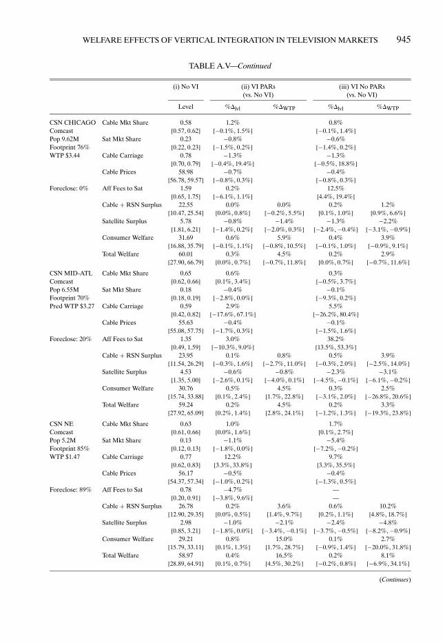
WELFARE EFFECTS OF VERTICAL INTEGRATION IN TELEVISION MARKETS 945
TABLE A.V—Continued
(i) No VI (ii) VI PARs (iii) VI No PARs(vs. No VI) (vs. No VI)
Level %�lvl %�WTP %�lvl %�WTP
CSN CHICAGO Cable Mkt Share 0.58 1.2% 0.8%Comcast [0�57�0�62] [−0�1%�1�5%] [−0�1%�1�4%]Pop 9.62M Sat Mkt Share 0.23 −0.8% −0.6%Footprint 76% [0�22�0�23] [−1�5%�0�2%] [−1�4%�0�2%]WTP $3.44 Cable Carriage 0.78 −1.3% −1.3%
[0�70�0�79] [−0�4%�19�4%] [−0�5%�18�8%]Cable Prices 58.98 −0.7% −0.4%
[56�78�59�57] [−0�8%�0�3%] [−0�8%�0�3%]Foreclose: 0% Aff Fees to Sat 1.59 0.2% 12.5%
[0�65�1�75] [−6�1%�1�1%] [4�4%�19�4%]Cable + RSN Surplus 22.55 0.0% 0.0% 0.2% 1.2%
[10�47�25�54] [0�0%�0�8%] [−0�2%�5�5%] [0�1%�1�0%] [0�9%�6�6%]Satellite Surplus 5.78 −0.8% −1.4% −1.3% −2.2%
[1�81�6�21] [−1�4%�0�2%] [−2�0%�0�3%] [−2�4%�−0�4%] [−3�1%�−0�9%]Consumer Welfare 31.69 0.6% 5.9% 0.4% 3.9%
[16�88�35�79] [−0�1%�1�1%] [−0�8%�10�5%] [−0�1%�1�0%] [−0�9%�9�1%]Total Welfare 60.01 0.3% 4.5% 0.2% 2.9%
[27�90�66�79] [0�0%�0�7%] [−0�7%�11�8%] [0�0%�0�7%] [−0�7%�11�6%]CSN MID-ATL Cable Mkt Share 0.65 0.6% 0.3%Comcast [0�62�0�66] [0�1%�3�4%] [−0�5%�3�7%]Pop 6.55M Sat Mkt Share 0.18 −0.4% −0.1%Footprint 70% [0�18�0�19] [−2�8%�0�0%] [−9�3%�0�2%]Pred WTP $3.27 Cable Carriage 0.59 2.9% 5.5%
[0�42�0�82] [−17�6%�67�1%] [−26�2%�80�4%]Cable Prices 55.63 −0.4% −0.1%
[55�08�57�75] [−1�7%�0�3%] [−1�5%�1�6%]Foreclose: 20% Aff Fees to Sat 1.35 3.0% 38.2%
[0�49�1�59] [−10�3%�9�0%] [13�5%�53�3%]Cable + RSN Surplus 23.95 0.1% 0.8% 0.5% 3.9%
[11�54�26�29] [−0�3%�1�6%] [−2�7%�11�0%] [−0�3%�2�0%] [−2�5%�14�0%]Satellite Surplus 4.53 −0.6% −0.8% −2.3% −3.1%
[1�35�5�00] [−2�6%�0�1%] [−4�0%�0�1%] [−4�5%�−0�1%] [−6�1%�−0�2%]Consumer Welfare 30.76 0.5% 4.5% 0.3% 2.5%
[15�74�33�88] [0�1%�2�4%] [1�7%�22�8%] [−3�1%�2�0%] [−26�8%�20�6%]Total Welfare 59.24 0.2% 4.5% 0.2% 3.3%
[27�92�65�09] [0�2%�1�4%] [2�8%�24�1%] [−1�2%�1�3%] [−19�3%�23�8%]CSN NE Cable Mkt Share 0.63 1.0% 1.7%Comcast [0�61�0�66] [0�0%�1�6%] [0�1%�2�7%]Pop 5.2M Sat Mkt Share 0.13 −1.1% −5.4%Footprint 85% [0�12�0�13] [−1�8%�0�0%] [−7�2%�−0�2%]WTP $1.47 Cable Carriage 0.77 12.2% 9.7%
[0�62�0�83] [3�3%�33�8%] [3�3%�35�5%]Cable Prices 56.17 −0.5% −0.4%
[54�37�57�34] [−1�0%�0�2%] [−1�3%�0�5%]Foreclose: 89% Aff Fees to Sat 0.78 −4.7% —
[0�20�0�91] [−3�8%�9�6%] —Cable + RSN Surplus 26.78 0.2% 3.6% 0.6% 10.2%
[12�90�29�35] [0�0%�0�5%] [1�4%�9�7%] [0�2%�1�1%] [4�8%�18�7%]Satellite Surplus 2.98 −1.0% −2.1% −2.4% −4.8%
[0�85�3�21] [−1�8%�0�0%] [−3�4%�−0�1%] [−3�7%�−0�5%] [−8�2%�−0�9%]Consumer Welfare 29.21 0.8% 15.0% 0.1% 2.7%
[15�79�33�11] [0�1%�1�3%] [1�7%�28�7%] [−0�9%�1�4%] [−20�0%�31�8%]Total Welfare 58.97 0.4% 16.5% 0.2% 8.1%
[28�89�64�91] [0�1%�0�7%] [4�5%�30�2%] [−0�2%�0�8%] [−6�9%�34�1%]
(Continues)

946 CRAWFORD, LEE, WHINSTON, AND YURUKOGLU
TABLE A.V—Continued
(i) No VI (ii) VI PARs (iii) VI No PARs(vs. No VI) (vs. No VI)
Level %�lvl %�WTP %�lvl %�WTP
MSG PLUS Cable Mkt Share 0.66 3.1% 3.1%Cablevision [0�65�0�70] [0�1%�5�1%] [0�1%�4�9%]Pop 9.46M Sat Mkt Share 0.19 −4.6% −4.6%Footprint 49% [0�17�0�19] [−7�5%�−0�4%] [−9�4%�−0�7%]WTP $1.66 Cable Carriage 0.42 54.6% 54.6%
[0�41�0�89] [−0�3%�85�8%] [−23�0%�85�8%]Cable Prices 59.59 −2.2% −2.2%
[57�46�61�09] [−4�0%�0�0%] [−3�8%�0�8%]Foreclose: 6% Aff Fees to Sat 0.75 0.9% 31.1%
[0�32�0�89] [−17�8%�17�0%] [2�6%�64�0%]Cable + RSN Surplus 32.81 0.6% 11.7% 0.7% 14.3%
[15�57�36�92] [−0�1%�0�9%] [−2�2%�17�0%] [−0�1%�1�3%] [−1�4%�24�0%]Satellite Surplus 4.39 −4.7% −12.3% −5.6% −14.8%
[1�32�4�71] [−7�5%�−0�3%] [−19�7%�−0�9%] [−7�8%�0�0%] [−21�6%�−0�1%]Consumer Welfare 35.59 3.2% 67.6% 3.1% 67.2%
[19�34�39�95] [0�4%�4�8%] [8�2%�110�9%] [−1�0%�4�5%] [−21�2%�108�9%]Total Welfare 72.78 1.5% 67.0% 1.5% 66.7%
[33�33�80�75] [0�2%�2�1%] [10�0%�96�8%] [−0�2%�2�0%] [−9�4%�95�8%]SNY Cable Mkt Share 0.63 3.8% 3.8%Comcast, TWC [0�62�0�67] [0�5%�6�1%] [0�5%�6�1%]Pop 11.7M Sat Mkt Share 0.18 −4.5% −4.5%Footprint 35% [0�17�0�18] [−8�2%�−0�7%] [−8�2%�−0�7%]WTP $2.51 Cable Carriage 0.79 1.9% 1.9%
[0�75�0�89] [−10�3%�8�3%] [−10�3%�7�7%]Cable Prices 59.80 −2.9% −2.9%
[56�97�61�32] [−4�5%�−0�3%] [−4�5%�−0�3%]a Foreclose: 0% Aff Fees to Sat 1.40 −4.0% −3.9%
[0�45�1�54] [−6�2%�6�3%] [−6�0%�6�3%]Cable + RSN Surplus 30.12 0.0% −0.6% 0.0% −0.6%
[14�34�33�64] [−0�6%�0�2%] [−9�6%�2�7%] [−0�6%�0�2%] [−9�6%�2�3%]Satellite Surplus 4.16 −4.3% −7.2% −4.3% −7.2%
[1�26�4�49] [−8�4%�−0�7%] [−13�8%�−1�1%] [−8�4%�−0�7%] [−13�8%�−1�1%]Consumer Welfare 33.69 3.3% 43.9% 3.3% 43.9%
[18�22�37�96] [0�4%�5�2%] [5�9%�72�8%] [0�4%�5�2%] [5�9%�72�8%]Total Welfare 67.96 1.3% 36.1% 1.3% 36.1%
[31�47�75�26] [0�2%�2�0%] [4�2%�58�3%] [0�2%�2�0%] [4�2%�58�3%]
aSimulated market outcomes across three integration scenarios. See Table IV for details.

WELFARE EFFECTS OF VERTICAL INTEGRATION IN TELEVISION MARKETS 947
TABLE A.VI
SIMULATED MARKET OUTCOMES FOR SATELLITE-OWNED RSNSa
(i) No VI (ii) VI PARs (iii) VI No PARs(vs. No VI) (vs. No VI)
Level %�lvl %�WTP %�lvl %�WTP
ROOT NW Cable Mkt Share 0.61 0.7% 0.6%DirecTV [0�58�0�62] [−0�4%�2�8%] [−0�6%�2�6%]Pop 4.15M Sat Mkt Share 0.23 −0.5% −0.4%WTP $1.79 [0�22�0�23] [−2�3%�0�4%] [−2�1%�1�1%]
Cable Carriage 0.78 0.0% 0.0%[0�52�1�00] [−13�4%�14�2%] [−31�3%�4�9%]
Cable Prices 52.90 −0.4% −0.4%[51�94�54�61] [−1�9%�0�3%] [−2�0%�0�4%]
Foreclose: 0% Aff Fees to Rivals 0.75 1.1% 6.4%[0�26�0�98] [−7�8%�3�1%] [−3�4%�11�3%]
Cable Surplus 21.94 0.0% −0.3% −0.2% −2.4%[9�99�25�20] [−0�2%�0�2%] [−2�1%�2�2%] [−0�6%�0�2%] [−5�8%�2�3%]
Satellite + RSN Surplus 6.69 −0.4% −1.4% 0.2% 0.9%[2�25�7�14] [−2�3%�1�1%] [−7�7%�3�3%] [−3�1%�1�0%] [−10�9%�3�0%]
Consumer Welfare 33.05 0.4% 7.6% 0.4% 6.7%[17�39�36�63] [−0�2%�1�7%] [−4�8%�31�3%] [−0�9%�1�6%] [−15�6%�28�9%]
Total Welfare 61.68 0.2% 5.9% 0.2% 5.2%[29�41�67�77] [−0�3%�0�8%] [−9�1%�27�5%] [−0�7%�0�7%] [−23�7%�24�9%]
ROOT PITT Cable Mkt Share 0.62 1.6% 1.1%DirecTV [0�60�0�63] [0�3%�2�4%] [−0�1%�2�1%]Pop 5.09M Sat Mkt Share 0.16 −1.9% −1.2%WTP $2.17 [0�16�0�16] [−2�2%�−0�2%] [−1�8%�0�7%]
Cable Carriage 0.62 0.0% −4.3%[0�51�0�69] [−22�1%�5�0%] [−29�4%�0�0%]
Cable Prices 55.64 −1.2% −1.0%[54�70�56�76] [−1�8%�−0�2%] [−1�9%�−0�1%]
Foreclose: 0% Aff Fees to Rivals 1.24 −0.1% 8.4%[0�53�1�51] [−2�2%�6�2%] [5�1%�19�7%]
Cable Surplus 23.54 0.0% −0.1% −0.3% −3.0%[10�87�25�69] [−0�4%�0�0%] [−4�2%�0�4%] [−0�7%�−0�1%] [−7�2%�−1�1%]
Satellite + RSN Surplus 5.04 −1.4% −3.3% −0.1% −0.1%[1�51�5�39] [−4�5%�0�0%] [−9�4%�0�1%] [−5�1%�1�0%] [−8�4%�2�3%]
Consumer Welfare 28.01 1.1% 14.5% 0.8% 10.7%[14�67�31�16] [0�2%�1�8%] [2�5%�25�4%] [−0�1%�1�6%] [−1�0%�22�2%]
Total Welfare 56.59 0.4% 11.1% 0.3% 7.6%[27�15�61�63] [−0�2%�0�6%] [−4�5%�16�5%] [−0�4%�0�5%] [−9�8%�13�2%]
ROOT ROCKY MTN Cable Mkt Share 0.50 0.0% 1.0%DirecTV [0�44�0�53] [−5�1%�0�0%] [−7�0%�2�9%]Pop 4.19M Sat Mkt Share 0.30 0.0% −0.3%WTP $1.79 [0�29�0�33] [0�0%�4�5%] [−1�0%�5�6%]
Cable Carriage 0.59 0.0% −17.3%[0�48�0�84] [−27�5%�0�0%] [−37�0%�0�0%]
Cable Prices 55.84 0.0% −0.7%[54�03�59�28] [−0�2%�2�4%] [−1�5%�3�1%]
a Foreclose: 0% Aff Fees to Rivals 0.96 0.3% 7.9%[0�26�1�29] [−0�5%�15�5%] [4�6%�28�7%]
Cable Surplus 13.89 0.0% −0.1% −0.4% −3.1%[6�45�15�15] [−0�8%�0�0%] [−5�6%�0�2%] [−1�4%�−0�2%] [−10�2%�−0�7%]
Satellite + RSN Surplus 8.90 0.0% 0.2% −0.9% −4.3%[3�10�9�44] [−1�2%�3�6%] [−4�0%�16�9%] [−2�7%�4�8%] [−13�9%�22�8%]
Consumer Welfare 32.59 0.0% −0.4% 0.3% 4.9%[16�28�35�90] [−2�5%�0�0%] [−55�1%�0�3%] [−2�7%�0�9%] [−63�3%�19�7%]
Total Welfare 55.38 0.0% −0.3% −0.1% −2.4%[25�12�60�28] [−1�1%�0�0%] [−47�3%�0�0%] [−1�3%�0�0%] [−50�2%�0�1%]
aSimulated market outcomes across three integration scenarios. “Satellite + RSN Surplus” includes profits for both DirecTV andDish. See Table IV for details.

948 CRAWFORD, LEE, WHINSTON, AND YURUKOGLU
TABLE A.VII
SIMULATED MARKET OUTCOMES FOR NON-INTEGRATED RSNSa
(i) No VI (ii) VI PARs (iii) VI No PARs(vs. No VI) (vs. No VI)
Level %�lvl %�WTP %�lvl %�WTP
ALTITUDE Cable Mkt Share 0.54 0.2% 0.1%*Comcast [0�48�0�57] [−0�9%�6�1%] [−1�0%�5�2%]Pop 7.12M Sat Mkt Share 0.28 −0.1% −0.1%Footprint 74% [0�26�0�30] [−5�9%�0�3%] [−5�2%�0�4%]WTP $3.22 Cable Carriage 0.48 0.0% 0.0%
[0�23�0�60] [0�0%�213�0%] [0�0%�213�0%]Cable Prices 56.41 −0.1% −0.1%
[54�26�59�69] [−2�8%�1�2%] [−2�6%�1�2%]Foreclose: 1% Aff Fees to Sat 1.20 5.0% 33.8%
[0�39�1�48] [−21�2%�10�8%] [2�0%�52�8%]Cable + RSN Surplus 16.97 0.1% 0.6% 0.7% 3.5%
[8�43�18�54] [0�1%�2�4%] [0�4%�13�2%] [0�5%�2�9%] [2�7%�16�5%]Satellite Surplus 6.97 −0.4% −0.8% −1.7% −3.6%
[2�12�7�54] [−5�8%�0�2%] [−10�9%�0�4%] [−5�4%�−0�6%] [−12�1%�−0�8%]Consumer Welfare 32.60 0.1% 0.8% 0.0% 0.4%
[16�47�36�56] [−0�2%�3�0%] [−2�6%�28�9%] [−1�0%�2�3%] [−10�0%�26�2%]Total Welfare 56.54 0.0% 0.6% 0.0% 0.3%
[26�28�62�37] [−0�1%�1�4%] [−1�2%�23�3%] [−0�4%�1�1%] [−6�3%�20�7%]FS DETROIT Cable Mkt Share 0.56 3.1% 3.0%*Comcast [0�54�0�58] [0�3%�6�4%] [0�2%�6�3%]Pop 4.84M Sat Mkt Share 0.17 −3.7% −3.6%Footprint 82% [0�17�0�18] [−7�1%�−0�4%] [−11�8%�−0�3%]WTP $4.38 Cable Carriage 0.76 27.6% 27.6%
[0�55�0�87] [6�7%�77�4%] [6�7%�77�4%]Cable Prices 50.34 −1.0% −1.0%
[49�71�51�44] [−3�0%�0�1%] [−2�8%�0�5%]Foreclose: 7% Aff Fees to Sat 2.10 −11.4% 12.7%
[0�76�2�69] [−30�7%�2�4%] [−14�9%�33�3%]Cable + RSN Surplus 20.37 1.2% 5.6% 1.6% 7.5%
[9�70�22�30] [0�3%�2�5%] [1�8%�11�5%] [0�7%�3�1%] [3�7%�13�0%]Satellite Surplus 4.38 −2.8% −2.8% −4.6% −4.6%
[1�33�4�74] [−4�9%�−0�3%] [−4�8%�−0�4%] [−6�8%�−1�4%] [−6�3%�−1�8%]Consumer Welfare 26.64 2.4% 14.4% 2.3% 13.9%
[13�84�29�68] [0�2%�5�2%] [1�4%�30�8%] [−1�5%�5�0%] [−9�2%�30�2%]Total Welfare 51.38 1.5% 17.2% 1.4% 16.8%
[24�53�56�31] [0�2%�3�3%] [3�7%�38�5%] [−0�2%�3�2%] [−2�7%�36�6%]FS FLORIDA Cable Mkt Share 0.60 0.8% 0.7%*Comcast [0�59�0�61] [0�1%�3�4%] [−0�1%�3�1%]Pop 6.20M Sat Mkt Share 0.23 −0.8% −0.7%Footprint 67% [0�22�0�23] [−3�7%�−0�1%] [−9�6%�0�0%]WTP $2.59 Cable Carriage 0.90 2.2% 2.2%
[0�53�0�94] [0�5%�68�6%] [0�0%�68�6%]Cable Prices 54.19 −0.4% −0.3%
[53�95�54�93] [−1�4%�0�2%] [−1�1%�1�0%]a Foreclose: 9% Aff Fees to Sat 1.47 −0.7% 25.8%
[0�64�1�71] [−14�1%�5�5%] [3�3%�40�1%]Cable + RSN Surplus 19.84 0.1% 0.9% 0.6% 4.4%
[8�90�21�98] [0�1%�1�6%] [0�5%�13�0%] [0�3%�2�1%] [3�5%�16�5%]Satellite Surplus 6.08 −0.8% −1.9% −2.2% −5.2%
[1�79�6�69] [−3�3%�−0�2%] [−9�7%�−0�5%] [−4�5%�−0�6%] [−12�8%�−1�3%]Consumer Welfare 31.20 0.5% 5.5% 0.4% 4.6%
[15�35�34�16] [0�1%�2�4%] [1�2%�35�4%] [−2�7%�2�2%] [−33�2%�32�5%]Total Welfare 57.11 0.2% 4.5% 0.2% 3.9%
[24�93�62�59] [0�1%�1�3%] [1�3%�37�2%] [−1�2%�1�3%] [−25�1%�35�6%]
(Continues)

WELFARE EFFECTS OF VERTICAL INTEGRATION IN TELEVISION MARKETS 949
TABLE A.VII—Continued
(i) No VI (ii) VI PARs (iii) VI No PARs(vs. No VI) (vs. No VI)
Level %�lvl %�WTP %�lvl %�WTP
FS MIDWEST Cable Mkt Share 0.60 1.8% 1.7%*Comcast [0�59�0�62] [0�1%�2�1%] [0�1%�2�1%]Pop 10.40M Sat Mkt Share 0.21 −1.2% −1.2%Footprint 26% [0�21�0�21] [−1�5%�0�0%] [−1�5%�0�1%]WTP $2.44 Cable Carriage 0.43 29.5% 29.5%
[0�26�0�55] [3�3%�51�4%] [−13�9%�50�4%]Cable Prices 52.15 −0.8% −0.7%
[51�19�52�45] [−1�0%�0�1%] [−1�0%�0�1%]Foreclose: 0% Aff Fees to Sat 1.18 −1.5% 17.1%
[0�55�1�31] [−6�5%�3�1%] [10�5%�31�9%]Cable + RSN Surplus 19.92 0.3% 2.8% 0.6% 4.7%
[9�44�21�77] [0�0%�0�6%] [0�0%�4�8%] [−0�1%�0�7%] [−0�9%�6�8%]Satellite Surplus 5.26 −1.2% −2.6% −2.0% −4.4%
[1�69�5�66] [−1�4%�0�0%] [−2�7%�−0�2%] [−2�5%�−0�7%] [−4�7%�−1�9%]Consumer Welfare 29.92 1.3% 15.8% 1.3% 15.6%
[15�57�33�40] [0�1%�1�4%] [1�2%�16�7%] [0�0%�1�4%] [0�1%�16�6%]Total Welfare 55.10 0.7% 16.0% 0.7% 15.9%
[26�21�60�16] [0�1%�0�8%] [1�3%�16�6%] [−0�1%�0�8%] [−2�5%�16�5%]FS NORTH Cable Mkt Share 0.61 0.1% 0.1%*Charter [0�59�0�64] [0�0%�0�7%] [0�0%�0�7%]Pop 5.77M Sat Mkt Share 0.15 −0.2% −0.2%Footprint 12% [0�14�0�16] [−1�4%�0�0%] [−1�4%�0�0%]WTP $4.50 Cable Carriage 0.87 0.0% 0.0%
[0�62�0�90] [0�0%�7�4%] [0�0%�7�1%]Cable Prices 52.04 −0.1% −0.1%
[50�73�53�33] [−0�3%�0�1%] [−0�3%�0�1%]Foreclose: 0% Aff Fees to Sat 2.42 0.5% 7.7%
[0�89�3�09] [−7�1%�1�7%] [−0�4%�12�6%]Cable + RSN Surplus 23.02 0.0% 0.1% 0.1% 0.6%
[10�75�25�23] [0�0%�0�4%] [0�0%�1�8%] [0�1%�0�4%] [0�6%�2�0%]Satellite Surplus 3.71 −0.2% −0.2% −0.9% −0.8%
[1�22�4�00] [−1�1%�0�0%] [−0�8%�0�0%] [−2�0%�−0�5%] [−1�4%�−0�6%]Consumer Welfare 27.70 0.1% 0.6% 0.1% 0.6%
[14�35�31�04] [0�0%�0�6%] [0�0%�3�7%] [0�0%�0�6%] [−0�1%�3�6%]Total Welfare 54.43 0.0% 0.5% 0.0% 0.5%
[25�87�59�69] [0�0%�0�3%] [0�0%�4�5%] [0�0%�0�3%] [−0�1%�3�9%]FS OHIO Cable Mkt Share 0.60 2.0% 2.0%*TWC [0�60�0�62] [0�1%�2�4%] [0�1%�2�4%]Pop 8.16M Sat Mkt Share 0.18 −1.7% −1.7%Footprint 51% [0�18�0�18] [−2�5%�−0�1%] [−2�6%�0�0%]WTP $3.70 Cable Carriage 0.72 5.3% 5.3%
[0�41�0�78] [0�0%�46�0%] [0�0%�46�0%]Cable Prices 52.43 −1.2% −1.2%
[51�32�52�52] [−1�3%�0�2%] [−1�2%�0�3%]a Foreclose: 1% Aff Fees to Sat 1.72 2.4% 20.1%
[0�75�1�94] [−7�1%�8�8%] [5�4%�32�3%]Cable + RSN Surplus 22.39 0.3% 1.6% 0.5% 3.0%
[10�30�25�14] [0�0%�1�4%] [0�3%�9�1%] [0�3%�1�7%] [1�7%�10�8%]Satellite Surplus 4.47 −1.9% −2.2% −3.1% −3.7%
[1�39�4�76] [−2�3%�−0�2%] [−2�7%�−0�2%] [−4�0%�−0�6%] [−3�9%�−0�8%]Consumer Welfare 28.65 1.4% 10.7% 1.4% 10.5%
[15�23�32�22] [0�1%�2�2%] [0�7%�17�3%] [0�0%�2�1%] [0�3%�16�0%]Total Welfare 55.51 0.7% 10.0% 0.7% 9.9%
[26�41�61�52] [0�1%�1�4%] [0�8%�23�9%] [0�0%�1�4%] [0�7%�22�4%]
(Continues)
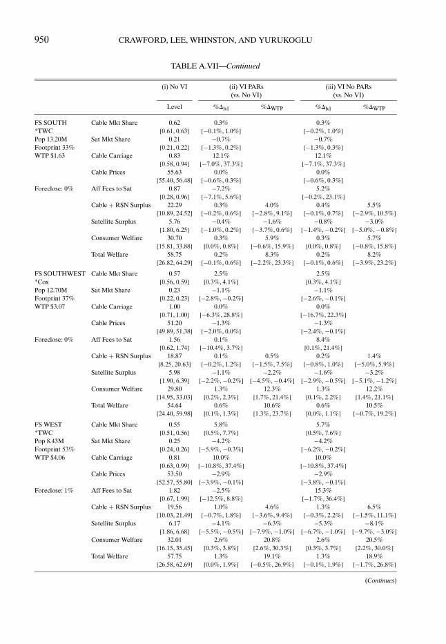
950 CRAWFORD, LEE, WHINSTON, AND YURUKOGLU
TABLE A.VII—Continued
(i) No VI (ii) VI PARs (iii) VI No PARs(vs. No VI) (vs. No VI)
Level %�lvl %�WTP %�lvl %�WTP
FS SOUTH Cable Mkt Share 0.62 0.3% 0.3%*TWC [0�61�0�63] [−0�1%�1�0%] [−0�2%�1�0%]Pop 13.20M Sat Mkt Share 0.21 −0.7% −0.7%Footprint 33% [0�21�0�22] [−1�3%�0�2%] [−1�3%�0�3%]WTP $1.63 Cable Carriage 0.83 12.1% 12.1%
[0�58�0�94] [−7�0%�37�3%] [−7�1%�37�3%]Cable Prices 55.63 0.0% 0.0%
[55�40�56�48] [−0�6%�0�3%] [−0�6%�0�3%]Foreclose: 0% Aff Fees to Sat 0.87 −7.2% 5.2%
[0�28�0�96] [−7�1%�5�6%] [−0�2%�23�1%]Cable + RSN Surplus 22.29 0.3% 4.0% 0.4% 5.5%
[10�89�24�52] [−0�2%�0�6%] [−2�8%�9�1%] [−0�1%�0�7%] [−2�9%�10�5%]Satellite Surplus 5.76 −0.4% −1.6% −0.8% −3.0%
[1�80�6�25] [−1�0%�0�2%] [−3�7%�0�6%] [−1�4%�−0�2%] [−5�0%�−0�8%]Consumer Welfare 30.70 0.3% 5.9% 0.3% 5.7%
[15�81�33�88] [0�0%�0�8%] [−0�6%�15�9%] [0�0%�0�8%] [−0�8%�15�8%]Total Welfare 58.75 0.2% 8.3% 0.2% 8.2%
[26�82�64�29] [−0�1%�0�6%] [−2�2%�23�3%] [−0�1%�0�6%] [−3�9%�23�2%]FS SOUTHWEST Cable Mkt Share 0.57 2.5% 2.5%*Cox [0�56�0�59] [0�3%�4�1%] [0�3%�4�1%]Pop 12.70M Sat Mkt Share 0.23 −1.1% −1.1%Footprint 37% [0�22�0�23] [−2�8%�−0�2%] [−2�6%�−0�1%]WTP $3.07 Cable Carriage 1.00 0.0% 0.0%
[0�71�1�00] [−6�3%�28�8%] [−16�7%�22�3%]Cable Prices 51.20 −1.3% −1.3%
[49�89�51�38] [−2�0%�0�0%] [−2�4%�−0�1%]Foreclose: 0% Aff Fees to Sat 1.56 0.1% 8.4%
[0�62�1�74] [−10�4%�3�7%] [0�1%�21�4%]Cable + RSN Surplus 18.87 0.1% 0.5% 0.2% 1.4%
[8�25�20�63] [−0�2%�1�2%] [−1�5%�7�5%] [−0�8%�1�0%] [−5�0%�5�9%]Satellite Surplus 5.98 −1.1% −2.2% −1.6% −3.2%
[1�90�6�39] [−2�2%�−0�2%] [−4�5%�−0�4%] [−2�9%�−0�5%] [−5�1%�−1�2%]Consumer Welfare 29.80 1.3% 12.3% 1.3% 12.2%
[14�95�33�03] [0�2%�2�3%] [1�7%�21�4%] [0�1%�2�2%] [1�4%�21�1%]Total Welfare 54.64 0.6% 10.6% 0.6% 10.5%
[24�40�59�98] [0�1%�1�3%] [1�3%�23�7%] [0�0%�1�1%] [−0�7%�19�2%]FS WEST Cable Mkt Share 0.55 5.8% 5.7%*TWC [0�51�0�56] [0�5%�7�7%] [0�5%�7�6%]Pop 8.43M Sat Mkt Share 0.25 −4.2% −4.2%Footprint 53% [0�24�0�26] [−5�9%�−0�3%] [−6�2%�−0�2%]WTP $4.06 Cable Carriage 0.81 10.0% 10.0%
[0�63�0�99] [−10�8%�37�4%] [−10�8%�37�4%]Cable Prices 53.50 −2.9% −2.9%
[52�57�55�80] [−3�9%�−0�1%] [−3�8%�−0�1%]Foreclose: 1% Aff Fees to Sat 1.82 −2.5% 15.3%
[0�67�1�99] [−12�5%�8�8%] [−1�7%�36�4%]Cable + RSN Surplus 19.56 1.0% 4.6% 1.3% 6.5%
[10�03�21�49] [−0�7%�1�8%] [−3�6%�9�4%] [−0�3%�2�2%] [−1�5%�11�1%]Satellite Surplus 6.17 −4.1% −6.3% −5.3% −8.1%
[1�86�6�68] [−5�5%�−0�5%] [−7�9%�−1�0%] [−6�7%�−1�0%] [−9�7%�−3�0%]Consumer Welfare 32.01 2.6% 20.8% 2.6% 20.5%
[16�15�35�45] [0�3%�3�8%] [2�6%�30�3%] [0�3%�3�7%] [2�2%�30�0%]Total Welfare 57.75 1.3% 19.1% 1.3% 18.9%
[26�58�62�69] [0�0%�1�9%] [−0�5%�26�9%] [−0�1%�1�9%] [−1�7%�26�8%]
(Continues)

WELFARE EFFECTS OF VERTICAL INTEGRATION IN TELEVISION MARKETS 951
TABLE A.VII—Continued
(i) No VI (ii) VI PARs (iii) VI No PARs(vs. No VI) (vs. No VI)
Level %�lvl %�WTP %�lvl %�WTP
MASN Cable Mkt Share 0.64 4.5% 4.4%*Comcast [0�61�0�66] [1�0%�5�6%] [0�9%�5�5%]Pop 8.25M Sat Mkt Share 0.18 −4.1% −3.9%Footprint 52% [0�17�0�18] [−7�1%�−1�0%] [−10�7%�−1�0%]WTP $2.21 Cable Carriage 0.51 10.2% 6.1%
[0�41�0�71] [2�6%�39�0%] [2�2%�39�0%]Cable Prices 56.71 −2.5% −2.6%
[55�59�58�38] [−2�9%�−0�1%] [−2�8%�−0�1%]Foreclose: 3% Aff Fees to Sat 1.47 0.2% 27.2%
[0�53�1�70] [−7�4%�6�8%] [13�9%�38�5%]Cable + RSN Surplus 23.52 0.1% 1.0% 0.3% 3.3%
[11�47�26�15] [−0�1%�0�9%] [−1�6%�8�5%] [0�1%�1�5%] [1�3%�16�5%]Satellite Surplus 4.44 −4.2% −8.4% −5.7% −11.4%
[1�34�4�87] [−6�6%�−0�9%] [−14�0%�−2�6%] [−7�5%�−1�5%] [−16�8%�−4�6%]Consumer Welfare 29.80 3.4% 45.3% 3.3% 44.4%
[15�53�32�88] [0�8%�4�2%] [11�3%�65�2%] [−0�7%�4�2%] [−9�9%�64�3%]Total Welfare 57.76 1.5% 37.9% 1.4% 36.3%
[27�68�63�28] [0�4%�1�9%] [12�7%�51�3%] [−0�1%�1�9%] [−1�8%�51�2%]PRIME TICKET Cable Mkt Share 0.55 3.2% 3.2%*TWC [0�51�0�56] [0�4%�7�1%] [0�5%�6�8%]Pop 8.32M Sat Mkt Share 0.25 −2.2% −2.2%Footprint 53% [0�24�0�26] [−4�7%�−0�3%] [−4�7%�−0�3%]WTP $3.11 Cable Carriage 0.79 8.3% 8.3%
[0�60�0�87] [−1�0%�23�8%] [−1�0%�23�8%]Cable Prices 53.29 −1.7% −1.7%
[52�73�55�97] [−3�6%�−0�1%] [−3�3%�−0�1%]Foreclose: 1% Aff Fees to Sat 1.48 0.2% 18.3%
[0�59�1�70] [−8�3%�6�1%] [3�5%�34�2%]Cable + RSN Surplus 19.19 0.5% 3.0% 0.8% 5.0%
[9�68�21�21] [0�0%�1�0%] [−0�1%�6�5%] [0�3%�1�5%] [1�8%�9�7%]Satellite Surplus 6.09 −2.2% −4.3% −3.2% −6.2%
[1�86�6�69] [−4�6%�−0�4%] [−9�0%�−1�0%] [−5�7%�−0�9%] [−10�5%�−2�7%]Consumer Welfare 32.33 1.5% 15.5% 1.5% 15.2%
[16�15�35�63] [0�3%�3�5%] [3�4%�34�9%] [0�3%�3�4%] [3�1%�34�6%]Total Welfare 57.61 0.8% 14.2% 0.8% 14.1%
[26�19�62�28] [0�2%�1�7%] [3�9%�29�1%] [0�1%�1�6%] [3�5%�28�7%]SUN SPORTS Cable Mkt Share 0.60 1.4% 1.3%*TWC [0�59�0�61] [0�1%�2�2%] [0�1%�2�2%]Pop 3.41M Sat Mkt Share 0.18 −1.2% −1.2%Footprint 65% [0�17�0�18] [−1�8%�0�0%] [−1�8%�0�1%]WTP $1.65 Cable Carriage 0.97 0.0% 0.0%
[0�84�0�97] [−2�0%�7�4%] [−2�0%�7�4%]Cable Prices 55.39 −0.7% −0.7%
[54�84�56�06] [−1�1%�0�0%] [−1�1%�0�0%]a Foreclose: 0% Aff Fees to Sat 0.62 −0.2% 17.1%
[0�29�0�81] [−5�3%�6�1%] [8�8%�33�3%]Cable + RSN Surplus 18.85 0.0% 0.3% 0.1% 1.5%
[8�69�21�04] [−0�1%�0�5%] [−1�3%�5�7%] [0�0%�0�5%] [−0�2%�7�2%]Satellite Surplus 4.61 −1.3% −3.5% −1.7% −4.7%
[1�36�4�94] [−1�7%�−0�1%] [−4�8%�−0�2%] [−2�3%�−0�3%] [−6�2%�−1�1%]Consumer Welfare 27.02 1.0% 16.9% 1.0% 16.7%
[13�49�29�81] [0�1%�1�7%] [1�5%�26�7%] [0�0%�1�7%] [0�5%�26�7%]Total Welfare 50.48 0.4% 13.7% 0.4% 13.5%
[22�93�55�42] [0�0%�0�9%] [1�2%�25�2%] [0�0%�0�9%] [1�1%�25�1%]
aSimulated market outcomes across three integration scenarios. See Table IV for details.

952C
RA
WF
OR
D,L
EE
,WH
INST
ON
,AN
DY
UR
UK
OG
LU
TABLE A.VIII
AVERAGE SIMULATED MARKET OUTCOMES ACROSS ALL RSNS (SATELLITE ADJUSTS PRICES)a
(i) No VI (ii) VI PARs (iii) VI No PARs
(vs. No VI) (vs. No VI) (vs. VI PARs)
Level %�lvl %�WTP %�lvl %�WTP %�lvl %�WTP
All RSNsCable Mkt Share 0.61 1.5% 1.5% 0.0%
[0�61�0�62] [0�2%�2�1%] [0�4%�2�1%] [−0�2%�0�2%]Sat Mkt Share 0.19 0.0% −0.5% −0.5%
[0�18�0�20] [−1�3%�1�1%] [−2�0%�0�8%] [−1�2%�0�3%]Cable Carriage 0.75 5.8% 5.4% −0.4%
[0�69�0�80] [4�0%�15�9%] [3�4%�15�7%] [−2�4%�1�1%]Cable Prices 55.06 −1.1% −1.0% 0.1%
[54�25�55�98] [−1�5%�−0�1%] [−1�4%�0�0%] [0�0%�0�4%]Sat Prices 57.75 −0.8% −1.0% −0.1%
[56�34�61�30] [−1�5%�−0�1%] [−1�8%�0�0%] [−0�5%�0�3%]Aff Fees to Rivals 1.48 −1.8% 16.5% 18.2%
[0�46�1�76] [−5�2%�1�7%] [1�9%�43�0%] [8�0%�50�3%]Cable + RSN Surplus 23.10 0.2% 1.9% 0.5% 4.0% 0.3% 2.1%
[10�40�25�27] [0�2%�0�5%] [0�9%�7�5%] [0�3%�0�7%] [1�7%�14�2%] [0�1%�0�4%] [0�4%�5�5%]Satellite Surplus 5.06 −1.9% −3.7% −2.8% −5.4% −1.0% −1.7%
[1�56�5�44] [−2�8%�−0�5%] [−9�4%�−0�3%] [−3�6%�−1�2%] [−12�1%�−0�9%] [−1�3%�−0�5%] [−3�5%�−0�4%]Consumer Welfare 31.02 1.4% 17.4% 1.2% 15.6% −0.2% −1.8%
[13�10�34�10] [0�3%�1�8%] [2�4%�33�4%] [0�0%�1�6%] [−0�2%�29�5%] [−0�7%�−0�1%] [−10�0%�−0�2%]Total Welfare 59.17 0.7% 15.7% 0.6% 14.2% −0.1% −1.5%
[24�85�64�45] [0�2%�0�8%] [2�6%�32�2%] [0�1%�0�8%] [1�4%�29�2%] [−0�3%�0�0%] [−8�7%�−0�3%]# Foreclosed: 4/26 [1�9]aAverage simulated market outcomes for all RSNs, weighted by the number of households in each RSN’s relevant DMAs, where satellite prices are allowed to adjust. See Table V and Ap-
pendix S.B.4 of the Supplemental Material for details.

WELFARE EFFECTS OF VERTICAL INTEGRATION IN TELEVISION MARKETS 953
REFERENCES
ACKERBERG, D. A. (2009): “A New Use of Importance Sampling to Reduce Computational Burden in Simu-lation Estimation,” Quantitative Marketing and Economics, 7 (4), 343–376. [915]
ASKER, J. (2016): “Diagnosing Foreclosure Due to Exclusive Dealing,” Journal of Industrial Economics, 64 (3),375–410. [895]
ATALAY, E., A. HORTAÇSU, M. J. LI, AND C. SYVERSON (2017): “How Wide Is the Firm Border?” NBERWorking Paper 23777. [895]
ATALAY, E., A. HORTAÇSU, AND C. SYVERSON (2014): “Vertical Integration and Input Flows,” American Eco-nomic Review, 104 (4), 1120–1148. [895]
BERRY, S., J. LEVINSOHN, AND A. PAKES (1995): “Automobile Prices in Market Equilibrium,” Econometrica,63 (4), 841–890. [915]
BOLTON, P., AND M. D. WHINSTON (1991): “The ‘Foreclosure’ Effects of Vertical Mergers,” Journal of Institu-tional and Theoretical Economics, 147, 207–226. [894,938]
BRESNAHAN, T., AND J. LEVIN (2013): “Vertical Integration and Market Structure,” in Handbook of Orga-nizational Economics, ed. by R. Gibbons and J. Roberts. Princeton, NJ: Princeton University Press. [891,
895]CAVES, K. W., C. C. HOLT, AND H. J. SINGER (2013): “Vertical Integration in Multichannel Television Markets:
A Study of Regional Sports Networks,” Review of Network Economics, 12 (1), 61–92. [894]CHEN, D., AND D. WATERMAN (2007): “Vertical Ownership, Program Network Carriage, and Tier Positioning
in Cable Television: An Empirical Study,” Review of Industrial Organization, 30 (3), 227–251. [894]CHEN, Y. (2001): “On Vertical Mergers and Their Competitive Effects,” RAND Journal of Economics, 32 (4),
667–685. [910,929,936]CHIPTY, T. (2001): “Vertical Integration, Market Foreclosure, and Consumer Welfare in the Cable Television
Industry,” American Economic Review, 91 (3), 428–453. [894]CILIBERTO, F. (2006): “Does Organizational Form Affect Investment Decisions?” Journal of Industrial Eco-
nomics, 54 (1), 63–93. [895]COLLARD-WEXLER, A., G. GOWRISANKARAN, AND R. S. LEE (2018): “‘Nash-in-Nash’ Bargaining: A Micro-
foundation for Applied Work,” Journal of Political Economy (forthcoming). [910,911,921]CONLON, C. T., AND J. H. MORTIMER (2016): “Efficiency and Foreclosure Effects of Vertical Rebates: Empir-
ical Evidence,” NBER Working Paper 19709. [895]CRAWFORD, G. S, R. S LEE M. D WHINSTON, A. YURUKOGLU (2018): “Supplement to ‘The Welfare Effects
of Vertical Integration in Multichannel Television Markets’,” Econometrica Supplemental Material, 88, http://dx.doi.org/ECTA14031. [905,909]
CRAWFORD, G. S., AND A. YURUKOGLU (2012): “The Welfare Effects of Bundling in Multichannel TelevisionMarkets,” American Economic Review, 102 (2), 643–685. [892,896,901-903,910,918]
DRAGANSKA, M., D. KLAPPER, AND S. B. VILLAS-BOAS (2010): “A Larger Slice or a Larger Pie? An EmpiricalInvestigation of Bargaining Power in the Distribution Channel,” Marketing Science, 29 (1), 57–74. [910,911]
DUBIN, J. A., AND D. L. MCFADDEN (1984): “An Econometric Analysis of Residential Electric ApplianceHoldings and Consumption,” Econometrica, 52 (2), 345–362. [902]
FCC (2012): “Report and Order in MB Docket Nos. 12-68, 07-18, 05-192; Further Notice of Proposed Rule-making in MB Docket No. 12-68; Order on Reconsideration in MB Docket No. 07-29,” Technical ReportFCC 12-123, released October 5, 2012. [898]
(2013): “Fifteenth Report: Annual Assessment of the Status of Competition in the Market for theDelivery of Video Programming,” Technical Report FCC 13-99, released July 22, 2013. [895]
GOOLSBEE, A., AND A. PETRIN (2004): “Consumer Gains From Direct Broadcast Satellites and the Competi-tion With Cable TV,” Econometrica, 72 (2), 351–381. [924]
GOURIÉROUX, C., AND A. MONFORT (1996): Simulation-Based Econometric Methods. Oxford: Oxford Univer-sity Press. [916]
GOWRISANKARAN, G., A. NEVO, AND R. TOWN (2015): “Mergers When Prices Are Negotiated: EvidenceFrom the Hospital Industry,” American Economic Review, 105 (1), 172–203. [910]
GRENNAN, M. (2013): “Price Discrimination and Bargaining: Empirical Evidence From Medical Devices,”American Economic Review, 103 (1), 147–177. [910]
GROSSMAN, S., AND O. HART (1986): “The Costs and Benefits of Ownership: A Theory of Vertical and LateralIntegration,” Journal of Political Economy, 94, 691–796. [891,938]
HANEMANN, W. M. (1984): “Discrete/Continuous Models of Consumer Demand,” Econometrica, 52 (3), 541–561. [902]
HART, O. (1995): Firms, Contracts, and Financial Structure. New York: Oxford University Press. [894,938]HART, O., AND J. TIROLE (1990): “Vertical Integration and Market Foreclosure,” Brookings Papers on Eco-
nomic Activity: Microeconomics, 1990, 205–286. [891]

954 CRAWFORD, LEE, WHINSTON, AND YURUKOGLU
HASTINGS, J. S. (2004): “Vertical Relationships and Competition in Retail Gasoline Markets: Empirical Evi-dence From Contract Changes in Southern California,” American Economic Review, 94, 317–328. [895]
HASTINGS, J. S., AND R. J. GILBERT (2005): “Market Power, Vertical Integration and the Wholesale Price ofGasoline,” Journal of Industrial Economics, 53 (4), 469–492. [895]
HO, K., AND R. S. LEE (2017): “Insurer Competition in Health Care Markets,” Econometrica, 85 (2), 379–417.[895,910,911]
HORN, H., AND A. WOLINSKY (1988): “Bilateral Monopoly and Incentives for Merger,” RAND Journal ofEconomics, 19, 408–419. [910]
HORTAÇSU, A., AND C. SYVERSON (2007): “Cementing Relationships: Vertical Integration, Foreclosure, Pro-ductivity and Prices,” Journal of Political Economy, 115 (2), 250–301. [895]
HOUDE, J.-F. (2012): “Spatial Differentiation and Vertical Mergers in Retail Markets for Gasoline,” AmericanEconomic Review, 102 (5), 2147–2182. [895]
KRATTENMAKER, T. G., AND S. C. SALOP (1986): “Anticompetitive Exclusion: Raising Rivals’ Costs to AchievePower Over Price,” The Yale Law Journal, 2, 209–293. [891,908]
LEE, R. S. (2013): “Vertical Integration and Exclusivity in Platform and Two-Sided Markets,” American Eco-nomic Review, 103 (7), 2960–3000. [895]
MICHEL, C. (2016): “Identification and Estimation of Intra-Firm and Industry Competition via OwnershipChange,” Unpublished manuscript. [895]
MORTIMER, J. H. (2008): “Vertical Contracts in the Video Rental Industry,” Review of Economic Studies, 75,165–199. [895]
NOCKE, V., AND L. WHITE (2007): “Do Vertical Mergers Facilitate Upstream Collusion,” American EconomicReview, 97 (4), 1321–1339. [911]
ORDOVER, J., G. SALONER, AND S. SALOP (1990): “Equilibrium Vertical Foreclosure,” American EconomicReview, 80, 127–142. [891]
PERRY, M. K. (1990): “Vertical Integration: Determinants and Effects,” in Handbook of Industrial Organization,Vol. 1, ed. by R. Schmalensee and R. Willig. Amsterdam: North-Holland. [891]
REY, P., AND J. TIROLE (2007): “A Primer on Foreclosure,” in Handbook of Industrial Organization, Vol. 3, ed.by M. Armstrong and R. Porter. Amsterdam: North-Holland. [891]
RIORDAN, M. H. (2008): “Competitive Effects of Vertical Integration,” in Handbook of Antitrust Economics,ed. by P. Buccirossi. Cambridge, MA: MIT Press. [891]
ROGERSON, W. P. (2014): “Vertical Mergers in the Video Programming and Distribution Industry: The Case ofComcast-NBCU,” in The Antitrust Revolution (Sixth Ed.), ed. by J. E. Kwoka Jr. and L. J. White. New York:Oxford University Press. [911]
SALOP, S. C., AND D. T. SCHEFFMAN (1983): “Raising Rivals’ Costs,” American Economic Review, 73 (2), 267–271. [891,908,922]
SHEPARD, A. (1993): “Contractual Form, Retail Price, and Asset Characteristics in Gasoline Retailing,” RANDJournal of Economics, 24 (1), 58–77. [895]
SPENGLER, J. J. (1950): “Vertical Integration and Antitrust Policy,” Journal of Political Economy, 58 (4), 347–352. [891]
SUZUKI, A. (2009): “Market Foreclosure and Vertical Merger: A Case Study of the Vertical Merger BetweenTurner Broadcasting and Time Warner,” International Journal of Industrial Organization, 27 (4), 523–543.[894]
VILLAS-BOAS, S. B. (2007): “Vertical Relationships Between Manufacturers and Retailers: Inference WithLimited Data,” Review of Economic Studies, 74 (2), 625–652. [895]
WATERMAN, D., AND A. A. WEISS (1996): “The Effects of Vertical Integration Between Cable TelevisionSystems and Pay Cable Networks,” Journal of Econometrics, 72 (1–2), 357–395. [894,938]
WILLAMSON, O. (1985): The Economic Institutions of Capitalism. New York: Free Press. [891]
Co-editor Joel Sobel handled this manuscript.
Manuscript received 18 December, 2015; final version accepted 22 January, 2018; availableonline 8 February, 2018.