the welfare implications of invention - core.ac.uk · however, the upward trend ... if income...

This PDF is a selection from an out-of-print volume from the National Bureauof Economic Research

Volume Title: The Economics of New Goods

Volume Author/Editor: Timothy F. Bresnahan and Robert J. Gordon, editors

Volume Publisher: University of Chicago Press

Volume ISBN: 0-226-07415-3

Volume URL: http://www.nber.org/books/bres96-1

Publication Date: January 1996

Chapter Title: The Welfare Implications of Invention

Chapter Author: Walter Y. Oi

Chapter URL: http://www.nber.org/chapters/c6066

Chapter pages in book: (p. 109 - 142)

3 The Welfare Implications of Invention Walter Y. Oi

3.1 New Products and Processes

We welcome novelty, perhaps because we view new things through rose- colored glasses. We recall the new things that survived and forgot the failures: flavored catsup, the Superball, and the DC-4. The importance of new consumer goods and services was emphasized by Stanley Lebergott, who wrote,

Suppose that automobiles and penicillin disappeared, and electric washing machines, refrigerators, disposable diapers, electricity, and television. Sup- pose indeed that every economically significant good added since 1900 disappeared. And suppose that the remaining items-salt pork, lard, houses without running water, etc.-were marked down to 1900 prices. Would today’s Americans then judge that their economic welfare had improved? Or would they, if anything, conclude that they derive more “welfare” from their material goods than their great-grandparents did from theirs?

Consumers might, of course, have taken no pleasure in books once they saw television. But the array of available goods changes slowly. . . . Twenti- eth-century consumers could therefore usually choose last year’s budget items this year if they desired. Yet real consumer expenditure rose in seventy of the eighty-four years between 1900 and 1984, as consumers continually switched to new goods. Such repetition reveals consumers behaving as if the newer goods did indeed yield more worthwhile experience. (1993, 15)

The welfare of the community has clearly been increased by the discovery of new products and new techniques. Inventions are the source of the technical advances which were, according to Denison (1962), responsible for one-third to one-half of the growth of the American economy. However, the upward trend in productivity slowed and nearly stopped in 1973. The Council of Economic Advisers offered four reasons for the slowdown: (1 ) As more inexperienced

Walter Y. Oi is the Elmer B. Milliman Professor of Economics at the University of Rochester.

109

11 0 Walter Y. Oi

women and teenagers entered the labor force, the average quality of the labor input deteriorated. (2 j Higher energy prices reduced the demand for a cooper- ating input. ( 3 j More government regulations impeded the efficient allocation of resources across sectors. (4) There was a decrease in research and development (R&D) expenditures, slowing down the rate of induced technical progress (Council of Economic Advisers 1988 j. The economy has clearly benefited from the invention of new products and processes. But what is a “new” product?

The task of deciding whether a particular product or service is “new” is similar to the problem of defining a monopoly. A monopoly is ordinarily defined as a firm that is the sole supplier of a good for which there is no close substitute. By analogy, we can define a new product as one for which there is no close substitute available in the market. These definitions beg the question of what constitutes “close.” Most of us would probably agree that the telephone, aluminum, penicillin, and xerography were truly new products. Some might quibble about whether the long-playing record, shrink-wrap, or Goody’s headache powders should be classified as new products or merely as improvements on existing products. New movies, new books, or new brands of break- fast cereals, soft drinks, and beer ought not to be classified as new products. New movies are always being produced, and each is differentiated from its competitors. The cross elasticity of demand for ET with respect to the price of Pumping Iron might have been quite small, but both titles were produced to provide movie entertainment. Our theory and statistics would be unduly clut- tered if separate product codes had to be set aside for Clear Coke and Special K. Simon Kuznets offered the following definition: “An invention [of a new product or process] is a new combination of available knowledge concerning properties of a known universe designed for production” (1962, 22). He ruled out social inventions and scientific discoveries. To distinguish an invention from an improvement, he argued that there must be an input of “a discernable mag- nitude of some uncommon mental capacity of a human being.” Each invention is somehow unique, which is another way of saying that a new product has no truly close substitute. The discovery of new materials, drugs, and techniques expands the opportunity sets for consumption and production.

3.2 Are There Enough New Products?

The production of knowledge, according to Stigler (1968 j, differs from the production of goods and services in at least three respects: (1) the outcome is more uncertain; (2 j knowledge i s easily appropriated; and ( 3 j if the producer is given sole possession, a monopoly position is conferred. Although its consequences were probably recognized, a patent system was embraced to provide inventors with an incentive to engage in the production of knowledge. The inefficiencies of a patent system can be seen with the aid of a static model similar to one examined by Usher (1964). Assume that (1 j an invention results

111 The Welfare Implications of Invention

Fig. 3.1 Monopoly pricing of a new good

in the creation of a new product, ( 2 ) the invention entails an invention cost of F per period, and (3) the inventor obtains a patent with its associated monopoly power.

Although Usher employed a general equilibrium model, the results can be derived using a simpler partial equilibrium diagram. If income effects can be neglected, the demand curve for the new product, depicted in figure 3.1, is invariant with income and the avoidable fixed cost F.’ The inventor is presumed to set a monopoly price P,, which equates marginal revenue to the constant marginal cost of production. At this price, the inventor realizes a net profit equal to the quasi-rent over variable costs less the avoidable fixed invention cost, T = Q R - F, and consumers of the new product enjoy a consumer’s surplus CS. A commercially profitable invention is one which yields a positive net profit. The value of the utility gain due to the new product is the sum of consumer’s and producer’s surpluses, G = (CS + T) = (CS + Q R ) - F. If knowledge about the new product and the right to produce it were made available to all, its price would fall to C. The output restriction due to the patent system is (X, - X m ) , resulting in the deadweight welfare loss, DWL. An unprofitable invention is one with a negative profit, T < 0 or QR < F, but the invention is still worthwhile to the community if the maximum sum of consumer’s and producer’s surpluses exceeds F ; that is, it is worthwhile to incur the invention cost if the sum of the areas in figure 3.1 exceeds the avoidable fixed

1. If the income elasticity of demand for X is zero, the indifference curves in Usher’s diagrams will be vertically parallel. Sarnuelson (1948) shows that this outcome will arise if utility is linear in Yand separable, U ( X , Y ) = v ( X ) + aY.

112 Walter Y. Oi

invention cost, (CS + QR + D W L ) > F. There are surely some unprofitable inventions for which QR, < F, that are still socially worthwhile because of the size of the consumer’s surplus and deadweight welfare loss.

The preceding analysis presumes that the new product is unrelated to the set of existing goods. Will this same conclusion hold when the new product affects the demands for some related products? Before the invention of electricity, consumers enjoyed a surplus of G,, from their purchases of gas. Suppose that the invention of electricity, which is sold at marginal cost, yields a consumer’s surplus of El in the electricity market. However, the entry of electricity at a price p E (equal to its marginal cost, which after the invention is below the virtual or threshold price of electricity) shifts the demand for gas, a substitute good, to the left, thereby reducing the consumer’s surplus in the gas market to G I < G,. Should the decrease in consumer’s surplus (G, - G I ) be subtracted from El in deciding whether society is better-off by incurring the fixed invention cost for electricity? The answer is no. If El is the consumer’s surplus when electricity is priced at its marginal cost, the inventive activity is in the public interest if the avoidable fixed invention cost is less than E, . The reduction in consumer’s surplus in the market for the related product, gas, is immaterial.?

Fisher and Shell (1968) appealed to the theory of rationing developed by Rothbarth (1941) to handle the problem of new and disappearing goods in the measurement of the cost-of-living index. Imagine a utility function defined over the set of all goods U = U ( X ) = U(x, , x2, . . . , xN). A consumer maximizes U subject to an explicit budget constraint, ( M - Z p , x , ) ? 0, and to N implicit nonnegativity constraints, x, 2 0. No one purchases positive amounts of all goods. The constrained maximum of utility is attained by separating the vector of all goods into a set of I inside goods whose marginal utilities are proportional to their market prices and a set of J = N - I outside goods whose utility-maximizing demands are determined by binding nonnegativity constraints. If A and +] are strictly positive Lagrangian multipliers applicable to the binding constraints, the equilibrium of the consumer is described by a system of N + 1 equations.

( 2 ) u , = x p , , ( i = 1 , 2 ) . . . , I ) ,

(3)

where { U , , U,} are marginal utilities evaluated at the optimum consumption bundle ( X , , 0}, including zero demands for the J = N - I outside goods. The

Ul = Apl + +], (x, = 0; $, > 0 ; j = I + 1 , . . . , N ) ,

2. I assume that the earlier cost of inventing gas is a sunk cost. The generalized consumer’s surplus from electricity and gas is the sum (G, + E l ) . Hicks (1959, 178-79) showed that if electricity was the old product with a consumer’s surplus E,, > El and the consumer’s surplus of the new product, gas, was G, , then the generalized surplus would have been ( E , + G I ) = ( G o + El ) . The size of the generalized consumer’s surplus is independent of the order of inte- gration.


virtual of threshold price of an outside good depends on tastes, income M , and market prices of inside goods P, .

u, - v, = - - v, ( M , P,) , ( j = I + 1, I + 2, . . . , N ) . x (4)

When I was a student, I never bought a bottle of Jack Daniel’s black-label whiskey (because its virtual price was below the market price), and I rode interurban buses. Now that I am richer, I purchase small amounts of Jack Dan- iel’s and scrupulously avoid bus trips. A binding nonnegativity constraint is equivalent to a zero r a t i ~ n . ~ A new product can be treated as one whose unob- served market price in the base period exceeded its virtual price, p,o > vJo, so that it was optimal to demand none of it. A technical advance presumably led to a fall in the current-period market price so that p, , < vJo, bringing this product into the inside consumption set. An erstwhile inside good such as a fountain pen could be pushed into the outside consumption set and become a disappearing good because its virtual price falls due to a decrease in the price of a substitute (a ballpoint pen) or a rise in a price of the complement (ink). The analysis by Usher seems to rest on a background model in which utility is defined over a set of all goods, past, present and future. Resources have to be allocated to invention to reduce the marginal cost, allowing a market price p,, below the previous virtual price vJo. An advantage of his approach is that it is familar, but is it helpful to imagine that all of the undiscovered new products are enumerated as arguments in a giant utility function?

Innovations often involve the creation of new materials, new techniques of production, and durable capital goods that are only indirectly demanded by final consumers. These are treated in the literature as cost-reducing innovations. The inventor can use her cost advantage to dominate the market for the final product, or she can sell the right to the innovation to existing firms through licensing arrangements. When the idea can be patented, the inventor obtains a monopoly with its associated deadweight welfare loss. Usher’s analysis applies to this class of innovations just as it did to new consumer products. However, process innovations are rarely neutral with respect to the final products. Steel from a continuous-casting process has different characteristics than steel produced by the old technique. Numerically controlled machine tools affect not only the demand for labor and materials, but also the quality of the final product. Although the Boeing 707 jet aircraft reduced the cost of air travel per passenger-mile, it was more than just a cost-reducing innovation. It was faster, safer, and quieter than the DC-6 and the Lockheed Electra. The value which consumers attach to higher product quality (safer planes, fewer defec-

3 . The virtual price of an outside good is below its market price, ( p i - v, ) = U J / h > 0. An increase in income will raise the virtual price of a normal good and lower it for an inferior good. Further, (Jv, / d p , ) is positive if the outside good xJ and the inside good x, are substitutes, and negative if they are complements.

114 Walter Y. Oi

tive units, or more durable toys) ought to be reflected in the derived demand for a new producer good. To the extent that it is not, the usual measures of producer’s and consumer’s surplus understate the social value of the new producer good or process.

The social value of an invention is measured in a static model by the maximum of the sum of producer’s and consumer’s surpluses generated by the new product. The model invokes at least three assumptions: (1) the profit stream resulting from a patent monopoly constitutes the main incentive for invention, (2) the cost of the invention is exogenous and presumably known, and (3) the inventor’s profit and the social value of the new product can be measured from stable preference and opportunity-cost functions.4 Given these assumptions, the model implies that too few resources will be allocated to inventive activities. Some socially worthwhile inventions will remain in the womb because the patent monopolist’s profits will not cover the invention cost.

3.3 Costs of Invention and Innovation

Some discoveries are nearly costless when they are the result of luck and serendipity. Others are, however, the products of intentional research activities, for example, nylon, xerography, Velcro, and many pharmaceuticals. The relationship between the two kinds of discoveries is only slightly different from that described by a familiar production function. A farmer allocates capital, labor, and other resources to produce eggs for profit, while the DuPont Com- pany paid for chemists, buildings, and laboratory facilities to discover nylon. Other inventions, such as the air conditioner and the telephone, probably involved elements of both intentional effort for profit and luck in their discovery. The search for a vaccine or a safer fuel may be motivated by factors other than pecuniary gain. The heterogeneity of inventions and the variety of motives for undertaking inventive activities complicate the problem of estimating an expected cost of an invention.

Invention is surely a risky venture involving a stochastic production function. Finding a new fiber or designing a digital television system are similar to prospecting for an oil or titanium deposit or hunting for a good job. Costs are sequentially incurred until a working well is discovered or the search is abandoned. The probability of success can be increased, and the time to discovery shortened, by allocating more resources to exploration. These same principles seem to apply to the search for an idea. In the case of the Manhattan Project, costs could have been reduced by spreading out the research activities over time. However, the value of the invention, a working nuclear bomb, would have been substantially smaller if the discovery had been postponed five years.

4. I have assumed for analytic ease that income effects can be neglected. Usher (1964) provided a general equilibrium analysis in which preferences for the new product are described by a family of indifference curves, and opportunity costs by a production-possibilities curve, where both are assumed to be stable. The main implications are unaffected by my simplifying assumption.


Inventive activities are, I contend, different from the search activities for oil wells or major league baseball players. The latter activities are undertaken by many similar economic agents and repeated over time. The cost of a dry hole or a barren scouting trip can be allocated to the full cost of producing petroleum or supplying sports entertainment. On the other hand, each invention is unique, a new combination of available knowledge. There is an infinite number of new combinations, which is partially reflected in the wide diversity of inventions and inventors. I cannot identify an industry or final product which can absorb the costs of the “dry holes,” the unsuccessful inventions.

The number of patents is observable and is an indicator, albeit an imperfect one, of the output of inventive activities. There is an abundant literature in which the output of patents is related to R&D expenditures, a proxy for the resources allocated to invention. From these relationships, one can estimate the expected marginal and average R&D costs of a patented invention. Several mechanical difficulties surround this approach: (1) the relation is unstable over time; ( 2 ) the number of patent awards in any given year may be limited by the availability of patent examiners; ( 3 ) goods and research may be jointly produced, posing a problem for allocating costs to each activity; and (4) because over half of the postwar expenditures for R&D were supplied by the government, sometimes on cost-plus contracts, questions may arise about whether patented inventions were produced in an efficient, cost-minimizing fash-

A more serious problem is that inventions are not like oil wells or hockey players. Every new product, even a modest one like the ballpoint pen, is unique. It is inappropriate to aggregate the R&D costs of all inventive activities, even those that do not result in a patent application, to estimate the invention cost for the ballpoint pen, the video camera, the transistor, or superglue.6 Finally, the cost of discovery alone is often only a small part of the cost of R&D to bring the product to the market.

An invention is defined by Freeman (1991) as the conception of an idea, while an innovation is the commercial application of that idea. In the mundane world of the grocery store, there are thousands of new-product ideas intro-

5 . In his excellent survey of the patent literature, Griliches (1990) suggested that the second difficulty could be partially corrected by relating the number of patent applications (rather than awards) to R&D expenditures. However, if inventors anticipate the delays, they may elect to protect the idea through trade secrets rather than by a patent. Estimates of the R&D cost of a patented invention classified by industry and country can be found in Evenson (1993).

6. Spindletop was a unique well. Warren Hacker and Warren Spahn turned out to be very different ball players. An assumption of ex ante homogeneity is useful in allocating resources to explor- ing for wells, scouting for ballplayers, or producing a movie. Gone with the Wind was unique and better than Gerring Gertieb Gurtec but both were produced to entertain moviegoers. The characteristics that distinguish one oil well from another (or one movie from another) are qualita- tively different from the attributes that differentiate new products. Nylon might be substituted for rayon, Velcro for a zipper, a snap, or a button. However, an assumption of ex ante homogeneity is surely unreasonable for rayon, Velcro, the Tucker car, or the Spruce Goose. When Scherer (1965) speaks about the output of patented inventions, I get the uncomfortable impression that these inventions are interchangeable.

116 Walter Y. Oi

duced each year, of which a majority never reach the stage of being test- marketed. Of the minority that reach the supermarket shelves, an even smaller number are still on the shelves a year later.7 Obtaining a patent is only the first step in a long chain. The firm usually has to incur development costs to adapt the idea for commercial use and to establish a distribution channel. Additional research costs may be incurred by the original inventor or by some other party in making improvements to the product which might enhance its chances for commercial success. Although Whitcomb L. Judson patented the zip fastener in 1891, the early zippers had the regrettable feature of popping open at unex- pected moments. It remained for Giddian Sundback to patent a superior zip fastener in 1913. These were purchased by the navy during World War I, but the first major commercial adoption was implemented by the B. F. Goodrich Company when zippers were installed in their galoshes in 1923, fully thirty- two years after the Judson patent. In calculating the cost of inventing the zip fastener, the outlays by Judson (properly adjusted for the interest costs) should be added to the costs incurred by Sundback. We are still in the dark about how to allocate the costs of ideas that never get to the patent office or the costs of the stillborn patents which never reach the market. One thing is clear: the assumption that the cost of an invention is exogenous has to be rejected. The probability of success and the value of a successful innovation can both be increased by investing more in R&D, which necessarily increases the average cost of an innovation.

3.4 Diffusion and the Value of an Innovation

Consumers at a given point in time can choose from a list of goods that are available in the market, but that list keeps changing. It is expanded by the introduction of new goods and contracted by the disappearance of other products. I have already noted that a majority of patented ideas are never produced. Additionally, once a good is actually made available to consumers, its acceptance in the marketplace may be excruciatingly slow. The telephone was invented in 1876, but only 40 percent of all American households had a phone in 1940. I can remember owning pants with buttons, but now nearly all pants come with zippers. The adoption or diffusion of a new product frequently follows an S-shaped curve which can be compactly described by three parameters: (1) a starting date when the product is introduced to the market, (2) a speed or rate of adoption, and (3) a saturation level of adoption. Most products will also exhibit a product life cycle whose last phase corresponds to its decline and eventual disappearance from the marketplace.8 A few products, such as the

7. Evidence on the failure rates of new brands and products can be found in Booz, Allen, and Hamilton, Inc. (1971) and in Davidson (1976).

8. The diffusion of a new product or process through its first three phases was nicely described by Griliches (1957). Grossman and Helpman (1991) have developed a model of endogenous product lives.


Table 3.1 Time Lags between Invention and Innovation

Lag (years) Frequency Cumulative Frequency

0-4 10 5-9 14 10-14 9 15-19 2 20-24 10 25 or more 5

10 24 33 35 45 50

Source; Jewkes, Sawers, and Stillerman (1958).

telephone and radio, may never experience the last phase of a life cycle, at least in our lifetimes. The private and social values of an innovation will be greater, the earlier is the introduction date (following the discovery of the idea), the faster is the speed of adoption, and the higher is the saturation level of demand.

Although an invention only begins to generate benefits after it is made available to users, the data reveal a variable and at times long time lag between invention and innovation. A majority of all patents lie dormant and never reach the innovation stage. Of those that do, the time interval between the date the patent is awarded and the date the innovation enters the market can be long, often longer than the seventeen-year statutory life of the patent. Enos (1962) examined the histories of sixty-two successful inventions and found a mean lag of 14 years. Jewkes, Sawers, and Stillerman (1958) identified fifty-one inventions, and for fifty of them, they prepared capsule case histories. From these histories, I guessed at the dates of invention and inno~at ion.~ The distribution of these fifty inventions by the length of the lag is shown in table 3.1. The mean lag was 12.5 years, and the lag exceeded 20 years for fifteen of these fifty inventions. In two instances, invention and innovation took place in the same year: Thomas Midgley, Jr., synthesized Freon in 1931, and Peter Goldmark developed the long-playing record in 1948. Cellophane required 12 years to move from the laboratory to the market. We do not have a satisfactory theory to explain the length of the innovation lag.Io

An inventor can be expected to select a propitious time to introduce her new

9. The dates for the conception of the idea (the invention) and the introduction of that idea to the market (the innovation) were not always obvious from the case histories. Some guesswork was unavoidable. The notes that I took from the case histories are available upon request.

10. Both Freon and the long-playing record were simple inventions that did not require either any special skills on the part of the user or a lot of complementary inputs. Other refrigerants with less-desirable characteristics were available in 193 1. Goldmark had to solve problems of rotational speed, finer grooves, the composition of vinyl records, and lightweight pickup. One could argue that Freon and the long-playing record were improvements rather than inventions, in Kuznets's taxonomy. Xerography was patented by Chester Carlson in 1937. The Haloid Company acquired rights to the patent during or shortly after World War 11. The timing of the commercial application, that is, the decision to market the copying machine, was evidently made by the president of Haloid and not by the inventor.

118 Walter Y. Oi

invention, a time when incomes are rising, unemployment is falling, and firms are replacing depreciated equipment. Griliches (1990, 1697) reported a procyclical pattern for the growth rate of patent applications. Mansfield (1966) and Freeman (1 99 1 ) independently reported that the timing of product and process innovations was unrelated to the phase of the business cycle. A con- trary, strongly procyclical pattern was exhibited by the sample of 1,101 new products announced in the Wall Street Journal over the ten-year period 1975- 84. The number of new-product announcements varied from a high of 156 in 1978 to a low of 70 in 1983; they were positively related to the growth rate of gross national product (GNP) and inversely related to the interest rate.” The new products in the Chaney, Devinney, and Winer (1991) study differ from the major innovations studied by Mansfield. The first application often involves a primitive version of the innovation which is improved in successive applications; this is the pattern described by Rosenberg (1982). Some products have to be tested by consumers in order for their value to be ascertained. The initial introduction to the market could be part of an experimental development stage. For these products, there is little to be gained by timing the introduction to coincide with a cyclical expansion. The situation is different for an improvement or an imitation where there is less need for experimentation to ascertain consumer acceptance. The new products studied by Chaney et al. appear to contain a larger fraction of “improvements,” which may account for the difference in the cyclical timing of introduction dates. The lag between the patent date and the date of introduction to the market is likely to be longer for a truly new product than for an improvement. If the initial patent is the source of the inventor’s market power, a long lag not only raises the R&D cost of an innovation but also reduces the size of the deadweight welfare loss.

Once a new product or process has been introduced, information about its properties has to be disseminated. This can be done explicitly by advertising in newspapers, journals, and the media, by distributing samples, or implicitly by word-of-mouth contacts with early consumers. The uncertainty hypothesis advanced by Mansfield (1966) appeals to an epidemic model in which the rate of adoption depends on the ratio of uninformed potential customers to informed incumbent users. As more nonusers become informed customers,

1 I . Chaney, Devinney, and Winer ( 1 99 1 ) identified 1.685 new-product announcements in the Wall Street Journal from 1975 to 1984. The sample of 1,101 observations included only those products for which they could get stock-price data for the firm. Using an event-study methodology, a new-product announcement was associated with a $26.7 million increase in the market value of the firm. The 100 new products announced in 1975 had an average value of $57.8 million compared to only $3.5 million for each of the 85 new products marketed in 1981. The magazine Popular Gardening Indoors, the Asian edition of the Wall Street Journal, the Electric Zip Polaroid camera, the Savin 750 plain-paper copier, the Gillette Good News disposable razor for men, the Aqua Flex soft contact lens, the V10 Crawler Tractor from Caterpillar, Kleenex Huggies and Klee- nex Super Dry disposable diapers, and the Super King Air F90 corporate prop jet are some of the examples of the new products in the Chaney, Devinney, and Winer sample (609). The authors distinguished between truly new products and updates (similar to the distinction between innovations and improvements made by Kuznets [ 19621 ), but updates are not separately reported in their table 2. The updates may be responsible for the procyclical pattern of new product announcements.


the ratio of nonusers to users declines, sweeping out an S-shaped diffusion curve.'* In the Griliches ( I 957) model, the slope of a logistic growth curve will be steeper (implying a faster adoption rate), the lower is the cost of acquiring production information from neighbors or the greater is the relative profitability of the new product. The heterogeneity of potential customers offers an alter- native explanation for the diffusion lag. The mainframe computer initially introduced by Sperry Rand required the input of highly skilled technicians. Subsequent design improvements, which reduced the skill requirements of op- erators, and decreases in price raised the profitability of this computer to a wider range of customer^.'^ In the case of a new consumer product such as travel by jet aircraft, there will be a distribution of virtual prices among consumers who are informed about the properties and availability of the innovation. Some knowledgeable consumers may choose to demand none of the new product because their virtual prices are below the prevailing market price. The penetration or adoption rate will increase in response to a rightward shift in the distribution of consumers classified by their virtual prices (due possibly to a rise in real incomes, a fall in the price of a complementary good, or a rise in the price of a substitute good) or to a decrease in the price of the new product. Increasing returns will usually generate a declining price pr0fi1e.l~ Addition- ally, an innovator may embrace a pricing strategy to practice intertemporal price discrimination. However, an individual's virtual price, which describes his willingness to pay for the new product today, will be smaller, the lower is the anticipated future price. Imperfect foresight, declining unit costs, and improvements in product quality discourage an innovator from establishing a flat price profile for her new product.lS These arguments, which support the heterogeneity hypothesis, reinforce the uncertainty hypothesis and lead to the

12. The constant of proportionality can vary across products. Bailey (1957) showed that a deter- ministic model generates a symmetric bell-shaped curve for the infection rate. If, however, the model only yields a constant probability of infection, the infection-rate curve exhibits a positive skew. Coale and McNeil(l972) developed a model for the age distribution at first marriage which better describes the manner in which product information is spread and adopted by a population of potential customers.

13. A formal model in which the optimal time to acquire the innovation vanes across firms can be found in Evenson and Kislev (1975). In their model, learning reduces the price of the new capital good. The adoption by more firms reduces the price of the final product, pushing some of the earlier adopters to tnrn to another new capital good. Similar models of this type have been developed by Grossman and Helpman (1991) and Helpman (1993), who allowed for both innovation and imitation.

14. The fall in the unit costs of producing a new product may be a consequence of (1) the traditional increasing returns to scale which is a property of the production function, (2) learning which raises the efficiency of productive inputs, or ( 3 ) the volume effect emphasized by Asher (1956) and Alchian (1959).

15. Coase (1972) posited a model in which a monopoly set a price in the first period to equate the marginal revenue to the marginal cost of producing a durable good. In the next period, the marginal revenue of the residual demand curve was equated to the marginal cost and so on to the following period, thereby sweeping out a price profile that fell over time. Consumers with perfect foresight would refuse to patronize this monopoly in the first period, because by waiting they could obtain the durable good at a lower price. Indeed, with perfect foresight, the equilibrium price would be equal to marginal cost, implying a flat price profile. This implication was challenged by, among others, Stokey (1979).

120 Walter Y. Oi

S-shaped adoption curve which was observed by Griliches (1957) and Mans- field (1966). Further, the relative speed of adoption will be faster, and the saturation level higher, the greater is the degree of homogeneity of potential consumers.Ih

The history of the cable car illustrates an extreme example of a product life cycle. Cable traction was a truly important invention which nearly doubled the speed of urban transportation by horse car. It allowed cities to grow and eliminated the pollution created by horses. According to Hilton (1971), Andrew Smith Hallidie was responsible for the invention when on 1 September 1873, his cable car, the Clay Street Line-all 2,791 feet of it-received its first revenue passengers. No new patent had to be issued; patents were already in place for the essential components: the conduit, the grip, steel cable, and the equipment for the power house.” However, it took eight and a half years before C. B. Holmes demonstrated on 28 January 1882 that cable traction could be operated in Chicago and hence in all climates. This is the date which Hilton attaches to the innovation of cable traction: the social application of the idea. Once the superiority of the new technology had been demonstrated, the innovation spread rapidly. However, knowledge can become obsolete, and new information can destroy the value of existing technology. The cable-car line which was made available for revenue service in Chicago on 28 January 1882 established only temporarily the superiority of this mode of urban transportation. “Cable traction was an effort to make a purely mechanical connection between a sta- tionary steam engine and the passenger. We now know that the connection should have been made electrically through attaching the engine to a dynamo and transmitting direct current to motors on electric streetcars” (Hilton 1971,13).

The electric streetcar that boarded its first passengers in Richmond, Virginia on, 2 February 1888 employed this latter technology, invented by Frank J. Sprague. The new knowledge killed the value of the cable car, whose economic life was ended after six years and five days of unchallenged success. The cable systems scheduled for construction were cancelled, and no new lines were started after the entry of the electric streetcar. Aside from the lines in San Fran- cisco which were retained for their touristic value, the last commercial cable line in Dunedin, New Zealand, ceased operation in 1957. Sprague’s electric

16. In his review of the empirical studies of diffusion, Mowery (1988, 487-90) reported the findings of Romeo (1975, 1977), namely that the adoption rates of numerically controlled machine tools were highest in those industries where concentration ratios were low and the size distribution of firms did not exhibit a large positive skew. Firms of similar size probably confront similar technologies and input prices and behave in the same way, including in their timing of entry into the market for a new product or process.

17. The line which climbed the east slope of Knob Hill was tested on 4 August. The one-way trip, up or down a 17 percent slope, took eleven minutes and cost a nickel. By 1876, it handled 150,000 passengers a month, the uphill riders outnumbering the downhill load by a ratio of three to one. The details of this line are reported in Hilton (197 I , see especially p. 185). A complete list of all of the cable-car lines that were operated in the United States together with descriptions of each line can be found in Hilton’s book.


streetcar had a longer product life, but it was eventually replaced by the motor bus. A majority of all inventions are stillborn, and the economic lives of nearly all products are threatened by the arrival of new and different kinds of knowledge. The uncertain length of a product’s life increases the risk to investments in invention.

A patent gives an inventor exclusive rights to her idea for seventeen years. During this period, the inventor can presumably enjoy the supernormal returns of a monopoly protected from direct competition. After the discovery has been made, it is claimed that the marginal cost of making the knowledge available to other firms and economic agents is nearly zero. Welfare can allegedly be enhanced by making the knowledge freely accessible to all through policies that limit the inventor’s market power-shortening the patent’s life, regulating mandatory licensing arrangements, and so forth. This prescription neglects at least three important factors. First, the patented idea is only a beginning. Costs will be incurred in developing and modifying the basic product before it is in a form suitable to compete with existing products in the market. Most patented inventions never reach the market. Second, instantaneous diffusion of a new product or process is simply uneconomical. It would be prohibitively costly to distribute samples of a new chemical entity to all potential users. The diffusion lags are likely to be efficient ways to disseminate information, to achieve the economies of volume production, and to improve the product’s quality during the process of adoption. A higher degree of homogeneity among potential consumers is accompanied by a faster rate of diffusion. Third, the innovator’s market power can be threatened by the entry of firms that produce a nearly identi- cal product or by the introduction of a related product. The value of cable traction in Chicago fell not because of the entry of a competing cable car line, but as a consequence of the invention of the elelctric streetcar.’*

An imitator may be prevented from patenting a product that is nearly identi- cal to one already in the market, but he may be able to enter with a closely related good. The low ratio of innovations to inventions, the long time lags between invention and innovation, and the often slow rate of adoption lead me to the tentative conclusion that we have exaggerated the size of the deadweight welfare loss due to any monopoly power created by a patent system.

3.5 Impact of the Air Conditioner

The telephone and the automobile were major innovations that changed the structure of the economy. The air conditioner had a smaller impact, but it was

18. Domestic sugar producers tried to shield themselves from foreign competition by securing legislation which erected tariff bamers and import quotas. However, the market power of the domestic sugar growers was eroded by the invention of fructose and glucose syrups which are produced by the wet corn milling industry (Standard Industrial Classification [SIC] code number 2064). Over the 1972-88 period, wet corn milling was the second-fastest-growing four-digit manufacturing industry behind semiconductors (SIC 3674).

122 Walter Y. Oi

still an important invention that expanded the production-possibilities frontier and raised the standard of living of consumers. Although the technology for making ice was invented by Dr. John Gorrie in 1851, it was not air- conditioning, which was defined by its inventor as follows: “Air conditioning is the control of the humidity of air by either increasing or decreasing its moisture content. Added to the control of humidity is the control of temperature by either heating or cooling the air, the purification of the air by washing or filter- ing the air, and the control of air motion and ventilation” (Willis H. Carrier, 28 February 1949, quoted in Ingels 1952, 21). The key resides in the fact that the moisture content of air can be controlled by using a fog nozzle to saturate the air at different temperatures. It was this principle of dew point control which was the basis for Carrier’s patent application for “An Apparatus for Treating Air,” filed on 16 September 1904. The patent, number 808,897, was issued on 6 January 1906.’y The invention was a direct response to the Sacket Wilhelm Company’s attempts to enhance its profits.

The output of the Sacket Wilhelm Company depended not only on the usual inputs of labor and capital but also on an index of air quality. Although air quality is a function of temperature, humidity, cleanliness, and ventilation, I shall assume for expository ease that it can be described by temperature T yielding a production function X = , f (L , K, T ) . Huntington (1924) observed that labor productivity was systematically related to temperature and climate. The earnings of piece-rate workers were lowest in the winter and summer and highest in the spring and fall. Labor productivity in machine shops was at a maximum at around sixty-five degrees with humidity of 65-75 percent. Pro- ductivity and earnings were some 15 percent lower at seventy-five degrees and 28 percent lower when the temperature reached eighty-six degrees.”’ If temperature affects output in a Hicks Neutral fashion, the production function can be written

19. As Ingels (1952, 23) put it, “The use of spray water to humidify air was readily accepted, but Carrier’s idea of dehumidifying air by using waler was so revolutionary that it was greeted with incredulity and in some cases, with ridicule. However, Carrier proved that air could be dried with water. . . .” The apparatus was refined resulting in his patent application for “Dew Point Con- trol” on 3 February 1914. However, Stuart W. Cramer, a North Carolina textile-mill engineer who patented an air-ventilation system, is given the credit for coining the term “air-conditioning.”

20. Huntington assembled data on hourly piece rates by week for workers in three hardware factories in Connecticut, a wire factory in Pittsburgh, and various establishments in the deep South. The hourly piece-rate earnings provide a good measure of net product because the worker was not rewarded for defective units. The time periods varied across sites but were centered around the period 1910-13. The main results are reported in his figures I , 3, and 8. Differences in climatic conditions between New England and the South were reflected in different seasonal patterns; the summer trough was lower in the South. He claimed that the optimum temperature for physical work was 60 degrees for the Connecticut workers, but it was 65 degrees for the Cuban workers in the South (126). In addition to temperature and humidity, Huntington studied the effects of con- finement and variability of climatic conditions on work, mental work, and mortality and morbid- ity rates.


Let T, denote the output-maximizing temperature and adopt the normalization that +( T,) = 1. Departures in either direction correspond to smaller rates of output, +( T ) < 1 for all T # T,. Suppose that a competitive firm operates over a cycle of two periods. Temperatures are, like Meade’s atmosphere, exogenous, above the optimum in a hot first period, and below in a cold second, T, > T, > TB. Labor is a variable input, but capital has to be the same in the two periods. Each firm maximizes its base case profits:

(6)

Outputs in the two periods are thus given by

no = p ( X , + X , ) - w (LA + L B ) - 2rK.

( 5 ‘ ) x,4 = + ( T A ) g ( L A ,

x B = 4 (TBjg(LB? K ) ,

Turn first to a base case in which temperatures, like Meade’s atmosphere, are exogenous. Inputs { L A , L,, K ) are chosen to maximize profits. Let p a =

p + ( T , j and p B = p+( T,) define what I call temperature-adjusted product prices in the two periods. In equilibrium, we have

( 7 ) p A g L . 4 = w 5 P B g L B = w, ( P A g K A + P B g K B ) = 2r‘

The marginal value product (MVP) of labor in each period is equated to the wage, but as in the peak-load pricing problem, the sum of the MVP of capital in the two periods is equated to the two-period price.*’ A firm facing unfavorable temperatures is at a disadvantage and consequently supplies less output to the market.

Air-conditioning and central heating are innovations that enabled firms to cool their plants in the first period and to heat them in the second. Productivity is thus increased in both periods by incurring the costs of climate control. It pays to incur these costs if the increments to quasi-rents exceed the total costs of controlling the indoor temperature. The firms that install cooling and heating apparatuses will demand more labor and capital and supply more output to the market. The productivity gains and the returns to the investment will be larger when the initial temperature conditions are more adverse and output is more responsive to temperature changes.** The firms that realized the highest returns from controlling air quality were obviously the first to install air- conditioning systems. After the initial wave of installations, Carrier sold his apparatus to movie theaters (the Hollywood Grauman’s Chinese in 1922, a Dal-

21. Although the capital input K is the same in hot and cold periods, the labor inputs can differ. Thus, if productivity is lower in the first hot period, +( T ) < +( q) , the firm demands less labor in the hot period, LA < L,, resulting in a lower marginal physical product of capital; i.e., the firm has to employ “too much” capital in the first, hot period.

22. This sensitivity is described by the shape of the + ( T ) function which is amplified in n. 33. Notice that in the examples of the Sacket Wilhelm Company, textile mills, and tobacco factories, the air quality affects total factor productivity. It could be the case that changes in temperature affect only labor productivity in the manner described in n. 34.

124 Walter Y. Oi

las theater in 1924, and the New York City Rivoli in 1925) and to department stores and hotels which profited by enticing customers away from their rivals. Comfort, however, was probably the motive that prompted the federal government to acquire such systems in 1928, first for the House of Representatives and then for the Senate and the White House. Fifty years later, Russell Baker opined,

Air conditioning has contributed far more to the decline of the republic than unexecuted murderers and unorthodox sex. Until it became universal in Washington after World War 11, Congress habitually closed shop around the end of June and did not reopen until the following January. Six months of every year, the nation enjoyed a respite from the promulgation of more laws, the depredations of lobbyists, the hatching of new schemes for Federal expansion, and of course, the cost of maintaining a government running at full blast. Once air conditioning arrived, Congress had twice as much time to exercise its skill at regulating and plucking the population. (1978)

Swollen paper, broken thread, and dry tobacco leaf reduced profits of litho- graphers, textile mills, and cigar makers, who were among the early adopters of air-conditioning. The innovation involved more than dew point control and had to be adapted to the peculiar needs of the customer: “We simply had to dry more product [macaroni] in an established space which Mr. Carrier guar- enteed to do. He accomplished only half as much as he guaranteed, but he cut his bill in half showing high moral principle” (Ingels 1952, 50).

Temperature and humidity exert on ouput not only a direct effect via a static production function like equation ( 5 ) , but also an indirect effect by affecting labor turnover, absences, and accident rates. Vernon (1921) found that accident rates were at a minimum at sixty-seven degrees, 30 percent higher at seventy- seven degrees, and 18 percent higher at fifty-six degree^.^' Additionally, hot weather is more injurious to mental productivity; Huntington (1924) con- cluded that a mean daily temperature of 38 degrees was ideal for mental work, while for physical work, it was 54 degrees. The profitability of climate control thus depends on the firm’s location (a proxy for the time over which it experi- ences adverse weather) and the nature of its production process. Although en- trepreneurs were learning about these advantages, the diffusion of air- conditioning was retarded by the Great Depression and World War 11.

The development of a more efficient compressor in 1929 and a better refrig- erant in 1931, as well as the postwar decline in the price of electricity, reduced the full unit cost of climate control which facilitated the postwar diffusion. Air- conditioning became a profitable investment for a larger number of firms. Air-conditioning systems were installed in factories, stores, and office build-

23. Florence (1924) identified six sources of output losses: ( I ) labor turnover: ( 2 ) absences. strikes. and lockouts: ( 3 ) output restrictions related to the pace of work; (4) more defective units of output; (5) industrial accidents; and ( 6 ) illness. His ideas are extended in a series of productivity studies in Davidson et al. (1958).


Table 3.2 Employment, Payroll, and Value- Added: Manufacturing, 1954 and 1987

Year United States South South (% of U S . )

1. Number of employees 1954 15,65 1.3 1987 17,716.9

2. Payroll ($) 1954 245,069.2 1987 428,449.3

3. Value-added ($) 1954 454,837.5 1987 1,165,746.8

4. Annual pay ($) 1954 15.658 1987 24,183

5. Value-added per employee I954 29,061 1987 65,799

3,173.6 5,590.1

40,648.5 119,597.4 82,013.7

354,379.5 12,808 2 1,395 25,842 63,394

20.3 31.6 16.6 27.9 18.0 30.4 81.8 88.5 88.9 96.3

Source; U S . Bureau of the Census (1987). Note: South is defined as the South Atlantic, East South Central, and West South Central divisions.

ings, where the weather adversely affected productivity and sales. The innovation raised labor productivity and enabled adversely situated firms to compete with firms located in temperate zones. The share of manufacturing workers employed in establishments located in the South (bordered by Texas on the west and Maryland on the north) rose from 20.3 percent in 1954 to 31.6 percent in 1987; see table 3.2. Productivity in southern factories climbed relative to plants located in the North and West, as evidenced by the increase in value- added per employee. Indeed, the share of value-added in manufacturing rose from 18.0 to 30.4 percent. The installation of air-conditioning can be expected to raise relative wages of southern workers if (1) southern manufacturing con- fronts an upward-sloping labor supply curve or ( 2 ) more-efficient plants are matched with more-productive workers.24

Rows 4 and 5 of table 3.2 show that for the all-manufacturing sector, both annual pay and value-added per employee rose relative to the United States. To see if the same pattern holds within two-digit industries, in table 3.3 I report industry-specific value-added and hourly wages for plants in the South Atlantic division relative to the United States.25 There is considerable dispersion in the ratios of relative value-added and annual pay (1987 divided by 1954), but on balance, workers in the South Atlantic states were more productive and earned

24. Moore ( [ 19111 1967) argued that larger firms offered higher piece rates to attract more- productive employees who could more intensively utilize the newer and more expensive capital equipment that they provided. “We have hitherto supposed that it is a matter of indifference to the employer whether he employs few or many people to do a piece of work, provided that his total wages-bill for the work is the same. But that is not the case. Those workers who earn most in a week when paid at a given rate for their work are those who are cheapest to their employers, . . . for they use only the same amount of fixed capital as their slower fellow workers” (149). Oi (1991) appeals to a similar argument to explain the positive association between firm size and wages.

25. The figure of 0.8685 of value-added in 1987 for food is the ratio of value-added per employee in the South Atlantic divided by value-added for all plants in the United States. This relative value-added was lower, 0.8150, in 1954, yielding the growth ratio of 1.0656 = (.8685/.8150).

126 Walter Y. Oi

Table 3.3 Value-Added and Hourly Wages, South Atlantic Division Relative to United States (by two-digit manufacturing industries)

Value Added Hourly Wages

Industry (SIC code) 1987 1954 Ratio 1987 1954 Ratio

Food (20) Tobacco (21) Textile mills (22) Apparel (23) Lumber (24) Furniture (25) Paper (26) Printing (27) Chemicals (28) Petroleum (29) Rubber (30) Leather (31) Stone (32) Primary metal (33) Fabricated metal (34) Machincry (35) Electrical (36) Transport (37) Instruments (38) Miscellaneous (39)

All manufacturing

0.8685 1.1748 0.92 12 0.8441 0.8666 0.8399 1.1054 0.8957 0.8862 0.5879 1.0788 1.0684 0.8975 1.1586 0.9345 0.9407 1.0687 0.8943 0.9303 0.8417 0.9217

0.8150 1.1517 0.875 I 0.8032 0.6468 0.8158 1.1706 0.8626 0.8832 0.8783 0.8945 0.9061 0.8077 1.1826 0.9509 0.77 13 0.9397 1.0037 0.6788 0.8488 0.8 175

1.0656 1.020 I I .0526 1.0510 1.3399 1.0294 0.9443 1.0384 I .0034 0.6694 1.2060 1.1790 1.1112 0.9797 0.9827 1.2197 1.1373 0.8910 1.3704 0.9916 1.1275

0.8668 1.0319 0.9741 0.9050 0.8694 0.9015 1.0142 0.9358 0.9522 0.7147 1.0106 1.0328 0.8976 0.9814 0.8554 0.8404 0.9362 0.8354 0.8822 0.9062 0.8584

0.7516 1.0228 0.9247 0.8076 0.6794 0.7762 0.9616 0.8729 0.9280 0.9047 0.7730 0.9164 0.8641 0.9910 0.8879 0.7849 0.9178 0.9557 0.7574 0.8247 0.7805

1.1532 1.0089 1.0534 1.1207 1.2796 1.1615 1.0547 I ,072 1 1.0260 0.7900 1.3073 1.1270 1.0388 0.9902 0.9634 I .0707 1.0200 0.8740 1.1648 1.0989 I .0998

Source: U S . Bureau of the Census (1987)

higher relative wages in 1987 than they did in 1954. The wide dispersion across industries suggests that there are factors in addition to air-conditioning affecting productivity gains. Finally, the log of the hourly wages of manufacturing production workers from the Bureau of Labor Statistics establishment surveys for 1950, 1965, and 1979 were related to the “permanent” mean temperature, heating degree days, and cooling degree days for a sample of forty-one statesz6 The weighted regression results reported in table 3.4 indicate that wages were significantly lower in states with higher temperatures and more cooling degree days. There is a slight tendency for the coefficients to move toward zero between the 1950 and the 1979 samples, but the convergence is negligible

26. The wage data were taken from U.S. Bureau of Labor Statistics (1983, 207, table 92). Temp is the mean temperature averaged over thirty years, while Heat and Cool represent the mean heating degree days and cooling degree days, again averaged over thirty years. Heating degree days are the number of degrees below sixty-five that the average temperature i s on a given day. Cooling degree days are the number of degrees above sixty-five (U.S. Bureau of the Census 1993). I averaged the data for the weather stations located in each state. Thus, data for four stations were averaged to get the mean temperature for California, but in Nevada and Alabama, for example, I could get data from only one station each, Reno and Mobile. There is, however, some measurement error in the right-hand-side variables. The sample size was limited by the availability of data for 1950. The observations were weighted by manufacturing employment.


Table 3.4 Regressions of Log Hourly Wages on Climate Variables (41 states; 1950, 1965, and 1979)

1950 1965 1979

Hourly Wage (weighted by employment) Mean Standard deviation Mean (in logs) Standard deviation

Regressions Temp (E-2) r-value Heat (E-3) r-value Cool (E-3) r-value

1.454 0.138 0.366 0.132

-1.122 -4.03

0.033 3.22

-0.150 -5.75

2.632 0.377 0.957 0.153

- 1.093 -3.58

0.0033 2.92

-0.131 -4.53

6.665 0.999 1.886 0.153

- 1.095 -4.00

0.036 3.54

-0.103 -3.84

Sources; Hourly wages of production workers in manufacturing were obtained from US. Bureau of Labor Statistics (1993). The climate variables were taken from U.S. Bureau of the Census (1993). Notes: Temp is annual mean temperature, 1961-90; Heat is mean number of heating degree days, 1961-90; Cool is mean number of cooling degree days, 1961-90.

and probably not statistically significant. The fall in the full unit cost of air- conditioning allowed southern firms to improve their productivity which en- ebled them the expand their demand for labor and capital. Competitors located in milder climates had less to gain from installing air-conditioning. The output expansion by southern firms must surely have reduced final product prices to the detriment of their northern competitors. The consequence has been a nar- rowing of the regional differences in real wages. Even though the profitability of air-conditioning had been convincingly demonstrated, it took over sixty years before the adoption rate exceeded 90 percent of all southern establishments.

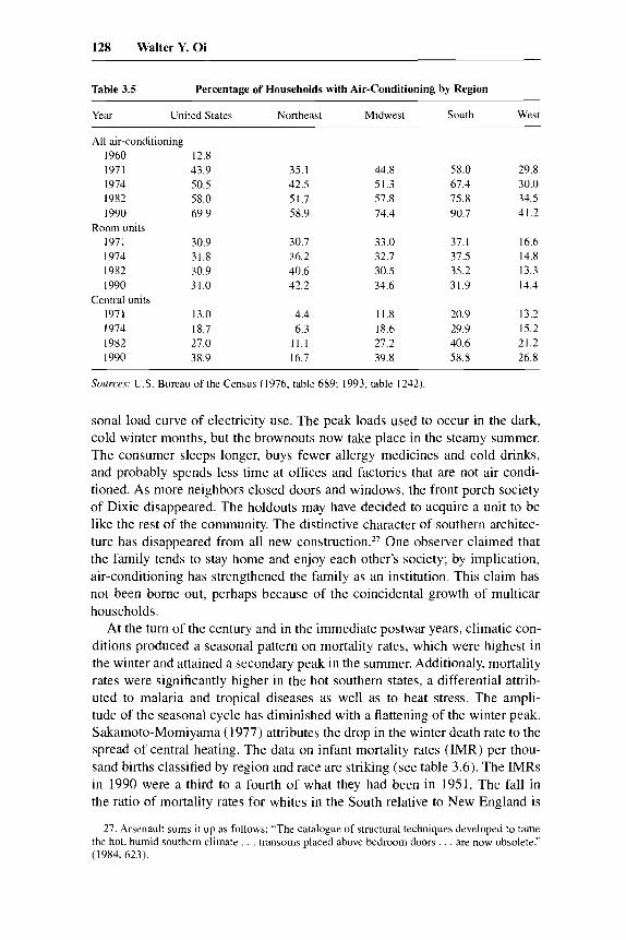
Although the sales to commercial establishments were important, the residential market held the promise of truly large returns. Carrier recognized this and introduced a room air conditioner in 1931. But sales were disappointing and were discontinued. At the end of World War 11, the situation looked good, incomes were high, the costs of producing the apparatus had come down, and electricity was cheap. However, it was not the Carrier Corporation but General Electric, Chrysler, and Frigidaire who introduced room units in 1950. By 1965, 12.8 percent of all households owned an air-conditioning unit. The diffusion was rapid, reaching nearly 70 percent of all households by 1990. The data in table 3.5 reveal some obvious regional differences: 90.7 percent of southern households had air-conditioning compared to only 41.2 percent in the West. Notice that the percentage with a room unit actually declined in the South, where more households installed central air. The rapid diffusion of air- conditioning in both the commercial and the residential sectors shifted the sea-

128 Walter Y. Oi

Table 3.5 Percentage of Households with Air-conditioning by Region

Year United States Northeast Midwest South West

All air-conditioning 1960 12.8 1971 43.9 1974 50.5 1982 58.0 I990 69.9

1971 30.9 1974 31.8 I982 30.9 1990 31.0

1971 13.0 I974 18.7 1982 27.0 I990 38.9

Room units

Central units

35.1 42.5 51.7 58.9

30.7 36.2 40.6 42.2

4.4 6.3

11.1 16.7

44.8 51.3 57.8 74.4

33.0 32.7 30.5 34.6

11.8 18.6 27.2 39.8

58.0 67.4 75.8 90.7

37.1 37.5 35.2 31.9

20.9 29.9 40.6 58.8

29.8 30.0 34.5 41.2

16.6 14.8 13.3 14.4

13.2 15.2 21.2 26.8

Sources: U S . Bureau of'the Census (1976, table 689; 1993, table 1242)

sonal load curve of electricity use. The peak loads used to occur in the dark, cold winter months, but the brownouts now take place in the steamy summer. The consumer sleeps longer, buys fewer allergy medicines and cold drinks, and probably spends less time at offices and factories that are not air conditioned. As more neighbors closed doors and windows, the front porch society of Dixie disappeared. The holdouts may have decided to acquire a unit to be like the rest of the community. The distinctive character of southern architec- ture has disappeared from all new con~truct ion.~~ One observer claimed that the family tends to stay home and enjoy each other's society; by implication, air-conditioning has strengthened the family as an institution. This claim has not been borne out, perhaps because of the coincidental growth of multicar households.

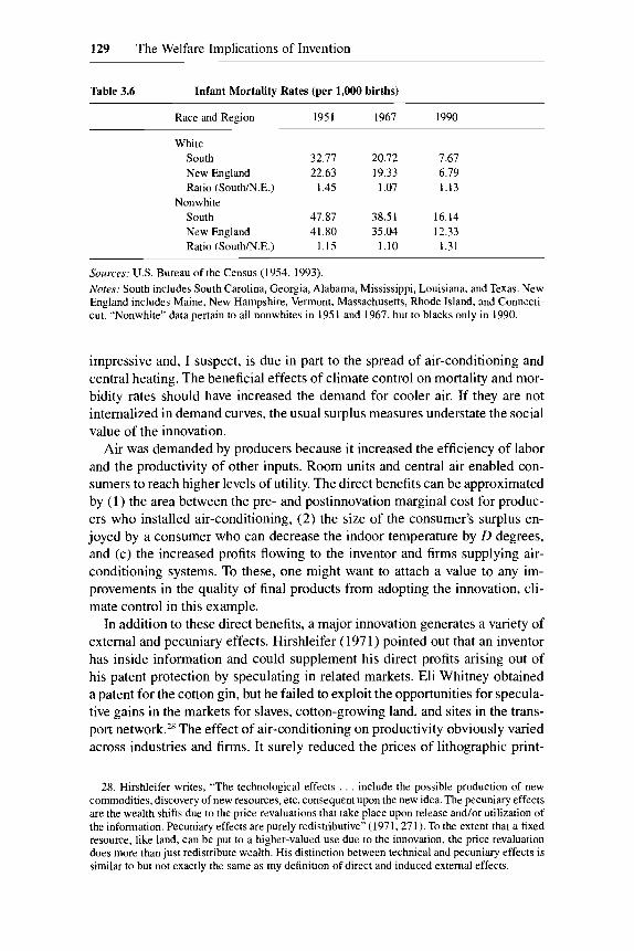
At the turn of the century and in the immediate postwar years, climatic conditions produced a seasonal pattern on mortality rates, which were highest in the winter and attained a secondary peak in the summer. Additionaly, mortality rates were significantly higher in the hot southern states, a differential attrib- uted to malaria and tropical diseases as well as to heat stress. The ampli- tude of the seasonal cycle has diminished with a flattening of the winter peak. Sakamoto-Momiyama (1977) attributes the drop in the winter death rate to the spread of central heating. The data on infant mortality rates (IMR) per thou- sand births classified by region and race are striking (see table 3.6). The IMRs in 1990 were a third to a fourth of what they had been in 1951. The fall in the ratio of mortality rates for whites in the South relative to New England is

27. Arsenault sums it up as follows: "The catalogue of structural techniques developed to tame the hot, humid southern climate . . . transoms placed above bedroom doors . . . are now obsolete." (1984. 623).


Table 3.6 Infant Mortality Rates (per 1,000 births)

Race and Region 1951 1967 1990

White south 32.77 20.72 7.67 New England 22.63 19.33 6.79 Ratio (S0uthN.E.) 1.45 1.07 1.13

South 47.87 38.5 1 16.14 New England 41.80 35.04 12.33 Ratio (South/N.E.) 1.15 1.10 1.31

Nonwhite

Sources: U.S. Bureau of the Census (1954, 1993). Nores: South includes South Carolina, Georgia, Alabama, Mississippi, Louisiana, and Texas. New England includes Maine, New Hampshire, Vermont, Massachusetts, Rhode Island, and Connecti- cut. “Nonwhite” data pertain to all nonwhites in 1951 and 1967, but to blacks only in 1990.

impressive and, I suspect, is due in part to the spread of air-conditioning and central heating. The beneficial effects of climate control on mortality and mor- bidity rates should have increased the demand for cooler air. If they are not internalized in demand curves, the usual surplus measures understate the social value of the innovation.

Air was demanded by producers because it increased the efficiency of labor and the productivity of other inputs. Room units and central air enabled consumers to reach higher levels of utility. The direct benefits can be approximated by (1) the area between the pre- and postinnovation marginal cost for producers who installed air-conditioning, ( 2 ) the size of the consumer’s surplus enjoyed by a consumer who can decrease the indoor temperature by D degrees, and (c) the increased profits flowing to the inventor and firms supplying air- conditioning systems. To these, one might want to attach a value to any improvements in the quality of final products from adopting the innovation, climate control in this example.

In addition to these direct benefits, a major innovation generates a variety of external and pecuniary effects. Hirshleifer (197 1) pointed out that an inventor has inside information and could supplement his direct profits arising out of his patent protection by speculating in related markets. Eli Whitney obtained a patent for the cotton gin, but he failed to exploit the opportunities for specula- tive gains in the markets for slaves, cotton-growing land, and sites in the transport network.28 The effect of air-conditioning on productivity obviously varied across industries and firms. It surely reduced the prices of lithographic print-

28. Hirshleifer writes, “The technological effects . . . include the possible production of new commodities, discovery of new resources, etc. consequent upon the new idea. The pecuniary effects are the wealth shifts due to the price revaluations that take place upon release and/or utilization of the information. Pecuniary effects are purely redistributive” (1971,271). To the extent that a fixed resource, like land, can be put to a higher-valued use due to the innovation, the price revaluation does more than just redistribute wealth. His distinction between technical and pecuniary effects is similar to hut not exactly the same as my definition of direct and induced external effects.

130 Walter Y. Oi

ing, cloth, cigars, and dried macaroni. Since there are economies of scale in cooling air, it favored large firms and stores. Its presence also affected other industries. The construction of high-rise office and apartment buildings and the development of high-speed elevators came after air-conditioning and, I suspect, would not have taken place without it. The early mainframe computers required climate control to be efficiently operated, especially in hot, humid climates. The value of land in Manhattan, Hong Kong, and Chicago would be significantly lower in the absence of air-conditioning. The market demand curves for air-conditioning do not fully capture the external benefits enjoyed by third parties, such as an office in the World Trade Center, an IBM 650 computer to estimate a logistic growth curve, or a movie in August. In the spirit of Russell Baker, it is my understanding that as late as 1970, federal civil servants were allowed to go home if the temperature exceeded 90 degrees, which by the usual presumption should have reduced the output of the government.

The air-conditioning of cars and trucks offers another example of benefits that were not fully anticipated. We knew how to cool a car in 1930 but had to wait until after the war before this improvement to Carrier's basic invention was commercially introduced. In 1965, only 10 percent of all new cars had factory-installed air conditioners, but the penetration rate climbed to 80.6 percent in 1982 and to 91.9 percent in 1990.29 Driving today is not only more comfortable, but safer. The fatal-accident rate per million vehicle miles fell from 7.59 in 1950 to 1.56 in 1992. When temperature and humidity are high, drivers are less alert, peripheral vision deteriorates, and response rates tend to increase. Theory suggests that when more cars are air conditioned, accident rates ought to fall.'O In passing, driving is less onerous in an air-contitioned vehicle which may, in part, account for the rapid growth of long-haul trucking.

In 1940,3 1.6 percent of all Americans resided in the South. The destruction of employment opportunities, due in large measure to technical advances in agriculture (of which the most significant was probably the mechanical cotton picker), prompted an out-migration to the North and West. The share of the population living in the South fell to 30.7 percent in 1960, reaching a trough around 1965. At least two factors were responsible for the reversal of the out- migration. First, the labor force participation rate of older men decreased, and many chose to retire in the South. The ability to live year-around in a cool, comfortable home must surely have influenced the choice of a retirement site. Second, air-conditioning eliminated the productivity penalty of locating an establishment in the South. The demand for labor expanded, and the per capita income of southerners rose from 76.4 percent of the average for the country as

29. Motor Vehicle Manufacturers Association (1991,38). The percentage of trucks with factory- installed air conditioners was 52.6 percent in 1982 and 81.4 percent in 1990.

30. The effect of temperature on injury frequency rates at the workplace was established by Vernon (1921). References to other studies that find a positive relation between high temperatures and accident rates in general can be found in Surry (1971, 93). I do not claim that air-conditioning is a major factor in the decline in fatal auto accident rates, but It surely deserves to be studied.


Table 3.7 Population and Personal Income by Region

1950 1970 1990

Population (in thousands) East 39,478 North 44,460 South 47,197 West 20,190 United States 15 1,325

Per capita personal income (constant 1987 dollars)

East 8,106 North 7.528 South 5,384 West 7,801 United States 7,046

Regional per capita income (percentage of US. )

East 115.0 North 106.8 South 76.4 West 110.7 Unitcd States 100.0

49.04 I 5657 1 62,795 34,805

203,2 I2

12,072 10,905 9,327

1 1,490 10,799

111.8 101.0 86.4

106.4 100.0

50,809 59,669 85,446 52,786

248,710

18,916 15,876 14,739 16,821 16,307

116.0 97.4 90.4

103.2 100.0

Sources: U S . Bureau of the Census (1995, 461, table 713) and selected issues of the Bureau of Economic Analysis’ Survey of Currenr Business. Nores: North corresponds to Midwest in previous tables, East to Northeast.

a whole to 90.4 percent; see table 3.7. The trend in relative per capita income was in the opposite direction for those residing in the North; per capita income there fell to 97.4 percent of the U.S. average in 1990. It is not surprising that more people are attracted to the South where they can control the indoor climate and command a higher relative income. You can drive to an air- conditioned workplace in an air-conditioned car, shop in an air conditioned mall, and watch a ball game in an air-conditioned dome stadium. A third of the farm tractors have air-conditioned cabs, and in Chalmette, Louisiana, aluminum workers walk around with portable air conditioners strapped to their belts (see Arsenault 1984,613). Fifteen years ago, Frank Trippett opined that people no longer think of interior coolness as an amenity but as a necessity.j’ The rejuvenation of Dixie could not have taken place without Willis Carrier’s invention. The nearly ubiquitous presence of air-conditioning is responsible for higher productivity, more comfortable homes, and longer life expectancies. I initially thought that this innovation would be adopted and imitated in other countries with climates similar to that in the deep South. However, the private

3 1. Arsenault also reports (1984, 614) that at the 1980 Governors’ Conference, Governor Rich- ard W. Riley of South Carolina insisted that the federal assistance program should operate on the assumption that air-conditioning a home in the South was no less essential than heating a home in the North. Energy tax credits should be made available to all.

132 Walter Y. Oi

value of air-conditioning is inversely related to the price of the apparatus and the price of electricity. High energy taxes reduce the demand for air- conditioning. The consequences are lower labor productivity, less work in the hot summer months, uncomfortably hot and humid homes, and poor health.

3.6 Knowledge and Novelty

Invention, defined as “a new combination of available knowledge,” can sometimes be produced, but in other instances it is the result of luck. The production of knowledge differs from the relation between output and inputs which is the familiar production function in a neoclassical theory of value. There is more uncertainty in creating a new product. One can point to numer- ous cases where substantial outlays have failed to solve a problem or to discover a patentable product. Prospecting for an oil well or searching for a job are analogous, in some ways, to searching for a new product or process. But while the cost of a dry hole is part of the full cost of supplying petroleum, each invention is unique, and there is no “knowledge industry” to absorb the costs of unsuccessful inventive activities. In spite of this difference, some have tried to estimate the expected cost by relating R&D expenses to the output of patented inventions. The limitations of these estimates were discussed in section 3.3. Additionally, patented inventions include truly new products and ideas as well as imitations and improvements; that is, patents and patent applications are not homogeneous. Arrow suggests that the cost of an invention (dis- covering a new idea) is stochastic and depends on the stage of the economy’s development: “The set of opportunities for innovation at any one moment are determined by what the physical laws of the world really are and how much has already been learned and is therefore accidental from the viewpoint of economics” (1969, 35). A patent award is only the first step in producing an innovation. A majority of patents are stillborn and never make a debut in the market. The economic lives of the new entrants are threatened by the creation of new knowledge.

A new product may have to be modified and improved before it can be introduced. Information has to be disseminated to potential customers. A distribution channel has to be established. These are some of the components that belong to the “D’ in R&D costs. The lag between invention and innovation can be long, often exceeding seventeen years. An inventor can shorten the length of this lag and raise the probability of a successful entry to the market by incurring more R&D costs.

The pace of technical progress can allegedly be stimulated by a policy that subsidizes R&D expenditures, possibly via tax credits. A blanket subsidy cannot differentiate among inventors or types of expenditures. A firm searching for a sugar substitute (when sugar is protected by import quotas) would receive the same rate of subsidy as one incurring R&D costs to discover a biodegrad- able plastic. Would the same rate of subsidy be granted for test-marketing a new brand of cat food and paying for research scientists? A regulatory agency


would have to be created if we wanted to subsidize only the deserving research projects. This agency would have to promulgate something resembling an industrial policy. A subsidy would expand R&D expenditures, resulting in a higher average cost of an invention. Products would be likely to reach the market earlier, more would be spent on unsuccessful ventures, and inventors would have less incentive to cut their losses by stopping dubious projects. It must also be remembered that products are like people and penguins, they have uncertain and finite lives. The discovery of a new alloy could destroy the value of a tin mine along with the R&D capital invested in developing more-efficient tin- mining equipment. The inability to forecast the length of a product’s life cycle necessarily increases the risk confronting inventors and innovators. It is not at all obvious that society would realize a positive rate of return on the incremen- tal R&D expenditures attracted by a subsidy program.

The social returns to a major innovation (like the telephone, penicillin, the computer, or even air-conditioning) far exceed the sum of consumer’s and producer’s surpluses, the private returns accruing to the parties directly involved in the market for the new product or process. A major innovation affects third parties, changes preferences, and opens the way for technical advances in other sectors. The prices of cigars and cloth were lower because of air-conditioning. The diffusion of air-conditioning increased the profitability of engaging in research that led to high-rise office buildings, high-speed elevators, and mainframe computers. Carrier’s patent had expired long before air-conditioning was introduced to the residential market. The spread of air-conditioning reversed the outflow of people and jobs from the South. A consumer’s surplus measure of the value of driving in an air-conditioned vehicle or shopping in comfort presumes that one can identify a stable demand for the new product, air- conditioning in this example. However, for some new products, experience teaches consumers about additional uses which shift the demand for the new product. The situation for a really successful new good is similar to the de gustibus model of Stigler and Becker (1977). As consumers learned more ways to utilize climate control, they demanded more of it, resulting in a larger ex post demand and consumer’s surplus. The economic life of a successful innovation will almost certainly exceed the statutory life of the patent. The original inventor may continue to realize supernormal returns because she enjoys any advantages associated with being the first producer and probably has the ability to stay ahead of any competitors in terms of product improvements. A society can encourage more inventive activities by either subsidizing costs or enhanc- ing returns. When we know so little about the costs of invention and innovation (especially the dry ventures), it would seem wiser to consider policies that enhance the returns to inventors. This might be done by extending the patent life for a really novel invention to, say, twenty-five years and shortening it for an improvement or imitation to, say, five years. The patent office would have to make the distinction by reviewing the patent application to see how much it relies on existing knowledge. The merits of renewing patents for a fee should be studied. The objective is to increase the mean, especially the dispersion, of

134 Walter Y. Oi

returns to invention. If most inventors exhibit a utility function of wealth with an inflection point of the type posited by Friedman and Savage ( 1948), a larger dispersion of returns will increase the supply of inventive activity.’’ A policy that operates on incentives stands a better chance of success in promoting a faster pace of technical progress.

Technical progress can occur through the creation of new products or through the discovery of new techniques to produce the old list of products at lower costs. Consider an economy in which all progress takes the form of cost- reducing innovations. The memberc of this economy can enjoy an ever growing flow of consumption because more goods and services can be produced even with no increase in the quantity or quality of productive inputs. Firms simply acquire the knowledge to produce more corn, tallow, and gingham with the same workers and capital. Alternatively, we can imagine another economy in which progress entails the creation of new goods and services. The people in this economy are forced to adjust to novelty; they confront a continually changing catalogue of goods and services from which they can choose. More time and effort have to be allocated to learning about new foods, places to visit, and whether to buy a new plastic knee rather than to demand traditional medi- cal care to mend a wounded knee. Most of us do not have to choose between these two extreme faces of technical advance; we probably would like to get a mixture. Few of us would opt for the status quo economy. It would be a terribly dull life if innovations only reduced the costs of producing the same menu of goods and services that now populate our markets. People have revealed that they like new things. The uncertainty of what will become available in tomor- row’s market surely prompts many of us to put forth more effort today in order to acquire the wherewithal to get a ride on the supersonic jet or the opportunity to influence the outcome of a game via an interactive television set. Hilton noted that “An inventor has an incentive to maximize his claims to novelty” (1 97 1, 2 1 ). If the inventor can occasionally deliver on his claims, the welfare of society will continue to grow.

Appendix

Climate and Productivity: A First Approximation

Suppose that output is a function of labor and capital inputs as well as of temperature, T, which is a shorthand term for an index of air quality defined by temperature, humidity, cleanliness, and ventilation.

(‘41 1 X = f ( L , K , T ) .

32. The distribution of prizes in most state lotteries reveals a fairly large numher of small prizes (so that a significant number can say that they won something) and a few megaprizes that can be prominently announced on television and in the newspapers. If consumers exhibit a utility function with an inflection point, they will simultaneously purchase insurance and lottery tickets.


Suppose initially that temperature, like Meade’s atmosphere, is exogenous and affects output in a Hicks Neutral fashion.

( A l ‘ ) x = + ( T ) g ( L K ) ,

where +( T ) is a bell-shaped function attaining a maximum at some ideal, moderate temperature TM . A competitive firm operates over a cycle of two periods with temperature above the ideal in the first period, and TB below the ideal in the second period. The capital has to be the same in both periods, but the labor input can be adjusted given the temperature. Ignoring discounting, profits over a cycle of two periods are given by

(A21 n = p ( X , + X , ) - w(La + L B ) - 2rK.

When temperature affects productivity in a Hicks Neutral fashion, its impact can be analyzed by defining what I call temperature-adjusted prices. Let p a =

p + ( q ) denote the effective price in the hot period, while p B = p + ( T,) is the effective price in the cold period when the firm is obliged to accept the exogenous temperatures. If we normalize + ( T ) to equal unity at the ideal temperature, then pa < p , and p , < p . In equilibrium, labor’s MVP will be equated to the wage in each period, while the sum of capital’s MVP over the two periods is equated to its full-cycle price.

If hot weather leads to a larger decrement in productivity, +( T,) < +( T,) < 1, and p A < p , . Although labor’s MVP is equal to the common wage, g L , will be greater than g,,, an outcome that can only be achieved by hiring fewer workers in hot weather. However, the inability to vary capital over the cycle results in employing “too much” capital in the hot first period. The departures of temperature from the ideal climate, T,, raise production costs, leading to lower profits. Indeed, profits, in this base case, will be smaller, the larger are the temperature departures from the ideal.

Suppose that a technological innovation enables the firm to cool the indoor temperature to T, = T, - D at a cost of ( 4 + c,D) and to heat the plant in the cold period to an indoor temperature of = ( T , + I ) at a cost of (F, + c , l ) . The fixed and marginal costs of cooling and heating will depend on the size and insulation of the plant and on the nature of the production process. A bak- ery is costlier to cool than a warehouse. Profits now are a function of five decision variables { L , , L2 , K*, D , I ] , where D and I determine the indoor cli- m a t e ~ . ~ ~

33. The Sacket Wilhelm Company in Brooklyn wanted temperatures of 70 degrees in the winter and 80 degrees in the summer with a constant humidity of 55 percent. The optimum temperature for worker efficiency is around 67 degrees, but Wilhelm had to consider the effect of temperature on paper and paints.

136 Walter Y. Oi

(A4)

In equilibrium, the firm will satisfy conditions analogous to equations (A3a) and (A3b), wherep, = p+(T, ) replacesp, in the hot period, andp? = p + ( T , ) replaces p s . The optimal decrement in temperature in the hot period, D = r, - T,, is attained when the marginal benefit is equal to the marginal cooling cost, equation (A5a), provided that the increment to quasi-rent exceeds the total cooling cost, equation (A5b).

n = p ( X , + X , ) - w(L, + L 2 ) - 2rK* - F, - c,D - F, - c , l .

where AC is the increment in costs of hiring more labor and capital. A similar pair of conditions must hold if it pays the firm to increase the temperature in the cold second period. Remember that the cost parameters { F, , c,} for cooling depend on the size and insulation of the plant and have declined over time. More importantly, the effect of temperature on productivity, +( T ) , varies across industries. The gain in productivity from cooling and humidifying the air was undoubtedly greater for a textile mill than for a bottling plant. The installation of cooling and heating equipment raises the productivity parame- ter, +( T ) . As a consequence, the effective product prices climb, ( p , > p,, , p z > p , ) , prompting the firm to expand output. If a majority of firms in an industry find that controlling the indoor climate is profitable, the price of the product will fall, to the benefit of consumers.

Temperature and Labor Productivity: A Second Approximation

Suppose that the labor input is the product of person hours ( H ) times the efficiency per hour which is a function of the temperature; L = E( T ) H, where E( T ) attains a maximum at some ideal, moderate temperature. Assume that the exogenous outdoor temperature in the absence of air-conditioning is above this ideal, T, > TM . A competitive firm chooses labor hours and capital { H , K ) to maximize profits.

(-46) n = pf[E(T,)H, K ] - w H - r K .

Let E = E(T,) denote labor efficiency with the unregulated temperature. Profits no are at a maximum when the MVP of hours and capital are equated to their respective prices.

Since E‘ ( T ) < 0, firms located in hotter places confront a higher “price” per efficiency unit of labor. The capital-to-labor ratio, K I L = KIEH, will be higher, but the capital-to-hours ratio, K I H , will be higher if and only if the


elasticity of substitution is greater than one. More importantly, if the hourly wage w is the same for all, a firm in a hot place faces a higher price for an efficiency unit of labor and is at a cost disadvantage relative to competitors located in milder climates.

Suppose now that the firm can reduce the temperature by D degrees, to T* = ( T , - D ) at a cost of ( F + c D ) . The firm will install air-conditioning if the increment to quasi-rent exceeds the total cooling cost.

(A8a) p(X* - X ) - AC > F + cD,

where X* and D are chosen to equate marginal gains to marginal costs.

(A8b) pEf , = w, p f , = r, -E' (T, - D)Hpf , = c.

Cooling has an effect similar to a labor-saving innovation. The relative price of labor ( w l E * r ) falls, the demand for capital K increases, and the firm supplies more output to the market, X* > X . The increment to labor productivity, E* = E( T, - D ) , depends on the properties of E( T ) and on the marginal cost of cooling, c. The model can be extended to demand cooling in a hot period and heating in a cold period, but this extension is not undertaken here.

Household Demands for Heating and Cooling

Comfort is surely a function of the indoor temperature and humidity, which could be included as an argument of the utility function alongside a consumption good, U ( X , T) . Friedman (1987) argued that if heat loss is mainly due to conduction (rather than radiation or convection), the total cost of heating a house is a linear function of the gap between the desired indoor and exogenous outdoor temperatures.

iA9) TC = F + c (T - To),

where F is the fixed monthly cost and c is the unit cost of raising the indoor temperature by one degree. Utility is maximized when the marginal rate of substitution of indoor temperature for consumption (taken to be the numeraire) is equated to the marginal cost of raising T by one degree.

Remember that a warmer indoor temperature raises utility, that is, U,, > 0. The heating-cost parameters { F, c } depend on the size of the house, the price of energy, and the structure of the home. Specifically, more outlays for insulation z increase the fixed cost F but reduce the marginal heating cost, c = c( z ) with c' (z) < 0. If consumers in different locations have the same tastes, and if wages adjust to equalize total utilities across locations, persons in colder climates will spend more on insulation and hence confront a lower marginal cost of raising the temperature. They accordingly maintain their homes at a

138 Walter Y. Oi

higher indoor temperature. It is a neat model that can parsimoniously explain why houses in Chicago are warmer in the winter than houses in Los Angeles even though the former entail a higher total heating cost. This model has to be extended in at least two directions for a residential demand for cooling to be derived. First, the cost function has to be amplified. Second, the interaction between indoor temperature and home size has to be made explicit in a manner analogous to the household production model of Becker (1965).

The cost of climate control can be decomposed into an avoidable fixed cost plus a variable operating cost that is assumed to be a linear function of the desired temperature decrement, D = ( T - T ) . The fixed cost is proportional to the price of the apparatus 4, which, in turn, is a function of the volume of air to be chilled and the cost of the compressor, ducts, and other equipment, while the unit cooling cost is a function of the structural charactersitics and the price of electricity P, .

where r is the interest rate and T is the expected life of the apparatus. Utility is inversely related to the indoor temperature, U ( X , r), where UTE < 0. The demands for corn and cooling degrees { X , D = T - 7;) are determined by a budget constraint and the equality of the marginal rate of substitution to the relative price of cooling.

(A12a) X + F + c(T0 - T ) = M,

(A12b) - p) = c(Pe) .

Let w = w( D ) denote the marginal offer price that a consumer is prepared to pay for the Dth degree of cooling. The consumer’s surplus when D* is the optimal decrement in temperature isi4

D*

(A131 CS = w ( D ) d D - c(P<,)D*

A consumer will incur the avoidable fixed cost if it is less than the consumer’s surplus from obtaining a cooler home; that is, he will install air-conditioning if F < CS. The fraction of consumers who find that this inequality holds and hence install air-conditioning will climb over time as the price of the apparatus falls, thereby reducing the avoidable fixed cost F, or as the price of electricity declines, thereby increasing the consumer’s surplus CS.

34. The optimal bundle {X*, D* = T ~ T : } is obtained by solving equations (A12a) and (A12b). The marginal offer price need not be a strictly declining function of D. The consumer may not be willing to pay much for the first few degrees of cooling from an outdoor temperature of = 85 degrees to, say, T = 82 degrees, but in the neighborhood of equilibrium, it seems safe 10 assume that dwldD < 0.


The temperature decrement, D = ( T - T ) , the difference between outdoor and indoor temperatures, tacitly assumes a given volume of air to be chilled by D degrees. If V is the volume of air, the quantity of climatically controlled air demanded by a household can be approximated by Q = DV When air- conditioning was initially introduced to the residential market, most consumers purchased room units which entailed a smaller avoidable fixed cost F but a higher marginal cooling cost c(%). These room units also cooled a smaller quantity of air. As incomes rose and as the price of the apparatus and the price of electricity Pe fell, consumers expanded their demand for chilled air, Q = DV by installing central air-conditioning systems. Finally, if the consumption good X is disaggregated, a change in the indoor temperature will differentially affect the demands for particular goods. The ability to reduce the inside temperature from 85 to 65 degrees has to affect the demands for soft drinks, salads, and electric fans. Many of us can remember an occupant of the White House who would turn up the air conditioner in order to enjoy an eve- ning before a crackling wood fire in the summer.

References

Alchian, A. A. 1959. Costs and outputs. In The allocation of economic resources, ed.

Arrow, K. J. 1969. A classificatory note on the production and transmission of techno-

Arsenault, Raymond. 1984. The end of the long hot summer: The air conditioner and

Asher, Harold. 1956. Cost-quantity relationship in the airframe industry. Santa Monica,

Bailey, N. T. J. 1957. The mathematical theory of epidemics. New York: Charles Griffin. Baker, Russell. 1978. No sweat. New York Times Magazine, 9 July. Quoted in Arsenault

1984,605. Becker, G. S. 1965. A theory of the allocation of time. Economic Journal 75 (Septem-

ber): 493-517. Booz, Allen, and Hamilton. 1971. Management ofnew products. New York: Booz, Al-

len, and Hamilton, Inc. Chaney, Paul K., Timothy M. Devinney, and Russell S. Winer. 1991. The impact of new

product introduction on the market value of firms. Journal of Business 64:573-610. Coale, Ansley, and Donald McNeil. 1972. The distribution by age of the frequency of

first marriage in a female cohort. Journal of the American Statistical Association 67 (December): 743-49.

Coase, Ronald H. 1972. Durability and monopoly. Journal of Law and Economics

Council of Economic Advisers. 1988. Economic report of the president. Washington,

Davidson, J. Hugh. 1976. Why most new consumer brands fail. Haward Business Re-

Davidson, J. P., P. S. Florence, B. Gray, and N. Ross. 1958. Productivity and economic

M. Abramovitz, 23-40. Stanford, Calif.: Stanford University Press.

logical knowledge. American Economic Review, Papers 29 (May): 29-35.

southern culture. Journal of Southern History 50, no. 4 (November): 597-628.

Calif.: RAND. 1 July.

145: 143-49.

D.C.: Government Printing Office.

view 54 (March/April): 117-22.

Incentives. London: Allen and Unwin.

140 Walter Y. Oi

Denison, E. F. 1962. Sources of economic growth in the United States and the alterna- tives before us. New York: Committee for Economic Development.

Enos, J. 1962. Invention and innovation in the petroleum refining industry. In The rate and direction of inventive activity: Economic and social factors, 299-322. National Bureau of Economic Research Conference series, vol. 13. Princeton, N.J.: Princeton University Press.

Evenson, Robert. 1993. Patents, R&D, and invention potential: International evidence. American Economic Review, Papers 83 (May): 463-68.

Evenson, Robert E., and Yoav Kislev. 1975. Agricultural research and productivity. New Haven, Conn.: Yale University Press.

Fisher, F. M., and K . Shell. 1968. Taste and quality change in the pure theory of the true cost of living index. In Value, capital, and growth, ed. J. N. Wolfe, 97-139. Chicago: Aldine Publishng.

Florence, P. Sargant. 1924. The economics ojfutigue and unrest: The efJiciency of la- bour in English and American Industry. New York: Henry Holt.

Freeman, Christopher. 1991. The economics of industrid innovation. 2d ed. Cambridge, Mass.: MIT Press.

Friedman, David. 1987. Cold houses and warm climates and vice versa: A paradox of rational heating. Journal of Political Economy 95 (October): 1089-97.

Friedman, M., and L. J. Savage. 1948. The utility analysis of choices involving risk. Journal of Political Economy 56 (August): 279-304.

Griliches, Zvi. 1957. Hybrid corn: An exploration in the economics of technological change. Econometrica 25 (October): 501-22.

. 1990. Patent statistics as economic indicators: A survey. Journal of Economic Literature 28 (December): 1661-707.

Grossman, G. M., and E. Helpman. 1991. Endogenous product cycles. Economic Jour- nal 10 1 : 12 14-29.

Helpman, Elhanan. 1993. Innovation, imitation, and intellectual property rights. Econo- metrica 61 (November): 1247-80.

Hicks, John R. 1959. Revision of demand theory. London: Oxford University Press. Hilton, George W. 1971. Cable car in America. Berkeley, Calif.: Howell-North Books. Hirshleifer, Jack. 197 1 . The private and social value of information and the rewards for

inventive activity. American Economic Review 6 1 (September): 561-74. Huntington, Ellsworth. 1924. Civilization and climate. 3d ed., 13-16, 80-108. New

Haven, Conn.: Yale University Press. Ingels, Margaret. 1952. Willis Haviland Carrier; father of air conditioning. Garden City,

N.Y.: Country Life Press. Jewkes, John, David Sawers, and Richard Stilleman. 1958. The sources of invention.

New York: St. Martin’s Press. Kuznets, Simon. 1962. Inventive activity: Problems of definition and measurement. In

The rate and direction of inventive activity: Economic and social factors, 19-5 1. National Bureau of Economic Research Conference series, vol. 13. Princeton, N.J.: Princeton University Press.

Lebergott, Stanley. 1993. Pursuing happiness. Princeton, N.J.: Princeton University Press.

Mansfield, E. 1966. Technological change: Measurement, determinants, and diffusion. In Studies of the employment impact of technological change. Vol. 2. Washington, D.C.: Government Printing Office.

Moore, Henry Ludwell. [ 191 11 1967. Laws of wages, an essay in statistical economics. Reprint, New York: Augustus M. Kelley Publishers.

Motor Vehicle Manufacturers Association. 199 1. Motor vehicle facts andfigures, 1991. Detroit, Mich.: Motor Vehicle Manufacturers Association of the United States.

Mowery, David C. 1988. The diffusion of new manufacturing technology. In The impact


of technological change on employment and economic growth, ed. Richard M. Cyert and David C. Mowery, 48 1-509. Cambridge, Mass.: Ballinger Publishing.

Oi, W. Y. 1991. Low wages and small firms. In Research in labor economics, ed. R. Ehrenberg. Vol. 12, 1-39. Greenwich, Conn.: JAI Press.

Romeo, A. A. 1975. Interindustry and interfirm differences in the rate of diffusion of an innovation. Review of Economics and Statistics 57:311-19.

. 1977. The rate of imitation of a capital embodied process innovation. Econom- ica 44:63-69.

Rosenberg, Nathan. 1982. Inside the black box: Technology in economics. New York: Cambridge University Press.

Rothbarth, E. 1941. The measurement of changes in real income under conditions of rationing. Review uf Economic Studies 8: 100-107.

Sakamoto-Momiyama, Masako. 1977. Seasonality in human mortality. Tokyo: Univer- sity of Tokyo Press.

Samuelson, Paul Anthony. 1948. Foundations ofeconomic analysis. Cambridge, Mass.: Harvard University Press.

Scherer, F. M. 1965. Firm size, market structure, opportunity and the output of patented inventions. American Economic Review 55 (December): 1097-1 123.

Stigler, George J. 1968. A note on patents. In The organization ofindustry. 122-25. Chicago: University of Chicago Press.

Stigler, G. J., and G. S. Becker. 1977. De gustibus non est disputandum. American Eco- nomic Review 67 (March): 76-90.

Stokey, Nancy L. 1979. Intertemporal price discrimination. Quarterly Journal of Eco- nomics 94:355-71.

Surry, Jean. 197 1. Industrial accident research. Toronto: Labor Safety Council. May. U.S. Bureau of Labor Statistics. 1983. Handbook of labor statistics. Washington, D.C.:

U S . Bureau of the Census. 1954. Statistical abstract of the United States. Washington,

. 1976. Statistical abstract ofthe United States. Washington, D.C.: Government

. 1987. Census of manufactures. Washington, D.C.: U.S. Bureau of the Census.

. 1993. Statistical abstract ofthe United States. Washington, D.C.: Government

. 1995. Statistical abstract of the United States. Washington, D.C.: Government

Usher, Dan. 1964. The welfare economics of invention. Economica 31 (August):

Vernon, H. M. 1921. Industrial fatigue and ejjiciency. London: Routledge.

Government Printing Office.

D.C.: Government Printing Office.

Printing Office.

Printing Office.

Printing Office.

279-87.

This Page Intentionally Left Blank

the welfare implications of invention - core.ac.uk · however, the upward trend ... if income...

Documents