the world bank latin america and the …pubdocs.worldbank.org/en/780311492653985192/p... ·...

The World Bank LATIN AMERICA AND THE CARIBBEAN REGION

OFFICE OF THE CHIEF ECONOMIST GLOBAL PRACTICE OF TRANSPORT AND ICT

Road Networks, Accessibility, and Resilience: The Cases of Colombia, Ecuador, and Peru

An LCR Regional Study Cecilia Briceño-Garmendia, Harry Moroz, and Julie Rozenberg

With: Xijie Lv

Siobhan Murray Laura Bonzanigo

June 30th, 2015

1

Acknowledgements This study was sponsored by the Chief Economist’s Office in the Latin America and the Caribbean Vice-Presidency of the World Bank under the series of Regional Studies. The core team of the study includes Cecilia Briceño-Garmendia (TTL, GTIDR), Harry Moroz (co-TTL, GTIDR); Julie Rozenberg (GCCCE); Xijie Lv (GTIDR); Siobhan Murray (DECSM); and Laura Bonzanigo (GCCCE). The team is particularly thankful to Marianne Fay for her useful comments, guidance, and support throughout the writing and conceptualization of the report. Special thanks also go to peer reviewers Andreas Dietrich Kopp and Baher El-Hifnawi; and to Augusto de la Torre, Daniel Lederman, Jose Luis Irigoyen and Aurelio Menendez for their overall supervision. The team also is also very grateful for the timely support and comments provided by Rodrigo Archondo-Callao and Alberto Nogales (HDM-4); Henry Bofinger (airports); Brian Blankespoor (GIS); Daniel Benitez, Anca Dumitrescu, Eric Lancelot, Gregoire Gauthier, Satoshi Ogita and Maria Marcela Silva (transport operations and alternative interventions); Frederico Ferreira Fonseca Pedroso (disaster risk management); and Simon Ellis (road assets management). The team had significant assistance gathering data. Mauricio Cuellar and Camila Rodriguez Hernandez were instrumental to grant access to data for Colombia. Fernando Orduz of the Inter-American Development Bank was extremely gracious in sharing data on Ecuador’s road network. Patricia Lopez Martinez worked assiduously in Ecuador to help us locate this data. For Peru, the team benefited of a very productive collaboration with MINCETUR, the Ministry of Transport and Provias Decentralizado. Finally, the team would like to thank for their comments and suggestions the participants of workshops held in Lima in November 2014 and April 2015; a seminar held during the Transport and ICT Forum sponsored by the Road Asset Management Global Solution Group in April 2015; a workshop sponsored by the Green Transport Community of Practice in May 2015; and a half-a-day seminar organized jointly by the Climate Change Vice Presidency and the Transport and ICT Global Practice to explore areas for collaboration and operationalization of innovative methodologies.

2

Contents

I. PART 1: Overview, Methodology and Data, and Scope ........................................................................ 5

A) Overview ........................................................................................................................................... 5

B) About this Study ................................................................................................................................ 9

The Lay of the Land: The Landscape of the Pilot Countries ................................................................ 11

C) Methodology ................................................................................................................................... 13

i. Accessibility and Its Components ........................................................................................... 17

ii. Defining Accessibility .............................................................................................................. 17

iii. Measuring Accessibility ........................................................................................................... 18

iv. Accessibility and the Gravity Model ........................................................................................ 21

D) Data ................................................................................................................................................. 25

v. The GIS Road Network ............................................................................................................ 25

vi. Geographic and Topographic Data ......................................................................................... 31

vii. Economic Data .................................................................................................................... 33

viii. Social Data ........................................................................................................................... 37

ix. Natural Hazards ....................................................................................................................... 38

E) Combining Engineering with Geography to Calculate Road User Costs ......................................... 39

i. Teasing out the Power of GIS using Engineering Estimates: HDM-4 ...................................... 39

ii. Characterizing the Road Networks ......................................................................................... 41

II. PART 2: Spatial Disparities through the Accessibility Lens ................................................................. 47

A) Characterizing Accessibility: Engineers and Economists Working Together .................................. 48

B) Challenges for Achieving Good Accessibility ................................................................................... 54

i. Geography and Accessibility ................................................................................................... 54

ii. Population and Accessibility ................................................................................................... 56

iii. Income and Accessibility ......................................................................................................... 57

C) Drivers of Accessibility .................................................................................................................... 58

i. Social Exchanges ..................................................................................................................... 58

ii. Markets and Accessibility ........................................................................................................ 59

III. PART 3: Criticality of Corridors through the Accessibility Lens ....................................................... 59

A) Least-cost Routes and Indicative Corridors .................................................................................... 60

B) Measurements of Criticality ............................................................................................................ 62

i. Assessing Criticality for Ecuador Network .............................................................................. 66

ii. Assessing Criticality for Colombia Network ............................................................................ 68

3

iii. Assessing Criticality for Peru Network .................................................................................... 70

IV. PART 4: Decision Framework for Policy Makers—Increasing Reliability ........................................ 72

A) Trade-off between Reliability and Cost: A “Robust” Cost-effectiveness Analysis ...................... 74

Reliability as Minimum Network Costs ............................................................................................... 74

Analyzing the Trade-offs ..................................................................................................................... 75

B) Exposure to Floods: Colombia, Ecuador, and Peru ......................................................................... 75

C) Policy Options to Increase Resilience to Floods: The Case of Peru ................................................ 79

Expected Annual Losses ...................................................................................................................... 80

Possible Interventions ......................................................................................................................... 83

V. CONCLUSIONS AND APPLICATIONS .................................................................................................... 88

VI. References ...................................................................................................................................... 93

VII. Annexes ......................................................................................................................................... 102

4

I. PART 1: Overview, Methodology and Data, and Scope

A) Overview

High transport costs are among the most disruptive factors contributing to weak linkages between markets. In Latin America—where economies rely heavily on commodities1 and on economic and demographic patterns developed around urban clusters often far from dispersed rural populations2—economic activity and population mobility depend to a great extent on transport. Nearly two-thirds of Latin American exports are perishable or logistics intensive compared to less than 20 percent in the Organisation for Economic Co-operation and Development (OECD) (Moreira and others 2013; Andean Development Corporation 2013). Guasch and Kogan (2006) estimated logistics costs as a share of GDP in Latin America in the 1990s and found that they were two to four times the OECD’s costs. Freight costs are much more of a concern in Latin America than tariff costs, but receive substantially less attention in regional agreements (Andean Development Corporation 2013). The OECD (2013) computed the freight cost to tariff cost ratio between Latin America and its partners to be 9 to 1. This is over four times higher than the ratio of 2 to 1 observed between the United States and its partners (OECD 2013).Transport costs can represent up to 70 percent of the trade costs associated with intraregional exports and imports (Moreira and others 2013).

In the realm of domestic markets, the impact of high transport costs and the internal difficulties with moving crops and produce within a country to reach export outlets and distribution centers is alarming, though most of the evidence is anecdotal. In exporting pineapples to Europe, for example, Costa Rica loses 50 percent more produce on the trip to domestic distribution centers than from the distribution centers in Costa Rica all the way to Rotterdam (World Bank 2012). Inventory levels in the region have been higher than in the OECD by a factor of three (Gonzalez, Guasch, and Serebrisky 2007). Further, logistics costs in the LAC represent somewhere between 18 percent and 35 percent of a product’s value versus about 8 percent in the OECD countries (OECD 2013). A recent survey of trucking firms in Central America found numerous challenges, from aging truck fleets to high fuel costs, empty return trips, and long waiting times (OECD 2013; World Bank 2012). In the northern part of Rosario, Argentina, trucks line up for 15 kilometers (km) as a result of port and industrial expansion without accompanying improvements to traffic access (Serebrisky and Barbero 2006). In some parts of the region, the proportion of cargo carried by rail is 5 percent or less (Barbero 2011). In fact, the inadequacy of comodal transportation alternatives increases logistics costs 57 percent (OECD 2013).

High transport costs are in part a reflection of the poor accessibility of Latin America’s roads, rails, ports, and airports. The story of physical transport infrastructure quantity and quality in Latin America is mixed, though largely negative, across all modes. There are only 86 km of road and 1 km of rail for every 100 square kilometers (km2) of land area in Latin America, compared with 185 km and 4.3 km, respectively, in Europe and Central Asia. The region’s shipping connectivity is strikingly low. According to

1 For instance, the January 2015 edition of the World Bank Global Economic Prospects estimates that a one percentage point decline in China’s growth is associated with a 0.6 percentage point decline in growth in LAC (World Bank 2015). 2 Equality of opportunity and access to infrastructure is in great part a result of whether one lives in an urban or rural area (de Barro and others 2008; World Bank 2009). As Fay and Morrison (2007) points out, “Given that poverty is usually much higher in the countryside, lower rural access rates explain much (though by no means all) of the vast disparities in infrastructure coverage between rich and poor Latin Americans” (Fay and Morrison 2007).

5

estimates by the UN Conference on Trade and Development (UNCTAD), Latin America is the second-least-connected developing region, behind only Sub-Saharan Africa. An index of air connectivity shows LAC performing slightly better. Still, Latin America’ air connectivity is four times lower than that of North America and between one-third and one-half that of the Middle East and North Africa (MENA) and Europe and Central Asia (ECA).

Quality—or the perception of quality and reliability—is another widely used proxy, again admittedly flawed, for assessing transport services. On that token, Latin America’s transport scores raise concerns. The World Economic Forum’s (WEF’s) survey of infrastructure across the world shows Latin America’s infrastructure to be better than only that of South Asia or Sub-Saharan Africa across all transport modes with the exception of the rail sector, in which the region ranks last (figure 1). The average technical efficiency of Latin American ports—a measure of how well they turn inputs into outputs relative to the optimal—was found to be less than 50 percent between 1998 and 2007. This is ahead of Africa’s 30 percent but well below Europe’s 60 percent (Morales Sarriera and others 2013). Analysis of Latin American airports shows that they should be able to produce nearly twice as many passengers, tons of freight, and aircraft movements with the same number of employees, runways, and boarding bridges (Serebrisky 2012).

In all this story, the dominant transport mode for transporting goods and people within Latin America is roads. Passenger travel is dominated by vehicles with air making up about 10 percent of traffic and rail a negligible part (GTZ 2010). Forty-one percent of intraregional trade in terms of value travels by truck with a scant 0.70 percent traveling by rail (the figures are only slightly more favorable by volume) (ECLAC 2013).3

Roads in Latin America are in practice a blessing and a curse, on one hand providing access to jobs, markets, cities, and other countries. But on the other hand, roads can be the main barrier to achieving this access due to poor condition or location or, more simply, because they do not exist. This dilemma introduces some of the key challenges and opportunities for planning road—and transport more generally—interventions that would ultimately lead to an improved network: how to measure the access a network provides, how to rank or prioritize a network segment within the network, and how to design resilient networks.

A key methodological challenge pertains to measurement of access and connectivity. Take roads as an example. Economic analysis typically measures transport provision by kilometers of roads per unit of land. While a necessary access measure, this aggregate indicator fails to capture, from the physical perspective, whether these kilometers of roads connect relevant markets, are in good condition and well maintained, or whether they are placed near people who use them. What good is 1,000 km of roads if they are impassable or in a desert? What good is a bridge to nowhere?

3 Some people even argue that the bias toward road transport—and away from railroads—is unto itself problematic. This is not only because of the limited quality and access of road infrastructure but also because freight services are of mixed quality and multimodal alternatives curtailed.

6

Figure 1. A Snapshot of Physical Access across Transport Modes and Regions

Source: Road density is from the International Road Federation and the Food and Agriculture Organization (FAO). Rail density is from World Bank, Transportation, Water, and Information and Communications Technologies Department, Transport Division and the Food and Agriculture Organization. The Liner Shipping Connectivity Index (LSCI) is from the

UN Conference on Trade and Development. The air connectivity index is from Arvis and Shepherd (2011). Note: Data refer to latest observation available for the period 2007 to 2012. Air connectivity refers to 2007.

Table 1 illustrates this dichotomy in practice. For aggregate indicators available worldwide, an assessment of access based on road density positions the South Asia continent at the top of the ranking when compared with the rest of the world. That assessment differs significantly from the ranking of road access based on the reported perception of road quality as captured in the WEF, where in fact, South Asia is perceived as the worst performer. Many reasons can be behind these results ranging from a road quality issue, a road location problem, or even congestion. Only a deeper analysis targeted to countries and locations will sort out that problem. However, what this example clearly illustrates is the complex issue of measuring access to transport services or, more broadly referred, transport connectivity.

0

20

40

60

80

100km

of r

oad

per

100

sq. k

m o

f lan

d ar

ea

a.Road Density

0

0.5

1

1.5

2

km o

f rai

l lin

es p

er 1

00 sq

. km

of

land

are

a

b.Rail Density

0

10

20

30

40

50

Con

nect

ivity

inde

x (M

ax v

alue

in

2004

=100

)

c.Global Shipping Connectivity

02468

10121416

Hig

h sc

ore

mea

ns m

ore

conn

ecte

d (m

ax=1

00)

d.Air Connectivity

7

Table 1. An Illustrative Example of the Challenges in Measuring Transport Connectivity a. Road Density b. Perceived Quality of Roads

RANKING km/100 sq km RANKING Index 1-7

BEST 1 South Asia 96 BEST 1 North America 5.8 2 North America 42 2 Europe and Central Asia 4.4 3 Europe and Central Asia 29 3 Middle East and North Africa 4.4 4 East Asia and Pacific 28 4 East Asia and Pacific 4.1 5 Latin America and Caribbean 15 5 Latin America and Caribbean 3.6 6 Middle East and North Africa 10 6 Sub-Saharan Africa 3.4

WORST 7 Sub-Saharan Africa 8 WORST 7 South Asia 2.9 Sources: International Road Federation and FAO for road density and WEF for road quality.

Looking at these indicators with an economic lens brings out an additional complexity. This type of indicator fails to reflect the actual cost it represents to a user and so provides limited information about the implications of its quality and quantity for productive processes, trade transactions, or the transportation of goods and services. Similarly, implementing a one-stop border post might be an attractive proposition for two neighboring countries with active trade. But what really impacts users— what really determines economic returns and investment decisions and, in turn, whether the one-stop post should be built—is the opportunity cost of time spent at the border post and the uncertainty about how long crossing the border will take.

Measuring access to and the cost of actual transport services implies that we assess transport infrastructure through a location-specific lens. This involves asking for a specific location in a given country: what is the cost of using the available transport infrastructure? What is the time and distance to the available transport infrastructure? What transport services are available? What is the productive area served by that transport infrastructure? How long and how much would it cost to go from that location to a specific market inside or outside the country?

Once a definition and a credible measurement system for accessibility is agreed upon, the impact that an individual road (a network segment more generally) has on the aggregate accessibility of the country or a region will give a sense of the relative importance of that individual road in the whole network or, in other words, its criticality. Ranking corridors based on their criticality can feed prioritization exercises, and, ultimately, enable analysis of the economic and development impacts of specific interventions and policy decisions. This issue has been underresearched and underdocumented in the economic literature, one of the reasons being the lack of a proper and practical measurement of accessibility.

The level of accessibility provided by a specific road network is a key component of poverty reduction, economic development, and increased shared prosperity. Accessibility is also a key element to consider in broader discussions of regional integration and bilateral country agreements. In the case of a natural disaster or any unpredictable event which might disrupt the normal functioning of the road network, planning cost-effective/robust road interventions to minimize the economic and social impact of the hazards on intercity and interregional corridors and on critical linkages between remote areas of at-risk populations and centers of social and economic opportunity would ultimately translate into reduced poverty and economic development.

In the case of Latin America, climate change and the risks associated with disasters make improvements in infrastructure coverage, quality, and resilience even more urgent. The World Bank Natural Disasters hotspots study finds that seven Latin American countries are ranked in the world’s top 15 in terms of percentage of GDP generated in areas exposed to three or more hazards (Dilley and others 2005). Fifteen of the world’s top 60 countries which are exposed to two or more hazards are in LAC. The cost of

8

reconstructing road infrastructure after a disaster can be extremely costly, as can the indirect costs of suspending traffic. In El Salvador, for example, 96 percent of the country’s GDP is generated in areas at risk from two or more hazards; nearly as much of its population is at risk (World Bank 2010). In Colombia, losses from road infrastructure affected and damaged by La Niña totaled 3.2 trillion Colombian pesos between 2010 and 2011. Ten percent of the primary network and nearly a quarter of the tertiary network were impacted. (Campos 2011). Caribbean countries are exposed to hurricanes and other natural disasters. Hurricane Ivan caused damages of more than $800 million to Granada, which was twice the island’s GDP (World Bank 2005). Strengthening linkages between markets by improving the resilience of road networks can therefore have significant benefits in the form of avoided losses. Traditionally, the resilience of a given system has been associated with its ability to bounce back from shocks and return to normality quickly. Resilience can also be seen as redundancy: the capacity of the network to absorb shocks and remain operational within certain margins of increased costs. Ensuring resilience may entail increased and potentially politically unpopular infrastructure costs, but will help prevent climate shocks from significantly disrupting economies (Briceño-Garmendia et al., 2014). This suggests that building redundancy into road networks needs to be thought of as ensuring that cost-effective alternatives are available and that overall transport costs are kept within competitive margins in the case of a disaster or another type of unexpected event, preserving connections between markets and helping maintain economic performance. Therefore, central to assessing the degree of road network resilience is understanding what determines transport costs in a network, what are the critical links of a network whose rupture the economy cannot afford, and what are the transport cost markups which alternatives to critical links impose on the economy and on a country’s connectivity.

Given the apparently vast room for improvement, addressing Latin America’s accessibility challenges represents a significant opportunity for Latin America as it resumes its historical search for growth during the currently slow global economic growth. Expanding and strengthening the physical road networks that link people and markets and improving the logistics which determine the efficiency of these networks can increase economic opportunity throughout the region by stimulating internal demand and creating opportunities for trade within and outside of the region. Incorporating risk management into these infrastructure and logistics improvements can help ensure that the gains are sustainable.

Overcoming accessibility and connectivity challenges begins with establishment of a framework for measuring and assessing the accessibility and criticality of road corridors and for evaluating interventions to increase the resilience of the corridors. The framework should provide the basis for more effective road sector investment decisions (and interventions in general) and policy making which incorporates disaster risk management.

B) About this Study

This study develops and pilots in three Latin American countries a framework that aims at informing prioritization and improving decision making to enhance the reliability of road networks under uncertainty. The framework includes three key analytical blocks or objectives:

9

(i) Measure and assess accessibility to road networks to understand the connectivity between population, economic and social centers and services, markets, and other centers of activity. This objective involves issues of land use, the location and quality of the road network vis-à-vis demand for its use, and inclusiveness and equality.

(ii) Identify and assess critical corridors of the network to prioritize a subset of links from the overall network for the risk and reliability assessment. Given the complexity and size of national road networks, an assessment of each link individually is costly in terms of data needs and computational demands. More importantly, an assessment of the entire network is unnecessary: carefully selected criticality criteria can narrow a road network of tens of thousands of links down to several hundred which deserve further analysis. For the identification of critical corridors, the study uses geopolitical, social, and economic criteria. For the assessment of the “level” of criticality, the technique of interdiction is used to estimate the economic, social, and environmental impact of the disruption or degradation of a corridor or link on the overall network.

(iii) Identify cost-efficient options to reduce the vulnerability of a road network’s critical links to

exogenous shocks to improve policy makers’ ability to make evidence-based investment decisions, which increase the reliability of the road network under future disruptions, in particular, due to extreme weather events. The study does this in a “robust” way which acknowledges the uncertainty of both future natural hazards and future policy environments. A Robust Decision Making (RDM) framework will be applied to evaluate interventions.

For the purpose of piloting the methodology, the study focuses on three middle-income countries in Latin America—Colombia, Ecuador, and Peru—which together define an important subregion of South America. The results allow to present a characterization of the spatial disparities and criticality of the main corridors through the lens of the accessibility index. Results from each country are discussed at the national and subnational level, and comparison are made among the three countries to tease out regional dynamics. Piloting the framework in various countries simultaneously permits testing of the methodology and its scalability and also allows for the: • Development of an initial benchmarking of road network accessibility and criticality; • Dissemination of lessons learned and steps to scale up and operationalize the framework to

increase the reliability of road networks under uncertainty; and • Lessons to be drawn to adapt the model more widely to other transport modes and

infrastructure investments. To conclude, the study introduces a practical application of the accessibility index and the criticality method to decision making—prioritization and planning—in the presence of deep uncertainties, in particular, floods. An RDM framework4 helps answer questions such as How do the various networks perform across a wide range of potential future conditions? Under what specific conditions does the network fail to meet decision makers’ goals (that is, too low redundancy)? Are those conditions sufficiently likely that decision makers should discard one alternative? The RDM analysis assesses the performance of the (existing and planned) network configurations under many possible futures. These

4 Robust Decision Making (RDM) is one of many methods under the umbrella Decision Making under Uncertainty (DMU). RDM usually involves stakeholders. For this project, however, RDM will mainly be limited to the analytical framework.

10

futures combine uncertainties about the magnitude, frequency, and impact of the unplanned events on critical paths, their recovery time, and so forth—to mention a few. Analysis identifies which conditions best explain when each network meets or fails to meet the performance thresholds. These conditions describe scenarios to which each option is vulnerable. Finally, analysts compare trade-offs between robustness, cost, and other factors and select those options that best balance the policy makers’ needs. The outcome of the analysis is not necessarily the optimal network(s), but one(s) which perform(s) well under a wide range of futures The Lay of the Land: The Landscape of the Pilot Countries

Colombia, Ecuador, and Peru together comprise a substantial portion of South America’s population and economy. With a population of nearly 50 million in 2013, Colombia is the second-largest country in South America, though it is a quarter of the size of Brazil. Peru’s population of 30 million and Ecuador’s of about 16 million rank them fifth and seventh in terms of population in South America. Together, the three countries represent almost one-quarter of the continent’s population and accounted for about 15 percent of its GDP in 2013. In public-private partnerships (PPP) terms, the per capita GDPs of Colombia, Peru, and Ecuador are similar and they rank fifth, sixth, and seventh in South America, respectively (figure 2).

Figure 2. Colombia, Ecuador, and Peru have Similar Per Capita GDPs

(GDP per capita, PPP (constant 2011 international $))

Figure 3. The Land Area of Peru and Colombia is Approximately Five Times Greater than That of

Ecuador

Source: World Bank based on World Development Indicators. Note: GDP = gross domestic product; PPP = public-private partnership.

Colombia, Ecuador, and Peru are contiguous countries along the western coast of South America, but are home to a wide range of ecosystems and terrains from the Amazonian selva in Peru to the Ecuadorian sierra and the Caribbean lowlands of Colombia. Peru and Ecuador border the Pacific Ocean while Colombia borders both the Atlantic and the Caribbean Sea. Each country shares at least two land borders. Colombia is bordered by Venezuela to the northeast, Brazil to the southeast, Panama in the northeast, and Ecuador and Peru in the south. Ecuador is surrounded by Colombia and Peru. Peru itself is bordered by Ecuador and Colombia to the north, Brazil to the east, Bolivia to the southeast, and Chile

$12,025

$11,396

$10,541

$9,500

$10,000

$10,500

$11,000

$11,500

$12,000

$12,500

Colombia Peru Ecuador

1,280,000 1,109,500

248,360

0

200,000

400,000

600,000

800,000

1,000,000

1,200,000

1,400,000

Peru Colombia Ecuador

Land

are

a (s

q. k

m)

11

to the south. The three countries make up about 15 percent of the land area of South America, but both Colombia and Peru are significantly (about five times) larger than Ecuador (figure 3). All three countries belong to the Andean Community (CAN), a customs union, and to the Union of South American Nations (UNASUR), which joins CAN and Mercosur. Colombia and Peru also belong to the Pacific Alliance. In terms of road transport in South America, Colombia, and Ecuador beat the average road density with 19 and 18 km of road per square kilometer of land area, respectively (figure 4). Colombia and Peru both have low rail density, while data for Ecuador is not available. Performance on two indexes of connectivity—the Liner Shipping Connectivity Index and the Air Connectivity Index—show that all three countries are fairly well-connected with respect to South America but less connected when compared to the rest of the world. Figure 4. Road Density is Above Average in South America in Colombia and Ecuador but Rail Density is

Below Average in Colombia and Peru

a. Road Density

b. Rail Density

Source: World Bank staff based on the International Road Federation and the FAO for road density. World Bank staff based on World Bank, Transportation, Water, and Information and Communications Technologies Department, Transport Division

and the FAO for rail density. Note: Latest available year from 1990 on is used for road length, rail length, and land area.

The total road network of Colombia is over 200,000 km and is the third-longest in South America after that of Brazil and Argentina (figure 5). Peru’s network, at around 130,000 km, is the fourth-longest. Ecuador’s road network, the smallest of the three, is the ninth-longest in Latin America and is just over 40,000 km. The greater length of Colombia’s network does not seem to simply reflect the country’s larger land area. In fact, Peru’s land area is slightly larger than that of Colombia (Ecuador is just a fifth of the size of Peru) while the density of roads in Colombia is slightly larger than that in Peru. Ecuador has more paved road length than both Colombia and Peru, though in no country is the percentage of paved roads higher than fifteen (figure 6).

3 4 8 8 9 10 10 11 13

18 19 19

44

05

101520253035404550

South American Average (13 km)

0.0 0.2 0.2 0.3 0.4

0.7 0.9

1.7

0.00.20.40.60.81.01.21.41.61.8

South American Average (0.5 km)

12

Figure 5. Colombia’s Road Network is Nearly Five Times the Size of Ecuador's (total road network in kilometers)

Figure 6. Ecuador has the Highest Percentage of Paved Roads

(paved roads as a percentage of the total road network)

Source: World Bank staff based on International Road

Federation. Source: World Bank staff based on International Road

Federation. Note: Latest available year from 1990 on is used.

Exposure to climate hazards, is also an issue for Colombia, Peru, and Ecuador. Colombia has the 10th-highest economic value exposed to three or more hazards in the world, according to the Natural Disaster Hotspot study (Dilley and others 2005). The study also indicates that Colombia has the highest landslide risk in the South American region based on the number of fatalities per year per square kilometer (Dilley and others 2005). From 2010 to 2011 the El Niño phenomenon affected more than 1,600 km of road infrastructure, equivalent to 9.7 percent of the primary network, 24.7 percent of the tertiary network, and 0.9 percent of the concessioned network. Estimated losses in freight transportation amounted to $344 billion pesos (Campos and others 2011). Ecuador has the 18th-highest economic value exposed to three or more hazards (Dilley and others 2005). Highly vulnerable to El Niño, floods on the coast, and landslides in the mountains are the country’s two most frequent natural disasters (GFDRR 2010). The 1997–98 El Niño affected 60 percent of the population and the country suffered a loss of $2,882 million. It is estimated that 28 percent of the total damages hit the transport sector (CEPAL 1998). Peru’s long coast is prone to earthquakes and tsunamis (GFDRR 2010). Critically, the backbone of Peru’s transit system, the Pan American Highway, sits along this coast line. The 1997–98 El Niño led to a total loss of $718 million in the country’s transport sector (CEPAL 1998).

C) Methodology

There are four clear areas in the literature of connectivity and accessibility that are relevant for this work. First, the so-called connectivity literature focuses on defining for transport hub systems indexes of accessibility—how one location connects to another—and centrality—how important a location is in providing accessibility to any pair of locations.5 In general this literature concentrates on air and

5 Weighted connectivity (Burghouwt and de Wit 2005), Netscan (Veldhuis 1997), Boostma connectivity (Bootsma 1997), weighted connectivity number (Danesi 2006), Doganis and Dennis connectivity (Doganis and Dennis 1989),

13

214,433

43,670

129,162

0

50,000

100,000

150,000

200,000

250,000

1990 1995 2000 2005 2010

Total road network

Colombia Ecuador Peru

14.4%

14.8%

13.3%

12.5%

13.0%

13.5%

14.0%

14.5%

15.0%


Paved Roads

maritime connectivity and, using graph theory, builds up networks defined by air and maritime flows between end nodes (ports and airports). The literature takes as given the quality and quantity of infrastructure and normally weights the connectivity flows using trade and/or traffic data. This literature does not address surface transport hub-and-spoke systems that necessarily require the integration of physical links of road, rails, and intracontinent rivers. A second group of background literature consists of the empirical analysis of logistics and supply chains. This literature is very relevant and quite vast. On the empirical side, it is primarily product- (as opposed to sector-) oriented, and focuses predominately on the in-land elements of the logistics chain. Attention is paid to characterizing the cost composition of supply chains, identifying logistics bottlenecks, and monetizing the shadow price of transport and transfer delays.6 Most of the empirical work done in this context has been focused on agricultural products and the productivity of firms. What is not assessed in this literature, and therefore becomes a contribution of this study, is a more holistic approach in which transport networks are analyzed in their totality—that is, not only focused on product corridors—and physical, logistics, and risk aspects are considered simultaneously. A third set of expanding literature attempts to link transport networks with regional economic development. This trend is associated with the work of Vickerman (1990) and is focused on road and rail networks and the productivity of (networks of) cities. Methodologically, there is an enormous value in many of these analyses. However, little work has been done on the Latin American continent and, perhaps more significantly, on assessing simultaneously the seminal problem of how to measure accessibility in a practical and replicable manner (see Guers and van Eck [2001] for a review of the accessibility literature). Finally, there is a whole body of literature focused on tackling directly the accessibility measurement challenge for physical networks. The starting point for this body of work is to specify the origin-destination pair and the trajectory of the network and its “what for.” This literature recognizes that descriptive statistics about road network length and condition and even about cost are important indicators of infrastructure quality. But these indicators are incomplete measures of access to services because they assess only the physical infrastructure which facilitates mobility and not the supply and demand of activities which motivate it or the actual availability of services given traffic, weather, or other contextual elements. Certainly, the farther away one is from a market the less accessible that market is likely to be. Similarly, the greater number of kilometers in good condition the better positioned that country is to provide adequate access. Yet, as the 2009 World Development Report Reshaping Economic Geography stresses, “Distance . . . is an economic concept, not just a physical one” (World Bank 2008: 75). This means that factors such as the availability of transport infrastructure and its quality may be just as important as the distance between two places in determining accessibility. But the distance is a man-made element. The

number of connections patterns (Budde, de Wit, and Bourghouwt 2008), shortest path length (Guimera 2005) (depending on viability to perform calculations), quickest path length (Malighetti 2008), and weighted trade connectivity (Arvis and Sheperd 2011). 6 Supply chain analysis in the LAC region (World Bank 2012; Fernandez 2011; Fernandez and others 2011; Fries and Fernández 2012; Arias and De Franco 2011); logistics costs in LAC (Gonzalez and others 2008; Guasch and Schwartz 2008; Guasch 2011; Pérez Salas 2013); and logistics costs, efficiency, and competitiveness (Hummel 2001; Schwartz and others 2009).

14

natural starting point is to use the Euclidean distance—the straight line distance between two places—for measuring accessibility. What really matters, however, is real distance: the distance traveled over the actual infrastructure deployed to connect two locations. Still, even the “real” distance does not fully capture the cost of travel. Poor quality roads, congestion, and even high fuel prices all impact the cost of travel and so the accessibility of a location. From this perspective, the goal in assessing accessibility is to measure how easily people and goods can travel to reach places they wish to go. Euclidean distance and real distance are intuitive and can provide a useful proxy. But more nuanced measures are important to reflect the true costs of travel. The concept of accessibility, as presented in this study, permits evaluation of both how travel is done and the opportunities which motivate that travel. Measurements of accessibility are then important on two fronts. First, they provide a more nuanced picture of the mobility offered by network infrastructure. Second, they provide a means to assess how important certain infrastructure segments are: if a certain road segment were removed from service, what would be the impact on the accessibility of a certain city or on the accessibility of the network as a whole?

15

Box 1. Key Dimensions of Road Infrastructure The physical transport infrastructure dimension captures elements related to the use and availability of physical infrastructure and, therefore, to its quality and quantity from the user’s perspective. Two main approaches can be employed to measure this dimension: Operating costs to the user. In the case of roads, the use of the road by private cars and trucks involves costs that are absorbed by the private user. Those costs include, among other things, fuel, tires, and the depreciation of the vehicle, and are affected by traffic, speed, distance, topography, and the quality of the road (Scotland 2013; Archondo 2008). In the case of other modes, the cost to the user is the marginal cost for private operators providing transport services. This marginal cost includes operation and maintenance of rolling stocks, wagons, ferries, and so on, and the respective access fees. • Access for and mobility of the population. This approach builds on traditional measures of physical

infrastructure such as road density, availability and location of physical infrastructure (roads, rail, ports, and airports), but incorporates elements of actual access and mobility when overlaying the specific location of populated centers. The approach builds on the Rural Accessibility Index (RAI) concept (Roberts and Rastogi 2006), which highlights the importance of access and mobility for poor, vulnerable, and remotely located populations, and extends the concept of accessibility to transport services in urban areas. A coverage index is estimated based on the actual location of transport networks and stations, the known population and town distribution, and regional and urban density.

In general, costs and other issues related to transport infrastructure are long-term obligations, requiring either lock-in capital investments or multiyear rehabilitation and maintenance commitments. The ancillary service dimension adds an institutional layer to the strictly physical element. This dimension captures costs and time mark-ups related to the physical flow of goods among markets within and across borders which are reflected in tariffs, tolls, any sort of out-of-pocket payments, and time delays associated with logistic services. Ancillary services have three elements: trade facilitation, business logistics, and transport service transfers (Banco Mundial 2006; Gonzalez and others 2007; Guasch 2011). Trade facilitation encompasses customs and other controls in key trade gateways and is relevant for export/import exchanges. Business logistics refers to the organization of the supply chain, including inventory and storage management. Finally, transport service transfers involve coordination of nodes (airports, ports, border crossings), and services related to freight movement for the trucking, air cargo, and shipping industries. Two approaches can be used to measure this dimension: • Transport operating costs. Building on existing global databases and supply chain analysis, cost indexes,

and their internal composition will be estimated for key sector/product corridors. These indices will focus on cumulative tariffs, tolls, and any sort of out-of-pocket payments.

• Time to destination. For key products and sectors, distances measured in time from production sites to domestic or external markets will be estimated using a combination of normative (engineer technical) time estimates based on infrastructure condition, traffic, and topography (best scenario) adjusted by observable delays in key junctures of corridors.

Policy interventions to improve ancillary services primarily involve institutional interventions, such as those aimed at improving security issues and the investment climate. Their provision might involve strategic investments, regulations, and the active involvement of the private sector.

Source: Authors’ compilation.

16

i. Accessibility and Its Components

Accessibility involves two primary components: a transport component and a land-use component. The transport component refers to the distance, travel time, and travel costs, the travel effort, and the perception and valuation of this time and effort on the part of a traveler (Guers and van Eck 2000; Guers and van Eck 2001; Guers and van Wee 2004). Land use refers to the spatial distribution of demand for activities, the supply of these activities, and the competition between demand and supply (Guers and van Eck 2000, 2001; Guers and van Wee 2004). The land-use component is frequently referred to as the “opportunities” available in an area (Condeco-Melhorado 2015). Accessibility depends on why an individual is traveling and on how an individual travels. As Chen and others (2011) puts it, accessibility involves the “attractiveness” of destinations weighted by the cost of arriving at that destination (Chen and others 2011).

Accessibility models originated as land-use models attempting to determine how development relates to the accessibility of an area (Hansen 1959). For example, models were developed to estimate a market’s “retail potential” based on the size of the retail market, the number and prosperity of consumers and their proximity to the market, and the exposure of the market to competitors (see, for example, Lakshamanan and Hansen [1965] and Harris [1954]). However, focusing on the transport component alone, as transport planners often do, can be misleading. Indeed, a road to nowhere should not be considered an improvement in accessibility. At the same time, a road in the middle of nowhere which connects a remote village to a larger town might be a large improvement in accessibility. The key factor is not only that a road is available but that a road is available and it connects places of importance, no matter how that importance is defined. Linneker and Spence (1992) provide an example of this. When analyzing accessibility measured by time and vehicle operating costs, the authors find that inner London has the highest access costs. However, they also find that this same area has the highest potential accessibility to jobs (Linneker and Spence [1992] as cited in Guers and van Wee [2013]). Failing to consider how land is used in measuring accessibility ignores people’s motivation for traveling. As Koenig (1980) describes, accessibility involves two satisfactions: the first in taking advantage of desired opportunities and the second in taking advantage of the transport service provided (Koenig 1980). ii. Defining Accessibility

There is a generally accepted definition of accessibility, which relates activities or opportunities to the ease of reaching those activities or opportunities. However, there are many variations on this general theme. The most detailed definitions incorporate a temporal and an individual component into the definition of accessibility. As will be seen below, the incorporation of these additional elements can be challenging given data demands but also unnecessary depending on the research question under investigation There is a general formula for the definition of accessibility. This formula refers to the “ease” of reaching opportunities (Papa and Coppola 2012; Chen and others 2011); land-use activities (Dalvi and Martin 1976 as cited in Guers and van Wee [2004]; Koenig 1980); economic activities (Song 1996); valued destinations (El-Geneidy and Levinson 2006); activities such as work, shopping, and health care (Luo and Wang 2013); and often-visited places (Cervero 2005). Some of the literature incorporates the transport system into the definition explicitly. For example, Keonig (1980) defines accessibility as the “ease with

17

which any land-use activity can be reached from a location using a particular transport system” (Koenig 1980; see also Dalvi and Martin [1976] as cited in Guers and van Wee [2004]). Hansen (1959), whose accessibility measure is derived from Newton’s theory of gravity, emphasizes the possibility associated with accessibility, which is defined as the “potential of opportunities for interaction.” This measure is designed to capture the spatial distribution of activities, but “adjusted for the ability and the desire of people or firms to overcome spatial separation.” Song (1996) also adopts this type of definition, calling accessibility “the potential of various opportunities for interaction” (Song 1996; see also Grengs [2012]) as does Condeco-Melhorado (2015), which defines accessibility as “the spatial arrangement of economic opportunities” (Condeco-Melhorado 2015).

Several other definitions of accessibility are less formulaic. Burns (1979) defines accessibility as “the freedom of individuals to decide whether or not to participate in different activities” (Burns 1979 as cited in Guers and van Wee [2004]). Ben-Akiva and Lerman (1979) defines accessibility as “the benefits provided by a transportation/land-use system” (Ben-Akiva and Lerman 1979 as cited in Guers and van Wee [2004]). And, focusing on accessibility to jobs, Alonso (2014) calls accessibility the “degree of connectivity between the resident and the workplace” (Alonso 2014). Surveying the literature on accessibility, Guers and van Wee (2004) propose a definition of accessibility which incorporates two additional components into the concept of accessibility: a temporal component and an individual component. The temporal component refers to temporal constraints related to variation in the availability of transport systems and in the availability of activities and opportunities over time. The individual component refers to individuals’ “needs, abilities, and opportunities” (Guers and van Wee 2004). This results in the following definition of accessibility:

the extent to which land-use and transport systems enable (groups of) individuals to reach activities or destinations by means of a (combination of) transport mode(s) at various times of the day (perspective of persons), and the extent to which land-use and transport systems enable companies, facilities, and other activity places to receive people, goods, and information at various times of the day (perspective of locations of activities) (Guers and van Wee 2004).

Incorporating the temporal and individual components into the definition of accessibility can provide a more accurate picture of the ease of reaching a desired opportunity and can shed light on the equity impacts of accessibility (that is, are certain opportunities more accessible to some people than to others). However, as Guers and van Wee (2004) note, “In practice, applied accessibility measures focus on one or more components of accessibility, depending on the perspective taken” (Guers and van Wee 2004: 128). iii. Measuring Accessibility

The generally accepted definition of accessibility as the ease of reaching opportunities yields several possible measurement approaches. While there is no “first-best accessibility measure” (Guers and van Eck 2001), Guers and van Wee lay out several criteria for a theoretically sound accessibility measure, which include responsiveness to changes in transport service quality and to the size and distribution of the supply of and demand for activities and opportunities, and the recognition of temporal constraints and individual preferences.

18

Approaches to measuring accessibility can be categorized into four groups: infrastructure based, location based, person based, and utility based:7

• Infrastructure-based measurements use the quality and quantity of transport infrastructure to evaluate accessibility and emphasizing the transport system, location-based measurements incorporate both the land-use and transport components (Guers and van Eck 2001).

• Location-based measurements analyze accessibility based on both the location of activities and the cost of arriving at those locations.

• Person-based measurement takes an individual-level perspective on accessibility, incorporating space-time constraints such as scheduling and travel characteristics into the accessibility analysis (Guers and van Eck 2001; Dong 2006). Such measures are better able to distinguish accessibility patterns among different users of transport systems (Kwan 1998, 2000).

• Utility-based measurement takes a different approach to accessibility by calculating the actual economic benefits that individuals enjoy due to the opportunities they have available to them. Utility-based measures are then indicators of the value of accessibility rather than of accessibility itself (see Guers and van Wee 2004: 135–36 for a more detailed discussion; see also Guers and van Wee 2001; De Jong and others 2005, 2007; and Niemeier 1997).

While each of these categories of measurements has advantages and disadvantages, there are several drawbacks which few methods have dealt with successfully. As Guers and van Wee (2004) point out, the reliability of travel time is valued by commuters but not included in the evaluation of accessibility; the disutility of travel may be variable, and the value-added of opportunities may diminish as those opportunities increase. This study uses infrastructure- and location-based measures to quantify accessibility. Many reasons drive that decision. First is the importance of being able to interpret the results in a manner that allows policy makers to define targets, monitor progress toward their achievement, and link the index to concrete policy levers or interventions. Second, data demands—and assumptions over the potential data gaps—can be impractical for replicating estimations for many countries at time. For instance, both person- and utility-based measures need either big datasets subject to proprietary (and privacy) restrictions or rely on surveys which are frequently costly and impractical to replicate. In a multicountry evaluation of the accessibility of multicountry or regional corridors, these data restrictions might be insurmountable. Third, it is critical to propose indicators which can be updated regularly and which allow for benchmarking as a mechanism to rank success and infrastructure demands within a country (among provinces for instance) or across countries (in the case of countries belonging to a common economic cluster or treaty). The infrastructure-based measure is easily interpretable and easily replicable. The measure uses cost—one of the most important determinants of whether travel is undertaken—as its primary component. This measure is not rudimentary; however, costs are calculated based on detailed inputs related to road

7 Baradaran and Ramjerdi (2001) describe “[f]ive major theoretical approaches”: travel cost, gravity or opportunities, and constraints-based, utility-based, and composite approaches. The travel cost method is a special case of the gravity model in which opportunities are not considered. The composite approach is a combination of the utility and space-time approaches. Additionally, other measures exist, such as El-Geneidy and Levinson (2006)’s place rank method, which is based on Google’s search algorithm and measures accessibility based on the number of commuters to a given zone weighted by the attractiveness of the zone from which they originate.

19

quality, condition, surface type, and other characteristics. Data about these characteristics is normally available for at least the primary network. Determining how costly a trip from an origin to a destination is per kilometer provides an important, albeit rough, indication of how accessible an origin is to a destination. Transport planners traditionally tend to use these measures as they emphasize the stock and quality of infrastructure. The study relies primarily on speed, travel, and the so-called road user costs (as estimated by the Highway Development and Management Model—HMD4) for the infrastructure-based accessibility measure developed.

For incorporating the land-use component or the opportunities made accessible by roads, this study estimates a location-based accessibility indicator. There are two primary types of location-based measures: contour measures (also called isochronic or cumulative opportunity measures8) and gravity-type measures (also called potential or Hansen-type measures). Contour measures identify the opportunities available within a given time or distance radius (Vickerman 1974 as cited in Alonso [2014]; Guers and van Eck 2001) The basic contour measure model is:

𝐴𝐴𝑖𝑖 = ∑ 𝐵𝐵𝑗𝑗𝐷𝐷𝑗𝑗

𝐽𝐽𝑗𝑗=1 , Equation 1

where 𝐴𝐴𝑖𝑖 𝑖𝑖𝑖𝑖 𝑎𝑎𝑎𝑎𝑎𝑎𝑎𝑎𝑖𝑖𝑖𝑖𝑖𝑖𝑎𝑎𝑖𝑖𝑎𝑎𝑖𝑖𝑎𝑎𝑎𝑎 𝑚𝑚𝑎𝑎𝑎𝑎𝑖𝑖𝑚𝑚𝑚𝑚𝑎𝑎𝑚𝑚 𝑎𝑎𝑎𝑎 𝑖𝑖 𝑎𝑎𝑡𝑡 𝑎𝑎𝑎𝑎𝑎𝑎 𝑡𝑡𝑜𝑜𝑜𝑜𝑡𝑡𝑚𝑚𝑎𝑎𝑚𝑚𝑜𝑜𝑖𝑖𝑎𝑎𝑖𝑖𝑎𝑎𝑖𝑖 𝐷𝐷𝑖𝑖𝑗𝑗;

𝐷𝐷𝑗𝑗 𝑖𝑖𝑖𝑖 𝑎𝑎ℎ𝑎𝑎 𝑡𝑡𝑜𝑜𝑜𝑜𝑡𝑡𝑚𝑚𝑎𝑎𝑚𝑚𝑜𝑜𝑖𝑖𝑎𝑎𝑖𝑖𝑎𝑎𝑖𝑖 𝑖𝑖𝑜𝑜 𝑧𝑧𝑡𝑡𝑜𝑜𝑎𝑎 𝑗𝑗;𝑎𝑎𝑜𝑜𝑚𝑚

𝐵𝐵𝑗𝑗 = �1 𝑖𝑖𝑖𝑖 𝑧𝑧𝑡𝑡𝑜𝑜𝑎𝑎 𝑗𝑗 𝑖𝑖𝑖𝑖 𝑤𝑤𝑖𝑖𝑎𝑎ℎ𝑖𝑖𝑜𝑜 𝑎𝑎 𝑜𝑜𝑚𝑚𝑎𝑎𝑚𝑚𝑎𝑎𝑎𝑎𝑎𝑎𝑚𝑚𝑚𝑚𝑖𝑖𝑜𝑜𝑎𝑎𝑚𝑚 𝑎𝑎ℎ𝑚𝑚𝑎𝑎𝑖𝑖ℎ𝑡𝑡𝑎𝑎𝑚𝑚0 𝑡𝑡𝑎𝑎ℎ𝑎𝑎𝑚𝑚𝑤𝑤𝑖𝑖𝑖𝑖𝑎𝑎.

For example, a contour measure might define job accessibility by the number of jobs reachable from an origin i within 45 minutes of driving time. While this measure takes into account both the transport system (for example, 45 minutes of driving time) and opportunities (for example, the number of jobs), there are several drawbacks. First, the chosen threshold is normally arbitrary. Second, there are threshold effects, which arise because of the binary nature of the chosen radius: a job which is 46 minutes away is not included in the measure of accessibility while one which is 44 minutes away is (Cervero 2005). Gravity-type measures are the most common accessibility measure (Song 1996). These measures evaluate the accessibility of a given origin i to opportunities in destinations j assuming that “smaller and/or more distant opportunities provide diminishing influences” (Guers and van Eck 2004). Song (1996) compares nine different location-based measures and finds that the gravity-type measures perform better than other measures in explaining population distribution. The gravity-type measure improves upon the infrastructure-based measure without significant additional data demands by incorporating both the cost of travel (the transport component) and the opportunities associated with that travel (the land-use component). This means that the measure can take into account whether an origin is a big city with many opportunities for interaction, jobs, services, and other activities or whether it is a small city with few opportunities. While interpretation of gravity-

8 Rodriguez (2013) defines three types of “spatial interaction” models: gravity models measuring the interaction between all possible location pairs; potential models, measuring the interaction between a single location and all other locations; and retail models, measuring the boundaries between two locations which compete for the same market.

20

type measures is not as straightforward as infrastructure-based measures, the responsiveness of the measure to the supply and demand of opportunities, its responsiveness to the quality of transport service quality, and its replicability make it a reliable indicator of accessibility. iv. Accessibility and the Gravity Model

The gravity-type approach is the most common approach to measuring accessibility (Song 1996). The gravity approach results from Newton’s theory of gravity and draws on principles of spatial interaction and entropy maximization (Condeco-Melhorado 2015; Wilson 1967 and 1970 as cited in Lacono, Levinson, and El-Geneidy [2008]). The law of universal gravitation states that the attraction between any two masses is proportional to the product of their masses and inversely proportional to the square of the distance separating them (Kincses and Toh 2012). Hansen (1959) draws on this law directly, describing accessibility at a given point as “directly proportional to the size of the activity” at another point and “inversely proportional to some function of the distance separating” the two points (Hansen 1959). Condeco-Melhorado (2015) calls the attraction between two points “complementarity between two places engaged in a supply-demand relationship which is subject to certain costs” (Condeco-Melhorado 2015).

Gravity measures have two primary parts: an impedance function, which reflects the transport component of accessibility, and an opportunities weight, which reflects the land-use component of accessibility. The basic gravity model is:

𝐴𝐴𝑖𝑖 = ∑ 𝐷𝐷𝑗𝑗𝑖𝑖(𝑎𝑎𝑖𝑖𝑗𝑗)𝑛𝑛𝑗𝑗=1 , Equation 2

where 𝐴𝐴𝑖𝑖 𝑖𝑖𝑖𝑖 𝑎𝑎𝑎𝑎𝑎𝑎𝑎𝑎𝑖𝑖𝑖𝑖𝑖𝑖𝑎𝑎𝑖𝑖𝑎𝑎𝑖𝑖𝑎𝑎𝑎𝑎 𝑚𝑚𝑎𝑎𝑎𝑎𝑖𝑖𝑚𝑚𝑚𝑚𝑎𝑎𝑚𝑚 𝑎𝑎𝑎𝑎 𝑖𝑖 𝑎𝑎𝑡𝑡 𝑎𝑎𝑎𝑎𝑎𝑎 𝑡𝑡𝑜𝑜𝑜𝑜𝑡𝑡𝑚𝑚𝑎𝑎𝑚𝑚𝑜𝑜𝑖𝑖𝑎𝑎𝑖𝑖𝑎𝑎𝑖𝑖 𝐷𝐷𝑗𝑗;

𝐷𝐷𝑗𝑗 𝑖𝑖𝑖𝑖 𝑡𝑡𝑜𝑜𝑜𝑜𝑡𝑡𝑚𝑚𝑎𝑎𝑚𝑚𝑜𝑜𝑖𝑖𝑎𝑎𝑖𝑖𝑎𝑎𝑖𝑖 𝑖𝑖𝑜𝑜 𝑧𝑧𝑡𝑡𝑜𝑜𝑎𝑎 𝑗𝑗; 𝑎𝑎𝑖𝑖𝑗𝑗 𝑖𝑖𝑖𝑖 𝑎𝑎ℎ𝑎𝑎 𝑎𝑎𝑡𝑡𝑖𝑖𝑎𝑎 𝑡𝑡𝑖𝑖 𝑎𝑎𝑚𝑚𝑎𝑎𝑡𝑡𝑎𝑎𝑎𝑎 𝑎𝑎𝑎𝑎𝑎𝑎𝑤𝑤𝑎𝑎𝑎𝑎𝑜𝑜 𝑖𝑖 𝑎𝑎𝑜𝑜𝑚𝑚 𝑗𝑗;𝑎𝑎𝑜𝑜𝑚𝑚 𝑖𝑖(𝑎𝑎𝑖𝑖𝑗𝑗) 𝑖𝑖𝑖𝑖 𝑎𝑎𝑜𝑜 𝑖𝑖𝑚𝑚𝑜𝑜𝑎𝑎𝑚𝑚𝑎𝑎𝑜𝑜𝑎𝑎𝑎𝑎 𝑖𝑖𝑚𝑚𝑜𝑜𝑎𝑎𝑎𝑎𝑖𝑖𝑡𝑡𝑜𝑜. The impedance function describes the cost cij of traveling from an origin i to a destination j and can be expressed in time, money costs, or other measures of efforts (Wee 2013). This impedance or distance decay function f(cij) is normally structured such that, all else equal, accessibility declines as distance increases (that is, the function itself declines as distance increases) (Guers and van Wee 2004). This is based on an assumption about personal perception of transport: that farther-away places are less valued in terms of accessibility (Koenig 1980; Guers and van Wee 2004).

The form of the impedance function has a material impact on measures of accessibility and is the most controversial aspect of gravity models (Hansen 1959; Kincses and Toh 2012). The functional form is typically a negative power, a negative exponential, a modified version of a normal or Gaussian function, or a modified logistic function (Guers and van Eck 2001). Guers and van Wee (2004) suggest that a negative exponential is the most common functional form and the most reflective of actual behavior.9 Thus, they define:

𝑖𝑖(𝑎𝑎𝑖𝑖𝑗𝑗) = 𝑎𝑎−𝛽𝛽𝑐𝑐𝑖𝑖𝑖𝑖, Equation 3

9 Hansen (1959) calls the exponential function “generally agreed.”

21

Where: 𝑎𝑎𝑖𝑖𝑗𝑗 𝑖𝑖𝑖𝑖 𝑎𝑎ℎ𝑎𝑎 𝑎𝑎𝑡𝑡𝑖𝑖𝑎𝑎 𝑡𝑡𝑖𝑖 𝑎𝑎𝑚𝑚𝑎𝑎𝑡𝑡𝑎𝑎𝑎𝑎 𝑎𝑎𝑎𝑎𝑎𝑎𝑤𝑤𝑎𝑎𝑎𝑎𝑜𝑜 𝑖𝑖 𝑎𝑎𝑜𝑜𝑚𝑚 𝑗𝑗;𝑎𝑎𝑜𝑜𝑚𝑚 𝛽𝛽 𝑖𝑖𝑖𝑖 𝑎𝑎𝑜𝑜 𝑎𝑎𝑚𝑚𝑜𝑜𝑖𝑖𝑚𝑚𝑖𝑖𝑎𝑎𝑎𝑎𝑎𝑎𝑎𝑎𝑎𝑎 𝑎𝑎𝑖𝑖𝑎𝑎𝑖𝑖𝑚𝑚𝑎𝑎𝑎𝑎𝑎𝑎𝑚𝑚 𝑎𝑎𝑡𝑡𝑖𝑖𝑎𝑎 𝑖𝑖𝑎𝑎𝑜𝑜𝑖𝑖𝑖𝑖𝑎𝑎𝑖𝑖𝑡𝑡𝑖𝑖𝑎𝑎𝑎𝑎 𝑜𝑜𝑎𝑎𝑚𝑚𝑎𝑎𝑚𝑚𝑎𝑎𝑎𝑎𝑎𝑎𝑚𝑚.

The power form is:

𝑖𝑖(𝑎𝑎𝑖𝑖𝑗𝑗) = 𝑎𝑎𝑖𝑖𝑗𝑗−𝛽𝛽, Equation 4

where 𝑎𝑎𝑖𝑖𝑗𝑗 𝑖𝑖𝑖𝑖 𝑎𝑎ℎ𝑎𝑎 𝑎𝑎𝑡𝑡𝑖𝑖𝑎𝑎 𝑡𝑡𝑖𝑖 𝑎𝑎𝑚𝑚𝑎𝑎𝑡𝑡𝑎𝑎𝑎𝑎 𝑎𝑎𝑎𝑎𝑎𝑎𝑤𝑤𝑎𝑎𝑎𝑎𝑜𝑜 𝑖𝑖 𝑎𝑎𝑜𝑜𝑚𝑚 𝑗𝑗;𝑎𝑎𝑜𝑜𝑚𝑚 𝛽𝛽 𝑖𝑖𝑖𝑖 𝑎𝑎𝑜𝑜 𝑎𝑎𝑚𝑚𝑜𝑜𝑖𝑖𝑚𝑚𝑖𝑖𝑎𝑎𝑎𝑎𝑎𝑎𝑎𝑎𝑎𝑎 𝑎𝑎𝑖𝑖𝑎𝑎𝑖𝑖𝑚𝑚𝑎𝑎𝑎𝑎𝑎𝑎𝑚𝑚 𝑎𝑎𝑡𝑡𝑖𝑖𝑎𝑎 𝑖𝑖𝑎𝑎𝑜𝑜𝑖𝑖𝑖𝑖𝑎𝑎𝑖𝑖𝑡𝑡𝑖𝑖𝑎𝑎𝑎𝑎 𝑜𝑜𝑎𝑎𝑚𝑚𝑎𝑎𝑚𝑚𝑎𝑎𝑎𝑎𝑎𝑎𝑚𝑚.

The cost sensitivity parameter β depends on travel behavior in the area studied and can vary by type of trip (larger for work trips and smaller for leisure trips). Cervero (2005) calls this parameter the “behavioral component” because it varies according to the type of travel undertaken. Sohn (2006) provides a method for estimating β. β is calculated by regressing a simple gravity model on traffic flow data using a log-normalized regression. The dependent variable is the traffic flow data, while the inputs to the gravity model are the total population at the origin, the total population at the destination, and the distance between the origin and the destination (Sohn 2006). The opportunities weight describes the type of activity being accessed and “is a crude proxy for satisfaction provided at a chosen location” (Koenig 1980). The opportunities weight should, according to Kincses and Toth (2012) “reasonably quantify the level of the particular activity” (Kincses and Toth 2012). The opportunities included vary greatly: many analyses of job accessibility have used gravity-type accessibility models while others have used population, retail services, health services, education, recreational facilities, income, and GDP (see reference in Guers and van Eck 2001). The opportunities can be normalized: again, many different strategies have been employed including dividing by total opportunities, total population, and mean accessibility (Guers and van Wee 2001). Some suggest that the importance of the choice of these factors may be trivial “since there is a close correlation between most of such factors, so their selection has a relatively small impact on the calculated potential” (Kincses and Toth 2012). Indeed, this seems very reasonable in the case of using population and GDP as opportunity weights. However, this does not always seem to be the case. For instance, studying inner London, Dalvi and Martin (1976) find “the accessibility pattern . . . to be highly sensitive to the choice of attractor variable” (Dalvi and Martin 1976). Indeed, spatial variation in the location of agricultural, manufacturing, and mining production suggests that choosing sectoral production as an opportunity weight would yield different levels of accessibility for different locations depending on the sector selected. The following are some of the weights which are used more frequently in calculating accessibility.

• Population. Population is a frequent indicator of an area’s attractiveness, providing an indicator of the potential for human interaction and the benefits that interaction can bring. Dalvi and Martin (1976) calls population a crude measure of “the attractiveness of an area for social trips and other nonwork activities, and so on.” See, for example, Hansen (1959), Soh (2006), and Pokharel (2013).

• Traffic. Traffic can be used to indicate the attractiveness of an area, reasoning that the number of trips to this location is a good indicator of its importance. Lu, Peng, and Zhang (2014) use both a destination trip weight which is the ratio of destination trips in a given zone to all destination

22

trips and an origin trip weight which is the ratio of origin trips in a destination zone to all origin trips other than those in the origin zone. The former indicates the attractiveness of an area as a destination and the latter the attractiveness as an origin. Sohn (2006) also incorporates traffic into a gravity model of accessibility, but does so by calculating an accessibility measure with two terms. The first term uses population as an indicator of attractiveness. The second term incorporates traffic volume weighted by link segment length to take account of “the general traffic importance of a link” (Sohn 2006: 497). This second term still includes population as an indicator of attractiveness. Each term is weighted as α and (1 – α).

• GDP. GDP is a less frequent indicator of opportunities,10 but should be one of the most accurate indicators of the economic opportunities available in an area. Simmonds and Jenkinson (1993, 1995) use GDP as the opportunities metric and composite haulage cost as the distance variable to estimate the market potential of the manufacturing and distribution sector for 60 regions in Europe (Simmonds and Jenkinson 1993, 1995 as cited in Guers and van Eck [2001]).

• Jobs. Jobs are a very frequent indicator of attractiveness, particularly in studies of job matching. In these studies, jobs are a direct measure of available (employment) opportunities. See, for example, Hansen (1959), Song (1996), Cervero (1999), Guers and van Eck (2003), and Grengs (2012).

• Retail Sales/Customers/Employment: One of the original uses of the gravity model was to estimate retail potential using sales and/or customers as a measure of attractiveness. Dalvi and Martin use retail employment and call this a reflection of the “accessibility of shopping opportunities” (Dalvi and Martin 1976: 20). See, for example, Harris (1954), Hansen (1959), and Lakshamanan and Hansen (1965).

The opportunities weight can be broken down into opportunities available to specific groups. For example, in calculating job accessibility Cervero, Rood, and Appleyard (1999) consider occupational class by adding a factor to the basic gravity model which is the proportion of employed residents in a given occupational class and defining the opportunities metric (the attractiveness factor) as the number of workers in a given occupational class (Cervero, Rood, and Appleyard 1999). Grengs (2012) accounts for both automobile and public transportation use in analyzing accessibility for low-income individuals and racial minorities (Grengs 2012).

Gravity measures have several drawbacks, however. The simplest gravity models consider only the supply of opportunities (that is, the attractiveness of destinations) and not the demand for these opportunities or the competition between supply and demand (box 2) (Luo and Wang 2003; Guers and van Wee 2004; Grengs 2012; Lu, Peng, and Zhang 2014). Additionally, the selection of the form of the distance decay function matters for accessibility calculations, individual preferences, and time constraints are not considered, and internal accessibility or self-potential is disregarded (Niemeier 1997; Guers and van Wee 2001; Scheurer and Curist 2007; Condeco-Melhorado 2015).11 Finally, concentrated opportunities can yield higher accessibility than spatially more evenly distributed opportunities (Guers and van Wee 2001).

10 This likely relates to the lack of GDP data available at the subnational level. 11 Self-potential refers to spatial interaction which occurs within a zone. Condeco-Melhorado (2015) write that this effect “can be significant and even outweigh interaction between zones, especially in the most urbanized locations” (Condeco-Melhorado 2015: 2).

23

𝐴𝐴𝑖𝑖 𝑖𝑖𝑖𝑖 𝑎𝑎𝑎𝑎𝑎𝑎𝑎𝑎𝑖𝑖𝑖𝑖𝑖𝑖𝑎𝑎𝑖𝑖𝑎𝑎𝑖𝑖𝑎𝑎𝑎𝑎 𝑚𝑚𝑎𝑎𝑎𝑎𝑖𝑖𝑚𝑚𝑚𝑚𝑎𝑎𝑚𝑚 𝑎𝑎𝑎𝑎 𝑖𝑖 𝑎𝑎𝑡𝑡 𝑔𝑔𝑎𝑎𝑜𝑜𝑎𝑎𝑚𝑚𝑎𝑎𝑎𝑎 𝑜𝑜𝑚𝑚𝑎𝑎𝑎𝑎𝑎𝑎𝑖𝑖𝑎𝑎𝑖𝑖𝑡𝑡𝑜𝑜𝑎𝑎𝑚𝑚𝑖𝑖 𝐺𝐺𝑜𝑜𝑗𝑗 𝑖𝑖𝑜𝑜 𝑧𝑧𝑡𝑡𝑜𝑜𝑎𝑎 𝑗𝑗;

𝑖𝑖(𝑚𝑚𝑖𝑖𝑗𝑗) 𝑖𝑖𝑖𝑖 𝑎𝑎 𝑖𝑖𝑚𝑚𝑜𝑜𝑎𝑎𝑎𝑎𝑖𝑖𝑡𝑡𝑜𝑜 𝑡𝑡𝑖𝑖 𝑚𝑚𝑖𝑖𝑖𝑖𝑎𝑎𝑎𝑎𝑜𝑜𝑎𝑎𝑎𝑎 𝑎𝑎𝑎𝑎𝑎𝑎𝑤𝑤𝑎𝑎𝑎𝑎𝑜𝑜 𝑖𝑖 𝑎𝑎𝑜𝑜𝑚𝑚 𝑗𝑗.

Box 2. Incorporating Competition in the Gravity Model One of the most significant drawbacks of the gravity model is that in its simplest form only the “attractiveness of” (that is, the demand in) a destination is considered. This is sufficient in cases in which supply and the competition between supply and demand are not important. This might be the case when the researcher is interested in an individual’s ability to access population centers. However, in many or even most cases competition effects are important to consider, particularly when there are “capacity limitations.” This is true in analyses of access to jobs (the number of potential employees should be taken into account), health care providers (the number of potential patients should be considered), and parks (the number of potential users should be considered) (Guers and van Eck 2001).

Three methods have been employed to incorporate competition into the measurement of accessibility (Guers and van Eck 2003). The competition at the origin method includes in the accessibility measurement a competition factor, which is the opportunities available at each destination j divided by the demand potential at each origin i. See, for example, Weibull (1976) and Knox (1978). Guers and van Eck (2001) criticize this method for only incorporating competition for opportunities at j from the origin i. In reality, competition also likely comes from other locations within reach of j.

The second method is competition at the origin and at the destination. This method includes in the accessibility measurement a competition factor, which is the opportunities available at each destination j divided by the potential demand for those opportunities from all other reachable destinations j. For example, Joseph and Bantock (1982) incorporate a competition factor by calculating the ratio of general practitioners at a certain distance from origin i to the number of potential patients in the “catchment area” of these general practitioners1 (Joseph and Bantock 1982 as cited in Guers and van Eck [2001]; see also Brejeny 1978 as cited in Guers and van Eck [2001]). Van Wee, Hagoort, and Annema (2001) calculate a similar competition factor as a ratio of jobs to employees, where the number of jobs is the number of jobs within a certain time from origin i and the number of employees is the number of jobs within a certain time of destinations j. The third method is to use balancing factors of a doubly constrained spatial interaction model. The balancing factors model is designed to equilibrate the flows from origin i to destination j and the opportunities available at i (for example, workers) and j (for example, jobs). The balancing factors are calculated iteratively from gravity-type equations, first determining the demand potential (the basic gravity model), then determining the competition at the origin, then determining demand at all destinations j. For a more detailed discussion, see Guers and van Eck (2003). This method is used infrequently because of its less-straightforward interpretation, but can be useful in the presence of competition when opportunities are unequally distributed (Guers and van Eck 2001). The gravity model is sufficiently flexible to incorporate competition. While all three methods can be incorporated in the gravity model, the second is preferable because it considers competition at both origin and the destination and because it is more easily interpreted than the balancing factors method. The incorporation of competition effects into the gravity model generally involves weighting the simple model by a competition factor. Guers and van Eck (2003) describe a model of accessibility to general practitioners with competition at the origin and destination which is used in Joseph and Bantock (1982):

𝐴𝐴𝑖𝑖 = ∑ � 𝐺𝐺𝐺𝐺𝑖𝑖∑ 𝑃𝑃𝑘𝑘𝑓𝑓(𝑑𝑑𝑖𝑖𝑘𝑘)𝑚𝑚𝑘𝑘=1

� 𝑖𝑖(𝑚𝑚𝑖𝑖𝑗𝑗)𝑛𝑛𝑗𝑗=1 , where Equation 5

𝐺𝐺𝑜𝑜𝑗𝑗 𝑖𝑖𝑖𝑖 𝑎𝑎ℎ𝑎𝑎 𝑜𝑜𝑚𝑚𝑚𝑚𝑎𝑎𝑎𝑎𝑚𝑚 𝑡𝑡𝑖𝑖 𝑔𝑔𝑎𝑎𝑜𝑜𝑎𝑎𝑚𝑚𝑎𝑎𝑎𝑎 𝑜𝑜𝑚𝑚𝑎𝑎𝑎𝑎𝑎𝑎𝑖𝑖𝑎𝑎𝑖𝑖𝑡𝑡𝑜𝑜𝑎𝑎𝑚𝑚𝑖𝑖 𝑖𝑖𝑜𝑜 𝑎𝑎𝑚𝑚𝑎𝑎𝑎𝑎 𝑗𝑗 𝑤𝑤𝑖𝑖𝑎𝑎ℎ𝑖𝑖𝑜𝑜 𝑚𝑚𝑎𝑎𝑜𝑜𝑔𝑔𝑎𝑎 𝑡𝑡𝑖𝑖 𝑖𝑖; 𝑃𝑃𝑘𝑘 𝑖𝑖𝑖𝑖 𝑎𝑎ℎ𝑎𝑎 𝑜𝑜𝑡𝑡𝑜𝑜𝑚𝑚𝑎𝑎𝑎𝑎𝑎𝑎𝑖𝑖𝑡𝑡𝑜𝑜 𝑖𝑖𝑜𝑜 𝑎𝑎𝑚𝑚𝑎𝑎𝑎𝑎 𝑘𝑘, 𝑎𝑎ℎ𝑎𝑎 𝑚𝑚𝑡𝑡𝑎𝑎𝑎𝑎𝑡𝑡𝑚𝑚𝑖𝑖′ 𝑎𝑎𝑎𝑎𝑎𝑎𝑎𝑎ℎ𝑚𝑚𝑎𝑎𝑜𝑜𝑎𝑎 𝑎𝑎𝑚𝑚𝑎𝑎𝑎𝑎; 𝑖𝑖(𝑚𝑚𝑗𝑗𝑘𝑘) 𝑖𝑖𝑖𝑖 𝑎𝑎 𝑖𝑖𝑚𝑚𝑜𝑜𝑎𝑎𝑎𝑎𝑖𝑖𝑡𝑡𝑜𝑜 𝑡𝑡𝑖𝑖 𝑚𝑚𝑖𝑖𝑖𝑖𝑎𝑎𝑎𝑎𝑜𝑜𝑎𝑎𝑎𝑎 𝑎𝑎𝑎𝑎𝑎𝑎𝑤𝑤𝑎𝑎𝑎𝑎𝑜𝑜 𝑗𝑗 𝑎𝑎𝑜𝑜𝑚𝑚 𝑘𝑘;𝑎𝑎𝑜𝑜𝑚𝑚

This model maintains the gravity model’s attractiveness or opportunities approach—represented by the number of general practitioners—but corrects this weighting for the potential population which could draw on the general practitioners’ (presumably scarce) resources. The calculation of population potential incorporates the same function of distance as the simple gravity model. Luo and Wang (2003) use a very similar approach 1, describing that the simple gravity model’s attractiveness is discounted by “service-competition intensity” at a given location, which is given by its population potential (Luo and Wang 2003; see also LaMondia, Blackmar, and Bhat 2010).

24

D) Data12

The estimation of the accessibility indexes is useful because the results can be traced to specific locations, assets, and ultimately interventions. In fact, the “glue” that holds together the physical infrastructure, the service it provides, the population that lives or works there, and the economic activities that take place there is, in fact, the physical space they share. It is the geographic specificity of the quantity and quality of the transport asset or service provided that allow for measuring transport services, now measured as accessibility, in relation to their impact on the user, sector, and market served.

A geographic information system (GIS) platform was created by compiling and curating existing spatial datasets, primarily from public sources. Some limited distribution datasets are also included. Data have been standardized across countries.

In the GIS platform, the road transport networks for each country are characterized at the link level by quality, standard, and class while key production activities, natural resource endowments, natural hazards (climate events), and socioeconomic and demographic indicators are mapped at the smallest relevant geography. In the resulting database, information may be represented by points, areas or extents, lines, or gridded surfaces, at a mix of spatial resolutions and scales. A network-node structure is employed to bring the different feature types into a common analytical framework. For example, the potential productivity of a particular crop is a gridded surface that can be aggregated to a network node using a minimum-travel-cost allocation grid.

v. The GIS Road Network

A core component of the GIS database is the construction and validation of a functional road transport network, with clean topological relationships. Georeferenced road network datasets (GIS roads) for Peru, Ecuador, and Colombia were obtained from official sources (for example, road agencies and institutes of geography). The quality and coverage of such datasets are heterogeneous (table 2). In terms of coverage, the most challenging case was Colombia with the overall GIS dataset covering only 40 percent of the total number of kilometers of road reported in official sources.

Focusing just on the primary network, approximately three-quarters of Colombia and Ecuador’s primary networks are in good condition with just 5 percent or so in bad condition (table 3 and figures 7a, 8a, and 9a). The situation is not as good in Peru, where only around half of the primary network is in good condition and 16 percent is in bad. The situation is reversed for surface type: Colombia and Ecuador’s primary networks are 75 percent and 69 percent paved, respectively, while Peru’s are 85 percent paved (table 4 and figures 7b, 8b, and 9b).

12 Annex 1 provides a detailed inventory of main data sources.

25

Table 2. The Coverage of GIS Road Data is Heterogeneous (coverage of GIS road data by attribute)

Network Type Country

GIS Coverage

of Reported Network

KMs %

Surface Type (Paved/Unpaved)

Condition (Good/Fair/Poor)

# of Lanes Traffic

Primary Colombia 100 √ √ ---- √ Ecuador 100 √ √ √ √

Peru 100 √ √ ---- √

Secondary Colombia 11 ---- ---- ---- ---- Ecuador 100 √ ---- ---- ----

Peru 100 √ √ Some

Tertiary Colombia 40 ---- ---- ---- ---- Ecuador 100 √ ---- ---- ----

Peru 100 √ √ ---- ----

Source: Instituto Nacional de Carreteras (2012) and Instituto Geográfico Agustín Codazzi (2006) for Colombia; Inter-American Development Bank (2012) and Instituto Geográfico Militar (2005) for Ecuador; and Ministerio de Transportes y

Comunicaciones (2013) for Peru. Note: GIS = geographic information system.

Table 3. Colombia and Ecuador’s Road Network are in Slightly Better Condition than Peru’s . . .

(condition as a percent of the total primary network)

Table 4. . . . but Peru has a Higher Percentage of Paved Roads

(surface type as a percent of the total primary network)

Good %

Fair %

Bad %

No info %

Colombia 70 24 5 2 Ecuador 75 21 4 0

Peru 55 20 16 9

Paved %

Not Paved %

No info %

Colombia 75 23 1 Ecuador 69 30 1

Peru 85 8 7

Source: World Bank based on GIS data. Source: World Bank based on GIS data. Data about the condition of secondary and tertiary networks is generally not available.13 However, a few messages emerge from the available data. The vast majority (91 percent) of Ecuador’s secondary network is unpaved compared to 27 percent in Peru (where 14 percent of the network has no information available). Similarly, just barely under 100 percent of Ecuador’s tertiary network is unpaved while 75 percent of Peru’s network is unpaved. Traffic data, expressed as average annual daily traffic (AADT), is generally available for primary roads only (and for some secondary roads in Peru). The traffic counts are converted to six ranges. Several assumptions are made to fill in missing data and traffic for the secondary and tertiary networks (annex 2).

13 Peru’s data, which is the best GIS road dataset available for this study, show that 10 percent of the secondary network is in good condition, 21 percent is in fair condition, and 16 percent is in bad condition while there is no information for the other 52 percent. Eleven percent of the tertiary network is in good condition, 44 percent is in normal condition, and 43 percent is in bad condition, while there is no information about the other 2 percent.

26

Figure 7. Colombia Road Network a. Condition b. Surface Type

Source: World Bank based on GIS data from the Colombian National Roads Institute.

27

Figure 8. Ecuador Road Network a. Condition b. Surface Type

Source: World Bank based on GIS data from the Inter-American Development Bank.

28

Figure 9. Peru Road Network a. Condition b. Surface Type

Source: World Bank based on GIS data from the Peruvian Ministry of Transport and Communication.

29

Setting aside the coverage and completeness of the GIS datasets—very representative for Peru and Ecuador but only representative for the primary network of Colombia—creating a functioning network was challenging (box 3). Constructing a consistent GIS road network usable both at the country and regional level involves standardization of attributes before merging individual road networks into an integrated set (annex 2). Once the country datasets are assembled, road features must be extended into neighboring countries and clipped based on the border lines delineated by the World Bank Country Boundary Polygon shapefile. For network modelling purposes, the integrated network was planarized to ensure that the “nodes” are specified at the crossings between arcs. This allows vehicles to switch from one arc to another when modelling the routing. Then the network is dissolved to reduce the number of features that are contiguous and have identical attributes.

Box 3. GIS Data Limitations A number of limitations associated with the input datasets and the methods used in this analysis should be taken into account in the interpretation of results.

• Scale of roads. The scale of the source data (that is, the level of detail) for roads is unknown, but there are obvious differences between the countries and in comparison with large-scale datasets such as Open Street Map. The smaller the scale, the less likely the features in the geographic information system (GIS) data will accurately represent the geometry of the roads on the ground. As a result, the total kilometers calculated based on the GIS data will deviate, to some degree, from the officially reported statistics. In figure 10 below, scale makes a big difference in the calculated sinuosity index value.

• Spatial resolution of the elevation model. The spatial resolution of the elevation model also presents a

challenge, particularly with respect to the average width of roads. Figure 10 below shows a road drawn with a width of 7 meters, approximately one-third of the size of an elevation cell. In this case, extracted z-values will be affected by roadside features, particularly in areas of high relief.

• Segmentation. In the terrain analysis, road characteristics are calculated by segment, which is defined

somewhat arbitrarily according to the network geometry. While the start and end of a segment may not necessarily define a homogenous feature, errors in network geometry only exacerbate the problem.

Figure 10. Examples of Challenges with Input Datasets

a. Scale difference between gROADS and Open Street Map

b.

c. Spatial resolution of Digital Elevation Model

d. Segmentation example


30

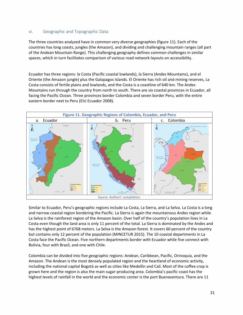
vi. Geographic and Topographic Data

The three countries analyzed have in common very diverse geographies (figure 11). Each of the countries has long coasts, jungles (the Amazon), and dividing and challenging mountain ranges (all part of the Andean Mountain Range). This challenging geography defines common challenges in similar spaces, which in turn facilitates comparison of various road network layouts on accessibility.

Ecuador has three regions: la Costa (Pacific coastal lowlands), la Sierra (Andes Mountains), and el Oriente (the Amazon jungle) plus the Galapagos Islands. El Oriente has rich oil and mining reserves, La Costa consists of fertile plains and lowlands, and the Costa is a coastline of 640 km. The Andes Mountains run through the country from north to south. There are six coastal provinces in Ecuador, all facing the Pacific Ocean. Three provinces border Colombia and seven border Peru, with the entire eastern border next to Peru (EIU Ecuador 2008).

Figure 11. Geographic Regions of Colombia, Ecuador, and Peru a. Ecuador b. Peru c. Colombia


Similar to Ecuador, Peru’s geographic regions include La Costa, La Sierra, and La Selva. La Costa is a long and narrow coastal region bordering the Pacific. La Sierra is again the mountainous Andes region while La Selva is the rainforest region of the Amazon basin. Over half of the country’s population lives in La Costa even though the land area is only 11 percent of the total. La Sierra is dominated by the Andes and has the highest point of 6768 meters. La Selva is the Amazon forest. It covers 60 percent of the country but contains only 12 percent of the population (MINCETUR 2015). The 10 coastal departments in La Costa face the Pacific Ocean. Five northern departments border with Ecuador while five connect with Bolivia, four with Brazil, and one with Chile. Colombia can be divided into five geographic regions: Andean, Caribbean, Pacific, Orinoquia, and the Amazon. The Andean is the most densely populated region and the heartland of economic activity, including the national capital Bogotá as well as cities like Medellín and Calí. Most of the coffee crop is grown here and the region is also the main sugar-producing area. Colombia’s pacific coast has the highest levels of rainfall in the world and the economic center is the port Buenaventura. There are 11

31

coastal departments in the Pacific and Andean regions. Three departments border with Ecuador, two with Peru, three with Brazil, and five with Venezuela (EIU Colombia 2008).

The study utilizes the Digital Elevation Model (DEM) and classifies the countries into 15 more granular geographies based on elevation and relief roughness, which is the maximum elevation minus the minimum elevation of a defined area divided by half the area length (Meybeck and Vörösmarty 2001). The results indicate that all three countries have very rough terrains, with 44 percent, 75 percent, and 74 percent of the land area being hilly or mountainous for Colombia, Ecuador, and Peru respectively (table 5).

Table 5. Terrain Classes and Percentage of Land Area in Colombia, Ecuador, and Peru

Class Description Colombia Ecuador Peru (% of total land)

1 Plains 0.64 0.06 0.11 2 Mid-altitude plains 0.00 0.00 0.00 3 High-altitude plains 0.00 0.00 0.00 4 Lowlands 15.99 5.11 10.92 5 Rugged lowlands 35.37 2.47 17.41 6 Platforms (very low plateaus) 2.93 0.00 1.48 7 Low plateaus 0.19 0.00 0.05 8 Mid-altitude plateaus 0.01 0.00 0.00 9 High plateaus 0.08 0.01 0.72 10 Very high plateaus 0.00 0.00 0.14 11 Hills 20.35 31.77 20.83 12 Low mountains 6.20 8.83 7.44 13 Mid-altitude mountains 9.25 13.45 10.37 14 High mountains 8.83 20.77 16.81 15 Very high mountains 0.15 1.39 13.70


Another key element to consider when analyzing accessibility, due to its significant impact on the design of road networks and planning of specific road link interventions, is the type of terrain. Needless to say, terrain characterization is also a key attribute to consider in an analysis of reliability (with or without weather-related shocks). In this study, terrain characteristics for each segment of the three road networks were derived using the GIS tool linear feature extraction. Linear feature extraction involves extracting elevation data at fixed intervals along the line of the road network and directly computing the road characteristics required for the topological categories to be used. Terrain classes were then calculated making assumptions about key road characteristics for each link: rise and fall, number of rises and falls, horizontal curvature, super-elevation, and altitude.14 Basic steps required for this approach are presented in figure 12.

14 An alternative method known as landscape classification was also were tested for this exercise. The linear feature extraction method turned out to represent road characteristics more accurately with slightly less stringent data assumptions. For details, see annex 3.

32

Figure 12. The Linear Feature Extraction Approach to Define Terrain Types

Source: World Bank based on GIS data.

Once the road characteristics are computed, each road segment is assigned to one of seven general classes of road geometry. For the purpose of this study, terrain class refers to seven different terrain or topological categories: straight and level, mostly straight and gently undulating, bendy and generally level, bendy and gently undulating, bendy and severely undulating, winding and gently undulating, and winding and severely undulating. vii. Economic Data

Many options were considered as the main source of economic data. A natural candidate—given the level of details in terms of economic sectors, labor, and capital needs—were the Enterprise Surveys. Enterprise surveys are firm-level surveys conducted by the World Bank since 2002. The surveys are mainly designed to assess the country’s business environment and obstacles to growth. The surveys have a geographic component and are representative at the region level. Geographic locations within a country are chosen based on the locations with the highest economic activity.15

For the three countries in the study, the surveys were conducted in 2006 and 2010. In Colombia, the sampled locations are four cities: Barranquilla, Bogotá, Calí, and Medellín. In Perú, firms in the cities of Arequipa, Lima, Chiclayo, and Trujillo were surveyed. Meanwhile, the enterprise surveys were conducted at the provincial level in Ecuador with the regions included being Azuay, Guayas, and Pichincha. However, Enterprise Surveys only consider firms located in the most economically concentrated places while foregoing the rest of the country where development is often in need of development.

To better understand the geographic disparities within a country, the study looked at two georeferenced dataset: nightlights derived from the Defense Meteorological Satellite Program/Operational Linescan System (DMSP/OLS) and a Global Reference Layer of Built-up Area.

Nightlights data have been used to asses urban expansion, capture the scope of human activity, and even proxy economic intensity (Lo 2002; Amaral and others 2006; Ghosh and others 2010). Nightlights are also used as a proxy of subnational economic activity. The DMSP/OLS nighttime stable light data

15 http://www.enterprisesurveys.org/methodology.

33

provide a potential way to map the extent and dynamics of urban areas. The DMSP flies in a sun-synchronous orbit, and the OLS (Operational Linescan System) is one of the main sensors on the DMSP satellite platform. At night, the OLS sensor can detect the lowest levels of radiation, hence, its nighttime light data are often used to study human activities, urban expansion, and economic activity. The nightlight dataset used in this analysis (2011) underwent a series of radiometric calibrations to address the saturation problem (that is, the lack of variation in the higher end) in urban centers. The radiance calibrated product is a relative measure and thus deemed to be unit-less (that is, a city which has a digital value of 400 in nightlights is not two times brighter than a city with a value of 200) (Feng-Chi 2015).

Nightlights data have been used as proxy for GDP, as presented in the seminal paper by Henderson and others (2012). The approach of Henderson and others (2012) to obtain measures of GDP growth builds on satellite imagery. Since 1992, a fleet of U.S. Air Force satellites has been collecting imagery of the Earth's surface every evening between 8:30 PM and 10:00 PM local time. These satellites are equipped with sensors to detect light reflectance and emissions, including lights emitted by man-made sources. After filtering out confounding sources of light, government scientists obtain a residual collection of reliable imagery which they combine to form one average image of the entire globe per year. Since the publication of Henderson and others (2012), lights data have become a popular predictor of income growth. By recovering parameters of the lights-GDP functional relationship from cross-country data, a researcher can apply these parameters to predict the lights-GDP relationship at subnational levels, where GDP estimates are often unreported.

Analysis of Nightlights dates makes evident the enormous concentration of economic activity in a few cities of the three countries studied. For Colombia, most economic activity is concentrated in the Andean and Caribbean coastal cities of Bogotá. For Ecuador, economic activities are concentrated in the coastal and mountainous cites, with Quito and Guayaquil having, by far, the largest economic intensity. Interestingly, when Ecuador is compared to Colombia, there is a fair amount of economic intensity in the Amazon (El Oriente), most likely due to the massive oil production of the region. Perú is unique in the sense that all activity is on the long and narrow coast, with Lima and Callao at the center.

34

Figure 13. Economic Intensity According to the Nightlights Datasets a. Colombia b. Ecuador c. Peru

Source: The Defense Meteorological Satellite Program/Operational Linescan System (DMSP/OLS).

The three countries’ economies are largely commodities driven. Therefore, it is important to identify the most productive regions in agriculture and mining. Data on the location of mining and reserves from InfoMine (2012/2013) and of agricultural production from the International Food Policy Research Institute’s (IFPRI’s) Spatial Production Allocation Model (2000) and the FAO’s Global Agro-Ecological Zones (GAEZ 3.0 for the year 2012) are also available.

According to data from InfoMine (figure 14), Colombia’s ongoing mining activities are concentrated in the northwestern part of the country. Gold, silver, and copper mining operations are mainly in the Andes Region and some coal production takes place in the departments of La Guajira and Cesar of the Caribbean Region. Ecuador has some gold, silver, and copper production in the southern part of the country but most of the potential mining sites are still being explored. Out of the three countries, Peru has the most mines (particularly gold, silver, copper, and zinc) distributed throughout La Sierra. Meanwhile, iron ore and tin are solely produced in the departments of Ica and Puno, respectively.

35

Figure 14. Mining Location a. Colombia b. Ecuador c. Peru

Source: InfoMine (2012/13).

The GAEZ agricultural productions maps can help identify the hotspots of agricultural production as shown in figure 15. The gradient color map depicts the total value in international dollars of all crops grown in the area. In Colombia, most of the agricultural production is in the Andes and Caribbean regions. Tolima, Magdalena, and Valle del Cauca are the top three departments in terms of total agricultural output. In contrast, the vast majority of the Amazon region has no agricultural production.

In Ecuador, agricultural production is predominately concentrated in the provinces of Guayas, Pichincha, and Esmeraldas. Peru, again, following the same pattern shown by nightlights and mining production, has high agricultural output along the coast and across La Sierra.

Figure 15. Total Agricultural Production a. Colombia b. Ecuador c. Peru

Source: FAO’s Global Agro-Ecological Zones (2012).

36

viii. Social Data

Harmonized household surveys are obtained from the Socio-Economic Database for Latin America (SEDLAC) through the LAC equity lab. The income variables are harmonized using PPP measures so that they are comparable across countries. The sample households also have a geographic component and for Colombia, Ecuador, and Peru the surveys are representative at the national level. The geographic regions used in the sampling procedure are defined by the country; income and welfare indicators can be computed at these subnational levels (table 6).

Table 6. Income and Welfare Indicators

Peru 2009

Monthly Income per Capita (PPP)

Population under $4 PPP

Access to Water

Access to toilet

Access to Electricity

Access to Telephone

Access to Internet

Car Ownership

$ per capita Percentage of total population Peru (2009)

Lima 456.56 7 88 92 99 92 23 17 Costa 269.37 20 79 77 92 81 8 9 Sierra 188.92 50 61 63 76 56 4 7 Selva 204.92 44 54 56 70 58 2 4

Ecuador (2010) Costa 238.61 34 87 92 97 27 7 13 Sierra 307.59 30 95 92 98 51 17 25

Amazonia 195.16 45 87 83 94 29 6 11 Colombia (2010)

Atlántico 205.90 49 84 85 92 81 12 7 Bogotá 522.85 13 99 100 100 98 34 20 Central 304.44 37 94 88 98 92 21 12 Oriente 278.67 32 89 92 98 90 13 13 Pacifico 229.68 44 87 84 96 85 13 9


The Lima metropolitan area and Bogotá are the wealthiest with the highest per capita income and lowest poverty rate (percent of the population under $4 PPP poverty line). In addition, despite the fact that the majority of the households have basic access to services (for example, water, toilet, and electricity), access to Internet and car ownership lag; 20 percent or less of the households in each region across the countries have access to Internet or cars except in Lima and Bogotá, where the figure is still only 23 percent and 34 percent, respectively.

One of the drawbacks of household surveys is that they say little about where people are. A spatial population model, Landscan (2012) which was developed by the Oak Ridge National Lab for the U.S. Department of Defense, uses a multivariable dasymetric approach to disaggregate census counts within an administrative boundary and provides global population distribution at 1 km resolution.16

16 http://web.ornl.gov/sci/landscan/.

37

As depicted in figure 16, the three countries are highly urbanized with a few places of very high population density. The case of Peru is the most striking. The Lima Metropolitan area is the only population center (dark red) in the country. The disaggregated population dataset is used in the study to generate an urban friction mask (box 5) and in the analysis of accessibility.

Figure 16. Population Distribution a. Colombia b. Ecuador c. Peru


ix. Natural Hazards

Data on the location and frequency of volcanos, floods, fires, hurricanes, and landslides, as well as a multihazard index (scaled from 1 to 5) are available from the Global Disaster Risk Platform. Monthly and annual precipitation data are also available. The LAC region is vulnerable to natural disasters of all types—earthquakes, volcanoes, storms, droughts, floods, landslides, and so on. Coupled with the infamous El Niño phenomenon, these disasters pose a serious threat to people’s lives and assets. The World Bank Natural Disasters hotspots study (Dilley and others 2005) reveals that seven LAC countries are ranked in the top 15 globally in terms of percentage of GDP in areas exposed to three or more hazards.

Several types of natural disasters have been considered, including tsunamis, earthquakes, and the multihazard index for diagnostics purposes. A global flood risk model (GFLORIS 2015) was eventually used to assess the exposure and resilience of the countries’ road networks. It is a raster dataset of layers of inundation depth of different return periods (5 years to 1,000 years) derived from a global hydrological model that is used to carry out simulations of daily river discharge and runoff.

Flood risk is investigated under the baseline climate (which uses historical meteorological data between 1960 and1990) and flood risk factoring in climate change simulated by Global Climate Models. A detailed methodology of the construction of the GFLORIS dataset can be found in Winsemius and others (2013).

38

Figure 17. Flood Extent and Severity (Depth, dm), 100-Year Return Period a. Colombia b. Ecuador c. Peru


Figure 17 illustrates the flooding events of the 100-year return period under the baseline climate. The most severe floods (depth>10 meters) in the three countries are predominately in the Amazon, as expected. In Colombia, the Caribbean region is also heavily flood, particularly the department of Bolívar and La Guajira. This reflects the fact that the valleys of the Magdalena and Cauca rivers and the eastern savannahs are prone to floods during the two main monsoon seasons.

In Ecuador, the Guayas river basin is also captured in the flood data (Figure 17). The basin and the land drained by its tributaries measures up to 35,000 square km. Three departments in Northeastern Peru also incur some heavy floods. In addition, 2–5 meter floods are observed in Lima and Junín, where they overlap the Carretera Central, known locally as “always flooded.”

E) Combining Engineering with Geography to Calculate Road User Costs

i. Teasing out the Power of GIS using Engineering Estimates: HDM-4

A starting point to estimate economic distances is to move away from Euclidean distances into network distance and, ultimately, into cost, speed, and time distances as perceived by the user. It is in this context that the GIS analysis is combined with the more traditional engineering approach of estimation of user operating costs. For the study, the Highway Development and Management Model (HDM-4) provides estimates for two key metrics: road users costs (RUCs) and (vehicle) speed. RUCs are defined as the unit cost of using a road expressed in dollars per ton-kilometer. The road user costs (RUCs) consist of two components: vehicle operating costs (VOCs), which reflect the cost of operating a vehicle, and value of time costs

39

(VOTs), which reflect the cost of time associated with using a vehicle.17 HDM-4 also calculates the predicted vehicle speed in kilometers per hour for a given road link. HDM-4 uses two categories of inputs: data related to road characteristics and data related to vehicle fleets. Road characteristics are defined at the link level and vehicle fleet data are compiled at the national level. For the purposes of the study, the vehicle fleet data were collected at the country level with a heavy truck taken as the representative vehicle. Road characteristics are defined multidimensionally and for each potential link of a country network. The six characteristics are: • Network type: primary, secondary,

or tertiary • Terrain type: mostly straight and

level, mostly straight and gently undulating, bendy and generally level, bendy and gently undulating, bendy and severely undulating, winding and gently undulating, and winding and severely undulating

• Surface type: paved or unpaved • Pavement condition: good, fair, or

poor • Traffic class: expressed in annual

average daily traffic (AADT) (vehicles/day), <300, 300–1,000, 1,000–3,000, 3,000–6,000, 6,000–10,000, and > 10,000

• Number of lanes: one, two, four, or six (used to make assumptions about speed-flow type, which reflects vehicle flows based on road capacity) 18

Using these six characteristics (country and the country-specific vehicle fleet data associated with it amounts to a seventh characteristic), HDM-4 was used to calculate 6,804 road user costs and

17 The VOCs include the cost of fuel, lubricants, tires, maintenance parts and maintenance labor, crew time, depreciation, interest, and overhead. The VOTs include the cost of passenger time and the cost of cargo time. Each of these components is calculated separately as an output of the HDM-4 model. 18 A limited number of characteristics relevant to the three case studies were chosen. However, HDM-4 is quite flexible and allows for further calibration to include not only more characteristics but also more categories within each characteristic. For a more detailed description of the potential model inputs see HDM-4 Road Use Costs Model Documentation and Archondo-Callao (2008) and references therein.

Box 4. What the 6804 Road User Tell Us

The baseline set of 6,804 link types which are associated with each combination of attributes (characteristics and categories) can provide a sense of how each characteristic individually impacts road user costs.

Averaging all of the potential combinations for each country—without considering the actual length of the road network—indicates that road user costs tend to be highest in Peru at $1.70 per vehicle-km and lowest in Ecuador at $1.25 per vehicle-km. The difference is driven mainly by the price of oil, which is significantly subsidized in Ecuador.

In contrast, speed does not vary across countries. That is, speed varies across road characteristics but not across vehicle fleet characteristics. The mean speed for each country is 51.92 km/hour and the median is 46.08 km/hour.

The main drivers of user costs, as well as speed, are network (primary/secondary/tertiary), surface type (paved/unpaved), and road condition (good/fair/poor), in that order. Sensibly, average user costs are lowest on primary networks and highest on tertiary networks. Using unpaved roads tends to be at least 50 cents more costly than paved costs. Costs significantly increase as road condition declines.

The terrain type does not have a large impact on costs and speed except for the winding and severely undulating category

Interestingly, traffic shows negligible impact on user costs, perhaps due to HDM-4 not factoring in congestion. For additional details, see annex 4.


40

their components. This corresponds to all possible combinations of the three countries, the three network types, the seven terrain classes, the two surface types, the three pavement condition classes, the six traffic classes, and the three lane classes.19 Finally, to incorporate the impact of congestion, road user costs were recalculated for links in urban areas using speeds derived from Google Directions (box 5).

Box 5. Accounting for Urban Friction Due to higher traffic, urban centers tend to suffer from congestion problems (this is referred to as higher friction in the urban center in GIS terms). The average speeds of vehicles in the city are expected to be lower than in intercity corridors and even rural areas assuming all other conditions are equal. HDM-4 can be used to model congestion effects by inputting a reduced speed based on travel time and speeds calculated using Google’s Directions Application Program Interface ( API), which takes congestion into account. First, urban areas must be defined. This is done based on three criteria: percentage of built-up land; population; and status as a national or provincial capital. Roads which intersect the urban cluster mask are identified and considered “urban” for the purposes of analyzing urban friction. Travel time and speeds are then calculated for these roads using Google’s Directions API. An “urban friction coefficient” can be defined to provide a sense of congestion effects:

𝑈𝑈𝑚𝑚𝑎𝑎𝑎𝑎𝑜𝑜 𝐹𝐹𝑚𝑚𝑖𝑖𝑎𝑎𝑎𝑎𝑖𝑖𝑡𝑡𝑜𝑜 𝐶𝐶𝑡𝑡𝑎𝑎𝑖𝑖𝑖𝑖𝑖𝑖𝑎𝑎𝑖𝑖𝑎𝑎𝑜𝑜𝑎𝑎𝑖𝑖 = 1 − 𝐺𝐺𝑡𝑡𝑡𝑡𝑔𝑔𝑎𝑎𝑎𝑎 𝑆𝑆𝑜𝑜𝑎𝑎𝑎𝑎𝑚𝑚𝑖𝑖𝑖𝑖

𝑂𝑂𝑚𝑚𝑖𝑖𝑔𝑔𝑖𝑖𝑜𝑜𝑎𝑎𝑎𝑎 𝐻𝐻𝐷𝐷𝐻𝐻4 𝑆𝑆𝑜𝑜𝑎𝑎𝑎𝑎𝑚𝑚𝑖𝑖𝑖𝑖

The urban friction coefficient can be interpreted as the percentage speed reduction of the original HDM-4 speed estimates. For the urban road links in Colombia, Ecuador, and Peru, the average friction coefficients are 0.50, 0.36, and 0.39 respectively. In other words, there is on average a 50 percent speed reduction in Colombia, 36 percent speed reduction in Ecuador, and 39 percent speed reduction in Peru in the urban centers defined by the study. For the calculation of road user costs in HDM-4, the speeds derived from Google were inputted directly to the model and calculated as an additional road characteristic for all urban roads. That is, in the case of urban roads, HDM-4 was used to calculate the road user cost associated with an existing road link rather than the road user costs associated with a type of road based on the seven road characteristics. Source: Authors’ compilation. Note: For details see annex 5. ii. Characterizing the Road Networks

Each link in the geo-referenced road networks of the three countries is uniquely characterized by a single combination of seven attributes (country, network class, terrain type, surface type, condition type, traffic level, and number of lanes). The same is true for each estimation of road user cost (and speed) produced using HDM-4. It is the link provided by Thus, it is this vector of seven attributes which permits association between each road link and its associated road user costs. Ultimately, this is the “glue” which allows for the assessment of the importance of individual links in the total network, the estimation of accessibility indexes associated to specific road networks and, depending on the research or policy question, the impact of an investment project or other type of intervention on the road network.

19 Three countries * 3 network classes * 7 terrain types * 2 surface types * 3 condition types * 6 traffic levels * 3 lane types creates 6,804 combinations of road characteristics.

41

The resulting distribution of the total road networks into the topological classes by country indicates that between 53 and 67 percent of the total network under consideration is built on terrain challenging for construction (Table 7). The terrain composition translates into higher road and vehicle operating costs, greater economic distances in general, and higher investment and rehabilitation costs.

Table 7. More than Half of the Total Network is Built on Challenging Terrain (distribution of the total road network by terrain class)

Road Geometry Class Colombia

% Ecuador

% Peru

%

Straight and level 0 2 1 Mostly straight and gently undulating 43 34 15

Bendy and generally level 0 0 0 Bendy and gently undulating 5 8 17

Bendy and severely undulating 40 47 13 Winding and gently undulating 1 1 10

Winding and severely undulating 11 7 44

Source: World Bank based on GIS data. Note: For Colombia, only 11 percent of the secondary and 44 percent of the tertiary road network is included.

Ecuador has the flattest and straightest terrain while Peru and Colombia have much less even terrain. In all three countries, most traffic is less than 300 AADT (figure 18), and most roads have two lanes (figure 19). Figure 18. Most Traffic is Less than 300 AADT . . .

(percent of total road length by traffic level) Figure 19. . . . and Most Roads Have Two Lanes

(percent of total road length by number of lanes)

Source: World Bank based on HDM-4 and GIS data. Source: World Bank based on HDM-4 and GIS data.

Turning to road user costs, distance-weighted RUCs can provide a sense for average road user costs across the existing networks in Colombia, Ecuador, and Peru. Distance-weighted mean RUCs are highest in Peru ($1.95 per vehicle-km), followed closely by Colombia ($1.91 per vehicle-km). They are substantially lower in Ecuador at $1.48 per vehicle-km. In contrast, distance-weighted average speed is slightly higher in Peru at 44 km/hour while it is 39 km/hour in both Colombia and Ecuador.

0%10%20%30%40%50%60%70%80%90%

100%

Traffic Level


0%10%20%30%40%50%60%70%80%90%

100%

2 lanes 4 lanes 6 lanes

Number of Lanes


42

Figure 20. Distance-weighted Costs are Highest

in Peru and Lowest in Ecuador (average RUCs ($/vehicle-km))

Figure 21. Average Speed is Slightly Higher in Peru than in Colombia and Ecuador

(average speed (km/hour))


Average RUCs are much lower on primary than secondary roads in Colombia (Figure 22).The difference is less striking in the other two countries ($0.67 per vehicle-km in Colombia versus $0.39 and $0.32 per vehicle-km in Ecuador and Peru, respectively). In Colombia and Ecuador, the difference in average RUCs on secondary and tertiary networks is not very large ($0.14 and $0.13 per vehicle-km, respectively), while in Peru, the difference is quite substantial ($0.43 per vehicle-km). Consistent with these findings about average cost, average speed is significantly higher on Colombian primary roads (32 km/hour faster than on secondary roads) while speeds are significantly lower on tertiary than secondary roads in Peru (14 km/hour lower) but not in Colombia and Ecuador (figure 23).

Figure 22. RUCs are Much Lower on Primary

than Secondary Roads in Colombia (average RUCs [$/vehicle-km] by network type)

Figure 23. Average Speed is Much Higher on the Primary Network in Colombia

(average speed [km/hour] by network type)


Distance-weighted average cost generally increases and speed generally decreases as terrain becomes more variable, though there is substantially less variation in both in Ecuador than in Colombia and Peru (figure 24). The largest increase in cost is $0.69 per vehicle-km in Colombia between straight and level and mostly straight and gently undulating terrain. The difference between these terrain types is also substantial in Peru ($0.36 per vehicle-km). The largest decrease in speed is also in Colombia moving from straight and level to mostly straight and gently undulating terrain: speed declines 30 km/hour (the difference between these terrain types is 20 km/hour in Peru) (figure 25).

$1.91

$1.48

$1.95

$-

$0.50

$1.00

$1.50

$2.00

$2.50


RUCs

($/v

ehic

le-k

m) 39 39

44

0

10

20

30

40

50


Spee

d (k

m/h

our)

$1.29

$1.96 $2.10

$1.15 $1.54 $1.67

$1.39 $1.72

$2.15

$-

$0.50

$1.00

$1.50

$2.00

$2.50

Prim

ary

Seco

ndar

y

Tert

iary

Prim

ary

Seco

ndar

y

Tert

iary

Prim

ary

Seco

ndar

y

Tert

iary


RUCs

($/v

ehic

le-k

m)

Overall Average

66

34 31

55

34 30

67

51 36

01020304050607080

Prim

ary

Seco

ndar

y

Tert

iary

Prim

ary

Seco

ndar

y

Tert

iary

Prim

ary

Seco

ndar

y

Tert

iary


Spee

d (k

m/h

our)

Overall Average

43

Figure 24. Distance-weighted Costs Generally Increase as Terrain Becomes More Variable.

(average RUCs ($/vehicle-km) by terrain type)

Source: World Bank based on HDM-4 and GIS data.

Figure 25. . . .and Speeds Generally Decrease (average speed (km/hour) by terrain type)


$-

$0.50

$1.00

$1.50

$2.00

$2.50

Straightand level

Mostlystraight and

gentlyundulating

Bendy andgenerally

level

Bendy andgently

undulating

Bendy andseverely

undulating

Windingand gentlyundulating

Windingand

severelyundulating

Colombia Ecuador Peru Overall Average

0

10

20

30

40

50

60

70

80

Straight andlevel

Mostlystraight and

gentlyundulating

Bendy andgenerally

level

Bendy andgently

undulating

Bendy andseverely

undulating

Winding andgently

undulating

Winding andseverely

undulating


44

Figure 26. RUCs and Speeds Generally Behave as Expected Across Surface Type, Road Condition, Traffic Level, and Number of Lanes

(average RUCs [$/vehicle-km] and average speeds [km/hour] by surface type, road condition, traffic level, and number of lanes)

a. Road Surface: RUCs

b. Road Surface: Speed

c. Road Condition: RUCs

d. Road Condition: Speed

e. Traffic Level: RUCs

f. Traffic Level: Speed

g. Number of Lanes: RUCs

h. Number of Lanes: Speed


Note: RUC = road users costs.

$1.15

$2.06

$0.84

$1.56 $1.38

$2.34

$- $0.50 $1.00 $1.50 $2.00 $2.50

Pave

d

Unp

aved

Pave

d

Unp

aved

Pave

d

Unp

aved


73

32

73

35

65

29

01020304050607080

Paved Unpaved Paved Unpaved Paved Unpaved


$1.18

$2.05 $1.71

$1.01

$1.56 $1.65 $1.34

$1.88 $2.38

$-

$0.50

$1.00

$1.50

$2.00

$2.50

Good Fair Poor Good Fair Poor Good Fair Poor


Overall Average

71

33 46

64 35

32

66

45 29

0

20

40

60

80



Overall Average

$- $0.50 $1.00 $1.50 $2.00 $2.50

<300

300-

1,00

0

1,00

0-3,

000

3,00

0-6,

000

6,00

0-10

,000

<300

300-

1,00

0

1,00

0-3,

000

3,00

0-6,

000

6,00

0-10

,000

<300

300-

1,00

0

1,00

0-3,

000

3,00

0-6,

000

6,00

0-10

,000


Overall Average

32

53 62

72 67

34

56 55 59 65

40

66 73 66 76

0102030405060708090

<300

300-

1,00

0

1,00

0-3,

000

3,00

0-6,

000

6,00

0-10

,000

<300

300-

1,00

0

1,00

0-3,

000

3,00

0-6,

000

6,00

0-10

,000

<300

300-

1,00

0

1,00

0-3,

000

3,00

0-6,

000

6,00

0-10

,000


Overall Average

$2.09

$1.29

$-

$1.49 $1.02

$1.07

$2.06 $1.49

$1.26

$-

$0.50

$1.00

$1.50

$2.00

$2.50

2 lanes 4 lanes 6 lanes 2 lanes 4 lanes 6 lanes 2 lanes 4 lanes 6 lanes


Overall Average

31

66

38

61

51

39

61

75

0

10

20

30

40

50

60

70

80

2 lanes 4 lanes 6 lanes 2 lanes 4 lanes 6 lanes 2 lanes 4 lanes 6 lanes


Overall Average

45

Road user costs generally increase and speeds generally decrease from paved to unpaved roads, with deterioration in road condition, and as the number of lanes declines (figure 26). However, there are several exceptions. In Colombia, average RUCs are actually lower on roads in poor condition than they are on roads in fair condition; similarly, speeds are higher on roads in poor condition than they are on roads in fair condition in Colombia. In Ecuador, there is a decline of 10 km/hour from four-lane roads to six-lane roads. Interestingly, as traffic levels increase costs generally decline. This is likely because more-traveled roads are also paved primary roads in better condition, which are more important cost drivers than traffic levels.

Road user costs are dominated by fuel costs in Colombia and Peru, where they make up more than 40 percent of total cost (41 and 48 percent, respectively) (table 8). The parts components of maintenance also has a substantial impact, representing around 30 percent of total cost in both countries. Depreciation is the third-largest driver of costs in the two countries. The composition of total cost is different in Ecuador, where fuel subsidies mean that only 13 percent of total cost is made up of fuel costs. The parts component of maintenance drives most of total cost (41 percent) while depreciation, crew, and the labor component of maintenance all compose 10 to 15 percent of total road user cost. Value of time costs are negligible.

Table 8. RUCs are Dominated by Fuel Costs in Colombia and Peru but Not in Ecuador (percent of total RUCs by cost component)

Cost Component Colombia %

Ecuador %

Peru %

Vehicle Operating Costs

Fuel 41 13 48 Lubricants 1 1 2

Tires 3 2 4 Maintenance: Parts 31 41 30 Maintenance: Labor 5 11 3

Crew 5 12 3 Depreciation 9 14 7

Interest 4 5 3 Overhead 0 0 0

Value of Time Costs Passenger time 0 0 0

Cargo time 0 0 0

Source: World Bank based on HDM-4 and GIS data. Note: RUC = road users costs.

A simple, country-specific OLS regression was run with road user costs as the output variable and road characteristics as the inputs (annex 4). The road characteristic with the largest impact on RUCs is unpaved roads: moving from a paved to an unpaved road increases RUCs more than $0.40 per vehicle-km in Colombia and Ecuador and $0.79 in Peru. Network class (less so in Peru), condition, and winding and severely undulating terrain type all lead to substantially increased road user costs in each of the three countries. The story is similar for speed: network class, condition, and, particularly, surface type are particularly important determinants of speed (annex 4). A winding and severely undulating terrain type also results in substantially decreased speeds.

46

II. PART 2: Spatial Disparities through the Accessibility Lens

Accessibility estimates are expressed in tons/$, or alternatively vehicles/$. This means in practice that, broadly speaking, accessibility estimates can be interpreted as the potential economic activity (or opportunities for human or economic interaction) unlocked by a specific transport network connecting origins with destinations. In other words, the accessibility indicator quantifies the degree of opportunities for interactions between two or more specific locations given the cost borne by the user to “move” from one location to another. The higher its level the higher the accessibility and with that the better the opportunities for interaction (human or economic exchanges) between locations, namely cities, ports, airports, or simply areas of interest. Measures of accessibility are always defined over a predetermined physical space. In this section, the analysis begins by presenting accessibility indicators for each country separately with country borders defining the universe of origins and destinations.20 With this set of results, the section addresses the question of how different definitions of accessibility characterize the efficiency of a road network with respect to facilitating (or unlocking) social and economic opportunities for

20 This is as opposed to a multicountry or regional accessibility specification.

Box 6. Narrowing Down to a Sensible Accessibility Indicator

In the process of defining and selecting options for accessibility estimates, many alternatives were explored using different functional forms for the impedance or friction component of the formula as well as different weights. The two functional forms selected are the inverse cost—to model the infrastructure-based accessibility—and the population-weighted gravity indicators—to model the location-based accessibility.

While there are significant differences in the level and distribution of the infrastructure-based accessibility and the group of all location-based accessibility estimates, all location-based measures estimated seem highly correlated among themselves, and can even be used interchangeably. Perhaps what they reflect is that essentially only two weights have been tried—population and gross domestic product (GDP)—and the proxy for GDP is the Nightlights index. The Nightlights index comes with imperfections. One of the most salient criticisms is that it could be a good proxy of economic activity in highly industrialized countries and at some level of urbanization. In all other cases, the Nightlights might be reflecting population density and not necessarily economic intensity. This introduces a lot of noise as a proxy for GDP for countries with economies driven by low-labor industries, namely mining or commodity economies. That is the case of Colombia, Peru, and Ecuador (and in fact of most Latin America). A more structural problem is that Nightlights is a relative rather than absolute measure, therefore its use to limited when trying to compare accessibility indexes and normalize then in there of share of contribution of a node to the total GDP.

The correlation of the population-based and the Nightlight-based accessibility estimates is evident in the results for Colombia, Peru, and Ecuador when taking a look to the disaggregated (by node) results. Unfortunately at the time of preparing this report, no other measure of GDP at a local level was available for all countries. Given that limitation, for the purpose of the accessibility analysis presented in this report, only estimates using population weights are considered. The data used for population are very reliable, and with great confidence, comparable and standardized across countries.

The second decision pertains to the functional forms to use, even if only using population weights for the location-based accessibility estimates. Given the enormous correlation between all of them, for practical purposes and to make sure the accessibility indicators have easy interpretation and replicability, the study focuses on the simplest form: gravity with population weights. Source: Authors’ compilation. Note: For details see annex 8

47

interaction. This will be done by comparing the characterization of the accessibility of Colombia, Peru, and Ecuador using infrastructure-based accessibility and location-based accessibility. Next, the report uses the detailed results of the population-weighted gravity accessibility indicators (location-based) to understand how accessibility is challenged by geography, terrain, and subregional wealth. Finally, we try to start the debate of how accessibility measures could help identify the challenges and successes of the existing road network. This is done from two perspectives. The first perspective is strictly social, estimating accessibility in a predetermined fixed catchment area or buffer around each node. A 100 kilometer (km) ratio is defined—admittedly arbitrarily—to compare changes in accessibility when controlling for distance. The second perspective is to define accessibility with respect to access to markets (cities) and to the services which help goods reach markets (ports, airports, and border crossings).

As described in the introductory sections of the report, accessibility can be measured in many different ways with important variations even within the infrastructure-based and location-based measures employed here. The following sections emphasize accessibility as it relates to opportunities, beginning with a baseline measure which excludes those opportunities and moving on to a weighted measure which incorporates them. Annex 8 provides a detailed description of each measure, along with alternative specifications including the use of local economic activity weights, an empirically estimated impedance function, and competition weights which might be more appropriate for different types of accessibility analyses.

A) Characterizing Accessibility: Engineers and Economists Working Together

The infrastructure-based approach provides a baseline measure for assessing accessibility. This analysis measures an origin’s connectivity to the most economically and socially important destinations in Colombia, Ecuador, and Peru. Though access to faraway borders, ports, airports, and cities may not provide a very practical measure of mobility, it does provide a general picture of the places which are easy and not-so-easy to reach (and depart from).

The measure considers only the cost of traveling between an origin and destination. These origins and destinations are all cities with populations over 25,000, border crossings, ports, and airports. The accessibility of an origin to itself (“self-potential”) is not considered. However, when any of the noncity nodes is fewer than 20 km apart as the crow flies, they are considered to be a single node. This results in 137 nodes in Colombia, 51 in Ecuador, and 93 in Peru. The infrastructure-based approach is calculated as the sum of the inverse of the accumulated transport costs on the least-cost route between each origin i and each destination j. The inverse functional form recognizes the theoretical proposition that accessibility should decrease as costs increase.

𝐴𝐴𝑖𝑖 = � �1

𝑜𝑜 − 1� ∗ 𝑖𝑖(𝑎𝑎𝑖𝑖𝑗𝑗)

𝑛𝑛

𝑗𝑗=1;𝑗𝑗≠𝑖𝑖

= ��1

𝑜𝑜 − 1� ∗ �

1𝑎𝑎𝑖𝑖𝑗𝑗)�

𝑛𝑛

𝑗𝑗=1

The sum of the accumulated inverse costs of traveling between each origin and destination is weighted by the number of destinations (the origin is excluded as a destination so there are n-1 destinations). Costs are multiplied by 25 to convert $/vehicle into $/ton and accessibility is expressed as tons per $100.

Average accessibility is highest in Ecuador at 10.36 t/$100, nearly twice as high as Colombia’s 5.65 t/$100 and three times Peru’s 3.37 ton/$100 (table 9). This implies that more goods can be transported

48

for a dollar in Ecuador than in Colombia and Peru, which is consistent with both Ecuador’s smaller size and the lower average road users costs (RUCs)—driven by subsidized fuel—in Ecuador. Ecuador also has the origin with the highest accessibility, Atuntaquí in Ecuador’s Sierra region in the country’s north. Armenia in the Andina region of Colombia to the west of Bogotá has that country’s highest accessibility while Peralvillo in the center of Peru’s Costa region is the highest in that country. Ecuador’s most accessible origins are in the Sierra and Costa regions, while Peru’s most accessible are all in the Costa region. Colombia’s, in contrast, are in the central Andina region of the country. Interestingly, Ecuador’s population centers—Guayaquil and Quito—and Peru’s—Lima—appear among the top five most accessible origins in each country, while only Colombia’s tenth-most populous city makes the top five in that country (Bogotá ranks 17th). All of the most accessible origins are cities.

Table 9. Accessibility is Highest in Ecuador and Lowest in Peru on the Infrastructure-based Accessibility Measure (ton/$100)

Colombia Ecuador Peru Mean 5.6 10.3586 3.37

SD 1.9 3.3 1.6 Max Name Armenia Atuntaqui Peralvillo Max Score 10.3 16.4 8.4 Min Name Puerto Carreño Pte de Integración Iquitos Min Score 1.2 3.5 0.9

Source: Authors’ compilation. Note: SD is standard deviation.

The Peruvian Amazonian city of Iquitos, isolated in the northwest of the country, is the least accessible origin in the three countries, followed by Puerto Carreño, a city in the northwestern tip of Colombia surrounded by Venezuela, and by Puente de Integración in Ecuador, a border crossing with Peru in the south. The range of scores is highest in Ecuador and lowest in Peru. Four of the five least accessible cities in Ecuador are in the Oriente region, similar to Peru where all five are in the Selva region. Again, the geography of accessibility in Colombia is somewhat different with the least accessible cities in three different regions (Amazónica, Caribe, and Orinoquía) and ranging from La Macarena Airport in the south-central portion of the country to Puerto Carreño in the northwest. The least accessible origins are a mix of airports, cities, and border crossings. No ports are among the least accessible.

While the infrastructure-based measure provides a rough sketch of accessibility, it does not capture the opportunities which motivate travel. Incorporating the population of each node into the measure of accessibility in a “location-based” measure can provide a more accurate depiction of accessibility because it reveals how well people at different origins are able to access the centers of population which drive most economic and social activity. As described in the introduction, the ability of roads to transport people matters but it is the ability of roads to transport people to places of opportunity which is critical for development. In this case, accessibility is again measured as the sum of the accumulated inverse costs of traveling between each origin and destination. However, these costs are now weighted by the share of the total population of origin i's destinations, representing the opportunities for interaction available at those destinations. While economic activity – for instance, local “GDPs” – might be a superior measure of opportunities, such data is hard to come by and the data which is available exhibits a high correlation with the population weight (annex 8 for a detailed description of the

49

application of one measure of local economic activity, nightlights, to the accessibility analysis.). Again, origin i is not included as a destination and so its population is excluded.

𝐴𝐴𝑖𝑖 = �𝑃𝑃𝑡𝑡𝑜𝑜𝑆𝑆ℎ𝑎𝑎𝑚𝑚𝑎𝑎𝑗𝑗 ∙ 𝑖𝑖�𝑎𝑎𝑖𝑖𝑗𝑗�𝑛𝑛

𝑗𝑗=1

= �𝑃𝑃𝑡𝑡𝑜𝑜𝑆𝑆ℎ𝑎𝑎𝑚𝑚𝑎𝑎𝑗𝑗 ∙ �1𝑎𝑎𝑖𝑖𝑗𝑗�

𝑛𝑛

𝑗𝑗=1

The effect of adding the population weight is revealing. First, mean scores are similar between the population measure and the infrastructure-based measure, suggesting that accessibility overall is similar between the measures (their correlation is 0.72). However, the maximum accessibilities are significantly higher in the location-based measure, reflecting the uneven distribution of population across origins. (table 10). As figure 27 shows, the distribution of the two measures is largely similar, though the location-based measure has a long tail of origins with very high accessibility. Notably, the location-based measure does not result in extremely low accessibility measures.

Table 10. The Mean of the Infrastructure- and Location-based Measures are Similar but the Maximum Values are Much Higher Using the Location-based Measure (Tons/$100)


SD 4.0 8.2 6.1 Max Name La Pincha Alfaro Chaclacayo Max Score 34.8 51.8 34.2 Min Name Puerto Carreño Pte De Integración Iquitos Min Score 1.3 3.4 0.8

Source: Authors’ compilation. Note: SD is standard deviation.

50

Figure 27. The Distribution of the Two Accessibility Measures is Similar, but the Location-based Measure Has a Long Right Tail


The high-accessibility origins uncovered by the location-based measure suggest that the failure of the infrastructure-based measure to consider the opportunities unlocked by travel is meaningful: these origins capture the substantial concentration of the populations—and opportunities—of Colombia, Ecuador, and Peru in several cities and so the increased potential of places which can reach these locations at lower cost. As centers of population, these cities are the drivers of opportunities, which the accessibility measure reflects. Figure 28 provides a similar picture to figure 27, but emphasizes that there are about equal gains and losses in accessibility when the population weight is added for the majority of cities but substantial gains in accessibility for several.

0.1

.2.3

.4D

ensi

ty

0 10 20 30 40

Infrastructure-Based Location-Based

Colombia

0.2

.4.6

Den

sity

0 10 20 30 40 50


Ecuador

0.1

.2.3

.4.5

Den

sity

0 10 20 30 40


Peru

51

Figure 28. Several Origins have Much Higher Accessibility on the Location-based Measure Than on the Infrastructure-based Measure


The top five most accessible cities are also different in most cases from the top five most accessible cities in the infrastructure-based measure, suggesting that the location-based measure does not simply accentuate the accessibility of certain origins but provides unique information about how easily goods can reach important markets.

Sensibly, the cities with the largest accessibilities in the location-based measure are places which are close to large cities, rather than the large cities themselves. The case of Lima is instructive. The importance of Lima in Peru is underscored by the location-based measure, in which all of the five most accessible origins are less than 50 km from Lima as the crow flies. The situation is the same in Ecuador where the five most accessible origins are less than 51 km from Guayaquil and Quito and in Colombia where the most accessible origins are less than 50 km from Bogotá in four cases and from Medellín in one.

Figure 29 shows the accessibility of Colombia, Ecuador, and Peru with darker red indicating less accessible areas and darker green indicating more accessible areas. Each country is mapped using the same color gradient to make cross-country comparison possible. It is important to note, however, that the different land areas of each of these countries impacts their accessibility scores. Ecuador’s territory is one-fourth of the size of Colombia’s and one fifth the size of Peru’s, which is reflected in its much higher accessibility (the green in figure 29). This characteristic of the accessibility measure has both desirable and undesirable characteristics. On the negative side, when countries vary greatly in size the measure will reflect these differences in size in differences in accessibility. On the positive side, the measure is serious about theory in emphasizing that origins and destinations which are farther apart require more costly travel.21 That said, once analyzing accessibility scores within a single country (which essentially controls for land area), it is the variation in accessibility which is important: the greenest areas in Ecuador are the most accessible, while the yellow ones are very inaccessible. The accessibility measure’s future usefulness can be enhanced by performing the analysis in more countries to facilitate benchmarking and by re-running the analysis at the regional level to understand the full scope of interactions among and between origins and destinations.

21 Future research should explore intraregional analysis which would overcome this problem.

05

1015

20In

frast

ruct

ure-

Bas

ed

0 10 20 30 40 50Location-Based

Colombia Ecuador Peru Line of Equality

Location-Based vs. Infrastructure-Based

52

Turning to such an intracountry analysis, dark green covers a wide swatch of the western portion of Ecuador with Guayaquil and Quito exerting a powerful effect on origins in this area. Areas of lowest accessibility in Ecuador are indicated by the yellow and yellow-green colors in Sucumbíos in the north and Loja and Zamora Chinchipe in the south.

The map of Colombia’s accessibility shows more diversity than that of Ecuador. Only the very center of the country surrounding Bogotá has dark green indicating high accessibility. Accessibility largely declines with distance from Bogotá, increasing around Medellín and Cali, Colombia’s second- and third-largest cities. Cartagena is a bright spot of higher accessibility on the Atlantic coast.

Much of Peru’s territory is dominated by orange and red indicating very low accessibility. This is especially true in the northeastern part of the country surrounding Iquitos and in the southeastern portion bordering Brazil and Bolivia. There are two bright spots: Lima on the central coast and Chiclayo on the northern coast. Unlike in Ecuador where Guayaquil and Quito created larges areas of accessibility and even in Colombia where Bogotá, Medellín, and Cali did the same, in Peru Lima and Chiclayo’s sphere of influence is quite limited.

Figure 30, which graphs the distance from each origin to each country’s largest city, emphasizes this effect: Lima’s influence on accessibility declines much more quickly as distance increases while in Ecuador and Peru the largest city continues to exert influence (see especially Ecuador’s origins at around 400 km) even as distance increases. Lima is truly critical to accessibility in Peru.

Figure 29. Location-based Accessibility a. Colombia B. Ecuador c. Peru


53

Figure 30. Accessibility Declines More Quickly with Distance from Lima Than from Bogotá and Guayaquil


B) Challenges for Achieving Good Accessibility

i. Geography and Accessibility

Figure 31 shows the regional breakdown of location-based accessibility in the three countries. Some clear messages begin to emerge. In Peru and Ecuador, accessibility is highest in the Costa regions (and in the Sierra in Ecuador) while in Colombia accessibility is higher in the central Andina region (figure 32). The eastern parts of the countries—farthest from the coast and primarily in the Amazon—have the lowest accessibility. Interestingly, the terrain type of the origin city does not seem to have a strong relationship to the level of accessibility (figure 33). Ecuador and Peru are again set apart somewhat from Colombia: the former countries have the highest levels of accessibility on plains whereas Colombia’s accessibility is highest on plateaus. Somewhat counterintuitively, Colombia’s second-highest accessibility is in mountainous areas and Colombia and Ecuador’s lowest accessibility is in lowlands.

010

2030

4050

Loca

tion-

Bas

ed A

cces

sibi

lity

(tons

/$10

0)

0 500 1000 1500 2000Distance from largest city (km)


Accessibility vs. Distance

54

Figure 31. Accessibility is Highest in the Costa Regions in Ecuador and Peru and in the Andina Region of Colombia

(Mean location-based accessibility by subregion, tons/$100)


Figure 32. Location-based Accessibility by Region

a. Colombia B. Ecuador c. Peru


8.0 6.5

4.7 4.4 3.5 2.9

15.2 13.6

12.8

5.8 7.3

4.7 2.9 2.2

0.02.04.06.08.0

10.012.014.016.0

And

ina

(81)

Col

ombi

a (1

33)

Pací

fica

(3)

Car

ibe

(37)

Am

azón

ica

(6)

Ori

noqu

ía (6

)

Cos

ta (1

9)

Sier

ra (2

0)

Ecu

ador

(48)

Ori

ente

(9)

Cos

ta (4

0)

Peru

(90)

Sier

ra (2

9)

Selv

a (2

0)


55

Figure 33. Terrain Type Does Not Have a Consistent Relationship to Accessibility across Countries (Mean location-based accessibility by terrain type, ton/$100)


ii. Population and Accessibility

The relationship between population and accessibility is mixed. In Colombia and Ecuador, there seems to be a tendency for medium-sized origins to have higher accessibilities (Table 11). This suggests that smaller origins are less connected and that very large origins have fewer external opportunities. However, the largest city in Colombia and the largest cities in Ecuador both have relatively high accessibility scores. .There is no clear pattern in Peru, though origins with 100,000 to 250,000 people have higher accessibility than those with 50,000 to 100,000 people and those with 250,000 to 500,000 people.

Table 11. Accessibility is Lowest in the Smallest and Largest Cities in Colombia and Ecuador (Location-based accessibility by origin population, ton/$100)

Colombia Ecuador Peru Origin Population Score # Score # Score #

0 to 50,000 5.9 71 11.3 20 5.9 29 50,000 to 100,000 7.2 23 12.5 8 3.4 26

100,000 to 250,000 8.5 20 15.5 14 5.5 15 250,000 to 500,000 5.6 10 11.0 4 3.1 15 500,000 to 1 million 5.1 5 7.1 4 1 million to 5 million 5.1 3 13.7 2 More than 5 million 6.6 1 7.0 1


A similar pattern occurs in the relationship between population density and accessibility in Colombia and Ecuador, where origins with mid-to-high density (7,500 to 10,000 people per square km) have

9.0

6.6 6.5 5.4 4.9

15.4

12.8 12.2 11.7 9.9

5.7 5.4 4.7 3.7 3.4

0.02.04.06.08.0

10.012.014.016.018.0

Plat

eau

(37)

Mou

ntai

n (1

4)

Col

ombi

a (1

33)

Plai

n (7

1)

Low

land

(11)

Plai

n (1

6)

Ecu

ador

(48)

Mou

ntai

n (4

)

Plat

eau

(24)

Low

land

(4)

Plai

n (3

8)

Low

land

(10)

Peru

(90)

Plat

eau

(32)

Mou

ntai

n (1

0)


56

higher accessibilities (table 12). The relationship in Peru is again unique with accessibility generally increasing as population density increases.

Table 12. Accessibility is Lowest in Origins with the Smallest and Highest Densities in Colombia and Ecuador

(Location-based accessibility by origin population density, ton/$100)

Colombia Ecuador Peru Population Density Score # Score # Score #

0 to 2,500 6.1 36 13.1 19 3.3 14 2,500 to 5,000 6.2 43 9.7 15 4.8 25 5,000 to 7,500 6.9 29 13.6 9 3.2 23

7,500 to 10,000 7.8 12 51.8 1 5.7 8 10,000 to 20,000 6.1 13 11.5 4 6.5 18 More than 20,000 10.5 2


Finally, table 13 shows the relationship between the population of the state in which the origin is located and its accessibility. In Ecuador, there is a clear increasing relationship between state population and accessibility with accessibility peaking at 21.6 tons/$100. The relationship is similar in Colombia, though accessibility peaks in states with the second-highest populations, declining in the largest states in the country. In Peru, the high accessibility of states with a population greater than 7.5 million is driven entirely by Lima.

Table 13. Accessibility Generally Increases with Origin State Population (Location-based accessibility by origin state population, ton/$100)

Colombia Ecuador Peru State Population Score # Score # Score #

0 to 100,000 5.8 3 100,000 to 250,000 7.2 9 1.9 7 250,000 to 500,000 3.4 2 10.3 9 2.5 12 500,000 to 1 million 5.3 22 11.9 10 4.6 15

1 million to 2.5 million 6.9 74 12.2 4 3.0 46 2.5 million to 5 million 8.4 11 21.6 12 5 million to 7.5 million 7.3 15 7.5 million and above 17.3 10

Source: Authors’ compilation. iii. Income and Accessibility

There is a noticeable relationship between state mean income and accessibility, with accessibility increasing as mean income increases (table 14). The correlations are between approximately 0.3 and 0.5 and the correlation is strongest in Peru. Interestingly, in Ecuador accessibility declines for origins in states with the highest mean income.

57

Table 14. Accessibility Generally Increases with Mean State Income (Location-based accessibility by mean state monthly household income per capita, ton/$100 and $PPP)

Colombia Ecuador Peru Mean Income (PPP $) Score # Score # Score #

0–223 4.2 26 7.1 7 2.5 20 223–271 4.2 17 9.6 16 3.5 21 271–323 6.5 26 18.7 11 3.1 27

323+ 8.8 55 14.9 13 9.8 22

Source: Authors’ compilation. C) Drivers of Accessibility

i. Social Exchanges

To examine more closely the impact of infrastructure itself on accessibility, accessibility was calculated for each origin limiting destinations to those within 100 km of the origin. Additionally, the creation of the 100 km catchment area permits better cross-country comparison than the previous two measures by essentially controlling for distance (except in those cases where a city has no destinations within 100 km). To emphasize the infrastructure aspect of this measure, population weights were not included in the estimation. The results are markedly different (figure 34). In Ecuador, the large swaths of green are now limited to a narrow band around Guayaquil and Quito (Ecuador’s small land area is no longer inflating its accessibility). The eastern portion of the country is quite disadvantaged, as is the Pacific coast state of Esmeraldas. The same occurs in Colombia where only Bogotá, Cali, and portions of the border with Panama and the Atlantic coast have relatively high accessibility. The pattern is the most intense in Peru where all of the country outside of the main city has low accessibility. The concentration of accessibility shown by the inclusion of the 100 km catchment area provides evidence that proximity to (large) destinations is not the only factor driving low accessibility in the inner portions of Colombia, Ecuador, and Peru. The quality of infrastructure, too, has an important impact on accessibility.

Figure 34. Infrastructure-based Accessibility with a 100-km Catchment Area b. Colombia B. Ecuador c. Peru


58

ii. Markets and Accessibility

Finally, the accessibility measure was extended to measure how connected each origin is to functions that are important for bringing goods to market and to markets themselves. To do this, origins were restricted to cities while the least-cost routes to the least-cost airport, port, border crossing, and city were calculated and their inverse summed to mimic the baseline infrastructure- and location-based indexes.22 The geography of accessibility changes somewhat in this measure (figure 35). In Ecuador, while the eastern portion of the country remains less connected, the area of highest accessibility is concentrated around Guayaquil and Machala on the southeastern coast. In Colombia, the functional measure of accessibility changes quite drastically, with accessibility largely uniform at relatively high levels throughout the country. In Peru, accessibility is relatively high along a longer stretch of the coast and in the south around Arequipa, but the Sierra and Selva regions remain disconnected.

Figure 35. Accessibility to the Nearest Airport, Port, Border Crossing, and City a. Colombia B. Ecuador c. Peru


III. PART 3: Criticality of Corridors through the Accessibility Lens

Any analysis of accessibility starts by defining the universe it refers to. Let that be a city, a country, a region, a continent, or even the whole globe. This is because of the intrinsic geographic and spatial component of accessibility that involves an origin, a destination, and a motivation. All these elements set a very complex environment for planners and decision makers that need to balance conflicting demands, interests, and set priorities under, more frequently than not, very tight budget constraints. The bottom line is that policy makers are in the perennial quest for instruments to make the decision process manageable and bounded.

In the case of road networks, road agencies need to prioritize resources (needless to say identify cost-effective interventions) over some time very large networks. For the pilot studies Colombia has close to 215,000 km of roads, Perú has about 130,000 km, and Ecuador roughly 44,000 km; for a total combined

22 This method also, in some sense, controls for distance, again overcoming the bias introduced by land area.

59

of close to 380,000 km. Thus, if interventions need to be targeted and prioritized, it is necessary to evaluate which segments are the most critical.

This section proposes a path and a method to narrow the scope of the problem and establish, if in a preliminary manner, priorities among groups of links of a road network. It is then applied to the networks of Colombia, Peru, and Ecuador. Taking a national perspective (as opposed to urban, subregional, or multicountry), the first step is to define the criteria whereby a subnetwork can be extracted. In this study, the criteria used is to provide basic connectivity within a country between capital cities (national and provincial), population centers of over 25,000 inhabitants, main ports and airports, and border crossing. Clearly, such criteria might vary depending on the policy objective. Alternatively, for instance, the policy maker might decide to prioritize export outlets for agricultural products, mining corridors, increased access of lagging areas to main cities, to name only few. That criteria will define the universe of nodes or areas of interest that would be connected.

Using the strategic criteria, this section defines a subnetwork of indicative corridors and applies a quantitative assessment of the criticality of corridors that allows to compare and select the most critical segments to intervene, reinforce, or simply prioritize in their rehabilitation and maintenance.

A) Least-cost Routes and Indicative Corridors

The indicative links or corridors are the optimal links providing a minimum connectivity for geopolitical cohesion. In other words, roads that connect places which serve some sort of function, whether economic, political, administrative, or otherwise. For that purpose, the subset of the roads in the network is clipped out to include only the optimal paths connecting the selected location of interest.23 This is being done using Network Analyst, an extension of ArcGIS, to perform the route analyses using the Highway Development and Management Model (HDM-4) estimated RUCs, fully reflecting the physical characteristics of the existing road network.

This initial screening of the network narrows the decision problem significantly. In the case studies under analysis, the indicative corridor network represents 8 percent of the total network for Colombia, 15 percent for Peru, and 18 percent for Ecuador (figure 36).

23 Note that these so-called indicative corridors might differ from the existing corridors as identified by governments as strategically important, whether because they are already important or because the government wishes them to be important in the future. Explicit criteria was imposed to define the corridors of interest to make sure cross-country comparison are possible.

60

Figure 36. Indicative Corridors a. Ecuador b. Peru c. Colombia


Emphasizing the economic aspect of the analysis, the next criteria to be used to screen most important links is traffic level. Traffic levels are assigned to each link (Origin-Destination, OD, route) of the Indicative Corridor Network. Links are sorted by traffic level and those routes with the highest traffic are selected. Segments are defined as all the contiguous links with the same traffic and the highest annual average daily traffic (AADT). The threshold is established at the 10 percent highest traffic. With this assumption, the analysis is being further narrowed down to focus on the links carrying traffic levels over 4,000 vehicles in AADT for Colombia and Peru, and over 10,000 vehicle of AADT for Ecuador (figure 37).24

24 The reported traffic level for Ecuador are much higher than in Peru and Colombia. The median ADDT for Ecuador is 7,552, while it is 2,365 for Colombia and 982 for Peru.

61

Figure 37. Indicative Corridors with Highest Traffic a. Ecuador b. Peru c. Colombia


This second criticality screening of the road networks narrows the decision problem significantly. In the case studies under analysis, the indicative corridor network with the highest traffic level represents around 1 percent of each of the networks in Colombia, Peru, and Ecuador (table 15).

Table 15. Result of the Application of the First Two Criticality Filters Total Network Network of

Indicative Corridors Indicative Corridors with Highest Traffic*

Indicative Corridors with Highest Traffic*

Kilometers of Roads Share on Total Network Colombia 214,433 17,317 2,038 0.950% Ecuador 45,420 8,352 474 1.043% Peru 164,411 25,112 2,274 1.383%

Source: Authors’ compilation. Note: * Later on referred as Candidate Critical Links.

B) Measurements of Criticality

Measurements of accessibility provide a sense of how easily individuals can travel to take advantage of opportunities of different types. However, these measures by themselves do not provide information about the importance of the routes taken to reach these opportunities. Establishing this importance is a crucial component of infrastructure planning: in a world in which natural hazards are becoming more frequent and the potential for natural and man-made shocks to incapacitate infrastructure is increasingly recognized, understanding what infrastructure is critical is essential. Given limited resources, measures of criticality can help policy makers prioritize investments to the infrastructure most in need.

62

Measurements of accessibility do, however, provide the backbone for measuring criticality. Examining changes in accessibility when individual routes are made unavailable provides a direct indication of link importance: a large change in accessibility suggests that a route substantially increases the cost of traveling between two places, rendering travel to the same opportunities more expensive. If the loss of

𝑤𝑤𝑖𝑖𝑑𝑑 𝑖𝑖𝑖𝑖 𝑎𝑎ℎ𝑎𝑎 𝑚𝑚𝑎𝑎𝑎𝑎𝑖𝑖𝑡𝑡 𝑡𝑡𝑖𝑖 𝑚𝑚𝑎𝑎𝑖𝑖𝑎𝑎𝑖𝑖𝑜𝑜𝑎𝑎𝑎𝑎𝑖𝑖𝑡𝑡𝑜𝑜 𝑎𝑎𝑚𝑚𝑖𝑖𝑜𝑜𝑖𝑖 𝑖𝑖𝑜𝑜 𝑧𝑧𝑡𝑡𝑜𝑜𝑎𝑎 𝑖𝑖 𝑡𝑡𝑡𝑡𝑎𝑎𝑚𝑚 𝑎𝑎𝑎𝑎𝑎𝑎 𝑚𝑚𝑎𝑎𝑖𝑖𝑎𝑎𝑖𝑖𝑜𝑜𝑎𝑎𝑎𝑎𝑖𝑖𝑡𝑡𝑜𝑜 𝑎𝑎𝑚𝑚𝑖𝑖𝑜𝑜𝑖𝑖; 𝑤𝑤𝑗𝑗𝑜𝑜 𝑖𝑖𝑖𝑖 𝑎𝑎ℎ𝑎𝑎 𝑚𝑚𝑎𝑎𝑎𝑎𝑖𝑖𝑡𝑡 𝑡𝑡𝑖𝑖 𝑡𝑡𝑚𝑚𝑖𝑖𝑔𝑔𝑖𝑖𝑜𝑜 𝑎𝑎𝑚𝑚𝑖𝑖𝑜𝑜𝑖𝑖 𝑖𝑖𝑜𝑜 𝑧𝑧𝑡𝑡𝑜𝑜𝑎𝑎 𝑗𝑗 𝑡𝑡𝑡𝑡𝑎𝑎𝑚𝑚 𝑎𝑎𝑎𝑎𝑎𝑎 𝑡𝑡𝑚𝑚𝑖𝑖𝑔𝑔𝑖𝑖𝑜𝑜 𝑎𝑎𝑚𝑚𝑖𝑖𝑜𝑜𝑖𝑖 (𝑎𝑎𝑒𝑒𝑎𝑎𝑎𝑎𝑜𝑜𝑎𝑎 𝑖𝑖𝑜𝑜 𝑖𝑖); 𝑖𝑖𝑜𝑜(𝑎𝑎𝑖𝑖𝑗𝑗) 𝑖𝑖𝑖𝑖 𝑎𝑎ℎ𝑎𝑎 𝑎𝑎𝑚𝑚𝑎𝑎𝑡𝑡𝑎𝑎𝑎𝑎 𝑎𝑎𝑡𝑡𝑖𝑖𝑎𝑎 𝑎𝑎𝑎𝑎𝑎𝑎𝑤𝑤𝑎𝑎𝑎𝑎𝑜𝑜 𝑖𝑖 𝑎𝑎𝑜𝑜𝑚𝑚 𝑗𝑗 𝑤𝑤𝑖𝑖𝑎𝑎ℎ𝑡𝑡𝑚𝑚𝑎𝑎 𝑜𝑜𝑎𝑎𝑎𝑎𝑤𝑤𝑡𝑡𝑚𝑚𝑘𝑘 𝑚𝑚𝑎𝑎𝑔𝑔𝑚𝑚𝑎𝑎𝑚𝑚𝑎𝑎𝑎𝑎𝑖𝑖𝑡𝑡𝑜𝑜; 𝑖𝑖(𝑎𝑎𝑖𝑖𝑗𝑗) 𝑖𝑖𝑖𝑖 𝑎𝑎ℎ𝑎𝑎 𝑎𝑎𝑚𝑚𝑎𝑎𝑡𝑡𝑎𝑎𝑎𝑎 𝑎𝑎𝑡𝑡𝑖𝑖𝑎𝑎 𝑎𝑎𝑎𝑎𝑎𝑎𝑤𝑤𝑎𝑎𝑎𝑎𝑜𝑜 𝑖𝑖 𝑎𝑎𝑜𝑜𝑚𝑚 𝑗𝑗 𝑎𝑎𝑖𝑖𝑎𝑎𝑎𝑎𝑚𝑚 𝑜𝑜𝑎𝑎𝑎𝑎𝑤𝑤𝑡𝑡𝑚𝑚𝑘𝑘 𝑚𝑚𝑎𝑎𝑔𝑔𝑚𝑚𝑎𝑎𝑚𝑚𝑎𝑎𝑎𝑎𝑖𝑖𝑡𝑡𝑜𝑜;

Box 7. Measuring Criticality in Practice—Other Approaches Several example illustrate the use of interdiction to evaluate criticality. Sohn (2006), for example, is interested in prioritizing the upgrading of road links in the State of Maryland’s floodplain. The prioritization is based on the change in an accessibility index before and after disruption (a greater change means greater significance). The accessibility index itself is a more complex form of the gravity model which incorporates traffic volume. (See Sohn [2006: 497] for a more detailed explanation of the model.) Lu, Peng, and Zhang (2014) incorporate the change in travel costs resulting from network degradation directly into their measure of accessibility as the ratio of travel cost before the disruption to that after the disruption. That is, when identifying critical transportation infrastructure they do not compare accessibility before and after a disruption but rather the change in costs before and after disruption.

𝐴𝐴𝑖𝑖 = 𝑤𝑤𝑖𝑖𝑑𝑑 ∑ 𝑤𝑤𝑗𝑗𝑜𝑜𝑓𝑓(𝑡𝑡𝑖𝑖𝑖𝑖)

𝑓𝑓0(𝑡𝑡𝑖𝑖𝑖𝑖)

−𝛼𝛼𝑛𝑛−1𝑗𝑗=1 (i ≠ j), where

𝐴𝐴𝑖𝑖 𝑖𝑖𝑖𝑖 𝑎𝑎𝑎𝑎𝑎𝑎𝑎𝑎𝑖𝑖𝑖𝑖𝑖𝑖𝑎𝑎𝑖𝑖𝑎𝑎𝑖𝑖𝑎𝑎𝑎𝑎 𝑚𝑚𝑎𝑎𝑎𝑎𝑖𝑖𝑚𝑚𝑚𝑚𝑎𝑎𝑚𝑚 𝑎𝑎𝑎𝑎 𝑖𝑖;

𝛼𝛼 𝑖𝑖𝑖𝑖 𝑎𝑎ℎ𝑎𝑎 𝑎𝑎𝑚𝑚𝑎𝑎𝑡𝑡𝑎𝑎𝑎𝑎 𝑎𝑎𝑡𝑡𝑖𝑖𝑎𝑎 𝑚𝑚𝑎𝑎𝑎𝑎𝑎𝑎𝑎𝑎 𝑜𝑜𝑎𝑎𝑚𝑚𝑎𝑎𝑚𝑚𝑎𝑎𝑎𝑎𝑎𝑎𝑚𝑚 𝑎𝑎𝑜𝑜𝑚𝑚 𝑖𝑖𝑖𝑖 𝑔𝑔𝑚𝑚𝑎𝑎𝑎𝑎𝑎𝑎𝑎𝑎𝑚𝑚 𝑎𝑎ℎ𝑎𝑎𝑜𝑜 0; 𝑎𝑎𝑜𝑜𝑚𝑚 𝑜𝑜 𝑖𝑖𝑖𝑖 𝑎𝑎ℎ𝑎𝑎 𝑜𝑜𝑚𝑚𝑚𝑚𝑎𝑎𝑎𝑎𝑚𝑚 𝑡𝑡𝑖𝑖 𝑧𝑧𝑡𝑡𝑜𝑜𝑎𝑎𝑖𝑖 𝑖𝑖𝑜𝑜 𝑎𝑎ℎ𝑎𝑎 𝑖𝑖𝑎𝑎𝑚𝑚𝑚𝑚𝑎𝑎 𝑎𝑎𝑚𝑚𝑎𝑎𝑎𝑎.

One significant benefit of this approach is that accessibility equals one if a disaster has no impact and less than one in the case of disaster impacts. This is more intuitive than comparing two accessibility values, which have no absolute meaning and no units. The authors employ a traffic assignment model to incorporate congestion and trip cancellations. Once critical infrastructures are identified, areas vulnerable to disruptions—that is, the spatial distribution of accessibility reductions—are identified by subtracting the accessibility index of a given zone after the failure of a given link from the accessibility index of a given zone without network degradation and normalizing by the latter.

Pokharel (2013) uses a slightly different approach to prioritize dry-weather roads in rural Nepal (which are not passable in the rainy season) for upgrading to all-weather roads. The approach asks how accessibility would change if a road were improved rather than disrupted. The paper proposes a methodology which weights the accessibility of each origin village by its population, includes the population of each destination as the attractiveness weight, and includes critical values for population and distance such that origin villages of low population are treated equally and villages at short distances are treated equally. Finally, a “detour ratio” is calculated as the ratio of the second-best path to the shortest path, which renders accessibility as zero if the ratio is greater than a certain value (the author chooses a value of 2). To identify links for upgrading, the author calculates the accessibility index for each village, identifies those with zero accessibility, calculates for each dry-weather link a Network Performance Index which is the sum of the accessibility indices of zero-accessibility villages if that link were upgraded, selects a link with the highest NPI, and repeats the summation and selection of the highest-NPI link until all villages are connected. The percentage improvement in the NPI from upgrading each dry-weather link not upgraded in the previous procedure is then calculated and the process repeated, adding the link with the highest NPI to the next iteration. The first step of this procedure prioritizes links to prevent villages from being isolated (that is, having zero accessibility) while the second step prioritizes links to enhance road network performance.

63

a link yields large decreases in accessibility, that link is identified as critical to the functioning of the network.

A strand of literature uses accessibility indexes to identify critical infrastructure. Taylor, Sekhar, and D’Este (2006) argue that “a network link is critical if loss (or substantial degradation) of the link significantly diminishes the accessibility of the network or of particular nodes, as measured by a standard index of accessibility.”25

The technique of using the change in accessibility when a link is lost or degraded, known as interdiction, is a frequent one in evaluating the related concepts of criticality and importance. This method is related to Graph Theory’s “Most Vital Node/Most Vital Edge” problem, which involves solving for “the node or edge that on its removal results in maximum deterioration of the network performance” (Ukkusuri and Yushimito 2009). In their overview of critical infrastructure, Murray and Grubesic (2006: 5–6) call interdiction “a common theme in the analysis and evaluation of network-based critical infrastructure” and describe it as when “network elements (nodes or links) are disabled, intentionally or otherwise, disrupting the flow of valuable goods or services through the network” (see also Sohn 2006; Rosca, Popa, and Rusca 2008; Zhao 2009; Lu, Peng, and Zhang 2014; Pokharel 2013). Taylor, Sekhar, and D’Este (2006) describe the use of three accessibility indexes—generalized transport cost (GTC), the Hansen Accessibility index, and the Australian Rural Accessibility index—to measure criticality (see also Taylor and D’Este 2007). The authors first identify “candidate critical links” as those which are part of the least-cost route between two locations or which are likely to be used to travel between two locations and then measure the change in cost or in accessibility associated with the loss of each of the links.

Many other studies measure criticality and importance based on increases in travel cost or travel time when a link or route is taken out of service. Jenelius, Petersen, and Mattsson (2006) provide measures of “importance” and “exposure” based on increases in GTCs. The increase in GTCs is also proposed by Rosca, Popa, and Rusca (2008) as a relevant metric. Travel time is another common measure (Scott and others 2006; Ukkusuri and Yushimoto 2009; Zhao 2009; Jenelius 2010; Lu, Peng, and Zhang 2014). Many analyses rely on traffic assignment models to recalculate travel cost (and time) based on new travel flows when a link or route is disrupted. Scott and others (2006) argue that reassigning such flows realistically is superior to reassigning all traffic to the (new) least-cost route and can take account of the impact of closures on users and nonusers of the closed link or route (see also Ukkusuri and Yushimoto 2009).

The criticality analysis developed in this report is a modified application of Taylor, Sekhar, and D’Este (2006) in which the “candidate critical links” are those links of the indicative corridor network with the highest traffic (table 15). Importantly, the criteria used to identify such links is flexible and can involve economic, social, geopolitical or other factors; traffic need not be the only criteria used. The identification of candidate critical links is the first of two criticality filters, the first one being more qualitative and the second more quantitative.

25 Taylor, Sekhar, and D’Este (2006: 273). Taylor and Susilawati (2012) extend this approach to base the criticality of a network link on accessibility changes at the level of regions and locations rather than the network and particular nodes. See also Taylor and D’Este (2007) and references therein.

64

To quantify the criticality of the segments, an average accessibility index and the length of the total indicative network are simultaneously calculated for various configurations of the least-cost or so-called indicative network. The baseline configuration is the original indicative network with no disruptions. Multiple configurations are defined as the resulting networks of least-cost routes after each individual link (origin-destination link or ODs) for each high traffic segment is disrupted. This is the application of interdiction and it is illustrated graphically in figure 38 using the Ecuador’s network as an example.

Figure 38. Example of the Application of Interdiction in Ecuador Road Network a. Zoom in Over a High Traffic links

around Guayaquil and Alfaro b. Example Resulting Optimal Routes

(second-best once link if disrupted)


The difference between the aggregate accessibility index of the baseline configuration and the accessibility index for the “modified” configuration for each link disrupted is a key metrics of the criticality of that link. A secondary byproduct metrics of criticality is the difference between the total number of kilometers of the baseline configuration and the “modified” configuration. The final metrics of criticality, also derived when applying the interdiction technique, is the economic cost of disruption estimated using the change in accessibility times the traffic.

In sum, criticality is measured as a vector with three values: change in accessibility, change in network length, and change in economic cost.

Those three values have to be calculated over the whole network. However, a simple sum of the number of additional kilometers or of the increased road user cost created by a disruption over all routes in the network would be misleading because some routes are much more important than others (in terms of traffic for instance). For the aggregation it is therefore necessary to weight each route, that is, each Origin-Destination pair. Here this is done by: • Assigning a weight to each node equal to the sum of traffic getting in and out of the node • Calculating for each route, ie each Origin-Destination pair, a weight w:

𝑤𝑤 = 𝑇𝑇𝑂𝑂 ∗ 𝑇𝑇𝐷𝐷𝑘𝑘𝑚𝑚𝑂𝑂𝐷𝐷

2

65

where TO is the total traffic getting in and out of the origin, TD is the total traffic getting in and out of the destination, and kmOD is the distance between the origin and destination.

The weights w are then used to calculate the three indicators. The change in accessibility is calculated as a weighted sum of the road user costs over all routes. This is the inverse of the infrastructure-based accessibility estimated in PART 2. The change in network length is the weighted sum of the kilometer difference between first best routes and second best routes. The change in economic cost is the weighted sum of the road user costs multiplied by traffic on the disrupted link. It is indeed assumed that the traffic of the disrupted link is redirected to the different second-best routes according to their weight w.

i. Assessing Criticality for Ecuador Network

For Ecuador, about 474 km out of the total 8,352 km of critical network were selected as the highest traffic (table 15).26 This constitutes 3,271 links that have been disrupted one by one, to measure their criticality. The results are presented in figure 39, which displays the three key metrics for vulnerability for the road network: • In axis X the change in length network measured in kilometers. • In axis Y the change in accessibility measured in increases of the cumulative road user cost for the

country. • The shape of the plotted link represents the delta economic cost. All are measured with respect to the baseline configuration.

26 Just to recap, these results to include links belonging to the indicative network (created to connect with the least cost routes connecting capital cities, population centers with over 25,000 people, main ports and airports, and border-crossing) and selecting links with the 10 percent highest level of traffic. The traffic threshold is 10,000 for Ecuador.

66

Figure 39. Metrics of Criticality for Ecuador Network


Note that some links lead to a decrease in kilometers in the network when they are disrupted. This is because the second-best routes, although more expensive, can sometimes be shorter than the first-best ones. The links grouped in the upper right quadrant of the graph, are links whose disruption would have an enormous impact on the functionality of the road network. Their disruption create increases in the number of kilometers or detours in the order of 100–200 km, the cost borne by users in using the network would increase in between $100–$200, and potential economic losses over $25 million per day (because of the very high traffic on those links). Given the impact of the disruption of these links, they deserve a very close attention by the Government of Ecuador, who, in other words, cannot afford to see those links disrupted. Those links are all located on Troncal de la Costa between Naranjal and Balao (figure 40) and correspond to:

A. Route E25, San Carlos-Naruyal B. Route E481, La Puntilla-Guayaquil C. Route E40, La Puntilla-Durán D. Route E30, Shell-Redondel del Puyo

Some of those links are between Guyaquil and Alfaro and they are all bridges. Some others are a group of links right outside airport shell, and others are contiguous links on via Aloag Santo Domingo between La Union del Toachi and San Jose de Alluriquin in the province of Santo Domingo.

67

Figure 40. Location of Most Critical Links in Ecuador


Evaluation of the right type of interventions need to improve the reliability of these links merits a more detailed analysis that is beyond the scope of this study. That analysis should start by identifying whether those links are exposed to drastic climate events, political disruptions, and so forth. What can be concluded at this point is that these links have very low network redundancy supporting them and their disruptions can create enormous economic losses. Certainly increasing redundancy is a policy option to consider but not necessarily the only one. Multimodality, logistical provisions in disconnected town, are two of additional options that could be included in the menu of options accessed.

ii. Assessing Criticality for Colombia Network

For Colombia, about 2,038 km out of the total 17,317 km of critical network were selected as the highest traffic (table 15).27 This constitutes 1,025 links that have been disrupted one by one, to measure their

27 Just to recap, these results to include links belonging to the indicative network (created to connect with the least cost routes connecting capital cities, population centers with over 25,000 people, main ports and airports, and

68

criticality. The results are presented in Figure 41, which displays the three key metrics for vulnerability for the road network: • In axis X the change in least-cost route network measured in kilometers. • In axis Y the change in accessibility measured in increases of the weighted sum of road user cost for

the country. • The shape of the plotted link represents the change in economic cost. All are measured with respect to the baseline configuration.

Figure 41. Metrics of Criticality for Colombia Network


The three links with the highest cost in the Colombia network are all located over one of the national corridors near Villavicencio. Specifically there Puente Quetame, and the link Puente Ocoa-Puerto López. These links when disrupted create economic losses of over $2 million per day. Those links also have the lower level of network redundancy built around them, therefore, if disrupted, detour created might be as long as of 500 km.

border-crossing) and selecting links with the 10 percent highest level of traffic. The traffic threshold is 4,000 for Colombia.

69

Figure 42. Location of Most Critical Links in Colombia


iii. Assessing Criticality for Peru Network

For Peru, about 2,274 km out of the total 25,112 km of critical network were selected as the highest traffic (table 15).28 This constitutes 974 links that have been disrupted one by one, to measure their criticality. The results are presented in Figure 43.

28 Just to recap, these results to include links belonging to the indicative network (created to connect with the least cost routes connecting capital cities, population centers with over 25,000 people, main ports and airports, and border crossing) and selecting links with the 10 percent highest level of traffic. The traffic threshold is 10,000

70

Figure 43. Metrics of Criticality for Peru Network

Source: Authors’ compilation. In Peru the orders of magnitude for additional kilometers and increased road user costs are between Ecuador and Colombia. The four groups of links with the highest impacts lead to more than 300 km increase and more than $400 per user. The links with the longest detours and higher increase in RUC have generally high costs when traffic is accounted for (on average, between 2 to 3 million per day, like in Colombia), with one link with losses above $3 million per day.

71

Figure 44. Location of Most Critical Links in Peru


IV. PART 4: Decision Framework for Policy Makers—Increasing Reliability

The concepts of criticality, reliability, and resilience are closely related in the literature as means to characterize a network and/or each of its components.29

Criticality is the characterization of the role a specific route in the road network. It captures its relative importance vis-a-vis other routes (or the network as a whole) and can be assessed using geopolitical, social, and/or economic criteria. Reliability refers to the degree of operability of a route under any circumstance. Resilience refers to the capacity of a route (or a system) to recover to status quo after an adverse event.

29 For this study the concepts will be defined and related to road networks. However, they can easily extend and apply to other network and infrastructure assets.

72

These three concepts are essential components of the planner’s decision making process when prioritizing interventions and investments, and when designing systems and institutions in support of the existing assets and services. In practice, many of these interventions are assessed in a deterministic environment in which only extreme situations are considered in design—or more radically—none are. In reality, however, deep uncertainties and myriad of exogenous events can significantly alter the way resources should and would be allocated to avoid—or rather minimize or bound—disastrous losses when the system or the road network, in our case, is exposed to extreme shocks such as a floods, earthquakes, landslides (natural shocks), or other unpredictable shocks to the system, such as political disruptions, transportation-related accidents, and so on.

A fourth key concept, the concept of vulnerability, emerges when we face these deep uncertainties. Vulnerability can be defined as the lack of reliability of a route or system when exposed to exogenous hazards, and can be quantified by the level of losses when the extreme events occurs. More properly, Taylor and D’Este (2006) draw a distinction between vulnerability and reliability. Whereas reliability depends on infrastructure performance and is measured as the probability that two locations remain connected under any circumstance, “vulnerability is more strongly related to the consequences of link failure, irrespective of the probability of failure” (Taylor and D’Este 2006: 13). Indeed, the large consequences potentially associated with the failure of some network links may make worthwhile those investments that decrease the vulnerability of these links, regardless of the probability of the failure’s occurrence.

Yet, vulnerability is often coupled with exposure in the risk assessment literature. To make decisions over vulnerability (i) a number and characteristics of the extreme events might be necessary, for instance, extent, duration, magnitude, and frequency of a particular event, and (ii) the location of the asset and the area exposed need to be overlapped. If we take the example of floods, an exposure assessment will overlay flood depth maps with the road network and identify the links or nodes that are exposed to floods. This can be done for different flood return periods and taking into account the uncertainty brought by climate change.

To summarize, the criticality assessment of a transport network provides a hierarchy of transport network components in relation to their importance. Combined with exposure and vulnerability data, the assessment can identify the hotspots of the road network, that is, those which need particular attention. Once those hotspots have been identified, an in-depth risk assessment can be conducted on this subset of links (Taylor, Sekhar, and D’Este 2006). Vulnerability can be altered/changed with policy and investment interventions, and responds to the exposure of a network (or part of it) to unpredictable events.

This part of the study adds to the analysis the element of uncertainty to disruptive events.30 Given that road transport networks are exposed to exogenous and unpredictable influences such as natural hazards, economic shocks, and structural engineering uncertainties, which critical links are (more) exposed to these random events and so deserve closer attention from policy makers? Moreover, in such an uncertain world, which interventions in the transport network can increase reliability in a robust manner more cost-effectively? This question addresses directly the issue of decision-making prioritization.

30 The methodological approach is similar whether the natural event is an earthquake or a landslide, provided that probability data are available.

73

A) Trade-off between Reliability and Cost: A “Robust” Cost-effectiveness Analysis

A methodology based on Robust Decision Making (RDM) is applied to frame investment decisions in a road network despite deep uncertainties (Lempert and Collins 2007). First, like traditional scenario methods, RDM characterizes uncertainty with multiple views of the future. These multiple views are represented analytically by multiple future states of the world. RDM can also incorporate probabilistic information, but rejects the view that a single joint probability distribution represents the best description of a deeply uncertain future. Rather, RDM uses ranges, or more formally sets, of plausible probability distributions to describe deep uncertainty.

Second, RDM uses a robustness rather than an optimality criterion to assess alternative policies. A robustness criterion seeks solutions that are good (though not necessarily optimal) no matter what the future brings. There exist several specific definitions of robustness, but all incorporate some type of satisfying criteria. For instance, a robust strategy can be defined as one that performs reasonably well compared to the alternatives across a wide range of plausible future scenarios. Often there is no single robust strategy but a set of reasonable choices that decision makers can choose among, by evaluating the tradeoffs between robustness and other decision criteria, such as costs and feasibility.

This study evaluates the trade-offs—for the critical links among those vulnerable to flood shocks—between (i) the cost of possible transport measures to improve the performance of the link; and (ii) the reliability of the link under different response measures. Reliability as Minimum Network Costs

A reliable link exhibits a high degree of operability under any circumstances. In other words, a reliable link should keep the increase in network costs to a minimum in case of shocks. Network costs may include the individual user costs, the total cost of the system, as well as the costs of repairs. The latter depends on the state of the link before the disruption. Many indicators can be calculated to express reliability. One way of doing it is to calculate it as a risk. For the case of floods, we would calculate the cost of disruptions due to different return period events, and then assess expected annual losses. The lowest the risk (that is, the expected annual losses), the higher the reliability of the link. This approach puts a higher weight on high probability/low impact events, like floods that happen every five years but with only a few centimeters of water on the road—therefore leading to partial disruptions only. Repeated events like those may however have high long-term impacts if there is no routine maintenance so looking at them is useful. In that context policies can be evaluated with cost-benefits analyses, comparing the cost of an intervention to the benefit in terms of reduced expected losses. Note that such analysis generally does not capture the full economic benefits of the investment, such as macroeconomic impacts. Another way of looking at reliability—in a more risk-averse way—is to hedge against low probability/high impact events like 100 years return periods floods. Those events would lead to the full disruption of a road—potentially for many days or months—so could lead to very high economic losses. A risk-averse decision maker could decide that a link is reliable if it is resilient to those high impact events. In that case, a cost-effectiveness analysis would choose the best policy as the one that guarantees that a certain level of economic losses is never exceeded.

74

Note that accessibility can be used instead of cost to calculate the reliability of a link. In this case, the same methodology as described before would be used, but using the decrease in accessibility for adjacent nodes after a disruption instead of increase in cost. The change in accessibility would however introduce even more uncertainties because it would require accounting for population and GDP scenarios. Analyzing the Trade-offs

There may be trade-offs between the costs of an investment and the resulting reliability of a link. Once the costs of an investment option and the reliability of a link have been calculated for each option (either with costs or accessibility) we can exhibit the trade-offs between the two (or three) metrics.

These trade-offs are likely to be different for each link. For instance, the option that increases reliability the most may be to increase redundancy (that is, to ensure that an alternative route, which does not lead to an unacceptable increase in road user cost, is available when the link is disrupted). For some links this may be a cheap option, but for the others, for instance for those in a mountainous area, it may be very expensive to do so, and decision makers will have to arbitrate between reliability and cost.

Here, because there are many uncertainties on the potential flood disruption losses and on the costs of interventions, the costs and benefits of interventions are compared in many different scenarios for climate change and socioeconomic development, defined by the following uncertainties:

• Flood location, extent and depth (given by hydrological model and GCMs) • Flood duration • Other shocks • Traffic changes

The minimum maximum regret of investing on each intervention is then used as a criteria to choose the “best” intervention. Different criteria can however be used depending on decision makers’ preferences.

B) Exposure to Floods: Colombia, Ecuador, and Peru

Hazards are introduced in the analysis by using a database of flood scenarios created by Deltares, using a global river flood model.31 As a first step, links are overlaid with flood maps corresponding to 10 years and 100 years return period flood events (figure 45). This is done using historical climate, and then for climate change scenarios (RCP8.5) over the 2010–50 period, using different Global Circulation Models to account for the uncertainty on future precipitations. There is no methodological assumption behind this decision, which responds exclusively to practical reasons: availability of quality data on floods’ depth and incidence.

31 GLOFRIS Model (Winsemius and others 2013; also Ward and others 2013).

75

Figure 45. Flood-exposed Critical Links a. Ecuador b. Peru c. Colombia


In terms of the analysis of criticality, flood exposure32 introduces an additional element that further narrows the priority areas by identifying the links which are more likely to be flooded. Figure 46 presents the links exposed to:

• Severe floods (that is with a water level higher than 30 cm) for a one in 10 years return period represented with red “x.”

• Water levels between 10 and 30 cm for a one in ten years return period are represented by green “x”

• Severe floods because of climate change for a one in ten years return period are represented by yellow “+.”

Fortunately for Ecuador, for instance, the links identified with the highest criticality (figure 46a), mostly on the Troncal de la Costa between Naranjal and Balao, are not exposed to flood, neither today nor in the future because of climate change. In Colombia one link leads to very high costs when it gets disrupted (link D in figure 46b) but the three most critical links as identified before are not vulnerable to floods.

32 This representation uses flood maps for floods that happen every 10 years.

76

Figure 46. Critical Links Exposed to Floods a. Ecuador b. Colombia


In the case of Ecuador, and with the exception of two outliers in Colombia, the links exposed to floods are clustered in areas of relative high redundancy, in which disruption creates detours between 0–50 km for Ecuador and 0–100 km for Colombia. What needs to be done in such cases merits a more detailed analysis. To illustrate the application of the RDM approach to structure the analysis we turn to the case of Peru, where a cost-effective approach using RDM will provide a first order assessment of the policy options worth consideration.

For Peru, the links that are exposed to coastal floods or sea level rise are added to the analysis and represented by purple pentagons. The links with the lowest redundancy and highest cost increase are mostly on the Pan Americana highway. Cluster 1 (composed of two links) for instance is exposed to river floods, coastal floods, and sea level rise, and if it gets disrupted it costs close to $3 million per day to its users, forcing them to drive 300 additional kilometers.

77

Figure 47. Critical Links Exposed to Floods in Peru


For an illustration of the methodology, cluster 1 was selected, on the PanAmericana. Then, because of their critical importance for freight, the links that are on the Carretera Central were also considered (figure 48).

78

Figure 48. Zooming in on the Carretera Central


On the Carretera Central, many adjacent links get flooded. They were therefore grouped into several clusters and two of these clusters are represented in figure 48 (pentagons and triangles). The analysis was ran again for the clusters of links. One of the clusters that get flooded, at the entrance of the Carretera Central, does not have a second-best solution for some routes if all links are disrupted together. The cost of disruption is therefore infinite and we obviously cannot represent it on our graphs. For the rest of the analysis, cluster 3 was selected, because it has the highest number of flooded links and leads to the highest costs. Cluster 5, which has more moderate flood costs, was also selected, to compare different possible interventions. Note that cluster 3 is 84 km long and includes links that don’t necessarily get flooded but are inaccessible because they are in-between flooded links.

Table 16. Summary of Costs of Full Disruption for the Three Selected Clusters

Cluster Kilometers Increase RUC Increase ($) Cost with Traffic ($) Cluster 1 (Pan

Americana)—8km 285 449 310,3725

Cluster 3 (Carretera central)—84 km 75.9 123 849,171

Cluster 5 (Carretera central)—8 km 20 36 249,750


C) Policy Options to Increase Resilience to Floods: The Case of Peru

79

Expected Annual Losses

Each cluster of links is now overlaid with flood maps for eight different return periods, and the water level is collected for each flood event. This is done for four different climate scenarios, taking into account the uncertainty on climate change and climate models.

Figure 49. Water Levels on the Three Clusters for Different Frequency of Floods (Return Period in Years)


To calculate the expected annual losses associated to the disruption of each link, assumptions are required on the relationship between (1) water level and duration of the flood and (2) water level and the share of traffic that has to take the second-best route when there is water on the road. For (1) a simple curve based on information about past floods on the Carretera Central is built. However, the duration of flood disruption depends on a number of factors in addition to water depth, such as the velocity of water (rate of damage), the topography (the duration of water retreat), and so on. For that reason the relationship between flood level and flood duration is uncertain, and several different scenarios are considered (figure 50).

80

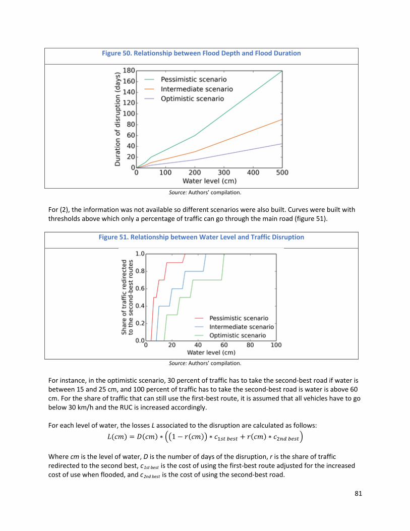
Figure 50. Relationship between Flood Depth and Flood Duration


For (2), the information was not available so different scenarios were also built. Curves were built with thresholds above which only a percentage of traffic can go through the main road (figure 51).

Figure 51. Relationship between Water Level and Traffic Disruption


For instance, in the optimistic scenario, 30 percent of traffic has to take the second-best road if water is between 15 and 25 cm, and 100 percent of traffic has to take the second-best road is water is above 60 cm. For the share of traffic that can still use the first-best route, it is assumed that all vehicles have to go below 30 km/h and the RUC is increased accordingly. For each level of water, the losses L associated to the disruption are calculated as follows:

𝐿𝐿(𝑎𝑎𝑚𝑚) = 𝐷𝐷(𝑎𝑎𝑚𝑚) ∗ ��1 − 𝑚𝑚(𝑎𝑎𝑚𝑚)� ∗ 𝑎𝑎1𝑠𝑠𝑡𝑡 𝑏𝑏𝑏𝑏𝑠𝑠𝑡𝑡 + 𝑚𝑚(𝑎𝑎𝑚𝑚) ∗ 𝑎𝑎2𝑛𝑛𝑑𝑑 𝑏𝑏𝑏𝑏𝑠𝑠𝑡𝑡� Where cm is the level of water, D is the number of days of the disruption, r is the share of traffic redirected to the second best, c1st best is the cost of using the first-best route adjusted for the increased cost of use when flooded, and c2nd best is the cost of using the second-best road.

81

To those losses, the cost of reconstruction is added if D (cm) is higher than 30 days, or the cost of rehabilitation if D(cm) is between 10 and 30 days (table 17). Below 10 days of disruption it is assumed that the road only needs cleaning. These costs of reconstruction, rehabilitation, and cleaning depend on the characteristics of the disrupted link and are multiplied by its number of kilometers. Here it is assumed that reconstruction takes 30 days per km, rehabilitation 10 days per km, and cleaning 2 days per km. During reconstruction or rehabilitation, only a share of traffic can use the road. Since this is uncertain, here again three different scenarios are used (in the optimistic one 90 percent of traffic can use the link during reconstruction; at a slower pace, in the intermediate one 80 percent can use the link; and in the pessimistic one 70 percent of traffic can go through).

Table 17. Assumptions on Construction and Rehabilitation of a Paved Flat Primary Road, after the Flood

Cost per km ($) Time per km (days) Reconstruction 783,225 30 rehabilitation 359,061 10

Source: Authors’ compilation. All those assumptions allow calculating the expected annual losses based on the probability of each event and the costs of disruption associated to each water level. Although probability is incorporated into the calculation, different probability distributions are considered for different potential futures, which maintains the element of decision making under uncertainty. Expected annual losses are calculated for each combination of climate scenario, flood duration scenario, and traffic redirection scenario. Figure 52 shows the expected annual losses for the three clusters of links. For the Pan Americana, the uncertainty on future expected annual losses mainly depends on climate change while for clusters 3 and cluster 5 on the Carretera Central expected annual losses mostly depends on the duration of floods.

82

Figure 52. Expected Annual Losses


For cluster 3 in particular the uncertainty is very high because this section of the road suffers from high flood levels that can lead to full reconstruction of the road if the flood lasts more than 30 days. Given the length of cluster 3 (84 km) the full reconstruction may significantly increase the total cost of disruption. Possible Interventions

Many policy interventions can be implemented to reduce the vulnerability of a link to floods, depending on the severity of the floods the road is exposed to. For relatively low depth floods, the following interventions can significantly reduce costs:

- Upgrading the infrastructure (for instance raising the level of the road or switching from unpaved to paved roads; improve structures and drainage)

- Increasing the frequency of maintenance, frequent controls; clean drainage; reinforce slopes - Implementing traffic rules to make sure the most important vehicles can go through while

others take an alternative route - Adding more capacity (more lanes)

For more severe floods, options include:

- Enlarging the drainage system - Increasing the redundancy of the link by adding alternative routes - Increasing the redundancy of the link by adding multimodality (for example, trains) - Relocating the road

For the Carretera Central’s cluster 5, the costs and benefits of three possible interventions, namely maintenance, improvement of the second-best alternative, and flood-proofing the first-best route are considered (table 18). For the Panamericana’s cluster 1 and the Carretera Central’s cluster 3, because the flood levels are very high, the cost of a flood-proof road is unknown and therefore only maintenance and improvement of the second-best road are considered.

83

Table 18. Cost and Benefits of Different Interventions Costs per km ($) Benefits Cluster 5

(carretera central)

Cluster 3 (carretera

central)

Cluster 1 (panamericana)

Frequent maintenance

95,000 95,000 80,000 Reduction in flood duration by three

Improve second-best road

796,900 796,900 363,300 Second-best road has the same RUC as the first best road—all flood losses disappear

Flood-proof road 2,929,200 ? ? The road never gets flooded—all flood losses disappear

Source: Authors’ compilation. For each intervention, the net present value (NPV) of the investment is calculated as follows:

𝑁𝑁𝑃𝑃𝑁𝑁 = ��−𝑎𝑎𝑡𝑡𝑖𝑖𝑎𝑎𝑖𝑖(𝑎𝑎) + 𝐸𝐸𝐴𝐴𝐿𝐿(𝑚𝑚𝑡𝑡 𝑜𝑜𝑡𝑡𝑎𝑎ℎ𝑖𝑖𝑜𝑜𝑔𝑔)− 𝐸𝐸𝐴𝐴𝐿𝐿(𝑖𝑖𝑜𝑜𝑎𝑎𝑎𝑎𝑚𝑚𝑡𝑡𝑎𝑎𝑜𝑜𝑎𝑎𝑖𝑖𝑡𝑡𝑜𝑜)

(1 + 𝑚𝑚)𝑡𝑡 �30

𝑡𝑡=1

The benefits of the intervention are the difference between expected annual losses when nothing is done (EAL(do nothing)) and expected annual losses with the intervention (EAL(intervention)). Costs include the initial investment cost and yearly maintenance. The discount rate d is 5. Given the uncertainty on the cost of the different interventions, different scenarios are considered, in which costs increase by 50 and in which costs double. Here it is assumed that maintenance can divide flood duration by three. Note that the NPV calculated here does not include all benefits of the investment, and in particular it does not include macroeconomic benefits. However, since the effectiveness of each intervention is different (maintenance only reduces the duration of the flood, it does not prevent all losses), interventions cannot be compared with a cost-effectiveness analysis and the NPV is necessary.

84

Figure 53. NPV of Different Options for Cluster 5 on the Carretera Central


Cluster 5 on the Carretera Central is analyzed first, and three possible options are compared. Figure 53 illustrates the NPV of each options in many different scenarios combining the uncertainty on climate change, flood duration, traffic redirection, and cost of interventions. It shows that in all scenarios, construction of a flood-proof segment is always profitable because the NPV is positive.

Conversely, maintenance and improvement of the second-best road can have a negative NPV in some scenarios. The scenarios which lead to a negative NPV for improvement of the second-best road are characterized by an optimistic or intermediate assumption on flood duration. In other words, in all scenarios that do not follow a pessimistic relationship between flood depth and flood duration, the improvement of the second-best road is too expensive compared to the reduction in flood losses.

For maintenance, the scenarios that lead to a negative NPV are the scenarios with an optimistic assumption on flood duration. Since maintenance reduces the duration of the flood, if the duration is already optimistic maintenance is not useful.

85

Figure 54. NPV of Maintenance and Improved Redundancy for Cluster 3 on the Carretera Central


To choose the best option to be implemented, several criteria can be applied. Here, the chosen criteria is the minimum of the maximum regret across all scenarios. In other words, for each possible future the regret of each option is calculated (as the difference between the NPV of the option and the NPV of the best option for that particular scenario), and then the best option is the one with the lowest possible value for that regret.

For cluster 5, it is very easy because the flood proof road has the highest NPV in all scenarios. Therefore, the flood-proof road is the option with the minimum maximum regret over all scenarios (and the regret is zero). For cluster 3 on the Carretera Central, the two options considered (maintenance and improvement of the second best) have a positive NPV in nearly all scenarios (figure 54). Maintenance has a negative NPV in a few scenarios in which maintenance costs are twice as expensive as in table 18 and in which reducing the duration of the flood has a very small impact because water levels are very high no matter what. Improvement of the second-best road, conversely, has a positive NPV in all scenarios and is the option with the minimum maximum regret (it is the option with the highest NPV in all scenarios).

86

Figure 55. NPV of Maintenance and Improved Redundancy for Cluster 1 on the Pan Americana


Finally, cluster 1 on the Pan Americana (figure 55) is analyzed. Here improvement of the second-best road may have a negative NPV in scenarios in which climate change reduces expected annual losses and in which the duration assumptions is optimistic. Improved maintenance has a positive NPV in all scenarios and could therefore be chosen as the best option in this case. However, its maximum regret is positive and higher than the maximum regret of improving the second-best road, because in scenarios where flood levels remain very high with climate change, improving the second-best road would lead to much higher benefits. The option with the minimum maximum regret therefore remains the improvement of the second-best road, despite a possible negative NPV.33 For cluster 5 in which flood levels are moderate, the best option is to build a flood-proof segment. For clusters 1 and 3, flood levels are so high that the minimum maximum regret option is to improve redundancy. However, the analysis of cluster 1 and cluster 3 would be more complete here if more alternatives were considered. The construction of a flood-proof road may be unrealistic given the very high flood depths. But multimodal alternatives, or the construction of a road elsewhere (in a flood-proof zone) to increase redundancy could be considered. Such analyses will be carried out later with the client when the data is available.

33 The maximum regret of maintenance is $328 million whereas the maximum regret of improving the second-best road is $233 million.

87

V. CONCLUSIONS AND APPLICATIONS

The main contributions of this study are methodological and three fold. First, it proposes, develops, and pilots a practical definition of accessibility that permits the evaluation of both how travel is done and the opportunities which motivate that travel. Second, it uses the developed accessibility framework and the resulting indicators to structure a framework to assess the criticality (or relative importance) of road corridors, segments, or links in a road network. Third, it applies a robust decision-making approach to guide a cost-effectiveness analysis of policy options available when a road network is exposed to unpredictable climate events (decision making model under uncertainty).

--Accessibility -- This study uses infrastructure- and location-based measures to quantify accessibility. Many reasons drive that decision. First is the importance of being able to interpret the results in a manner that allows policy makers to define targets, monitor progress toward their achievement and link the index to concrete policy levers or interventions. Second, data demands—and assumptions made in reaction to data gaps—can be impractical for replicating estimations for many countries at time. For instance, both person- and utility-based measures require either big datasets subject to proprietary (and privacy) restrictions or rely on surveys which are frequently costly and impractical to replicate. In a multicountry evaluation of the accessibility of multicountry or regional corridors, these data restrictions might be insurmountable. Third, it is critical to propose indicators which can be updated regularly and which allow for benchmarking as a mechanism to rank success and infrastructure demands within a country (among provinces for instance) or across countries (in the case of countries belonging to a common economic cluster or treaty). The infrastructure-based measure is easily interpretable and easily replicable. The measure uses cost— one of the most important determinants of whether travel is undertaken—as its primary component. This measure is not rudimentary; however, costs are calculated based on detailed inputs related to road quality, condition, surface type, and other characteristics. Data about these characteristics is normally available for at least the primary network. Determining how costly a trip from an origin to a destination is per kilometer provides an important, albeit rough, indication of how accessible an origin is to a destination. Transport planners traditionally tend to use these measures as they emphasize the stock and quality of infrastructure. The study relies primarily on speed, travel, and the so-called road user costs (as estimated by the Highway Development and Management Model—HMD4) for the infrastructure-based accessibility measure developed.

All accessibility estimates are expressed in ton-km/$, or alternatively vehicle-km/$. This means in practice that accessibility estimates can be broadly interpreted as the potential economic activity (or opportunities for human or economic interaction) unlocked by a unit of transport used over a specific transport network. In other words, the accessibility indicator quantifies the degree of opportunities for interactions between two specific locations given the cost borne by the user to “move” from one location to another. The higher its level the higher the accessibility and with that the better the opportunities for interaction (human or economic exchanges) between two locations, namely cities, ports, airports, or simply areas of interest. The estimated numbers are comparable across countries. Measuring access to and the cost of actual transport services implies that we assess transport infrastructure through a location-specific lens. This involves asking for a specific location in a given

88

country: what is the cost of using the available transport infrastructure? What is the time and distance to the available transport infrastructure? What transport services are available? What is the productive area served by that transport infrastructure? How long and how much would it cost to go from that location to a specific market inside or outside the country?

--Criticality – Given the complexity and size of national road networks, an assessment of each link individually is costly in terms of data needs and computational demands. More importantly, an assessment of the entire network is unnecessary: carefully selected criticality criteria can narrow a road network of hundreds of thousands of links down to several hundred which deserve further analysis. For the identification of critical corridors, the study uses geopolitical, social, and economic criteria. For the assessment of the “level” of criticality, the technique of interdiction is used to estimate the economic, social, and environmental impact of the disruption or degradation of a corridor or link on the overall network; and the proposed accessibilities indicators provide the backbone to connect the network analysis to transport and economic decisions. The proposed method to assess criticality is straightforward and applies the technique of interdiction, a well know approach used in network analysis. In a nutshell, interdiction in this study examines changes in accessibility when individual routes are made unavailable. Therefore, it provides a direct indication of link importance: a large change in accessibility suggests that a route substantially increases the cost of traveling between two places, rendering travel to the same opportunities more expensive. If the loss of a link yields large decreases in accessibility, that link is identified as critical to the functioning of the network.

The difference between the aggregate accessibility indicators of the baseline configuration prior to disruption and the accessibility index for the “modified” configuration for each disrupted link is a key metric of the criticality of that link. A second metric of criticality is the difference between the total number of kilometers of the baseline configuration and the “modified” configuration. The final metric of criticality, also derived from the interdiction technique, is the economic cost of disruption estimated using the change of accessibility multiplied by the traffic.

In sum, criticality is measured as a vector with three values: change in accessibility, change in network length, and change in economic cost.

The proposed methods help in three ways. First, they provide a scientific and objective quantification of the relative importance of corridors, links, and road segments. Second, they offer a framework for prioritization under budgetary and resource constraints. Third, the framework makes the prioritization process transparent and manageable, which is especially important when interests conflict and social or political motivations emerge.

89

--Making Policy Decisions under Climate Uncertainties to Increase Road Network Resilience–

One of the main challenges when preparing this study was to provide a clear set of concepts to frame the analysis. Discerning clear definitions of resilience, vulnerability, and criticality was not an easy task.

In this study criticality is the characterization of the role a specific route in the road network. It captures its relative importance vis-a-vis other routes (or the network as a whole) and can be assessed using geopolitical, social, and/or economic criteria. Reliability refers to the degree of operability of a route under any circumstance. Resilience refers to the capacity of a route (or a system) to recover to status quo after an adverse event.

These three concepts are essential components of the planner’s decision making process when prioritizing interventions and investments, and when designing systems and institutions in support of the existing assets and services. In practice, many of these interventions are assessed in a deterministic environment in which only extreme situations are considered in the design process—or more radically—none are. In reality, however, deep uncertainties and myriad exogenous events can significantly alter the way resources should and will be allocated to avoid—or rather minimize or bound—disastrous losses when the system or the road network, in our case, is exposed to extreme shocks such as a floods, earthquakes, landslides (natural shocks), or other unpredictable shocks to the system, such as political disruptions, transportation-related accidents, and so on.

A fourth key concept, the concept of vulnerability, emerges when the country (or a road network) faces these deep uncertainties. Vulnerability can be defined as the lack of reliability of a route or system when exposed to exogenous hazards, and can be quantified by the level of losses when extreme events occurs. More properly, Taylor and D’Este (2006) draw a distinction between vulnerability and reliability. Whereas reliability depends on infrastructure performance and is measured as the probability that two locations remain connected under any circumstance, “vulnerability is more strongly related to the consequences of link failure, irrespective of the probability of failure” (Taylor and D’Este 2006: 13). Indeed, the large consequences potentially associated with the failure of some network links may make worthwhile those investments that decrease the vulnerability of these links, regardless of the probability of the failure’s occurrence.

Vulnerability can be altered/changed with policy and investment interventions, and responds to the exposure of a network (or part of it) to unpredictable events. That is the starting point the robust decision making analysis. What the study pilots for the case of Peru is a methodology based on Robust Decision Making (RDM) to frame investment decisions in a road network in a world with deep uncertainties. First, like traditional scenario methods, RDM characterizes uncertainty with multiple views of the future. These multiple views are represented analytically by multiple future states of the world. RDM can also incorporate probabilistic information, but rejects the view that a single joint probability distribution represents the best description of a deeply uncertain future. Rather, RDM uses ranges, or more formally sets, of plausible probability distributions to describe deep uncertainty.

Second, RDM uses a robustness rather than an optimality criterion to assess alternative policies. A robustness criterion seeks solutions that are good (though not necessarily optimal) no matter what the future brings. There exist several specific definitions of robustness, but all incorporate some type of satisfying criteria. For instance, a robust strategy can be defined as one that performs reasonably well

90

compared to the alternatives across a wide range of plausible future scenarios. Often there is no single robust strategy but a set of reasonable choices among which decision makers can choose by evaluating the tradeoffs between robustness and other decision criteria, such as costs and feasibility.

This study evaluates the trade-offs—for the critical links among those vulnerable to flood shocks— between (i) the cost of possible transport measures to improve the performance of the link; and (ii) the reliability of the link under different response measures.

--The Way Forward: Implications— The results of this report have important implications for future economic and social analysis, design of operational projects, and policy making.

Future economic and social analysis. Providing a measurement of transport efficiency—or success in expanding coverage—in the form of accessibility would unlock myriad opportunities to evaluate and test the impact that transport interventions, coverage, and quality have on economic growth, productivity, and access to market for the poorest 40 percent of the population, should that be the question of interest. The proposed metric to measure accessibility are concrete, pragmatic, easy to interpret, relatively flexible to adapt to various data availability (provided that the data have a geographic element), and replicable. Various estimation of accessibility can easily be prepared to compare the success of a network in terms of connecting markets, opportunities (jobs), services (heath and educational centers), and broadly mobility of minorities, and integration of geographic areas.

Design of projects. The tools presented are replicable and easy enough in data demands to be used in the design of transport projects. Using the accessibility and criticality approaches in project design would introduce into the decision making the network effect: the impact or relevance of the specific intervention on the network as a whole, in the accessibility of the poor to markets, the accessibility of communities to services, and so on. Moreover, the tools are flexible enough that various spaces can be defined to limit the accessibility analysis to subnational settings.

Policy making. The testing in three countries of straightforward prioritization and cost-effectiveness approaches to decision making, with and without uncertainty has: (i) revealed the value that these tools have for making planning decisions in the transport sector that are climate-change sensitive and informed by concrete elements of past climate events (that while building in the past incidence of uncertain events do not try to predict the future); (ii) unleashed enormous appetite from our counterparts to use the framework in their prioritization processes, including explicit requests for capacity building in tools and knowledge transfer; and (iii) structured the sector-level dialogue among various ministries, sectors, and agencies in the pilot countries.

--Potential Extensions—

The level of accessibility provided by a specific road network is a key component of poverty reduction, economic development, and increased shared prosperity. Accessibility is also a key element to consider in broader discussions of regional integration and bilateral country agreements. In the case of a natural disaster or any unpredictable event which might disrupt the normal functioning of the road network, planning cost-effective/robust road interventions to minimize the economic and social impact of the hazards on intercity and interregional corridors and on critical linkages between remote areas of at-risk

91

populations and centers of social and economic opportunity would ultimately translate into reduced poverty and economic development.

Natural extensions and next steps of this work include, but are not limited to: • Introducing multimodality and other networks (for example, information and communication

technology, ICT) into the analysis. Now, for practical reasons, the analysis is limited to roads. • Using the accessibility measure to structure multicountry dialogue in regional corridors and regional

exchanges. • Estimating accessibility indicators with a more “social” lens to capture the concept of shared

prosperity and spatial disparity among minorities. • Collaborating with labor, health, and education colleagues to estimate accessibility in a way that is

meaningful to their agendas, perhaps learning what is used in their practices to measure efficiency of service provision.

• Scaling up the estimation of the accessibility indicators to other countries, to create a sensible database that allows for cross-country comparison and benchmarking.

92

VI. References

Alonso M.P., M.A. Beamonte, P. Gargallo, and M.J. Salvador. 2014. “Labour and Residential Accessibility: A Bayesian Analysis Based on Poisson Gravity Models with Spatial Effects.” Journal of Geographical Systems 16: 409–39.

Amaral, S., A. M. V. Monteiro, G. Camara, and J. A. Quintanilha. 2006. “DMSP/OLS Night-Time Light

Imagery for Urban Population Estimates in the Brazilian Amazon.” International Journal of Remote Sensing 27 (5): 855–70.

Annema, Jan Anne. 2013. “Transport Resistance Factors: Time, Money, and Effort.” In The Transport

System and Transport Policy, eds. Bert van Wee, Jan Anne Annema, and David Banister, 101–24. Cheltenham: Edward Elgar.

Arvis, J. F., and B. Shepard. 2011. The Air Connectivity Index—Measuring Integration in the Global Air

Transport Network. Washington, DC: World Bank. Baradaran, Siamak, and Farideh Ramjerdi. 2001. “Performance of Accessibility Measures in Europe.”

Journal of Transportation and Statistics 4 (23). Ben-Akiva, M., and S.R. Lerman. 1979. “Disaggregate Travel and Mobility Choice Models and Measures

of Accessibility.” In Behavioural Travel Modelling, eds. D. A. Hensher, and P.R. Sopher, 654–79. London: Croom Helm.

Binswanger-Mkhize, Hans P. and Sara Savastano. “Agricultural intensification : the status in six African

countries,” World Bank Policy Research Working Paper 7116, World Bank, Washington, DC. Bootsma, P.D. 1997. Airline Flight Schedule Development; Analysis and Design Tools for European

Hinterland Hubs. Utrecht: University of Twente. Breheny, Michael J. 1978. “The Measurement of Spatial Opportunity in Strategic Planning.” Regional

Studies 12 (4): 463–79. Briceño-Garmendia, Cecilia, Heinrich C. Bofinger, Diana Cubas, and Maria Florencia Millán-Placci. 2014.

“Connectivity for Caribbean Countries: An Initial Assessment,” World Bank: Washington, D.C. Budde, A., J. de Wit, and G. Burghouwt. 2008. “Borrowing from Behavioral Science: A Novel Method for

the Analysis of Indirect Temporal Connectivity at Airport Hubs.” Air Transport Research Society Conference, June 2008, Athens.

Burger, Martijn, Frank van Oort, and Gert-Jan Linders. 2009. “On the Specification of the Gravity Model

of Trade: Zeros, Excess Zeros, and Zero-inflated Estimation.” Spatial Economic Analysis 4 (2): 1742–72.

Burns, Lawrence D. 1979. Transportation, Temporal, and Spatial Components of Accessibility. Lexington,

Mass.: Lexington Books.

93

Burghouwt, G., and J. de Wit. 2005. “The Temporal Configuration of Airline Networks in Europe.” Journal of Air Transportation Management 11 (3): 185–98.

Burghouwt, G., and R. Redondi. 2009. “Connectivity in Air Transport Networks: Models, Measures, and

Applications.” Quaderni Del Diparimento, Dipartimento di Inggneria Gestionale, Universita’ Egli Studi di Bergamo.

Buys, Piet, Uwe Deichmann, and David Wheeler. “Road Network Upgrading And Overland Trade

Expansion In Sub-Saharan Africa,” World Bank Policy Research Working Paper 4097, World Bank, Washington, DC.

Comisión Ecónomica para América Latina y el Caribe (CEPAL). 1998. Ecuador: Evaluación de los efectos

socioeconómicos del Fenómeno El Niño en 1997–98. México, julio de 1998. Colombia Country Profile. 2008. Economist Intelligence Unit. London, United Kingdom. Cervero, Robert. 2005. “Accessible Cities and Regions: A Framework for Sustainable Transport and

Urbanism in the 21st Century.” Working Paper, UC Berkeley Center for Future Urban Transport. Cervero, R., T. Rood, and B. Appleyard. 1999. “Tracking Accessibility: Employment and Housing

Opportunities in the San Francisco Bay Area.” Environment and Planning A 31 (7): 1259–78. Chen, Yali, Srinath Ravulaparthy, Kathleen Deutsch, Pamela Dalal, Seo Youn Yoon, Ting Lei, Konstadinos

G. Goulias, Ram M. Pendyala, Chandra R. Bhat, and His-Hwa Hu. 2011. “Development of Indicators of Opportunity-Based Accessibility.” Transportation Research Record: Journal of the Transportation Research Board 2255: 58–68.

Clark, D., V. Kozlova, and G. Schaur. 2013. “Supply Chain Uncertainty as a Trade Barrier.” Unpublished

manuscript. Condeco-Melhorado, Ana, Aura Reggiani, and Javier Gut ٕ◌ierez. 2015. “Accessibility and Spatial

Interaction: An Introduction.” In Accessibility and Spatial Interaction, eds. Ana Condeco-Melhorado, Aura Reggiani, and Javier Gut ٕ◌ierez, 1–12. Cheltenham: Edward Elgar Publishing.

Dalvi, M. Q., and K. M. Martin. 1976. “The Measurement of Accessibility: Some Preliminary Results.”

Transportation 5 (1): 17–42. Danesi, A. 2006. Spatial Concentration, Temporal Co-ordination and Profitability of Airline Hub-and-

Spoke Networks. Ingegneria dei Transporti. Bologna, Universita degli Studi di Bologna. de Jong, Gerard, Andrew Daly, Marits Pieters, and Toon van der Hoorn. 2007. “The Logsum as an

Evaluation Measure: Review of the Literature and New Results.” Transportation Research Part A 41: 874–89.

de Jong, Gerard, Marits Pieters, Andrew Daly, Irma Graafland, Eric Kroes, and Carl Koopmans. 2005.

“Using the Logsum as an Evaluation Measure: Literature and Case Study.” Working Paper, Rand Europe, The Netherlands.

94

Dilley, M., Chen, R. S., Deichmann, U., Lerner-Lam, A. L., and Arnold, M. 2005. Natural Disaster Hotspots: A Global Risk Analysis. Disaster Risk Management Series. No. 5. DIPECHO.

Disaster Hotspots: A Global Risk Analysis. Disaster Risk Management Series. No. 5. DIPECHO. Doganis, R., and N. Dennis. 1989. “Lessons in Hubbing.” Airline Business, March 1989, 42–47. Doll , Christopher N.H., Jan-Peter Muller, and Jeremy G. Morley. 2006. “Mapping regional economic

activity from night-time light satellite imagery,” Ecological Economics 57(1):75-92. Dong, Xiaojing, Moshe E. Ben-Akiva, John L. Bowman, and Joan L. Walker. 2006. “Moving from Trip-

based to Activity-based Measures of Accessibility.” Transportation Research Part A 40: 163–80.

Departamento Nacional de Planeación.. 2010. Plan Maestro de Transporte 2010-2032. Bogota,

Colombia. Ebener, Steeve, Christopher Murray, Ajay Tandon, and Christopher C Elvidge. 2005. “From wealth to

health: modelling the distribution of income per capita at the sub-national level using night-time light imagery,” International Journal of Health Geographics 4.

Ecuador Country Profile. 2008. Economist Intelligence Unit. London, United Kingdom. El-Geneidy Ahmed, and David Levinson. 2006. Access to Destinations: Development of Accessibility

Measures. Report #1 in Access to Destinations Study, University of Minnesota, Minneapolis. Elvidge, C.D., E.H. Erwin, K.E. Baugh, D. Ziskin, B.T. Tuttle, T.Ghosh, and P.C. Sutton. 2009. “Overview of

DMSP nightime lights and future possibilities,” Urban Remote Sensing Joint Event. Elvidge, Christopher D., Marc L. Imhoff, Kimberly E.Baugh, Vinita Ruth Hobson, Ingrid Nelson, Jeff Safran,

John B. Dietz, and Benjamin T. Tuttle. 2001. “Night-time lights of the world: 1994-1995,” ISPRS Journal of Photogrammetry and Remote Sensing 56(2):81-99.

Elvidge, C. D., K. E. Baugh, E. A. Kihn, H. W. Kroehl, E. R. Davis & C. W. Davis. 1997. “Relation between

satellite observed visible-near infrared emissions, population, economic activity and electric power consumption,” International Journal of Remote Sensing 18(6):1373-1379.

Feng-Chi, Hsu. 2015. “Global Radiance Calibrated Nighttime Lights Product Readme.” National Oceanic

and Atmospheric Administration. Available at http://ngdc.noaa.gov/eog/dmsp/radcal_readme.txt. Last accessed March 31, 2015.

Fernandez, R., S. Flores Gomez, F. Estrazulas de Sauza, and H. Vega. 2011. “Chapter 6: Supply Chain

Analysis of Exports and Imports of Agricultural Products: Case Studies of Costa Rica, Honduras and Nicaragua.” In Getting the Most out of Free Trade Agreements in Central America, eds. J. H. Lopez, and T. Shankar, 151–81. Washington, DC: World Bank.

Fries, G., and N. L. Duarte. 2012. “Importaciones de Carne de Cerdo a Honduras: Un Analisis de la

Cadena de Suministro.” IFC, December.

95

http://ngdc.noaa.gov/eog/dmsp/radcal_readme.txt

Fries, G. 2012. “Tres Analisis de Cadenas de Suministro: Carne Bovina, Lacteos y Café Organico.” IFC.

March. Furst, Franz, Carsten Schurmann, Klaus Spiekermann, and Michael Wegener. 2000. “Deliverable D15 of

the EU Project Socio-Economic and Spatial Impacts of Transport Infrastructure Investments and Transport System Improvements (SASI).” Dortmund University, Dortmund.

Ghosh, Tilottama, Rebecca L. Powerll, Christopher D. Elvidge, Kimberly E. Baugh, Paul C. Sutton, and

Sharolyn Anderson. 2010. “Shedding Light on the Global Distribution of Economic Activity.” The Open Geography Journal 3: 147–60.

GFDRR. 2010. Disaster Risk Management in Latin America and the Caribbean Region: GFDRR Country

Notes. Washington, DC: World Bank. Grengs, Joe. 2012. “Equity and the Social Distribution of Job Accessibility in Detroit.” Environment and

Planning B: Planning and Design 39:785–800. Guasch, Jose Luis. 2011. “Logistics as a Driver for Competitive in Latin America and the Caribbean.”

Discussion Paper 193, Inter-American Development Bank, Washington, DC. Guerimà, R., S. Mossa, A. Turtschi, and L. A. N. Amaral. 2005. “The Worldwide Air Transport Network:

Anamolous Centrality, Community Structure, and Cities’ Global Roles.” PNAS 102 (22): 7794–99. Guers, Karst, and Bert van Wee. 2013. “Accessibility: Perspectives, Measures, and Applications.” In The

Transport System and Transport Policy, eds. Bert van Wee, Jan Anne Annema, and David Banister, 207–26. Cheltenham: Edward Elgar.

Guers, Karst T., and Bert van Wee. 2004. “Accessibility Evaluation of Land-use and Transport Strategies:

Review and Research Directions.” Journal of Transport Geography 12: 127–40.

Guers, Karst T., and Jan R. Ritsema van Eck. 2003. “Evaluation of Accessibility Impacts of Land-use Scenarios: The Implications of Job Competition, Land-use, and Infrastructure Developments for the Netherlands.” Environment and Planning B: Planning and Design 30: 69–87.

———. 2001. “Accessibility Measures: Review and Applications: Evaluation of Accessibility Impacts of

Land-use Transport Scenarios, and Related Social and Economic Impacts.” National Institute of Public Health and the Environment, The Netherlands.

Gutiérrez, Javier, Ana Condeço-Melhorado, and Juan Carlos Martín. 2010. “Using accessibility indicators

and GIS to assess spatial spillovers of transport infrastructure investment,” Journal of Transport Geography 18(1):141-152.

Hansen, Walter G. 1959. “How Accessibility Shapes Land Use.” Journal of the American Institute of

Planners 25 (2):73–76. Harris, Chauncy D. 1954. “The Market as a Factor in the Localization of Industry in the United States.”

Annals of the Association of American Geographers 44 (4): 315–48.

96

Iacono, Michael, Kevin Krizek, and Ahmed El-Geneidy. 2008. “Access to Destinations: How Close is

Enough? Estimating Accurate Distance Decay Functions for Multiple Modes and Purposes.” Minnesota Department of Transportation, St. Paul, MN.

Iacono, Michael, David Levinson, and Ahmed El-Geneidy. 2008. “Models of Transportation and Land Use

Change: A Guide to the Territory.” Journal of Planning Literature 22 (4): 323–40. IMF (International Monetary Fund). 2013. World Economic Outlook: Transitions and Tensions.

Washington, DC: IMF. Jenelius, Erik. 2010. “User Inequity Implications of Road Network Vulnerability.” Journal of Transport

and Land Use 2 (3/4): 57–73. Jenelius, Erik, Tom Petersen, and Lars-Goran Mattsson. 2006. “Importance and Exposure in Road

Network Vulnerability Analysis.” Transportation Research Part A 40: 537–60. Joseph, Alun E., and Peter R. Bantock. 1982. “Measuring Potential Physical Accessibility to General

Practitioners in Rural Areas: A Method and Case Study.” Social Science & Medicine 16 (1): 85–90. Kincses, Aron, and Geza Toth. 2012. “Geometry of Potential Models.” Regional Statistics 1: 74–89. Koenig, J.G. 1980. “Indicators of Urban Accessibility: Theory and Application.” Transportation 9: 145–72. Kwan, Mei-Po. 2000. “Interactive Geovisualization of Activity-travel Patterns Using Three-dimensional

Geographical Information Systems: A Methodological Exploration with a Large Data Set.” Transportation Research Part C 8: 185–203.

Kwan, Mei-Po. 1998. “Space-Time and Integral Measures of Individual Accessibility: A Comparative

Analysis Using a Point-based Framework.” Geographical Analysis 30 (3): 191–216. Lakshmanan, J.R., and Walter G. Hansen. 1965. “A Retail Market Potential Model.” Journal the American

Institute of Planners 31 (2): 134–43. LaMondia, Jeffrey J., Carey E. Blackmar, and Chandra R. Bhat. 2010. “Comparing Transit Accessibility

Measures: A Case Study of Access to Healthcare Facilities.” Unpublished manuscript. Linneker, B. J., and N. A. Spence. 1992. “Accessibility Measures Compared in an Analysis of the Impact of

the M25 London.” Environment and Planning A 24 (8): 1137–54. Lo, C. P. 2002. “Urban Indicators of China from Radiance-Calibrated Digital DMSP-OLS Nighttime

Images.” Annals of the Association of American Geographers 92: 225–40. Lu, Qing-Chang, Zong-Ren Peng, and Junyi Zhang. 2015. “Identification and Prioritization of Critical

Transportation Infrastructure: Case Study of Coastal Flooding.” Journal of Transportation Engineering. 141(3): 04014082.

97

Luo, Wei, and Fahui Wang. 2003. “Measures of Spatial Accessibility to Health Care in a GIS Environment: Synthesis and a Case Study in the Chicago Region.” Environment and Planning B: Planning and Design 30: 865–84.

Mahadevan, Meera, Nobuo Yoshida, and Larisa Praslova. 2013. “Kyrgyz Republic - Poverty Mapping:

Methodology and Key Findings,” World Bank, Washington, DC. Malighetti P., S. Paleari, and R. Redondi. 2008. “Connectivity of the European Airport Network: ‘Self-help

Hubbing’ and Business Implications.” Journal of Air Transport Management 14: 53–65. Meybeck, M., P. Green, and C. Vörösmarty. 2001. “A New Typology for Mountains and Other Relief Classes: An Application to Global Continental Water Resources and Population Distribution.” Mountain

Research and Development 21 (1): 34–45. MINCETUR. 2015. http://www.peru.travel/about-peru/location-geography-and-climate.aspx. Ministerio de Transporte de la República de Colombia. 2005. “Encuesta Origen-Destino A Vehículos de

Carga Año 2003.” Ministerio de Transportes y Comunicaciones Provias Nacional de la República de Perú. 2011. “Estudio de

Demanda de Carga y Pasajeros 2010.” Morales Sarriera, Javier, Gonzalo Araya, Tomás Serebrisky, Cecilia Briceño-Garmendia, and Jordan

Schwartz. 2013. “Benchmarking Container Port Technical Efficiency in Latin America and the Caribbean: A Stochastic Frontier Analysis.” Policy Research Working Paper 6680, World Bank, Washington, DC.

Moreira, Mauricio Mesquita, Juan Blyde, Christian Volpe, and Danielken Molina, eds. 2013. Too Far To

Export: Domestic Transport Costs and Regional Export Disparities in Latin America and the Caribbean. Washington, DC: Inter-American Development Bank.

Murray, Alan T., and Tony H. Grubesic. “Overview of Reliability and Vulnerability in Critical

Infrastructure.” In Critical Infrastructure: Reliability and Vulnerability, eds. Alan T. Murray, and Tony Grubesic, 1–8. New York: Springer.

Niemeier, Debbie. 1997. “Accessibility: An Evaluation Using Consumer Welfare.” Transportation 24:

377–96. OECD (Organisation for Economic Co-operation and Development). 2013. Latin American Economic

Outlook 2014: Logistics and Competitiveness for Development. Paris: OECD jointly with the Development Bank of Latin America (CAF) and United Nations Economic Commission for Latin America and The Caribbean (UN-ECLAC).

Osborne, T., M. C. Pachon, and G. E. Araya. 2013. “What Drives the High Price of Road Freight Transport

in Central America?” Unpublished working paper. Papa, Enrica, and Pierluigi Coppola. 2012. “Gravity-Based Accessibility Measures for Integrated

Transport-Land Use Planning (GraBAM).” University of Naples Federico II, Naples.

98

Pokharel, Ramesh, and Hitoshi Ieda. 2013. “Prioritization of Road Network Sections to Upgrade Dry

Weathered Condition: An Accessiblity Approach in Rural Areas of Nepal.” Proceedings of the Eastern Asia Society for Transportation Studies 9: 1–11.

Rautela. P., and S. Pant. 2007. “Research Communications.” Current Science 92 (8), April 25, 2007. Rodriguez, Jean-Paul. 2013. “Spatial Interactions and the Gravity Model.” In The Geography of Transport

Systems, Hofstra University, Department of Global Studies & Geography. http://people.hofstra.edu/geotrans/eng/methods/ch5m1en.html. Last accessed February 27, 2015.

Rosca, Eugen, Mihaela Popa, and Florin Rusca. 2008. “Transport Networks Reliability and Vulnerability in

Large Urban Areas.” Mechanics Transport Communications 3(0235):I26-I31. Santos Silva, J. M. C., and Silvana Tenreyo. 2006. “The Log of Gravity.” The Review of Economics and

Statistics 88 (4): 641–58. Samad, T., N. Lozano-Gracia, and A. Panman, eds. 2012. Colombia Urbanization Review: Amplifying the

Gains from the Urban Transition. Washington, DC: World Bank. Scott, Darren M., David C. Novak, Lisa Aultman-Hall, and Feng Guo. 2006. “Network Robustness Index: A

New Method for Identifying Critical Links and Evaluating the Performance of Transportation Networks.” Journal of Transport Geography 14: 215–27.

Serebrisky, Tomás. 2012. Airport Economics in Latin America and the Caribbean: Benchmarking,

Regulation, and Pricing. Washington, DC: World Bank. Shepherd, Ben. 2012. “The Gravity Model of International Trade: A User Guide.” United Nations ESCAP,

United Nations, New York. Simmonds, D., and N. Jenkinson. 1993. “Regional Economic Impacts of the Channel Tunnel.” PTRC

Summer Annual Meeting. Proceedings of Seminar A, Manchester, PTRC, London, 191–204. ———. 1995. “The Impact of Changing Transport Services in Europe,” PTRC Summer Annual Meeting.

Proceedings of Seminar A, Manchester, PTRC, London, 191–204. Sohn, Jungyul. 2006. “Evaluating the Significance of Highway Network Links under the Flood Damage: An

Accessibility Approach.” Transportation Research Part A 40: 491–506. Song, Shunfeng. 1996. “Some Tests of Alternative Accessibility Measures: A Population Density

Approach.” Land Economics 72 (4): 474–82. Taylor, Michael A. P., and Glen M. D’Este. 2007. “Transport Network Vulnerability: a Method for

Diagnosis of Critical Locations in Transport Infrastructure Systems.” In Critical Infrastructure: Reliability and Vulnerability, eds. Alan T. Murray, and Tony Grubesic, 9–30. New York: Springer.

99

http://people.hofstra.edu/geotrans/eng/methods/ch5m1en.html

Taylor, Michael A.P., Somenahalli V.C. Sekhar, and Glen M. D’Este. 2006. “Application of Accessibility Based Methods for Vulnerability Analysis of Strategic Road Networks.” Network and Spatial Economics 6: 267–91.

Taylor, Michael A. P., and Susilawati. 2012. “Remoteness and Accessibility in the Vulnerability Analysis of

Regional Road Networks.” Transportation Research Part A 46 (5): 761–71. Ukkusuri, Satish V., and Wilfredo F. Yushimito. 2009. “A Methodology to Assess the Criticality of

Highway Transportation Networks.” Journal of Transportation Security 2: 29–46. van Wee, Bert, Michel Hagoort, and Jan Anne Annema. 2001. “Accessibility Measures with

Competition.” Journal of Transport Geography 9: 199–208. Veldhuis, J. 1997. “The Competitive Position of Airline Networks.” Journal of Air Transport Management

3 (4): 181–8. Vickerman, R.W. 1974. “Accessibility, Attraction, and Potential: A Review of Some Concepts and Their

Use in Determining Mobility.” Environment and Planning A 6 (6): 675–91. Winsemius, H.C., L.P.H Van Beek, B. Jongman, P.J. Ward, and A. Bouwman. 2013. A Framework for

Global River Flood Risk Assessments. Hydrology and Earth System Sciences 17: 1871–92. Weibull, Jorgen. 1976. “An Axiomatic Approach to the Measurement of Accessibility.” Regional Science

and Urban Economics 6: 357–79. Wilson, A.G. 1970. Entropy in Urban and Regional Modelling. London: PION. Wilson, A.G. 1967. “A Statistical Theory of Spatial Distribution Models.” Transportation Research 1 (3):

253–69. World Bank. 2011. Analysis of Disaster Risk Management in Colombia: A Contribution to the Creation of

Public Policies. Washington, DC: World Bank. ———. 2009. Reshaping Economic Geography. Washington, DC: World Bank. ———. 2007. “HDM-4 Road Use Costs Model Documentation Version 1.10.” World Bank Technical

Documentation, World Bank, Washington, DC. ———. 2012. Central America Logistics Platform. LCSSD Economics Team, Sustainable Development

Department of the Latin American Region. ———. 2013a. Latin American and the Caribbean as Tailwinds Recede. Semiannual Report, Office of the

Regional Chief Economist, April 2013. ———. 2013b. LAC Equity LAB. Latin American Vice-presidency, Poverty Department available

at http://go.worldbank.org/7N73WK4HI0. ———. 2013c. Enterprise Surveys. Available at http://www.enterprisesurveys.org/.

100

http://go.worldbank.org/7N73WK4HI0

http://www.enterprisesurveys.org/

———. 2012. “Agro-Logistics in Central America: A Supply Chain Approach.” Background Paper. ———. 2013. Planning, Connecting, and Financing Cities Now: Priorities for City Leaders. Washington,

DC: World Bank. ———. 2011. Analysis of Disaster Risk Management in Colombia: A Contribution to the Creation of

Public Policies. Washington, DC: World Bank. WEF (World Economic Forum). 2014. The Global Competitiveness Report 2014—2015: Full Data Edition.

Geneva: WEF. Zhao, Yun. “Assessing the Impact of Potential Bridge Collapse on Road Network Vulnerability: A Case

Study in Oklahoma.” Unpublished manuscript (thesis).

101

VII. ANNEXES: Spatial Disparities through the Accessibility Lens

A) Annex 1. Inventory of GIS Datasets

The study comes with a strong public good component. In order to carry out the analysis, a Geographic Information System (GIS) platform has been created by compiling and curating existing spatial datasets, primarily from public sources. Some limited distribution datasets may also be included. A focus will be on standardization across countries, although country or region-specific datasets will also be incorporated where possible.

In the GIS platform, all key production activities, physical infrastructure stocks, natural resource endowments, and socioeconomic and demographic indicators are mapped at the smallest relevant geography. In the resulting database, information may be represented by points, areas or extents, lines, or gridded surfaces, at a mix of spatial resolutions or scales. A network-node structure is employed in order to bring the different feature types into a common analytical framework. For example, the potential productivity of a particular crop is a gridded surface that can be aggregated to a network node using a minimum-travel-cost allocation grid.

A core component of the GIS database is the construction and validation of a functional road transport network, with clean topological relationships. This is a frequently overlooked but significant task, critical for any analysis with the objective of modeling flows. It will enable researchers to evaluate current infrastructure constraints, model alternative scenarios, and potentially look at redundancy in the system.

The primary goal of this effort is to provide easier access to data and documentation for researchers involved in this study, the GIS database can hopefully be useful for futures research activities as well as Bank operations and planning activities.

The data can be roughly groups in 4 areas:

1. Economic and demographic data. Agricultural surveys, household surveys, business surveys, and internationally available geo-reference databases such as International Food Policy Research Institute’s (IFPRI’s) Agriculture Spatial Production Allocation Model (SPAM).

2. Environmental and natural resource. Country-specific literature and data used for poverty maps. It selectively includes available census data and draw from internationally available GIS-population databases.

3. Transport and infrastructure data. Road surveys are an essential input and come from client countries via our on-going operational engagement. For railways, ports, and airports data has been made available by operational teams. Google Earth, country-specific satellite imagery, and digitized maps are also good sources of data. Additional sources include the Latin America and the Caribbean Sustainable Development Department’s Port Database and Containerization International Yearbooks for port location and capacity.

4. Other/comprehensive geographic data. Administrative boundaries, standard names, and point of interests

i. Economic and Demographic Data

Global Databases

i. IFPRI SPAM

IFPRI’s SPAM is a methodology that transforms crop production statistics available at the administrative level to much finer spatial disaggregation (5 arc-minute gridded cell < 10 kilometers [km]). To allow for the cross entropy estimation, other input data include land cover, land use, crop suitability assessment, population density, distance to market centers, as well as existing knowledge of crops’ geographic distribution.

The significance of SPAM is that it allows for visualizing and analyzing crops’ spatial heterogeneity within the administrative units. In the current version of the dataset (2000), 20 crops are included for 422 admin level 1 units and 8,517 admin level 2 units in the Latin American region.

ii. Global Agro-ecological Zone (GAEZ)

GAEZ is a long-term project and continuously evolving product of Food and Agriculture Organization of the United Nations (FAO) and the International Institute for Applied Systems Analysis that started in 2000. It is the first database built to assess agricultural resources and potential for the entire globe, covering five thematic areas:

• Land resources, terrain resources, water resources, land cover, protected areas, and a few demographics data

• Climatic indicators including thermal regimes and moisture regimes • Suitability and potential yields for 49 crops under different scenarios of input levels and

historical, current, and future climate conditions • Actual crop yields, harvested area, and production for 23 commodities in 2000 and 2005 • Yield and production gaps

The GAEZ assessment is widely used by the academia and international organizations as it provides maximum potential and biophysically attainable yields and suitable crop areas. The dataset is composed of 5 arc-minute resolution map and tables aggregated from various geographic levels (from global to subnational administrative levels).

iii. Defense Meteorological Satellite Program–Operational Linescan System (DMSP-OLS) Nightlights

DMSP satellite flies in a sun-synchronous orbit and orbits the earth 14 times a day. The OLS is the main sensor equipped on the platform. Since OLS can capture the lowest levels of radiation thanks to its photoelectric zooming capacity, the nighttime lights data from the sensor can be used to measure changes in human activities over time. Datasets currently exist for years from 1992 to 2012 and come in the form of average Digital Number (DN) values per year. The digital number is an integer between 0 and 63; 0 represents completely dark areas while dense areas with more lighting at night are closer to 63. The spatial resolution of the pixel is 30 arc-seconds (1 km).

iv. Global Subnational Prevalence of Child Malnutrition

The Global Subnational Prevalence of Child Malnutrition dataset, produced by the Columbia University Center for International Earth Science Information Network (CIESIN), consists of estimates of the percentage of children underweight who are below age 5. Data are reported for the most recent year with subnational information available at the time of development (between 1990 and 2002). The dataset includes a shapefile of percentage rates and grids of rates (per thousand).

v. Global Subnational Infant Mortality Rates

Global Subnational Infant Mortality Rates provides estimates of infant mortality rates for the year of 2000. Infant mortality rate is defined as the number of children who die before their first birthday for every 1,000 live births. The dataset is prepared by the CIESIN and includes a shapefile of rates, births, and deaths, as well as a raster file of rates (per 10,000).

vi. Environmental Systems Research Institute (Esri) World Cities

World Cities, depicted as points in the shapefile, is a layer prepared by ESRI. Additional attributes available are “Admin Name,” Country Name,” “Country Code,” “Population Rank,” “Population Class,” and “Port Identification Number.” Information used in constructing the dataset was collected in 1993, 1994, 1996, 1999, 2000, 2001, and 2003.

vii. Henderson World Cities Database

Henderson World Cities Database is a vector shapefile pinpointing the location of the majority of world cities with additional information about the cities’ population in 1960, 1970, 1980, 1990, and 2000.

Country Specific Data Sets

i. Enterprise Surveys

The Enterprise Surveys are global surveys conducted by the World Bank covering small, medium, and large companies established mostly in the urban areas. The firms sampled are in the nonagricultural private sector, which includes the manufacturing sector, service sector, transportation, and construction sector. There are two rounds of surveys published so far—in 2006 and 2010. The survey design and implementation follow a uniformed methodology, thus allowing indicators generated from the surveys comparable across countries and years.

In Latin America and the Caribbean (LAC), 15 and 31 countries are included in the Enterprise Survey in 2006 and 2010 respectively. Through in-person interviews, Enterprise Surveys ask firm managers and owners qualitative and quantitative questions on topics such as infrastructure, trade, finance, regulations, taxes, business licensing, corruption, crime, and perceptions about obstacles to doing business. Therefore, the indicators provide a comprehensive overview of the firms’ business environment and productivity in each surveyed county. More importantly, the indicators are geo-referenceable as the values aggregated by location (that is, urban municipalities) are available.

ii. Socio-Economic Database for Latin America (SEDLAC) Household Surveys

SEDLAC database holds statistics on poverty, inequality, welfare, income, and infrastructure variables from 24 LAC countries computed from the main household surveys. All variables are harmonized using a homogeneous methodology and, thus, allow for cross-country comparison. In addition to the summary statistics, we have access to the harmonized raw surveys (microdata) for each country. Geographic information (that is, subnational region) for all the households surveyed is also provided in the survey.

iii. Demographics and Health Surveys (DHS)

The DHS is a project funded by the U.S. Agency for International Development (USAID) that collects data on and studies population, health, human immunodeficiency virus (HIV), and malnutrition. In the LAC region, surveys have been conducted for 12 countries including Bolivia, Brazil, Colombia, Dominican Republic, Guatemala, Guyana, Haiti, Honduras, Mexico, Nicaragua, Paraguay, and Peru in various years. A total of 24 indicators are available at the subnational level in the GIS data format.

iv. Small Area Estimates of Poverty and Inequality (CIESIN)

The Small Area Estimates of Poverty and Inequality dataset consists of poverty, inequality, and related measures for subnational administrative units, available in both spatial and tabular formats. The variables are extrapolated from national census and survey data using small area estimates techniques. Available maps include countries like Bolivia, Dominican Republic, Ecuador, Guatemala, Honduras, Nicaragua, and Paraguay in the LAC region.

v. Poverty and Food Security Case Studies (CIESIN)

The Poverty and Food Security Case Studies dataset comprises small area estimates of poverty, inequality, and food security measures for subnational administrative units in Mexico and Ecuador. The measures are presented in both spatial and tabular forms.

ii. Environmental and Natural Resource Data

Global Databases

i. Global Risk Data Platform (GDRP) Multiple Hazard Index

This global dataset, available both in vector and raster formats, provides an estimate of potential risks posed by multiple natural hazards (that is, tropical cyclone, flood, and land slide). The unit of the index is from 1 (low) to 5 (extreme). It is product of UN Environment Program (UNEP)/Global Resource Information Database (GRID)-Europe for the Global Assessment Report on Risk Reduction.

ii. World Database on Protected Areas (WDPA) Protected Area

The WDPA, a joint effort between the UNEP and the International Union for Conservation of Nature, is the only global database of marine and terrestrial protected areas. Each protected area must have at a minimum 14 attributes, including “Name,” “Country,” “Designation,” “Type,” “Status,” and so on. Additional attributes available are “Original Name,” “Subnational Location,” “Governance Type,” “Management Authority,” “International Standard Category,” and so on.

iii. Mineral Resource Data System (MRDS)

MRDS is a shapefile of metallic and nonmetallic mineral resources throughout the world, made available by the U.S. Geological Survey. It has a global coverage and contains 18,000 mineral sites for the LAC region. Other than geographic characteristics of the sites, MRDS dataset contains valuable information such as: general type of deposits at the site (for example, vein, hot spring, placer, stratabound, sedimentary, and so on), type of operation at the site (that is, surface, processing plant, placer, and underground), magnitude of production (that is, small, medium, large, and undetermined), status of development of the resource/site (that is, producer, occurrence, past producer, plant, and prospect), type of commodities present, work type (that is, surface or underground), name of ore mineral found in this deposit, name of gangue mineral found in the deposit, geochemical alteration done to the site, name of the person who entered information about the site, lithologic and stratigraphic information regarding the host rocks for the ore, geological description at or near the deposit, description of the tectonic setting within which the deposit is found, year of site discovery, first production and last production, and entities associated with the discovery of the resource. However, it is worth noting that for the deposits in the LAC region, the majority of the sites’ operation types are unknown.

iv. Digital Elevation Model (SRTM 30 m)

SRTM30 is a near-global (80 percent of the total landmass) digital elevation model (DEM) using data from the Shuttle Radar Topography Mission (SRTM) and the U.S. Geological Survey’s GTOPO 30 dataset. SRTM30 has high spatial resolution at 30 meter and each cell indicates the elevation of the area represented.

iii. Transport and Infrastructure Data

This might have different sources. Road surveys are an essential input and would come from client countries via our on-going operational engagement. For railways, ports, and airports data can be made available by operational teams. Google Earth, country-specific satellite imagery, and digitized maps are also good sources of data. Additional sources include the LCSSD Port Database and Containerization International Yearbooks for port location and capacity.

Global Databases

i. Global Roads Open Access Dataset

The Global Roads Open Access Dataset Version 1 (gRoadsv1) combines the best available roads data by country into a global road coverage (also to some extent topologically integrated). The database was compiled by the CIESIN from multiple sources; consequently, the dates representing the road networks range from 1980 to 2010 depending on the country (although most countries did not provide this information). There are numerous useful fields (for example, “Number of Lanes,” “Surface Type,” “Speed Limit,” “Class,” and so on.) listed as attributes, however, at this point, all records appear as empty.

ii. World Port Index

The World Port Index, available in a vector file format, displays the location and characteristics of major ports and terminals around the globe. The dataset not only has roughly 3,700 ports documented but is also rich in content; 31 attribute types include, for example, “Sailing Direction,” “Harbor Size,” “Harbor Type,” “Maximum Size Vessel,” and “Crane/Lifts.”

iii. OpenFlights Airports

The OpenFlights Airports Database is available in a tabular format with information regarding airports locations (Latitude and Longitude), city and country of the airport, airport’s International Air Transport Association (IATA)/Federal Aviation Administration (FAA) codes, altitude, time zone, and daylight savings time of the airport location. In the latest version as of January 2012, 6,977 airports in total are registered in this dataset.

iv. ESRI Rail Network for the LAC Region

This is a subset of World Railroads dataset (shapefile) published by ESRI in 2010. The polyline features delineate the railway network in the LAC region. Attribute information such as name of the rail, country, and administrative units (level 1 and level 2) intersected by the rails is also available.

v. Open Street Map (OSM)

OSM is a collective project that utilizes Global Positioning System (GPS) and aerial photography to create an editable map of the World. OSM data is available for 31 countries in the LAC region. For the road networks, features are classified into different types—mostly “primary,” “secondary,” “tertiary,” “track,” and “residential.” Other important information for roads is not available. Additionally, the OSM dataset depicts the geographic location and shape of each country’s water body, forests, point of interests, and coastline.

Country Specific Data Sets

i. Peru Transport Network

The Peru road data, obtained directly from Peru’s Ministry of Transport and Communication, has condition and surface type for the entire road network (that is, national, departmental, and vecinal). The reference year of the dataset is December 2013. Peru’s road network is very complete and contains the complete set of attribute information (that is, class, condition, and surface type).

An additional spatial dataset consists of Peru’s airports, ports, and road network (tolls, national, departmental, and local roads). The data is provided by Peru’s Ministry of Transport and Communications. Attributes information for the ports data include name of the port, port’s management company, public-owned or private-owned, type of the terminal, operation status, maritime, fluvial or lacustrine, and so on. Information related to airports includes the name of the airport, operational status, residing departments, and administrations that manage the airports. Regarding the road networks, pavement condition is available for all three types of roads; there are three categories for the local roads (that is, rural) and five for the national (that is, interstate highway) and departmental roads (that is, secondary). Additionally, road condition (that is, bad, regular, and good) is specified for the national road.

ii. Colombia Road Network

A full network of Colombia came from Instituto Nacional de Vias (2010). That network, however, did not have attributes such as condition and surface types. These attributes were transferred to the primary road class of Colombia’s full network a separate shapefile was obtained from the Instituto Geográfico Agustin Codazzi.

iii. Ecuador Road Network

For Ecuador, the national road data was shared by the Inter-American Development Bank (IDB) and has surface condition and pavement type. Another shapefile, representing the remainder of Ecuador’s road network, was downloaded from the website of Ecuador’s Instituto Geográfico Militar with a reference year of 2005. The road network is classified into three classes: primary, secondary, and local. Surface type information is available for all three classes, but road condition is missing.

iv. Other/Comprehensive Geographic Data

i. Global Administrative Boundaries (GADM)

GADM version 2.0 (2012) is a shapefile delineating the administrative boundaries for the world. Administrative areas classified in this dataset are countries and lower level subdivisions such as provinces, departments, counties, and so on. Municipality boundaries (admin level 2) for several large counties in the LAC region are also available.

ii. Global Map V.2

Global map is a raster dataset with 1 km resolution covering the earth’s surface. There are eight thematic layers: “Boundaries,” “Drainage,” “Transportation,” Population Centers,” Elevation,” Land Cover,” “Land Cover,” “Land Use,” and “Vegetation.” All eight layers of the Global map version 2 is released in 2013.

iii. ESRI World Gazetteer

World Gazetteer represents the locations and proper names for point of interest around the World. General features included are airports, coastal features, drainage features, islands, land features, ocean features, political features, populated places, location, oceans, and transportation. Information used in constructing the dataset was collected in 1992, 1993, 1994, 2000, and 2002.

B) Annex 2: Consolidation of Road Network Datasets

GIS road datasets for Peru, Ecuador, and Colombia were compiled from the respective country road agencies or institutes of geography but the level of granularity, geometry, and road attributes vary significantly. Table 1 summarizes the availability of major attributes (for example, road class, condition, and surface type) and the source and year of the road vector data for Peru, Ecuador, and Colombia, respectively.

Table 1. Major Attribute Availability and Source of GIS Road Data for Peru

Country Class Condition Surface Type GIS Source Other Source

Peru • National • Departmental • Vecinal

• National • Departmenta

l • Vecinal

• National • Departmenta

l • Vecinal

Ministry of Transport and

Communication 2013

Ecuador • Primary • Secondary* • Local*

• Primary • Primary • Secondary* • Local*

IDB 2012 Instituto

Geografico Militar 2005*

Colombia

• Primary • Secondary • Carreteable • Camino

• Primary* • Primary* National Roads

Institute 2010

Instituto Geografico

Agustin Codazzi 2006*

Source: Authors’ compilation. Note: *indicates the data is collected and compiled from the secondary source.

In order to produce an integrated, multicountry road network suitable for modeling regional logistics and trade routes, the values in each field (for example, condition, surface type) were standardized across the three countries using a correspondence table or “field mapping” (table 2).

Table 2. Standardization of Major Attributes Network Classification Condition Surface Class Primary Secondary Tertiary Good Regular Bad Paved Unpaved

PER

Nacional Department Vecinal

Buena

Muy Buena

Regular Sin Data

Proyectado

Malo Muy Malo

Asfaltado Afirmado

Sin Afirmar Trocha

Sin Data

COL Primary Secondary Camino Carreteable Bueno Regular

Sin Data Malo Pavimentado Afirmada

Sin Afirmar Sin Data

ECU

Primary Secondary Local Bueno Regular Sin Data Malo Pavimento

No Pavimento

Otro No Aplica No Tiene Temporal


There are evident data gaps. For Ecuador’s secondary and tertiary networks condition information is missing. For Colombia no data on condition was available. To maximize the use of data some

assumptions were made. The actual values of these attributes can be corrected if and when the information becomes available (table 3).

Table 3. Some Assumptions Were Made to Fill Data Gap (coverage of GIS road data by attribute)

Network Type Country

GIS Coverage

of Reported Network

kms %

Surface Type (Paved/Unpaved)

Condition (Good/Fair/Poor)

# of Lanes

Primary Colombia 100 √ √ 4 Ecuador 100 √ √ √

Peru 100 √ √ 4

Secondary Colombia 11 unpaved fair 2 Ecuador 100 √ fair 2

Peru 100 √ √ 2

Tertiary Colombia 40 unpaved fair 2 Ecuador 100 √ fair 2

Peru 100 √ √ 2

Source: Instituto Nacional de Carreteras (2012) and Instituto Geográfico Agustín Codazzi (2006) for Colombia; Inter-American Development Bank (2012) and Instituto Geográfico Militar (2005) for Ecuador; and Ministerio de Transportes y

Comunicaciones (2013) for Peru. Note: √ = data available; italics = characteristic assumed.

Once the country datasets were assembled, road features extending into neighboring countries were clipped based on the border lines delineated by the World Bank Country Boundary Polygon shapefile. For network modelling purposes, the integrated network was planarized to ensure that the “nodes” are specified at the crossing between arcs. This allows vehicles to switch from one arc to another when modelling the routing. Then the network was dissolved to reduce the number of features that are contiguous and have identical attributes. A number of limitations associated with the input datasets and the methods used in this analysis should be taken into account in the interpretation of results.

• Scale of roads. The scale of the source data (that is, the level of detail) for roads is unknown, but there are obvious differences between the countries and in comparison with large-scale datasets such as OSM. The smaller the scale, the less likely the features in the GIS data will accurately represent the geometry of the roads on the ground. As a result, the total kilometers calculated based on the GIS data will deviate, to some degree, from the officially reported statistics. In figure 1, scale makes a big difference in the calculated sinuosity index value.

• Spatial resolution of elevation model. The spatial resolution of the elevation model also presents a challenge, particularly with respect to the average width of roads. Figure 1 shows a road drawn with a width of 7 meters (m), approximately one third of the size of an elevation cell. In this case, extracted z-values will be affected by roadside features, particularly in areas of high relief.

• Segmentation. In the [terrain] analysis, road characteristics are calculated by segment, which is defined somewhat arbitrarily according to the network geometry. While the start and end of a

segment may not necessarily define a homogenous feature, errors in network geometry only exacerbate the problem

Figure 1. Examples of Challenges with Input Datasets

a. Scale Difference between gROADS and Open Street Map

b. Spatial Resolution of Digital Elevation

Model

c. Segmentation Example


GIS versus National Roads Data To validate the GIS road networks in use, descriptive statistics emerging from those datasets were compared to statistics published by the road agencies of Colombia, Ecuador, and Peru. The road length in kilometers presented for the GIS detests is generated based on the geometry of the vector files using

Universal Transverse Mercator (UTM) 18S projection coordinate system and Geographic Coordinate System World Geodetic System 1984. Total road length and road length by class (primary, secondary, and tertiary) for each country is presented in table 4. In each road class, Peru has the most kilometers. Ecuador is last in terms of road length with a total of 44,792 km. When comparing the total kilometers to official statistics for the respective counties (table 4 and figure 2), the deviation is small for Ecuador and Peru. But in the case of Colombia, there is a significant gap. The size of Colombia’s road network is the largest among the three countries with a total of 202,695 km. However, the GIS road data only captures 1/3 of the total with 79,698 km. Further examination by road class reveals that the missing lengths solely fall under the secondary and tertiary roads.

Table 4. Road Length (km) by Class, GIS

Primary Secondary Tertiary Total Colombia 17,965 4,864 56,869 79,698 Ecuador 9,555 17,093 18,145 44,792

Peru 26,870 29,123 108,049 164,044 Source: Authors’ compilation.

Figure 2. GIS Road Network Versus Reported Road Networks a. Colombia

b. Ecuador

c. Peru

Source: Authors’ compilation. Note: (a) Road length by class (km), GIS vs. official statistics for Colombia; (b) total road length (km) vs. International Road Federation statistics for Ecuador; and (c) road length by class (km), GIS vs. official statistics for Peru.

0

50,000

100,000

150,000

200,000

GIS INVIAS, 2012

0

10,000

20,000

30,000

40,000

GIS IRF, 2010

GIS IRF, 2010

0

50,000

100,000

150,000

GIS MTOC, 2012

C) Annex 3: Using HDM-4 to Calculate Road User Costs and Average Road Speeds

The Highway Development and Management Model (HDM-4) uses road characteristics and vehicle fleet data to compute unit road user costs. HDM-4 uses two categories of inputs: data related to road characteristics and data related to vehicle fleets. Road characteristics are defined at the link level. For the purposes of our analysis, vehicle fleet data is compiled at the national level. Road Characteristics While the model permits inclusion of many different road variables, six road characteristics which were either available or able to be calculated from geospatially referenced road network data are used as inputs and the basis for assumptions about other inputs. These six characteristics are: network type, terrain class, surface type, pavement condition, traffic class, and number of lanes. Network Type Network type refers to primary, secondary, and tertiary networks and is provided in the geospatial road network data obtained from the governments of Colombia, Ecuador, and Peru. Network type, in conjunction with surface type and pavement condition (see below), was used to make assumptions of road roughness (on the International Roughness Index), an important contributor to road user costs. Network type was also used to make assumptions about carriageway width.

Table 5. Road Roughness (IRI, m/km) Paved Unpaved

Good Fair Poor Good Fair Poor Primary 2 5 10 Primary 10 14 18

Secondary 3 6 11 Secondary 12 16 20 Tertiary 4 7 12 Tertiary 14 18 22

Carriageway Width (m)

Primary 7.0 Secondary 6.0

Tertiary 5.0 Source: Authors’ compilation.

Terrain Class Terrain class refers to seven different topological categories: straight and level; mostly straight and gently undulating; bendy and generally level; bendy and gently undulating; bendy and severely undulating; winding and gently undulating; and winding and severely undulating. Terrain class was calculated from geospatial network data and used to make assumptions about four road characteristics:

• Rise and fall (m/km). Sum of the absolute values of total vertical rise and total vertical fall of the original ground, in meters, along the road alignments over the road section in either direction divided by the total section length, in kilometers.

• Number of rise and fall per km (#). Number of rises plus the number of falls, as defined on the computation of the rise and fall of a road section, per kilometer of a road section.

• Horizontal curvature (deg/km). Weighted average of the curvatures of the curvy sections of the road, the weights being the proportion of the lengths of curvy sections. It units are degrees/km.

• Altitude (m). Altitude of the terrain (the average elevation of the road above the mean sea level, in meters).

Table 6. Road Geometry

Rise and Fall

(m/km)

# of Rise/Fall per km

Horizontal Curvature (deg/km)

Super_ Elevation

(%)

Altitude (m)

Speed Limit

(km/hr)

Speed Limit Enforcement

(#)

Roadside Friction

(#)

NMT Friction

(#)

Straight and level 1 1 3 2.0 0 110 1.10 1.00 1.00 Mostly straight and gently

undulating 10 2 15 2.5 0 100 1.10 1.00 1.00

Bendy and generally level 3 2 50 2.5 0 100 1.10 1.00 1.00 Bendy and gently undulating 15 2 75 3.0 0 80 1.10 1.00 1.00

Bendy and severely undulating 25 3 150 5.0 0 70 1.10 1.00 1.00

Winding and gently undulating 20 3 300 5.0 0 60 1.10 1.00 1.00

Winding and severely undulating 40 4 500 7.0 0 50 1.10 1.00 1.00


Estimates are derived for each of these characteristics, with the exception of horizontal curvature, using GIS for every road in the digital road datasets. To capture essential characteristics in the horizontal dimension, we use a sinuosity index (SI), defined as the ratio of the actual length of a road segment to the distance between the endpoints. The SI for a perfectly straight segment would be 1, increasing with the number and severity of curves. There are two distinct approaches to deriving road characteristics using GIS: landscape classification and linear feature extraction. In the landscape approach, gridded elevation data is used to classify the average roughness or change in elevation within a fixed or moving window. Roads are then assigned the terrain type that is crossed by the majority of the road length, or further segmented according to the grid structure of the terrain data. The final step is to relate terrain type to the input classes required by HDM-4. Figure 3a illustrates the landscape, or neighborhood approach. The second approach, linear feature extraction, involves extracting elevation data at fixed intervals along the line and directly computing the road characteristics required for HDM-4. Basic steps required for this approach are presented in figure 3b.

Figure 3. Approaches to Derive Road Characteristics a. The Landscape Approach

b. Linear Feature Extraction Approach

Source: Authors’ compilation. Both methods were tested for this exercise, but we use the linear feature extraction method in the final analysis because it has the potential to more accurately represent road characteristics and does not require relating terrain roughness or type to the HDM-4 inputs. Once the road characteristics were computed, the intent was to assign each road segment to one of seven general classes of road geometry described in the HDM-4 documentation and presented in table 7. Values in the table are assumed to be means, and the thresholds used for a given class and characteristic are midpoints between values. For instance, the threshold between generally level and gently undulating is assumed to be a rise and fall of 6.5 m/km. Note the last column contains the SI ranges used as a proxy for horizontal curvature.1

1 New methodology for demarcating high road accident risk-prone stretches in mountain roads (Rautela and Pant 2007).

Table 7.Groupings of Terrain Types Based on Four Parameters

Rise and Fall

(m/km)

Rise and Fall (#)

Horizontal Curvature (deg/km)

Sinuosity Index

Straight and level 1 1 3 0–1.2 Mostly straight and gently undulating 10 2 15 0–1.2

Bendy and generally level 3 2 50 1.2–1.7 Bendy and gently undulating 15 2 75 1.2–1.7

Bendy and severely undulating 25 3 150 1.2–1.7 Winding and gently undulating 20 3 300 > 1.7

Winding and severely undulating 40 4 500 > 1.7 Source: Authors’ compilation.

A major challenge in the assignment of road geometry classes arose because the range of values derived using the GIS linear feature extraction method differed significantly from the default HDM-4 parameters. After dropping the top 5 percent of values (assumed to be outliers), the range for number of rises and falls was between zero and 22 and for total change in elevation was between zero and 211. This difference could be due, in part, to the limited spatial resolution of the elevation dataset with respect to average road width. Extracted elevation values may be more representative of roadside features, particularly in areas of high relief, resulting in exaggeration of vertical characteristics. In order to fit the derived values to the range of default parameters, values were scaled from zero to one, then multiplied by the highest value in the default range (50 for total change in elevation and five for number of rises and falls). In the final step, a nested conditional statement was used to assign each segment to one of the seven default geometry classes, based on two of the derived characteristics (rise and fall in m/km and SI). Very short segments (< 1 km in length) which did not fall into a default class were assigned the class of an adjoining segment. Other segments which did not fall into a default class were assigned according to the rise and fall value. The distribution of the total road network across HDM-4 geometry classes by country is presented in table 8.

Table 8. Distribution of the Total Road Network by HDM-4 Geometry Classes

Road Geometry Class Colombia %

Ecuador %

Peru %

Straight and level 0 2 1 Mostly straight and gently undulating 43 34 15

Bendy and generally level 0 0 0 Bendy and gently undulating 5 8 17

Bendy and severely undulating 40 47 13 Winding and gently undulating 1 1 10

Winding and severely undulating 11 7 44 Source: Authors’ compilation.

Surface Type Surface type refers to whether a road is paved or unpaved. Pavement Condition Pavement condition class refers to whether pavement is in good, fair, or poor condition based on the International Roughness Index, which measures variation from a flat surface. Traffic Class Traffic class refers to the annual average daily traffic (AADT) on a link. Traffic data was used to create six class of traffic: less 300 vehicles per day; 300 to 1,000; 1,000 to 3,000; 3,000 to 6,000; 6,000 to 10,000; and more than 10,000. These traffic classes were then classified into AADT by vehicle type (table 9).

Table 9. Road Traffic (AADT, Vehicles Per Day)

Vehicle < 300 300–1,000

1,000–3,000

3,000–6,000

6,000–10,000

> 10,000

Motorcycle 0 0 0 0 0 0 Car small 0 0 0 0 0 0

Car medium 48 155 580 1,305 2,880 4,320 Delivery vehicle 66 214 580 1,305 2,160 3,240

Four-wheel drive 0 0 0 0 0 0

Truck light 18 59 140 315 320 480 Truck medium 22 71 160 360 400 600

Truck heavy 6 20 60 135 240 360 Truck articulated 6 20 60 135 240 360

Bus light 22 71 300 675 1,280 1,920 Bus medium 6 20 60 135 240 360

Bus heavy 6 20 60 135 240 360 Total 200 650 2,000 4,500 8,000 12,000


The traffic data acquired for Colombia’s primary road is from the Instituto Nacional de Vías (INVIAS) for the years 2000 to 2011. The way the traffic data is collected and structured is demonstrated in table 10 and in figure 4. Table 10 illustrates the data in Annual Average Daily Traffic (AADT or TPDS for its acronymn in Spanish) for select sections of roads (orgin to destination) in the department of Antioquia. For instance, the road section from La Pintada to Santa Barbara (coded 2509 and 26 km long), has a weekly average daily traffic of 5,258 number of vehicles. The number below traffic volume indicates that 58 percent, 9 percent, and 33 percent of the 5,258 vehicles are automobiles, buses, and trucks respectively. The road sections where traffic data is available for the department of Antioquia are displayed in figure 4. Each road section (origin-destination pair) is segmented by black dots, which are primary and secondary cities and towns. Evidently, the traffic level around Medellín and its satellite cities (for example, Bello, Acevedo, and Itagui) are very high (pink) and gradually decreases when the primary road network stretches to more remote areas.

Table 10. Examples of Colombian Traffic Data

ESTAC No.

PR DE LA UBICACION SECTOR CODIGO VIA km TPDS

356 23+0900 La Pintada–Santa Barbara 2,509 26 5,258 58-9-33

357 37+0300 Santa Barbara–Versalles 2,509 12 5,354 57-11-32

358 53+0450 Versalles–Primavera 2,509 15 9,132 49-27-24

359 87+0227 Te De Amaga–Primavera 6,003 11 4,931 Source: Authors’ compilation.

Figure 4. Annual Average Daily Traffic Level for Antioquia, Colombia.

Source: INVIAS 2011. When comparing each section given in the traffic data to each link in the original country GIS road network,2 the starting point and ending point of a given segment rarely matches. As demonstrated in figure 5, there is one section according to the traffic data connecting La Pintada with Santa Barbara. However, the unique road link in the GIS road network that covers the section of La Pintada–Santa Barbara goes further north and is twice the length (highlighted in blue).

2 The primary road in Geographic Information System (GIS) indicates the origin and destination.

Figure 5. One Section (La Pintada–Santa Barbara) in Traffic Data Vs One Link in GIS

Source: Authors’ compilation. Consequently, assigning traffic volume to the GIS road network for Colombia link-by-link cannot be accomplished by a one-time join based on exact matches of origin and destination names. Assigning traffic data per pair to the primary GIS road network then requires locating the start and end point of each traffic section and some additional segmentation for each link. Within the traffic data, there are approximately 50 to 100 traffic sections for each department. With a total of 32 departments in Colombia, conservatively speaking, there are 50*32=1600 unique OD pairs which require manual georeferencing and segmentation. Similar point georeferencing is done to allocate the start and end of each traffic section for the Peru data. Traffic volume data for Peru is acquired from the country’s Ministerio de Transportes y Comunicaciones for the year 2013. Coverage is limited to the primary roads and some secondary roads. Finally, Ecuador’s primary road data obtained from the IDB for the year 2012 contains traffic data so no additional work is required. Traffic counts are converted to categories on a scale of 1 (lowest) to 6 (highest) based on ranges defined by the HDM4 model.

Table 11. Breakdowns of the Ranges of Annual Average Daily Traffic and Corresponding Class

Range <300 300–1,000 1,000–3,000 3,000–6,000 6,000–10,000 >10,000 Class 1 2 3 4 5 6


For links in the GIS road network where AADT is not available, the following three points are the rule of thumb in the assignment of traffic class:

• Secondary and tertiary roads. If traffic information is not available, secondary and tertiary roads are assigned the lowest traffic class.

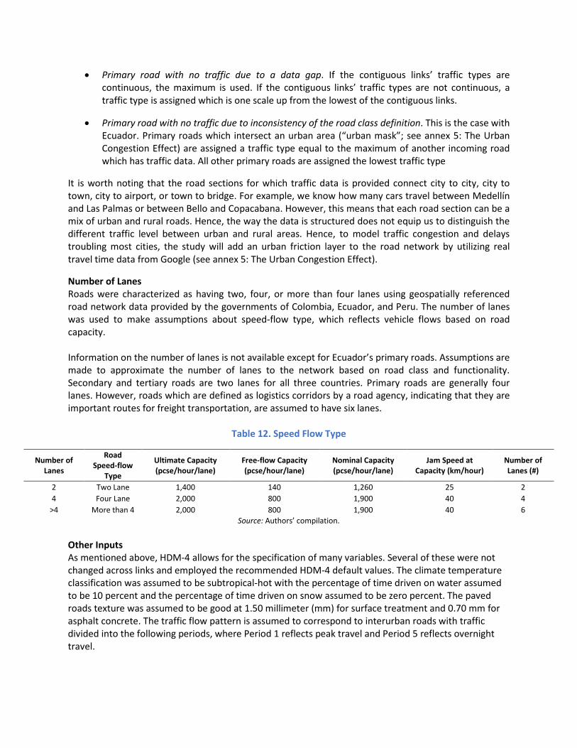
• Primary road with no traffic due to a data gap. If the contiguous links’ traffic types are continuous, the maximum is used. If the contiguous links’ traffic types are not continuous, a traffic type is assigned which is one scale up from the lowest of the contiguous links.

• Primary road with no traffic due to inconsistency of the road class definition. This is the case with Ecuador. Primary roads which intersect an urban area (“urban mask”; see annex 5: The Urban Congestion Effect) are assigned a traffic type equal to the maximum of another incoming road which has traffic data. All other primary roads are assigned the lowest traffic type

It is worth noting that the road sections for which traffic data is provided connect city to city, city to town, city to airport, or town to bridge. For example, we know how many cars travel between Medellín and Las Palmas or between Bello and Copacabana. However, this means that each road section can be a mix of urban and rural roads. Hence, the way the data is structured does not equip us to distinguish the different traffic level between urban and rural areas. Hence, to model traffic congestion and delays troubling most cities, the study will add an urban friction layer to the road network by utilizing real travel time data from Google (see annex 5: The Urban Congestion Effect).

Number of Lanes Roads were characterized as having two, four, or more than four lanes using geospatially referenced road network data provided by the governments of Colombia, Ecuador, and Peru. The number of lanes was used to make assumptions about speed-flow type, which reflects vehicle flows based on road capacity. Information on the number of lanes is not available except for Ecuador’s primary roads. Assumptions are made to approximate the number of lanes to the network based on road class and functionality. Secondary and tertiary roads are two lanes for all three countries. Primary roads are generally four lanes. However, roads which are defined as logistics corridors by a road agency, indicating that they are important routes for freight transportation, are assumed to have six lanes.

Table 12. Speed Flow Type

Number of Lanes

Road Speed-flow

Type

Ultimate Capacity (pcse/hour/lane)

Free-flow Capacity (pcse/hour/lane)

Nominal Capacity (pcse/hour/lane)

Jam Speed at Capacity (km/hour)

Number of Lanes (#)

2 Two Lane 1,400 140 1,260 25 2 4 Four Lane 2,000 800 1,900 40 4

>4 More than 4 2,000 800 1,900 40 6 Source: Authors’ compilation.

Other Inputs As mentioned above, HDM-4 allows for the specification of many variables. Several of these were not changed across links and employed the recommended HDM-4 default values. The climate temperature classification was assumed to be subtropical-hot with the percentage of time driven on water assumed to be 10 percent and the percentage of time driven on snow assumed to be zero percent. The paved roads texture was assumed to be good at 1.50 millimeter (mm) for surface treatment and 0.70 mm for asphalt concrete. The traffic flow pattern is assumed to correspond to interurban roads with traffic divided into the following periods, where Period 1 reflects peak travel and Period 5 reflects overnight travel.

Table 13. Traffic Flow Patterns (Percentage Of Annual Traffic on Each Period)

Period 1 (%) Period 2 (%) Period 3 (%) Period 4 (%) Period 5 (%) 2.17 7.59 11.64 40.24 38.36


Table 14. Number of Hours Per Year on Each Period

Period 1 (#) Period 2 (#) Period 3 (#) Period 4 (#) Period 5 (#) 87.6 350.4 613.2 2,978.4 4,730.4


The desired speed adjustment factor was set at 1 (so input speed was left unadjusted). Acceleration effects were not included in the model. The operating speed adjustment factor was set at 1 (so operating speed was left unadjusted). Finally, emissions costs and road safety costs were not included in the model. Vehicle Fleet Data Vehicle fleet data was gathered for each of the three countries included in the analysis. Data was collected for a heavy truck, and all calculations of road user costs are for this type of vehicle. The calibration parameters are set at the recommended HDM-4 default values, which reflect a modern technology vehicle fleet.

Table 15. Vehicle Fleet Data Financial Unit Costs (Heavy Truck) Colombia Ecuador Peru

50. Used vehicle cost ($/vehicle) 103,500 110,000 103,500 51. New tire cost ($/tire) 300 250 391 52. Fuel cost ($/liter) * 1.18 0.29 1.41

53. Lubricant cost ($/liter) 4.50 2.3 6.38 54. Maintenance labor cost ($/hour) 4.38 8.0 2.59

55. Crew cost ($/hour) 3.65 6.5 2.59 56. Overhead ($/year) 600 500 500 57. Interest rate (%) 12 12 12

58. Working passenger time ($/hour) 1.35 0.82 0.73 59. Nonworking passenger time ($/hour) 0.34 0.21 0.18

60. Cargo delay ($/hour) 0.100 0.09 0.09 61. Kilometers driven per year (km) 90,000 80,000 100,000

62. Hours driven per year (hr) 2,300 2,300 2,400 63. Service life (years) 10 10 10

64. Percent private use (%) 0 0 0 65. Number of passengers (#) 1 1 1

66. Work related passenger-trips (%) 0 0 0 67. Gross vehicle weight (tons) 25 25 25


Outputs

118

Road User Costs (RUCs) The output of the HDM-4 model is the unit cost of using a road expressed in dollars per vehicle-kilometer. The RUCs consist of two components: vehicle operating costs (VOCs), which reflect the cost of operating a vehicle, and value of time costs (VOTs), which reflect the cost time associated with using a vehicle. The VOCs include the cost of fuel, lubricants, tires, maintenance parts and maintenance labor, crew time, depreciation, interest, and overhead. The VOTs include the cost of passenger time and the cost of cargo time. Each of these components is calculated as an output of the HDM-4 model. Speed Beyond road user costs, HDM-4 also calculates the predicted vehicle speed in kilometers per hour for a given road link. Running the Model Stata (v.12) was used to generate the inputs for the HDM-4 model which was run iteratively for each combination of the six road characteristics in Excel using a macro designed specifically for this purpose.

119

D) Annex 4: Regression Results for Baseline Road User Costs

The mean baseline costs associated with each characteristic provide a sense of how each characteristic impacts road user costs. Two important caveats are in order. First, comparison across countries reflects the vehicle fleet data: across countries, only this vehicle fleet data (and no other characteristics) varies. Second, the length of road links is not reflected in the baseline costs: the average RUCs in a given country reflect unit, not actual, costs of using a given road. Baseline RUCs are highest in Peru at $1.70 per vehicle-km and lowest in Ecuador at $1.25 per vehicle-km (figure 6). Fuel and parts, and to a lesser extent depreciation, drive RUCs in Peru and Colombia. In Ecuador, where fuel is significantly subsidized, road user costs are driven by parts with fuel, maintenance labor, crew time, and depreciation all representing between 10 and 14 percent of total unit costs (table 16). The mean speed for each country is 51.92 km/hour and the median is 46.08 km/hour. Speed does not vary across countries; that is, speed varies across road characteristics but not across vehicle fleet characteristics.

Figure 6. Baseline Road User Costs in Colombia, Ecuador, and Peru


$1.60

$1.25

$1.70

$-

$0.20

$0.40

$0.60

$0.80

$1.00

$1.20

$1.40

$1.60

$1.80


RUCs

($/v

ehic

le-k

m)

120

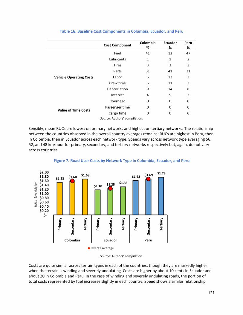
Table 16. Baseline Cost Components in Colombia, Ecuador, and Peru

Cost Component Colombia %

Ecuador %

Peru %

Vehicle Operating Costs

Fuel 41 13 47 Lubricants 1 1 2

Tires 3 3 3 Parts 31 41 31 Labor 5 12 3

Crew time 5 11 3 Depreciation 9 14 8

Interest 4 5 3 Overhead 0 0 0

Value of Time Costs Passenger time 0 0 0

Cargo time 0 0 0 Source: Authors’ compilation.

Sensibly, mean RUCs are lowest on primary networks and highest on tertiary networks. The relationship between the countries observed in the overall country averages remains: RUCs are highest in Peru, then in Colombia, then in Ecuador across each network type. Speeds vary across network type averaging 56, 52, and 48 km/hour for primary, secondary, and tertiary networks respectively but, again, do not vary across countries.

Figure 7. Road User Costs by Network Type in Colombia, Ecuador, and Peru


Costs are quite similar across terrain types in each of the countries, though they are markedly higher when the terrain is winding and severely undulating. Costs are higher by about 10 cents in Ecuador and about 20 in Colombia and Peru. In the case of winding and severely undulating roads, the portion of total costs represented by fuel increases slightly in each country. Speed shows a similar relationship

$1.53 $1.60 $1.68

$1.18 $1.25 $1.33

$1.62 $1.69 $1.78

$- $0.20 $0.40 $0.60 $0.80 $1.00 $1.20 $1.40 $1.60 $1.80 $2.00

Prim

ary

Seco

ndar

y

Tert

iary

Prim

ary

Seco

ndar

y

Tert

iary

Prim

ary

Seco

ndar

y

Tert

iary


RUCs

($/v

ehic

le-k

m)

Overall Average

121

across terrain types, with the most severe reductions in speed occurring on winding and severely undulating surfaces.

Figure 8. Road User Costs by Terrain Type in Colombia, Ecuador, and Peru


Figure 9. Speed by Terrain Type in Colombia, Ecuador, and Peru


Costs vary substantially depending on whether a road is paved or unpaved: in each country, unpaved roads are at least 50 cents more costly than paved ones. The portion of total costs composed by fuel declines slightly from paved to unpaved roads while that composed by maintenance for parts increases somewhat. Speed is similarly affected: predicted vehicle speed on paved roads is 64 km/hour while on unpaved roads it is only 40 km/hour.

$-

$0.50

$1.00

$1.50

$2.00

$2.50

Straightand level

Mostlystraight

and gentlyundulating

Bendy andgenerally

level

Bendy andgently

undulating

Bendy andseverely

undulating


Windingand

severelyundulating

Road

use

r cos

ts ($

/veh

icle

-km

)


55 55 55 54 52 49

45

0

10

20

30

40

50

60

Straightand level

Mostlystraight

and gentlyundulating

Bendy andgenerally

level

Bendy andgently

undulating

Bendy andseverely

undulating


Windingand

severelyundulating

Spee

d (k

m/h

our)

Overall Average

122

Figure 70. Road Costs by Surface Type in Colombia, Ecuador, and Peru


Costs also significantly increase as road condition declines: roads in poor condition are more than 20 cents more costly than roads in good condition in each country. Again, the composition of total costs shifts somewhat from fuel to maintenance for parts in each country. Speed declines dramatically between roads in fair and poor condition: predicted vehicle speed on a road in good condition is 59 km/hour and 54 km/hour on a road in fair condition but only 43 km/hour on a road in poor condition. Traffic, however, has almost no impact on cost: costs are the same across all traffic levels in all three countries, with a very small increase in the less than 10,000 AADT category in Colombia and Ecuador. Similarly, predicted vehicle speed only declines slightly with traffic level. Finally, costs decline slightly with the number of lanes, but only when shifting from two lanes to four lanes. Conversely, speed increases slightly when moving from two lanes to four lanes.

$1.29

$1.92

$0.99

$1.51

$1.37

$2.02

$-

$0.50

$1.00

$1.50

$2.00

$2.50

Paved Unpaved Paved Unpaved Paved Unpaved


Road

Use

r Cos

t ($/

vehi

cle-

km)

Overall Average

123

Figure 81. Road User Costs by Road Condition in Colombia, Ecuador, and Peru


Figure 92. Road User Costs by Traffic Level in Colombia, Ecuador, and Peru


$1.40 $1.59

$1.81

$1.06 $1.24

$1.46 $1.49 $1.69

$1.91

$-

$0.50

$1.00

$1.50

$2.00

$2.50



Road

Use

r Cos

t ($/

vehi

cle-

km)

Overall Average

$- $0.20 $0.40 $0.60 $0.80 $1.00 $1.20 $1.40 $1.60 $1.80

Road

Use

r Cos

t ($/

vehi

cle-

km)


124

Figure 103. Road User Costs by Number Of Lanes in Colombia, Ecuador, and Peru


The standard deviation of costs and speeds within each characteristic shows for which characteristics road user costs and speeds vary most (table 17). Costs vary most with surface type and road condition and least with traffic level, lanes, network type, and surface type.

Table 167. Standard Deviation of Road User Costs and Speed by Characteristic

Colombia Ecuador Peru Speed Network type 0.064 0.061 0.065 2.959 Terrain type 0.077 0.033 0.091 3.617 Surface type 0.311 0.260 0.324 11.799

Road condition 0.167 0.163 0.169 6.762 Traffic level 0.000 0.000 0.000 0.100

Lanes 0.014 0.014 0.013 1.582 Source: Authors’ compilation.

The highest-cost combination of characteristics for all three countries is an unpaved, tertiary, two-lane road in poor condition which is winding and severely undulating and has a traffic level of less than 10,000 AADT. The unit cost of using this road is $2.48 per vehicle-km in Colombia, $1.96 per vehicle-km in Ecuador, and $2.62 per vehicle-km in Peru. The lowest-cost combination of characteristics in Colombia and Peru is a paved, secondary, two-lane road in good condition which is straight and level and has a traffic level of less than 10,000 AADT. The unit cost of this type of road is $1.07 per vehicle-km in Colombia and $1.14 per vehicle-km in Peru. In Ecuador, there are several combinations of least-cost roads: all are paved, primary roads in good condition which are straight and level. Only traffic levels 3,000 to 6,000 and 6,000 to 10,000 on two-lane roads are not least-cost combinations. The unit cost of this type of road is $0.77 per vehicle-km.

$1.62 $1.59 $1.59

$1.27 $1.24 $1.24

$1.71 $1.69 $1.69

$-

$0.20

$0.40

$0.60

$0.80

$1.00

$1.20

$1.40

$1.60

$1.80

2 lanes 4 lanes >4 lanes 2 lanes 4 lanes >4 lanes 2 lanes 4 lanes >4 lanes


Road

use

r cos

t ($/

vehi

cle-

km)

Overall Average

125

The highest predicted vehicle speed is 86.76 km/hour and occurs on a paved, primary road in good condition which is straight and level. Only traffic levels 3,000 to 6,000, 6,000 to 10,000, and more than 10,000 AADT on two-lane roads are not speed-maximizing combinations. The minimum predicted vehicle speed is 25 km/hour and occurs on an unpaved, tertiary, two-lane road with traffic levels of either 6,000 to 10,000 or more than 10,000 AADT. Any terrain type in combination with these elements is a lowest-speed combination. A simple country-specific OLS regression of road characteristics on RUCs provides more evidence of which characteristics are influencing unit RUCs in the HDM-4 model (See table 18). Moving from a paved to an unpaved road increases RUCs more than $0.50 per vehicle-km in all three countries while moving from good to poor condition increases RUCs around $0.40 per vehicle-km. A winding and severely undulating road is between $0.10 and $0.20 more expensive per vehicle-km than a straight and level road. Network type3 and number of lanes have a smaller impact and traffic levels do not have a statistically significant impact. The same type of OLS regression was repeated with predicted vehicle speed as the dependent variable (See table 19). Similar results are obtained. Moving from a paved to an unpaved road decreases speed more than 20 km/hour and moving from good to poor condition decreases speed 16 km/hour. Terrain type also has a substantial impact: a winding and severely undulating road results in speeds which are 10 km/hour lower than a straight and level road. Moving from a primary to a tertiary network reduces speed by 7 km/hour while increasing the number of lanes increases speeds by 3 km/hour. Traffic levels do not have a statistically significant effect. The R2 is slightly lower in the case of predicted vehicle speeds than it was in the case of RUCs.

3 Note that network type and road surface type are used to make assumptions about road condition, in part explaining why network type itself has less of an impact.

126

Table 18. OLS Regression of Baseline RUCs on Road Characteristics in Colombia, Ecuador, and Peru

Colombia Ecuador Peru Secondary network 0.0735*** 0.0706*** 0.0743***

(0.00341) (0.00221) (0.00382) Tertiary network 0.156*** 0.149*** 0.158***

(0.00341) (0.00221) (0.00382) Unpaved 0.622*** 0.520*** 0.648***

(0.00279) (0.00180) (0.00312) Fair condition 0.189*** 0.173*** 0.194***

(0.00341) (0.00221) (0.00382) Poor condition 0.410*** 0.397*** 0.413***

(0.00341) (0.00221) (0.00382) 300–1,000 -0 -0 -0

(0.00483) (0.00313) (0.00540) 1,000–3,000 -0 -0 -0

(0.00483) (0.00313) (0.00540) 3,000–6,000 0.000117 0.000202 8.46e-05

(0.00483) (0.00313) (0.00540) 6,000–10,000 0.000723 0.00123 0.000529

(0.00483) (0.00313) (0.00540) >10,000 0.00183 0.00297 0.00141

(0.00483) (0.00313) (0.00540) 4 lanes -0.0294*** -0.0292*** -0.0276***

(0.00341) (0.00221) (0.00382) >4 lanes -0.0294*** -0.0292*** -0.0276***

(0.00341) (0.00221) (0.00382) Mostly straight and gently undulating 0.00469 0.00271 0.00579

(0.00521) (0.00338) (0.00583) Bendy and generally level 0.000780 0.000431 0.000903

(0.00521) (0.00338) (0.00583) Bendy and gently undulating 0.0114** 0.00678** 0.0139**

(0.00521) (0.00338) (0.00583) Bendy and severely undulating 0.0465*** 0.0244*** 0.0556***

(0.00521) (0.00338) (0.00583) Winding and gently undulating 0.0400*** 0.0252*** 0.0453***

(0.00521) (0.00338) (0.00583) Winding and severely undulating 0.232*** 0.101*** 0.274***

(0.00521) (0.00338) (0.00583) Constant 0.988*** 0.725*** 1.053***

(0.00607) (0.00393) (0.00680) Observations 2,268 2,268 2,268

R-squared 0.969 0.982 0.964 Source: Authors’ compilation.

Note: Standard errors in parentheses. *** p<0.01, ** p<0.05, * p<0.1.

127

Table 179. OLS Regression of Baseline Predicted Vehicle Speeds on Road Characteristics in Colombia, Ecuador, and Peru

Colombia Ecuador Peru Secondary network -3.708*** -3.708*** -3.708***

(0.342) (0.342) (0.342) Tertiary network -7.248*** -7.248*** -7.248***

(0.342) (0.342) (0.342) Unpaved -23.60*** -23.60*** -23.60***

(0.279) (0.279) (0.279) Fair condition -4.765*** -4.765*** -4.765***

(0.342) (0.342) (0.342) Poor condition -16.12*** -16.12*** -16.12***

(0.342) (0.342) (0.342) 300–1,000 0 0 0

(0.484) (0.484) (0.484) 1,000–3,000 0 0 0

(0.484) (0.484) (0.484) 3,000–6,000 -0.0415 -0.0415 -0.0415

(0.484) (0.484) (0.484) 6,000–10,000 -0.258 -0.258 -0.258

(0.484) (0.484) (0.484) >10,000 -0.602 -0.602 -0.602

(0.484) (0.484) (0.484) 4 lanes 3.356*** 3.356*** 3.356***

(0.342) (0.342) (0.342) >4 lanes 3.356*** 3.356*** 3.356***

(0.342) (0.342) (0.342) Mostly straight and gently undulating -0.148 -0.148 -0.148

(0.522) (0.522) (0.522) Bendy and generally level -0.113 -0.113 -0.113

(0.522) (0.522) (0.522) Bendy and gently undulating -0.702 -0.702 -0.702

(0.522) (0.522) (0.522) Bendy and severely undulating -3.054*** -3.054*** -3.054***

(0.522) (0.522) (0.522) Winding and gently undulating -5.989*** -5.989*** -5.989***

(0.522) (0.522) (0.522) Winding and severely undulating -10.21*** -10.21*** -10.21***

(0.522) (0.522) (0.522) Constant 75.13*** 75.13*** 75.13***

(0.608) (0.608) (0.608) Observations 2,268 2,268 2,268

R-squared 0.827 0.827 0.827

128

Source: Authors’ compilation. Note: Standard errors in parentheses. *** p<0.01, ** p<0.05, * p<0.1.

Table 2018. OLS Regression of RUCs on Road Characteristics in Colombia, Ecuador, and Peru

Colombia Ecuador Peru Secondary network 0.239*** 0.168*** 0.0187***

(0.00318) (0.000885) (0.00249) Tertiary network 0.359*** 0.296*** 0.106***

(0.00270) (0.000853) (0.00228) Unpaved 0.481*** 0.423*** 0.785***

(0.00260) (0.000528) (0.000704) Fair condition 0.145*** 0.197*** 0.153***

(0.00231) (0.000656) (0.000870) Poor condition 0.343*** 0.477*** 0.453***

(0.00438) (0.000833) (0.000970) 300–1,000 -0.000906 0.00161 -0.0102***

(0.00235) (0.00106) (0.00267) 1,000–3,000 0.0122*** -0.00132 0.00830***

(0.00216) (0.000879) (0.00322) 3,000–6,000 0.0130*** 0.00571*** -0.00665

(0.00246) (0.000885) (0.00423) 6,000–10,000 0.0164*** 0.0124*** 0.00943**

(0.00289) (0.00104) (0.00399) >10,000 0.0240*** 0.0154*** 0.0530***

(0.00299) (0.000927) (0.0118) 4 lanes 0.00376***

(0.000837) >4 lanes 0.0226*** 0.0475***

(0.00188) (0.00219) Mostly straight and gently undulating -0.00883*** 0.00187 0.00680***

(0.00316) (0.00229) (0.00177) Bendy and generally level -0.00865** -0.00126 -0.00260

(0.00404) (0.00241) (0.00253) Bendy and gently undulating -0.00721** 0.00540** 0.0168***

(0.00324) (0.00241) (0.00179) Bendy and severely undulating 0.0156*** 0.0197*** 0.0509***

(0.00315) (0.00230) (0.00173) Winding and gently undulating 0.00799** 0.0173*** 0.0483***

(0.00380) (0.00283) (0.00200) Winding and severely undulating 0.148*** 0.0877*** 0.214***

(0.00350) (0.00280) (0.00175) Constant 1.106*** 0.753*** 1.098***

(0.00366) (0.00244) (0.00281) Observations 8,580 34,494 49,712



129

Table 191. OLS Regression of Speed on Road Characteristics in Colombia, Ecuador, and Peru

Colombia Ecuador Peru Secondary network -11.56*** -8.553*** -3.649***

(0.660) (0.156) (0.248) Tertiary network -14.00*** -12.34*** -7.258***

(0.560) (0.151) (0.228) Unpaved -20.32*** -26.06*** -28.58***

(0.540) (0.0933) (0.0703) Fair condition -4.608*** -13.24*** -4.492***

(0.478) (0.116) (0.0869) Poor condition -14.81*** -22.62*** -12.52***

(0.909) (0.147) (0.0968) 300–1,000 1.745*** -1.139*** -0.160

(0.488) (0.188) (0.267) 1,000–3,000 -0.981** -0.958*** 0.340

(0.448) (0.156) (0.321) 3,000–6,000 -2.856*** -1.836*** -1.979***

(0.510) (0.157) (0.422) 6,000–10,000 -7.888*** -3.960*** -2.194***

(0.600) (0.184) (0.398) >10,000 -9.379*** -8.040*** -5.140***

(0.620) (0.164) (1.177) 4 lanes -0.122

(0.148) >4 lanes -6.652*** 0.846***

(0.332) (0.219) Mostly straight and gently undulating 1.890*** -1.641*** -0.254

(0.656) (0.406) (0.177) Bendy and generally level 2.747*** -1.053** -0.166

(0.838) (0.427) (0.253) Bendy and gently undulating 2.015*** -2.744*** -0.654***

(0.672) (0.426) (0.179) Bendy and severely undulating 0.330 -4.937*** -1.520***

(0.654) (0.408) (0.173) Winding and gently undulating -0.0622 -4.529*** -4.770***

(0.789) (0.500) (0.200) Winding and severely undulating -2.721*** -9.480*** -6.487***

(0.726) (0.496) (0.174) Constant 68.13*** 84.42*** 75.03***

(0.759) (0.431) (0.280) Observations 8,580 34,494 49,712



130

E) Annex 5: The Urban Congestion Effect

Due to higher traffic, urban center tends to suffer from congestion problems (or higher friction in the urban center in GIS terms). The average speeds of vehicles in the city are expected to be lower than rural areas assuming all other conditions are equal. With this additional information, one can model the increased road user cost in the urban centers when conducting the network routing simulation. An urban cluster mask is created and road links that fall within the mask are given a travel time and speeds based on Google’ algorithm to illustrate such congestion effect.

The urban cluster mask is defined based on three criteria: 1) percentage of built-up land within a given area is greater than zero, 2) population is greater than 25,000, and 3) all national and provincial capitals are represented. Two spatial datasets, built-up area global reference layer (built-up land density in 1 sq km [km2] pixel) and Landscan (population headcounts in 1 km2 pixel), are used for the calculation. The first criterion allows capturing all the developed lands, on which there is the presence of physical constructs. The population threshold and administrative status ensure one includes all the populated places and geopolitically important cities. Once the urban cluster mask is delineated, they are geocoded with the name of a corresponding city or town.

Roads that intersect the urban cluster mask are identified and considered as the subjects of the urban friction analysis. In the case where roads extend beyond 1 km buffer of the mask, they are segmented based on the extent of the buffered mask.

For each urban road link, the average speed and travel time of the GIS road network and that derived from Google’s underlying road data and algorithm can be compared and assessed. An initial assessment of Google’s travel time algorithm indicates there is a noticeable distinction in the average travel time between an urban area and nonurban. Hence, theoretically, a reduction in the average speeds from Google’s results should be expected, especially knowing that the speed of our road links, an output of the HDM4 model, is not affected by traffic.

Figure 114. Scatterplot of Google Travel Time vs GIS Travel Time a. Colombia b. Ecuador c. Peru


0

1

2

3

4

5

-0.1 0.1 0.3 0.5

GIS

Trav

el ti

me

(hr)

Google Travel time (hr)

0

0.1

0.2

0.3

0.4

0.5

-0.1 0.1 0.3 0.5

GIS

Tra

vel T

ime

(hr)

Google Travel Tme (hr)

0

0.1

0.2

0.3

0.4

0.5

-0.1 0.1 0.3 0.5

GIS

Tra

vel T

ime

(hr)

Google Travel Time (hr)

131

According to the scatterplots, travel time based on Google’s algorithm is generally higher than that in the GIS road network (that is, more data points beneath the diagonal line). However, it is noticeable that there are many cases where Google travel time is zero or lower.

Since one expects Google travel time to be greater (or lower average speeds) due to the fact its algorithm captures congestion in the urban areas, the following calibration steps were taken to ensure that, for all urban links, the newly adjusted speeds are lower than the HDM4 speeds.

1. For road links where Google speeds are lower than the HDM4 speeds, Google speeds are applied to replace the HDM4 speeds and a coefficient (ratio of Google speeds over HDM4 speeds) is computed for each link

2. Urban links where Google Direction Application Program Interface (API) does not resolve a travel time are excluded from the calculation

3. Urban links whose distance is less than 100 meter are excluded from the calculation 4. Urban links whose length is 20 percent more or less than the driving distance according to

Google are excluded from the calculation 5. The links that are previously dropped from the calculation will be assigned with the average

ratio associated to the city, in which they reside 6. The newly adjusted speeds for these links are calibrated based on their original HDM4 speeds

and city-level ratio

The urban friction coefficient is defined as the following:

𝑈𝑈𝑈𝑈𝑈𝑈𝑈𝑈𝑈𝑈 𝐹𝐹𝑈𝑈𝐹𝐹𝐹𝐹𝐹𝐹𝐹𝐹𝐹𝐹𝑈𝑈 𝐶𝐶𝐹𝐹𝐶𝐶𝐶𝐶𝐶𝐶𝐹𝐹𝐹𝐹𝐹𝐹𝐶𝐶𝑈𝑈𝐹𝐹𝑖𝑖 = 1 − 𝐺𝐺𝐹𝐹𝐹𝐹𝐺𝐺𝐺𝐺𝐶𝐶 𝑆𝑆𝑆𝑆𝐶𝐶𝐶𝐶𝑆𝑆𝑆𝑆𝑖𝑖

𝑂𝑂𝑈𝑈𝐹𝐹𝐺𝐺𝐹𝐹𝑈𝑈𝑈𝑈𝐺𝐺 𝐻𝐻𝐻𝐻𝐻𝐻4 𝑆𝑆𝑆𝑆𝐶𝐶𝐶𝐶𝑆𝑆𝑆𝑆𝑖𝑖

For any urban road link i, where Google speed is lower.

Thus, the urban friction coefficient should be interpreted as a percentage speed reduction of the original HDM4 speed estimates. For the urban road links in Colombia, Ecuador, and Peru, the average friction coefficients are 0.50, 0.36, and 0.39 respectively. In other words, there is on average a 50 percent speed reduction in Colombia, 36 percent speed reduction in Ecuador, and 39 percent speed reduction in Peru in the urban centers defined by the study.

It is safe to presume that highly populated cities are more likely to have congestion problems. Therefore, one quick way to validate the calculated urban friction coefficient is too see if it has any correlation with population density. The friction coefficient is aggregated for each urban cluster and regressed against population density. The results suggest that the correlation is positive and statistically significant, at least for Colombia and Ecuador.

132

Table 202. Regression Table, City-level Friction Coefficient and Population Density

Urban Friction Coefficient


Population density 0.00000404* 0.0000129* 0.00000264

(1.6666) (2.999) (0.7431)

Constant 0.4777*** 0.3117*** 0.3623***

(30.9149) (14.552) (14.455)

Observation 120 45 59

Source: Authors’ compilation. Note: t-statistics in parenthesis; *p<0.1, **p,0.05, ***p<0.001.

133

F) Annex 6: Road User Costs by Characteristics in Colombia, Ecuador, and Peru

Table 213. Road User Costs Characteristics

Colombia

Paved: 2 Lanes

Good Fair Poor

Traffic ('00s) <3 3–10 10–30 30–60 60–100 >100 <3 3–10 10–30 30–60 60–

100 >100 <3 3–10 10–30 30–60 60–100 >100

Primary

Bendy and generally level 1.09 1.09 1.09 1.09 1.09 1.08 1.19 1.19 1.19 1.19 1.19 1.18 1.35 1.35 1.35 1.35 1.35 1.35

Bendy and gently undulating 1.10 1.10 1.10 1.10 1.09 1.08 1.20 1.20 1.20 1.20 1.19 1.18 1.36 1.36 1.36 1.36 1.36 1.36

Bendy and severely undulating 1.12 1.12 1.12 1.12 1.12 1.12 1.22 1.22 1.22 1.22 1.21 1.21 1.43 1.43 1.43 1.43 1.43 1.44

Mostly straight and gently undulating 1.09 1.09 1.09 1.09 1.09 1.08 1.19 1.19 1.19 1.19 1.19 1.18 1.35 1.35 1.35 1.35 1.35 1.36

Straight and level 1.09 1.09 1.09 1.09 1.09 1.08 1.19 1.19 1.19 1.19 1.19 1.18 1.35 1.35 1.35 1.35 1.35 1.35

Winding and gently undulating 1.12 1.12 1.12 1.12 1.12 1.11 1.23 1.23 1.23 1.22 1.22 1.21 1.41 1.41 1.41 1.41 1.41 1.41

Winding and severely undulating 1.36 1.36 1.36 1.36 1.36 1.36 1.46 1.46 1.46 1.46 1.46 1.45 1.66 1.66 1.66 1.66 1.66 1.66

Secondary








Tertiary






134



Paved: 4 Lanes

Good Fair Poor

Traffic ('00s) <3 3–10 10–30 30–60 60–100 >100 <3 3–10 10–30 30–60 60–

100 >100 <3 3–10 10–30 30–60 60–100 >100

Primary








Secondary








Tertiary








135

Paved: 6 Lanes

Good Fair Poor

Traffic ('00s) <3 3–10 10–30 30–60 60–100 >100 <3 3–10 10–30 30–60 60–

100 >100 <3 3–10 10–30 30–60 60–100 >100

Primary








Secondary








Tertiary








Unpaved: 2 Lanes

Good Fair Poor

136

Traffic ('00s) <3 3–10 10–30 30–60 60–100 >100 <3 3–10 10–30 30–60 60–

100 >100 <3 3–10 10–30 30–60 60–100 >100

Primary








Secondary








Tertiary








Unpaved: 4 Lanes

Good Fair Poor

Traffic ('00s) <3 3–10 10–30 30–60 60–100 >100 <3 3–10 10–30 30–60 60–

100 >100 <3 3–10 10–30 30–60 60–100 >100

Primary

137








Secondary








Tertiary








Unpaved: 6 Lanes

Good Fair Poor

Traffic ('00s) <3 3–10 10–30 30–60 60–100 >100 <3 3–10 10–30 30–60 60–

100 >100 <3 3–10 10–30 30–60 60–100 >100

Primary




138





Secondary








Tertiary








Ecuador

Paved: 2 Lanes

Good Fair Poor

Traffic ('00s) <3 3–10 10–30 30–60 60–100 >100 <3 3–10 10–30 30–60 60–

100 >100 <3 3–10 10–30 30–60 60–100 >100

Primary






139



Secondary








Tertiary








Paved: 4 Lanes

Good Fair Poor

Traffic ('00s) <3 3–10 10–30 30–60 60–100 >100 <3 3–10 10–30 30–60 60–

100 >100 <3 3–10 10–30 30–60 60–100 >100

Primary








140

Secondary








Tertiary








Paved: 6 Lanes

Good Fair Poor

Traffic ('00s) <3 3–10 10–30 30–60 60–100 >100 <3 3–10 10–30 30–60 60–

100 >100 <3 3–10 10–30 30–60 60–100 >100

Primary








Secondary


141







Tertiary








Unpaved: 2 Lanes

Good Fair Poor

Traffic ('00s) <3 3–10 10–30 30–60 60–100 >100 <3 3–10 10–30 30–60 60–

100 >100 <3 3–10 10–30 30–60 60–100 >100

Primary








Secondary





142




Tertiary








Unpaved: 4 Lanes

Good Fair Poor

Traffic ('00s) <3 3–10 10–30 30–60 60–100 >100 <3 3–10 10–30 30–60 60–

100 >100 <3 3–10 10–30 30–60 60–100 >100

Primary








Secondary








143

Tertiary








Unpaved: 6 Lanes

Good Fair Poor

Traffic ('00s) <3 3–10 10–30 30–60 60–100 >100 <3 3–10 10–30 30–60 60–

100 >100 <3 3–10 10–30 30–60 60–100 >100

Primary








Secondary








Tertiary


144







Peru

Paved: 2 Lanes

Good Fair Poor

Traffic ('00s) <3 3–10 10–30 30–60 60–100 >100 <3 3–10 10–30 30–60 60–

100 >100 <3 3–10 10–30 30–60 60–100 >100

Primary








Secondary








Tertiary




145





Paved: 4 Lanes

Good Fair Poor

Traffic ('00s) <3 3–10 10–30 30–60 60–100 >100 <3 3–10 10–30 30–60 60–

100 >100 <3 3–10 10–30 30–60 60–100 >100

Primary








Secondary








Tertiary







146


Paved: 6 Lanes

Good Fair Poor

Traffic ('00s) <3 3–10 10–30 30–60 60–100 >100 <3 3–10 10–30 30–60 60–

100 >100 <3 3–10 10–30 30–60 60–100 >100

Primary








Secondary








Tertiary








Unpaved: 2 Lanes

147

Good Fair Poor

Traffic ('00s) <3 3–10 10–30 30–60 60–100 >100 <3 3–10 10–30 30–60 60–

100 >100 <3 3–10 10–30 30–60 60–100 >100

A Primary








Secondary








Tertiary








Unpaved: 4 Lanes

Good Fair Poor

Traffic ('00s) <3 3–10 10–30 30–60 60–100 >100 <3 3–10 10–30 30–60 60–

100 >100 <3 3–10 10–30 30–60 60–100 >100

148

Primary








Secondary








Tertiary








Unpaved: 6 Lanes

Good Fair Poor

Traffic ('00s) <3 3–10 10–30 30–60 60–100 >100 <3 3–10 10–30 30–60 60–

100 >100 <3 3–10 10–30 30–60 60–100 >100

Primary


149







Secondary








Tertiary









150

G) Annex 8. Alternative Estimations of Accessibility

One of the main contributions of this study is methodological. In the process of defining and selecting options for accessibility estimates, many alternatives were explored using different functional forms for the impedance or friction component of the formula as well as different weights.4 All accessibility estimates summarized here satisfy the following:

• All calculations are based on RUCs. These are estimates of the cost of using road infrastructure made using HDM-4 by considering specific attributes for each link of existing road networks such as location, class, surface type, traffic level, number of lanes, condition, and terrain type.

• Estimates are calculated over optimal (least-cost) routes connecting critical nodes. Unless otherwise noted, critical nodes are defined as national capitals, provincial capitals, population centers greater than 25,000 people, main ports, main airports, and border crossings.

• Consistent with the gravity approach, all accessibility estimates are inversely proportional to RUCs.

• Accessibility estimates are expressed as tons/$100, except where otherwise noted. This means, in practice, that broadly speaking the accessibility estimates can be interpreted as the potential economic activity (or opportunities for population mobility) unlocked by a specific transport network connecting origins with destinations. In other words, the accessibility estimates reflect the opportunities for interactions between two or more specific locations given the cost borne by the user to “move” from one location to another.

i. Infrastructure-based Accessibility: Inverse Cost

The infrastructure-based measure of accessibility imposes a functional form on the cost of travel between an origin city i and a destination city j. The functional form chose is inverse cost5: as costs increase, accessibility approaches zero. As 𝐴𝐴𝑖𝑖 increases, accessibility increases. This accessibility estimate uses the inverse of the RUC as the functional form for impedance such that �𝐹𝐹𝑖𝑖𝑖𝑖� = 1

𝑐𝑐𝑖𝑖𝑖𝑖 . Let 𝐴𝐴𝑖𝑖 represent accessibility at node i, then

Equation 1

𝐴𝐴𝑖𝑖 = ∑ � 1𝑛𝑛−1

� ∗ 𝐶𝐶(𝐹𝐹𝑖𝑖𝑖𝑖)𝑛𝑛𝑖𝑖=1;𝑖𝑖≠𝑖𝑖 = ∑ � 1

𝑛𝑛−1� ∗ � 1

𝑐𝑐𝑖𝑖𝑖𝑖)�𝑛𝑛

𝑖𝑖=1

𝐴𝐴𝑖𝑖 is accessibility measured at origin i; 𝐹𝐹𝑖𝑖𝑖𝑖 is the cost of travel between origin i and destination j; and 𝑈𝑈 is the number of all possible destinations.

4 Detailed estimates are available from authors upon request. 5 This approach follows Taylor, Sekhar, and D’Este (2006), which uses the inverse of distance as the impedance function.

152

Table 224. Infrastructure-based Accessibility: Descriptive Statistics (ton/$100)


SD 1.9 3.3 1.6 Max name Armenia Atuntaqui Peralvillo Max score 10.3 16.4 8.4

Min name Puerto Carreño

Pte De Integración Iquitos

Min score 1.2 3.5 0.9


Table 235. Infrastructure-based Accessibility: Origins with the Highest and Lowest Accessibility (ton/$100)

Colombia Ecuador

Origin Type6 Region Acc Rank Origin Type Region Acc Rank

Mos

t Ac

cess

ible

Armenia C Andina 10.3 1 Atuntaqui C Sierra 16.4 1 Calarca C Andina 9.9 2 Alfaro C Costa 15.9 2

Santa Rosa De Cabal C Andina 9.2 3 Quito C Sierra 15.4 3 El Cerrito C Andina 9.2 4 Guayaquil C Costa 15.3 4 Pereira C Andina 9.1 5 Tumbaco C Sierra 14.8 5

Leas

t Ac

cess

ible

Jorge E G Torres A Amazónica 2.5 129 Nueva Loja C Oriente 5.6 44 Arauca C Orinoquía 2.3 130 Coca C Oriente 5.5 45

La Macarena A Amazónica 2.3 131 Jose M Velasco Ibarra A Sierra 4.8 46 Tumaco C Caribe 2.2 132 Tarapoa A Oriente 4.7 47

Puerto Carreño C Orinoquía 1.2 133 Pte De Integración B Oriente 3.5 48

Peru Origin Type Region Acc Rank

Mos

t Ac

cess

ible

Peralvillo C Costa 8.4 1 Huacho C Costa 8.4 2

Lurín C Costa 8.3 3 Pachacamac C Costa 8.1 4

Lima C Costa 6.8 5

Leas

t Ac

cess

ible

Iberia A Selva 1.6 86 Desconocido B Selva 1.5 87

Alferez Vladimir Sara Bauer A Selva 1.3 88 Puerto Esperanza A Selva 1.0 89

Iquitos C Selva 0.9 90


ii. Location-based: Gravity with Population Weights

The location-based measure of accessibility maintains the functional form of the impedance function but adds a population weight to represent the opportunities available at all of the destinations accessible to origin i. These opportunities can be thought of broadly as opportunities for social interaction. The population weight used is the destination population as a share of the total population of the destinations (that is, the total population of all possible destinations excluding the origin). This measure sums the population share at each destination j divided by the cost of travel between city i and city j. As in the previous measure, as costs increase accessibility approaches zero. In contrast, the larger the population share accessible by an origin i the more accessible that origin is. As 𝐴𝐴𝑖𝑖 increases, accessibility increases.

6 “C” is city, “A” is airport, “B” is border crossing, and “P” is port.

153

Equation 2

𝐴𝐴𝑖𝑖 = ∑ 𝑃𝑃𝐹𝐹𝑆𝑆𝑆𝑆ℎ𝑈𝑈𝑈𝑈𝐶𝐶𝑖𝑖 ∙ 𝐶𝐶�𝐹𝐹𝑖𝑖𝑖𝑖�𝑛𝑛𝑖𝑖=1;𝑖𝑖≠𝑖𝑖 = ∑ 𝑃𝑃𝐹𝐹𝑆𝑆𝑆𝑆ℎ𝑈𝑈𝑈𝑈𝐶𝐶𝑖𝑖 ∙ �

1𝑐𝑐𝑖𝑖𝑖𝑖�𝑛𝑛

𝑖𝑖=1;𝑖𝑖≠𝑖𝑖

𝐴𝐴𝑖𝑖 is accessibility measured at origin i; 𝐹𝐹𝑖𝑖𝑖𝑖 is the cost of travel between origin i and destination j; 𝑃𝑃𝐹𝐹𝑆𝑆𝑆𝑆ℎ𝑈𝑈𝑈𝑈𝐶𝐶𝑖𝑖 is j’s population as a share of the total population of destinations;

and 𝑈𝑈 is the number of all possible destinations.

Table 246. Location-based Accessibility: Descriptive Statistics

(tons/$100)


SD 4.0 8.2 6.1 Max name La Pincha Alfaro Chaclacayo Max score 34.8 51.8 34.2



Min score 1.3 3.4 0.8


Table 257. Location-based Accessibility: Origins with the Highest and Lowest Accessibility (ton/$100)

Colombia Ecuador Origin Type Region Acc Rank Origin Type Region Acc Rank

Mos

t Ac

cess

ible

La Pincha C Andina 34.8 1 Alfaro C Costa 51.8 1 Chía C Andina 19.1 2 Tumbaco C Sierra 32.7 2

Facatativá C Andina 18.9 3 Daule C Costa 25.3 3 Cajicá C Andina 16.8 4 Boliche C Costa 21.8 4

Girardota C Andina 14.2 5 Tahuaico C Sierra 21.8 5

Leas

t Ac

cess

ible

La Macarena A Amazónica 2.5 129 Coca C Oriente 5.1 44 Arauca C Orinoquía 2.4 130 Nueva Loja C Oriente 5.1 45

Puerto Bolivar P Caribe 2.4 131 Jose Maria Velasco Ibarra A Sierra 4.8 46 Tumaco C Caribe 2.2 132 Tarapoa A Oriente 4.3 47



Mos

t ac

cess

ible

Chaclacayo C Costa 34.2 1 Puente Piedra C Costa 33.9 2


Callao C Costa 19.3 5

Leas

t ac

cess

ible





154

iii. Location-based: Gravity with Economic Activity Weights

The fourth measure of accessibility replaces the population weight with a proxy of economic activity to represent (economic) opportunities available at all of the destinations accessible to origin i. The proxy of economic activity used here is an index created from the brightness of lights shining from small geographical areas and summed to create a measure for each city of more than 25,000 people.7 Opportunities can then be thought of as opportunities for economic interaction. Like the population-weighted measure, this measure sums the share of economic activity at each destination j (not including economic activity at origin i) divided by the cost of travel between city i and city j. As in the previous measure, as costs increase accessibility approaches zero. The larger the economic activity accessible by an origin i, the more accessible that origin is. As 𝐴𝐴𝑖𝑖 increases, accessibility increases. Note that this measure is speculative and included only for comparison purposes: the nightlights index is a unit-less, scale-less measure which provides, in essence, a ranking of economic activity. When the nightlight index is compared to other measures, ranks are used.

Equation 3

𝐴𝐴𝑖𝑖 = ∑ 𝑁𝑁𝐹𝐹𝐺𝐺ℎ𝐺𝐺𝐹𝐹𝐺𝐺ℎ𝐹𝐹𝑆𝑆𝑆𝑆ℎ𝑈𝑈𝑈𝑈𝐶𝐶𝑖𝑖 ∙ 𝐶𝐶�𝐹𝐹𝑖𝑖𝑖𝑖�𝑛𝑛𝑖𝑖=1;𝑖𝑖≠𝑖𝑖 = ∑ 𝑁𝑁𝐹𝐹𝐺𝐺ℎ𝐹𝐹𝐺𝐺𝐹𝐹𝐺𝐺ℎ𝐹𝐹𝑆𝑆𝑆𝑆ℎ𝑈𝑈𝑈𝑈𝐶𝐶𝑖𝑖 ∙ �

1𝑐𝑐𝑖𝑖𝑖𝑖�𝑛𝑛


𝐴𝐴𝑖𝑖 is accessibility measured at origin i; 𝐹𝐹𝑖𝑖𝑖𝑖 is the cost of travel between origin i and destination j; 𝑁𝑁𝐹𝐹𝐺𝐺ℎ𝐹𝐹𝐺𝐺𝐹𝐹𝐺𝐺ℎ𝐹𝐹𝑆𝑆𝑆𝑆ℎ𝑈𝑈𝑈𝑈𝐶𝐶𝑖𝑖 is j’s economic activity as a share of the total economic

activity of destinations; and 𝑈𝑈 is the number of all possible destinations.

Table 268. Economic-Activity-based Accessibility: Descriptive Statistics

Colombia Ecuador Peru 6.5 13.5 4.8 4.4 9.5 6.7 La Pincha Alfaro Chaclacayo 39.3 58.9 38.5 Puerto Carreño Pte De Integración Iquitos 1.3 3.4 0.8


Table 27. Economic Activity-based Accessibility: Origins with the Highest and Lowest Accessibility Colombia Ecuador Origin Type Region Acc Rank Origin Type Region Acc Rank

t ac ce ssi La Pincha C Andina 39.3 1 Alfaro C Costa 58.9 1

7 The Defense Meteorological Satellite Program/Operational Linescan System (DMSP/OLS) nighttime stable light data provide a potential way to map the extent and dynamics of urban areas. DMSP flies in a sun-synchronous orbit, and the OLS (Operational Linescan System) is one of the main sensors on the DMSP satellite platform. At night, the OLS sensor can detect the lowest levels of radiation, hence, its nighttime light data are often used to study human activities, urban expansion, and economic activity. The nightlight dataset used in this analysis (2011) underwent a series of radiometric calibrations to address the saturation problem (that is, the lack of variation in the higher end) in urban centers. The radiance calibrated product is a relative measure and thus deemed to be unit-less (that is, a city which has a digital value of 400 in nightlights is not two times brighter than a city with a value of 200) (Source: NOAA).

155

Chía C Andina 21.3 2 Tumbaco C Sierra 38.7 2 Facatativá C Andina 21.1 3 Daule C Costa 27.7 3

Cajicá C Andina 18.2 4 Tahuaico C Sierra 25.0 4 Zipaquirá C Andina 14.8 5 Nono C Sierra 24.1 5

Leas

t Ac

cess

ible

Puerto Bolivar P Caribe 2.6 129 Zamora C Oriente 5.3 44 La Macarena A Amazónica 2.5 130 Nueva Loja C Oriente 5.3 45

Arauca C Orinoquía 2.4 131 Jose Maria Velasco Ibarra A Sierra 4.7 46 Tumaco C Caribe 2.0 132 Tarapoa A Oriente 4.4 47



Mos

t Ac

cess

ible




Leas

t Ac

cess

ible





iv. Location-based: Gravity with Competition

The next accessibility estimate recognizes the likely presence of competition effects between cities. The population- and economic-activity-weighted measures incorporate the opportunities accessible at the destinations reachable from some origin city i. However, the origin city i is competing with all other cities for the opportunities available in a given destination j. To reflect this competition, this measure adjusts the weight for the population at all other “competitor cities,” which are all cities which are not the origin i or the destination j.8 Specifically, the measure divides the opportunities (the supply) available at any destination j by the demand for those opportunities from all other cities which are not origin i or destination j. Population shares are again used: the “opportunities” population weight in the numerator is, as before, the population at destination j as a share of the total population of all destinations excluding i; the “competition” population weight is the population at destination z as a share of the total population of all destinations excluding origin i and destination j. The “competition” population weight is itself discounted by (the inverse of) the cost of travel between destination z and destination j. As before, the “opportunities” population weight is similarly discounted by the (inverse of) the cost of travel between origin i and destination j. As 𝐴𝐴𝑖𝑖 increases, accessibility increases.

Importantly, the competition-based measure lacks units and so is not directly comparable to the other measures (though, of course, their resulting ranks can be compared). Additionally, the accessibility score is not multiplied by 100.

Equation 4

8 The economic activity weight could easily be substituted here for the population weight as in the previous accessibility measure.

156

𝐴𝐴𝑖𝑖 = ∑ � 𝑃𝑃𝑃𝑃𝑃𝑃𝑃𝑃ℎ𝑎𝑎𝑎𝑎𝑎𝑎𝑖𝑖∑ 𝑃𝑃𝑃𝑃𝑃𝑃𝑃𝑃ℎ𝑎𝑎𝑎𝑎𝑎𝑎𝑧𝑧∙𝑓𝑓(𝑐𝑐𝑧𝑧𝑖𝑖)𝑚𝑚𝑧𝑧=1; 𝑧𝑧 ≠𝑖𝑖,𝑖𝑖

�𝑛𝑛𝑖𝑖=1;𝑖𝑖≠𝑖𝑖 ∙ 𝐶𝐶�𝐹𝐹𝑖𝑖𝑖𝑖� = ∑ � 𝑃𝑃𝑃𝑃𝑃𝑃𝑃𝑃ℎ𝑎𝑎𝑎𝑎𝑎𝑎𝑖𝑖

∑ 𝑃𝑃𝑃𝑃𝑃𝑃𝑃𝑃ℎ𝑎𝑎𝑎𝑎𝑎𝑎𝑧𝑧∙1𝑐𝑐𝑧𝑧𝑖𝑖

𝑚𝑚𝑧𝑧=1; 𝑧𝑧 ≠𝑖𝑖,𝑖𝑖

�𝑛𝑛𝑖𝑖=1;𝑖𝑖≠𝑖𝑖 ∙ 1

𝑐𝑐𝑖𝑖𝑖𝑖

𝐴𝐴𝑖𝑖 is accessibility measured at origin i; 𝑃𝑃𝐹𝐹𝑆𝑆𝑆𝑆ℎ𝑈𝑈𝑈𝑈𝐶𝐶𝑖𝑖 is j’s population as a share of the total population of

destinations; 𝑃𝑃𝐹𝐹𝑆𝑆𝑆𝑆ℎ𝑈𝑈𝑈𝑈𝐶𝐶𝑧𝑧 is j’s population as a share of the total population of

destinations; 𝐶𝐶(𝐹𝐹𝑖𝑖𝑖𝑖) is an impedance function 1

𝑐𝑐𝑖𝑖𝑖𝑖;

𝐶𝐶(𝐹𝐹𝑧𝑧𝑖𝑖) is an impedance function 1𝑐𝑐𝑧𝑧𝑖𝑖

;

𝐹𝐹𝑖𝑖𝑖𝑖 is the cost of travel between origin i and destination j; 𝐹𝐹𝑧𝑧𝑖𝑖 is the cost of travel between destination z and destination j; and 𝑈𝑈 and 𝑚𝑚 are the number of all possible destinations.

Table 30. Location-based Accessibility with Competition: Descriptive Statistics


SD 0.6 0.8 0.9

Max name La Pincha Alfaro Puente Piedra

Max score 5.9 4.8 5.3



Min score 0.2 0.3 0.2


Table 281. Location-based Accessibility with Competition: Origins with the Highest and Lowest Accessibility


Mos

t Ac

cess

ible


Facatativá C Andina 3.0 3 Guayaquil C Costa 2.0 3 Cajicá C Andina 2.6 4 Tahuaico C Sierra 1.9 4

Girardota C Andina 2.5 5 Nono C Sierra 1.8 5

Leas

t Ac

cess

ible

Puerto Bolivar P Caribe 0.5 129 Nueva Loja C Oriente 0.5 44 La Macarena A Amazónica 0.4 130 Coca C Oriente 0.5 45

Arauca C Orinoquía 0.4 131 Jose Maria Velasco Ibarra A Sierra 0.4 46 Tumaco C Caribe 0.4 132 Tarapoa A Oriente 0.4 47



Mos

t Ac

cess

ible

Puente Piedra C Costa 5.3 1 Chaclacayo C Costa 5.1 2

Callao C Costa 4.4 3 Lurín C Costa 4.0 4

Pachacamac C Costa 3.6 5

Leas

t Ac

cess

ibl

e


Alferez Vladimir Sara Bauer A Selva 0.4 88

157

Puerto Esperanza A Selva 0.3 89 Iquitos C Selva 0.2 90


v. Location-based: Gravity with a Distance-decay Function

This measure of accessibility incorporates a more complex functional form into the impedance function. As described in the literature review in the main text, the impedance function provides a sense of people’s willingness to travel between two locations and assumes that this willingness declines with distance. Very similar to the gravity-based accessibility approach, an unconstrained gravity model can be used to estimate the impact of distance (or cost) on willingness to travel. A simple gravity model is of the form:

Equation 5

𝑇𝑇𝑈𝑈𝑈𝑈𝐶𝐶𝐶𝐶𝐹𝐹𝐹𝐹𝑖𝑖𝑖𝑖 = 𝛼𝛼𝑃𝑃𝐹𝐹𝑆𝑆𝑖𝑖𝜃𝜃𝑃𝑃𝐹𝐹𝑆𝑆𝑖𝑖µ𝐹𝐹𝑖𝑖𝑖𝑖

−𝛽𝛽

𝑇𝑇𝑈𝑈𝑈𝑈𝐶𝐶𝐶𝐶𝐹𝐹𝐹𝐹𝑖𝑖𝑖𝑖 is the traffic between origin i and destination j (AADT); 𝑃𝑃𝐹𝐹𝑆𝑆𝑖𝑖𝜃𝜃 is the population of origin city i; 𝑃𝑃𝐹𝐹𝑆𝑆𝑖𝑖𝜃𝜃 is the population of destination city j; and 𝐹𝐹𝑖𝑖𝑖𝑖 is the cost of traveling between origin city i and destination city j.

β is the parameter of interest in this model, representing the desire to travel between two locations (Iacono, Krizek, and El-Geneidy 2008). β can be estimated using OLS by taking the natural logarithm:

Equation 6

ln(𝑇𝑇𝑈𝑈𝑈𝑈𝐶𝐶𝐶𝐶𝐹𝐹𝐹𝐹𝑖𝑖𝑖𝑖) = ln(𝛼𝛼) + 𝜃𝜃 ln�𝑃𝑃𝐹𝐹𝑆𝑆𝑖𝑖) + µ𝐺𝐺𝑈𝑈 (𝑃𝑃𝐹𝐹𝑆𝑆𝑖𝑖�− 𝛽𝛽ln (𝐹𝐹𝑖𝑖𝑖𝑖) However, the possibility—and reality, in most applications of the gravity model—that there are zero flows between origins and destinations means that, if these zeros represent real rather than missing data, the estimates of β will be biased. There are several approaches to dealing with zero flows, including dropping the zeros and so maintaining the log-normal model or adding a constant to the zero flows (or to all flows). Both of these approaches are not ideal. Instead, following Santos Silva and Tenreyo (2006), the Poisson pseudo-maximum likelihood estimator is used, which utilizes the dependent variable in levels rather than logs and so does not drop observations with a value of zero. In sum, rather than assume a functional form for the impedance function (for example, 1

𝑐𝑐𝑖𝑖𝑖𝑖), this

approach allows the data to speak for itself by incorporating the β parameter from the traffic gravity model into the gravity-based accessibility calculation. Origin-destination flows between provincial capitals were obtained from Colombia, Ecuador, and Peru and used to estimate country-wide βs.9

9 Ministerio de Transporte de la República de Colombia (2005). Ministerio de Transportes y Comunicaciones Provias Nacional de la República de Perú (2011). Data for Colombia were obtained using the Wayback Machine at http://www.mintransporte.gov.co/portal/page/portal/mintransporte/servicios/documentos/ANEXOS_ENCUESTA_ORIGEN_DESTINO_2003.zip. Data for Ecuador were included in the Inter-American Development Bank’s database

158

http://www.mintransporte.gov.co/portal/page/portal/mintransporte/servicios/documentos/ANEXOS_ENCUESTA_ORIGEN_DESTINO_2003.zip

http://www.mintransporte.gov.co/portal/page/portal/mintransporte/servicios/documentos/ANEXOS_ENCUESTA_ORIGEN_DESTINO_2003.zip

Because of differences in the types of trips studies and the years studied and because of missing data, these betas should only be used as very rough references. Figure 15 shows the relationship between trips and distance used to derive β. Figure 125. The Relationship between Trips between Provincial Capitals and Distance in Colombia,

Ecuador, and Peru

Source: See Footnote 10.

Note also that the units of the accessibility measure are 𝑡𝑡𝑃𝑃𝑛𝑛𝛽𝛽

$𝛽𝛽, making this measure not comparable to

the other measures except in rankings.

Equation 7

𝐴𝐴𝑖𝑖 = ∑ 𝑃𝑃𝐹𝐹𝑆𝑆𝑆𝑆ℎ𝑈𝑈𝑈𝑈𝐶𝐶𝑖𝑖 ∙ 𝐶𝐶�𝐹𝐹𝑖𝑖𝑖𝑖�𝑛𝑛𝑖𝑖=1;𝑖𝑖≠𝑖𝑖 = ∑ 𝑃𝑃𝐹𝐹𝑆𝑆𝑆𝑆ℎ𝑈𝑈𝑈𝑈𝐶𝐶𝑖𝑖 ∙ �

1

𝑐𝑐𝑖𝑖𝑖𝑖𝛽𝛽�𝑛𝑛


𝐴𝐴𝑖𝑖 is accessibility measured at origin i; 𝐹𝐹𝑖𝑖𝑖𝑖 is the cost of travel between origin i and destination j; 𝑃𝑃𝐹𝐹𝑆𝑆𝑆𝑆ℎ𝑈𝑈𝑈𝑈𝐶𝐶𝑖𝑖 is j’s population as a share of the total population of destinations; 𝛽𝛽 is an empirically estimated, country-specific parameter; and

of Ecuador’s road network. Data for Peru were obtained from annexes associated with the Ministerio de Transporte y Comunicaciones’s study and is available at https://www.mtc.gob.pe/estadisticas/estudios.html.

050

000

1000

0015

0000

2000

00Tr

ips

betw

een

Orig

in a

nd D

estin

atio

n

0 500 1000 1500 2000Distance between Origin and Destination (km)

Trips vs. Distance: Colombia

020

0000

040

0000

060

0000

080

0000

0

0 200 400 600 800 1000Distance (km)

fl_ecu_ppml lowess fl_ecu_ppml km

020

0040

0060

0080

0010

000

0 1000 2000 3000 4000Distance (km)

fl_per_p_ppml lowess fl_per_p_ppml km

159

𝑈𝑈 is the number of all possible destinations.

Table 29. Location-based Accessibility: Descriptive Statistics (tonβ/$β100)


SD 4.4 8.5 5.0 Max name La Pincha Alfaro Chaclacayo Max score 37.4 53.6 28.7

Min name Puerto Carreño Pte De Integración Iquitos

Min score 3.8 1.8 0.1


Table 30. Location-based Accessibility: Origins with the Highest and Lowest Accessibility (tonβ/$β100)


Mos

t Ac

cess

ible


Facatativá C Andina 24.9 3 Daule C Costa 21.6 3 Cajicá C Andina 22.9 4 Tahuaico C Sierra 18.1 4

Zipaquirá C Andina 19.8 5 Boliche C Costa 17.7 5

Leas

t Ac

cess

ible

La Macarena A Amazónica 6.1 129 Coca C Oriente 3.0 44 Arauca C Orinoquía 5.9 130 Nueva Loja C Oriente 3.0 45

Puerto Bolivar P Caribe 5.8 131 Jose Maria Velasco Ibarra A Sierra 2.8 46 Tumaco C Caribe 5.5 132 Tarapoa A Oriente 2.4 47



Mos

t Ac

cess

ible




Leas

t Ac

cess

ible





vi. Infrastructure-based: 100 km and 200 km Catchment Areas

Because the location-based measure is highly dependent on distance, it awards higher accessibility to smaller countries (such as Ecuador) and lower accessibility to larger countries (such as Colombia and Peru). To control for distance and emphasize the impact of infrastructure (that is, roads) on accessibility, the location-based measure was recalculated for destinations within 100 km and 200 km (as the crow flies) of each origin. To emphasize the infrastructure aspect of this measure, population weights were not included in the estimation.

Equation 8

160

𝐴𝐴𝑖𝑖 = ∑ � 1𝑛𝑛−1


𝑛𝑛−1� ∗ � 1


𝑖𝑖=1

𝐴𝐴𝑖𝑖 is accessibility measured at origin i; 𝐹𝐹𝑖𝑖𝑖𝑖 is the cost of travel between origin i and destination j where j is less than

100 km or 200 km from i; and 𝑈𝑈 is the number of all possible destinations.

Table 31. Infrastructure-based Accessibility with 100 km and 200 km Catchment Areas: Descriptive Statistics

(ton/$100) 100 km


SD 1.4 2.7 1.2 Max

name Armenia Atuntaqui Lurín

Max score 6.0 11.1 5.1

Min name Eduardo Falla Solano Jose Maria Velasco Ibarra Cuzco

Min score 0.1 0.2 0.1

200 km


SD 1.9 3.4 1.4 Max name Armenia Atuntaqui Lurín Max score 8.1 13.2 6.3 Min name La Macarena Pte De Integración Atalaya Min score 0.1 0.7 0.1


Table 325. Infrastructure-based Accessibility with 100 km and 200 km Catchment Areas: Origins with the Highest and Lowest Accessibility

(ton/$100) 100 km


Mos

t Ac

cess

ible

Armenia C Andina 6.0 1 Atuntaqui C Sierra 11.1 1 Calarca C Andina 5.4 2 Quito C Sierra 9.4 2

El Cerrito C Andina 4.9 3 Ibarra C Sierra 9.3 3 Santa Rosa De Cabal C Andina 4.7 4 Otavalo C Sierra 9.2 4

Guacari C Andina 4.7 5 Tumbaco C Sierra 8.9 5

Leas

t Ac

cess

ible

Otu A Andina 0.2 125 Nueva Loja C Oriente 1.0 42 Puerto Bolivar P Caribe 0.1 126 Tarapoa A Oriente 0.9 43

Quibdo C Pacífica 0.1 127 Coca C Oriente 0.8 44 Arauca C Orinoquía 0.1 128 Esmeraldas C Costa 0.6 45

Eduardo Falla Solano A Amazónica 0.1 129 Jose Maria Velasco Ibarra A Sierra 0.2 46

100 km


t Ac ce ssi Lurín C Costa 5.1 1

161

Pachacamac C Costa 5.0 2 Peralvillo C Costa 4.8 3 Huacho C Costa 4.8 4

Lima C Costa 3.7 5

Leas

t Ac

cess

ible

Machu Pichu Airport A Sierra 0.1 79 Huamachuco C Sierra 0.1 80 Desconocido B Selva 0.1 81

Ayacucho C Sierra 0.1 82 Cuzco C Sierra 0.1 83

200 km Colombia Ecuador Origin Type Region Acc Rank Origin Type Region Acc Rank

Mos

t Ac

cess

ible

Armenia C Andina 8.1 1 Atuntaqui C Sierra 13.2 1 Calarca C Andina 7.6 2 Alfaro C Costa 13.1 2

Santa Rosa De Cabal C Andina 6.9 3 Quito C Sierra 12.5 3 Pereira C Andina 6.9 4 Guayaquil C Costa 12.3 4

Chinchiná C Andina 6.7 5 Tumbaco C Sierra 12.0 5

Leas

t A

cces

sibl

e Puerto Bolivar P Caribe 0.4 128 Nueva Loja C Oriente 2.6 44 Tumaco C Caribe 0.3 129 Esmeraldas C Costa 2.4 45 Arauca C Orinoquía 0.2 130 Jose M V Ibarra A Sierra 1.8 46

Jorge E G Torres A Amazónica 0.1 131 Tarapoa A Oriente 1.2 47 La Macarena A Amazónica 0.1 132 Pte De Integración B Oriente 0.7 48

200 km


Mos

t Ac

cess

ible

Lurín C Costa 6.3 1 Peralvillo C Costa 6.2 2 Huacho C Costa 6.2 3

Pachacamac C Costa 6.1 4 Lima C Costa 4.7 5

Leas

t Ac

cess

ible

Cuzco C Sierra 0.2 83 Machu Pichu Airport A Sierra 0.2 84

Iberia A Selva 0.2 85 Pucallpa C Selva 0.1 86 Atalaya A Selva 0.1 87


vii. Infrastructure-based: Accessibility to Functions

The final accessibility measure is similar to the catchment area measure but focuses on important economic functions by measuring accessibility to the nearest airport, port, border crossing, and other city. This approach again in some sense controls for distance and is a way of exploring accessibility to the most important connections to external markets (ports, airports, and border crossings) and to other markets (other cities with more than 25,000 people). This measure was calculated in the same way as the infrastructure-based measure10 but with destinations restricted to the least-cost port, airport, border crossing, and other city.

Equation 9

10 Population weights were not included because the population of a port, border crossing, and airport is likely not material to its accessibility. However, weights could easily be included in this measure.

162

𝐴𝐴𝑖𝑖 = ∑ � 1𝑛𝑛−1


𝑛𝑛−1� ∗ � 1


𝑖𝑖=1

𝐴𝐴𝑖𝑖 is accessibility measured at origin i; 𝐹𝐹𝑖𝑖𝑖𝑖 is the cost of travel between origin i and destination j where j is the least-

cost port, airport, border crossing, and other city; and

𝑈𝑈 is 4 (the least-cost port, airport, border crossing, and other city).

Table 33. Accessibility to Functions: Descriptive Statistics (ton/$100)


SD 0.9 2.0 1.0 Max

name Santa Marta Machala Puesto Grau

Max score 8.6 14.4 7.4

Min name

Planeta Aica Zamora Huancavelica

Min score 4.2 5.1 3.6


Table 34. Accessibility to Functions: Origins with the Highest and Lowest Accessibility (ton/$100)


Mos

t Ac

cess

ible

Santa Marta C Caribe 8.6 1 Machala C Costa 14.4 1 Ciénaga C Caribe 8.5 2 Santa Rosa C Costa 13.8 2 Turbaco C Caribe 8.4 3 Pasaje C Costa 13.6 3

Cartagena C Caribe 8.4 4 Alfaro C Costa 13.5 4 Barranquilla C Caribe 8.4 5 Guayaquil C Costa 13.4 5

Leas

t Ac

cess

ible

Quibdo C Pacífica 5.1 116 Coca C Oriente 8.3 35 Mompós C Caribe 4.9 117 Puyo C Oriente 7.8 36

Puertp Berio C Andina 4.9 118 Otavalo C Sierra 7.7 37 Sevilla C Andina 4.9 119 Nono C Sierra 7.3 38

Planeta Aica C Caribe 4.2 120 Zamora C Oriente 5.1 39


Mos

t Ac

cess

ible

Puesto Grau C Costa 7.4 1 Tumbes C Costa 7.2 2

Lambayeque C Costa 7.1 3 Chiclayo C Costa 7.1 4

Ilo C Costa 7.0 5

Leas

t Ac

cess

ible

Cerro De Pasco C Sierra 4.1 56 Pucallpa C Selva 4.0 57

Aucayacu C Selva 3.8 58 Abancay C Sierra 3.7 59

Huancavelica C Sierra 3.6 60


163

viii. Comparison of Alternative Estimates of Accessibility

All of the measures exhibit a fair degree of correlation with the highest correlations between the rankings suggested by the infrastructure-based measures (the basic infrastructure measure and the infrastructure-based catchment area measures) and between the rankings suggested by the location-based measures (the basic location-based measure, the economic activity measure, the competition measure, and the distance decay measure). There is less correspondence across the infrastructure-based and location-based measures. (Table 38and figure 16a-d). This suggests that each type of measure is picking up a different type of accessibility. The accessibility measures with the 100 and 200 km catchment areas have substantial overlaps with the other measures in several cases, while the functional measure is very different from every other method of measurement. Though the nightlights measure is a problematic proxy for gross domestic product (GDP), it is highly correlated with the (population-weighted) location-based measure (the correlation coefficient is 0.9701, 0.9699, and 0.9783 for Colombia, Ecuador, and Peru, respectively), which could mean that population is a good stand-in for economic activity. Figure 16a shows the relationship between the two measures. However, one of the most important criticisms of the nightlights proxy is that it is only useful as a proxy of economic activity in highly industrialized countries with some degree of urbanization. In all other cases, the nightlights index might reflect population density rather than economic intensity. This introduces noise in using nightlights to estimate the GDP of countries with economies driven by low-labor industries such as mining or commodities. This is the case in Colombia, Ecuador, and Peru (and, in fact, most of Latin America).

164

Table 35. There is a Significant Amount of Consistency Across the Rankings Resulting from the Different Accessibility Measures

(correlation between rankings according to accessibility indices; * indicates statistical significance at the 1% level) Colombia

Infra Loc Night Comp Decay Infra: 100 km Loc: 100 km Infra: 200 km Loc: 200 km Infra Loc 0.8891*

Night 0.8262* 0.9701* Comp 0.8707* 0.9703* 0.9773* Decay 0.8766* 0.9930* 0.9577* 0.9479*

Infra: 100 km 0.9415* 0.7714* 0.7140* 0.7880* 0.7329* Loc: 100 km 0.5740* 0.4813* 0.4372* 0.5493* 0.4223* 0.6601*

Infra: 200 km 0.9879* 0.8727* 0.8181* 0.8609* 0.8563* 0.9519* 0.5478* Loc: 200 km 0.5295* 0.5540* 0.5563* 0.6498* 0.4845* 0.6285* 0.7496* 0.5293*

Function -0.1678 -0.3674 -0.371 -0.249 -0.414 0.0908 0.6333* -0.1857 0.6119*

Ecuador


Night 0.8752* 0.9699* Comp 0.9246* 0.9675* 0.9771* Decay 0.8882* 0.9953* 0.9732* 0.9783*

Infra: 100 km 0.9668* 0.8164* 0.8411* 0.8840* 0.8467* Loc: 100 km 0.6371* 0.6938* 0.6894* 0.7180* 0.7104* 0.5963*

Infra: 200 km 0.9884* 0.8457* 0.8680* 0.9122* 0.8680* 0.9597* 0.5902* Loc: 200 km 0.8538* 0.9161* 0.9240* 0.9292* 0.9332* 0.8652* 0.7660* 0.8218*

Function 0.1998 -0.0322 -0.188 -0.0345 -0.0165 0.3407 0.2695 0.1705 0.2341

Peru


Night 0.8464* 0.9783* Comp 0.8713* 0.9299* 0.9599* Decay 0.9129* 0.9733* 0.9717* 0.9727*

Infra: 100 km 0.8385* 0.5953* 0.5959* 0.7121* 0.7135* Loc: 100 km 0.7535* 0.6104* 0.6089* 0.7231* 0.7252* 0.8217*

Infra: 200 km 0.9238* 0.6936* 0.6902* 0.7833* 0.7890* 0.9163* 0.8050* Loc: 200 km 0.6833* 0.5530* 0.5755* 0.7033* 0.6776* 0.7990* 0.7205* 0.6878*

Function 0.5153 0.1755 0.2458 0.3832 0.2886 0.5386 0.5091 0.5857* 0.6199*

Infrastructure-based

Location-based


Unfortunately, at the time of preparing this report no other measure of GDP at the local level was available for all countries. Given this limitation, for the purpose of the accessibility analysis presented in this report only estimates using population weights were considered. The data used for population is very reliable and, with a great degree of confidence, comparable, and standardized across countries.

Finally, a decision about functional form was made in the report. Given the correlation between the accessibility rankings derived from estimates with different functional forms (the correlation coefficient is 0.9930, 0.9953, and 0.9733 between the basic infrastructure measure and the location-based measure for Colombia, Ecuador, and Peru, respectively), for practical purposes and to ensure easy interpretation and replicability, the study focuses on the simplest functional form: inverse cost with a beta of -1. It is clear from the empirical estimations, however, that introducing weights makes an enormous difference in the assessment of accessibility. Accessibility indexes with and without weights are estimated and analyzed in detail in the study. Table 38 summarizes the accessibility rank of each origin using each accessibility measure estimated.

165

Figure 136. Scatterplots of Various Accessibility Estimates

a. Location-based with Population Weight versus Location-based with Nightlights Weight

(Rank)

b. Infrastructure-based versus Location-based (Score)

c. Competition Effects versus Location-based (Rank)

d. Distance Decay versus Location-based (Rank)


Table 36. Ranking of Origins by Accessibility Measure11

11 Origins with unidentified names are omitted from these tables but are included in all of the other analyses.

020

4060

Loca

tion-

Bas

ed w

ith N

ight

light

s W

eigh

t: R

ank

0 20 40 60Location-Based with Population Weight: Rank


05

1015

20In

frast

ruct

ure-

Bas

ed: S

core

0 10 20 30 40 50Location-Based: Score


050

100

150

Loca

tion-

Bas

ed: R

ank

0 50 100 150Competition Effects: Rank


050

100

150

Loca

tion-

Bas

ed: R

ank

0 50 100 150Distance Decay: Rank


166

Colombia (n=131) Type Region Infra Loc Night Comp Decay Infra: 100 km

Loc: 100 km

Infra: 200 km

Loc: 200 km

Func

Acacías C Andina 71 35 34 46 38 75 93 74 48 90 Aguachica C Andina 87 82 82 86 75 108 74 107 101 92

Agustín Codazzi C Caribe 97 102 87 94 102 111 53 97 100 73 Ancuyá C Andina 123 118 124 116 120 98 72 121 41 69

Antonio Narino A Andina 112 105 120 97 110 87 31 103 27 NA Apartadó C Caribe 31 92 104 93 97 11 4 38 26 9

Arauca C Orinoquía 128 128 129 129 128 126 124 128 112 46 Arjona C Caribe 51 50 23 24 59 34 33 47 16 11

Armenia C Andina 1 25 32 29 26 1 44 1 76 37 Ayapel C Caribe 102 107 107 110 105 96 115 100 108 102

Baranoa C Caribe 78 46 11 16 54 63 28 73 10 8 Barbosa C Andina 50 16 30 14 20 61 24 62 14 86

Barrancabermeja C Andina 81 69 70 68 66 99 98 93 87 87 Barranquilla C Caribe 82 103 94 81 106 68 84 78 52 5

Bogota C Andina 17 53 56 17 53 28 34 22 44 72 Bucaramanga C Andina 80 76 81 83 71 93 81 94 96 57 Buenaventura C Pacífica 77 64 68 73 64 82 97 79 60 19

Buga C Andina 11 32 36 32 32 12 54 14 31 36 Cajicá C Andina 10 4 4 4 4 10 23 12 8 65

Calarca C Andina 2 12 18 19 10 2 12 2 58 38 Cali C Andina 20 60 66 54 61 20 32 23 42 25

Carepa C Andina 35 73 99 77 79 19 2 42 7 16 Carmen De Viboral C Andina 23 13 26 13 13 30 21 24 19 51

Cartagena C Caribe 61 95 75 67 101 47 87 54 54 4 Cartago C Andina 9 27 35 34 27 9 40 8 56 64 Caucasia C Caribe 84 91 91 92 86 100 85 83 118 59 Cereté C Caribe 54 67 65 55 72 43 7 55 23 17

Chía C Andina 14 2 2 2 2 13 17 15 5 67 Chigorodó C Andina 48 79 100 90 83 37 6 57 77 18 Chinchiná C Andina 6 20 25 25 21 7 20 5 72 43

Chiquinquirá C Andina 58 45 38 50 41 66 86 56 74 115 Ciénaga C Caribe 86 61 42 38 68 79 43 84 30 2 Cucuta C Andina 107 89 86 71 96 104 39 108 45 10

Currulao C Caribe 41 75 102 79 84 24 1 45 13 12 Curumaní C Caribe 92 97 85 91 89 103 106 113 121 100 Duitama C Andina 63 56 55 60 52 67 22 65 81 108

Eduardo Falla Solano A Amazónica 122 114 119 124 113 127 125 125 111 NA El Carmen De Bolívar C Caribe 106 111 106 109 111 81 121 86 113 106

El Cerrito C Andina 4 15 14 18 17 3 19 6 15 23 El Espinal C Andina 34 24 17 30 22 57 60 34 65 66 El Peñón C Caribe 104 106 103 106 104 110 123 112 127 85

Facatativá C Andina 36 3 3 3 3 36 16 31 6 89 Florencia C Amazónica 115 112 118 122 109 116 119 119 122 96

Florida C Andina 33 43 45 49 46 32 51 33 32 62 Fundación C Caribe 96 87 71 80 92 95 105 90 73 50 Fusagasugá C Andina 47 7 6 9 7 54 58 46 28 99

Garzón C Andina 89 85 92 100 77 92 89 95 114 84 Girardot C Andina 39 26 22 31 24 48 103 35 59 71

Girardota C Andina 40 5 7 5 6 52 5 49 2 81 Golfo De Morrosquillo

Airport A Caribe 66 81 77 76 88 46 82 61 64 NA

Granda C Amazónica 93 62 59 72 58 102 61 96 89 111

167

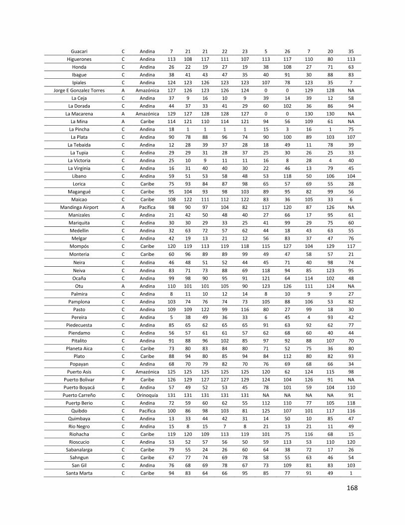
Guacari C Andina 7 21 21 22 23 5 26 7 20 35 Higuerones C Andina 113 108 117 111 107 113 117 110 80 113

Honda C Andina 26 22 19 27 19 38 108 27 71 63 Ibague C Andina 38 41 43 47 35 40 91 30 88 83 Ipiales C Andina 124 123 126 123 123 107 78 123 35 7

Jorge E Gonzalez Torres A Amazónica 127 126 123 126 124 0 0 129 128 NA La Ceja C Andina 37 9 16 10 9 39 14 39 12 58

La Dorada C Andina 44 37 33 41 29 60 102 36 86 94 La Macarena A Amazónica 129 127 128 128 127 0 0 130 130 NA

La Mina A Caribe 114 121 110 114 121 94 56 109 61 NA La Pincha C Andina 18 1 1 1 1 15 3 16 1 75 La Plata C Andina 90 78 88 96 74 90 100 89 103 107

La Tebaida C Andina 12 28 39 37 28 18 49 11 78 39 La Tupia C Andina 29 29 31 28 37 25 30 26 25 33

La Victoria C Andina 25 10 9 11 11 16 8 28 4 40 La Virginia C Andina 16 31 40 40 30 22 46 13 79 45

Líbano C Andina 59 51 53 58 48 53 118 50 106 104 Lorica C Caribe 75 93 84 87 98 65 57 69 55 28

Magangué C Caribe 95 104 93 98 103 89 95 82 99 56 Maicao C Caribe 108 122 111 112 122 83 36 105 33 6

Mandinga Airport A Pacífica 98 90 97 104 82 117 120 87 126 NA Manizales C Andina 21 42 50 48 40 27 66 17 95 61 Mariquita C Andina 30 30 29 33 25 41 99 29 75 60 Medellin C Andina 32 63 72 57 62 44 18 43 63 55 Melgar C Andina 42 19 13 21 12 56 83 37 47 76

Mompós C Caribe 120 119 113 119 118 115 127 104 129 117 Monteria C Caribe 60 96 89 89 99 49 47 58 57 21

Neira C Andina 46 48 51 52 44 45 71 40 98 74 Neiva C Andina 83 71 73 88 69 118 94 85 123 95 Ocaña C Andina 99 98 90 95 91 121 64 114 102 48

Otu A Andina 110 101 101 105 90 123 126 111 124 NA Palmira C Andina 8 11 10 12 14 8 10 9 9 27

Pamplona C Andina 103 74 76 74 73 105 88 106 53 82 Pasto C Andina 109 109 122 99 116 80 27 99 18 30

Pereira C Andina 5 38 49 36 33 6 45 4 93 42 Piedecuesta C Andina 85 65 62 65 65 91 63 92 62 77 Piendamo C Andina 56 57 61 61 57 62 68 60 40 44

Pitalito C Andina 91 88 96 102 85 97 92 88 107 70 Planeta Aica C Caribe 73 80 83 84 80 71 52 75 36 80

Plato C Caribe 88 94 80 85 94 84 112 80 82 93 Popayan C Andina 68 70 79 82 70 76 69 68 66 34

Puerto Asis C Amazónica 125 125 125 125 125 120 62 124 115 98 Puerto Bolivar P Caribe 126 129 127 127 129 124 104 126 91 NA Puerto Boyacá C Andina 57 49 52 53 45 78 101 59 104 110 Puerto Carreño C Orinoquía 131 131 131 131 131 NA NA NA NA 91

Puertp Berio C Andina 72 59 60 62 55 112 110 77 105 118 Quibdo C Pacífica 100 86 98 103 81 125 107 101 117 116

Quimbaya C Andina 13 33 44 42 31 14 50 10 85 47 Rio Negro C Andina 15 8 15 7 8 21 13 21 11 49 Riohacha C Caribe 119 120 109 113 119 101 75 116 68 15 Rioscucio C Andina 53 52 57 56 50 59 113 53 110 120

Sabanalarga C Caribe 79 55 24 26 60 64 38 72 17 26 Sahngun C Caribe 67 77 74 69 78 58 55 63 46 54 San Gil C Andina 76 68 69 78 67 73 109 81 83 103

Santa Marta C Caribe 94 83 64 66 95 85 77 91 49 1

168

Santa Rosa De Cabal C Andina 3 17 20 23 18 4 15 3 67 41 Santander De Quilichao C Andina 43 44 48 44 47 35 41 44 22 68

Santuario C Andina 27 14 27 15 16 33 25 32 24 52 Saravena C Orinoquía 117 113 112 117 112 106 90 115 119 29

Sevilla C Andina 65 54 54 59 51 77 73 64 92 119 Sincelejo C Caribe 52 84 78 75 87 51 67 51 70 22 Socorro C Andina 74 66 63 70 63 74 111 76 90 109

Sogamoso C Andina 69 58 58 64 56 69 29 70 94 105 Tame A Orinoquía 121 116 114 120 114 114 80 122 125 NA

Tierralta C Caribe 105 115 115 115 115 86 114 98 84 112 Tolúviejo C Caribe 55 72 67 63 76 42 37 52 51 24

Tuluá C Andina 19 40 47 43 39 17 76 20 38 31 Tumaco C Caribe 130 130 130 130 130 0 0 127 120 13

Tunja C Andina 62 47 41 51 43 72 65 67 69 114 Turbaco C Caribe 45 23 8 8 49 26 11 41 3 3 Turbo C Caribe 64 100 108 101 100 50 9 66 37 20 Ubaté C Andina 49 18 12 20 15 55 79 48 39 101 Uribia C Caribe 118 124 116 118 126 88 59 118 34 14

Valledupar C Caribe 101 110 105 107 108 119 48 102 116 32 Villa Garzon Airport A Andina 116 117 121 121 117 109 122 117 97 NA

Villavicencio C Andina 70 36 28 39 36 70 96 71 50 78 Yopal C Orinoquía 111 99 95 108 93 122 116 120 109 97

Zanjón Rico C Andina 28 34 37 35 42 23 35 25 29 53 Zarzal C Andina 22 39 46 45 34 29 70 19 43 79

Zipaquirá C Andina 24 6 5 6 5 31 42 18 21 88

Ecuador (n=47) Type Region Infra Loc Night Comp Decay Infra: 100 km

Loc: 100 km

Infra: 200 km

Loc: 200 km

Func

Alfaro C Costa 2 1 1 1 1 6 1 2 1 4 Ambato C Sierra 18 17 15 16 16 18 28 16 27 27

Atuntaqui C Sierra 1 13 12 12 10 1 20 1 9 12 Azogues C Sierra 23 20 17 19 20 24 4 25 21 26

Babahoyo C Costa 15 8 8 10 8 16 19 14 10 13 Boliche C Costa 11 4 7 8 5 15 15 10 7 7

Buena Fe C Costa 9 11 18 14 12 14 6 9 22 19 Cayambe C Sierra 13 14 11 13 13 7 21 13 11 30

Chone C Costa 32 30 31 31 30 32 29 30 35 32 Coca C Oriente 44 43 42 44 43 43 39 41 46 37

Colorado C Costa 29 23 27 26 24 29 7 32 19 6 Coronel E Carvajal A Oriente 37 38 37 38 38 39 42 37 42 NA

Cotopaxi International Airport A Sierra 17 7 6 7 7 10 16 18 6 NA Cuenca C Sierra 22 32 29 32 32 27 27 21 31 18 Daule C Costa 16 3 3 6 3 20 8 17 5 16

Esmeraldas C Costa 38 37 39 37 37 44 31 44 40 14 Gualaceo C Sierra 28 29 20 25 27 28 9 27 24 31

Gualaquiza A Oriente 41 40 40 41 40 36 44 39 43 NA Guaranda C Sierra 30 26 26 28 28 31 36 26 34 36 Guayaquil C Costa 4 9 10 3 9 8 3 4 8 5

Ibarra C Sierra 6 24 24 21 21 3 30 6 15 9 Jipijapa C Costa 25 12 13 18 14 25 11 29 12 20

Jose Maria Velasco Ibarra A Sierra 45 45 45 45 45 45 45 45 44 NA km 192 A Costa 33 33 34 33 33 38 23 34 32 NA

La Tacunga C Sierra 14 10 9 9 11 12 25 15 18 28 Loja C Sierra 40 41 41 42 41 37 43 40 41 24

169

Machala C Costa 20 34 33 34 34 17 17 23 29 1 Maragrosa A Costa 31 27 28 29 29 26 40 31 25 NA

Nono C Sierra 12 6 5 5 6 11 13 12 4 23 Nueva Loja C Oriente 43 44 44 43 44 41 33 43 45 35

Otavalo C Sierra 7 16 16 15 15 4 24 7 13 15 Pasaje C Costa 21 25 30 23 22 21 10 24 20 3

Portoviejo C Costa 24 19 25 22 18 23 5 28 17 10 Pte De Integración B Oriente 47 47 47 47 47 0 0 47 47 NA

Puyo C Oriente 34 35 35 35 35 33 34 33 36 39 Quevedo C Costa 10 15 23 20 17 13 32 11 28 17

Quito C Sierra 3 28 14 11 25 2 18 3 14 21 Riobamba C Sierra 26 22 19 24 26 30 26 20 33 29

Santa Elena C Costa 35 21 21 30 23 0 0 36 16 11 Santa Rosa C Costa 27 31 32 27 31 19 14 22 26 2

Santo Domingo De Los Colorados C Sierra 19 18 22 17 19 22 38 19 23 25 Tahuaico C Sierra 8 5 4 4 4 9 12 8 3 33 Tarapoa A Oriente 46 46 46 46 46 42 35 46 30 NA

Tena C Oriente 36 36 36 36 36 35 41 35 39 34 Tulcan C Sierra 39 39 38 39 39 34 37 38 37 8

Tumbaco C Sierra 5 2 2 2 2 5 2 5 2 22 Zamora C Oriente 42 42 43 40 42 40 22 42 38 38

Peru (n=78) Type Region Infra Loc Night Comp Decay Infra: 100 km

Loc: 100 km

Infra: 200 km

Loc: 200 km

Func

Abancay C Sierra 68 57 57 60 62 58 68 70 63 59 Alferez Vladimir Sara Bauer A Selva 76 76 76 76 76 NA NA NA NA NA

Andahuaylas C Sierra 66 50 53 59 59 67 59 69 71 45 Arequipa C Sierra 65 61 58 58 68 64 54 63 60 29 Atalaya A Selva 72 55 56 69 60 0 0 75 73 NA

Aucayacu C Selva 47 34 43 48 41 44 42 56 54 58 Ayacucho C Sierra 60 35 37 50 44 70 67 68 68 53

Bahia San Nicolas P Costa 54 31 31 39 33 47 25 64 17 NA Bambamarca C Sierra 51 52 54 57 56 56 56 48 67 47

Cajamarca C Sierra 49 47 51 55 55 49 58 42 66 34 Callao C Costa 9 5 5 3 5 9 20 10 6 12

Cerro De Pasco C Sierra 40 21 21 29 26 61 50 33 70 55 Chachapoyas C Sierra 64 71 71 71 71 66 71 59 74 38 Chaclacayo C Costa 10 1 1 2 1 10 8 9 2 26

Chiclayo C Costa 8 32 34 22 20 8 5 8 21 4 Chimbote C Costa 31 23 23 25 29 0 0 60 29 20

Chincha Alta C Costa 17 13 12 12 13 23 35 19 45 35 Chiu-Chiu C Costa 12 12 11 13 12 19 21 14 41 31

Chulucanas C Costa 22 37 36 35 35 18 36 16 27 19 Comandante Fap German Arias Graziani A Sierra 23 28 28 34 27 25 4 25 37 NA

Cuzco C Sierra 69 67 65 67 69 71 69 71 64 50 Francisco Carle A Sierra 21 16 14 14 14 24 18 20 53 NA

Guadalupe C Costa 14 26 26 19 23 15 29 18 14 27 Huacho C Costa 2 8 8 10 9 4 3 3 24 23

Huamachuco C Sierra 53 38 46 47 47 69 63 57 58 54 Huancabamba A Sierra 56 63 61 65 64 50 65 47 65 NA Huancavelica C Sierra 50 30 30 41 31 55 62 54 49 60

Huancayo C Sierra 28 17 20 18 18 30 19 27 57 49 Huanuco C Selva 37 25 29 36 30 61 50 50 55 39

Huaral C Costa 11 6 6 8 7 11 33 11 8 25

170

Huaraz C Sierra 20 24 24 30 25 22 10 23 40 41 Iberia A Selva 75 75 75 75 75 0 0 73 50 NA

Ica C Costa 35 20 18 23 22 43 43 52 39 42 Ilo C Costa 59 54 42 44 52 52 38 53 52 5

Imperial C Costa 18 9 9 11 11 37 24 17 32 36 Jaén C Selva 52 62 63 63 65 59 66 51 69 51

Juanjui A Selva 61 59 64 64 61 63 53 58 59 NA Juliaca C Sierra 44 49 48 32 45 39 15 38 42 22

Lambayeque C Costa 7 10 10 7 6 7 2 7 3 3 Lima C Costa 5 11 16 6 10 5 17 5 7 14 Lurín C Costa 3 3 3 4 3 1 12 1 4 17

Machu Pichu Airport A Sierra 73 70 66 68 70 68 70 72 72 NA Maria Reiche Neuman Airport A Costa 46 27 25 27 28 47 25 61 12 NA

Mayobamba C Selva 36 66 70 61 58 21 40 34 20 44 Mollendo C Costa 63 44 33 33 46 64 54 65 25 28

Moquegua C Sierra 58 53 44 42 53 52 38 49 56 15 Pacasmayo C Costa 16 29 27 21 24 16 44 24 16 32

Pachacamac C Costa 4 4 4 5 4 2 13 4 5 9 Paita C Costa 29 36 35 31 32 20 28 26 9 8

Peralvillo C Costa 1 7 7 9 8 3 1 2 18 24 Pisco C Costa 25 15 13 17 16 27 27 32 19 33 Piura C Costa 15 45 45 45 42 13 32 12 34 6

Pte De Integración B 67 73 72 74 73 57 64 62 75 NA Pucallpa C Selva 70 56 59 70 63 0 0 74 61 56

Puente Piedra C Costa 6 2 2 1 2 6 9 6 1 11 Puerto Bayovar P Costa 34 41 47 43 40 45 47 36 33 NA

Puerto Cabo Blanco P Costa 41 58 55 54 54 36 45 31 31 NA Puerto Esperanza A Selva 77 77 77 77 77 NA NA NA NA NA

Puerto Maldonado C Selva 74 74 74 72 74 51 60 67 48 57 Pues To Grau C Costa 48 65 67 53 50 32 6 35 26 1

Puno C Sierra 45 46 39 28 39 39 15 37 36 30 Punta Lobitos (Bahia De Huarmey) P Costa 27 18 17 20 19 46 57 45 30 NA

Rioja C Sierra 38 60 69 52 51 26 11 30 23 46 San Luis C Costa 13 22 22 16 17 12 14 13 11 10 Iquitos C Selva 78 78 78 78 78 NA NA NA NA 40

San Ramon A Selva 33 19 19 24 21 41 48 46 43 NA Santa Lucia Pnp Airstrip A Selva 39 39 50 49 43 31 22 41 35 NA

Sullana C Costa 26 43 41 40 38 17 34 21 13 21 Tacna C Costa 55 48 38 26 37 34 37 39 10 13 Talara C Costa 32 51 49 46 49 28 46 28 22 7

Tambo Grande C Costa 19 40 40 37 34 14 30 15 15 16 Tarapoto C Selva 57 64 68 66 66 38 52 55 28 43

Tarma C Sierra 24 14 15 15 15 29 31 22 51 48 Tocache Airport A Selva 42 42 52 51 48 35 23 40 44 NA

Trujillo C Costa 30 33 32 38 36 60 49 43 46 18 Tumbes C Costa 43 68 62 62 57 32 6 29 38 2 Yunguyo C Sierra 62 69 60 56 67 42 41 44 62 37

Yurimaguas C Selva 71 72 73 73 72 54 61 66 47 52

Source: Authors’ compilation

171

the world bank latin america and the …pubdocs.worldbank.org/en/780311492653985192/p... ·...

Documents