the xmm-newton serendipitous surveyxmmssc.irap.omp.eu/3xmm_v10.pdf · the xmm-newton serendipitous...
TRANSCRIPT
Astronomy & Astrophysics manuscript no. 3XMM_v10 c©ESO 2015April 27, 2015
The XMM-Newton serendipitous survey⋆
VII. The third XMM-Newton serendipitous source catalogue
S. R. Rosen1, N. A. Webb2, 3, M. G. Watson1, J. Ballet4, D. Barret2, 3, V. Braito1, 6, F. J. Carrera5, M. T. Ceballos5, M.Coriat2, 3, R. Della Ceca6, G. Denkinson1, P. Esquej1, S. A. Farrell1, M. Freyberg7, F. Grisé8, P. Guillout8, L. Heil1, D.Law-Green1, G. Lamer10, D. Lin2, 3, 12, R. Martino4, L. Michel8, C. Motch8, A. Nebot Gomez-Moran8, C. G. Page1, K.
Page1, M. Page11, M.W. Pakull8, J. Pye1, A. Read1, P. Rodriguez9, M. Sakano1, R. Saxton9, A. Schwope10, A. E.Scott1, R. Sturm7, I. Traulsen10, V. Yershov11, and I. Zolotukhin2, 3
1 Department of Physics & Astronomy, University of Leicester , Leicester, LE1 7RH, UK2 Université de Toulouse; UPS-OMP, IRAP, Toulouse, France
e-mail: [email protected] CNRS, IRAP, 9 av. Colonel Roche, BP 44346, F-31028 Toulouse cedex 4, France4 Laboratoire AIM, CEA-IRFU/CNRS/Université Paris Diderot, Service d’Astrophysique, CEA Saclay, 91191 Gif sur Yvette,
France5 Instituto de Fisica de Cantabria (CSIC-UC), Avenida de los Castros, 39005 Santander, Spain6 INAF-Osservatorio Astronomico di Brera, via Brera 28, I-20121 Milano, Italy7 Max-Planck-Institut für extraterrestrische Physik, Giessenbachstr., 85748 Garching, Germany8 Observatoire astronomique de Strasbourg, Université de Strasbourg, CNRS, UMR 7550, 11 rue de l’Université, F-67000 Stras-
bourg, France9 XMM SOC, ESAC, Apartado 78, 28691 Villanueva de la Cañada, Madrid, Spain
10 Leibniz-Institut for Astrophysics Potsdam (AIP), An der Sternwarte 16, 14482 Potsdam, Germany11 Mullard Space Science Laboratory, University College London, Holbury St Mary, Dorking, Surrey RH5 6NT, UK12 Institute for the Study of Earth, Oceans, and Space, University of New Hampshire, 8 College Road, Durham, NH 03824-2600,
U.S.A.
Received ; accepted
ABSTRACT
Context. Thanks to the large collecting area (3 × ∼1500 cm2 at 1.5 keV) and wide field of view (30′ across in full field mode) ofthe X-ray cameras on board the European Space Agency X-ray observatory XMM-Newton, each individual pointing can result in thedetection of up to several hundred X-ray sources, most of which are newly discovered objects. As XMM-Newton has now been inorbit for more than 15 years, hundreds of thousands of sources have been detected.Aims. Recently, many improvements in the XMM-Newton data reduction algorithms have been made. These include enhanced sourcecharacterisation and reduced spurious source detections, refined astrometric precision of sources, greater net sensitivity for source de-tection and the extraction of spectra and time series for fainter sources, with better signal-to-noise. Thanks to these enhancements, thequality of the catalogue products has been much improved with respect to earlier catalogues. Further, almost 50% more observationsare in the public domain compared to 2XMMi-DR3, allowing the XMM-Newton Survey Science Centre to produce a much larger andbetter quality X-ray source catalogue.Methods. The XMM-Newton Survey Science Centre has developed a pipeline to reduce the XMM-Newton data automatically. Usingthe latest version of this pipeline, along with better calibration, a new version of the catalogue has been produced, using XMM-NewtonX-ray observations made public on or before 2013 December 31. Manual screening of all of the X-ray detections ensures the highestdata quality. This catalogue is known as 3XMM.Results. In the latest release of the 3XMM catalogue, 3XMM-DR5, there are 565962 X-ray detections comprising 396910 uniqueX-ray sources. For the 133000 brightest sources, spectra and lightcurves are provided. For all detections, the positions on the sky, ameasure of the quality of the detection, and an evaluation of the X-ray variability is provided, along with the fluxes and count rates in7 X-ray energy bands, the total 0.2-12 keV band counts, and four hardness ratios. With an aim to identifying the detections, a crosscorrelation with 228 catalogues of sources detected in all wavebands is also provided for each X-ray detection.Conclusions. 3XMM-DR5 is the largest X-ray source catalogue ever produced. Thanks to the large array of data products associatedwith each detection and each source, it is an excellent resource in which to find new and extreme objects.
Key words. Catalogs – Astronomical data bases – Surveys – X-rays: general
⋆ Based on observations obtained with XMM-Newton, an ESA sci-ence mission with instruments and contributions directly funded byESA Member States and NASA.
1. Introduction
XMM-Newton (Jansen et al. 2001) is the second cornerstonemission from the European Space Agency Horizon 2000 pro-gramme. It was launched in December 1999 and thanks to the
Article number, page 1 of 20page.20

A&A proofs: manuscript no. 3XMM_v10
∼1500 cm2 of geometric effective area (Turner et al. 2001) foreach of the three X-ray telescopes aboard, it has the largest ef-fective area of any X-ray satellite (Longinotti 2014). This fact,coupled with the large field of view (FOV) of 30′, means that asingle pointing detects on average 50 to 100 serendipitous X-raysources (Watson et al. 2009).
For the last 19 years, the XMM-Newton Survey Science Cen-tre1 (SSC), a consortium of 10 European Institutes (Watson et al.2001) has developed much of the XMM-Newton Science Analy-sis Software (SAS)2 for reducing and analysing XMM-Newtondata and created pipelines to perform standardised routine pro-cessing of the XMM-Newton science data. The XMM SSC hasalso been responsible for producing catalogues of all of thesources detected with XMM-Newton. The catalogues of X-raysources detected with the three EPIC (Strüder et al. 2001a;Turner et al. 2001) cameras that are placed at the focal pointof the three X-ray telescopes, have been designated 1XMM and2XMM successively (Watson et al. 2009), with incremental ver-sions of these catalogues indicated by successive data releases,denoted -DR in association with the catalogue number. This pa-per presents the latest version of the XMM catalogue, 3XMM.The original 3XMM catalogue was data release 4 (DR4). Thepublication of this paper coincides with the release of 3XMM-DR5. This version includes one extra year of data and increasesthe number of detections by 7%, with respect to 3XMM-DR4.The number of X-ray detections in 3XMM-DR5 is 565962,which translate to 396910 unique X-ray sources. The medianflux of these X-ray sources is ∼2.4× 10⁻¹⁴ erg cm−2 s−1 (0.2-12.0keV) and the data taken span 13 years. The catalogue covers 877square degrees of sky (∼2.1% of the sky), if the overlaps in thecatalogue are taken into account. 3XMM-DR5 also includes anumber of enhancements with respect to the 3XMM-DR4 ver-sion which are described in appendix A. The 3XMM-DR5 cat-alogue is approximately 60% larger than the 2XMMi-DR3 re-lease and five times the current size of the Chandra source cata-logue (Evans et al. 2010). 3XMM uses significant improvementsto the SAS as well as incorporating developments with the cal-ibration. Enhancements include better source characterisation, alower number of spurious source detections, better astrometricprecision, greater net sensitivity and spectra and time series forfainter sources, with better signal-to-noise. These improvementsare detailed throughout this paper.
A separate catalogue of ultra-violet and optical sources de-tected with the XMM-Newton Optical Monitor (OM Mason et al.2001) is also produced in the framework of the XMM-NewtonSSC and is called the XMM-Newton Serendipitous Ultravio-let Source Survey (XMM-SUSS in its original form, with themore recent version named XMM-SUSS2, Page et al. 2012).XMM-SUSS2 contains 5 595 331 detections. They correspondto 4 008 879 sources, of which 692 223 have multiple pointings.This is a complementary catalogue to the 3XMM catalogue, asmany of the pointings are similar to those included in 3XMM,even if the FOV of the OM is smaller than the EPIC cameras.
3XMM is also complementary to other recent X-ray cata-logues such as the Chandra source catalogue mentioned above,and the 1SXPS (Swift-X-ray Telescope (XRT) point source) cat-alogue (Evans et al. 2014) of 151 524 X-ray point sources de-tected with the Swift-XRT over eight years of operation. 1SXPShas a sky coverage nearly 2.5 times that of 3XMM, but the ef-fective area of the XRT is less than a tenth of each of the tele-scopes on board XMM-Newton (Longinotti 2014). Other earlier
1 http://xmmssc.irap.omp.eu/2 http://xmm.esac.esa.int/sas/current/howtousesas.shtml
catalogues include all sky coverage, such as the ROSAT all-skysurvey (RASS Voges et al. 1999), but the reduced sensitivity ofROSAT compared to XMM-Newton means that the RASS cata-logue contains just 20% the number of sources in 3XMM-DR4.However, the different X-ray source catalogues in conjunctionwith 3XMM allow searches for long term variability. This is par-ticularly useful in the search for tidal disruption events (e.g. Linet al. 2011, 2013) and other transient objects such as the best can-didate for an intermediate mass black hole, ESO 243-49 HLX-1(Farrell et al. 2009; Webb et al. 2012). Nonetheless, a wide va-riety of other sources have also been found thanks to the XMMcatalogue, such as many new ultra luminous X-ray sources (Wal-ton et al. 2011), eclipsing polars (Vogel et al. 2008; Ramsay et al.2009), a peculiar isolated neutron star (Pires et al. 2012), distantluminous X-ray clusters (e.g. Lamer et al. 2008), etc.
Whilst this paper covers the 3XMM catalogues in gen-eral, some of the data validation presented was carried out onthe 3XMM-DR4 version that was made public on 23rd July2013. 3XMM-DR4 contains 531261 X-ray detections which re-late to 372728 unique X-ray sources, taken from 7427 XMM-Newton observations. The paper is structured as follows. Sec-tion 2 contains information concerning the observations used inthe 3XMM-DR5 catalogue. Section 3 covers the 3XMM dataprocessing and details changes made with respect to previouscatalogues (see Watson et al. 2009), such as the exposure selec-tion, the time-dependent boresight implemented, the suppressionof minimum ionizing particle (MIP) events, the optimised flarefiltering, the improved Point Spread Function (PSF) used for thesource detection, new astrometric corrections and the newly de-rived energy conversion factors (ECFs). We also outline the newsource flagging procedure. Section 4 covers the source specificproducts associated with the catalogue, such as the enhanced ex-traction methods for spectra and time series and the variabilitycharacterisation. Section 5 describes the various screening pro-cedures employed to guarantee the quality of the catalogue andSection 6 outlines the statistical methods used for identifyingunique sources in the database. Then, Section 7 describes theprocedures used to cross correlate all of the X-ray detectionswith external catalogues, Section 8 discusses the limitations ofthe catalogue and Section 9 characterises the enhancement ofthis catalogue with respect to previous versions, with the poten-tial of the catalogue highlighted by several examples of objectsthat can be found in 3XMM, in Section 10. Finally, informationon how to access the catalogue is given in Section 11, and futurecatalogue updates are outlined in Section 12, before concludingwith a Summary.
2. Catalogue observations
3XMM-DR5 is comprised of data drawn from 7781 XMM-Newton EPIC observations that were publicly available as of2013 December 31 and that processed normally. The Hammer-Aitoff equal area projection in Galactic coordinates of the3XMM-DR5 fields can be seen in Fig. 1. The data in 3XMM-DR5 include 440 observations that were publicly available at thetime of creating 2XMMi-DR3, but were not included in 2XMMi-DR3 due to the high background or processing problems. All ofthose observations containing > 1ks clean data (>1 ks of goodtime interval) were retained for the catalogue. Fig. 2 shows thedistribution of total good exposure time (after event filtering) forthe observations included in the 3XMM-DR5 catalogue, and us-ing any of the thick, medium or thin filters, but not the open filter.The number of the 7781 XMM-Newton observations included inthe 3XMM-DR5 catalogue for each observing mode and each
Article number, page 2 of 20page.20

S. R. Rosen et al.: The XMM-Newton serendipitous survey
Fig. 1. Hammer-Aitoff equal area projection in Galactic coordinates ofthe 7781 3XMM-DR5 fields.
Fig. 2. Distribution of total good exposure time (after event filtering)for the observations included in the 3XMM-DR5 catalogue (for eachobservation the maximum time of all three cameras per observation wasused).
filter is given in Table 1. Open filter data were processed but notused in the source detection stage of pipeline processing. Thesame XMM-Newton data modes were used as in 2XMM and areoutlined in Watson et al. (2009), their table 1.
The only significant difference was the inclusion of mo-saic mode data. Whilst most XMM-Newton observations are per-formed in pointing mode, where the spacecraft is locked on to afixed position on the sky for the entire observation, since revolu-tion 1812 (2009-Oct-30), a specific mosaic observing mode wasintroduced in which the satellite pointing direction is steppedacross the sky, taking snapshots at points (sub-pointings) on auser-specified grid. Data from dedicated mosaic mode or track-ing (mosaic-like) observations are recorded into a single Obser-vation Data File (ODF) for the observation. In previous pipelineprocessing, the pipeline products from the small number ofmosaic-like observations were generally generated, at best, for asingle sub-pointing only. This is because the pipeline filters datasuch that only events taken during an interval where the attitudeis stable and centred on the nominal observation pointing direc-tion (within a 3′ tolerance), are accepted. Data from some, orall, of the other sub-pointings were thus typically excluded. Dur-ing 2012, the XMM-Newton Science Operations Centre (SOC)devised a scheme whereby the parent ODF of a mosaic modeobservation is split into separate ODFs, one for each mosaicsub-pointing. All relevant data are contained within each sub-
pointing ODF and the nominal pointing direction is computedfor the sub-pointing. This approach is applied to both formalmosaic mode observations and those mosaic-like/tracking ob-servations executed before revolution 1812. For a mosaic modeobservation, the first 8 digits of its 10-digit observation identi-fier (OBS_ID) are common for the parent observation and itssub-pointings. However, while the last two digits of the par-ent observation OBS_ID almost always end in 01, for the sub-pointings they form a monotonic sequence, starting at 31. Mo-saic mode sub-pointings are thus immediately recognisable inhaving OBS_ID values whose last two digits are ≥ 31.
To the pipeline, mosaic mode (and mosaic-like) observationsub-pointings are transparent. No special processing is applied.Each sub-pointing is treated as a distinct observation. Source de-tection is performed on each sub-pointing separately and no at-tempt is made to simultaneously fit common sources detectedin overlapping regions of multiple sub-pointings. While simul-taneous fitting is possible, this aspect had not been sufficientlyexplored or tested during the preparations for the 3XMM cata-logues.
There are 45 observations performed in the dedicated mosaicmode before the bulk processing cut-off date of 2012-Dec-08, ofwhich 37 are included in 3XMM-DR5, see appendix A, point 1.None of these was available for catalogues prior to 3XMM. In to-tal, there are 356 processed mosaic sub-pointings in the 3XMM-DR5 catalogue.
3. Data processing
The data used for the 3XMM catalogues have been reprocessedwith the latest version of the SAS and the most up to date cali-bration available at the time of the processing. The majority ofthe processing for 3XMM-DR5 was conducted during December2012/January 2013, with the exception of 20 observations pro-cessed during 2013. The SAS used was similar to SAS 12.0.1but included some upgraded tasks required for the pipeline. TheSAS manifest for tasks used in the cat9.0 pipeline and the staticset of Current Calibration Files (CCFs) that were used for thebulk reprocessing are provided via a dedicated online webpage3.
There are 31 observations in 2XMMi-DR3 that did not makeit in to 3XMM-DR5, mainly due to software/pipeline errors dur-ing processing. Typical examples of the latter problems are dueto revised ODFs (e.g. with no useful time-correlation informa-tion), more sophisticated SAS software that identified issueshitherto not trapped, or issues with exposure corrections of back-ground flare light curves and pn time-jumps.
The main data processing steps used to produce the 3XMMdata products were similar to those outlined in Watson et al.(2009) and described on the SOC webpages4. In brief, thesesteps were the production of calibrated detector events from theODFs; identification of stable background time intervals; identi-fication of “useful” exposures (taking account of exposure time,instrument mode, etc.); generation of multi-energy-band X-rayimages and exposure maps from the calibrated events; sourcedetection and parameterisation; cross-correlation of the sourcelist with a variety of archival catalogues, image databases andother archival resources; creation of binned data products; appli-cation of automatic and visual screening procedures to check forany problems in the data products. The data from this process-
3 http://xmmssc-www.star.le.ac.uk/public/pipeline/doc/04_cat9.0_20121220.15384 http://xmm.esac.esa.int/sas/current/howtousesas.shtml
Article number, page 3 of 20page.20
A&A proofs: manuscript no. 3XMM_v10
Table 1. Characteristics of the 7781 XMM-Newton observations included in the 3XMM-DR5 catalogue.
Camera Modes Filters TotalFulla Windowb Otherc Thin Medium Thick
pn 5853 495 - 3327 2633 388 6348MOS1 6045 1306 309 3296 3774 590 7660MOS2 6100 1341 248 3303 3789 597 7689
a Prime Full Window Extended (PFWE) and Prime Full Window (PFW) modes; b pn Prime Large Window (PLW) mode and any ofthe various MOS Prime Partial Window (PPW) modes; c other MOS modes (Fast Uncompressed (FU), Refresh Frame Store (RFS)).
ing have been made available through the XMM-Newton ScienceArchive5 (XSA).
3.1. Exposure selection
The only change applied for identifying exposures to be pro-cessed by the pipeline compared to that adopted in pre-cat9.0processing (Watson et al. (2009) - see their section 4.1), was theexclusion of any exposure taken with the Open filter. This wasdone because use of the Open filter leads to increased contamina-tion from optical light (optical loading). Eight exposures (fromfive observations) taken with the Open filter were excluded fromthe data publicly available for the 3XMM-DR5 catalogue.
3.2. Event list processing
Much of the pipeline processing that converts raw ODF event filedata from the EPIC instruments into cleaned event lists has re-mained unchanged from the pre-cat9.0 pipeline and is describedin section 4.2 of Watson et al. (2009). However, we describe 3alterations to the approach used for 2XMM.
3.2.1. Time-dependent boresight
Analysis by both the XMM-Newton SSC and the SOC estab-lished the presence of a systematic, cyclic (≈362 day) time-dependent variation in the offset of each EPIC (and OM andRGS) instrument boresight from their nominal pointing posi-tions, for each observation. This seasonal dependence is super-posed on a long term trend, the semi-amplitude of the seasonaloscillation being ≈1.2′′ in the case of the EPIC instruments (Ta-lavera et al. 2012). These variations of the instrument boresightshave been characterised by simple functions in calibration (Ta-lavera et al. 2012; Talavera & Rodríguez-Pascual 2014). The ori-gin of the variation is uncertain but might arise from heatingeffects in the support structures of the instruments and/or space-craft star-trackers - no patterns have been identified in the avail-able housekeeping temperature sensor data though these may notsample the relevant parts of the structure.
During pipeline processing of XMM-Newton observationsfor the 3XMM catalogues, corrections for this time-dependentboresight movement are applied to individual event positions ineach instrument, via the SAS task attcalc, based on the observa-tion epochs of the events.
3.2.2. Suppression of Minimum Ionizing Particle events inEPIC-pn data
High energy particles can produce electron-hole pairs in the sil-icon substrate of the EPIC-pn detector. While onboard process-ing and standard pn event processing in the pipeline removes
5 http://xmm.esac.esa.int/xsa/
most of these so-called Minimum Ionizing Particle (MIP) events(Strüder et al. 2001b), residual effects can arise when MIPs ar-rive during the pre-exposure offset-map analysis and can giverise to features that appear as low-energy noise in the pn detec-tor. Typically, these features are spatially confined to a clump ofa few pixels and appear only in band 1. However, in pre-cat9.0pipeline processing, such features were sometimes detected assources during source detection and these were not always rec-ognized and flagged during the manual flagging process outlinedin section 7.4 of Watson et al. (2009). The SAS task, eprejectwas incorporated into the pipeline processing for 3XMM and inmost cases corrects for these MIP events during processing of pnevents.
3.2.3. Optimised flare filtering
In previous pipeline processing (pre-cat9.0 pipelines), the recog-nition of background flares and the creation of Good Time In-tervals (GTIs) between them was as described in section 4.3 ofWatson et al. (2009), where the background light curves werederived from high energy data and the count rate thresholds fordefining the GTIs were based on (different) constant values foreach instrument. In the processing for 3XMM, two key changeshave been made.
Firstly, rather than adopting fixed count rate thresholds ineach instrument, above which data are rejected, an optimisa-tion algorithm has been applied that maximises the signal-to-noise (S/N) for the detection of point sources. Secondly, the lightcurves of the background data used to establish the count ratethreshold for excluding background flares are extracted in an’in-band’ (0.5-7.5 keV) energy range. This was done so that theprocess described below resulted in maximum sensitivity to thedetection of objects in the energy range of scientific interest.
The overall process for creating the background flare GTIsfor each exposure within each observation involved the follow-ing steps:
1. For each exposure, a high energy light curve (from 7 to 15keV for pn, > 14 keV for MOS) is created, as previously, andinitial background flare GTIs are derived using the optimizedapproach employed in the SAS task, bkgoptrate (see below).
2. Following the identification of bad pixels, event cleaning andevent merging from the different CCDs, an in-band imageis then created, using the initial GTIs to excise backgroundflares.
3. The SAS task, eboxdetect then runs on the in-band image todetect sources with a likelihood > 15 - this is already veryconservative as only very bright (likelihood≫ 100), variablesources are able to introduce any significant source variabil-ity component into the total count rate of the detector (accu-mulated from most of the field).
4. An in-band light curve is subsequently generated, excludingevents from circular regions of radius 60′′ for sources with
Article number, page 4 of 20page.20

S. R. Rosen et al.: The XMM-Newton serendipitous survey
count rates ≤0.35 counts/s or 100′′ for sources with countrates >0.35counts/s, centred on the detected sources.
5. The SAS task, bkgoptrate, is then applied to the light curveto find the optimum background rate cut threshold and this issubsequently used to define the final background flare GTIs.
The optimisation algorithm adopted, broadly follows thatused for the processing of ROSAT Wide Field Camera data forthe ROSAT 2RE catalogue (Pye et al. 1995). The process seeksto determine the background count rate threshold at which theremaining data below the threshold yields a S/N ratio, S =
Cs√Cb
,for a (constant) source that is a maximum. Here Cs is the num-ber of source counts and Cb is the number of background counts.Since we are interested, here, in finding the background rate cutthat yields the maximum S/N and are not concerned about theabsolute value of that S/N, then for background light curves withbins of constant width, as created by the pipeline processing, Scan be expressed as
S =N√∑
ri
(1)
where N is the number of bins with background count ratesbelow the threshold, rT , and ri is the count rate in time bin i: thesummation is over the time bins with a count rate < rT . Timebins are of 10s width for pn and 26s for MOS. The process sortsthe time bins in order of decreasing count rate. Starting from thehighest count rate bin, bins are sequentially removed, computingequation 1 at each step. With the count rate of the bin removed ateach step representing a trial background count rate cut thresh-old, this process yields a curve of S/N vs. background count ratecut threshold. The background cut corresponding to the peak ofthe S/N curve is thus the optimum cut threshold.
In figure 3 we show four examples of in-band backgroundtime series in the top row, accompanied by the respective S/Nvs. background-cut-threshold plots in the bottom row. The firstpanel in each row represents a typical observation (MOS1) withsome significant background flaring activity. The optimum cutlevel of 1.83 cts/s leads to the creation of GTIs that exclude por-tions of the observation where the background exceeds the cutthreshold. The second panels are for a pn observation with a sta-ble, low background level. The optimum cut in the backgroundincludes all the data and thus generates a GTI spanning the en-tire observation. This is also true for the third panels which showa MOS1 case where the background is persistently high (abovethe level where the whole observation would have been rejectedin pre-cat9.0 pipeline processing). The fourth panels are for anexample of a variable background which gives rise to a dou-ble peaked S/N v background-rate-cut curve. Here, raising thethreshold from ∼18 cts/s to ∼28 cts/s simply involves a steeplyrising background rate early in the observation, causing a dip inthe S/N verses background-rate-cut curve. However, as the ratecut threshold is increased above 30 cts/s, although the count rateis higher, a lot more exposure time is available, so the S/N curverises again and the optimum cut includes almost all the data. Itshould be emphasized that the fixed cut thresholds used for MOSand pn in previous XMM processings can not be directly com-pared to the optimised ones used here because of the change inenergy band being used to construct the background light curve.It is, however, worth noting that the fixed cuts used previouslyoften result in very similar GTIs to those generated by the opti-misation process described above. This is because the previousfixed instrument thresholds were based on analyses that sought
Fig. 3. Flare background light curves (top row) and their correspond-ing S/N vs. background cut threshold plots (bottom row). The leftmostpanels are for a typical observation with notable background flaring.The second pair of vertically aligned panels shows an example wherethe background has a persistently low level, while the third pair of pan-els reflects an example where the background is persistently high. Therightmost panels show an example of a variable background which givesrise to a double-peaked S/N vs. background-rate-cut curve. The verti-cal red lines in the lower panels indicate the optimum background-cut-threshold (i.e. the peak of the curve) derived for the light curves in thetop panels. In the upper panels the applied optimum cut-rate is alsoshown in red as horizontal lines.
to find a representative level for the majority of XMM-Newtonobservations.
We discuss some of the gains of using this optimisation ap-proach in section 9.3 and some known issues in section 8.
3.3. Source detection using the empirical Point SpreadFunction (PSF) fitting
The bulk reprocessing for 3XMM took advantage of new devel-opments related to the EPIC PSFs. The source detection stage inprevious pipelines (Watson et al. (2009) - see their section 4.4.3)made use of the so-called ’default’ (or medium accuracy) PSFfunctions determined by ray tracing of the XMM-Newton mir-ror systems. However, these default PSF functions recognizedno azimuthal dependence in the core of the source profile, didnot adequately describe the prominent spoke structures seen insource images (arising from the mirror support structures) andwere created identically for each EPIC camera.
To address the limitations of the default EPIC PSFs, a set ofempirical PSFs were constructed, separately for each instrument,by careful stacking of observed XMM source images over a gridof energy and off-axis angles from the instrument boresights.The cores and spoke patterns of the PSFs were then modelledindependently so that implementation within the XMM-NewtonSAS calibration software then enables PSFs to be reconstructedthat take into account the off-axis and azimuthal locations of asource, as well as the energy band. The details of the issues asso-ciated with the default PSF and the construction and validationof the empirical PSF are presented in Read et al. (2011).
The use of the empirical PSF has several ramifications insource detection. Firstly, the better representation of structuresin the real PSF results in more accurate source parameterisa-tion. Secondly, it helps reduce the number of spurious detec-
Article number, page 5 of 20page.20

A&A proofs: manuscript no. 3XMM_v10
tions found in the wings of bright sources. This is because theprevious medium accuracy PSFs did not adequately model thecore and spoke features, leaving residuals during fitting that wereprone to being detected as spurious sources. With the empiricalPSFs, fewer such spurious detections are found, especially in thewings of bright objects positioned at larger (> 6′) off-axis angles.Thirdly, as a result of the work on the PSFs, the astrometric ac-curacy of XMM-Newton source positions has been significantlyimproved (see Read et al. 2011).
3.3.1. Other corrections related to the PSF
During the late stages of testing of the pipeline used for the bulkreprocessing that fed into the 3XMM-DR4 catalogue, an analy-sis of XMM-Newton X-ray source positions relative to the high-accuracy (≤ 0.1′′) reference positions of SDSS (DR9) quasarsidentified a small but significant, off-axis-angle-dependent posi-tion shift, predominantly along the radial vector from the instru-ment boresight to the source. The effect, where the real sourceposition is closer to the instrument boresight than that inferredfrom the fitted PSF centroid, has a negligible displacement onaxis and grows to ∼0.65′′ at off-axis angles of 15′. This ra-dial shift is due to the displacement between the true positionof a source and the defined centroid (as determined by a 3-dimensional, circular, Gaussian fit to the model PSF profile) ofthe empirical PSF, which grows as the PSF becomes increasinglydistorted at high off-axis angles. It should be noted that identi-fying and measuring this effect has only been possible becauseof the corrections for other effects (see section 3.3 and below)that masked it, and because of the large number of sources avail-able that provide sufficient statistics. In due course a correctionfor this effect will be applied directly to event positions, on aper-instrument basis, via the XMM-Newton calibration system,but for the 3XMM-DR4 catalogue, to avoid delays in its produc-tion, a solution was implemented within the catcorr SAS task.A correction, computed via a third-order polynomial function, isapplied to the initial PSF-fitted coordinates of each source out-put by emldetect, i.e. prior to the field rectification step, basedon the off-axis angle of the source as measured from the space-craft boresight. This correction is embedded in the RA and DECcolumns, which also include any rectification corrections (sec-tion 3.4). The correction is computed and applied in the sameway for both the 3XMM-DR4 and 3XMM-DR5 catalogues.
A second PSF-related problem that affected 2XMMi-DR3positions was uncovered during early testing of the empiricalPSF (see Read et al. 2011). This arose from a 0.5 pixel error(in both the x and y directions) in the definition of the pixel co-ordinate system of the medium-accuracy PSF map - as pixels inthe PSF map are defined to be 1′′ x 1′′, the error is equivalentto 0.5′′ in each direction. When transferred to the image frameduring PSF fitting in emldetect, this error in the PSF map coor-dinate system manifested itself as an offset of up to 0.7′′ in theRA/DEC of a source position, varying with azimuthal positionwithin the field. The introduction of the empirical PSF removesthis error.
3.4. Astrometric rectification
3.4.1. Frame correction
Celestial coordinates of sources emerging from the PSF fittingstep of pipeline processing of a given observation include a gen-erally small systematic error arising from offsets in the space-craft boresight position from the nominal pointing direction for
the observation. The uncertainty is due to imprecisions in theattitude solution derived from data from the spacecraft’s star-trackers and may result in frame shifts that are typically ∼1′′ (butcan be as much as 10′′ in a few cases) in the RA and DEC direc-tions and a rotation of the field about the boresight of the orderof 0.1 degrees. To correct for (i.e. rectify) these shifts, an attemptis made to cross-correlate sources in the XMM-Newton field ofview with objects from an astrometric reference catalogue. X-raysources with counterparts in the reference catalogue are used toderive the frame shifts and rotation that minimise the displace-ments between them. In all previous pipeline processing (andcatalogues derived from them) these frame corrections were es-timated using the SAS task, eposcorr, which used a single refer-ence catalogue, USNO-B1.0, and the SAS task, evalcorr, to de-termine the success and reliability of the outcome (Watson et al.(2009) - see their section 4.5).
The processing system used to create the data for the3XMM catalogues makes use of some important improvementsto this field rectification procedure, which are embedded in thenew SAS tasks, catcorr that replaces eposcorr and evalcorr.Firstly, the new approach incorporates an iterative fitting func-tion (Nelder & Mead 1965) to find the optimum frame-shift cor-rections: previously the optimum shift was obtained from a grid-search procedure. Secondly, the cross-match between XMM-Newton and reference catalogue source positions is carried outusing three reference catalogues: (1) USNO-B1.0 (Monet et al.2003), (2) 2MASS (Skrutskie et al. 2006) and, where sky cov-erage permits, (3) the Sloan Digital Sky Survey (DR9) (Abaza-jian et al. 2009). The analysis is conducted using each catalogueseparately. When there is an acceptable fit from at least one cat-alogue, the RA and DEC frame shifts and the rotation derivedfrom the ’best’ case are used to correct the source positions. A fitis considered acceptable if there are at least 10 X-ray/counterpartpairs, the maximum offset between a pair (X-ray source, i andcounterpart, j) is < 10′′ and the goodness of fit statistic
L =
nx∑
i=1
no∑
j=1
max(0.0, pi j − qi j) ≥ 5 (2)
where pi j = e−12 (ri j/σi j)2
and qi j = no(ri j/r f )2. Here, pi j is theprobability of finding the counterpart at a distance > ri j from theX-ray source position given the combined (in quadrature) posi-tional uncertainty, σi j, while qi j is the probability that the coun-terpart is a random field object within ri j. An estimate of the lo-cal surface density of field objects from the reference catalogueis made by counting the number, no, of such objects within a cir-cular region of radius r f (set to 1′) around each XMM source. nx
is the number of X-ray sources in the XMM field. The L statistic,which represents a heuristic approach to the problem of identi-fying likely matching counterparts, is computed over ths set ofmatching pairs and is a measure of the dominance of the close-ness of the counterparts over the probability of random matches.The shifts in RA and DEC and the rotation are adjusted withinthe fitting process to maximise L. Extensive trials found that ifL ≥ 5, the result is generally reliable. Where more than one ref-erence catalogue gives an acceptable solution, the one with thelargest L value is adopted.
In the 3XMM catalogues, the corrected coordinates areplaced in the RA and DEC columns; the original uncorrectedcoordinates are reported via the RA_UNC and DEC_UNCcolumns. A catalogue identifier for the catalogue yielding the’best’ result is provided in the REFCAT column. If the best fithas parameter values (e.g. the number of matches used) that fall
Article number, page 6 of 20page.20

S. R. Rosen et al.: The XMM-Newton serendipitous survey
below the specific constraints mentioned above, the original, un-corrected positions are retained (written to both the RA and DECand RA_UNC and DEC_UNC columns) and the REFCAT iden-tifier takes a negative value. Further details may be found inthe documentation for the catcorr task. This new rectificationalgorithm is successful for about 83% of observations, whichcontain 89% of detections, reflecting a significant improvementcompared to the previous approach where ∼ 65% of fields couldbe corrected. The main gain comes from the use of the 2MASScatalogue which is particularly beneficial in obtaining rectifica-tion solutions in the galactic plane - it should be pointed out thatsimilar gains would be obtained with eposcorr if used with theexpanded set of reference catalogues. It should be noted that theextracted lists of objects from each of the three reference cat-alogues that lie within the full EPIC field of view for a givenobservation, are provided to users of XMM-Newton data prod-ucts via the file-type=REFCAT product file, which is used bythe task, catcorr.
3.4.2. Systematic position errors
As discussed in section 9.5 of Watson et al. (2009), for the2XMM catalogue (and relevant to subsequent incremental cat-alogues in the 2XMM series), the angular deviations of SDSS(DR5) quasars (Schneider et al. 2007) from their XMM-NewtonX-ray counterparts, normalised by the combined position er-rors, could not be modelled by the expected Rayleigh distribu-tion unless an additional systematic uncertainty (SYSERR pa-rameter in 2XMM) was added to the statistical position error(RADEC_ERR parameter in 2XMM) derived during the PSF fit-ting process. Watson et al. (2009) showed that this systematicwas not consistent with the uncertainty arising from the rectifi-cation procedure used for the 2XMM processing and ultimatelyadopted an empirically-determined systematic error value thatproduced the best match between the distribution of XMM-quasar offsets and the expected Rayleigh curve.
As part of the upgrade applied to the rectification processfor the bulk reprocessing used for the 3XMM catalogues, theuncertainty arising from this step has been computed, in partic-ular, taking into account the error component arising from therotational offset. Errors (1σ) in each component, i.e., on the RAoffset, ∆αc, on the DEC offset (∆δc) and on the rotational an-gle offset (∆φc), have been combined in quadrature to give anestimate of the total positional uncertainty, ∆r, arising from therectification process as
∆r = [(∆αc)2 + (∆δc)2 + (θc.∆φc)2]
12 (3)
where θc is the radial off-axis angle, measured in the sameunits as ∆αc and ∆δc and ∆φc is in radians.
Inclusion of this rectification error (column SYSERRCC inthe 3XMM catalogues), in quadrature with the statistical er-ror, leads to a generally good agreement between the XMM-quasar offset distribution and the expected Rayleigh distribu-tion compared to the previous approach and indicates that theempirically-derived systematic used in pre-3XMM catalogues isno longer needed. This is discussed further in section 9.2.
3.5. Energy Conversion Factors (ECFs)
A number of improvements in the calibration of the MOS and pninstruments have occurred since the previous, 2XMMi-DR3, cat-alogue was produced, which lead to slight changes in the Energy
Conversion Factors (ECFs) that are used for converting countrates in the EPIC energy bands to fluxes (see Watson et al. (2009)section 4.6). Of note is the fact that MOS redistribution matri-ces were provided for 13 epochs at the time of processing for3XMM and for three areas of the detector that reflect the so-called ’patch’, ’wings-of-patch’ and ’off-patch’ locations (Sem-bay et al. 2011).
For the 3XMM catalogues a simple approach has beenadopted. ECFs were computed following the prescription of Ma-teos et al. (2009), for energy bands 1 to 5 (0.2-0.5 keV, 0.5-1.0 keV, 1.0-2.0 keV, 2.0-4.5 keV and 4.5-12.0 keV respec-tively) and band 9 (0.5-4.5 keV), for full-frame mode, for eachEPIC camera, for each of the Thin, Medium and Thick filters.A power-law spectral model with a photon index, Γ = 1.7 anda cold absorbing column density of NH = 3 × 1020 cm−2 wasassumed. As such, users are reminded that the ECFs, and hencethe fluxes provided in the 3XMM catalogues, may not accuratelyreflect those for specific sources whose spectra differ apprecia-bly from this power-law model - see section 4.6 of Watson et al.(2009).
For pn, the ECFs are calculated at the on-axis position. Thepn response is sufficiently stable that no temporal resolution isneeded. For MOS, to retain a direct connection between theECFs and publicly available response files, the ECFs used aretaken at epoch 13 and are for the ’off-patch’ location. The lat-ter choice was made because the large majority of detectionsin an XMM-Newton field lie outside the ’patch’ and ’wings-of-patch’ regions, which only relate to a region of radius ≤ 40′′,near the centre of the field. The use of a single epoch (epoch 13)was made to retain simplicity in the processing and because theresponse of the MOS cameras exhibits a step function change(due to a gain change) between epochs 5 and 6, with differentbut broadly constant values either side of the step. None of the13 calibration epochs represent the average response and thusno response file exists to which average ECFs can be directly re-lated. The step-function change in the responses for MOS is mostmarked in band 1 (0.2-0.5 keV) for the ’patch’ location, wherethe maximum range in ECFs either side of the step amounts to20%. Outside the ’patch’ region, and for all other energy bands,the range of the ECF values with epoch is ≤ 5% and is ≤ 2.5%for the ’off-patch’ region. Epoch 13 was chosen, somewhat ar-bitrarily, as being typical of epochs in the longer post-step timeinterval.
The ECFs, in units of 1011 cts cm2 erg−1, adopted for the bulkreprocessing of data used for 3XMM, are provided in Table 2, foreach camera, energy band and filter. The camera rate, ca_RATE,and flux, ca_FLUX, are related via ca_FLUX = (ca_RATE/ECF)(where ca is PN, M1 or M2)
3.6. Updated flagging procedures
A significant issue in terms of spurious detections in XMM-Newton data arises from detections associated with Out-of-Time(OoT) events. For sources that do not suffer significantly frompile-up, the background map used by emldetect includes a com-ponent that models the OoT features. However, for sourceswhere pile up is significant, the OoT modelling is inadequate.This can give rise to spurious sources being detected along OoTfeatures. For the more piled up objects, the numbers of spuriousdetections along OoT features can become large (tens to hun-dreds).
Another feature arising from bright sources that affects theMOS instruments is scattered X-rays from the Reflection Grat-ing Arrays (RGA). These manifest themselves as linear features
Article number, page 7 of 20page.20

A&A proofs: manuscript no. 3XMM_v10
Table 2. Energy conversion factors (in units of 1011 cts cm2 erg−1) usedto convert count rates to fluxes for each instrument, filter and energyband
FiltersCamera Band Thin Medium Thickpn 1 9.52 8.37 5.11
2 8.12 7.87 6.053 5.87 5.77 4.994 1.95 1.93 1.835 0.58 0.58 0.579 4.56 4.46 3.76
MOS1 1 1.73 1.53 1.002 1.75 1.70 1.383 2.04 2.01 1.794 0.74 0.73 0.705 0.15 0.15 0.149 1.38 1.36 1.20
MOS2 1 1.73 1.52 0.992 1.76 1.71 1.393 2.04 2.01 1.794 0.74 0.73 0.705 0.15 0.15 0.159 1.39 1.36 1.21
in MOS images passing through the bright object, rather similarin appearance to OoT features. These features are not modelledat all in the background map.
In previous catalogues, spurious detections associated withOoT and RGA features have simply been masked during manualscreening. In the cat9.0 pipeline, for the first time, an attempt hasbeen made to identify the presence of OoT and RGA featuresfrom piled up sources and to flag detections that are associatedwith them.
The SAS task, eootepileupmask, is used for this purpose.This task uses simple instrument (and mode) -dependent pre-defined thresholds to test pixels in an image for pile-up. Whereit detects pixels that exceed the threshold, the column containingthat pixel is flagged in a mask map for the instrument. The taskattempts to identify and mask columns and rows associated withsuch pixels in OoT and RGA features.
Once the pile up masks are generated, the SAS task, dpssflagis used to set flag 10 of the PN_FLAG, M1_FLAG, M2_FLAG,EP_FLAG columns in the catalogues for any detection whosecentre lies on any masked column or row.
4. Source-specific product generation
4.1. Optimised spectral and time series extraction
The pipeline processing automatically extracts spectra and timeseries (source-specific products, SSPs), from suitable exposures,for detections that meet certain brightness criteria.
In pre-cat9.0 pipelines, extractions were attempted for anysource which had at least 500 EPIC counts. In such cases, sourcedata were extracted from a circular aperture of fixed radius (28′′),centred on the detection position, while background data wereaccumulated from a co-centred annular region with inner andouter radii of 60′′ and 180′′, respectively. Other sources that laywithin or overlapped the background region were masked duringthe processing. In most cases this process worked well. However,in some cases, especially when extracting SSPs from sourceswithin the small central window of MOS Small-Window modeobservations, the background region could comprise very littleusable background, with the bulk of the region lying in the gap
between the central CCD and the peripheral ones. This resultedin very small (or even zero) areas for background rate scalingduring background subtraction, often leading to incorrect back-ground subtraction during the analysis of spectra in XSPEC (Ar-naud 1996).
For the bulk reprocessing leading to the 3XMM catalogues,two new approaches have been adopted and implemented in thecat9.0 pipeline.
1. The extraction of data for the source takes place from anaperture whose radius is automatically adjusted to maximisethe signal-to-noise (S/N) of the source data. This is achievedby a curve-of-growth analysis, performed by the SAS task,eregionanalyse. This is especially useful for fainter sourceswhere the relative important of the background level ishigher.
2. To address the problem of locating an adequately filled back-ground region for each source, the centre of a circular back-ground aperture of radius, rb = 168′′ (comparable area tothe previously used annulus) is stepped around the sourcealong a circle centred on the source position. Up to 40 uni-formly spaced azimuthal trials are tested along each circle.A suitable background region is found if, after masking outother contaminating sources that overlap the background cir-cle and allowing for empty regions, a filling factor of atleast 70% usable area remains. If none of the backgroundregion trials along a given circle yields sufficient residualbackground area, the background region is moved out to acircle of larger radius from the object and the azimuthal tri-als are repeated. The smallest trial circle has a radius, rc, ofrc = rb +60′′ so that the inner edge of the background regionis at least 60′′ from the source centre - for the case of MOSSmall-Window mode, the smallest test circle for a source inthe central CCD is set to a radius that already lies on theperipheral CCDs. Other than for the MOS Small-Windowcases, a further constraint is that, ideally, the background re-gion should lie on the same instrument CCD as the source.If no solution is found with at least a 70% filling factor, thebackground trial with the largest filling factor is adopted.For the vast majority of detections where SSP extraction isattempted, this process obtains a solution in the first radialstep and a strong bias to early azimuthal steps, i.e. in mostcases an acceptable solution is found very rapidly. For detec-tions in the MOS instruments, about 1.7% lie in the centralwindow in Small-Window mode and have a background re-gion located on the peripheral CCDs. Importantly, in contrastto earlier pipelines, this process always yields a usable back-ground spectrum for objects in the central window of MOSSmall-Window mode observations.This approach to locating the background region wasadopted primarily to provide a single algorithm that worksfor all sources, including those located in the MOS smallwindow, when used. However, a drawback relative to theuse of the original annular background region arises wheresources are positioned on a notably ramped or other spatiallyvariable background (e.g. in the wings of cluster emission),where the background that is subtracted can vary, dependingon which side of the source the background region is located.
In addition, the cat9.0 pipeline permits extraction of SSPs forfainter sources. Extraction is considered for any detection withat least 100 EPIC source counts (EP_8_CTS). Where this condi-tion is met, a spectrum from the source aperture (i.e. source plusbackground) is extracted. If the number of counts from spectrum
Article number, page 8 of 20page.20
S. R. Rosen et al.: The XMM-Newton serendipitous survey
channels not flagged as ’bad’ (in the sense adopted by XSPEC) is> 100, a spectrum and time series are extracted for the exposure.The initial filter on EPIC counts is used to limit the processingtime as, for dense fields, the above background location processcan be slow.
4.2. Attitude GTI filtering
Occasionally, the spacecraft can be settling on to, or begin mov-ing away from, the intended pointing direction within the nom-inal observing window of a pointed XMM-Newton observation,resulting in notable attitude drift at the start or end of an expo-sure. Image data are extracted from events only within ’GoodTime Intervals’ (GTIs) when the pointing direction is within 3′
of the nominal pointing position for the observation. However, inpre-cat9.0 pipelines, spectra and time series have been extractedwithout applying such attitude GTI filtering. Occasionally, thisresulted in a source location being outside or at the edge of thefield of view when some events were being collected, leadingto incorrect transitions in the time series. In some cases, thesetransitions gave rise to the erroneous detection of variability insubsequent time series processing. In the cat9.0 pipeline, attitudeGTI filtering is applied during the extraction of spectra and timeseries.
4.3. Variability characterisation
As with pre-cat9.0 pipeline processing, the pipeline processingfor the 3XMM catalogues subjects each extracted exposure-levelsource time series to a test for variability. This test is a simpleχ2 analysis for the null hypothesis of a constant source countrate (Watson et al. (2009) - see their section 5.2). Sources with aprobability ≤ 10−5 of being constant have been flagged as beingvariable in previous XMM-Newton X-ray source catalogues andthis same approach is adopted for 3XMM.
In addition, for 3XMM, we have attempted to characterisethe scale of the variability through the fractional variabilityamplitude, Fvar (provided via the PN_FVAR, M1_FVAR andM2_FVAR columns and associated FVARRERR columns), whichis simply the square root of the excess variance, after normalisa-tion by the mean count rate, 〈R〉, i.e.
Fvar =
√
(S 2 − 〈σerr2〉)
〈R〉2(4)
(e.g. Edelson et al. (2002); Nandra et al. (1997) and refer-ences therein), where S 2 is the observed variance of the timeseries with N bins, i.e.
S 2 =1
N − 1
N∑
i=1
(Ri − 〈R〉)2
in which Ri is the count rate in time bin i. For the calcula-tion of the excess variance, (S 2 − 〈σerr
2〉), which measures thelevel of observed variance above that expected from pure datameasurement noise, the noise component, 〈σerr
2〉, is computedas the mean of the squares of the individual statistical errors, σ2
i,
on the count rates of each bin, i, in the time series.The uncertainty, ∆(Fvar), on Fvar, is calculated following
equation B2 in appendix B of Vaughan et al. (2003), i.e.
∆(Fvar) =
[(
√
12N
〈σerr2〉
〈R〉2Fvar
)2
+
(
√
〈σerr2〉
N
1〈R〉
)2] 12
This takes account of the statistical errors on the time binsbut not scatter intrinsic to the underlying variability process.
5. Screening
As for previous XMM-Newton X-ray source catalogues (Watsonet al. (2009) - see section 7), every XMM-Newton observationin the 3XMM catalogues has been visually inspected with thepurpose of identifying problematic areas where source detectionor source characterisation are potentially suspect. The manualscreening process generates mask files that define the problem-atic regions. These may be confined regions around individualsuspect detections or larger areas enclosing multiple affected de-tections, up to the full area of the field where serious problemsexist. Detections in such regions are subsequently assigned amanual flag (flag 11) in the flag columns (PN_FLAG, M1_FLAG,M2_FLAG, EP_FLAG). It should be noted that a detection withflag 11 set to (T)rue does not necessarily indicate that the detec-tion is considered to be spurious.
One significant change to the screening approach adopted for3XMM relates to the flagging of bright sources and detectionswithin a halo of suspect detections around the bright source. Pre-viously, all detections in the halo region, including the primarydetection of the bright source itself (where discernible), had flag11 set to True (manual flag) but the primary detection of thebright object itself, also had flag 12 set. The meaning of flag12 there was to signify that the bright object detection was notconsidered suspect. The use of flag 12 in this ’negative’ context,compared to the other flags, was considered to be potentiallyconfusing. For this reason, for the 3XMM catalogues, we havedropped the use of flag 12 and simply ensured that, where thebright object detection is clearly identified, it is un-flagged (i.e.neither flag 11 or 12 are set). Effectively, flag 12 is not used in3XMM. It should be noted that bright sources that suffer signifi-cant pile-up are not flagged in any way in 3XMM (or in previousXMM-Newton X-ray source catalogues).
The masked area of each image is an indicator of the qualityof the field as a whole. Large masked areas are typically associ-ated with diffuse extended emission, very bright sources whosewings extend across much of the image, or problems such as arcsarising from single-reflected X-rays from bright sources just out-side the field of view. The fraction of the field of view that ismasked is characterised by the observation class (OBS_CLASS)parameter. The distribution of the six observation classes in the3XMM catalogues has changed with respect to 2XMMi-DR3(see table 3). The dominant change is in the split of fields as-signed observation classes 0 and 1, with more fields that weredeemed completely clean in 2XMMi-DR3 having very small ar-eas (generally single detections) being marked as suspect in the3XMM catalogues. Often these are features that were consid-ered, potentially, to be unrecognised bright pixels, e.g. detec-tions dominated by a single bright pixel in one instrument withno similar feature in the other instruments. It should be empha-sised, however, that the manual screening process is unavoidablysubjective.
6. Catalogue construction: unique sources
The 3XMM detection catalogues collate all individual detectionsfrom the accepted observations. Nevertheless, since some fields
Article number, page 9 of 20page.20

A&A proofs: manuscript no. 3XMM_v10
Table 3. 3XMM observation classification (OBS_CLASS) (first col-umn), percentage of the field considered problematic (second column)and the percentage of fields that fall within each class for 2XMMi-DR3and 3XMM-DR5 (third and fourth columns respectively)
OBS CLASS masked fraction 2XMMi-DR3 3XMM-DR50 bad area = 0% 38% 27%1 0% < bad area < 0.1% 12% 22%2 0.1% < bad area < 1% 10% 12%3 1% < bad area < 10% 25% 24%4 10% < bad area < 100% 10% 11%5 bad area = 100% 5% 4%
have at least partial overlaps with others and some targets havebeen observed repeatedly with the target near the centre of thefield of view, many X-ray sources on the sky were detected morethan once (up to 48 times in the most extreme case). Individ-ual detections have been assigned to unique sources on the sky(i.e. a common unique source identifier, SRCID, has been al-located to detections that are considered to be associated withthe same unique source) using the procedure outlined here. Theprocess used in constructing the 3XMM catalogues has changedfrom that used for the 2XMM series of catalogues (Watson et al.(2009) - see their section 8.1).
The matching process is divided into two stages. The firststage finds, for each detection, all other matching detectionswithin 15′′ of it, from other fields (i.e. excluding detections fromwithin the same observation, which, by definition, are regardedas arising from distinct sources) and computes a Bayesian matchprobability for each pair as Budavári & Szalay (2008)
pmatch =
[
1 +1 − p0
B · p0
]−1
(5)
Here, B, the Bayes factor, is given by
B =2
(σ21 + σ
22)
exp−[
ψ2
2(σ21 + σ
22)
]
(6)
where σ1 and σ2 are the positional error radii of each detec-tion in the pair (in radians) and ψ is the angular separation be-tween them, in radians. p0 = N∗/N1N2 where N1 and N2 are thenumbers of objects in the sky based on the surface densities inthe two fields and N∗ is the number of objects common betweenthem. Each of these N values is derived from the numbers of de-tections in the two fields and are then scaled to the whole sky.The value of N∗ is not known, a priori, and in general can be ob-tained iteratively by running the matching algorithm. However,here we are matching observations of the same field taken withthe same telescope at two different epochs so that in most cases,objects will be common. Of course this assumption is affected bythe fact that the two observations being considered may involvedifferent exposure times, different instruments, filters and modesused and different boresight positions (with sources within theirfields of view being subject to different vignetting factors). Togauge the impact of such effects in determining N∗, trials us-ing an iterative scheme were run, which indicated that takingN∗ = 0.9min(N1,N2) provides a good estimate of N∗ without theneed for iteration. Finally, with all pairs identified and probabil-ities assigned, pairs with pmatch < 0.5 were discarded.
In the second, clustering stage, a figure-of-merit is computedfor each detection, referred to here as the goodness-of-clustering(GoC), which is the number of matches the detection has with
other detections, normalised by the area of its error circle radius(given by POSERR). This GoC measure prioritises detectionsthat lie towards the centre of a group of detections, and are thuslikely to be most reliably associated with a given unique source.The list of all detections is then sorted by this GoC value. Thealgorithm works down the GoC-sorted list and for each detec-tion, the other detections it forms pairs with are sorted by pmatch.Then, descending this list of pairs, for each one there are fourpossibilities for assigning the unique source identifiers: i) if bothdetections have previously been allocated to a unique source andalready have the same SRCID, nothing is done, ii) if neither havea SRCID, both are allocated the same, new SRCID, iii) if onlyone of them has already been assigned a SRCID, the other is al-located the same SRCID, iv) where both detections in the pairhave allocated but different SRCIDs, this represents an ambigu-ous case - for these, the existing SRCIDs are left unchanged buta confusion flag is set for both detections.
This approach is reliable in matching detections into uniquesources in the large majority of cases. Nevertheless, there aresituations where the process can fail or yield ambiguous results.Examples typically arise in complex regions, such as where spu-rious sources, associated with diffuse X-ray emission or brightsources, are detected and, by chance, are spatially close to thepositions of other detections (real or spurious) in other observa-tions of the same sky region. Often, in such cases, the detectionsinvolved will have manual quality flags set (Watson et al. (2009)- see their section 7.5 and also section 5 above).
Other scenarios that can produce similar problems include i)poorly centroided sources, e.g. those suffering from pile-up oroptical loading, ii) cases where frame rectification (see 3.4) failsand positional uncertainties are larger than the default frame-shift error of 1.5′′ that is adopted for un-rectified fields, iii)sources associated with artifacts such as out-of-time event fea-tures arising from bright objects elsewhere in the particularCCD, or residual bright pixels and iv) where multiple detectionsof sources that show notable proper motion (which is not ac-counted for in pipeline processing) can end up being groupedinto more than one unique source along the proper motion vec-tor. Overall, in 3XMM-DR5, this matching process has associ-ated 239505 detections with 70453 unique sources that comprisemore than one detection.
7. External catalogue cross-correlation
The XMM-Newton pipeline includes a specific module, the As-tronomical Catalogue Data Subsystem (ACDS), running at theObservatoire de Strasbourg. This module lists possible multi-wavelength identifications and generates optical finding chartsfor all EPIC detections. Information on the astrophysical con-tent of the EPIC field of view is also provided by the ACDS.
When possible, finding charts are built using g-, r- and i-band images extracted from the SDSS image server and assem-bled in false colours. Outside of the SDSS footprint, images areextracted from the Aladin image server. The list of archival astro-nomical catalogues used during the 3XMM processing includesupdated versions of those used for the 2XMM and adds some ofthe most relevant catalogues published since 2007. A total of 228catalogues were queried including Simbad and NED. Note thatNED entries already included in ACDS catalogues (e.g. SDSS)were discarded.
Among the most important additions are:i) the Chandra source catalogue version 1.1 (Evans et al. 2010).This release contains point and compact source data extractedfrom HRC images as well as available ACIS data public at the
Article number, page 10 of 20page.20
S. R. Rosen et al.: The XMM-Newton serendipitous survey
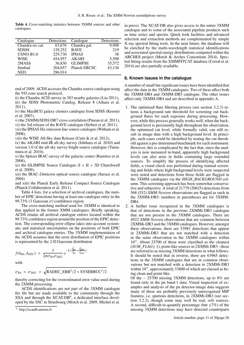
Table 4. Cross-matching statistics between 3XMM sources and othercatalogues.
Catalogue Detections Catalogue DetectionsChandra src cat. 63,676 Chandra gal. 9,908SDSS8 129,252 RAVE 219USNO-B1.0 229,730 IPHAS 38WISE 454,957 AKARI 5,5982MASS 36,830 GLIMPSE 35,572Simbad 204,657 Planck ERCSC 43,136NED 296,914
end of 2009. ACDS accesses the Chandra source catalogue usingthe VO cone search protocol,ii) the Chandra ACIS survey in 383 nearby galaxies (Liu 2011),iii) the SDSS Photometric Catalog, Release 8 (Aihara et al.2011),iv) the MaxBCG galaxy clusters catalogue from SDSS (Koesteret al. 2007),v) the 2XMMi/SDSS DR7 cross-correlation (Pineau et al. 2011),vi) the 3rd release of the RAVE catalogue (Siebert et al. 2011),vii) the IPHAS Hα emission line source catalogue (Witham et al.2008),viii) the WISE All-Sky data Release (Cutri & et al. 2012),ix) the AKARI mid-IR all-sky survey (Ishihara et al. 2010) andversion 1.0 of the all-sky survey bright source catalogue (Yama-mura et al. 2010),x) the Spitzer IRAC survey of the galactic center (Ramírez et al.2008),xi) the GLIMPSE Source Catalogue (I + II + 3D Churchwellet al. 2009),xii) the IRAC-24micron optical source catalogue (Surace et al.2004)and xiii) the Planck Early Release Compact Source Catalogue(Planck Collaboration et al. 2011).
Table 4 lists, for a selection of archival catalogues, the num-ber of EPIC detections having at least one catalogue entry in the99.73% (3 Gaussian σ) confidence region.
The cross-matching method used for 3XMM is identical tothat applied in the former XMM catalogues. Briefly speaking,ACDS retains all archival catalogue entries located within the99.73% confidence region around the position of the EPIC detec-tion. The corresponding error ellipse takes into account system-atic and statistical uncertainties on the positions of both EPICand archival catalogue entries. The 3XMM implementation ofthe ACDS assumes that the error distribution of EPIC positionsis represented by the 2-D Gaussian distribution
f (δRA, δDEC) =1
2πσRAσDEC
e− 1
2 (δ2RA
σ2RA
+δ2DEC
σ2DEC
))
with
σRA = σDEC =
√
RADEC_ERR2/2 + SYSERRCC2/2
thereby correcting for the overestimated error value used duringthe 2XMM processing.
ACDS identifications are not part of the 3XMM cataloguefits file but are made available to the community through theXSA and through the XCAT-DB6, a dedicated interface devel-oped by the SSC in Strasbourg (Motch et al. 2009, Michel et al.
6 http://xcatdb.unistra.fr
in press). The XCAT-DB also gives access to the entire 3XMMcatalogue and to some of the associated pipeline products suchas time series and spectra. Quick look facilities and advancedselection and extraction methods are complemented by simpleX-ray spectral fitting tools. In the near future, the database willbe enriched by the multi-wavelength statistical identificationsand associated spectral energy distributions computed within theARCHES project (Motch & Arches Consortium 2014). Spec-tral fitting results from the XMMFITCAT database (Corral et al.2014) are also partially available.
8. Known issues in the catalogue
A number of small but significant issues have been identified thataffect the data in the 3XMM catalogues. Two of these affect boththe 3XMM-DR4 and 3XMM-DR5 catalogue. The other issuesaffect only 3XMM-DR4 and are described in appendix A.
1. The optimised flare filtering process (see section 3.2.3) re-turns a background rate threshold for screening out back-ground flares for each exposure during processing. How-ever, while this process generally works well, when the back-ground level is persistently high throughout the observation,the optimised cut level, while formally valid, can still re-sult in image data with a high background level. In princi-ple, such cases could be identified by testing the cut thresh-old against a pre-determined benchmark for each instrument.However, this is complicated by the fact that, since the anal-ysis is now measured in-band, apparently high backgroundlevels can also arise in fields containing large extendedsources. To simplify the process of identifying affectedfields, a visual check was performed during manual screen-ing and fields where high background levels were suspectedwere noted and detections from those fields are flagged inthe 3XMM catalogues via the HIGH_BACKGROUND col-umn. This screening approach has been somewhat conserva-tive and subjective. A total of 21779 (20625) detections from568 (552) XMM-Newton observations are flagged as such inthe 3XMM-DR5: numbers in parentheses are for 3XMM-DR4.
2. A further issue recognized in the 3XMM catalogues isthat of detections in the previous 2XMMi-DR3 cataloguethat are not present in the 3XMM catalogues. There are4922 XMM-Newton observations that are common between2XMMi-DR3 and the 3XMM catalogues. However, amongstthese observations, there are 53981 detections that appearin 2XMMi-DR3 that are not matched with a detectionin the same observation in the 3XMM catalogues within10′′. About 25700 of these were classified as the cleanest(SUM_FLAG≤ 1), point-like sources in 2XMMi-DR3 - theseare referred to as missing 3XMM detections in what follows.It should be noted that in reverse, there are 63965 detec-tions in the 3XMM catalogues that are in common obser-vations but not matched with a detection in 2XMMi-DR3within 10′′, approximately 33600 of which are classed as be-ing clean and point-like.Of the ∼ 25700 missing 3XMM detections, up to 8% arefound only in the pn band-1 data. Visual inspection of ex-amples and analysis of the pn detector-image data suggestsmany of these are probably previously unrecognised MIPfeatures, i.e. spurious detections, in 2XMMi-DR3 (see sec-tion 3.2.2), though some may well be real, soft sources.A second, difficult-to-quantify percentage (but ≤7%) of themissing 3XMM detections may have detected counterparts
Article number, page 11 of 20page.20

A&A proofs: manuscript no. 3XMM_v10
in the 3XMM catalogues but be unmatched within 10′′ dueto imperfect astrometry in either the 2XMMi-DR3 and/or3XMM catalogue. A third component of up to around3% of the missing 3XMM detections may be detectionsin 2XMMi-DR3 that are associated with hitherto unrecog-nised/unflagged detector features - such features become ap-parent when the missing 3XMM detections are plotted in de-tector coordinates for each EPIC instrument, after allowingfor likely real detections in the same regions that are detectedin more than 1 instrument.Other explanations for the missing 3XMM detections in-clude– A small number (<1%) are pairs of visually verified close
sources that were separated in 2XMMi-DR3 but foundas either a single extended or a single unresolved pointsource in 3XMM.
– A small number of cases are likely spurious detectionsin the wings of bright sources in 2XMMi-DR3 that wereerroneously unflagged during the manual screening pro-cess for 2XMMi-DR3 and were not detected in 3XMM.
Nevertheless, the above-mentioned explanations account foronly a modest fraction (≤20%) of all the clean, point-like missing 3XMM detections. Some 75% of the missing3XMM detections have EPIC likelihoods in 2XMMi-DR3,L, < 10 (90% have L < 15). It might be thought that themissing 3XMM detections could arise from spurious detec-tions due to random statistical background fluctuations (falsepositives) in 2XMMi-DR3 - the numbers of such detections,estimated from simulations, was discussed in in section 9.4of Watson et al. (2009). However, this is not so because al-though there are notable changes to the pipeline processingbetween the 2XMMi-DR3 and 3XMM catalogues, the inputODFs and associated event data are generally the same forthe common observations, i.e. the data are not independent.As such, the cause of the majority of the missing 3XMMdetections remains unclear. However, in comparing 3XMMagainst 2XMMi-DR3, we need to acknowledge the changesin processing. In particular, the changes to the flare filtering(see section 3.2.3) can result in subtle changes to the back-ground spline model which can impact on the measured de-tection likelihood of sources. It is likely these changes areat least partly responsible for the numbers of 2XMMi-DR3detections not found in 3XMM. It should be noted that moredetections appear in 3XMM that are not found in commonobservations in 2XMMi-DR3 - the cause is likely to be sim-ilar, with extra objects being found due to the enhancementsin sensitivity afforded in the 3XMM catalogues.
9. Catalogue characterisation
9.1. General properties
The 3XMM-DR5 catalogue contains 565962 (531261) detec-tions, associated with 396910 (372728) unique sources on thesky, extracted from 7781 (7427) public XMM-Newton observa-tions - numbers in parentheses are for 3XMM-DR4. Amongstthese, 70453 (66728) unique sources have multiple detections,the maximum number of repeat detections being 48 (44 for3XMM-DR4), see fig. 4. 55640 X-ray detections in 3XMM-DR5are identified as extended objects, i.e. with a core radius param-eter, rcore, as defined in section 4.4.4 of Watson et al. (2009),> 6′′, with 52493 of these having rcore < 80′′. Overall proper-ties in terms of completeness and false detection rates are not
Fig. 4. Numbers of 3XMM-DR5 unique sources comprising given num-bers of repeat detections.
expected to differ significantly from those described in Watsonet al. (2009).
9.2. Astrometric properties
As outlined in section 3.4, several changes have been made to theprocessing that affect the astrometry of the 3XMM cataloguesrelative to previous XMM-Newton X-ray source catalogues. Toassess the quality of the current astrometry, we have broadlyfollowed the approach outlined in Watson et al. (2009). Detec-tions in the 3XMM-DR5 catalogue were cross-correlated againstthe Sloan Digital Sky Survey (SDSS) DR12Q quasar catalogue(Paris et al. in prep.), which contains ∼297300 objects spec-troscopically classified as quasars - positions and errors weretaken from the SDSS DR9 catalogue. X-ray detections withan SDSS quasar counterpart within 15′′ were extracted. Point-like 3XMM-DR5 detections were selected with summary flag 0,from successfully catcorr-corrected fields, with EPIC detectionlog-likelihood>8 and at off-axis angles< 13′. The SDSS quasarswere required to have warning flag 0, morphology 0 (point-like)and r’ and g’ magnitudes both <22.0. This yielded a total of 66143XMM-QSO pairs. In the 13 cases where more than one opticalquasar match was found within 15′′, the nearest match was re-tained.
The cross-matching used the catcorr-corrected RA and DECX-ray detection coordinates. The measured separation, ∆r,and the overall 1-dimensional XMM position error, σ1D (=σpos/
√2), were recorded. Hereσpos is the radial positional error,
POSERR, in the catalogues, which is the quadrature sum of theXMM positional uncertainties resolved in the RA and DEC di-rections. As noted by Watson et al. (2009), if the offsets of the X-ray sources and their SDSS quasar counterparts are normalisedby the total position error, the distribution of these normalisedoffsets is expected to follow the Rayleigh distribution,
N(x)dx ∝ xe−x2/2dx (7)
where x = ∆r/σtot - errors on the SDSS quasar posi-tions were included though they are generally ≤ 0.1′′, muchsmaller than the vast majority ofσ1D values in 3XMM-DR5. The
Article number, page 12 of 20page.20
S. R. Rosen et al.: The XMM-Newton serendipitous survey
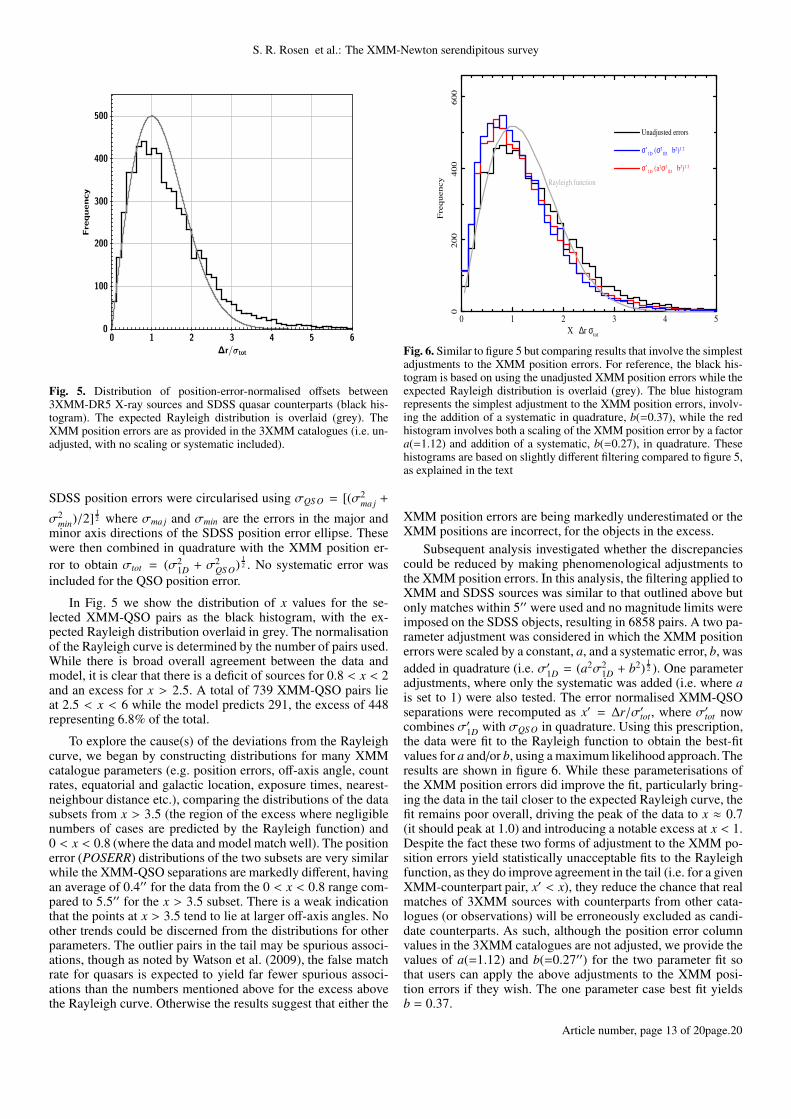
Fig. 5. Distribution of position-error-normalised offsets between3XMM-DR5 X-ray sources and SDSS quasar counterparts (black his-togram). The expected Rayleigh distribution is overlaid (grey). TheXMM position errors are as provided in the 3XMM catalogues (i.e. un-adjusted, with no scaling or systematic included).
SDSS position errors were circularised using σQS O = [(σ2ma j+
σ2min
)/2]12 where σma j and σmin are the errors in the major and
minor axis directions of the SDSS position error ellipse. Thesewere then combined in quadrature with the XMM position er-ror to obtain σtot = (σ2
1D+ σ2
QS O)
12 . No systematic error was
included for the QSO position error.
In Fig. 5 we show the distribution of x values for the se-lected XMM-QSO pairs as the black histogram, with the ex-pected Rayleigh distribution overlaid in grey. The normalisationof the Rayleigh curve is determined by the number of pairs used.While there is broad overall agreement between the data andmodel, it is clear that there is a deficit of sources for 0.8 < x < 2and an excess for x > 2.5. A total of 739 XMM-QSO pairs lieat 2.5 < x < 6 while the model predicts 291, the excess of 448representing 6.8% of the total.
To explore the cause(s) of the deviations from the Rayleighcurve, we began by constructing distributions for many XMMcatalogue parameters (e.g. position errors, off-axis angle, countrates, equatorial and galactic location, exposure times, nearest-neighbour distance etc.), comparing the distributions of the datasubsets from x > 3.5 (the region of the excess where negligiblenumbers of cases are predicted by the Rayleigh function) and0 < x < 0.8 (where the data and model match well). The positionerror (POSERR) distributions of the two subsets are very similarwhile the XMM-QSO separations are markedly different, havingan average of 0.4′′ for the data from the 0 < x < 0.8 range com-pared to 5.5′′ for the x > 3.5 subset. There is a weak indicationthat the points at x > 3.5 tend to lie at larger off-axis angles. Noother trends could be discerned from the distributions for otherparameters. The outlier pairs in the tail may be spurious associ-ations, though as noted by Watson et al. (2009), the false matchrate for quasars is expected to yield far fewer spurious associ-ations than the numbers mentioned above for the excess abovethe Rayleigh curve. Otherwise the results suggest that either the
0 1 2 3 4 5
02
00
40
06
00
Fre
qu
en
cy
X = ∆r/σtot
Unadjusted errors
σ’1D
=(a2σ21D
+ b2)1/2
Rayleigh function
σ’1D
=(σ21D
+ b2)1/2
Fig. 6. Similar to figure 5 but comparing results that involve the simplestadjustments to the XMM position errors. For reference, the black his-togram is based on using the unadjusted XMM position errors while theexpected Rayleigh distribution is overlaid (grey). The blue histogramrepresents the simplest adjustment to the XMM position errors, involv-ing the addition of a systematic in quadrature, b(=0.37), while the redhistogram involves both a scaling of the XMM position error by a factora(=1.12) and addition of a systematic, b(=0.27), in quadrature. Thesehistograms are based on slightly different filtering compared to figure 5,as explained in the text
XMM position errors are being markedly underestimated or theXMM positions are incorrect, for the objects in the excess.
Subsequent analysis investigated whether the discrepanciescould be reduced by making phenomenological adjustments tothe XMM position errors. In this analysis, the filtering applied toXMM and SDSS sources was similar to that outlined above butonly matches within 5′′ were used and no magnitude limits wereimposed on the SDSS objects, resulting in 6858 pairs. A two pa-rameter adjustment was considered in which the XMM positionerrors were scaled by a constant, a, and a systematic error, b, wasadded in quadrature (i.e. σ′1D
= (a2σ21D+ b2)
12 ). One parameter
adjustments, where only the systematic was added (i.e. where ais set to 1) were also tested. The error normalised XMM-QSOseparations were recomputed as x′ = ∆r/σ′tot, where σ′tot nowcombines σ′1D
with σQS O in quadrature. Using this prescription,the data were fit to the Rayleigh function to obtain the best-fitvalues for a and/or b, using a maximum likelihood approach. Theresults are shown in figure 6. While these parameterisations ofthe XMM position errors did improve the fit, particularly bring-ing the data in the tail closer to the expected Rayleigh curve, thefit remains poor overall, driving the peak of the data to x ≈ 0.7(it should peak at 1.0) and introducing a notable excess at x < 1.Despite the fact these two forms of adjustment to the XMM po-sition errors yield statistically unacceptable fits to the Rayleighfunction, as they do improve agreement in the tail (i.e. for a givenXMM-counterpart pair, x′ < x), they reduce the chance that realmatches of 3XMM sources with counterparts from other cata-logues (or observations) will be erroneously excluded as candi-date counterparts. As such, although the position error columnvalues in the 3XMM catalogues are not adjusted, we provide thevalues of a(=1.12) and b(=0.27′′) for the two parameter fit sothat users can apply the above adjustments to the XMM posi-tion errors if they wish. The one parameter case best fit yieldsb = 0.37.
Article number, page 13 of 20page.20

A&A proofs: manuscript no. 3XMM_v10
Other tests involved (i) imposing a lower bound on the XMMposition error (σ′1D
= max(σ1D, σmin)) and (ii) including an off-axis-dependent systematic involving a scalar, c, (σ′21D
= σ21D+
c2Θ2) where Θ is the off-axis angle. These latter modificationsprovide slightly better matches to the Rayleigh curve but stilldrive the peak of the data to x ≈ 0.7, again creating an excess atx < 1. A further test in which the XMM position error is definedas σ′1D
= σ1D for x < xt and σ′21D= σ2
1D+ d2(x − xt)2 for x ≥ xt
(where d is a simple scalar and xt is a threshold value in x) doesyield a marked enhancement in the likelihood for the fit but inthis case, the data undershoot the Rayleigh curve at x > 2 andexceed it at 0.6 < x < 2.
We conclude that while the more complex adjustments to theXMM position errors can formally improve the match betweenthe error-normalised XMM-QSO separations and the Rayleighcurve, none provides a statistically acceptable match. Moreover,the cases that yield the best improvements in the fit likelihoodhave no compelling technical rationale.
One possible scenario that might explain the discrepancies iswhere, in a subset of XMM observations, the catcorr task obtainsan incorrect solution for the frame rectification. This could man-ifest itself as erroneous translational (RA/DEC) and/or rotationalcorrections. A number of XMM fields that contain XMM-QSOpairs from the excess at x > 3.5 also contain significant numbersof other XMM-QSO pairs that lie at x < 3. If such erroneous rec-tification corrections were present, we would expect many otherpairs in the field to be shifted to larger x values and/or to havea dependence on the off-axis angle (if the rotational correctionis wrong). That this is not evident in example fields examinedindicates incorrect frame rectification is unlikely to be the un-derlying cause.
9.3. Background flare filtering
As noted in section 3.2.3, an optimisation algorithm was adoptedto determine the count rate threshold for defining the flare GTIs.This process was employed to maximise sensitivity to source de-tection and can come at the expense of reduced exposure time.Often, the new process results in GTIs that are similar to thosederived from the fixed threshold cuts used in pre-cat9.0 pipelineprocessing. However, in some cases, significant improvementscan be obtained in sensitivity.
Of particular interest are cases where the background risesor falls slowly. In such cases, allowing a modest increase in thebackground count rate can yield a marked increase in exposuretime, resulting in a significant improvement in the sensitivity tothe detection of faint sources. A good example of this is illus-trated in figure 7. As is evident from the light curves, the op-timised cut threshold includes significantly more exposure timefor a very modest increase in background level, producing a fac-tor 5.5 increase in the harvest of detected sources.
Another aspect of the optimised flare filtering approach isthat the increase in exposure time can result in exposures beingused that were previously rejected in processing with pre-cat9.0pipelines.
The pre-cat9.0 and cat9.0 light curves in figure 7 also high-light the fact that the change of energy band used can yield somesignificant differences in the strengths and even shapes of flarefeatures in the data.
The implementation of the optimised flare filtering approachwas done in conjunction with some of the other upgrades, suchas the use of the empirical PSF (see section 3.3). As such, wehave not directly isolated the impacts on source detection of the
01 2 5 11 23 47 93 188 375 748
Fig. 7. An example of the improvement offered by the optimised back-ground flare filtering algorithm. Top panels: Left: high-energy MOS1background flare light curve created by the pre-cat9.0 pipeline, used forthe 2XMMi-DR3 catalogue - the red line is the fixed (2 cts/s/arcmin2)count rate cut threshold applied. Right: in-band (0.5-7.5 keV) lightcurve used in the cat-9.0 pipeline used for 3XMM-DR4 and 3XMM-DR5 - the red line shows the optimised cut rate threshold derived forthe light curve. The lower panels show the resulting, corresponding(smoothed) images, after filtering out the data above the respective rate-cut thresholds. Sources found by the source detection algorithm are in-dicated by red circles.
optimised flare filtering process alone. Nevertheless, compari-son of the numbers of source detections between the set of 4922observations that are common to the 2XMMi-DR3 and 3XMM-DR5 catalogues, indicates a net increase of 10047 detections in3XMM-DR5, i.e. a 2.9% increase.
9.4. Extraction of spectral and time series products
As described in section 4.1, spectra and time series of detec-tions are now extracted using optimised extraction apertures thatare intended to maximise the overall S/N of the resulting prod-uct. To assess this, spectra were re-extracted for all detectionsand exposures for which spectra were produced during the bulkreprocessing, using a circular aperture of fixed radius (28′′) ineach case, centred at the same location as the detection posi-tion used during the bulk reprocessing. Other than the changeof aperture radius, processing was essentially identical to thatused in the bulk reprocessing. The S/N, S , of each spectrum wasthen computed as S = Cs/CT
12 . Here Cs = CT − Cb, where CT
is the total number of counts measured in the spectrum from thesource aperture, Cs is the number of counts from the source in thesource aperture and Cb is the number of background counts in thesource aperture, the latter being estimated from the total countsin the background region, scaled by the ratio of source and back-ground region areas. Counts included in this analysis were drawnfrom PHA channels with quality< 5 (in XSPEC terms). The S/Nwas computed in this way for the spectra from the optimised andfixed apertures - the spectral data used for background subtrac-tion were taken from the same background spectrum (from the
Article number, page 14 of 20page.20

S. R. Rosen et al.: The XMM-Newton serendipitous survey
Fig. 8. log10(S o/S f ) plotted against the log of the total counts, CT , mea-sured from the optimised aperture. The grey points indicate the data andinclude only clean (SUM_FLAG=0), point-like (EP_EXTENT =0) de-tections. The red line links measurements of the average log10(S o/S f ),in bins sampling the range in CT , for cases where −1 < log10(S o/S f ) <1. The blue line is similar but is for the subset of data where, addi-tionally, the background rate is > 10−8 cts s−1 (sub-pixel)−2 (sub-pixelshave side lengths of 0.05 ′′). The lower X-axis limit reflects the mini-mum threshold of 100 total counts in the optimised extraction aperture,imposed for extracting XMM source spectra; the plot is otherwise trun-cated for clarity.
bulk reprocessing) in each case and the background counts usedwere drawn only from the same channels as used for the sourcecounts.
In Figure 8 the log of the ratio of the S/N values from thespectra extracted from the optimised (S o) and fixed (S f ) aper-tures, i.e. log10(S o/S f ), is plotted against log(CT ) from the opti-mised aperture, for MOS1 spectra. Only spectra from the clean-est (SUM_FLAG=0), point-like (EP_EXTENT=0) detections areincluded.
It is evident from the positive asymmetry aboutlog10(S o/S f ) = 0, that the optimisation procedure doesimprove the S/N of the spectra, especially for spectra with lower(CT < 500) numbers of extracted counts, as expected. Overall,67.5% of the MOS1 spectra with 100 < CT < 50000 cts (within−1 < log10(S o/S f ) < 1 which excludes 21 positive outliers)have higher S/N in the optimised aperture than those extractedfrom the fixed apertures. The red line in figure 8 shows theaverage of log10(S o/S f ) of all the data as a function of CT andindicates that spectra extracted from the optimised apertureswith CT = 100 cts have, on average, S/N values 12% higherthan those extracted in the fixed apertures. It is anticipatedthat sources detected in fields with high background levelswould benefit from the optimisation procedure. Indeed the blueline in figure 8, which reflects the subset of detections whosebackground levels are above 10−8 cts s−1 (sub-pixel)−2 (i.e.amongst the highest 15% of background levels), demonstratesthis - spectra of such detections extracted from optimisedapertures with CT = 100 cts, have average S/N values 39%higher than the spectra from the corresponding fixed apertures.
Fig. 10. Histogram of the logarithm of the ratio of extensions betweenthe best observation and the other observations of the same source, nor-malised by the error. The solid red line is the best Gaussian fit to thehistogram. The dashed red line is the expected mean (0).
9.5. Extended sources
The detection and characterisation of extended sources for3XMM was performed as in 2XMM (Watson et al. 2009). Thecaveats listed in section 9.9 of that paper still apply to 3XMM.However the better representation of the PSF has helped to im-prove extended source detection and characterisation. Many ex-tended sources with SC_SUM_FLAG = 4 in 2XMM now haveSC_SUM_FLAG = 3 in 3XMM, indicating that the region isstill complex but the detection itself is unlikely to be spurious.We have also looked at the distribution of extension likelihoodvs. flux as in Fig. 15 of Watson et al. (2009). Fig. 9 shows that3XMM considers many bright extended sources to be reliable(SC_SUM_FLAG < 2) whereas in 2XMM most of them hadhigher flag values indicating more significant issues with the dataquality.
We have complemented this study by inter-comparing the3XMM (DR4) results when a source was observed more thanonce, and with an independent serendipitous search for clus-ters of galaxies. We restricted the comparison to the best-qualitysources with SC_SUM_FLAG = 0. In 3XMM-DR4, 667 sourceshave been observed several times as extended, each observa-tion being processed independently. We define as the “referencevalue” the extension (EP_EXTENT) associated to the detectionwith the highest likelihood value (EP_8_DET_ML column). Weinvestigated the agreement of the extension parameter betweenthe “reference" and the other observations of the same source.We ignored observations when a given source was not detectedas extended (mostly because of insufficient exposure) or whenthe extension was set to 80′′ (maximum value allowed in the fit).
In Fig. 10 we show the distribution (in log space) of theratio between the “reference” extension Extre f and the cur-rent one Extcur, normalised by the corresponding error equalto
√
(σre f /Extre f )2 + (σcur/Extcur)2, whereσre f andσcur are theextension errors for the “reference” and current observation re-spectively. We fit the histogram result by a Gaussian function,obtaining a mean value equal to 0.512 (in σ units) with a stan-
Article number, page 15 of 20page.20

A&A proofs: manuscript no. 3XMM_v10
Fig. 9. Distribution of total flux and extension likelihood of all extended sources with SC_SUM_FLAG < 2, in the 2XMM (left) and 3XMM (right)catalogues.
Fig. 11. Comparison of the ratio of extensions and the ratio of countrates obtained by the 3XMM and the XCLASS catalogues. The red solidline is the relation 1:1.
dard deviation equal to 1.943 (we would expect a mean of 0 anda standard deviation of 1 for random fluctuations). We concludethat there exists an additional scatter larger than statistical (of un-known origin) and that the reference observation, which is alsothe deepest one, estimates a larger extension on average.
The XCLASS catalogue is based on the analysis of archivalobservations from the XMM-Newton observatory. The XCLASSteam processed 2774 high Galactic latitude observations from
the XMM archive (as of 2010 May) and extracted a serendipi-tous catalogue of some 850 clusters of galaxies based on purelyX-ray criteria, following the methodology developed for theXMM Large Scale Survey (Pierre et al. 2007). We used the sub-sample of 422 galaxy clusters available online at http://xmm-lss.in2p3.fr:8080/l4sdb/ to compare the extension and the countrate obtained for the same sources from the two different pro-cedures (ie. the XCLASS and 3XMM processing). The analyticexpression used to represent extended sources in XCLASS wasthe same as in 3XMM (β-model with β=2/3) so the numbersshould be directly comparable. All 422 clusters are in 3XMM-DR4, but 59 (mostly faint or irregular objects) were classified aspoint sources.
For the 363 extended sources in common, we compared theextent and the count rate in the [0.5-2.0] keV band obtained by3XMM and XCLASS. We found that, for both quantities, the3XMM estimates seem to be biased low with respect to theXCLASS values. The best fit regression on source extent re-sulted in a slope of 0.7 (Ext3XMM ≃ 0.7ExtXCLAS S ). Excludingclear outliers (difference of extension larger than 20′′, typicallyvery faint sources or very bright sources affected by a strongpile-up) the slope increases to 0.85. We conclude that, even ex-cluding these extreme sources, there remains a bias of ≃ 15%between the extensions estimated by 3XMM and XCLASS.
There exists a similar (a little smaller) bias on the count rate.However Fig. 11 shows that there exists a close correlation be-tween both ratios, implying that only one parameter describesthe difference in extent and count rates and that, if the sourceextents were forced to agree, the count rates would agree too.There is no obvious way to know whether the 3XMM or theXCLASS estimate is better but, together with the inter-3XMMcomparison, this result indicates that the purely statistical exten-sion error underestimates the real error.
10. Examples
Thanks to the wide range of parameters provided in the cata-logue, sources matching specific criteria can be isolated (for ex-
Article number, page 16 of 20page.20

S. R. Rosen et al.: The XMM-Newton serendipitous survey
ample variability criteria of X-ray hardness ratios). In this sec-tion we show some examples of lightcurves (Fig. 12) and spec-tra (Fig. 13) extracted from the different EPIC cameras. Theplots shown are those associated with the on-line catalogue. Bothknown and new sources are presented. It is immediately obviousfrom the two Figures that objects with extremely diverse charac-teristics are found. Variability on very different timescales is seenin Fig. 12, showing short and long flares, slow rises and steadydeclines in count rate as well as deep eclipses. From visual ex-amination of the strong variability in Fig. 12c, it was quickly ob-vious that this new X-ray source was a polar (Webb et al. to besubmitted). Fig. 12e shows a strong decline in flux, which, whencoupled with the hard spectrum observed for this source, sug-gests that this might be a previously unknown orphan gamma-ray afterglow.
The spectra shown in Fig. 13 are also very varied and origi-nate from a variety of astrophysical objects, ranging from stars,compact objects, galaxies and clusters of galaxies. An unidenti-fied X-ray source is included in Fig. 13a, which also has a highlyvariable lightcurve, showing a steady decline in count rate, butwith a strong flare superposed. The nature of this source is notobvious and more work will be needed to identify its nature. Thesources in the full 3XMM catalogue are of course dominated byunidentified objects, emphasising the large discovery space pro-vided by the catalogue.
11. Catalogue access
The catalogue is provided in several formats. Firstly, a Flexi-ble Image Transport System (FITS) file and a comma-separatedvalues (CSV) file is provided containing all of the detectionsin the catalogue. For 3XMM-DR5 there are 565962 rows and323 columns. A separate version of the catalogue (the slim cat-alogue) is also provided that contains only the unique sources,i.e. 396910 rows, and has 44 columns, essentially those con-taining information about the unique sources. This catalogue isalso provided in FITS and CSV format. Ancillary tables to thecatalogue also available from the XMM-Newton Survey ScienceCentre webpages7 include the table of observations incorporatedin the catalogue and the target identification and classificationtable.
The XMM-Newton Survey Science Centre webpages provideaccess to the 3XMM catalogue, as well as links to the differentservers distributing the full range of catalogue products. Theseinclude, the XMM-Newton XSA, which provides access to all ofthe 3XMM data products, and the ODF data, the XCat-DB8 pro-duced and maintained by the XMM-Newton SSC, which containspossible EPIC source identification produced by the pipeline byquerying 228 archival catalogues. Finding charts are also pro-vided for these possible identifications. Other source propertiesas well as images, time series, spectra, fit results from the XMM-FITCAT are also provided. Multi-wavelength data taken as apart of the XID (X-ray identification project) run by the SSCover the first fifteen years of the mission are also provided inthe XIDresult database9. The LEDAS server10 provides anotherway to access the 3XMM catalogue and its products, whilst thethe upper limit server11 allows the user to specify a sky positionand obtain upper limits on the EPIC fluxes of a point source at
7 http://xmmssc.irap.omp.eu/8 http://xcatdb.unistra.fr/3xmm/9 http://xcatdb.unistra.fr/xidresult/
10 http://www.ledas.ac.uk/arnie5/arnie5.php?action=basic&catname=3xmm11 http://www.ledas.ac.uk/flix/flix.html
the position if the location has been observed by XMM-Newtonbut no source was detected. The catalogue can also be accessedthrough HEASARC12 and VIZIER13. The results of the exter-nal catalogue cross-correlation carried out for the 3XMM cata-logue (section 7) are available as data products within the XSAand LEDAS or through the XCat-DB. The XMM-Newton SurveyScience Centre webpages also detail how to provide feedback onthe catalogue.
Where the 3XMM catalogues are used for research andpublications, please acknowledge their use by citing this paperand including the following:
This research has made use of data obtained from the 3XMMXMM-Newton serendipitous source catalogue compiled by the10 institutes of the XMM-Newton Survey Science Centre se-lected by ESA.
12. Future catalogue updates
Incremental releases (data releases) are planned to augment the3XMM catalogue. An additional year of data will be includedwith each data release. Data release 6 (DR6) will provide databecoming public during 2014 and should be released by the endof 2015. These catalogues will be accessible as described in Sec-tion 11.
13. Summary
This paper presents the third major release of the XMM-Newtonserendipitous source catalogue (3XMM), in its original version(3XMM-DR4) and in the first incremental version (3XMM-DR5). The 3XMM catalogues have been constructed by theXMM-Newton Survey Science Centre and the 3XMM-DR5 cata-logue becomes the largest catalogue of X-ray sources detectedusing a single X-ray observatory. The characteristics and im-provements of this catalogue, with respect to previous versions,are outlined as well as how to cite and access the catalogue. Thispaper serves as the reference for future incremental versions ofthe same catalogue (3XMM-DR6, etc), as new XMM-Newtondata becomes publicly available.
Acknowledgements. Firstly, we are extremely grateful for the strong support pro-vided by the XMM-Newton SOC. We also thank the CDS team for their ac-tive contribution and support. The French teams are grateful to Centre Nationald’Études Spatiales CNES for their outstanding support for the SSC activities.The German teams are grateful to the Deutsches Zentrum für Luft- und Raum-fahrt for supporting this activity under grants 50 OX 1101, 50 OX 1401 and50 OG 1101. The University of Leicester acknowledges the financial support ofthe UK Space Agency and also ESA. FJC acknowledges financial support bythe Spanish Ministry of Economy and Competitiveness through grant AYA2012-31447. MTC acknowledges financial support from the Spanish Ministry of Sci-ence and Innovation through grant AYA2010-21490-C02-1. The Italian team ac-knowledges financial support during the years from the Ministero dell’Istruzione,dell’Universita’ e della Ricerca (MIUR), from the Agenzia Spaziale Italiana(ASI) and from the Istituto Nazionale di Astrofisica (INAF). This research hasalso made use of the SIMBAD database, of the VizieR catalogue access tool,and of Aladin, operated at CDS, Strasbourg, France, the TOPCAT/Stilts soft-ware written by Mark Taylor of the University of Bristol, UK and the NASAHEASARC FTOOLS package14 (Blackburn 1995).
12 http://heasarc.gsfc.nasa.gov/db-perl/W3Browse/w3table.pl?tablehead=name%313 http://vizier.u-strasbg.fr/cgi-bin/VizieR14 http://heasarc.gsfc.nasa.gov/ftools/
Article number, page 17 of 20page.20

A&A proofs: manuscript no. 3XMM_v10
Fig. 12. Example lightcurves taken directly from the 3XMM catalogue. a) 3XMM J111146.1-762010 = CHX 18N – T Tau-type star showing ashort flare b) 3XMM J000619.5+201210, A Seyfert 1, Markarian 335. c) 3XMM J184916.1+652943, a new 1.6 hour polar (Webb et al. to besubmitted). d) A 2MASS star (2MASS J00025638-3004447) showing two large flares. e) 3XMM J002159.4+614254, a new X-ray object showinga strong decline in flux. Possibly a gamma-ray burst afterglow. f) 3XMM J013334.0+303211, a high mass X-ray binary in M 33, M33 X-7,showing a 12.5 hour eclipse - the first eclipsing stellar-mass black hole binary discovered (Pietsch et al. 2006)
Appendix A: Known issues affecting 3XMM-DR4
only
– After the creation of the 3XMM-DR4 catalogue, it was dis-covered that the raw event files from the ODFs of a num-ber of mosaic mode sub-pointing observations containedcorrupted data whereby some of the events in a givensub-pointing ODF were actually from another sub-pointing.Since the raw event positions are specified in detector coordi-nates and are subsequently mapped to their sky locations dur-ing pipeline processing by reference to the observation bore-sight position, which is specified for the given sub-pointing,the celestial positions of these events are wrong and thereforeresults in some detections having incorrect celestial coordi-nates. The problem arose in the algorithm used to split theraw parent ODF into sub-pointing ODFs. In some cases allinstruments were affected while in others, only one or bothof the MOS instruments was affected. Of the 419 mosaic-mode sub-pointing observations included in 3XMM-DR4,82 are affected to some extent, involving 4918 detections.The affected observations are listed in the watchout section
of the XMMSSC 3XMM-DR4 catalogue web pages15. For3XMM-DR5, none of the affected mosaic sub-pointing ob-servations is included in the catalogue.
– The vignetting values provided in the 3XMM-DR4 catalogue(for each instrument, for bands 1 to 5) were found to havebeen computed for an energy of 0 keV rather than the en-ergy relevant to the band. Thus the values for each band ofa given instrument are identical. This error does not affectthe count rates or fluxes as the vignetting correction appliedto them is computed separately and has been verified as cor-rect. It is only the tabulated values in the vignetting columnsof the catalogue that are incorrect in 3XMM-DR4 and theyare correct in 3XMM-DR5.
– A significant issue identified after the public release of the3XMM-DR4 catalogue relates to the error values on var-ious quantities. It was established that the error quantities(i.e. columns containing an _ERR at the end) for the XIDband (band 9) count rates and fluxes of a significant num-ber (∼42200) of detections (∼10% of the catalogue) weresubstantially wrong (generally being overestimated by fac-tors up to ∼ 100 but in a few cases, up to 1000). A more
15 http://xmmssc-www.star.le.ac.uk/Catalogue/xcat_public_3XMM-DR4.html
Article number, page 18 of 20page.20
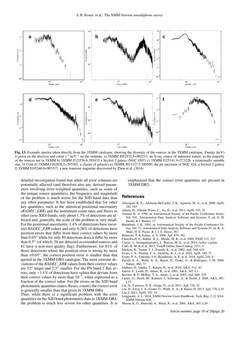
S. R. Rosen et al.: The XMM-Newton serendipitous survey
Fig. 13. Example spectra taken directly from the 3XMM catalogue, showing the diversity of the sources in the 3XMM catalogue. Energy (keV)is given on the abscissa and count s−1 keV−1 on the ordinate. a) 3XMM J052532.5+062533, an X-ray source of unknown nature, as the majorityof the sources are in 3XMM b) 3XMM J123536.6-395433 a Seyfert 2 galaxy (NGC 4507) c) 3XMM J125141.9+273226, a rotationally variablestar, 31 Com d) 3XMM J162838.2+393303, a cluster of galaxies e) 3XMM J011127.5-380500, the pn spectrum of NGC 424, a Seyfert 2 galaxyf) 3XMM J185246.6+003317, a new transient magnetar discovered by Zhou et al. (2014)
detailed investigation found that while all error columns arepotentially affected (and therefore also any derived param-eters involving error-weighted quantities, such as some ofthe unique source quantities), the frequency and magnitudeof the problem is much worse for the XID band data thanany other parameter. It has been established that for otherkey quantities, such as the statistical positional uncertainty(RADEC_ERR) and the instrument count rates and fluxes inother (non-XID) bands, only about 1.3% of detections are af-fected and, generally, the scale of the problem is very small.For the positional uncertainty, 1.4% of detections have incor-rect RADEC_ERR values and only 0.26% of detections haveposition errors that differ from their correct values by morethan 0.05′′ while for only 89 detections does it differ by morethan 0.5′′ (of which, 58 are detected as extended sources and81 have a non-zero quality flag). Furthermore, for 81% ofthose detections where the position error is wrong by morethan ±0.05′′, the correct position error is smaller than thatquoted in the 3XMM-DR4 catalogue. The most extreme de-viations of the RADEC_ERR values from their correct valuesare 32′′ larger and 2.3′′ smaller. For the PN band 2 flux er-rors, only ∼1.1% of detections have values that deviate fromtheir correct values by more than 10−5, when expressed as afraction of the correct value. For the errors on the XID bandphotometric quantities (rates, fluxes, counts) the correct erroris generally smaller than that given in 3XMM-DR4.Thus, while there is a significant problem with the errorquantities on the XID band photometric data in 3XMM-DR4,the problem is much less severe for other quantities. It is
emphasized that the correct error quantities are present in3XMM-DR5.
References
Abazajian, K. N., Adelman-McCarthy, J. K., Agüeros, M. A., et al. 2009, ApJS,182, 543
Aihara, H., Allende Prieto, C., An, D., et al. 2011, ApJS, 193, 29Arnaud, K. A. 1996, in Astronomical Society of the Pacific Conference Series,
Vol. 101, Astronomical Data Analysis Software and Systems V, ed. G. H.Jacoby & J. Barnes, 17
Blackburn, J. K. 1995, in Astronomical Society of the Pacific Conference Se-ries, Vol. 77, Astronomical Data Analysis Software and Systems IV, ed. R. A.Shaw, H. E. Payne, & J. J. E. Hayes, 367
Budavári, T. & Szalay, A. S. 2008, ApJ, 679, 301Churchwell, E., Babler, B. L., Meade, M. R., et al. 2009, PASP, 121, 213Corral, A., Georgantopoulos, I., Watson, M. G., et al. 2014, ArXiv e-printsCutri, R. M. & et al. 2012, VizieR Online Data Catalog, 2311, 0Edelson, R., Turner, T. J., Pounds, K., et al. 2002, ApJ, 568, 610Evans, I. N., Primini, F. A., Glotfelty, K. J., et al. 2010, ApJS, 189, 37Evans, P. A., Osborne, J. P., Beardmore, A. P., et al. 2014, ApJS, 210, 8Farrell, S. A., Webb, N. A., Barret, D., Godet, O., & Rodrigues, J. M. 2009,
Nature, 460, 73Ishihara, D., Onaka, T., Kataza, H., et al. 2010, A&A, 514, A1Jansen, F., Lumb, D., Altieri, B., et al. 2001, A&A, 365, L1Koester, B. P., McKay, T. A., Annis, J., et al. 2007, ApJ, 660, 239Lamer, G., Hoeft, M., Kohnert, J., Schwope, A., & Storm, J. 2008, A&A, 487,
L33Lin, D., Carrasco, E. R., Grupe, D., et al. 2011, ApJ, 738, 52Lin, D., Irwin, J. A., Godet, O., Webb, N. A., & Barret, D. 2013, ApJ, 776, L10Liu, J. 2011, ApJS, 192, 10Longinotti, A. L. 2014, XMM-Newton Users Handbook, Tech. Rep. 2.12, ESA:
XMM-Newton SOCMason, K. O., Breeveld, A., Much, R., et al. 2001, A&A, 365, L36
Article number, page 19 of 20page.20
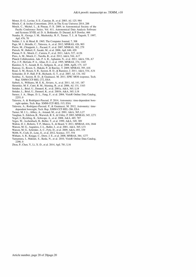
A&A proofs: manuscript no. 3XMM_v10
Monet, D. G., Levine, S. E., Canzian, B., et al. 2003, AJ, 125, 984Motch, C. & Arches Consortium. 2014, in The X-ray Universe 2014, 288Motch, C., Michel, L., & Pineau, F.-X. 2009, in Astronomical Society of the
Pacific Conference Series, Vol. 411, Astronomical Data Analysis Softwareand Systems XVIII, ed. D. A. Bohlender, D. Durand, & P. Dowler, 466
Nandra, K., George, I. M., Mushotzky, R. F., Turner, T. J., & Yaqoob, T. 1997,ApJ, 476, 70
Nelder, J. A. & Mead, R. 1965, The Computer Journal, 7, 308Page, M. J., Brindle, C., Talavera, A., et al. 2012, MNRAS, 426, 903Pierre, M., Chiappetti, L., Pacaud, F., et al. 2007, MNRAS, 382, 279Pietsch, W., Haberl, F., Sasaki, M., et al. 2006, ApJ, 646, 420Pineau, F.-X., Motch, C., Carrera, F., et al. 2011, A&A, 527, A126Pires, A. M., Motch, C., Turolla, R., et al. 2012, A&A, 544, A17Planck Collaboration, Ade, P. A. R., Aghanim, N., et al. 2011, A&A, 536, A7Pye, J. P., McGale, P. A., Allan, D. J., et al. 1995, MNRAS, 274, 1165Ramírez, S. V., Arendt, R. G., Sellgren, K., et al. 2008, ApJS, 175, 147Ramsay, G., Rosen, S., Hakala, P., & Barclay, T. 2009, MNRAS, 395, 416Read, A. M., Rosen, S. R., Saxton, R. D., & Ramirez, J. 2011, A&A, 534, A34Schneider, D. P., Hall, P. B., Richards, G. T., et al. 2007, AJ, 134, 102Sembay, S., Saxton, R. D., & Guainazzi, M. 2011, EPIC MOS response, Tech.
Rep. XMM-CCF-REL-272, ESASiebert, A., Williams, M. E. K., Siviero, A., et al. 2011, AJ, 141, 187Skrutskie, M. F., Cutri, R. M., Stiening, R., et al. 2006, AJ, 131, 1163Strüder, L., Briel, U., Dennerl, K., et al. 2001a, A&A, 365, L18Strüder, L., Briel, U., Dennerl, K., et al. 2001b, A&A, 365, L18Surace, J. A., Shupe, D. L., Fang, F., et al. 2004, VizieR Online Data Catalog,
2255, 0Talavera, A. & Rodríguez-Pascual, P. 2014, Astrometry: time-dependent bore-
sight update, Tech. Rep. XMM-CCF-REL-315, ESATalavera, A., Rodríguez-Pascual, P., & Guainazzi, M. 2012, Astrometry: time-
dependent boresight, Tech. Rep. XMM-CCF-REL-286, ESATurner, M. J. L., Abbey, A., Arnaud, M., et al. 2001, A&A, 365, L27Vaughan, S., Edelson, R., Warwick, R. S., & Uttley, P. 2003, MNRAS, 345, 1271Vogel, J., Byckling, K., Schwope, A., et al. 2008, A&A, 485, 787Voges, W., Aschenbach, B., Boller, T., et al. 1999, A&A, 349, 389Walton, D. J., Roberts, T. P., Mateos, S., & Heard, V. 2011, MNRAS, 416, 1844Watson, M. G., Auguères, J.-L., Ballet, J., et al. 2001, A&A, 365, L51Watson, M. G., Schröder, A. C., Fyfe, D., et al. 2009, A&A, 493, 339Webb, N., Cseh, D., Lenc, E., et al. 2012, Science, 337, 554Witham, A. R., Knigge, C., Drew, J. E., et al. 2008, MNRAS, 384, 1277Yamamura, I., Makiuti, S., Ikeda, N., et al. 2010, VizieR Online Data Catalog,
2298, 0Zhou, P., Chen, Y., Li, X.-D., et al. 2014, ApJ, 781, L16
Article number, page 20 of 20page.20