the yakima air wintertime nitrate study (yawns) final … · yakima air wintertime nitrate study...
TRANSCRIPT
The Yakima Air Wintertime Nitrate Study (YAWNS)
Final Report
Prepared by: Laboratory for Atmospheric Research
Department of Civil & Environmental Engineering Washington State University
2
Preface
The Laboratory for Atmospheric Research at Washington State University submits this Final Report as part of a contract project from the Washington Department of Ecology to conduct the Yakima Air Wintertime Nitrate Study (YAWNS). Contacts: Tim VanReken (Project PI and Lead Author) Laboratory for Atmospheric Research Department of Civil & Environmental Engineering Washington State University Phone: (509) 335-5055 Email: [email protected] Tom Jobson Laboratory for Atmospheric Research Department of Civil & Environmental Engineering Washington State University Phone: (509) 335-2692 Email: [email protected] Brian Lamb Laboratory for Atmospheric Research Department of Civil & Environmental Engineering Washington State University Phone: (509) 335-5702 Email: [email protected] Heping Liu Laboratory for Atmospheric Research Department of Civil & Environmental Engineering Washington State University Phone: (509) 335-1529 Email: [email protected] Susan Kaspari Department of Geology Central Washington University Phone: (509) 963-2738 Email: [email protected]
4
Executive Summary
The Yakima region in Washington is in attainment for the 24-hour PM2.5
Federal standard but monitored concentrations are frequently close to the standard,
primarily during winter, and a nonattainment classification has been considered a
possibility. At present, the primary strategy employed in Washington to reduce
PM2.5 during wintertime is to control the emissions from biomass burning, including
burning wood for home heating and outdoor burning of yard debris and orchard
tear-outs. The Washington Department of Ecology desired a more complete
understanding of the conditions that led to elevated PM2.5 levels in the Yakima
region; Yakima is unusual within Washington in that a significant fraction of the
wintertime PM2.5 is comprised of particulate nitrate. To understand the atmospheric
processes leading to elevated particulate nitrate, researchers at Washington State
University and Central Washington University were contracted to complete the
Yakima Air Wintertime Nitrate Study (YAWNS).
Observations for YAWNS were completed in the Yakima region during
January 2013. The primary measurement site was located in central Yakima on the
campus of Yakima Valley Community College. Measurements there included
meteorological conditions including surface mixing layer height and stability, trace
gas pollutants including CO, NOx, and VOCs, and the particle size distribution and
composition. A secondary site was located in Toppenish at the permanent
monitoring site operated by the Yakama Nation. YAWNS measurements at that site
included CO and NOx.
5
Several periods of elevated PM occurred during YAWNS. The analysis for this
report focused largely on two periods with a mesoscale stagnation episode lasting
for approximately two weeks in mid-January. During the Clear Sky period, from 10-
16 January, the diurnal cycle of the mixing layer followed a typical pattern. A
shallow stable surface layer overnight led to the elevated pollution, followed by
meteorologically driven dilution each afternoon. This Clear Sky period at night was
characterized by elevated levels of both primary (directly-emitted) and secondary
(produced chemically in the atmosphere) PM components, including nitrate.
The Clear Sky period was followed by a period of Persistent Cloud, which
lasted through 23 January. Unexpectedly, persistent low levels of all primary
pollutants, both trace gases and particulate material, characterized this period. Our
results indicate that this result was driven by the meteorology; the low-level cloud
enhanced surface mixing and increased dilution. However, concentrations of
secondary particulate material remained elevated, most notably particulate nitrate.
The elevated particulate nitrate concentrations found in Yakima during
winter are driven primarily by three factors: meteorology, and the availability of
ammonia and nitrate precursors. The wintertime meteorology of the region drives
gas-particle equilibrium of ammonium nitrate strongly toward the particle phase,
and high relative humidity conditions enhance this effect. High ammonia emissions
from agricultural sources in the area lead to elevated atmospheric concentrations,
which drives virtually all available nitric acid into the particulate phase, and results
in a condition where any additional nitric acid production would lead directly to
greater particulate nitrate levels. The production of particulate nitrate precursors is
6
complicated and sensitive to the varying meteorological and chemical conditions in
the valley. Given the presence of excess gaseous ammonia, there is almost always
sufficient reactive nitrogen available to produce elevated levels of particulate nitrate
if the right meteorological conditions take hold.
Little evidence was found that pollution in Yakima is significantly impacted
from regional transport via the Lower Yakima Valley. While meteorological
conditions and PM2.5 levels were typically similar at Yakima and Toppenish, the
analysis shows clearly that Yakima air quality is dominated by local sources. Though
of limited duration, it was found that the YAWNS study period was representative of
the typical wintertime meteorology and air quality conditions at Yakima.
Furthermore, the air quality in Yakima itself is consistent with other regional cities
with a similar mix of emissions sources. In general, when elevated ammonia
concentrations from agriculture mix with urban NOx emissions on humid winter
days, elevated particulate nitrate is common.
The YAWNS study has several implications for air quality management in
Washington State:
1. Ammonia emissions reductions are unlikely to result in significant
reductions in wintertime particulate nitrate unless order-of-magnitude
reductions are viable. As it stands, the ammonia levels in winter are high
enough that all available nitric acid is driven to particulate nitrate.
2. The pathway to reducing the available nitric acid / particulate nitrate pool is
not obvious. Particulate nitrate is the major atmospheric endpoint for NOx, so
7
NOx reductions would reduce the potential particulate nitrate pool. However,
NO also inhibits the formation of particulate nitrate by destroying the nitrate
radical, which is an important intermediate species. Therefore, it is possible
that local NOx reductions would drive the local atmospheric chemistry
toward increased particulate nitrate production. A numerical modeling effort
is required to determine the specific system behavior.
3. During persistent cloud conditions, mixing occurs throughout the cloud layer
and perhaps beyond, resulting in reduced levels of some pollutants, including
primary PM. While a reduction in the relative contribution of wood smoke to
organic PM is apparent during burn bans, calling or continuing burn bans
during persistent cloud conditions might be less critical than during clear sky
stagnation events. However, in addition to reducing exposure to the direct
wood smoke emissions, burn bans may also reduce exposure to secondary
organic aerosol.
4. The cloud-capped condition is linked to elevated secondary PM levels. Thus
the onset of cloud shifts the type of PM present, but elevated concentrations
would still be expected to be associated with the meteorological condition.
5. During YAWNS, burn bans appear to have been called at the correct times in
Yakima, especially during clear sky and mixed meteorological conditions. It
may be possible to adjust responses to anticipate the likely increased mixing
associated with persistent low-level cloud. While meteorological models do
not reliably predict such cloudy periods, once they set in they are clearly

8
identifiable. It may be possible to relax policy responses more confidently
when persistent cloud is accompanied by slight reductions in observed PM2.5
levels.

9
List of Abbreviations
AGL Above Ground Level
AIRPACT-4 Air Indicator Report for Public Awareness and Community Tracking- version 4
AMS Aerosol Mass Spectrometer
BBOA Biomass Burning Organic Aerosol
CMAQ Community Multi-Scale Air Quality (model)
CMU Carnegie Mellon University
CO Carbon monoxide
CO2 Carbon dioxide
CPC Condensation Particle Counter
CWU Central Washington University
DMA Differential Particle Analyzer
Dp Particle Diameter
EC Elemental Carbon
EI Emissions Inventory
elev. Elevation
EPA Environmental Protection Agency
EPCRA The Emergency Planning and Community Right-to-Know Act
equiv. Equivalent
est. Estimated
FEM Federal Equivalent Method
FRM Federal Reference Method
H2O Water
H3O+ Hydronium ion
HCHO Formaldehyde
HCO Formyl radical
HEPA High-efficiency particulate absorption (filter)
HNO3 Nitric acid
HO2 Hydroperoxyl radical
HOA Hydrocarbon-like Organic Aerosol
HONO Nitrous acid
10
HR High Resolution
HR-AMS High-Resolution Aerosol Mass Spectrometer
IMPROVE Interagency Monitoring of Protected Visual Environments (monitoring network)
Kp(T) Partitioning coefficient
Lat Latitude
Lon Longitude
lpm Liters per minute
M A generic molecule in a chemical reaction, typically nitrogen or oxygen in air
m/z Mass-to-charge ratio
MACL Mobile Atmospheric Chemistry Laboratory
meas. Measured
MOVES Motor Vehicle Emission Simulator
MS Mass Spectral
N2O5 Dinitrogen pentoxide
NEMA National Electrical Manufacturers Association
NH3 Ammonia
NH4+ Ammonium ion
(NH4)2SO4 Ammonium sulfate
NH4NO3 Ammonium nitrate
NIST National Institute of Standards and Technology
NO Nitric oxide
NO2 Nitrogen dioxide
NO3 Nitrate radical
NO3- Nitrate ion
NOAA National Oceanic and Atmospheric Administration
NOx Nitrogen oxides (the sum of NO and NO2)
NOy NOx plus the compounds that result from the oxidation of NOx
NOz The compounds that result from NOz oxidation (= NOy – NOx)
Ntot Total particle number concentration
O2 Oxygen
O3 Ozone
11
OH Hydroxl radical
OMC Organic Matter Carbon
OOA Oxidized Organic Aerosol
PAN Peroxy acytyl nitrate
PBL Planetary Boundary Layer
PFA Perfluoroalkoxy alkanes (polymer)
PM Particulate Mass
PM2.5 Fine Particulate Mass (particles smaller than 2.5 μm)
PMF Postive Matrix Factorization
ppbv Parts per billion by volume
ppmv Parts per million by volume
pptv Parts per trillion by volume
PSL Polystyrene latex (polymer)
PST Pacific Standard Time
PTOF Particle Time-of-Flight
PTR-MS Proton Transfer Reaction Mass Spectrometer
QA Quality Assurance
QC Quality Control
RCW Regulatory Code of Washington
RH Relative Humidity
SMPS Scanning Mobility Particle Sizer
SO42- Sulfate ion
SP2 Single Particle Soot Photometer
Td Townsend (unit of measure for the ratio of electric field strength to molecular concentration)
UMR Unit Mass Resolution
USDA United States Department of Agriculture
VOCs Volatile Organic Compounds
WRF Weather Research and Forecasting (model)
WSDA Washington State Department of Agriculture
WSU Washington State University
WXT Weather transmitter

12
YAWNS Yakima Air Wintertime Nitrate Study
YRCAA Yakima Regional Clean Air Authority
YVCC Yakima Valley Community College
13
Table of Contents
1. INTRODUCTION 15
1.1. CONTROL OF WOOD SMOKE EMISSIONS 18 1.2. PARTICULATE NITRATE 20
2. PROJECT OBJECTIVES AND TASKS 24
3. REPORT FORMAT 27
4. STUDY CONDITIONS 28
4.1. SITE DESCRIPTIONS 28 4.1.1. YAKIMA SITE 29 4.1.2. TOPPENISH SITE 31 4.2. ATMOSPHERIC CONDITIONS DURING YAWNS 32
5. INSTRUMENTATION 35
5.1. PARTICLE INSTRUMENTATION 36 5.1.1. AEROSOL INLET 36 5.1.2. CONDENSATION PARTICLE COUNTER (CPC) 36 5.1.3. SCANNING MOBILITY PARTICLE SIZER (SMPS) 37 5.1.4. HIGH-RESOLUTION AEROSOL MASS SPECTROMETER (HR-AMS) 38 5.1.5. SINGLE-PARTICLE SOOT PHOTOMETER (SP2) 39 5.2. TRACE GAS INSTRUMENTATION 40 5.2.1. GAS PHASE INSTRUMENTATION INLET 40 5.2.2. NOX/NOY ANALYZER 40 5.2.3. AEROLASER VACUUM UV CARBON MONOXIDE ANALYZER 41 5.2.4. PROTON TRANSFER REACTION MASS SPECTROMETER (PTR-MS) 42 5.2.5. AMMONIA (NH3) DENUDER SAMPLER 44 5.2.6. CO2 AND H2O ANALYZER 45 5.2.7. OZONE MONITOR 46 5.3. METEOROLOGICAL INSTRUMENTS 46 5.3.1. CEILOMETER 46 5.3.2. WEATHER STATION 47 5.3.3. FLUX TOWER MEASUREMENTS 47 5.4. TOPPENISH MEASUREMENTS 48 5.5. EXISTING MEASUREMENTS IN THE AREA 49
6. DATA 50
6.1. DATA QUALITY 50 6.2. TIME SERIES 52
7. POSITIVE MATRIX FACTORIZATION OF PM ORGANIC COMPOSITION 58
8. METEOROLOGICAL AND CHEMICAL DRIVERS OF PM LEVELS 63
8.1. CLASSIFICATION OF STUDY PERIODS 63 8.2. COMPARISON OF CLEAR SKY AND PERSISTENT CLOUD PERIODS 65
14
8.3. NEUTRALIZATION STATE OF MAJOR PARTICULATE INORGANIC IONS 76 8.4. POTENTIAL CAUSES OF OBSERVED PARTICULATE NITRATE LEVELS AT YAKIMA 79 8.5. PARTICULATE NITRATE FORMATION MECHANISMS 84 8.6. MIXED METEOROLOGY PERIOD 93 8.7. SOURCES OF NOX 96 8.8. SOURCES OF AMMONIA 98 8.9. INTERVALLEY POLLUTION TRANSPORT 102 8.10. REPRESENTATIVENESS OF RESULTS 107
9. SUMMARY AND FUTURE PLANS 111
9.1. AIR QUALITY MANAGEMENT IMPLICATIONS 113 9.2. RECOMMENDATIONS FOR ADDITIONAL STUDY 114
10. REFERENCES 117
11. APPENDICES 121
11.1. SMPS OPERATION AND CALIBRATION 121 11.2. HR-AMS OPERATION AND DATA ANALYSIS 124 11.3. NOX/NOY ANALYZER OPERATION AND CALIBRATION 133 11.4. AEROLASER VUV CO INSTRUMENT OPERATION AND CALIBRATION 141 11.5. PTR-MS OPERATION AND CALIBRATION 144 11.6. AMMONIA DENUDER PREPARATION 148 11.7. AMMONIA DENUDER ANALYSIS 150
15
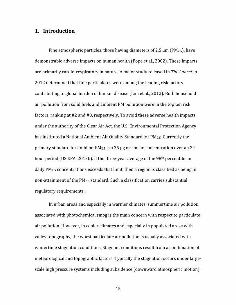
1. Introduction
Fine atmospheric particles, those having diameters of 2.5 µm (PM2.5), have
demonstrable adverse impacts on human health (Pope et al., 2002). These impacts
are primarily cardio-respiratory in nature. A major study released in The Lancet in
2012 determined that fine particulates were among the leading risk factors
contributing to global burden of human disease (Lim et al., 2012). Both household
air pollution from solid fuels and ambient PM pollution were in the top ten risk
factors, ranking at #2 and #8, respectively. To avoid these adverse health impacts,
under the authority of the Clear Air Act, the U.S. Environmental Protection Agency
has instituted a National Ambient Air Quality Standard for PM2.5. Currently the
primary standard for ambient PM2.5 is a 35 µg m-3 mean concentration over an 24-
hour period (US EPA, 2013b). If the three-year average of the 98th percentile for
daily PM2.5 concentrations exceeds that limit, then a region is classified as being in
non-attainment of the PM2.5 standard. Such a classification carries substantial
regulatory requirements.
In urban areas and especially in warmer climates, summertime air pollution
associated with photochemical smog is the main concern with respect to particulate
air pollution. However, in cooler climates and especially in populated areas with
valley topography, the worst particulate air pollution is usually associated with
wintertime stagnation conditions. Stagnant conditions result from a combination of
meteorological and topographic factors. Typically the stagnation occurs under large-
scale high pressure systems including subsidence (downward atmospheric motion),
16
clear skies, and low surface wind speeds. During the wintertime in the absence of
strong solar heating of the surface, the planetary boundary layer (PBL) is shallow
with minimal vertical mixing. At night under clear skies, a strong surface
temperature inversion can occur and, with snow-covered surfaces, this can extend
through the daylight hours. Dilution of pollutants is dampened and high pollutant
concentrations are often observed. This phenomenon is exacerbated by valley
topography where cold air pooling can occur. Thus stagnant conditions within
valleys can lead to exceptionally high pollution levels. Such wintertime valley
stagnation events have been studied previously in Idaho’s Treasure Valley (Kuhns et
al., 2003; Stockwell et al., 2003), in the Cache Valley in Utah (Silva et al., 2007), and
in the Chamonix Valley in France (Chazette et al., 2005).
Currently, the Yakima region in Washington is in attainment for PM2.5.
However there had been an upward trend in PM2.5 in recent years, primarily during
winter, and for a time a nonattainment classification was considered a possibility.
Values have since dropped, but nonetheless the Washington Department of Ecology
desired a more complete understanding of the conditions that led to elevated PM2.5
levels in the Yakima region. To achieve this goal, they contracted with researchers at
Washington State University in Pullman (WSU) and at Central Washington
University in Ellensburg (CWU) to complete the Yakima Air Wintertime Nitrate
Study (YAWNS). The major focus of YAWNS was an intensive observation period in
the Yakima region during January 2013. The resulting data were analyzed during
the rest of 2013. This report describes the data and the resulting analysis.
17
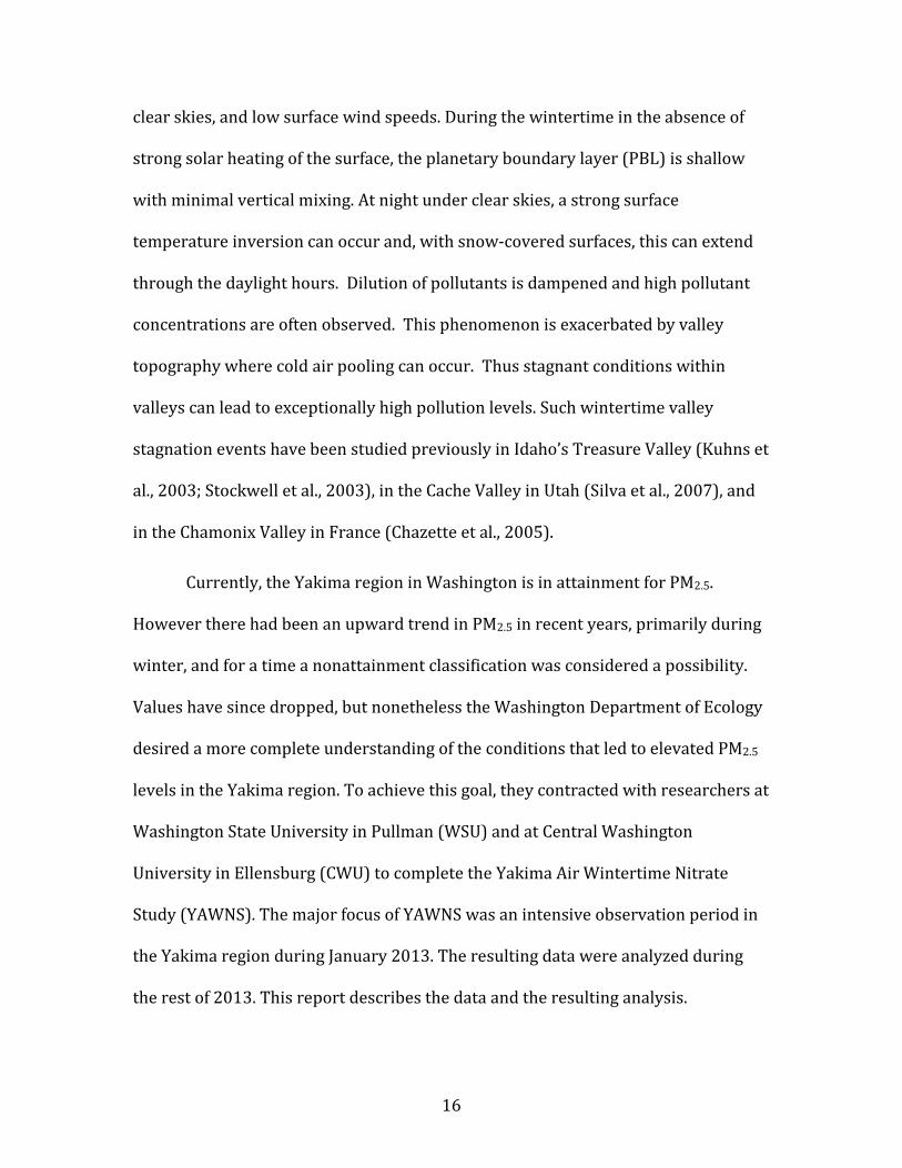
Figure 1.1. Contribution of ammonium nitrate (NH4NO3) to total PM2.5 in Washington. Map is based
on measured aerosol speciation data collected through 2009, spatially interpolated with CMAQ-modeled data at a 12km resolution. Map created and provided by Dr. Ranil Dhammapala, Washington Department of Ecology.
Yakima is unusual within Washington in that a significant fraction of the
PM2.5 during winter is comprised of particulate nitrate, usually in the chemical form
of ammonium nitrate (NH4NO3). Particulate nitrate makes up a larger fraction of
PM2.5 in Yakima and south central Washington than it does anywhere else in the
state (Figure 1.1). Nitrate levels are especially important during episodes of high
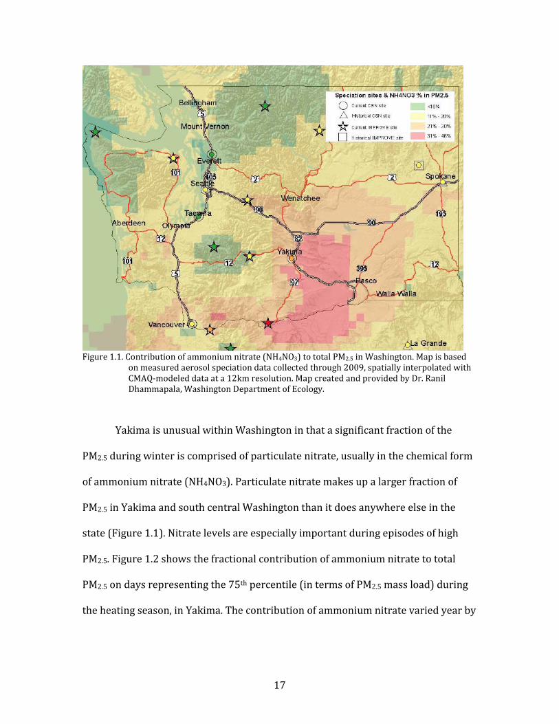
PM2.5. Figure 1.2 shows the fractional contribution of ammonium nitrate to total
PM2.5 on days representing the 75th percentile (in terms of PM2.5 mass load) during
the heating season, in Yakima. The contribution of ammonium nitrate varied year by
18
year, but was always 15-25% of the total PM2.5 on these days with elevated
particulate pollution.
Figure 1.2. Fractional contribution of major chemical constituents to PM2.5 on elevated particulate
pollution days during the heating season in Yakima. The data shown represent the 75th percentile in PM2.5 concentration for each year’s heating season when speciation data are available. Numbers on each bar indicate the PM2.5 mass measured at the 75th percentile for each year. (NH4)2SO4 is ammonium sulfate; NH4NO3 is ammonium nitrate, EC is elemental carbon (i.e., soot); and OMC is organic matter carbon. Figure created and provided by Dr. Ranil Dhammapala, Washington Department of Ecology.
1.1. Control of Wood Smoke Emissions
The dominant component of wintertime PM2.5 in Yakima is organic matter.
At present, the primary strategy employed in Washington to reduce PM2.5 during
wintertime is to control the emissions from biomass burning, including burning
wood for home heating and outdoor burning of yard debris and orchard tearouts.
This is the case in the Yakima region as well. The Yakima Regional Clean Air Agency
(YRCAA) has a successful wood stove exchange that provides financial incentives to
encourage residents to exchange older, dirtier, less efficient wood stoves for less

19
polluting certified models. In addition, during periods when PM2.5 levels are
expected to reach unhealthy level, air quality managers can implement burn bans.
These bans can be either a Stage 1 or Stage 2 level.
During a Stage 1 burn ban:
1) No burning is allowed in fireplaces and uncertified wood stoves,
unless it is your only adequate source of heat. This includes the use of
manufactured logs such as Duraflame or Javalogs.
2) Pellet stoves, EPA-certified wood stoves and natural gas or propane
fireplaces may be used.
3) No visible smoke is allowed from any solid fuel burning devices,
beyond a 20 minute start-up period.
During a Stage 2 burn ban:
1) No burning is allowed in any fireplace, pellet stove or wood stove
(certified or not), unless it is your only adequate source of heat.
2) Natural gas or propane stoves and fireplaces may be used.
3) No visible smoke is allowed from any solid fuel-burning device at any
time.
All outdoor burning is prohibited during a burn ban, even in areas where otherwise
permitted by law (RCW 70.94.473).
While burn bans have proven effective as a means of reducing particulate
pollution levels and avoiding adverse health effects on occasion (Washington
20
Department of Ecology, 2011), there remain implementation challenges and
questions as to their effectiveness.
1.2. Particulate Nitrate
The presence of elevated nitrate in PM2.5 during wintertime in the Yakima
region provides an additional target for control strategies, potentially
complementing the strategies in place to control PM2.5 from wood smoke. Evaluating
this possibility requires first obtaining an improved understanding of the sources
and chemical transformations that lead to the presence of elevated nitrate in the
region’s PM2.5. Gaining that understanding is the primary motivation for the YAWNS
project and for this report. An additional motivation is to provide a more general
characterization of the atmospheric environment of the Yakima region during
winter and describe how emissions, atmospheric chemistry, and meteorology
interact to drive the PM2.5 observed.
Particulate nitrate exists primarily as ammonium nitrate (NH4NO3), either as
a solid or dissolved as part of an aqueous solution. A good review of the atmospheric
chemistry leading to ammonium nitrate formation can be found in Seinfeld and
Pandis (2006). In the absence of water or other species, ammonium nitrate in the
particle phase exists in equilibrium with gas-phase nitric acid (HNO3) and ammonia
(NH3):
NH3(𝑔) + HNO3(𝑔) ↔ NH4NO3(𝑠) [R 1.1].
When only these species are present, then the equilibrium can be straightforwardly
described using an equilibrium constant Kp(T), which is equal to the product of the
21
gas-phase ammonia and nitric acid partial pressures. If the product of the gas-phase
HNO3 and NH3 concentrations is less than the value of the equilibrium constant then
no particulate nitrate will condense. Once the gas phase is saturated with ammonia
and nitric acid, any excess must condense into the particle phase to form ammonium
nitrate. At wintertime temperatures, the equilibrium is driven strongly toward the
condensed phase, meaning that relatively more ammonium nitrate will form in
winter than in summer for the same initial gas concentrations.
The introduction of water, sulfate, and organic species, all of which are
present in the ambient atmosphere, adds more complexity to the ammonium nitrate
formation mechanism. When sufficient water is present, a condensed aqueous phase
will form, and ammonium, nitrate, and sulfate will each exist primarily in their ionic
forms. Ammonia will condense preferentially with sulfate compounds (which
condense irreversibly), so in practical terms all sulfate must be fully neutralized
before any ammonia is available to react with nitric acid to form nitrate aerosol. The
aqueous phase also affects the equilibration of ammonium nitrate independently-
some fraction of the ammonia and nitric acid will condense even if the product of
their gas-phase partial pressures is below the value indicated by Kp(T). In these
cases, the equilibration calculation is complex enough to usually require a numerical
solution.
Ammonia in the atmosphere results mostly from primary agricultural
emissions, with smaller contributions from natural sources, biomass burning, and
human activities (Seinfeld and Pandis, 2006). In contrast, primary emissions of
nitric acid are relatively small. Nitric acid forms in the atmosphere as a result of the
22
oxidation of NO and NO2, the major nitrogen oxide species (NOx). NOx is released to
the atmosphere mostly as a byproduct of fossil fuel and other fuel combustion.
There are two major mechanisms for converting NOx to HNO3. During daytime,
HNO3 forms from the reaction of NO2 with photolytically-generated hydroxyl
radical:
OH + NO2 + M → HNO3 + M [R 1.2].
Here, OH is the hydroxyl radical and M is any third molecule (typically nitrogen or
oxygen) that absorbs energy during the reactive collision. At night, OH
concentrations are low due to the absence of sunlight but can be formed in other
reactions, such those between O3 and alkenes. In winter months daytime OH
concentrations would be low due to reduced ultra-violet photon flux compared to
summer. Thus nitric acid production rates from R1.2 would be low and may not be
significant in winter. At night, two other chemical reactions are possible to produce
particulate nitrate. Both reaction pathways involve the nitrate radical (NO3, distinct
from particulate nitrate). During the day, NO3 is rapidly photolyzed and thus does
not exist at significant concentrations during the day, even in winter. NO3 is rapidly
removed through reaction with NO, so NO3 chemistry only occurs when NO mixing
ratios are suitably low. NO3 radical is made at night when O3 reacts with NO2 and
can lead to PM nitrate production through N2O5 uptake and subsequent hydrolysis
on particles:
NO2 + O3 → NO3 + O2 [R 1.3];
NO2 + NO3 + M ↔ N2O5 + M [R 1.4];
23
N2O5 + H2O(𝑙) → 2HNO3 [R 1.5].
Another pathway is reaction of NO3 radical with aldehydes, such as
formaldehyde (HCHO) and acetaldehyde, associated with vehicle emissions:
NO3 + HCHO → HNO3 + HCO [R 1.6];
HCO + O2 → HO2 + CO [R 1.7];
HO2 + NO → HO + NO2 [R 1.8];
OH + NO2 + M → HNO3 + M [R 1.2].
Together the HNO3 production mechanisms are the major pathways for removal of
NOx from the atmosphere and the source for particulate nitrate.
24
2. Project Objectives and Tasks
The motivation for the YAWNS study was the need to determine the causes of
the particulate nitrate frequently observed at Yakima during winter. Meeting this
goal required obtaining field observation data that could be analyzed to improve
current understanding of the sources, meteorological conditions, and atmospheric
chemistry that leads to elevated particulate nitrate levels in the region. An
additional motivation was to provide a more general characterization of the
atmospheric environment in Yakima during winter for comparison with and
evaluation of the AIRPACT-4 regional air quality forecast model.
To achieve the project objectives, the YAWNS study was divided into the
following major tasks:
1) Instrument Calibration and MACL Integration at WSU;
2) Field Observations;
3) Data Reduction and Validation;
4) Data Analysis to Address Project Objectives; and
5) Reporting of Results.
Task 1: The equipment listed in Table 5.1 were extensively tested at WSU
and CWU and integrated into the MACL trailer for deployment to Yakima.
Arrangements were made to allow continuous sampling at the two project sites for a
three-week period in January 2013. Data logging capabilities and outputs of each
25
instrument were finalized at this time, including the required modifications to data
acquisition systems. Task 1 was completed on December 31, 2012.
Task 2: Continuous on-site air monitoring operations were conducted in
Yakima (5-27 January 2013) and Toppenish (11 December 2012 - 28 January 2013).
On-site activities were carried out by WSU and CWU staff with assistance from the
Washington Department of Ecology. On-site operations included: 1) inspection of
instruments and data from the acquisition systems; 2) periodic performance tests;
3) documentation of instrument, station, and meteorological conditions; 4)
preventive and corrective maintenance; and 6) transmission of data and
documentation. On-site operations were supported by additional Pullman-based
WSU staff; this support included: 1) periodic download and examination of field
data; 2) replenishment of consumables and supplies; 3) operations review with field
staff; 4) laboratory analysis of collected samples; and 5) site visits as needed for
instrument calibration, repair, and maintenance. Uploaded data were assembled
into a comprehensive database in preparation for post-study validation. Task 2 was
completed on January 28, 2013.
Task 3: Time series and scatterplots for all primary data products were
examined to identify outliers. Validation levels were assigned to aid users in
assessing the reliability of the data sets for analysis. All validated data was compiled
in an organized, secure online data repository available to both WSU and Ecology
staff. This was completed by August 30, 2013.
26
Task 4: Advanced data analysis was conducted to address Ecology’s and
WSU’s major project objectives. This included analyzing correlations among
measured chemical and meteorological parameters, assessing the contributions of
woodsmoke, describing the stagnation conditions during the study period, and
conducting a positive matrix factorization analysis on the PM composition data. This
work was completed in part by WSU researchers in Pullman, and in part by Graham
VanderSchelden, a WSU graduate student working directly with Ecology staff during
the summer of 2013. Data analysis activities within the project scope were
completed on February 1, 2014.
Task 5: WSU has prepared this final report summarizing the project
activities and data assessment. Summaries of major data analysis activities are
provided, but full reports of all post-experiment research are beyond this scope of
this report. We anticipate that WSU and Ecology staff will continue to collaborate to
produce manuscripts for the peer-reviewed literature as an outcome of the YAWNS,
but such efforts are beyond the specific requirements of this project. With the
exception of these final manuscripts, final reporting will be complete by February 28,
2014.
27
3. Report Format
This report is organized into nine major chapters, with references and
appendices also included. Chapter 1 of this report introduces the background
knowledge to place the YAWNS study in context with other work. Chapter 2
presents the objectives and tasks of the YAWNS project as detailed in our initial
work plan. This chapter describes the report format. Chapter 4 describes the study
conditions, including discussions of the two YAWNS measurement sites as well as
the overall meteorological conditions and the burn ban properties during the study
period. Chapter 5 discusses the instrumentation deployed from WSU and CWU, with
additional detail provided in the report appendices. Chapter 6 discusses our quality
assurance and quality control approach, and also provides basic time series results
for most parameters studied during YAWNS. Chapter 7 describes the positive matrix
factorization analysis used to derive source factors for the organic PM. Chapter 8
describes our detailed analysis of our collected data, designed to address our
primary and secondary motivating questions for the study. Chapter 9 summarizes
the reports major findings and outlines expected future research directions for the
research team.
28
4. Study Conditions
The YAWNS field study took place during a three-week period from 5-27
January 2013, based in Yakima, Washington. Yakima is a small city (population
93,101, estimated 2012) located within the Upper Yakima Valley. The valley is
bounded by the Cascade Mountains to the immediate west, and by lines of hills to
the north and south that eventually merge several miles to the east. The topography
forms an enclosed basin at the surface that restricts horizontal air flow within the
valley. The Upper Yakima Valley connects to the Lower Yakima Valley via Union Gap,
located a few miles south of central Yakima. The Upper Valley also connects to the
Wenas Valley to the north of Yakima.
Yakima has a semi-arid climate due largely to it location in the rain shadow
of the Cascade Mountains. January is its second wettest month (after December),
with 28.7 mm of precipitation falling on average (1981-2010 mean). Mean daily
high and low temperatures during January are 38.8 and 23.8 °F, respectively,
making it the second coldest month of the year on average (trailing December)
(NOAA NOWData, 2013).
4.1. Site Descriptions
To address the study objectives, a primary site was established in central
Yakima. The goal at this site was to measure a comprehensive suite of pollutant
concentrations and local meteorology at a location that would be representative of
the city’s air quality. Additional instrumentation was located at an existing air
29
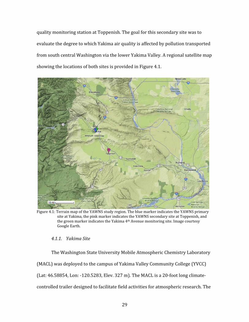
quality monitoring station at Toppenish. The goal for this secondary site was to
evaluate the degree to which Yakima air quality is affected by pollution transported
from south central Washington via the lower Yakima Valley. A regional satellite map
showing the locations of both sites is provided in Figure 4.1.
Figure 4.1: Terrain map of the YAWNS study region. The blue marker indicates the YAWNS primary
site at Yakima, the pink marker indicates the YAWNS secondary site at Toppenish, and the green marker indicates the Yakima 4th Avenue monitoring site. Image courtesy Google Earth.
4.1.1. Yakima Site
The Washington State University Mobile Atmospheric Chemistry Laboratory
(MACL) was deployed to the campus of Yakima Valley Community College (YVCC)
(Lat: 46.58854, Lon: -120.5283, Elev. 327 m). The MACL is a 20-foot long climate-
controlled trailer designed to facilitate field activities for atmospheric research. The
30
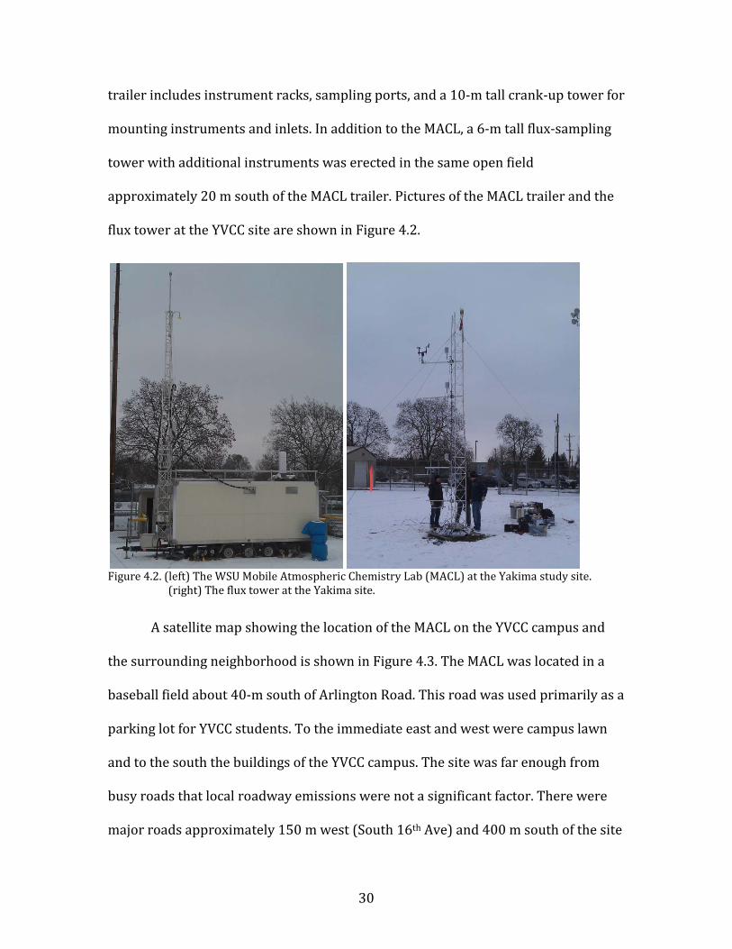
trailer includes instrument racks, sampling ports, and a 10-m tall crank-up tower for
mounting instruments and inlets. In addition to the MACL, a 6-m tall flux-sampling
tower with additional instruments was erected in the same open field
approximately 20 m south of the MACL trailer. Pictures of the MACL trailer and the
flux tower at the YVCC site are shown in Figure 4.2.
Figure 4.2. (left) The WSU Mobile Atmospheric Chemistry Lab (MACL) at the Yakima study site.
(right) The flux tower at the Yakima site.
A satellite map showing the location of the MACL on the YVCC campus and
the surrounding neighborhood is shown in Figure 4.3. The MACL was located in a
baseball field about 40-m south of Arlington Road. This road was used primarily as a
parking lot for YVCC students. To the immediate east and west were campus lawn
and to the south the buildings of the YVCC campus. The site was far enough from
busy roads that local roadway emissions were not a significant factor. There were
major roads approximately 150 m west (South 16th Ave) and 400 m south of the site
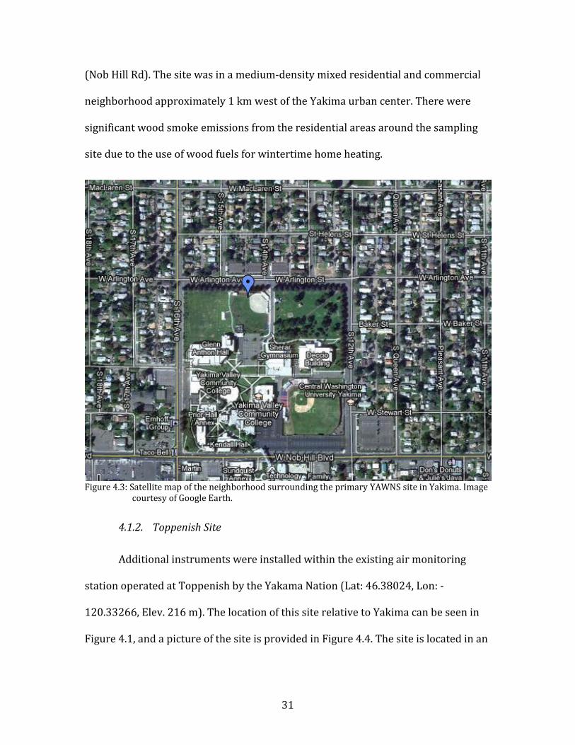
31
(Nob Hill Rd). The site was in a medium-density mixed residential and commercial
neighborhood approximately 1 km west of the Yakima urban center. There were
significant wood smoke emissions from the residential areas around the sampling
site due to the use of wood fuels for wintertime home heating.
Figure 4.3: Satellite map of the neighborhood surrounding the primary YAWNS site in Yakima. Image
courtesy of Google Earth.
4.1.2. Toppenish Site
Additional instruments were installed within the existing air monitoring
station operated at Toppenish by the Yakama Nation (Lat: 46.38024, Lon: -
120.33266, Elev. 216 m). The location of this site relative to Yakima can be seen in
Figure 4.1, and a picture of the site is provided in Figure 4.4. The site is located in an
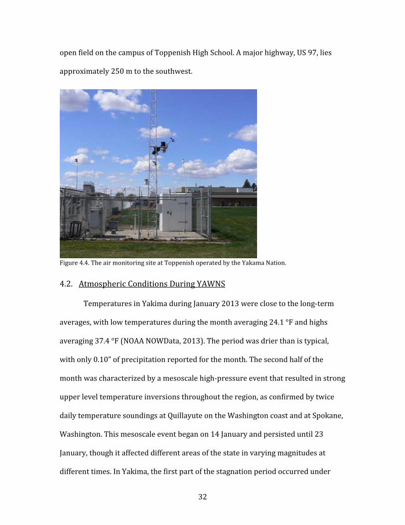
32
open field on the campus of Toppenish High School. A major highway, US 97, lies
approximately 250 m to the southwest.
Figure 4.4. The air monitoring site at Toppenish operated by the Yakama Nation.
4.2. Atmospheric Conditions During YAWNS
Temperatures in Yakima during January 2013 were close to the long-term
averages, with low temperatures during the month averaging 24.1 °F and highs
averaging 37.4 °F (NOAA NOWData, 2013). The period was drier than is typical,
with only 0.10” of precipitation reported for the month. The second half of the
month was characterized by a mesoscale high-pressure event that resulted in strong
upper level temperature inversions throughout the region, as confirmed by twice
daily temperature soundings at Quillayute on the Washington coast and at Spokane,
Washington. This mesoscale event began on 14 January and persisted until 23
January, though it affected different areas of the state in varying magnitudes at
different times. In Yakima, the first part of the stagnation period occurred under
33
clear sky conditions, and the nighttime surface temperature inversions led to
significant buildup of PM2.5. Beginning on 16 January the area became cloudy and
PM2.5 dropped significantly.
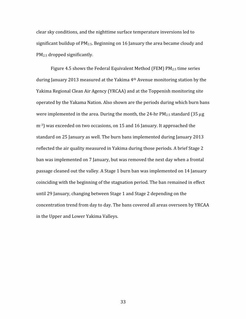
Figure 4.5 shows the Federal Equivalent Method (FEM) PM2.5 time series
during January 2013 measured at the Yakima 4th Avenue monitoring station by the
Yakima Regional Clean Air Agency (YRCAA) and at the Toppenish monitoring site
operated by the Yakama Nation. Also shown are the periods during which burn bans
were implemented in the area. During the month, the 24-hr PM2.5 standard (35 µg
m-3) was exceeded on two occasions, on 15 and 16 January. It approached the
standard on 25 January as well. The burn bans implemented during January 2013
reflected the air quality measured in Yakima during those periods. A brief Stage 2
ban was implemented on 7 January, but was removed the next day when a frontal
passage cleaned out the valley. A Stage 1 burn ban was implemented on 14 January
coinciding with the beginning of the stagnation period. The ban remained in effect
until 29 January, changing between Stage 1 and Stage 2 depending on the
concentration trend from day to day. The bans covered all areas overseen by YRCAA
in the Upper and Lower Yakima Valleys.
34
Figure 4.5. Hourly time series PM2.5 levels measured at the Yakima 4th Avenue and Toppenish
monitoring sites during January 2013. Shaded areas indicate Stage 1 and Stage 2 burn bans, as labeled.
35
5. Instrumentation
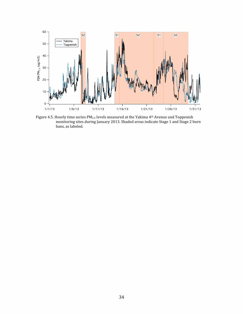
The instruments deployed to Yakima and Toppenish during YAWNS are
listed in Table 5.1 below. The table includes a brief description of the measurement,
details on the instrument used, and the sampling period for the instrument.
Table 5.1. Summary of YAWNS measurements.
Primary Site in Yakima
Measurement Instrument Sampling Period
NOx & NOy Air Quality Designs dual-channel instrument (NO, NO2, and NOy) 1 min
NH3 Custom ammonia sampler w/
laboratory analysis 8 / 16 hrs
CO AeroLaser Vacuum UV instrument 1 min O3 Dasibi ozone monitor 1 min
Trace organic gases(1)
Proton Transfer Reaction – Mass Spectrometer (PTR-MS) 1 min
Aerosol number concentration Condesation Particle Counter (CPC) 1 min
Aerosol composition
High Resolution Aerosol Mass Spectrometer (HR-AMS) 2 min
Aerosol black carbon content
Single Particle Soot Photometer (SP2) 1 min
Particle size distribution
(0.020-0.700 mm)
Scanning Mobility Particle Sizer (SMPS) 5 min
PBL Height Vaisala Ceilometer 30 min Meteorological
data Vaisala WXT package 1 min
Satellite Site in Toppenish
Measurement Instrument Sampling Period
NOx TECO 42 NOx monitor 1 min CO TECO 48 CO monitor 1 min
(1) See Table 5.2 for the list of trace organic species measured.
36
5.1. Particle Instrumentation
5.1.1. Aerosol Inlet
Aerosols were sampled from approximately 7 m above ground level via an
inlet mounted to the MACL crank-up tower. Air was pulled through this inlet at a
total flow rate of approximately 4 liters per minute (lpm). The inlet line outside was
a 0.5” outer diameter copper tube. This tube was hooked downward at the inlet to
prevent precipitation from entering the inlet. The inlet line was also wrapped in
heating tape and was thermostated to approximately 50 ˚F; this was done to prevent
ice buildup within and around the inlet. Once inside the MACL trailer, the whole
aerosol was passed through a Nafion dehumidifier (PermaPure Model MD-110-24S-
4). This was done to dry the particles prior to sampling for easier intercomparions
of the different aerosol measurements.
5.1.2. Condensation Particle Counter (CPC)
The total particle number concentration (Ntot) was monitored using an
Ultrafine CPC (Model 3776, TSI Inc., Shoreview, MN). The CPC operates by
condensing butanol vapor onto particles such that they grow large enough to be
detectable on a single particle basis by laser light scattering. The Model 3776 CPC
used during YAWNS has a nominal size cutoff of 2.5 nm. Raw data from the CPC
were stored at one-second time intervals via custom control software developed in
LabView.
37
5.1.3. Scanning Mobility Particle Sizer (SMPS)
The particle number size distribution was measured using a custom-built
SMPS assembled at WSU. Major components for the SMPS were purchased TSI, Inc.
(Shoreview, MN). These included a differential mobility analyzer (DMA; TSI Model
308100) and a CPC (TSI Model 3775). Instrument control was via custom software
developed using LabView (National Instruments, Austin, TX). Details on the
operation and calibration of the SMPS system during YAWNS are provided in
Appendix 11.1. The settings chosen for the study allowed the particle size
distribution from 20-800 nm to be measured approximately every five minutes.
In addition to its use for ambient measurements during YAWNS, the SMPS
also served as the primary calibration tool for the high-resolution aerosol mass
spectrometer (HR-AMS) and the single particle soot photometer (SP2). For these
calibrations, a nebulizer system was used to generate a fine mist from a solution or
mixture of known composition. The water was next removed using a diffusion dryer,
leaving a population of dry calibration particles of known composition. These
particles were then size-selected with the DMA component of the SMPS and then
split between the CPC component of the SMPS and the instrument to be calibrated.
In this way the instrument being calibrated was provided a aerosol sample of
known size, composition, and concentration. During these calibration periods, it was
not possible to also measure the ambient particle size distribution.
38
5.1.4. High-Resolution Aerosol Mass Spectrometer (HR-AMS)
The composition of non-refractory submicron particulate material was
measured using an Aerodyne high-resolution time-of-flight aerosol mass
spectrometer (HR-AMS). The HR-AMS allows for the direct separation and
measurement of most ions at the same nominal m/z, quantification of organic
particulate mass and several inorganic species, and the determination of the size
distribution of all ions. The AMS uses automated data analysis routines to classify
the peaks in the mass spectrum into a finite number of classes of compounds,
including organics, ammonium, sulfate, nitrate, and chloride. The instrument
operates in two modes for ion transmission, referred to as V-mode and W-mode. V-
mode is a single-reflection configuration allowing for higher sensitivity at somewhat
lower resolution, while W-mode is a two-reflection configuration offering a lower
sensitivity but higher resolution. In both modes, aerosol particles enter through a
sampling inlet at a flow rate of approximately 1.5 cm3 s-1 and are transmitted
through an aerodynamic lens that first focuses particles into a narrow beam using
six apertures of sequentially decreasing size. This focusing greatly concentrates the
particles relative to the surrounding air.
The focused aerosol beam is finally accelerated in a supersonic expansion,
caused be the difference in pressure between the sampling and sizing chambers.
This acceleration also gives different velocities to aerosols of different sizes. After
passing through the lens, the aerosols next pass through a mechanical chopper that
can open or close to enter the particle-sizing chamber. At this point the instrument
is typically alternated between two modes of operation- mass spectrum (MS) mode
39
and particle time-of-flight (PTOF) mode. Only MS-mode data are included in this
report. In MS mode, particles travel unimpeded through the particle-sizing chamber
until they impact onto a resistively-heated porous tungsten surface held at 600 °C
where the volatile and semi-volatile portions of the aerosols are vaporized and
immediately ionized using 70-eV electron impact ionization. The mass spectrometer
detects the positive ion fragments generated by the electron impact ionization and
determines the mass-to-charge (m/z) distribution of the particle beam. The HR-AMS
detects non-refractory species that can evaporate rapidly at the vaporizer
conditions (mostly volatile and semi-volatile components). These include sulfate,
nitrate, ammonium, chloride, and total organic matter. Other non-volatile
constituents, such as crustal oxides, sea salt, and black carbon, are not detectable. A
more detailed description of the measurement approach for the HR-AMS and its
operation and calibration during YAWNS is provided in Appendix 11.2.
5.1.5. Single-Particle Soot Photometer (SP2)
The black carbon (BC) mass in individual particles between ~80-650 nm was
determined using a Single Particle Soot Photometer (SP2) (Schwarz et al., 2006).
The SP2 was adjusted following the recommendations detailed in Laborde et al.
(2012), and the incandescence signal was calibrated using fullerene soot particles
(Alpha Aesar; #L20W054) that were size selected using a differential mobility
analyser. Data analysis was conducted using the Paul Scherrer Institut Toolkit.
40
5.2. Trace Gas Instrumentation
5.2.1. Gas Phase Instrumentation Inlet
Air sample for the gas phase instrumentation was supplied by a common
sample line. This sample line consisted of 0.5” outer diameter PFA tubing that was
attached to the crank up meteorological tower with the inlet at a height of
approximately 10 m, as seen in Figure 4.2. A funnel around the inlet protected the
line from ingestion of snow and rain. The tube ran into the trailer and was attached
to a diagram pump that pulled air through the tube at approximately 30 liters per
minute. The gas phase instruments (PTR-MS, O3, CO, CO2) sub-sampled from this
flow. Instruments were protected from particle contamination by in-line Teflon
membrane filters. The NOx/NOy analyzer had its own inlet system enclosed in a
NEMA enclosure mounted to the metrological tower approximately 1 m below the
aerosol inlet. The NOx/NOy inlet system contained a heated molybdenum oxide
catalyst for NOy conversion and a photolysis cell for NO2 conversion. The sample
inlet consisted of a short piece of heated 0.25” outer diameter PFA tubing that
protruded approximately 1 inch from beneath the enclosure. The PFA tubing below
and within the enclosure was resistively heated and termostated to 30 °C to prevent
loss of nitric acid.
5.2.2. NOx/NOy Analyzer
NO, NO2, and NOy were measured using a two-channel chemiluminescence
NO detector (Air Quality Design). NOy was measured continuously on one channel
by conversion to NO with a molybdenum oxide catalytic converter. The other
41
channel measured NO for 30 seconds then NOx (NO + NO2) for 30 seconds in an
alternating cycle. NO2 was photolyzed to NO via a blue light converter. The
difference between the measured NOx and NO was reported as NO2. NOy is defined
as NOx plus the compounds that result from the oxidation of NOx. This includes but
is not limited to: NO3, N2O5, HNO3, HONO, PAN, organic nitrates, and particulate
nitrate. The instrument response time to NO for both channels is less than 1 second.
Data were recorded at 1 Hz and reported at 1-minute intervals. Instrument
sensitivity was determined using an NO calibration gas of 500 ppmv ± 1%, NIST
traceable, (Scott-Marrin, Inc.) diluted in dry zero air to provide a 250 ppbV NO
calibration level. Calibration of the NO2 converter efficiency was performed using
gas phase titration of NO to NO2. A detailed description of the measurement
approach for the NOx/NOy analyzer and it operation and calibration during YAWNS
is provided in Appendix 11.3.
5.2.3. Aerolaser Vacuum UV Carbon Monoxide Analyzer
Carbon monoxide (CO) was measured using a vacuum UV florescence
instrument (Aerolaser GmbH, Germany). The instrument allows fast response and
sensitive measurements of CO; the response time is approximately 1 second and the
detection limits is approximately 50 pptv. The instrument was calibrated by
standard addition whereby a low flow of a 101.6 ppmv ± 1% NIST traceable
standard (Scott Marrin) was added to the sample air every 4 hours for
approximately 1 minute to keep track of potential sensitivity drifts. Background
response to zero air was determined by passing ambient air through a CO
42
destruction catalyst. Data were collected a 1 Hz and reported as 1 minute averages.
A detailed description of the calibration and data reduction procedures for the CO
measurement can be found in Appendix 11.4.
5.2.4. Proton Transfer Reaction Mass Spectrometer (PTR-MS)
VOC measurements were made using a PTR-MS instrument (Ionicon Analytik,
GmbH, Austria). The PTR-MS continuously measures organics in air by chemical
ionization using H3O+ as a proton transfer reagent ion. The method has been well
described in literature (Lindinger et al., 1998). Organic compounds with proton
affinities greater than that of water undergo fast proton transfer reactions with
H3O+:
R + H3O+ RH+ + H2O [R 5.1],
where R is the organic compound and RH+ is the product ion (M+1 ion). The ions
were detected with a quadrupole mass spectrometer. Compounds of interest in
urban atmospheres that can be measured with this approach include aromatic
compounds such as benzene and toluene, simple alcohols (methanol and ethanol)
and aldehydes (formaldehyde, acetaldehyde). The instrument is insensitive to
small alkanes, acetylene, and ethylene. For monoaromatic compounds that have
geometric isomers, such as the xylene isomers and ethylbenzene, the sum total of
these compounds is reported.
The proton transfer reaction occurs in an ion drift tube that enhances the
kinetic energy of the ions so that collisions with the bath gas (air) cause desolvation
of hydrated ions. For many compounds, R5.1 is dissociative at the kinetic energies
43
required for efficient desolvation, resulting in the formation of fragment ions that
complicate the interpretation of the PTR-MS mass spectrum as a simple M+1 mass
spectrum. To mitigate this problem the PTR-MS was operated at a lower drift tube
electric field, which requires sample drying. For the YAWNS field campaign, the
sampled air was dehumidified to -30 °C using a cold trap, allowing for the operation
of the PTR-MS drift tube at 80 Td (Jobson and McCoskey, 2010). Operation at 80 Td
(drift pressure 2.08 mbar, drift temperature 65 °C, drift voltage 327 V) allowed for
measurement of formaldehyde and significantly reduced fragmentation, improving
accuracy in the measurement of aromatic compounds. The PTR-MS was calibrated
by diluting a multi-component gas standard containing 13 compounds at 2 ppmv ±
5% (Scott Marrin) with humidified zero air to 19.8 ppbv. Formaldehyde sensitivity
was calibrated using a permeation tube (KinTek). A more detailed discussion of the
PTR-MS operation and calibration during YAWNS is presented in Appendix 11.5.
The PTR-MS performed full mass scans (m/z 31-150) 5-8 January. After 8
January, a suite of 45 organic ions was measured and data for 10 of these ions are
reported. For these 10 ions, we have confidence in their compound attribution and
PTR-MS sensitivity factors, and these data were well above compound detection
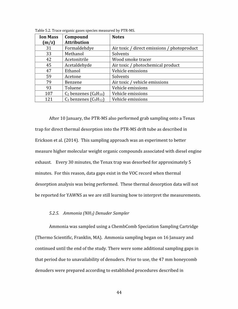
limits. These compounds are listed in Table 5.2. The mass spectrometer measures
each mass for a specified dwell time (1-5 seconds), and cycled through the list of 45
ions every minute. Data are thus reported every minute but should not be
construed as 1-minute averages.
44
Table 5.2. Trace organic gases species measured by PTR-MS.
Ion Mass (m/z)
Compound Attribution
Notes
31 Formaldehdye Air toxic / direct emissions / photoproduct 33 Methanol Solvents 42 Acetonitrile Wood smoke tracer 45 Acetaldehyde Air toxic / photochemical product 47 Ethanol Vehicle emissions 59 Acetone Solvents 79 Benzene Air toxic / vehicle emissions 93 Toluene Vehicle emissions
107 C2 benzenes (C8H10) Vehicle emissions 121 C3 benzenes (C9H12) Vehicle emissions
After 10 January, the PTR-MS also performed grab sampling onto a Tenax
trap for direct thermal desorption into the PTR-MS drift tube as described in
Erickson et al. (2014). This sampling approach was an experiment to better
measure higher molecular weight organic compounds associated with diesel engine
exhaust. Every 30 minutes, the Tenax trap was desorbed for approximately 5
minutes. For this reason, data gaps exist in the VOC record when thermal
desorption analysis was being performed. These thermal desorption data will not
be reported for YAWNS as we are still learning how to interpret the measurements.
5.2.5. Ammonia (NH3) Denuder Sampler
Ammonia was sampled using a ChembComb Speciation Sampling Cartridge
(Thermo Scientific, Franklin, MA). Ammonia sampling began on 16 January and
continued until the end of the study. There were some additional sampling gaps in
that period due to unavailability of denuders. Prior to use, the 47 mm honeycomb
denuders were prepared according to established procedures described in
45
Appendix 11.6. Briefly, the denuders were coated with 10 mL of a solution that
contained 1% phosphoric acid and 10% methanol. Denuders were prepared in
Pullman and then transported overnight to Yakima for use. Just prior to sampling,
the denuders were placed in the cartridge samplers that were mounted on a fence
approximately 10 m from the MACL trailer. Samples were collected by drawing air
through the cartridge at a flow rate of 10 L per min. Typically two samples were
collected per day– one 8-hr sample beginning at 09:00 and one 16-hr sample
beginning at 17:00. After sampling, denuders were removed from the sampling
cartridges and returned to Pullman for analysis. Analysis procedures are described
in Appendix 11.7. Briefly, ammonia was eluted from the denuders with 10 mL of
deionized water. Ammonia concentrations were then determined
spectrophotometrically with the Nitrogen-Ammonia Reagent Set, TNT,
AmVer™(Salicylate), Low Range kit (Hach Company, Loveland, CO) according to
manufacturer’s instructions. These solution concentrations the total mass collected
per sample, which was then converted to a mean atmospheric concentration during
the sample period. These concentrations were corrected to remove the small
artifacts found on blank denuders analyzed as a control.
5.2.6. CO2 and H2O Analyzer
Carbon dioxide and water vapor were measured by a LiCor 840A analyzer.
Factory response factors were used for the determination of CO2 and water vapor
mixing ratios. Instrument performance for CO2 was verified by measuring a
46
calibration tank containing 390 ppmv CO2 ±1 % (Scott Marrin). Data were recorded
at 1 Hz and one-minute averages were reported.
5.2.7. Ozone Monitor
Ozone was measured by UV absorption using a Daisibi 1008 monitor. This
instrument was calibrated against a dedicated secondary O3 standard instrument
owned by WSU. One-minute averages were reported.
5.3. Meteorological Instruments
5.3.1. Ceilometer
Atmospheric planetary boundary layer (PBL) heights and cloud base heights
were detected using a ceilometer (model CL31, Vaisala). This instrument measures
the optical backscatter intensity of light emitted in the near-infrared (wavelength =
910 nm). During YAWNS, the ceilometer was set to report vertical profiles from zero
to 4,500 m above ground level every 16 s, with a vertical resolution of 10 m.
Structures present in the backscatter retrieval (up to three cloud base heights and
three PBL heights) were identified using the Vaisala PBL height algorithm (version
3.5), which is the default setting in Vaisala BL-VIEW software and is based on the
gradient method (Vaisala, Inc., 2010). This method selects the maximum of the
negative gradient of the backscatter coefficient to be the top of the PBL. Individual
measurements were averaged over a 30-minute period for our analysis.
47
5.3.2. Weather Station
Two weather stations were deployed to the YAWNS site at Yakima. One, a
model WXT510 (Vaisala, Inc.) was mounted at 10 m atop the MACL’s crank-up
tower. The other, a model WXT520 (Vaisala Inc), was mounted about 6 m above the
ground on the flux-sampling tower. Both stations measured wind speed, wind
direction, air temperature, relative humidity, and atmospheric pressure. Unless
otherwise indicated, the weather data discussed in this report are from the WXT510
mounted on the MACL tower.
5.3.3. Flux Tower Measurements
Surface energy fluxes were measured using two eddy covariance systems
installed at 2.12 and 4.17 m above ground level on a 6-m tall aluminum flux-
sampling tower. Data from the flux tower were available beginning at 16:00 on 14
January and ending at 17:00 on 26 January. Each eddy covariance system consisted
of a three-dimensional sonic anemometer (CSAT3, Campbell Scientific, Inc.) and an
open-path carbon dioxide/water vapor (CO2/H2O) infrared gas analyzer (IRGA;
model LI 7500a, LI-COR, Inc.). Sensor signals from the eddy covariance systems
were recorded at 10 Hz using a datalogger (model CR5000, Campbell Scientific, Inc.).
The 10 Hz raw time-series data collected in this study were processed and corrected
to obtain eddy covariance fluxes by using a post-field data processing program.
Briefly, the virtual air temperature was converted to air temperature following the
procedure suggested by Campbell Scientific Inc.’s instruction manual (2006). The
raw 10 Hz time series data were checked for noise using the criterion that data with
48
automatic gain control (AGC) values (output from the LICOR 7500 sensor) greater
than 65 were removed. Data points were labeled as spikes when their magnitudes
exceeded 4.5 times the standard deviation in a running 600-point window. If the
number of continuous points meeting the spike criterion was less than four, then
these values would be replaced through linear interpolation; longer duration events
were not labeled as spikes. The planar fit method was used for coordinate system
transformation. Fluxes were then computed using a block average method. Sensible
and latent heat fluxes were obtained via 30-min mean covariance between vertical
velocity and the respective air temperature and water vapor density fluctuations.
Due to air density effects, latent heat flux was corrected according to the Webb
Pearman and Leuning (WPL) corrections (Webb et al., 1980).
Besides the eddy covariance measurements, a variety of micrometeorological
variables were measured as 30-minute averages of 1 s readings, including net
radiation (model CNR1, Kipp & Zonen Inc.), temperature and relative humidity
(model HMP45C, Vaisala Inc.), wind speed and direction (mode 03002, R.M. Young
Inc.), and soil temperature (model 109SS-L, Campbell Scientific, Inc.).
5.4. Toppenish Measurements
Carbon monoxide and NO and NOx were measured at the Toppenish site
using a TECO 48 monitor for CO and a TECO 42 monitor for NO and NOx.
Instruments were calibrated using the same standard gases used for the Yakima site
instruments before installation. Data was logged to a dedicated laptop as well as to
the Washington Department of Ecology telemetry system. The CO instrument had an
automatic zero cycle whereby ambient air was pulled through a destruction catalyst
49
(Sofnocat 514, Molecular Products). Air was sampled through a ¼” PFA Teflon
sample line with the inlet approximately 12 feet above the ground.
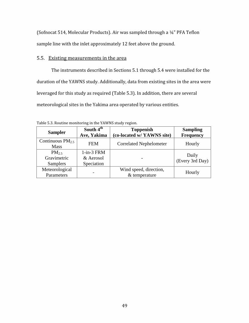
5.5. Existing measurements in the area
The instruments described in Sections 5.1 through 5.4 were installed for the
duration of the YAWNS study. Additionally, data from existing sites in the area were
leveraged for this study as required (Table 5.3). In addition, there are several
meteorological sites in the Yakima area operated by various entities.
Table 5.3. Routine monitoring in the YAWNS study region.
Sampler South 4th Ave, Yakima
Toppenish (co-located w/ YAWNS site)
Sampling Frequency
Continuous PM2.5 Mass FEM Correlated Nephelometer Hourly
PM2.5 Gravimetric
Samplers
1-in-3 FRM & Aerosol Speciation
- Daily (Every 3rd Day)
Meteorological Parameters - Wind speed, direction,
& temperature Hourly
50
6. Data
6.1. Data Quality
Each instrument described in Section 5 was evaluated separately for data
quality assurance. After processing, the data were carefully scrutinized and
compared against the instrument logs to ensure that data collected when
instruments did not meet operational specifications were removed from the final
results. Next, for ease of comparison, all data were average to a uniform 30-minute
time series. These time series begin at 00:00 on 5 January and end at 12:00 on 27
January 2013. The time-averaged data have been provided directly to Washington
Department of Ecology via a shared directory on a internet cloud storage site. Data
in these series are provided as the 30-minute data average for each time step, the
standard deviation, and a data flag. The standard deviation in the time series is
primarily a reflection of the time variability of the measured parameter over an
individual 30-minute period. Toppenish data are available for a longer time period,
from 12:00 on 11 December 2012 to 10:00 on 28 January 2013.
Data in the averaged time series were flagged to indicate the data
completeness within each 30-minute period. Periods with 5% data completion or
less were flagged “Little or No Data”; periods with 5-50% data completeness were
flagged as “Majority Missing Data”; periods with 50-95% completeness were flagged
as “Some Missing Data”; and data with more the 95% is flagged as “Complete Data”.
The completeness summary for all major parameters is presented in Table 6.1
below. There are two special cases for reporting data completion. For the ceilometer,
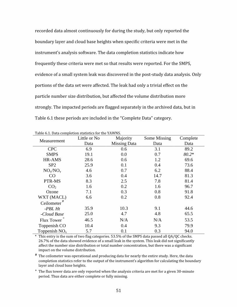
51
recorded data almost continuously for during the study, but only reported the
boundary layer and cloud base heights when specific criteria were met in the
instrument’s analysis software. The data completion statistics indicate how
frequently these criteria were met so that results were reported. For the SMPS,
evidence of a small system leak was discovered in the post-study data analysis. Only
portions of the data set were affected. The leak had only a trivial effect on the
particle number size distribution, but affected the volume distribution more
strongly. The impacted periods are flagged separately in the archived data, but in
Table 6.1 these periods are included in the “Complete Data” category.
Table 6.1. Data completion statistics for the YAWNS.
Measurement Little or No Data
Majority Missing Data
Some Missing Data
Complete Data
CPC 6.9 0.6 3.1 89.2 SMPS 19.1 0.0 0.7 80.2*
HR-AMS 28.6 0.6 1.2 69.6 SP2 25.9 0.1 0.4 73.6
NOx/NOy 4.6 0.7 6.2 88.4 CO 3.6 0.4 14.7 81.3
PTR-MS 8.3 2.5 7.8 81.4 CO2 1.6 0.2 1.6 96.7
Ozone 7.1 0.3 0.8 91.8 WXT (MACL) 6.6 0.2 0.8 92.4
Ceilometer #
-PBL Ht -Cloud Base
35.9 25.0
10.3 4.7
9.1 4.8
44.6 65.5
Flux Tower + 46.5 N/A N/A 53.5 Toppenish CO 10.4 0.4 9.3 79.9 Toppenish NOx 5.7 0.1 0.3 94.0
* This entry is the sum of two flag categories. 53.5% of the SMPS data passed all QA/QC checks. 26.7% of the data showed evidence of a small leak in the system. This leak did not significantly affect the number size distribution or total number concentration, but there was a significant impact on the volume distribution.
# The ceilometer was operational and producing data for nearly the entire study. Here, the data completion statistics refer to the output of the instrument’s algorithm for calculating the boundary layer and cloud base heights.
+ The flux tower data are only reported when the analysis criteria are met for a given 30-minute period. Thus data are either complete or fully missing.
52
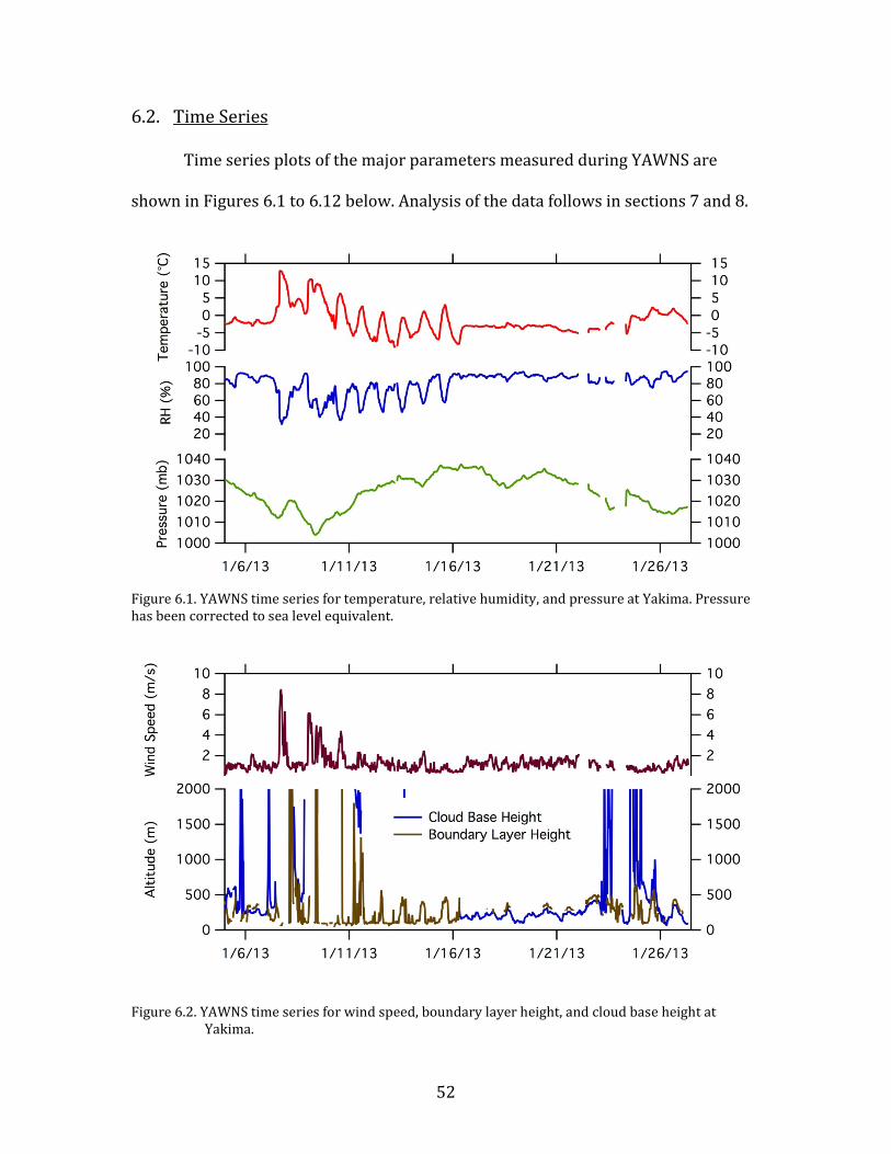
6.2. Time Series
Time series plots of the major parameters measured during YAWNS are
shown in Figures 6.1 to 6.12 below. Analysis of the data follows in sections 7 and 8.
Figure 6.1. YAWNS time series for temperature, relative humidity, and pressure at Yakima. Pressure has been corrected to sea level equivalent.
Figure 6.2. YAWNS time series for wind speed, boundary layer height, and cloud base height at Yakima.
53
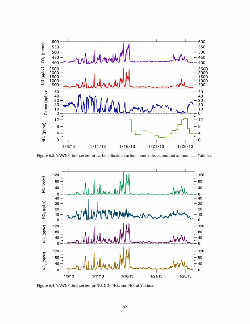
Figure 6.3. YAWNS time series for carbon dioxide, carbon monoxide, ozone, and ammonia at Yakima.
Figure 6.4. YAWNS time series for NO, NO2, NOx, and NOy at Yakima.
54
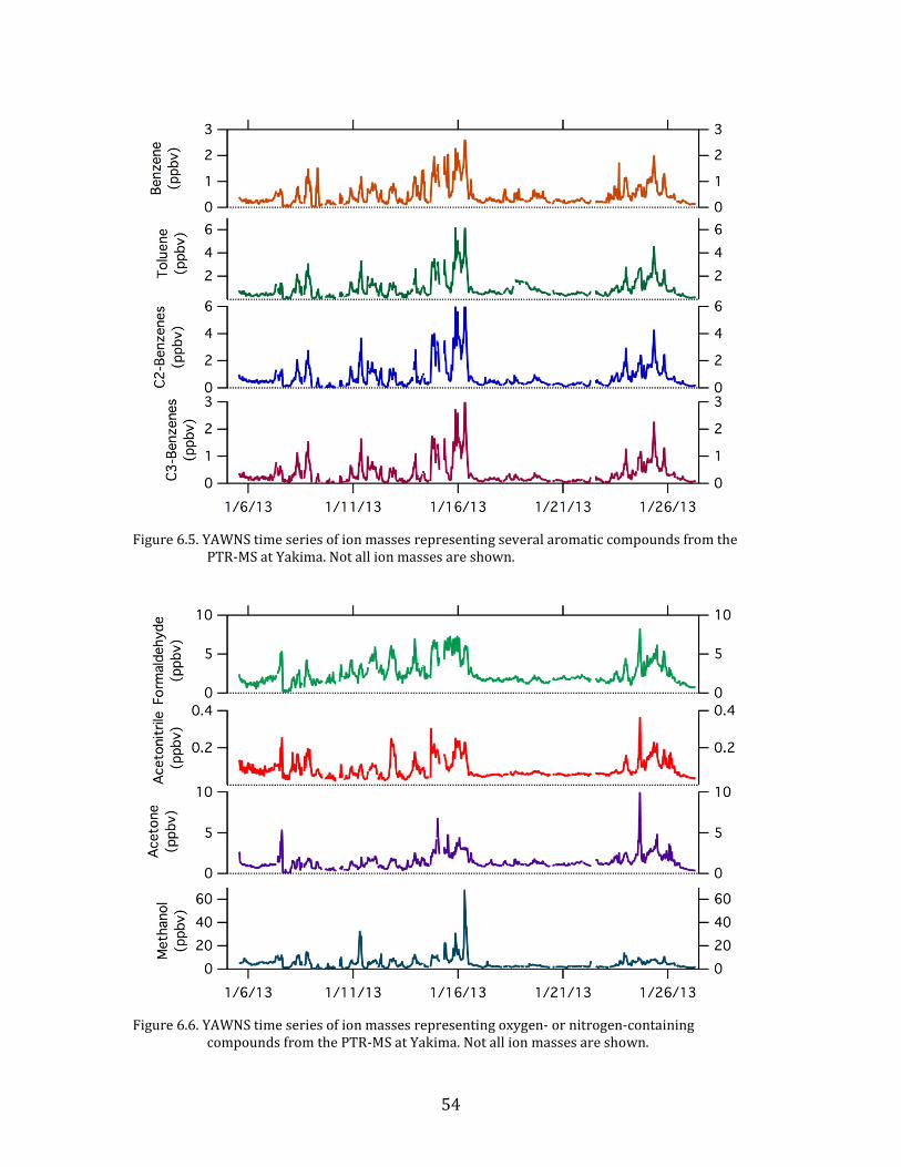
Figure 6.5. YAWNS time series of ion masses representing several aromatic compounds from the
PTR-MS at Yakima. Not all ion masses are shown.
Figure 6.6. YAWNS time series of ion masses representing oxygen- or nitrogen-containing
compounds from the PTR-MS at Yakima. Not all ion masses are shown.
55
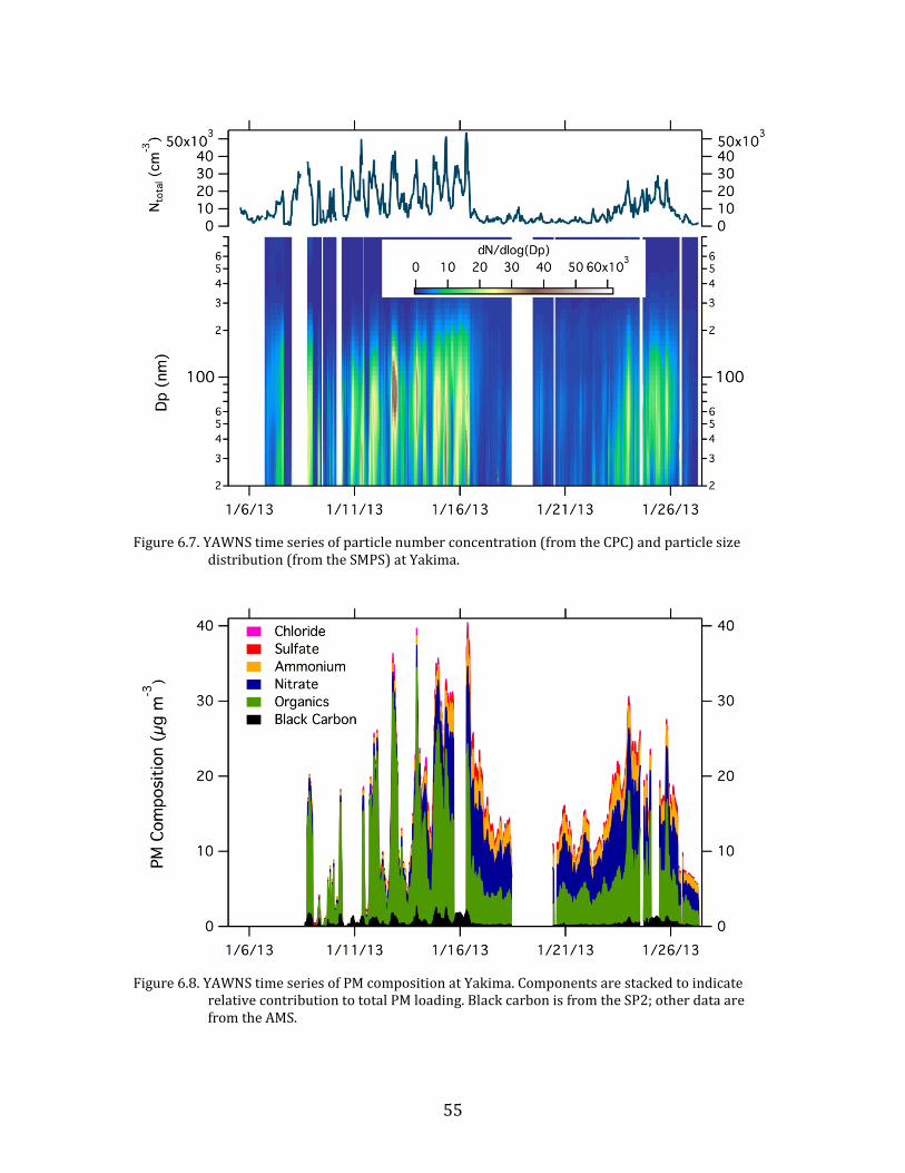
Figure 6.7. YAWNS time series of particle number concentration (from the CPC) and particle size
distribution (from the SMPS) at Yakima.
Figure 6.8. YAWNS time series of PM composition at Yakima. Components are stacked to indicate
relative contribution to total PM loading. Black carbon is from the SP2; other data are from the AMS.
56
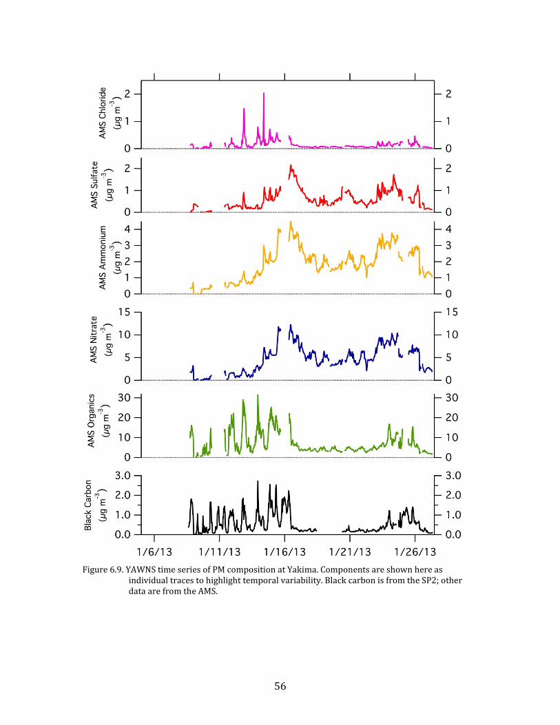
Figure 6.9. YAWNS time series of PM composition at Yakima. Components are shown here as
individual traces to highlight temporal variability. Black carbon is from the SP2; other data are from the AMS.
57
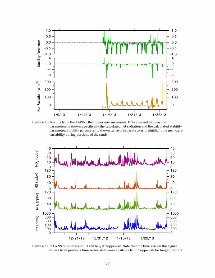
Figure 6.10. Results from the YAWNS flux tower measurements. Only a subset of measured
parameters is shown, specifically the calculated net radiation and the calculated stability parameter. Stability parameter is shown twice of separate axes to highlight the near-zero variability during portions of the study.
Figure 6.11. YAWNS time series of CO and NOx at Toppenish. Note that the time axis on this figure
differs from previous time series; data were available from Toppenish for longer periods.
58
7. Positive Matrix Factorization of PM Organic Composition
The initial analysis of the HR-AMS aerosol composition measurements
reduces the data to produce times series of the major refractory aerosol
components- nitrate, sulfate, ammonium, chloride, and organics. This is done in one
of two ways, depending on whether the unit mass resolution (UMR) or high-
resolution (HR) data are used. Both approaches yield very similar results; in this
report the results presented are based on UMR data. With UMR data, the HR-AMS
signal for each unit mass-to-charge ratio is initially lumped. This means that that
different ions from different source molecules will initially be grouped based on
their common unit mass-to-charge ratio. To separate these contributions, the signal
is redistributed according to a study-specific fragmentation table. The result of this
analysis is the desired first-order product: time series of nitrate, sulfate, ammonium,
chloride, and organics. These results for YAWNS are shown in Figure 6.9.
For the inorganic components, these first-order categories each generally
include the contributions from only one major PM constituent (e.g., nitrate, sulfate,
and ammonium). In contrast, the organics category includes hundreds of
compounds, derived from a variety of primary source types and secondary
atmospheric processes. As such, the information content of the organics category is
somewhat limited. Greater understanding of the organic aerosol can be derived by
conducting a more detailed analysis of the time series of the HR-AMS mass spectral
data within the organics component. The most common approach currently to
accomplish this is via a positive matrix factorization (PMF) analysis on the organic
59
aerosol component of the AMS data (Zhang et al., 2011). Code has been developed
specifically for conducting PMF analysis using HR-AMS organics data (Ulbrich et al.,
2009). Using this code, we have conducted a PMF analysis of the organic aerosol
observed during YAWNS to better understand the sources contributing to PM in
Yakima during winter.
After a detailed evaluation of mass spectral profiles, time series, diurnal
variations, and correlations with external tracers, we selected a four-factor solution
as an appropriate UMR solution for the YAWNS study period. The mass spectra for
the four factors are shown in Figure 7.1. Three of these spectra are consistent with
factors that are regularly found in PMF analyses of HR-AMS data (e.g., Aiken et al.,
2009, 2010; Hildebrandt et al., 2011; Zhang et al., 2011). These factors have been
labeled oxidized organic aerosol (OOA), hydrocarbon-like organic aerosol (HOA),
and biomass burning organic aerosol (BBOA). OOA is characterized mainly by the
strength of the m/z 44 fragment (largely from CO2+), and is frequently treated as a
proxy for secondary organic aerosol. HOA contains much more m/z 43 (from C3H7+)
than 44, and also shows strong signal at m/z 55 and 57 (largely C4H7+ and C4H9+,
respectively), The HOA factor is associated with fresh fossil fuel combustion aerosol.
BBOA contains significant mass spectral contributions from m/z 60 and 73, ions that
are derived from wood smoke (C2H4O2+ and C3H5O2+, respectively). This factor
shows somewhat more variability in the literature, but its presence in the YAWNS
data set is consistent with the prevalence of wood stove emissions in the Yakima
airshed.
60
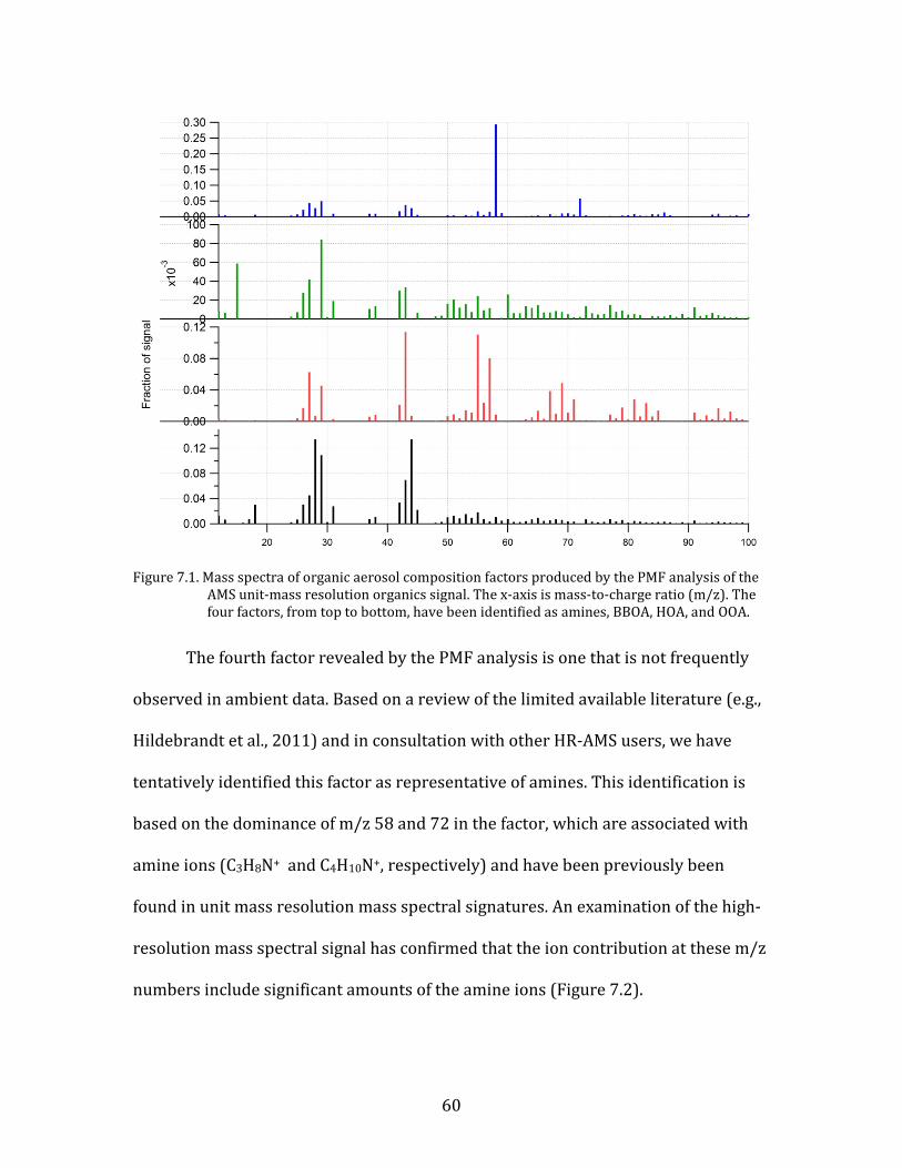
Figure 7.1. Mass spectra of organic aerosol composition factors produced by the PMF analysis of the
AMS unit-mass resolution organics signal. The x-axis is mass-to-charge ratio (m/z). The four factors, from top to bottom, have been identified as amines, BBOA, HOA, and OOA.
The fourth factor revealed by the PMF analysis is one that is not frequently
observed in ambient data. Based on a review of the limited available literature (e.g.,
Hildebrandt et al., 2011) and in consultation with other HR-AMS users, we have
tentatively identified this factor as representative of amines. This identification is
based on the dominance of m/z 58 and 72 in the factor, which are associated with
amine ions (C3H8N+ and C4H10N+, respectively) and have been previously been
found in unit mass resolution mass spectral signatures. An examination of the high-
resolution mass spectral signal has confirmed that the ion contribution at these m/z
numbers include significant amounts of the amine ions (Figure 7.2).
61
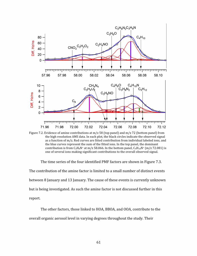
Figure 7.2. Evidence of amine contributions at m/z 58 (top panel) and m/z 72 (bottom panel) from
the high resolution AMS data. In each plot, the black circles indicate the observed signal as a function of m/z. Red curves are fitted contribution from individual labeled ions, and the blue curves represent the sum of the fitted ions. In the top panel, the dominant contribution is from C3H8N+ at m/z 58.066. In the bottom panel, C4H10N+ (m/z 72.081) is one of several ions making significant contributions to the overall observed signal.
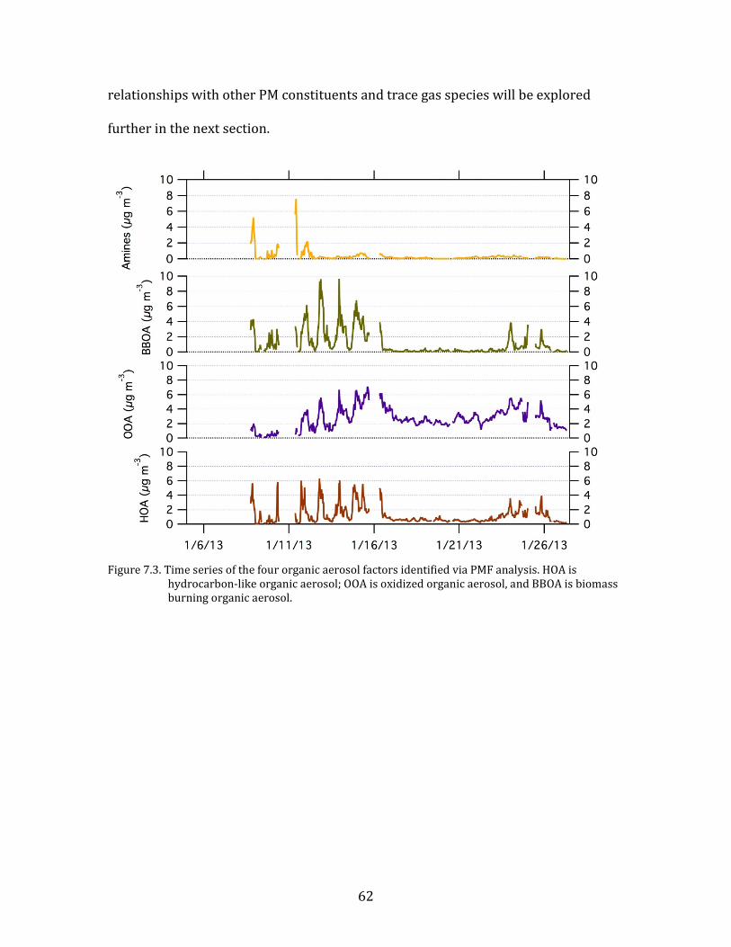
The time series of the four identified PMF factors are shown in Figure 7.3.
The contribution of the amine factor is limited to a small number of distinct events
between 8 January and 13 January. The cause of these events is currently unknown
but is being investigated. As such the amine factor is not discussed further in this
report.
The other factors, those linked to HOA, BBOA, and OOA, contribute to the
overall organic aerosol level in varying degrees throughout the study. Their
62
relationships with other PM constituents and trace gas species will be explored
further in the next section.
Figure 7.3. Time series of the four organic aerosol factors identified via PMF analysis. HOA is
hydrocarbon-like organic aerosol; OOA is oxidized organic aerosol, and BBOA is biomass burning organic aerosol.
63
8. Meteorological and Chemical Drivers of PM Levels
8.1. Classification of Study Periods
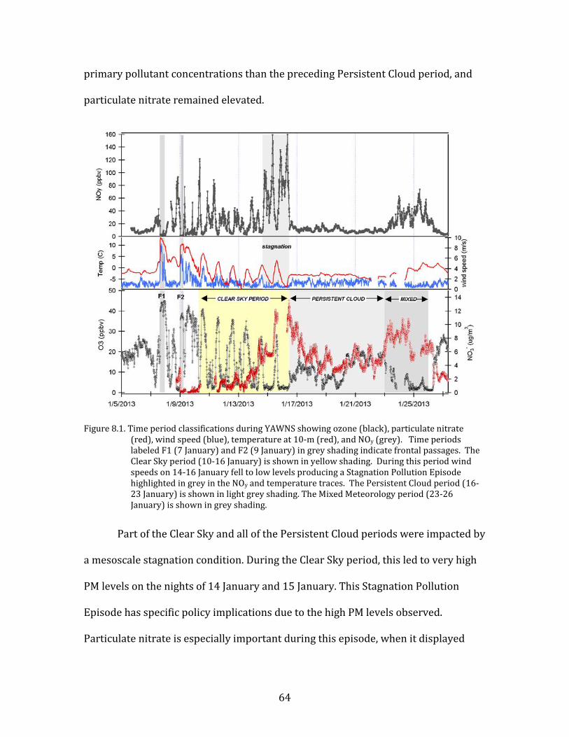
Figure 8.1 shows time period classifications based upon observed
meteorological conditions in Yakima. Frontal passages on 7 January and 9 January
produced strong winds, elevated temperatures, and clean conditions; these events
are noted in the figure. After 9 January, a high pressure condition developed, the
skies cleared, and temperatures began to drop. Our analysis of the meteorological
and chemical drivers of PM episodes in Yakima largely focuses on the contrast
between this clear-sky period and a period the following week that was
characterized by persistent low-level cloud. The beginning of the ‘Clear Sky’ focus
period was chosen to be on the morning of 10 January (07:00). This extended period
has essentially continuous clear skies, a strong diel cycle in temperature, and large
day-to-night variations in boundary layer height that drove strong variations in day-
to-night concentrations of primary pollutants. The end of the Clear Sky period was
the morning of 16 January (07:00). Very soon after this time a cloud layer formed
that persisted for a week; this second period is our ‘Persistent Cloud’ focus period.
This condition was stable beginning at 12:00 on 16 January, and continued until
00:00 on 23 January. This period is notable for the low concentrations and absence
of diel variations for primary pollutants. However, this period also still had elevated
PM2.5 levels. Following the Persistent Cloud period, Yakima experienced a mixed
meteorology condition characterized by broken cloud and somewhat higher
temperatures. This Mixed Meteorology period from 23-26 January had higher
64
primary pollutant concentrations than the preceding Persistent Cloud period, and
particulate nitrate remained elevated.
Figure 8.1. Time period classifications during YAWNS showing ozone (black), particulate nitrate
(red), wind speed (blue), temperature at 10-m (red), and NOy (grey). Time periods labeled F1 (7 January) and F2 (9 January) in grey shading indicate frontal passages. The Clear Sky period (10-16 January) is shown in yellow shading. During this period wind speeds on 14-16 January fell to low levels producing a Stagnation Pollution Episode highlighted in grey in the NOy and temperature traces. The Persistent Cloud period (16-23 January) is shown in light grey shading. The Mixed Meteorology period (23-26 January) is shown in grey shading.
Part of the Clear Sky and all of the Persistent Cloud periods were impacted by
a mesoscale stagnation condition. During the Clear Sky period, this led to very high
PM levels on the nights of 14 January and 15 January. This Stagnation Pollution
Episode has specific policy implications due to the high PM levels observed.
Particulate nitrate is especially important during this episode, when it displayed
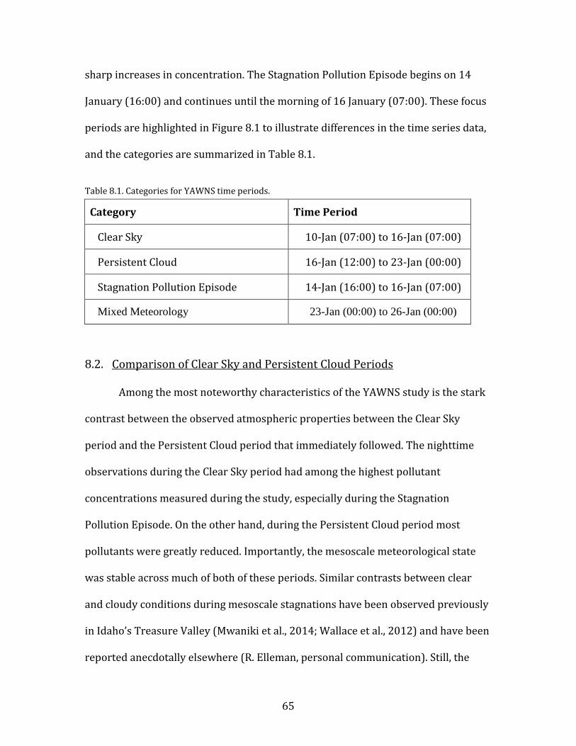
65
sharp increases in concentration. The Stagnation Pollution Episode begins on 14
January (16:00) and continues until the morning of 16 January (07:00). These focus
periods are highlighted in Figure 8.1 to illustrate differences in the time series data,
and the categories are summarized in Table 8.1.
Table 8.1. Categories for YAWNS time periods.
Category Time Period
Clear Sky 10-Jan (07:00) to 16-Jan (07:00)
Persistent Cloud 16-Jan (12:00) to 23-Jan (00:00)
Stagnation Pollution Episode 14-Jan (16:00) to 16-Jan (07:00)
Mixed Meteorology 23-Jan (00:00) to 26-Jan (00:00)
8.2. Comparison of Clear Sky and Persistent Cloud Periods
Among the most noteworthy characteristics of the YAWNS study is the stark
contrast between the observed atmospheric properties between the Clear Sky
period and the Persistent Cloud period that immediately followed. The nighttime
observations during the Clear Sky period had among the highest pollutant
concentrations measured during the study, especially during the Stagnation
Pollution Episode. On the other hand, during the Persistent Cloud period most
pollutants were greatly reduced. Importantly, the mesoscale meteorological state
was stable across much of both of these periods. Similar contrasts between clear
and cloudy conditions during mesoscale stagnations have been observed previously
in Idaho’s Treasure Valley (Mwaniki et al., 2014; Wallace et al., 2012) and have been
reported anecdotally elsewhere (R. Elleman, personal communication). Still, the
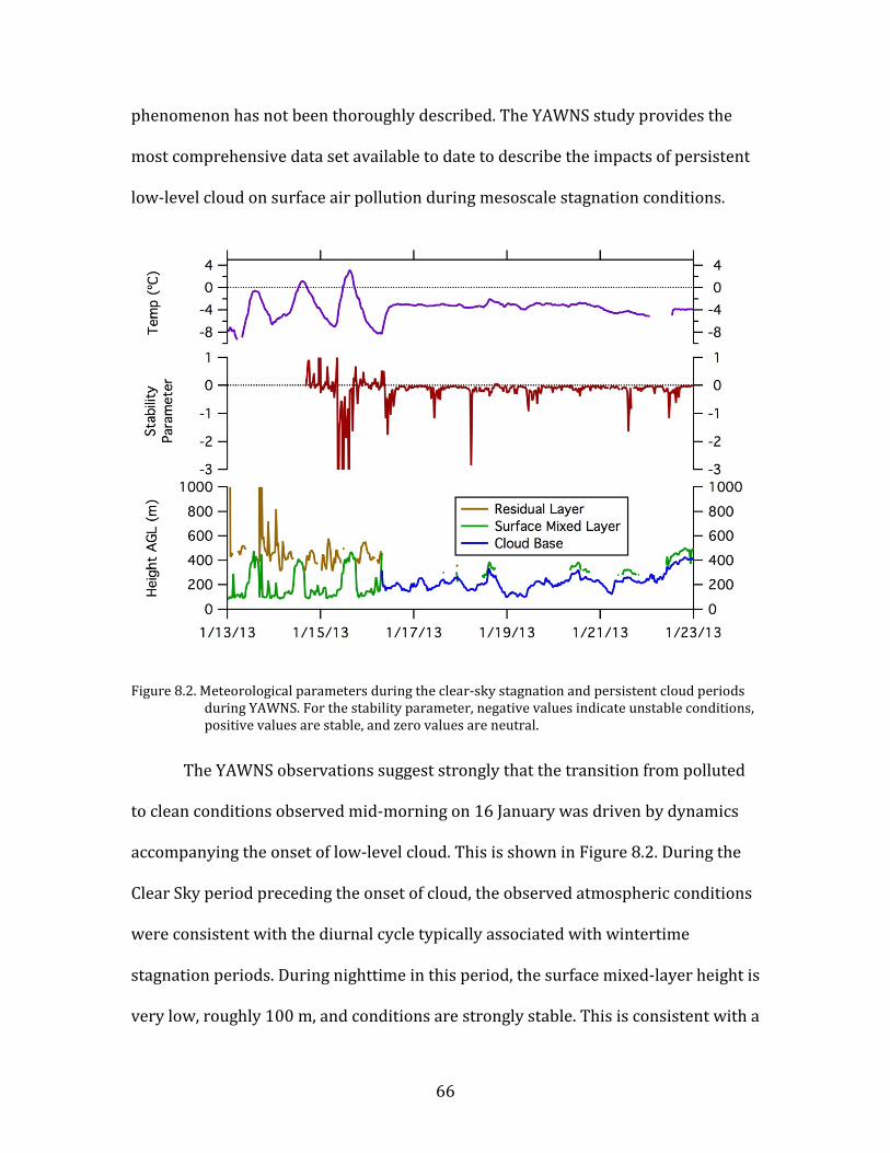
66
phenomenon has not been thoroughly described. The YAWNS study provides the
most comprehensive data set available to date to describe the impacts of persistent
low-level cloud on surface air pollution during mesoscale stagnation conditions.
Figure 8.2. Meteorological parameters during the clear-sky stagnation and persistent cloud periods during YAWNS. For the stability parameter, negative values indicate unstable conditions, positive values are stable, and zero values are neutral.
The YAWNS observations suggest strongly that the transition from polluted
to clean conditions observed mid-morning on 16 January was driven by dynamics
accompanying the onset of low-level cloud. This is shown in Figure 8.2. During the
Clear Sky period preceding the onset of cloud, the observed atmospheric conditions
were consistent with the diurnal cycle typically associated with wintertime
stagnation periods. During nighttime in this period, the surface mixed-layer height is
very low, roughly 100 m, and conditions are strongly stable. This is consistent with a
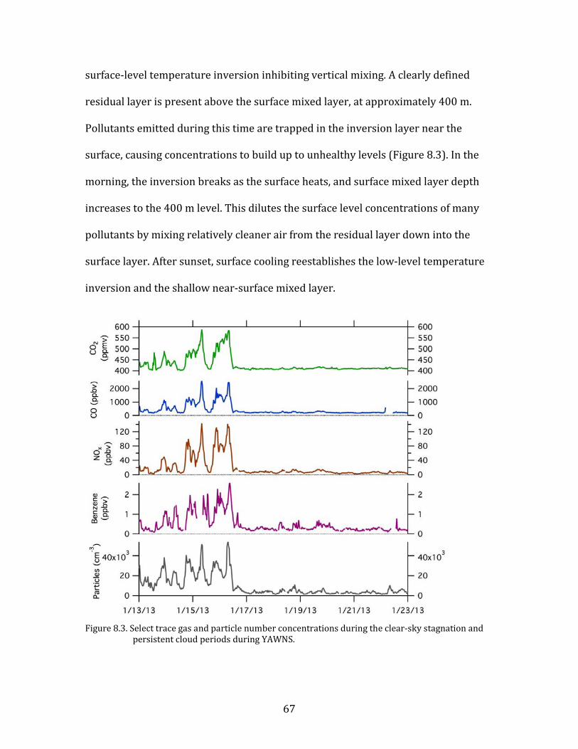
67
surface-level temperature inversion inhibiting vertical mixing. A clearly defined
residual layer is present above the surface mixed layer, at approximately 400 m.
Pollutants emitted during this time are trapped in the inversion layer near the
surface, causing concentrations to build up to unhealthy levels (Figure 8.3). In the
morning, the inversion breaks as the surface heats, and surface mixed layer depth
increases to the 400 m level. This dilutes the surface level concentrations of many
pollutants by mixing relatively cleaner air from the residual layer down into the
surface layer. After sunset, surface cooling reestablishes the low-level temperature
inversion and the shallow near-surface mixed layer.
Figure 8.3. Select trace gas and particle number concentrations during the clear-sky stagnation and
persistent cloud periods during YAWNS.
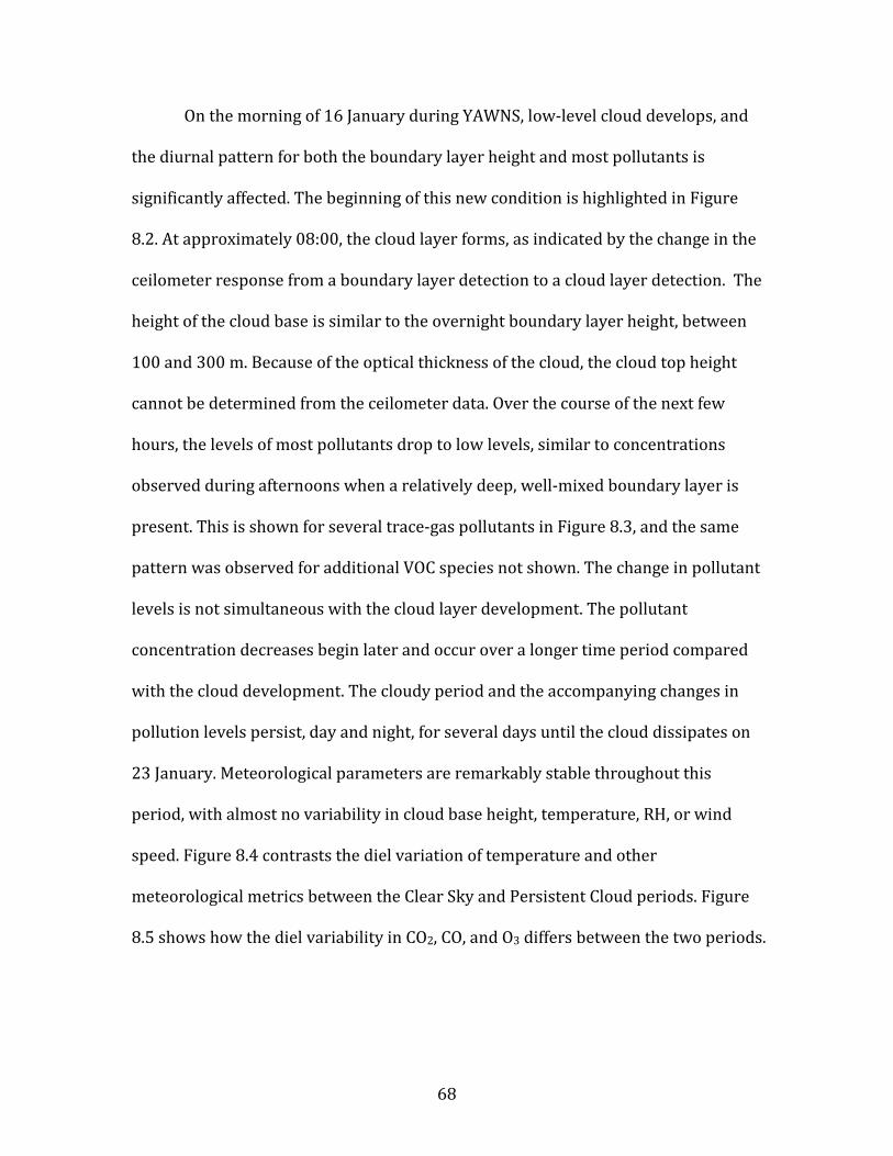
68
On the morning of 16 January during YAWNS, low-level cloud develops, and
the diurnal pattern for both the boundary layer height and most pollutants is
significantly affected. The beginning of this new condition is highlighted in Figure
8.2. At approximately 08:00, the cloud layer forms, as indicated by the change in the
ceilometer response from a boundary layer detection to a cloud layer detection. The
height of the cloud base is similar to the overnight boundary layer height, between
100 and 300 m. Because of the optical thickness of the cloud, the cloud top height
cannot be determined from the ceilometer data. Over the course of the next few
hours, the levels of most pollutants drop to low levels, similar to concentrations
observed during afternoons when a relatively deep, well-mixed boundary layer is
present. This is shown for several trace-gas pollutants in Figure 8.3, and the same
pattern was observed for additional VOC species not shown. The change in pollutant
levels is not simultaneous with the cloud layer development. The pollutant
concentration decreases begin later and occur over a longer time period compared
with the cloud development. The cloudy period and the accompanying changes in
pollution levels persist, day and night, for several days until the cloud dissipates on
23 January. Meteorological parameters are remarkably stable throughout this
period, with almost no variability in cloud base height, temperature, RH, or wind
speed. Figure 8.4 contrasts the diel variation of temperature and other
meteorological metrics between the Clear Sky and Persistent Cloud periods. Figure
8.5 shows how the diel variability in CO2, CO, and O3 differs between the two periods.
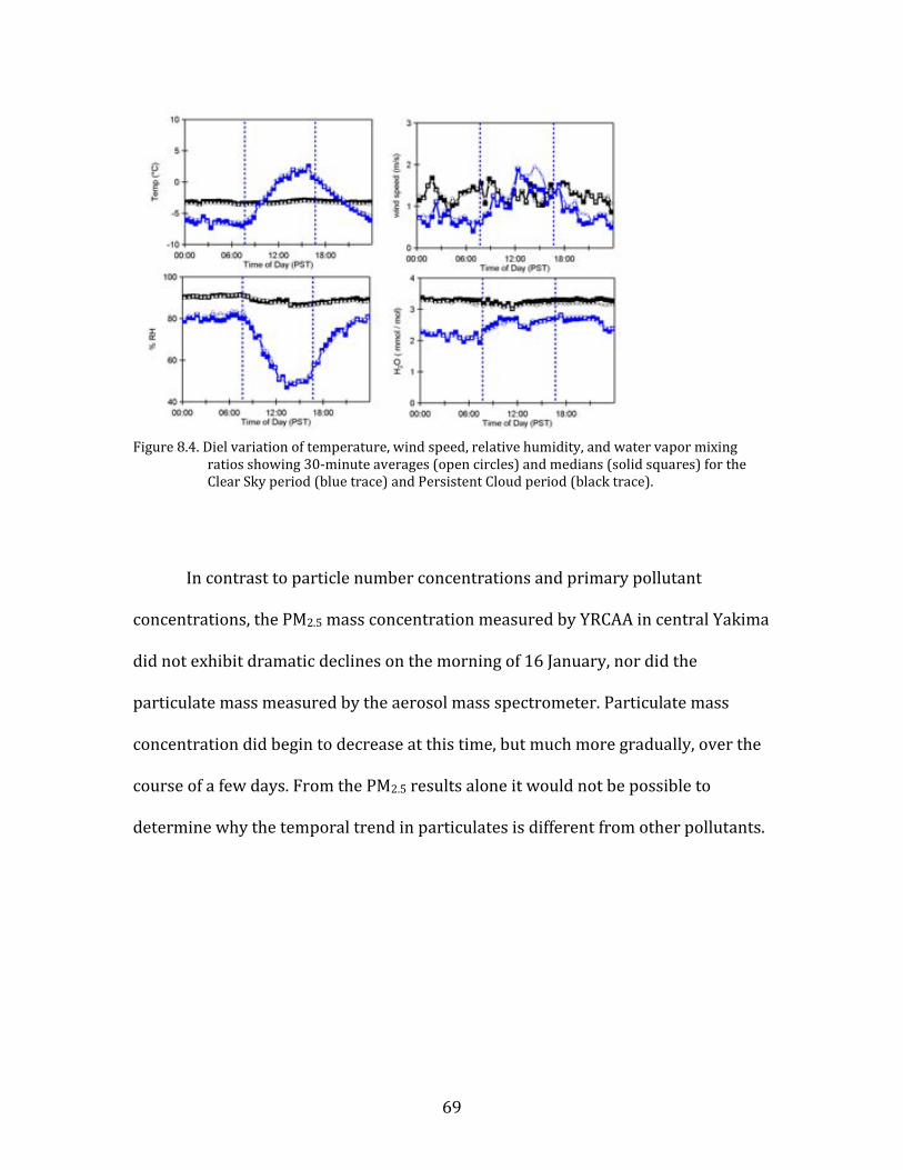
69
Figure 8.4. Diel variation of temperature, wind speed, relative humidity, and water vapor mixing
ratios showing 30-minute averages (open circles) and medians (solid squares) for the Clear Sky period (blue trace) and Persistent Cloud period (black trace).
In contrast to particle number concentrations and primary pollutant
concentrations, the PM2.5 mass concentration measured by YRCAA in central Yakima
did not exhibit dramatic declines on the morning of 16 January, nor did the
particulate mass measured by the aerosol mass spectrometer. Particulate mass
concentration did begin to decrease at this time, but much more gradually, over the
course of a few days. From the PM2.5 results alone it would not be possible to
determine why the temporal trend in particulates is different from other pollutants.
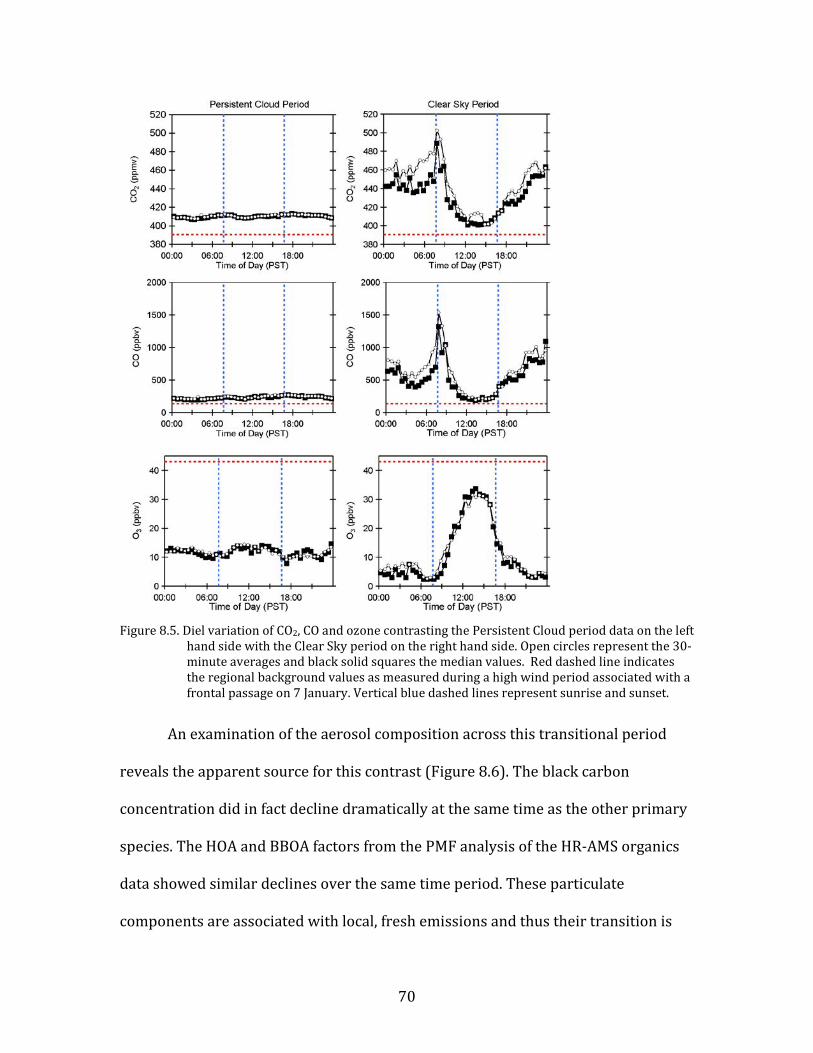
70
Figure 8.5. Diel variation of CO2, CO and ozone contrasting the Persistent Cloud period data on the left
hand side with the Clear Sky period on the right hand side. Open circles represent the 30-minute averages and black solid squares the median values. Red dashed line indicates the regional background values as measured during a high wind period associated with a frontal passage on 7 January. Vertical blue dashed lines represent sunrise and sunset.
An examination of the aerosol composition across this transitional period
reveals the apparent source for this contrast (Figure 8.6). The black carbon
concentration did in fact decline dramatically at the same time as the other primary
species. The HOA and BBOA factors from the PMF analysis of the HR-AMS organics
data showed similar declines over the same time period. These particulate
components are associated with local, fresh emissions and thus their transition is
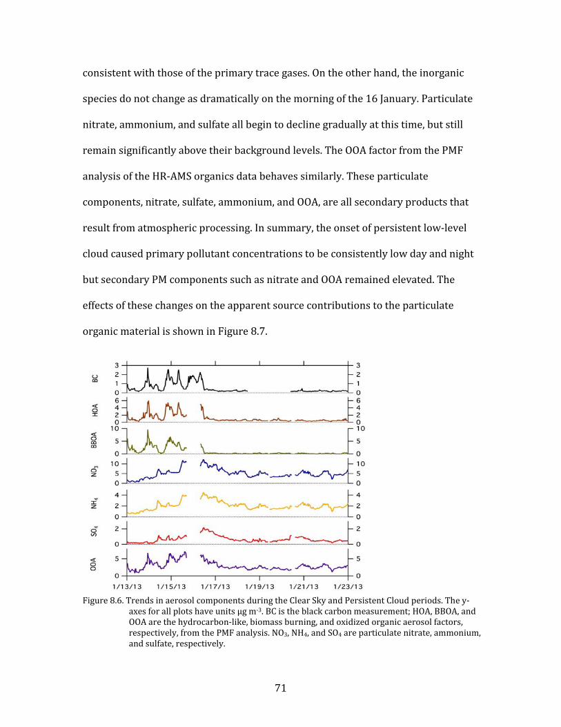
71
consistent with those of the primary trace gases. On the other hand, the inorganic
species do not change as dramatically on the morning of the 16 January. Particulate
nitrate, ammonium, and sulfate all begin to decline gradually at this time, but still
remain significantly above their background levels. The OOA factor from the PMF
analysis of the HR-AMS organics data behaves similarly. These particulate
components, nitrate, sulfate, ammonium, and OOA, are all secondary products that
result from atmospheric processing. In summary, the onset of persistent low-level
cloud caused primary pollutant concentrations to be consistently low day and night
but secondary PM components such as nitrate and OOA remained elevated. The
effects of these changes on the apparent source contributions to the particulate
organic material is shown in Figure 8.7.
Figure 8.6. Trends in aerosol components during the Clear Sky and Persistent Cloud periods. The y-
axes for all plots have units µg m-3. BC is the black carbon measurement; HOA, BBOA, and OOA are the hydrocarbon-like, biomass burning, and oxidized organic aerosol factors, respectively, from the PMF analysis. NO3, NH4, and SO4 are particulate nitrate, ammonium, and sulfate, respectively.
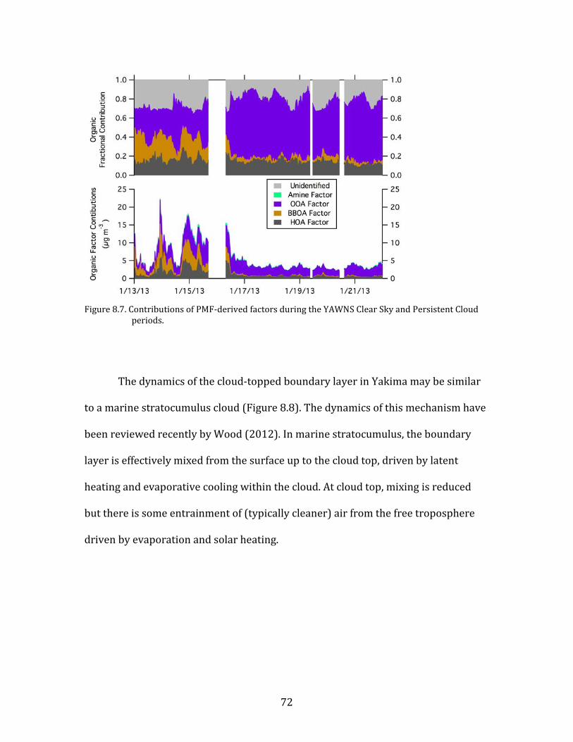
72
Figure 8.7. Contributions of PMF-derived factors during the YAWNS Clear Sky and Persistent Cloud
periods.
The dynamics of the cloud-topped boundary layer in Yakima may be similar
to a marine stratocumulus cloud (Figure 8.8). The dynamics of this mechanism have
been reviewed recently by Wood (2012). In marine stratocumulus, the boundary
layer is effectively mixed from the surface up to the cloud top, driven by latent
heating and evaporative cooling within the cloud. At cloud top, mixing is reduced
but there is some entrainment of (typically cleaner) air from the free troposphere
driven by evaporation and solar heating.
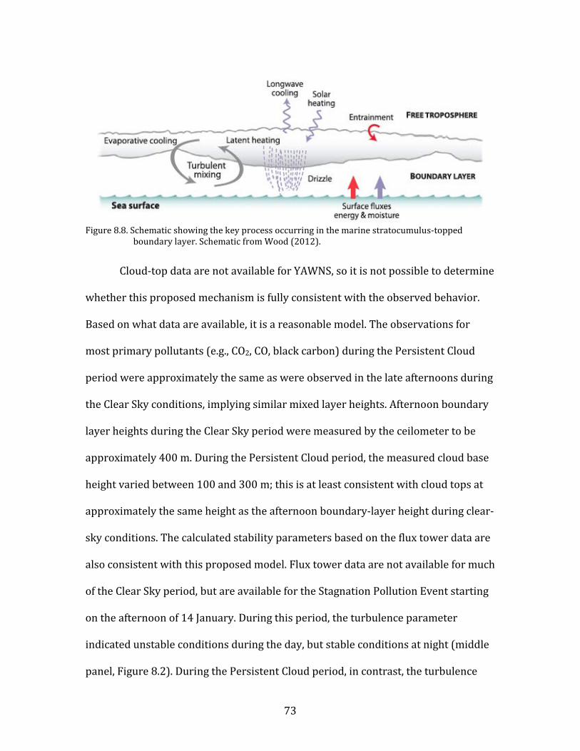
73
Figure 8.8. Schematic showing the key process occurring in the marine stratocumulus-topped
boundary layer. Schematic from Wood (2012).
Cloud-top data are not available for YAWNS, so it is not possible to determine
whether this proposed mechanism is fully consistent with the observed behavior.
Based on what data are available, it is a reasonable model. The observations for
most primary pollutants (e.g., CO2, CO, black carbon) during the Persistent Cloud
period were approximately the same as were observed in the late afternoons during
the Clear Sky conditions, implying similar mixed layer heights. Afternoon boundary
layer heights during the Clear Sky period were measured by the ceilometer to be
approximately 400 m. During the Persistent Cloud period, the measured cloud base
height varied between 100 and 300 m; this is at least consistent with cloud tops at
approximately the same height as the afternoon boundary-layer height during clear-
sky conditions. The calculated stability parameters based on the flux tower data are
also consistent with this proposed model. Flux tower data are not available for much
of the Clear Sky period, but are available for the Stagnation Pollution Event starting
on the afternoon of 14 January. During this period, the turbulence parameter
indicated unstable conditions during the day, but stable conditions at night (middle
panel, Figure 8.2). During the Persistent Cloud period, in contrast, the turbulence
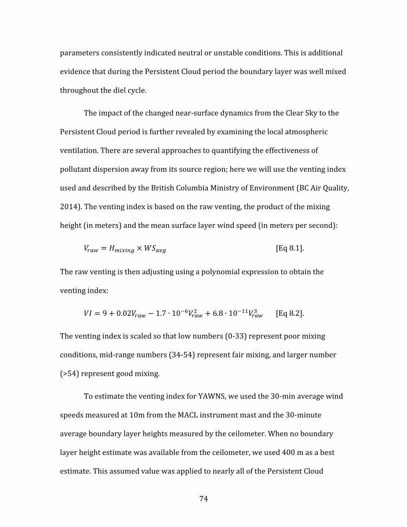
74
parameters consistently indicated neutral or unstable conditions. This is additional
evidence that during the Persistent Cloud period the boundary layer was well mixed
throughout the diel cycle.
The impact of the changed near-surface dynamics from the Clear Sky to the
Persistent Cloud period is further revealed by examining the local atmospheric
ventilation. There are several approaches to quantifying the effectiveness of
pollutant dispersion away from its source region; here we will use the venting index
used and described by the British Columbia Ministry of Environment (BC Air Quality,
2014). The venting index is based on the raw venting, the product of the mixing
height (in meters) and the mean surface layer wind speed (in meters per second):
𝑉𝑟𝑎𝑤 = 𝐻𝑚𝑖𝑥𝑖𝑛𝑔 × 𝑊𝑆𝑎𝑣𝑔 [Eq 8.1].
The raw venting is then adjusting using a polynomial expression to obtain the
venting index:
𝑉𝐼 = 9 + 0.02𝑉𝑟𝑎𝑤 − 1.7 ∙ 10−6𝑉𝑟𝑎𝑤2 + 6.8 ∙ 10−11𝑉𝑟𝑎𝑤
3 [Eq 8.2].
The venting index is scaled so that low numbers (0-33) represent poor mixing
conditions, mid-range numbers (34-54) represent fair mixing, and larger number
(>54) represent good mixing.
To estimate the venting index for YAWNS, we used the 30-min average wind
speeds measured at 10m from the MACL instrument mast and the 30-minute
average boundary layer heights measured by the ceilometer. When no boundary
layer height estimate was available from the ceilometer, we used 400 m as a best
estimate. This assumed value was applied to nearly all of the Persistent Cloud
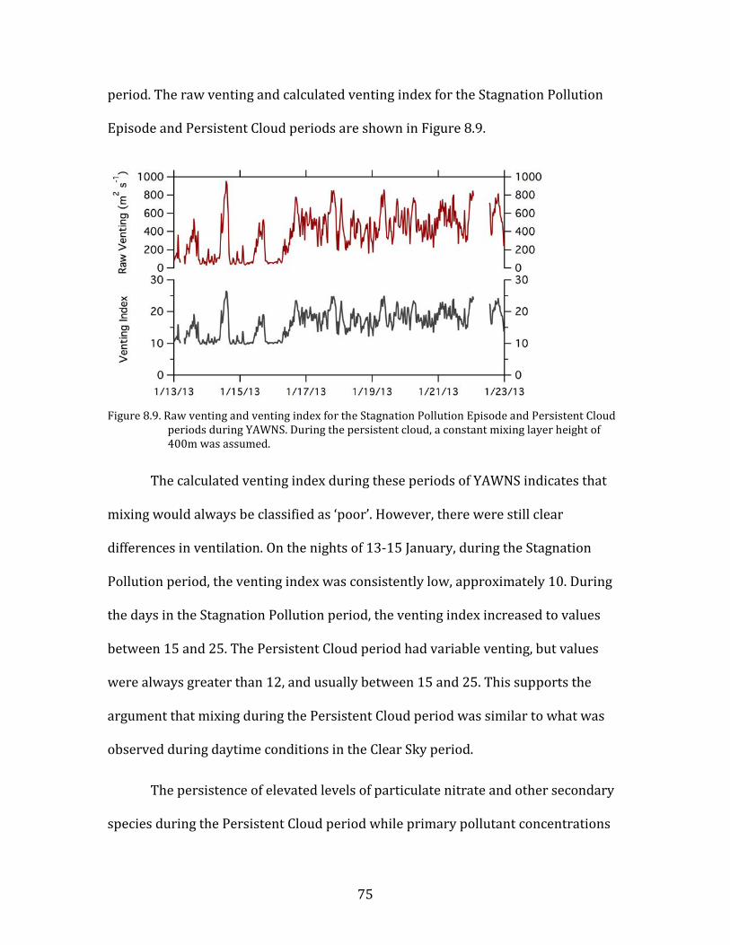
75
period. The raw venting and calculated venting index for the Stagnation Pollution
Episode and Persistent Cloud periods are shown in Figure 8.9.
Figure 8.9. Raw venting and venting index for the Stagnation Pollution Episode and Persistent Cloud
periods during YAWNS. During the persistent cloud, a constant mixing layer height of 400m was assumed.
The calculated venting index during these periods of YAWNS indicates that
mixing would always be classified as ‘poor’. However, there were still clear
differences in ventilation. On the nights of 13-15 January, during the Stagnation
Pollution period, the venting index was consistently low, approximately 10. During
the days in the Stagnation Pollution period, the venting index increased to values
between 15 and 25. The Persistent Cloud period had variable venting, but values
were always greater than 12, and usually between 15 and 25. This supports the
argument that mixing during the Persistent Cloud period was similar to what was
observed during daytime conditions in the Clear Sky period.
The persistence of elevated levels of particulate nitrate and other secondary
species during the Persistent Cloud period while primary pollutant concentrations
76
decline is not readily explained. This persistence could be a result of enhanced
secondary pollutant production during the cloudy period, or could arise from less
effective ventilation of secondary species. Possible mechanisms for these observed
phenomena are discussed in the following sections.
8.3. Neutralization State of Major Particulate Inorganic Ions
The amount of nitrate in the particle phase depends in large part on the
amount of ammonium available to neutralize nitric acid. However, ammonium
reacts preferentially to neutralize sulfate species first, and so the amount of sulfate
available must also be considered to determine how much ammonium remains to
react with nitrate. In most cases, if there is sufficient ammonium to neutralize any
available sulfate, then overall full neutralization would be expected. After sulfate
neutralization, any remaining ammonium would generally co-condense with nitrate
(and vice versa), yielding a neutralized particle phase. However, in cases of cold
temperatures and/or high humidity, it is possible for some unneutralized ammonia
or nitric acid to condense to produce a basic or acidic aerosol (Mwaniki et al., 2014).
To evaluate the degree of neutralization of these major inorganic aerosol
species during YAWNS, we compared the amounts of ammonium, nitrate, and
sulfate on a molar basis. The mass-based composition data from the HR-AMS were
first converted to molar concentrations using the ionic masses: 18.04, 62.01, and
96.07 µg/µmol for ammonium, nitrate, and sulfate, respectively. The results are
shown in the bottom panel of Figure 8.10. As expected, nitrate and ammonium
dominate the inorganic composition on a molar basis, both being approximately an
order of magnitude greater than the sulfate concentration. We then used the sulfate
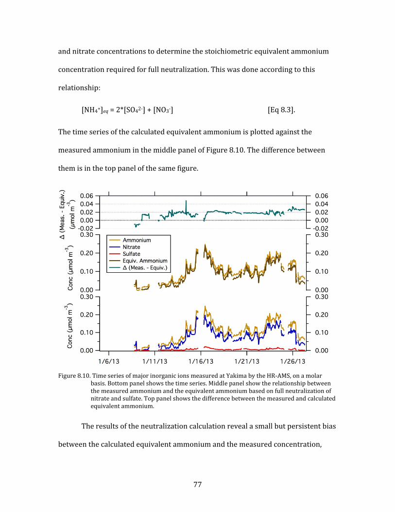
77
and nitrate concentrations to determine the stoichiometric equivalent ammonium
concentration required for full neutralization. This was done according to this
relationship:
[NH4+]eq = 2*[SO42-] + [NO3-] [Eq 8.3].
The time series of the calculated equivalent ammonium is plotted against the
measured ammonium in the middle panel of Figure 8.10. The difference between
them is in the top panel of the same figure.
Figure 8.10. Time series of major inorganic ions measured at Yakima by the HR-AMS, on a molar
basis. Bottom panel shows the time series. Middle panel show the relationship between the measured ammonium and the equivalent ammonium based on full neutralization of nitrate and sulfate. Top panel shows the difference between the measured and calculated equivalent ammonium.
The results of the neutralization calculation reveal a small but persistent bias
between the calculated equivalent ammonium and the measured concentration,
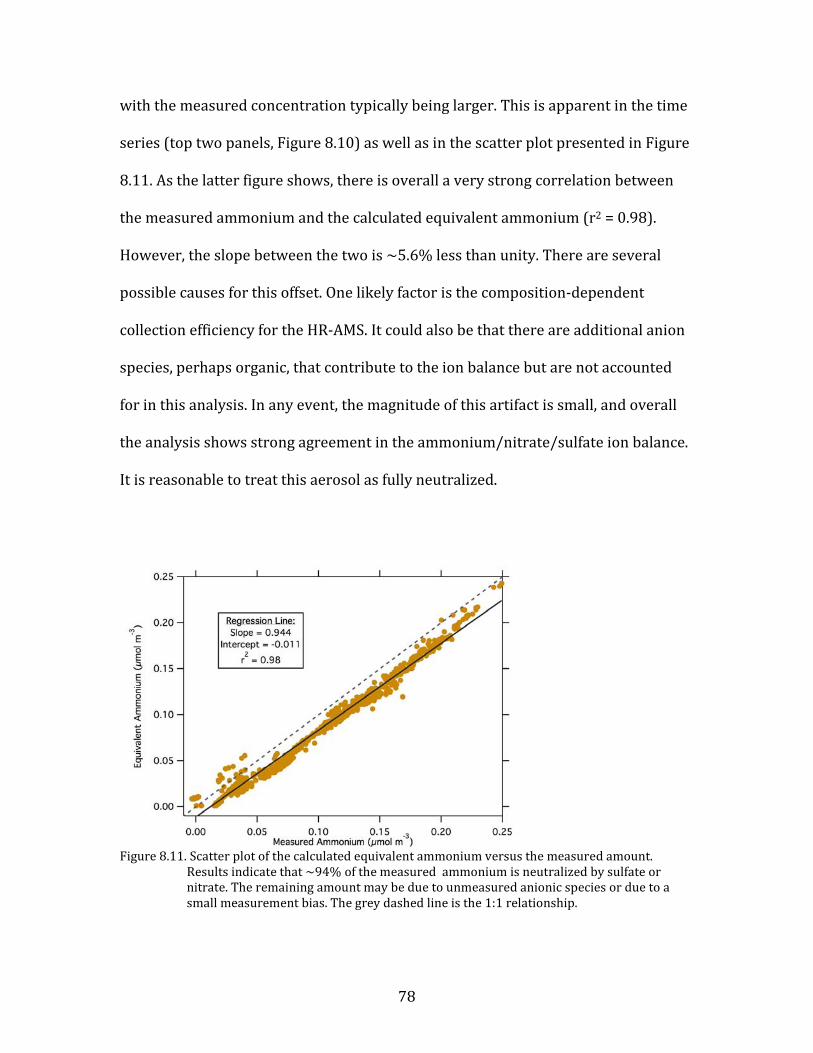
78
with the measured concentration typically being larger. This is apparent in the time
series (top two panels, Figure 8.10) as well as in the scatter plot presented in Figure
8.11. As the latter figure shows, there is overall a very strong correlation between
the measured ammonium and the calculated equivalent ammonium (r2 = 0.98).
However, the slope between the two is ~5.6% less than unity. There are several
possible causes for this offset. One likely factor is the composition-dependent
collection efficiency for the HR-AMS. It could also be that there are additional anion
species, perhaps organic, that contribute to the ion balance but are not accounted
for in this analysis. In any event, the magnitude of this artifact is small, and overall
the analysis shows strong agreement in the ammonium/nitrate/sulfate ion balance.
It is reasonable to treat this aerosol as fully neutralized.
Figure 8.11. Scatter plot of the calculated equivalent ammonium versus the measured amount.
Results indicate that ~94% of the measured ammonium is neutralized by sulfate or nitrate. The remaining amount may be due to unmeasured anionic species or due to a small measurement bias. The grey dashed line is the 1:1 relationship.
79
8.4. Potential Causes of Observed Particulate Nitrate Levels at Yakima
The major motivation of the YAWNS study was to need to understand the
causes of the observed particulate nitrate levels during wintertime in the upper
Yakima Valley. Fundamentally, particulate nitrate loads are always driven primarily
by three factors: meteorology, and the availability of ammonia and nitrate
precursors. How these factors interrelate and the influence of additional secondary
factors can vary and are the focus of this discussion.
The role of meteorology in influencing particulate nitrate formation cannot
be ignored. Particulate ammonium nitrate exists in chemical equilibrium with
ammonia and nitric acid in the gas phase. In summer, when temperatures are warm,
the equilibrium is shifted toward the gas phase, and there is little nitrate present in
particulate form. However, at the cold temperatures present in Yakima during
winter, the gas-particle equilibrium is heavily shifted toward the particle phase.
While that basic concept is straightforward, the full details of the ammonium nitrate
equilibrium relationship are complex. In addition to temperature, there are
dependencies on relative humidity and the full aerosol composition. Additionally,
the levels of nitric acid and ammonia in the atmosphere depend strongly on the gas-
phase chemistry of these species, which have additional meteorological
dependencies. A full analysis of this system is beyond the scope of this project, but
simplified conceptual model can inform our understanding of the situation in
Yakima during winter.
80
In an idealized system consisting only of ammonia and nitric acid in dry air,
the equilibrium between the gas and particle phase can be described by reaction
8.1:
NH3 (g) + HNO3 (g) NH4NO3 (s) [R 8.1].
The dissociation expression associated with this reaction is:
𝐾𝑝(𝑇) = 𝑝𝑁𝐻3𝑝𝐻𝑁𝑂3 [Eqn. 8.4],
where pNH3 and pHNO3 are the partial pressures of ammonia and nitric acid,
respectively, expressed in units of ppbv (at sea-level pressure). The value of the
equilibrium dissociation constant, Kp(T), is a strong function of temperature
(Seinfeld & Pandis, 2006):
ln 𝐾𝑝 = 84.6 − 24220𝑇
− 6.1 ln � 𝑇298
� [Eqn. 8.5].
Here, temperature (T) is in Kelvin. The value of Kp(T) for YAWNS is provided in
Figure 8.12. During the warmest part of the study it reaches a maximum value of 1.2
ppb2, but during Clear Sky period it was 0.1 or below, and during the Persistent
Cloudy period its value was approximately 0.01. These values should be treated as
the maximum gas phase product for NH3 and HNO3 at any given time, since the
presence of other substances, including water, would tend to force more of the
ammonia and nitric acid into the condensed phase.
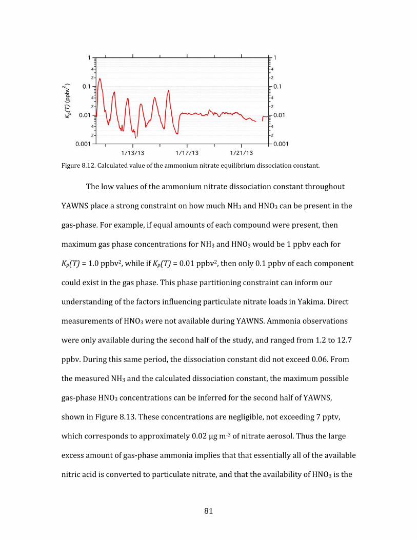
81
Figure 8.12. Calculated value of the ammonium nitrate equilibrium dissociation constant.
The low values of the ammonium nitrate dissociation constant throughout
YAWNS place a strong constraint on how much NH3 and HNO3 can be present in the
gas-phase. For example, if equal amounts of each compound were present, then
maximum gas phase concentrations for NH3 and HNO3 would be 1 ppbv each for
Kp(T) = 1.0 ppbv2, while if Kp(T) = 0.01 ppbv2, then only 0.1 ppbv of each component
could exist in the gas phase. This phase partitioning constraint can inform our
understanding of the factors influencing particulate nitrate loads in Yakima. Direct
measurements of HNO3 were not available during YAWNS. Ammonia observations
were only available during the second half of the study, and ranged from 1.2 to 12.7
ppbv. During this same period, the dissociation constant did not exceed 0.06. From
the measured NH3 and the calculated dissociation constant, the maximum possible
gas-phase HNO3 concentrations can be inferred for the second half of YAWNS,
shown in Figure 8.13. These concentrations are negligible, not exceeding 7 pptv,
which corresponds to approximately 0.02 µg m-3 of nitrate aerosol. Thus the large
excess amount of gas-phase ammonia implies that that essentially all of the available
nitric acid is converted to particulate nitrate, and that the availability of HNO3 is the
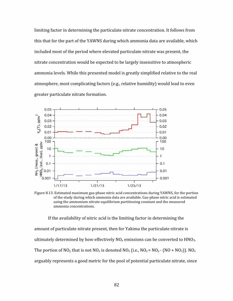
82
limiting factor in determining the particulate nitrate concentration. It follows from
this that for the part of the YAWNS during which ammonia data are available, which
included most of the period where elevated particulate nitrate was present, the
nitrate concentration would be expected to be largely insensitive to atmospheric
ammonia levels. While this presented model is greatly simplified relative to the real
atmosphere, most complicating factors (e.g., relative humidity) would lead to even
greater particulate nitrate formation.
Figure 8.13. Estimated maximum gas-phase nitric acid concentrations during YAWNS, for the portion
of the study during which ammonia data are available. Gas-phase nitric acid is estimated using the ammonium nitrate equilibrium partitioning constant and the measured ammonia concentrations.
If the availability of nitric acid is the limiting factor in determining the
amount of particulate nitrate present, then for Yakima the particulate nitrate is
ultimately determined by how effectively NOx emissions can be converted to HNO3.
The portion of NOy that is not NOx is denoted NOz (i.e., NOz = NOy - (NO + NO2)). NOz
arguably represents a good metric for the pool of potential particulate nitrate, since
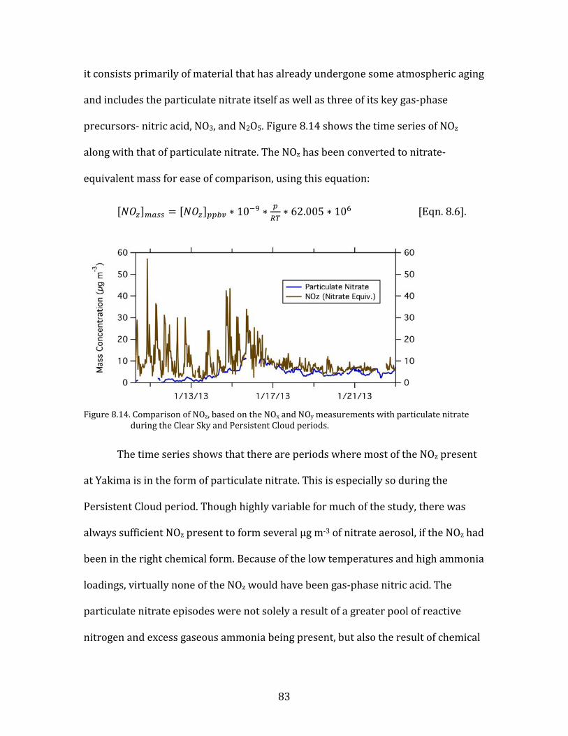
83
it consists primarily of material that has already undergone some atmospheric aging
and includes the particulate nitrate itself as well as three of its key gas-phase
precursors- nitric acid, NO3, and N2O5. Figure 8.14 shows the time series of NOz
along with that of particulate nitrate. The NOz has been converted to nitrate-
equivalent mass for ease of comparison, using this equation:
[𝑁𝑂𝑧]𝑚𝑎𝑠𝑠 = [𝑁𝑂𝑧]𝑝𝑝𝑏𝑣 ∗ 10−9 ∗ 𝑝𝑅𝑇
∗ 62.005 ∗ 106 [Eqn. 8.6].
Figure 8.14. Comparison of NOz, based on the NOx and NOy measurements with particulate nitrate
during the Clear Sky and Persistent Cloud periods.
The time series shows that there are periods where most of the NOz present
at Yakima is in the form of particulate nitrate. This is especially so during the
Persistent Cloud period. Though highly variable for much of the study, there was
always sufficient NOz present to form several µg m-3 of nitrate aerosol, if the NOz had
been in the right chemical form. Because of the low temperatures and high ammonia
loadings, virtually none of the NOz would have been gas-phase nitric acid. The
particulate nitrate episodes were not solely a result of a greater pool of reactive
nitrogen and excess gaseous ammonia being present, but also the result of chemical
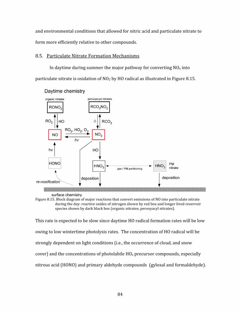
84
and environmental conditions that allowed for nitric acid and particulate nitrate to
form more efficiently relative to other compounds.
8.5. Particulate Nitrate Formation Mechanisms
In daytime during summer the major pathway for converting NOx into
particulate nitrate is oxidation of NO2 by HO radical as illustrated in Figure 8.15.
Figure 8.15. Block diagram of major reactions that convert emissions of NO into particulate nitrate
during the day: reactive oxides of nitrogen shown by red box and longer lived reservoir species shown by dark black box (organic nitrates, peroxyacyl nitrates).
This rate is expected to be slow since daytime HO radical formation rates will be low
owing to low wintertime photolysis rates. The concentration of HO radical will be
strongly dependent on light conditions (i.e., the occurrence of cloud, and snow
cover) and the concentrations of photolabile HOx precursor compounds, especially
nitrous acid (HONO) and primary aldehyde compounds (gyloxal and formaldehyde).
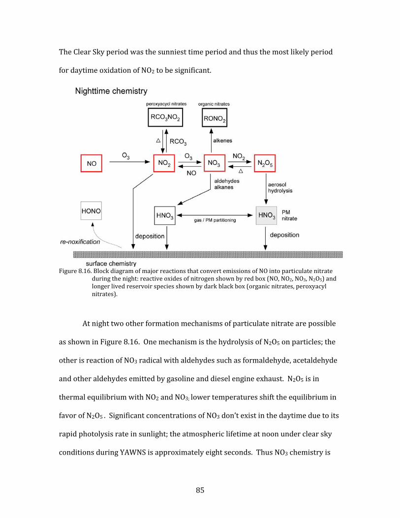
85
The Clear Sky period was the sunniest time period and thus the most likely period
for daytime oxidation of NO2 to be significant.
Figure 8.16. Block diagram of major reactions that convert emissions of NO into particulate nitrate
during the night: reactive oxides of nitrogen shown by red box (NO, NO2, NO3, N2O5) and longer lived reservoir species shown by dark black box (organic nitrates, peroxyacyl nitrates).
At night two other formation mechanisms of particulate nitrate are possible
as shown in Figure 8.16. One mechanism is the hydrolysis of N2O5 on particles; the
other is reaction of NO3 radical with aldehydes such as formaldehyde, acetaldehyde
and other aldehydes emitted by gasoline and diesel engine exhaust. N2O5 is in
thermal equilibrium with NO2 and NO3; lower temperatures shift the equilibrium in
favor of N2O5 . Significant concentrations of NO3 don’t exist in the daytime due to its
rapid photolysis rate in sunlight; the atmospheric lifetime at noon under clear sky
conditions during YAWNS is approximately eight seconds. Thus NO3 chemistry is
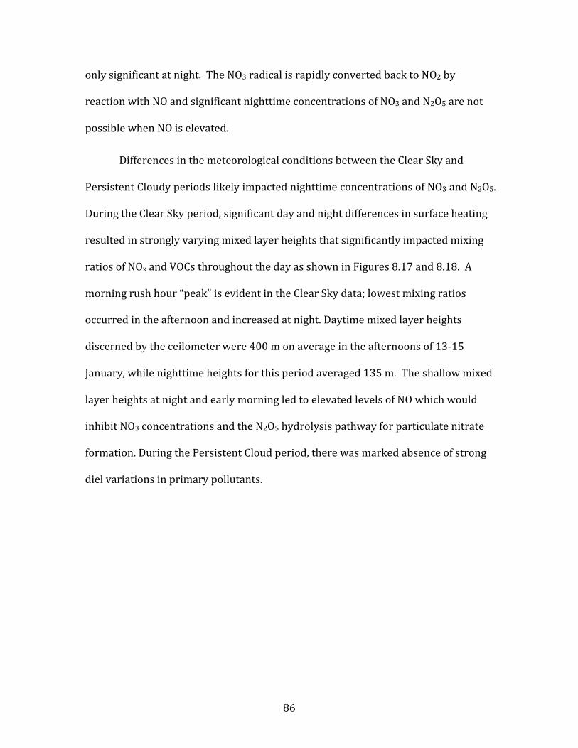
86
only significant at night. The NO3 radical is rapidly converted back to NO2 by
reaction with NO and significant nighttime concentrations of NO3 and N2O5 are not
possible when NO is elevated.
Differences in the meteorological conditions between the Clear Sky and
Persistent Cloudy periods likely impacted nighttime concentrations of NO3 and N2O5.
During the Clear Sky period, significant day and night differences in surface heating
resulted in strongly varying mixed layer heights that significantly impacted mixing
ratios of NOx and VOCs throughout the day as shown in Figures 8.17 and 8.18. A
morning rush hour “peak” is evident in the Clear Sky data; lowest mixing ratios
occurred in the afternoon and increased at night. Daytime mixed layer heights
discerned by the ceilometer were 400 m on average in the afternoons of 13-15
January, while nighttime heights for this period averaged 135 m. The shallow mixed
layer heights at night and early morning led to elevated levels of NO which would
inhibit NO3 concentrations and the N2O5 hydrolysis pathway for particulate nitrate
formation. During the Persistent Cloud period, there was marked absence of strong
diel variations in primary pollutants.
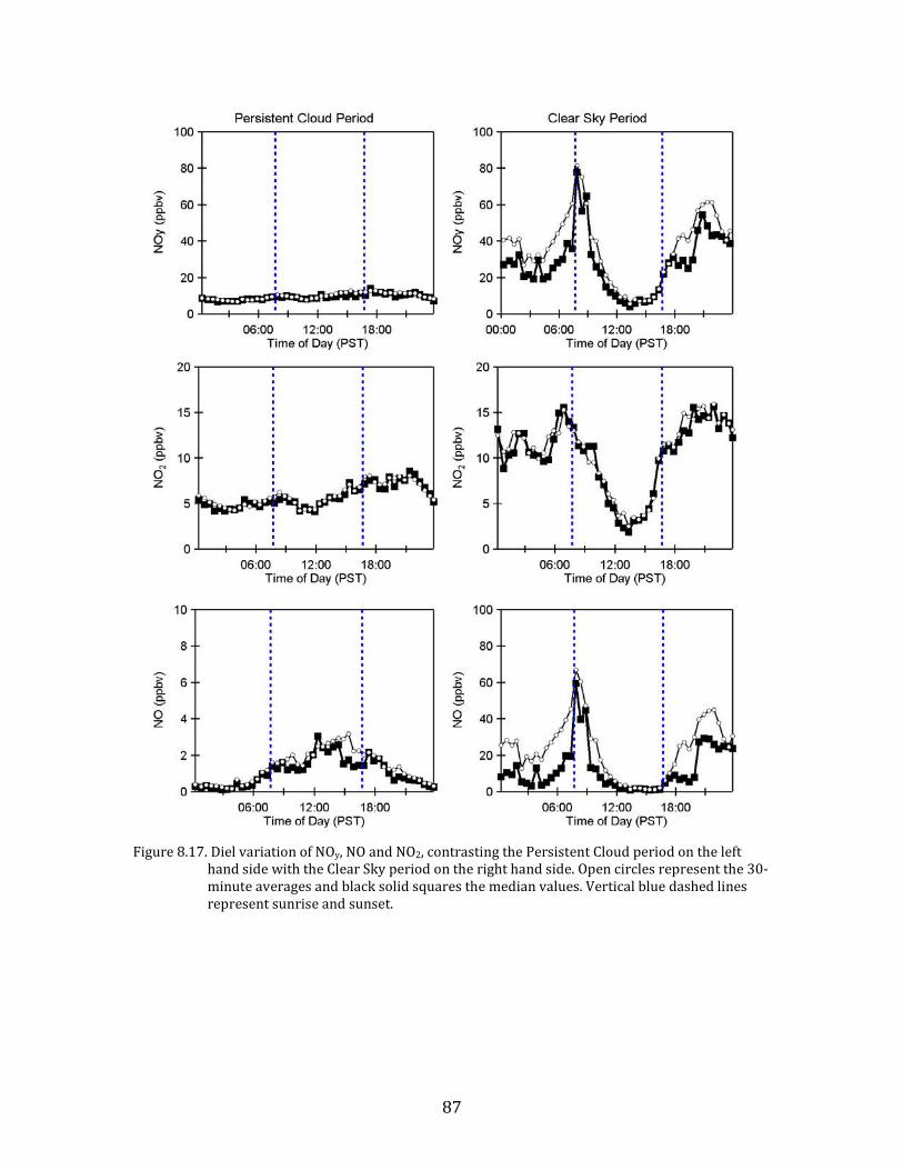
87
Figure 8.17. Diel variation of NOy, NO and NO2, contrasting the Persistent Cloud period on the left
hand side with the Clear Sky period on the right hand side. Open circles represent the 30-minute averages and black solid squares the median values. Vertical blue dashed lines represent sunrise and sunset.
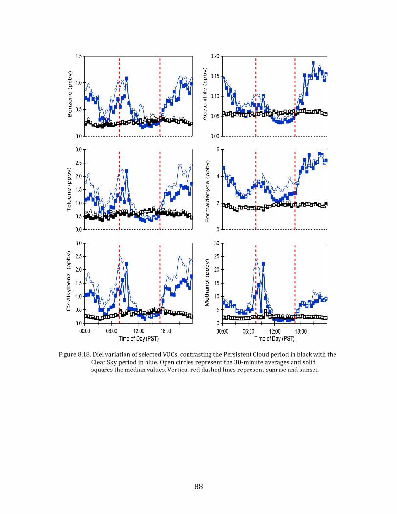
88
Figure 8.18. Diel variation of selected VOCs, contrasting the Persistent Cloud period in black with the
Clear Sky period in blue. Open circles represent the 30-minute averages and solid squares the median values. Vertical red dashed lines represent sunrise and sunset.
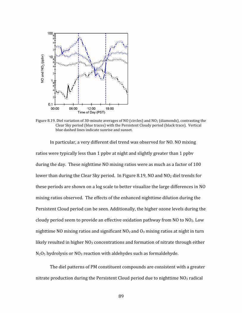
89
Figure 8.19. Diel variation of 30-minute averages of NO (circles) and NO2 (diamonds), contrasting the
Clear Sky period (blue traces) with the Persistent Cloudy period (black trace). Vertical blue dashed lines indicate sunrise and sunset.
In particular, a very different diel trend was observed for NO. NO mixing
ratios were typically less than 1 ppbv at night and slightly greater than 1 ppbv
during the day. These nighttime NO mixing ratios were as much as a factor of 100
lower than during the Clear Sky period. In Figure 8.19, NO and NO2 diel trends for
these periods are shown on a log scale to better visualize the large differences in NO
mixing ratios observed. The effects of the enhanced nighttime dilution during the
Persistent Cloud period can be seen. Additionally, the higher ozone levels during the
cloudy period seem to provide an effective oxidation pathway from NO to NO2. Low
nighttime NO mixing ratios and significant NO2 and O3 mixing ratios at night in turn
likely resulted in higher NO3 concentrations and formation of nitrate through either
N2O5 hydrolysis or NO3 reaction with aldehydes such as formaldehyde.
The diel patterns of PM constituent compounds are consistent with a greater
nitrate production during the Persistent Cloud period due to nighttime NO3 radical
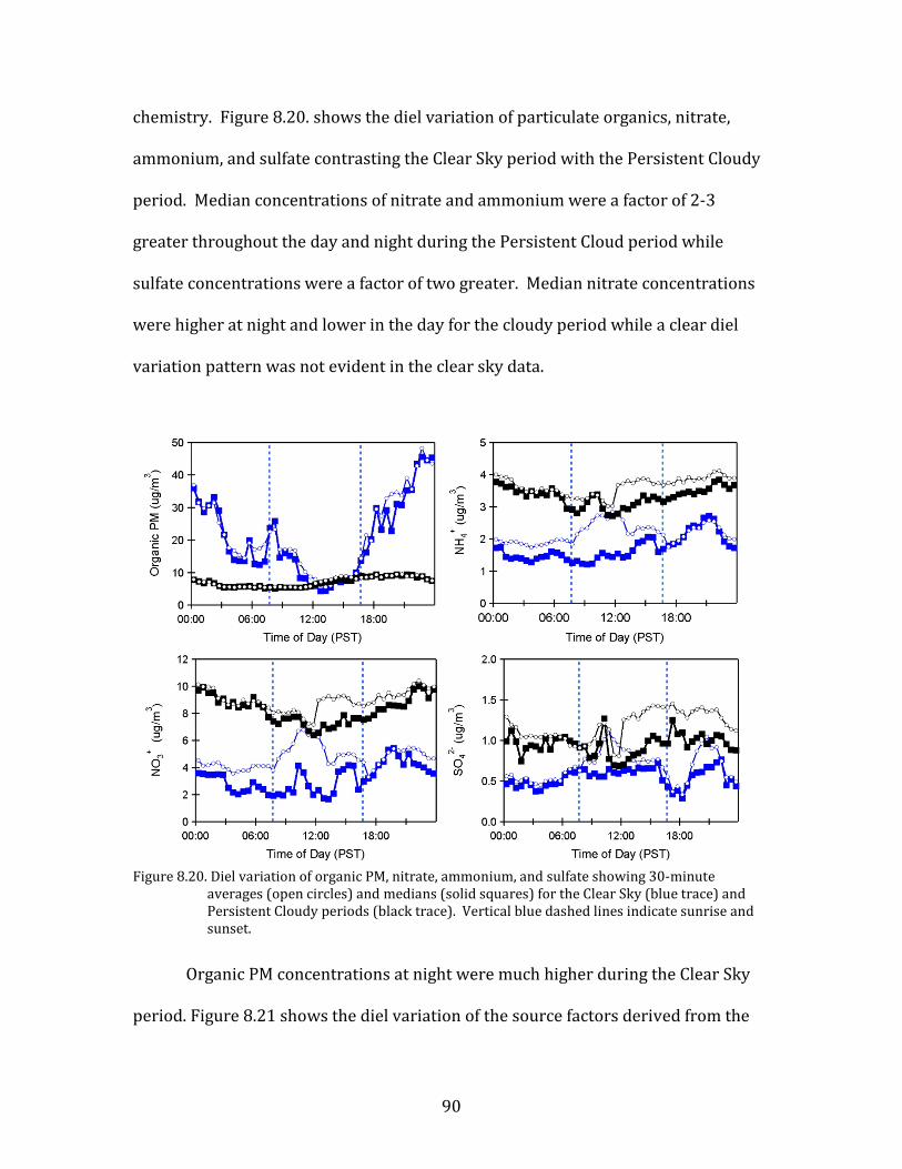
90
chemistry. Figure 8.20. shows the diel variation of particulate organics, nitrate,
ammonium, and sulfate contrasting the Clear Sky period with the Persistent Cloudy
period. Median concentrations of nitrate and ammonium were a factor of 2-3
greater throughout the day and night during the Persistent Cloud period while
sulfate concentrations were a factor of two greater. Median nitrate concentrations
were higher at night and lower in the day for the cloudy period while a clear diel
variation pattern was not evident in the clear sky data.
Figure 8.20. Diel variation of organic PM, nitrate, ammonium, and sulfate showing 30-minute
averages (open circles) and medians (solid squares) for the Clear Sky (blue trace) and Persistent Cloudy periods (black trace). Vertical blue dashed lines indicate sunrise and sunset.
Organic PM concentrations at night were much higher during the Clear Sky
period. Figure 8.21 shows the diel variation of the source factors derived from the
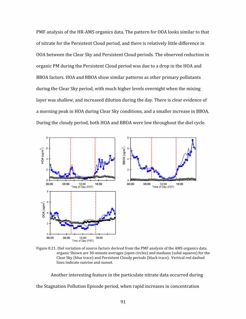
91
PMF analysis of the HR-AMS organics data. The pattern for OOA looks similar to that
of nitrate for the Persistent Cloud period, and there is relatively little difference in
OOA between the Clear Sky and Persistent Cloud periods. The observed reduction in
organic PM during the Persistent Cloud period was due to a drop in the HOA and
BBOA factors. HOA and BBOA show similar patterns as other primary pollutants
during the Clear Sky period, with much higher levels overnight when the mixing
layer was shallow, and increased dilution during the day. There is clear evidence of
a morning peak in HOA during Clear Sky conditions, and a smaller increase in BBOA.
During the cloudy period, both HOA and BBOA were low throughout the diel cycle.
Figure 8.21. Diel variation of source factors derived from the PMF analysis of the AMS organics data.
organic Shown are 30-minute averages (open circles) and medians (solid squares) for the Clear Sky (blue trace) and Persistent Cloudy periods (black trace). Vertical red dashed lines indicate sunrise and sunset.
Another interesting feature in the particulate nitrate data occurred during
the Stagnation Pollution Episode period, when rapid increases in concentration
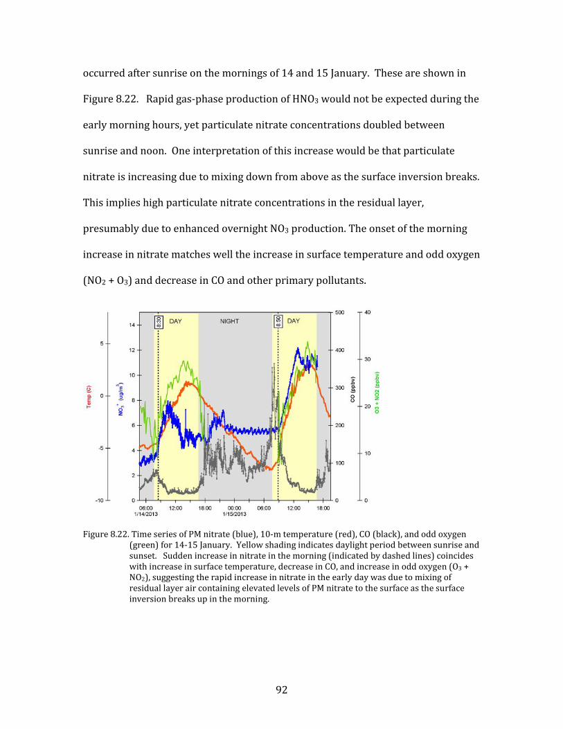
92
occurred after sunrise on the mornings of 14 and 15 January. These are shown in
Figure 8.22. Rapid gas-phase production of HNO3 would not be expected during the
early morning hours, yet particulate nitrate concentrations doubled between
sunrise and noon. One interpretation of this increase would be that particulate
nitrate is increasing due to mixing down from above as the surface inversion breaks.
This implies high particulate nitrate concentrations in the residual layer,
presumably due to enhanced overnight NO3 production. The onset of the morning
increase in nitrate matches well the increase in surface temperature and odd oxygen
(NO2 + O3) and decrease in CO and other primary pollutants.
Figure 8.22. Time series of PM nitrate (blue), 10-m temperature (red), CO (black), and odd oxygen
(green) for 14-15 January. Yellow shading indicates daylight period between sunrise and sunset. Sudden increase in nitrate in the morning (indicated by dashed lines) coincides with increase in surface temperature, decrease in CO, and increase in odd oxygen (O3 + NO2), suggesting the rapid increase in nitrate in the early day was due to mixing of residual layer air containing elevated levels of PM nitrate to the surface as the surface inversion breaks up in the morning.
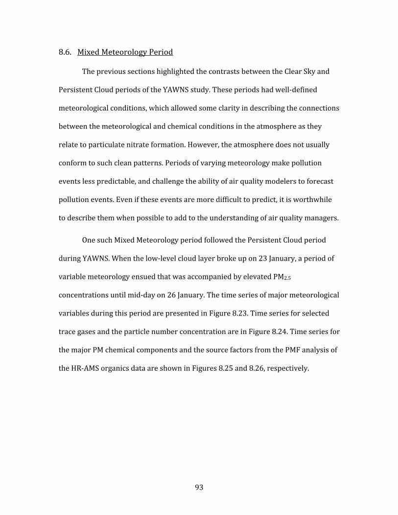
93
8.6. Mixed Meteorology Period
The previous sections highlighted the contrasts between the Clear Sky and
Persistent Cloud periods of the YAWNS study. These periods had well-defined
meteorological conditions, which allowed some clarity in describing the connections
between the meteorological and chemical conditions in the atmosphere as they
relate to particulate nitrate formation. However, the atmosphere does not usually
conform to such clean patterns. Periods of varying meteorology make pollution
events less predictable, and challenge the ability of air quality modelers to forecast
pollution events. Even if these events are more difficult to predict, it is worthwhile
to describe them when possible to add to the understanding of air quality managers.
One such Mixed Meteorology period followed the Persistent Cloud period
during YAWNS. When the low-level cloud layer broke up on 23 January, a period of
variable meteorology ensued that was accompanied by elevated PM2.5
concentrations until mid-day on 26 January. The time series of major meteorological
variables during this period are presented in Figure 8.23. Time series for selected
trace gases and the particle number concentration are in Figure 8.24. Time series for
the major PM chemical components and the source factors from the PMF analysis of
the HR-AMS organics data are shown in Figures 8.25 and 8.26, respectively.
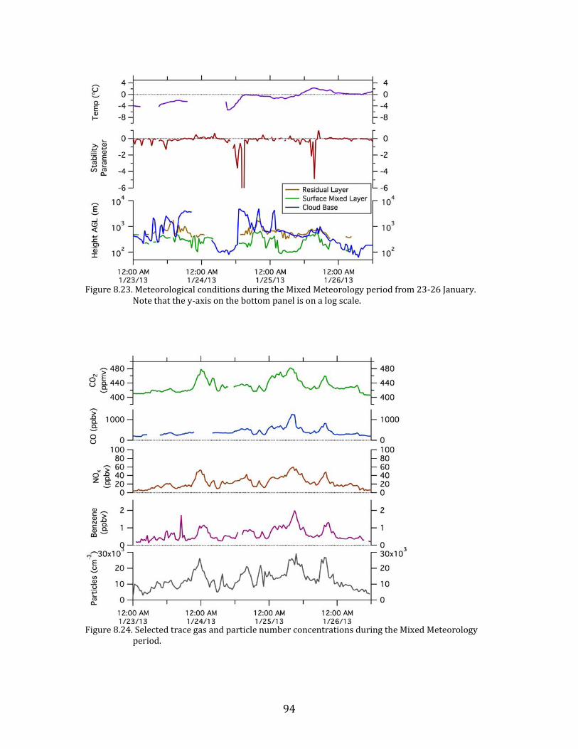
94
Figure 8.23. Meteorological conditions during the Mixed Meteorology period from 23-26 January.
Note that the y-axis on the bottom panel is on a log scale.
Figure 8.24. Selected trace gas and particle number concentrations during the Mixed Meteorology
period.
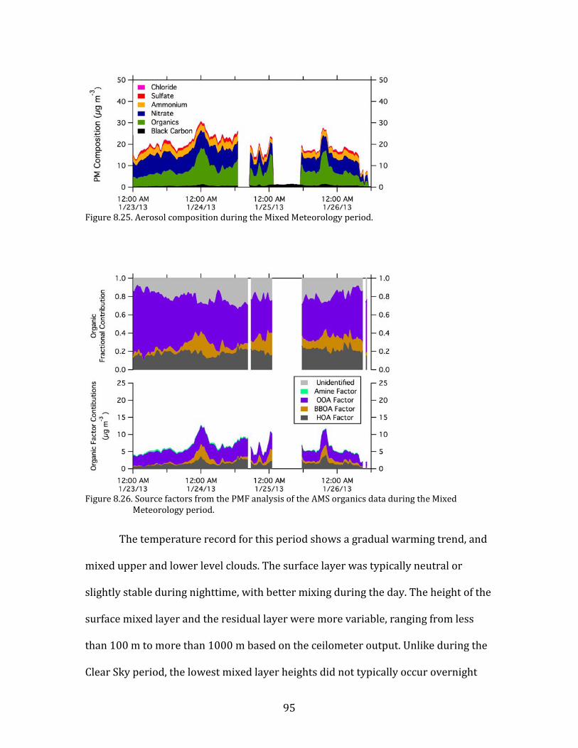
95
Figure 8.25. Aerosol composition during the Mixed Meteorology period.
Figure 8.26. Source factors from the PMF analysis of the AMS organics data during the Mixed
Meteorology period.
The temperature record for this period shows a gradual warming trend, and
mixed upper and lower level clouds. The surface layer was typically neutral or
slightly stable during nighttime, with better mixing during the day. The height of the
surface mixed layer and the residual layer were more variable, ranging from less
than 100 m to more than 1000 m based on the ceilometer output. Unlike during the
Clear Sky period, the lowest mixed layer heights did not typically occur overnight
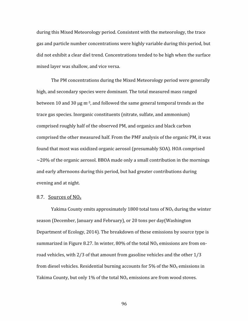
96
during this Mixed Meteorology period. Consistent with the meteorology, the trace
gas and particle number concentrations were highly variable during this period, but
did not exhibit a clear diel trend. Concentrations tended to be high when the surface
mixed layer was shallow, and vice versa.
The PM concentrations during the Mixed Meteorology period were generally
high, and secondary species were dominant. The total measured mass ranged
between 10 and 30 μg m-3, and followed the same general temporal trends as the
trace gas species. Inorganic constituents (nitrate, sulfate, and ammonium)
comprised roughly half of the observed PM, and organics and black carbon
comprised the other measured half. From the PMF analysis of the organic PM, it was
found that most was oxidized organic aerosol (presumably SOA). HOA comprised
~20% of the organic aerosol. BBOA made only a small contribution in the mornings
and early afternoons during this period, but had greater contributions during
evening and at night.
8.7. Sources of NOx
Yakima County emits approximately 1800 total tons of NOx during the winter
season (December, January and February), or 20 tons per day(Washington
Department of Ecology, 2014). The breakdown of these emissions by source type is
summarized in Figure 8.27. In winter, 80% of the total NOx emissions are from on-
road vehicles, with 2/3 of that amount from gasoline vehicles and the other 1/3
from diesel vehicles. Residential burning accounts for 5% of the NOx emissions in
Yakima County, but only 1% of the total NOx emissions are from wood stoves.
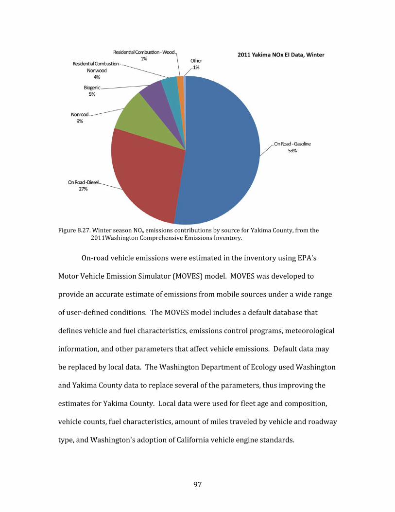
97
Figure 8.27. Winter season NOx emissions contributions by source for Yakima County, from the
2011Washington Comprehensive Emissions Inventory.
On-road vehicle emissions were estimated in the inventory using EPA's
Motor Vehicle Emission Simulator (MOVES) model. MOVES was developed to
provide an accurate estimate of emissions from mobile sources under a wide range
of user-defined conditions. The MOVES model includes a default database that
defines vehicle and fuel characteristics, emissions control programs, meteorological
information, and other parameters that affect vehicle emissions. Default data may
be replaced by local data. The Washington Department of Ecology used Washington
and Yakima County data to replace several of the parameters, thus improving the
estimates for Yakima County. Local data were used for fleet age and composition,
vehicle counts, fuel characteristics, amount of miles traveled by vehicle and roadway
type, and Washington's adoption of California vehicle engine standards.
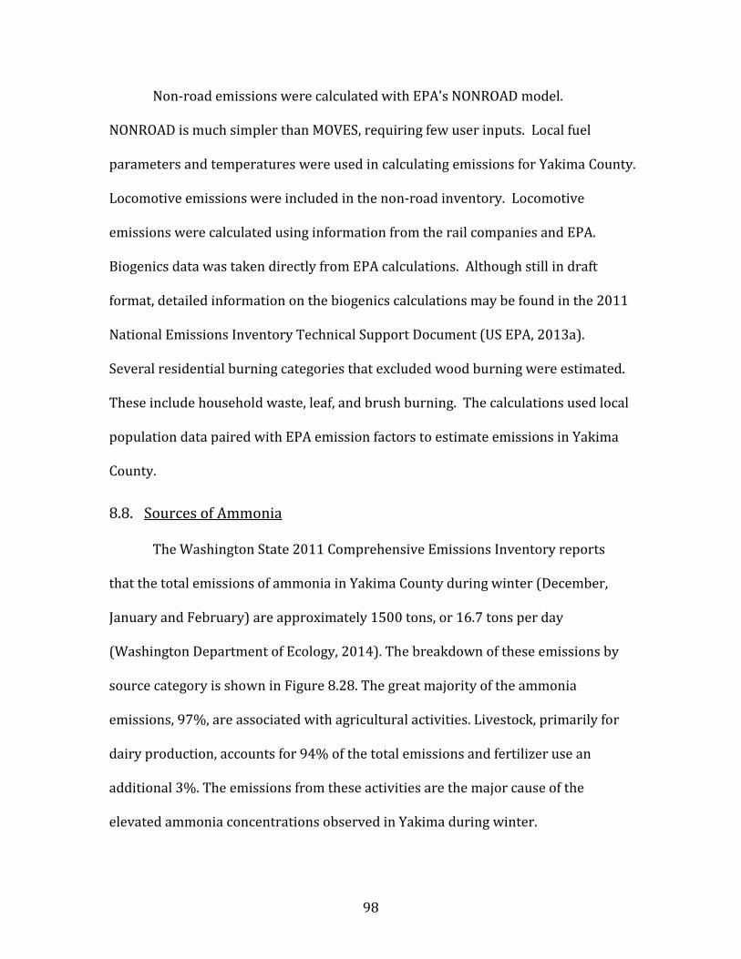
98
Non-road emissions were calculated with EPA's NONROAD model.
NONROAD is much simpler than MOVES, requiring few user inputs. Local fuel
parameters and temperatures were used in calculating emissions for Yakima County.
Locomotive emissions were included in the non-road inventory. Locomotive
emissions were calculated using information from the rail companies and EPA.
Biogenics data was taken directly from EPA calculations. Although still in draft
format, detailed information on the biogenics calculations may be found in the 2011
National Emissions Inventory Technical Support Document (US EPA, 2013a).
Several residential burning categories that excluded wood burning were estimated.
These include household waste, leaf, and brush burning. The calculations used local
population data paired with EPA emission factors to estimate emissions in Yakima
County.
8.8. Sources of Ammonia
The Washington State 2011 Comprehensive Emissions Inventory reports
that the total emissions of ammonia in Yakima County during winter (December,
January and February) are approximately 1500 tons, or 16.7 tons per day
(Washington Department of Ecology, 2014). The breakdown of these emissions by
source category is shown in Figure 8.28. The great majority of the ammonia
emissions, 97%, are associated with agricultural activities. Livestock, primarily for
dairy production, accounts for 94% of the total emissions and fertilizer use an
additional 3%. The emissions from these activities are the major cause of the
elevated ammonia concentrations observed in Yakima during winter.
99
Figure 8.28. Winter season NH3 emissions contributions by source for Yakima County, from the
2011Washington Comprehensive Emissions Inventory.
In the emissions inventory, local cattle population data from the Washington
State Department of Agriculture (WSDA) and US Department of Agriculture (USDA)
were used with emission factors from the Carnegie Mellon University (CMU)
Ammonia Model v.3.6 to estimate emissions from dairy and beef cattle (Pinder et al.,
2004). An EPA seasonal profile used in their Clean Air Interstate Rule modeling
platform was used to allocate emissions to each season: 13% of emissions to winter,
33% spring, 27% summer, and 28% fall. Other livestock emissions were taken from
version 1 of EPA's 2011 National Emissions Inventory (US EPA, 2013a). Fertilizer
emissions were calculated using WSDA's annual fertilizer tonnage report and
emission factors from the CMU Ammonia Model v.3.6. It is noted that a study done
by WSU at the Knott Dairy farm at WSU measured ammonia under different
100
meteorological conditions (Rumburg et al., 2005). Temperature, precipitation, and
wind speed influenced observed emissions. Generally, emissions were higher than
those calculated with the CMU model.
The possibility of additional ammonia contributions from leakage from large-
scale industrial chillers in Yakima was also investigated. Large amounts of ammonia
are typically stored onsite at chilling facilities for use as a refrigerant. To evaluate
whether leakage from chiller operations could contribute significantly to ambient
ammonia concentrations in Yakima, the Emergency Planning and Community Right-
to-know Act (EPCRA) database was consulted to locate all of the large chiller
facilities in Yakima. Fifty-four such facilities were found with Yakima addresses.
Since particulate ammonium nitrate is a secondary pollutant that forms over
relatively long time scales, the main question with respect to these chiller facilities
was whether they might cumulatively be contributing substantially to ambient NH3
concentrations in the Yakima area.
To investigate this, the US EPA AERSCREEN model (US EPA, 2013c) was used
to determine how possible leaks from a single facility would disperse downwind
under stagnant conditions. AERSCREEN produces worst case hourly concentrations
from a single source, by making very conservative assumptions about pollutant
dispersion. NH3 leakage was modeled as a non-buoyant (-30 °C) ground level point
source with negligible vertical velocity. Surrounding terrain was assumed to be flat
and located in an urban area.
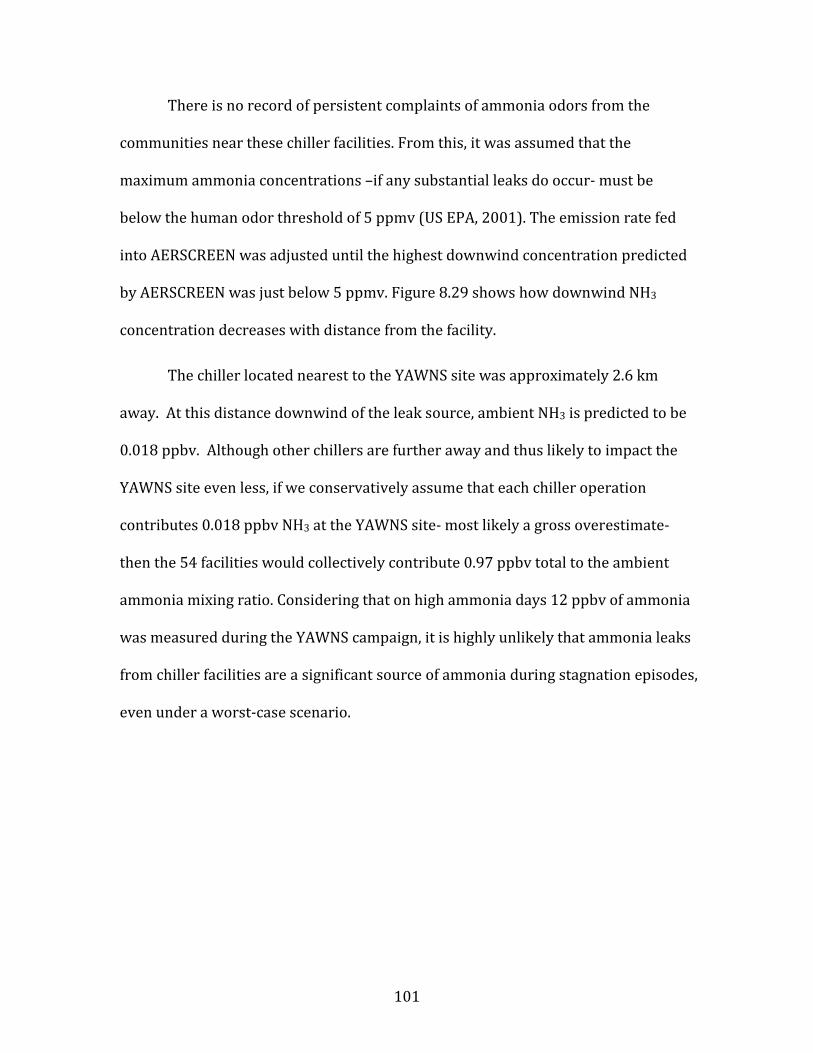
101
There is no record of persistent complaints of ammonia odors from the
communities near these chiller facilities. From this, it was assumed that the
maximum ammonia concentrations –if any substantial leaks do occur- must be
below the human odor threshold of 5 ppmv (US EPA, 2001). The emission rate fed
into AERSCREEN was adjusted until the highest downwind concentration predicted
by AERSCREEN was just below 5 ppmv. Figure 8.29 shows how downwind NH3
concentration decreases with distance from the facility.
The chiller located nearest to the YAWNS site was approximately 2.6 km
away. At this distance downwind of the leak source, ambient NH3 is predicted to be
0.018 ppbv. Although other chillers are further away and thus likely to impact the
YAWNS site even less, if we conservatively assume that each chiller operation
contributes 0.018 ppbv NH3 at the YAWNS site- most likely a gross overestimate-
then the 54 facilities would collectively contribute 0.97 ppbv total to the ambient
ammonia mixing ratio. Considering that on high ammonia days 12 ppbv of ammonia
was measured during the YAWNS campaign, it is highly unlikely that ammonia leaks
from chiller facilities are a significant source of ammonia during stagnation episodes,
even under a worst-case scenario.
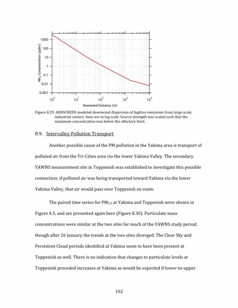
102
Figure 8.29. AERSCREEN modeled downwind dispersion of fugitive emissions from large-scale
industrial coolers. Axes are in log scale. Source strength was scaled such that the maximum concentration was below the olfactory limit.
8.9. Intervalley Pollution Transport
Another possible cause of the PM pollution in the Yakima area is transport of
polluted air from the Tri-Cities area via the lower Yakima Valley. The secondary
YAWNS measurement site in Toppenish was established to investigate this possible
connection; if polluted air was being transported toward Yakima via the lower
Yakima Valley, that air would pass over Toppenish en route.
The paired time series for PM2.5 at Yakima and Toppenish were shown in
Figure 4.5, and are presented again here (Figure 8.30). Particulate mass
concentrations were similar at the two sites for much of the YAWNS study period,
though after 26 January the trends at the two sites diverged. The Clear Sky and
Persistent Cloud periods identified at Yakima seem to have been present at
Toppenish as well. There is no indication that changes to particulate levels at
Toppenish preceded increases at Yakima as would be expected if lower-to-upper
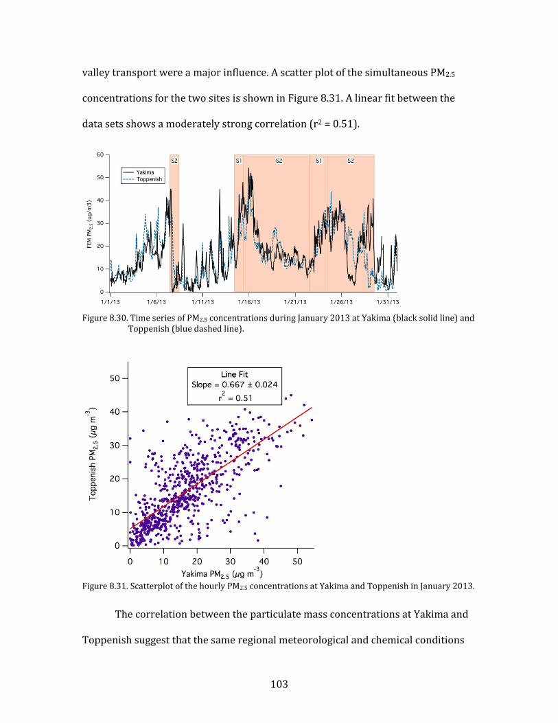
103
valley transport were a major influence. A scatter plot of the simultaneous PM2.5
concentrations for the two sites is shown in Figure 8.31. A linear fit between the
data sets shows a moderately strong correlation (r2 = 0.51).
Figure 8.30. Time series of PM2.5 concentrations during January 2013 at Yakima (black solid line) and
Toppenish (blue dashed line).
Figure 8.31. Scatterplot of the hourly PM2.5 concentrations at Yakima and Toppenish in January 2013.
The correlation between the particulate mass concentrations at Yakima and
Toppenish suggest that the same regional meteorological and chemical conditions
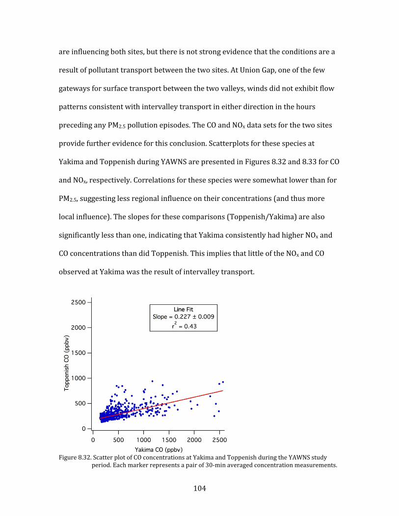
104
are influencing both sites, but there is not strong evidence that the conditions are a
result of pollutant transport between the two sites. At Union Gap, one of the few
gateways for surface transport between the two valleys, winds did not exhibit flow
patterns consistent with intervalley transport in either direction in the hours
preceding any PM2.5 pollution episodes. The CO and NOx data sets for the two sites
provide further evidence for this conclusion. Scatterplots for these species at
Yakima and Toppenish during YAWNS are presented in Figures 8.32 and 8.33 for CO
and NOx, respectively. Correlations for these species were somewhat lower than for
PM2.5, suggesting less regional influence on their concentrations (and thus more
local influence). The slopes for these comparisons (Toppenish/Yakima) are also
significantly less than one, indicating that Yakima consistently had higher NOx and
CO concentrations than did Toppenish. This implies that little of the NOx and CO
observed at Yakima was the result of intervalley transport.
Figure 8.32. Scatter plot of CO concentrations at Yakima and Toppenish during the YAWNS study
period. Each marker represents a pair of 30-min averaged concentration measurements.
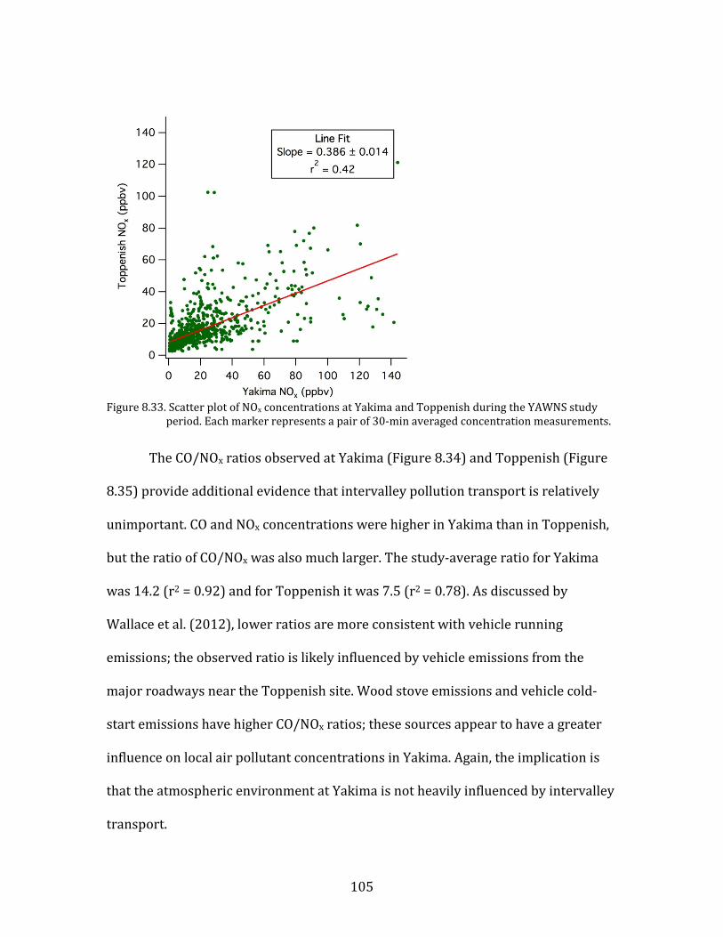
105
Figure 8.33. Scatter plot of NOx concentrations at Yakima and Toppenish during the YAWNS study
period. Each marker represents a pair of 30-min averaged concentration measurements.
The CO/NOx ratios observed at Yakima (Figure 8.34) and Toppenish (Figure
8.35) provide additional evidence that intervalley pollution transport is relatively
unimportant. CO and NOx concentrations were higher in Yakima than in Toppenish,
but the ratio of CO/NOx was also much larger. The study-average ratio for Yakima
was 14.2 (r2 = 0.92) and for Toppenish it was 7.5 (r2 = 0.78). As discussed by
Wallace et al. (2012), lower ratios are more consistent with vehicle running
emissions; the observed ratio is likely influenced by vehicle emissions from the
major roadways near the Toppenish site. Wood stove emissions and vehicle cold-
start emissions have higher CO/NOx ratios; these sources appear to have a greater
influence on local air pollutant concentrations in Yakima. Again, the implication is
that the atmospheric environment at Yakima is not heavily influenced by intervalley
transport.
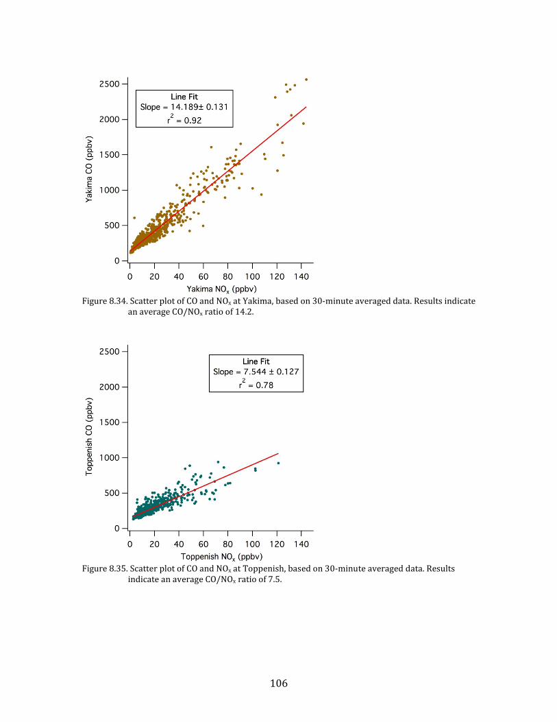
106
Figure 8.34. Scatter plot of CO and NOx at Yakima, based on 30-minute averaged data. Results indicate
an average CO/NOx ratio of 14.2.
Figure 8.35. Scatter plot of CO and NOx at Toppenish, based on 30-minute averaged data. Results
indicate an average CO/NOx ratio of 7.5.
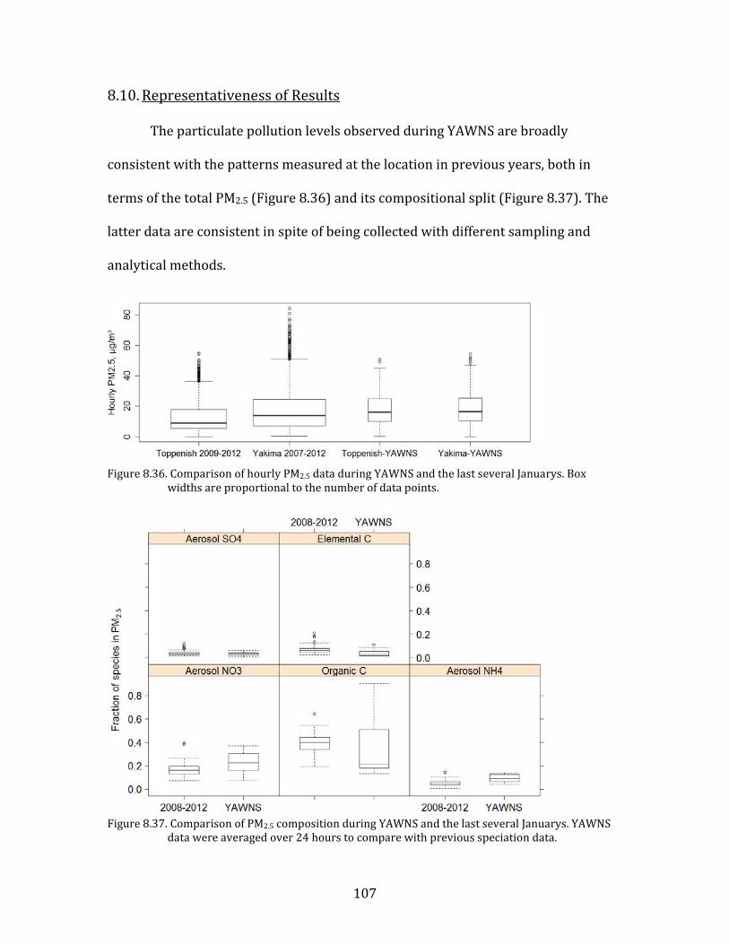
107
8.10. Representativeness of Results
The particulate pollution levels observed during YAWNS are broadly
consistent with the patterns measured at the location in previous years, both in
terms of the total PM2.5 (Figure 8.36) and its compositional split (Figure 8.37). The
latter data are consistent in spite of being collected with different sampling and
analytical methods.
Figure 8.36. Comparison of hourly PM2.5 data during YAWNS and the last several Januarys. Box
widths are proportional to the number of data points.
Figure 8.37. Comparison of PM2.5 composition during YAWNS and the last several Januarys. YAWNS
data were averaged over 24 hours to compare with previous speciation data.
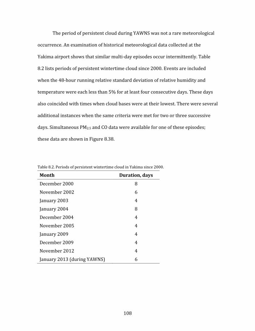
108
The period of persistent cloud during YAWNS was not a rare meteorological
occurrence. An examination of historical meteorological data collected at the
Yakima airport shows that similar multi-day episodes occur intermittently. Table
8.2 lists periods of persistent wintertime cloud since 2000. Events are included
when the 48-hour running relative standard deviation of relative humidity and
temperature were each less than 5% for at least four consecutive days. These days
also coincided with times when cloud bases were at their lowest. There were several
additional instances when the same criteria were met for two or three successive
days. Simultaneous PM2.5 and CO data were available for one of these episodes;
these data are shown in Figure 8.38.
Table 8.2. Periods of persistent wintertime cloud in Yakima since 2000.
Month Duration, days
December 2000 8
November 2002 6
January 2003 4
January 2004 8
December 2004 4
November 2005 4
January 2009 4
December 2009 4
November 2012 4
January 2013 (during YAWNS) 6
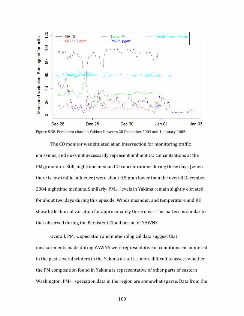
109
Figure 8.38. Persistent cloud in Yakima between 28 December 2004 and 1 January 2005.
The CO monitor was situated at an intersection for monitoring traffic
emissions, and does not necessarily represent ambient CO concentrations at the
PM2.5 monitor. Still, nighttime median CO concentrations during these days (when
there is low traffic influence) were about 0.5 ppm lower than the overall December
2004 nighttime medians. Similarly, PM2.5 levels in Yakima remain slightly elevated
for about two days during this episode. Winds meander, and temperature and RH
show little diurnal variation for approximately three days. This pattern is similar to
that observed during the Persistent Cloud period of YAWNS.
Overall, PM2.5, speciation and meteorological data suggest that
measurements made during YAWNS were representative of conditions encountered
in the past several winters in the Yakima area. It is more difficult to assess whether
the PM composition found in Yakima is representative of other parts of eastern
Washington. PM2.5 speciation data in the region are somewhat sparse. Data from the
110
IMPROVE network monitor at Wishram, Washington shows elevated particulate
nitrate fractions in wintertime PM2.5. IMPROVE data from White Pass, Snoqualmie
Pass, Pasayten, the Spokane Tribe, all in Washington, do not. Neither do historical
speciation data from Spokane, Washington and La Grande, Oregon. A recent source
apportionment study for urban areas in the Pacific Northwest (US EPA Region 10,
2013) highlights Boise and Salt Lake City as two other cities with significant
particulate nitrate concentrations during winter. These cities are larger, but are
located in valley topographies like Yakima; in each city nitrate comprises nearly
50% of the PM2.5 during wintertime pollution events, with organic material making
up much of the rest. Also like Yakima, Boise and Salt Lake City each have significant
sources of ammonia nearby. The parallels between these cities suggest that
comparative studies may be a fruitful approach for understanding how chemical and
meteorological processes interact to produce elevated PM levels in each region.
111
9. Summary and Future Plans
Episodes of elevated particulate nitrate in the Yakima Valley during winter
result from a combination of factors. The wintertime meteorology of the region
drives gas-particle equilibrium of ammonium nitrate strongly toward the particle
phase, and high relative humidity enhances this effect. High ammonia emissions
from agricultural sources in the area lead to elevated atmospheric concentrations of
the pollutant. This excess ammonia drives virtually all available nitric acid into the
particulate phase, forming particulate nitrate, and leads to a condition where any
additional nitric acid production would lead directly to greater particulate nitrate
levels. The production of particulate nitrate precursors is complicated and sensitive
to the varying meteorological and chemical conditions in the valley. Given the
backdrop of excess gaseous ammonia, there is usually sufficient reactive nitrogen in
the valley to produce elevated levels of particulate nitrate if the right meteorological
conditions take hold.
Two distinct meteorology conditions were observed where nitrate levels
were elevated. Under clear sky conditions, rapid increases of particulate nitrate in
the morning after sunrise on 14 and 15 January suggest that particulate nitrate had
formed in the residual layer and was being mixed down to the surface. During the
period where a persistent cloud-capped boundary layer was present, particulate
nitrate remained moderately elevated through the day and night. In this case it
appears likely that surface emissions are mixed through the depth of the cloud-
capped boundary layer day and night, with the boundary layer height determined by
112
cloud top height. This condition facilitates particulate nitrate formation by keeping
nighttime NO mixing ratios low, which promotes formation of NO3 radical at
night. Particulate nitrate could then be formed either from the uptake of N2O5 and
subsequent hydrolysis onto existing particles or from partitioning of gas-phase
nitric acid produced from NO3 + aldehyde reactions. Given the measured
abundance of NH3 and cold temperatures, gas-phase HNO3 mixing ratios are
expected to be low and the formation of particulate nitrate is limited by the
availability of HNO3.
Little evidence was found that pollution in Yakima is significantly impacted
from regional transport via the Lower Yakima Valley. While meteorological
conditions and PM2.5 levels were typically similar at Yakima and Toppenish, the
levels of NOx and CO indicated clearly that Yakima air quality was dominated by
local sources. Additionally, it was found that the YAWNS study period was broadly
representative of the typical wintertime meteorology and air quality conditions at
Yakima. While not previously described in detail, persistent cloudy periods occur
occasionally and have a clear impact on local air quality. Furthermore, the air
quality in Yakima itself is consistent with other regional cities with a similar mix of
emissions sources. In general, when elevated ammonia concentrations from
agriculture mix with urban NOx emissions in winter, elevated particulate nitrate is
common.
113
9.1. Air Quality Management Implications
• Ammonia emissions reductions are unlikely to result in significant
reductions in wintertime particulate nitrate unless order-of-magnitude
reductions are viable. As it stands, the ammonia levels in winter are high
enough that all available nitric acid is driven to particulate nitrate.
• The pathway to reducing the available nitric acid / particulate nitrate pool is
not obvious. Particulate nitrate is the major atmospheric endpoint for NOx, so
ultimately NOx reduction would reduce the potential particulate nitrate pool.
However, NO also inhibits the formation of particulate nitrate by destroying
the nitrate radical, which is an important intermediate species. Therefore it is
entirely possible that a local NOx reduction would skew the local atmospheric
chemistry toward more local particulate nitrate production. A numerical
modeling effort is required to determine the specific system behavior.
• During the persistent cloud conditions, mixing occurs throughout the cloud
layer and perhaps beyond, resulting in reduced levels of some pollutants,
including primary PM. While a reduction in the relative contribution wood
smoke to organic PM is apparent during burn bans, calling or continuing
burn bans during persistent cloud conditions might be less critical than
during clear sky stagnation events. However, in addition to reducing
exposure to the direct wood smoke emissions, burn bans may also reduce
exposure to secondary organic aerosol. SOA in Yakima is thought to originate,
in part, from the processing of wood smoke PM throughout the mixed layer.
114
• The cloud-capped condition is linked to elevated secondary PM levels. Thus
the onset of cloud shifts the type of PM present, but elevated concentrations
would still be expected to be associated with the meteorological condition.
• During YAWNS, burn bans appear to have been called at the correct times in
Yakima, especially during clear sky and mixed meteorological conditions. The
potential for elevated pollution was anticipated for the clear-sky stagnation
period. During mixed-meteorology periods, forecasting remains a challenge.
It may be possible to adjust responses to anticipate the likely increased
mixing associated with persistent low-level cloud. While meteorological
models do not reliably predict such cloudy periods, once they set in they are
clearly identifiable. It may be possible to relax policy responses more
confidently when persistent cloud is accompanied by slight reductions in the
observed PM2.5 levels.
9.2. Recommendations for Additional Study
• One key question arising from this work is the frequency of persistent cloud
episodes in the valleys of Washington State, and whether this meteorological
condition consistently results in enhanced dilution of primary pollutants. The
meteorological question could be explored using a data mining approach
with the extensive meteorological sensor networks available in the state. The
air quality link is more challenging; to study this would likely require the
deployment of a network of reliable low-cost sensors for a representative
primary pollutant such as CO.
115
• The chemical processing within the Yakima Valley that leads to enhanced
particulate nitrate formation under certain conditions remains unclear and
should be explored further. The vertical profiles of key species for both
daytime and nighttime, and clear and cloudy conditions is key. This effort
could be initiated using a 1-D vertical chemical model where the appropriate
meteorology is proscribed. The study would be greatly enhanced by the
availability of additional surface and vertical profile measurements of the key
chemical species, including HNO3 and N2O5.
• The YAWNS data set provides an invaluable basis for evaluating the
AIRPACT-4 modeling framework under wintertime conditions. It is
anticipated that air quality predictability will prove poor during the
Persistent Cloud period due to inadequate performance of WRF, the
underlying meteorological model. The model performance test would be
more appropriate during other portions of the study. An AIRPACT-4 study
could also examine the potential effectiveness of various particulate nitrate
reduction strategies. The sensitivity of particulate nitrate levels to ammonia
versus NOx control could be evaluated in this manner.
• Effectively forecasting air quality during clear sky stagnation and low-level
cloud conditions requires accurate modeling of the surface mixing layer.
WRF at a 4-km resolution is currently unable to adequately represent
persistent cold air pools, making reliable air quality forecasts challenging.
There are ongoing research studies in the intermountain west to better
understand the meteorology of persistent cold air pools. Progress would be

116
significantly enhanced if the parallel meteorology and air quality research
efforts could be merged.
117
10. References
Aiken, A. C., de Foy, B., Wiedinmyer, C., DeCarlo, P. F., Ulbrich, I. M., Wehrli, M. N., Szidat, S., Prevot, A. S. H., Noda, J., Wacker, L., Volkamer, R., et al.: Mexico city aerosol analysis during MILAGRO using high resolution aerosol mass spectrometry at the urban supersite (T0) – Part 2: Analysis of the biomass burning contribution and the non-fossil carbon fraction, Atmos Chem Phys, 10(12), 5315–5341, doi:10.5194/acp-10-5315-2010, 2010.
Aiken, A. C., Salcedo, D., Cubison, M. J., Huffman, J. A., DeCarlo, P. F., Ulbrich, I. M., Docherty, K. S., Sueper, D., Kimmel, J. R., Worsnop, D. R., Trimborn, A., et al.: Mexico City aerosol analysis during MILAGRO using high resolution aerosol mass spectrometry at the urban supersite (T0) – Part 1: Fine particle composition and organic source apportionment, Atmos Chem Phys, 9(17), 6633–6653, doi:10.5194/acp-9-6633-2009, 2009.
Allan, J. D., Delia, A. E., Coe, H., Bower, K. N., Alfarra, M. R., Jimenez, J. L., Middlebrook, A. M., Drewnick, F., Onasch, T. B., Canagaratna, M. R., Jayne, J. T., et al.: A generalised method for the extraction of chemically resolved mass spectra from Aerodyne aerosol mass spectrometer data, J. Aerosol Sci., 35(7), 909–922, doi:10.1016/j.jaerosci.2004.02.007, 2004.
BC Air Quality: Venting Index, Venting Index [online] Available from: http://www.bcairquality.ca/readings/ventilation-index.html (Accessed 24 January 2014), 2014.
Campbell Scientific, Inc.: Instruction Manual: CSAT3 three-dimensional sonic anemometer, Logan, Utah, USA., 2006.
Chazette, P., Couvert, P., Randriamiarisoa, H., Sanak, J., Bonsang, B., Moral, P., Berthier, S., Salanave, S. and Toussaint, F.: Three-Dimensional Survey of Pollution During Winter in French Alps Valleys, Atmos. Environ., 39(6), 1035–1047, doi:10.1016/j.atmosenv.2004.10.014, 2005.
DeCarlo, P. F., Kimmel, J. R., Trimborn, A., Northway, M. J., Jayne, J. T., Aiken, A. C., Gonin, M., Fuhrer, K., Horvath, T., Docherty, K. S., Worsnop, D. R., et al.: Field-Deployable, High-Resolution, Time-of-Flight Aerosol Mass Spectrometer, Anal Chem, 78(24), 8281–8289, doi:10.1021/ac061249n, 2006.
Erickson, M. H., Gueneron, M. and Jobson, B. T.: Measuring long chain alkanes in diesel engine exhaust by thermal desorption PTR-MS, Atmospheric Meas. Tech., 7(1), 225–239, doi:10.5194/amt-7-225-2014, 2014.
Hildebrandt, L., Kostenidou, E., Lanz, V. A., Prevot, A. S. H., Baltensperger, U., Mihalopoulos, N., Laaksonen, A., Donahue, N. M. and Pandis, S. N.: Sources and
118
atmospheric processing of organic aerosol in the Mediterranean: insights from aerosol mass spectrometer factor analysis, Atmos Chem Phys, 11(23), 12499–12515, doi:10.5194/acp-11-12499-2011, 2011.
Jayne, J. T., Leard, D. C., Zhang, X., Davidovits, P., Smith, K. A., Kolb, C. E. and Worsnop, D. R.: Development of an Aerosol Mass Spectrometer for Size and Composition Analysis of Submicron Particles, Aerosol Sci. Technol., 33(1-2), 49–70, doi:10.1080/027868200410840, 2000.
Jimenez Group Wiki: ToF-AMS Main, [online] Available from: http://cires.colorado.edu/jimenez-group/wiki/index.php?title=ToF-AMS_Main, 2013.
Jobson, B. T. and McCoskey, J. K.: Sample drying to improve HCHO measurements by PTR-MS instruments: laboratory and field measurements, Atmospheric Chem. Phys., 10(4), 1821–1835, doi:10.5194/acp-10-1821-2010, 2010.
Kuhns, H., Bohdan, V., Chow, J., Etyemezian, V., Green, M., Herlocker, D., Kohl, S., McGown, M., Ramsdell, J., Stockwell, W., Toole, M., et al.: The Treasure Valley secondary aerosol study I: measurements and equilibrium modeling of inorganic secondary aerosols and precursors for southwestern Idaho, Atmos. Environ., 37(4), 511–524, 2003.
Laborde, M., Schnaiter, M., Linke, C., Saathoff, H., Naumann, K.-H., Moehler, O., Berlenz, S., Wagner, U., Taylor, J. W., Liu, D., Flynn, M., et al.: Single Particle Soot Photometer intercomparison at the AIDA chamber, Atmospheric Meas. Tech., 5(12), 3077–3097, doi:10.5194/amt-5-3077-2012, 2012.
Lim, S. S., Vos, T., Flaxman, A. D., Danaei, G., Shibuya, K., Adair-Rohani, H., AlMazroa, M. A., Amann, M., Anderson, H. R., Andrews, K. G., Aryee, M., et al.: A comparative risk assessment of burden of disease and injury attributable to 67 risk factors and risk factor clusters in 21 regions, 1990–2010: a systematic analysis for the Global Burden of Disease Study 2010, The Lancet, 380(9859), 2224–2260, doi:10.1016/S0140-6736(12)61766-8, 2012.
Lindinger, W., Hansel, A. and A. Jordan: On-line monitoring of volatile organic compounds at pptv levels by means of Proton-Transfer-Reaction Mass Spectrometry (PTR-MS) Medical applications, food control and environmental research, Int. J. Mass Spectrom., 173, 191–241, 1998.
Mwaniki, G. R., Rosenkrance, C., Wallace, H. W., Jobson, B. T., Erickson, M. H., Lamb, B. K., Zalakeviciute, R. and VanReken, T. M.: Factors Contributing to Elevated Concentrations of PM2.5 during Wintertime near Boise, Idaho, Atmospheric Pollut. Res., in press, 2014.
NOAA NOWData: Yakima Area climatic data, [online] Available from: http://www.nws.noaa.gov/climate/xmacis.php?wfo=pdt, 2013.
119
Pinder, R. W., Strader, R., Davidson, C. I. and Adams, P. J.: A temporally and spatially resolved ammonia emission inventory for dairy cows in the United States, Atmos. Environ., 38(23), 3747–3756, doi:10.1016/j.atmosenv.2004.04.008, 2004.
Pope, C., Burnett, R., Thun, M., Calle, E., Krewski, D., Ito, K. and Thurston, G.: Lung Cancer, Cardiopulmonary Mortality, and Long-Term Exposure to Fine Particulate Air Pollution, J Amer Med Assoc, 287(9), 1132–1141, 2002.
RCW, 70.94.473: Limitations on burning wood for heat — First and second stage burn bans — Report on second stage burn ban., Revis. Code Wash., n.d.
Rumburg, B., Chen, J., Mount, G. and Lamb, B.: Washington State Dairy Ammonia emissions Model - Final Report, Washington State University, Laboratory for Atmospheric Research, Department of Civil & Environmental Engineering, Pullman, Washington., 2005.
Schwarz, J. P., Gao, R. S., Fahey, D. W., Thomson, D. S., Watts, L. A., Wilson, J. C., Reeves, J. M., Darbeheshti, M., Baumgardner, D. G., Kok, G. L., Chung, S. H., et al.: Single-particle measurements of midlatitude black carbon and light-scattering aerosols from the boundary layer to the lower stratosphere, J. Geophys. Res.-Atmospheres, 111(D16), doi:10.1029/2006JD007076, 2006.
Seinfeld, J. H. and Pandis, S. N.: Atmospheric Chemistry and Physics: From Air Pollution to Climate Change, 2nd ed., Wiley-Interscience., 2006.
Silva, P., Vawdrey, E., Corbett, M. and Erupe, M.: Fine particle concentrations and composition during wintertime inversions in Logan, Utah, USA, Atmos. Environ., 41(26), 5410–5422, doi:10.1016/j.atmosenv.2007.02.016, 2007.
Stockwell, W., Kuhns, H., Etyemezian, V., Green, M., Chow, J. and Watson, J.: The Treasure Valley secondary aerosol study II: modeling of the formation of inorganic secondary aerosols and precursors for southwestern Idaho, Atmos. Environ., 37(4), 525–534, doi:10.1016/S1352-2310(02)00895-6, 2003.
Ulbrich, I. M., Canagaratna, M. R., Zhang, Q., Worsnop, D. R. and Jimenez, J. L.: Interpretation of organic components from Positive Matrix Factorization of aerosol mass spectrometric data, Atmos Chem Phys, 9(9), 2891–2918, doi:10.5194/acp-9-2891-2009, 2009.
US EPA: Hazards of Ammonia Releases at Ammonia Refrigeration Facilities (Update). [online] Available from: http://www.epa.gov/oem/docs/chem/ammonia.pdf (Accessed 8 February 2014), 2001.
US EPA: 2011 National Emissions Inventory, version 1: Technical Support Document, Draft. [online] Available from: http://www.epa.gov/ttn/chief/net/2011nei/2011_neiv1_tsd_draft.pdf, 2013a.
120
US EPA: National Ambient Air Quality Standards (NAAQS), [online] Available from: http://www.epa.gov/air/criteria.html (Accessed 19 December 2013b), 2013.
US EPA: Screening Models | TTN - Support Center for Regulatory Atmospheric Modeling | US EPA, [online] Available from: http://www.epa.gov/scram001/dispersion_screening.htm (Accessed 27 January 2014c), 2013.
US EPA Region 10: Source apportionment modeling for multiple urban PM2.5 chemical speciation sites within the Pacific Northwest., 2013.
Vaisala, Inc.: User’s guide: Vaisala boundary layer view software BL-VIEW., 2010.
Wallace, H. W., Jobson, B. T., Erickson, M. H., McCoskey, J. K., VanReken, T. M., Lamb, B. K., Vaughan, J. K., Hardy, R. J., Cole, J. L., Strachan, S. M. and Zhang, W.: Comparison of wintertime CO to NOx ratios to MOVES and MOBILE6.2 on-road emissions inventories, Atmos Env., 63, 289–297, doi:10.1016/j.atmosenv.2012.08.062, 2012.
Washington Department of Ecology: An Evaluation of Two-Stage Burn Bans in Washington: Report to the Legislature. [online] Available from: https://fortress.wa.gov/ecy/publications/publications/1102021.pdf, 2011.
Washington Department of Ecology: Washington State 2011 Comprehensive Emissions Inventory, Air Quality Program, Washington State Department of Ecology. Draft Report and datasets., 2014.
Webb, E. K., Pearman, G. I. and Leuning, R.: Correction of flux measurements for density effects due to heat and water-vapor transfer, Q. J. R. Meteorol. Soc., 106(447), 85–100, 1980.
Wood, R.: Stratocumulus Clouds, Mon. Weather Rev., 140(8), 2373–2423, doi:10.1175/MWR-D-11-00121.1, 2012.
Zhang, Q., Jimenez, J. L., Canagaratna, M. R., Ulbrich, I. M., Ng, N. L., Worsnop, D. R. and Sun, Y.: Understanding atmospheric organic aerosols via factor analysis of aerosol mass spectrometry: a review, Anal. Bioanal. Chem., doi:10.1007/s00216-011-5355-y [online] Available from: http://www.springerlink.com/content/p5h2278x11m42682/ (Accessed 17 October 2011), 2011.
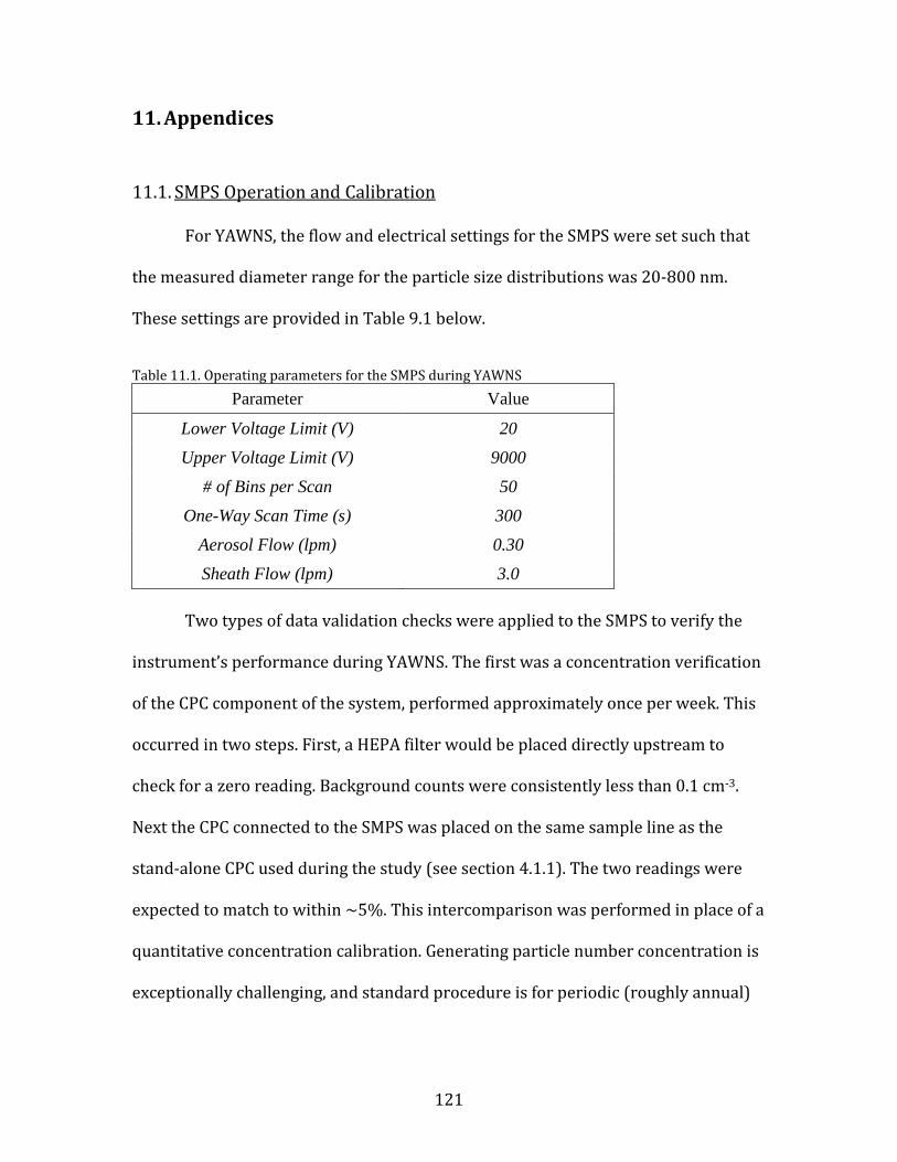
121
11. Appendices
11.1. SMPS Operation and Calibration
For YAWNS, the flow and electrical settings for the SMPS were set such that
the measured diameter range for the particle size distributions was 20-800 nm.
These settings are provided in Table 9.1 below.
Table 11.1. Operating parameters for the SMPS during YAWNS Parameter Value
Lower Voltage Limit (V) 20 Upper Voltage Limit (V) 9000
# of Bins per Scan 50 One-Way Scan Time (s) 300
Aerosol Flow (lpm) 0.30 Sheath Flow (lpm) 3.0
Two types of data validation checks were applied to the SMPS to verify the
instrument’s performance during YAWNS. The first was a concentration verification
of the CPC component of the system, performed approximately once per week. This
occurred in two steps. First, a HEPA filter would be placed directly upstream to
check for a zero reading. Background counts were consistently less than 0.1 cm-3.
Next the CPC connected to the SMPS was placed on the same sample line as the
stand-alone CPC used during the study (see section 4.1.1). The two readings were
expected to match to within ~5%. This intercomparison was performed in place of a
quantitative concentration calibration. Generating particle number concentration is
exceptionally challenging, and standard procedure is for periodic (roughly annual)
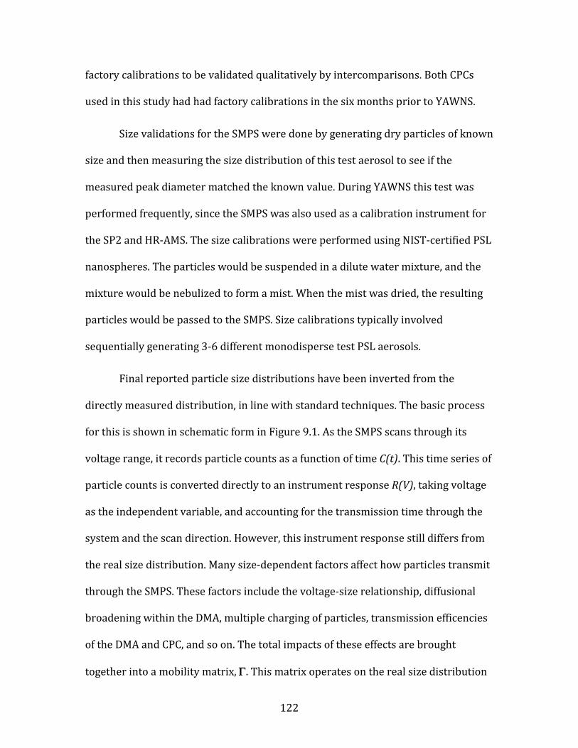
122
factory calibrations to be validated qualitatively by intercomparisons. Both CPCs
used in this study had had factory calibrations in the six months prior to YAWNS.
Size validations for the SMPS were done by generating dry particles of known
size and then measuring the size distribution of this test aerosol to see if the
measured peak diameter matched the known value. During YAWNS this test was
performed frequently, since the SMPS was also used as a calibration instrument for
the SP2 and HR-AMS. The size calibrations were performed using NIST-certified PSL
nanospheres. The particles would be suspended in a dilute water mixture, and the
mixture would be nebulized to form a mist. When the mist was dried, the resulting
particles would be passed to the SMPS. Size calibrations typically involved
sequentially generating 3-6 different monodisperse test PSL aerosols.
Final reported particle size distributions have been inverted from the
directly measured distribution, in line with standard techniques. The basic process
for this is shown in schematic form in Figure 9.1. As the SMPS scans through its
voltage range, it records particle counts as a function of time C(t). This time series of
particle counts is converted directly to an instrument response R(V), taking voltage
as the independent variable, and accounting for the transmission time through the
system and the scan direction. However, this instrument response still differs from
the real size distribution. Many size-dependent factors affect how particles transmit
through the SMPS. These factors include the voltage-size relationship, diffusional
broadening within the DMA, multiple charging of particles, transmission efficencies
of the DMA and CPC, and so on. The total impacts of these effects are brought
together into a mobility matrix, Γ. This matrix operates on the real size distribution
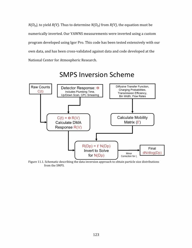
123
N(Dp), to yield R(V). Thus to determine N(Dp) from R(V), the equation must be
numerically inverted. Our YAWNS measurements were inverted using a custom
program developed using Igor Pro. This code has been tested extensively with our
own data, and has been cross-validated against data and code developed at the
National Center for Atmospheric Research.
Figure 11.1. Schematic describing the data inversion approach to obtain particle size distributions
from the SMPS.
124
11.2. HR-AMS Operation and Data Analysis
An Aerodyne high-resolution time-of-flight aerosol mass spectrometer (HR-
AMS) allows for the direct separation and measurement of most ions at the same
nominal m/z, quantification of organic and inorganic components, and the
determination of the size distribution of all ions. The HR-AMS uses automated data
analysis routines to classify the peaks in the mass spectrum into the following
species classes: organics, ammonium, sulfate, nitrate, and chlorides. Concentrations
for these species are given in near real-time. The instrument can operate under two
ion optical modes, referred to as V-mode and W-mode. V-mode is a single-reflection
configuration allowing for higher sensitivity at lower resolution, while W-mode is a
two-reflection configuration offering a lower sensitivity but higher resolution. A
schematic of HR-AMS found in Figure 11.2. Aerosol particles enter through a
sampling inlet that restricted flow with a 110 µm critical orifice at a flow rate of
approximately 1.5 cm3 s-1 and into an aerodynamic lens. The aerodynamic lens
focuses particles (ranging from 35 to 1500 nm) into a narrow beam using six
apertures of sequentially decreasing size. At this stage most of the atmospheric gas
surrounding the particles is removed.
After transmission through the aerodynamic lens, the focused aerosol beam
is accelerated in a supersonic expansion caused by the difference in pressure
between the sampling and sizing chambers. This acceleration results in different
velocities for aerosols of different sizes. The instrument is typically alternated
between two modes of operation that change how particle transmission through the
sizing chamber occurs; these are mass spectrum (MS) mode and particle time-of-
125
flight (PToF) mode. These modes are controlled by the positioning of a mechanical
chopper wheel, located directly after the particle beam exit from the aerodynamic
lens. In MS mode, particles travel unimpeded until they impact onto a resistively-
heated porous tungsten surface held at 600 °C. Here the volatile and semi-volatile
portions of the aerosols are vaporized and then immediately ionized using 70-eV
electron-impact ionization source. The mass spectrometer detects the positive ion
fragments generated by the electron impact ionization and determines the mass-to-
charge (m/z) distribution of the particle beam. When operating in PToF mode,
particle size can be determined by measuring flight times across a fixed distance.
The rotating chopper wheel consist of with two radial slits located 180° apart and
when rotating intercepts the focused particle beam. As the particles travel on a
straight path through the sizing chamber, they separate according to their size with
the smaller particles traveling faster than the larger particles. Particles are thus
classified by size in the sizing chamber and then also classified by their mass
spectrum, allowing time-averaged composition-resolved size distributions to be
obtained. The AMS detects non-refractory species which can evaporate rapidly at
the AMS temperature and vacuum conditions (mostly volatile and semi-volatile
components) sulfate, nitrate, ammonium, chloride, and total organic matter; while it
does not measure non-volatile constituents like crustal oxides, sea salt, and black
carbon. More detailed information on the HR-AMS can be found elsewhere (DeCarlo
et al., 2006).
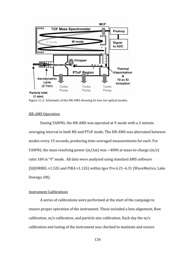
126
Figure 11.2. Schematic of the HR-AMS showing its two ion optical modes.
HR-AMS Operation
During YAWNS, the HR-AMS was operated at V-mode with a 2-minute
averaging interval in both MS and PToF mode. The HR-AMS was alternated between
modes every 15 seconds, producing time-averaged measurements for each. For
YAWNS, the mass resolving power (m/∆m) was ~4000 at mass-to-charge (m/z)
ratio 184 in “V” mode. All data were analyzed using standard AMS software
(SQUIRREL v1.52G and PIKA v1.12G) within Igor Pro 6.21–6.31 (WaveMetrics, Lake
Oswego, OR).
Instrument Calibrations
A series of calibrations were performed at the start of the campaign to
ensure proper operation of the instrument. These included a lens alignment, flow
calibration, m/z calibration, and particle size calibration. Each day the m/z
calibration and tuning of the instrument was checked to maintain and ensure
127
quality measurements throughout the campaign. An Ionization Efficiency (IE)
calibration was performed at the beginning, middle, and end of campaign. Table
11.2 details the major calibration activities for the HR-AMS during and YAWNS.
Table 11.2. Calibration activities for the HR-AMS during YAWNS.
Calibration Date Performed
Lens Alignment 01/06/13
m/z Calibration 01/06/13
V-mode Tuning 01/06/13
Flow Calibration 01/07/13
Particle Size/Velocity Calibration 01/08/13
Ion Efficiency Calibration 01/09/13, 01/20/13, 01/26/13
The lens alignment is performed to ensure that the particle beam is properly
focused through the chopper, across the sizing region, and onto the vaporizer. The
particle beam path is controlled via the aerodynamic lens which needs to be
adjusted each the instrument has been moved to ensure that the particle beam is
aligned properly. This optimization of the beam alignment is performed with a
strong concentration of ammonium nitrate generated particles and then small
alignment changes of the lens are done until the measured bits per extraction (bpe)
at m/z 46 (corresponding to NO3- ions) are maximized.
The HR-AMS sampling flow is controlled with a critical orifice located in the
AMS inlet. The size of the critical orifice is chosen to ensure that the inlet pressure
remains between 1.3-1.5 torr. This is the optimal pressure for the proper function
of the aerodynamic lens in order to maximize particle transmission efficiency. A
128
flow calibration ensures that the proper critical orifice is used and thus that the
particle transmission efficiency is optimized. Additionally, the flow calibration
provides input parameters to the HR-AMS data acquisition system (DAQ) to allow
the proper calculation of the inlet flow based on the measured inlet pressure. For
this campaign a critical orifice size of 110 µm was determined to produce the proper
inlet pressure. Using a Gilibrator to measure volumetric flow rates through the
sample inlet and plotting against the measure inlet pressure for various critical
orifice sizes provides the necessary slope and intercept for flow rate calculations
throughout the campaign.
The purpose of the m/z calibration is to establish the relationship between
recorded ion times-of-flight and ion m/z. The calibration in the DAQ software is
based on a 3-point, linear least-squares fit. To calibrate, a mass spectrum is
displayed in time-of-flight space. The user identifies the position of three peaks of
known m/z, and the software calculates the linear fit. For this campaign the m/z
calibration was based on m/z 14 (N+), m/z 28(N2+), and m/z 184(W+); where the
tungsten was being produced from the tungsten filament inside the AMS itself.
In PToF mode, the AMS outputs a vacuum aerodynamic particle size that is
calculated based on the relationship between particle size and particle velocity.
The "start time" is determined by the time the chopper opens and the "end time" is
determined by the MS response. The timescale for the particle time-of-flight is
milliseconds while the timescale for the ion time-of-flight in the MS is a
microsecond; this difference in scale is why the detected MS spectrum can be linked
to a specific particle size. The particle size /velocity calibration is performed using
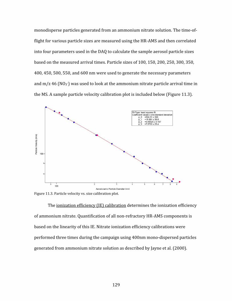
129
monodisperse particles generated from an ammonium nitrate solution. The time-of-
flight for various particle sizes are measured using the HR-AMS and then correlated
into four parameters used in the DAQ to calculate the sample aerosol particle sizes
based on the measured arrival times. Particle sizes of 100, 150, 200, 250, 300, 350,
400, 450, 500, 550, and 600 nm were used to generate the necessary parameters
and m/z 46 (NO3-) was used to look at the ammonium nitrate particle arrival time in
the MS. A sample particle velocity calibration plot is included below (Figure 11.3).
Figure 11.3. Particle velocity vs. size calibration plot.
The ionization efficiency (IE) calibration determines the ionization efficiency
of ammonium nitrate. Quantification of all non-refractory HR-AMS components is
based on the linearity of this IE. Nitrate ionization efficiency calibrations were
performed three times during the campaign using 400nm mono-dispersed particles
generated from ammonium nitrate solution as described by Jayne et al. (2000).
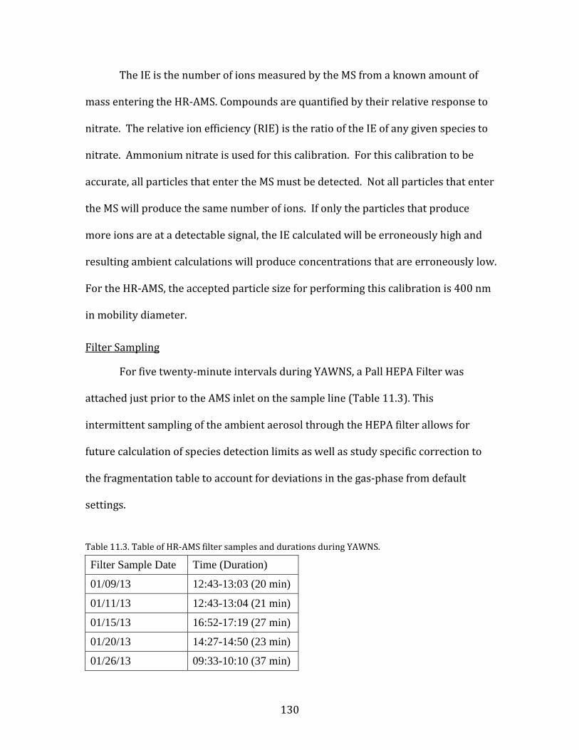
130
The IE is the number of ions measured by the MS from a known amount of
mass entering the HR-AMS. Compounds are quantified by their relative response to
nitrate. The relative ion efficiency (RIE) is the ratio of the IE of any given species to
nitrate. Ammonium nitrate is used for this calibration. For this calibration to be
accurate, all particles that enter the MS must be detected. Not all particles that enter
the MS will produce the same number of ions. If only the particles that produce
more ions are at a detectable signal, the IE calculated will be erroneously high and
resulting ambient calculations will produce concentrations that are erroneously low.
For the HR-AMS, the accepted particle size for performing this calibration is 400 nm
in mobility diameter.
Filter Sampling
For five twenty-minute intervals during YAWNS, a Pall HEPA Filter was
attached just prior to the AMS inlet on the sample line (Table 11.3). This
intermittent sampling of the ambient aerosol through the HEPA filter allows for
future calculation of species detection limits as well as study specific correction to
the fragmentation table to account for deviations in the gas-phase from default
settings.
Table 11.3. Table of HR-AMS filter samples and durations during YAWNS.
Filter Sample Date Time (Duration)
01/09/13 12:43-13:03 (20 min)
01/11/13 12:43-13:04 (21 min)
01/15/13 16:52-17:19 (27 min)
01/20/13 14:27-14:50 (23 min)
01/26/13 09:33-10:10 (37 min)
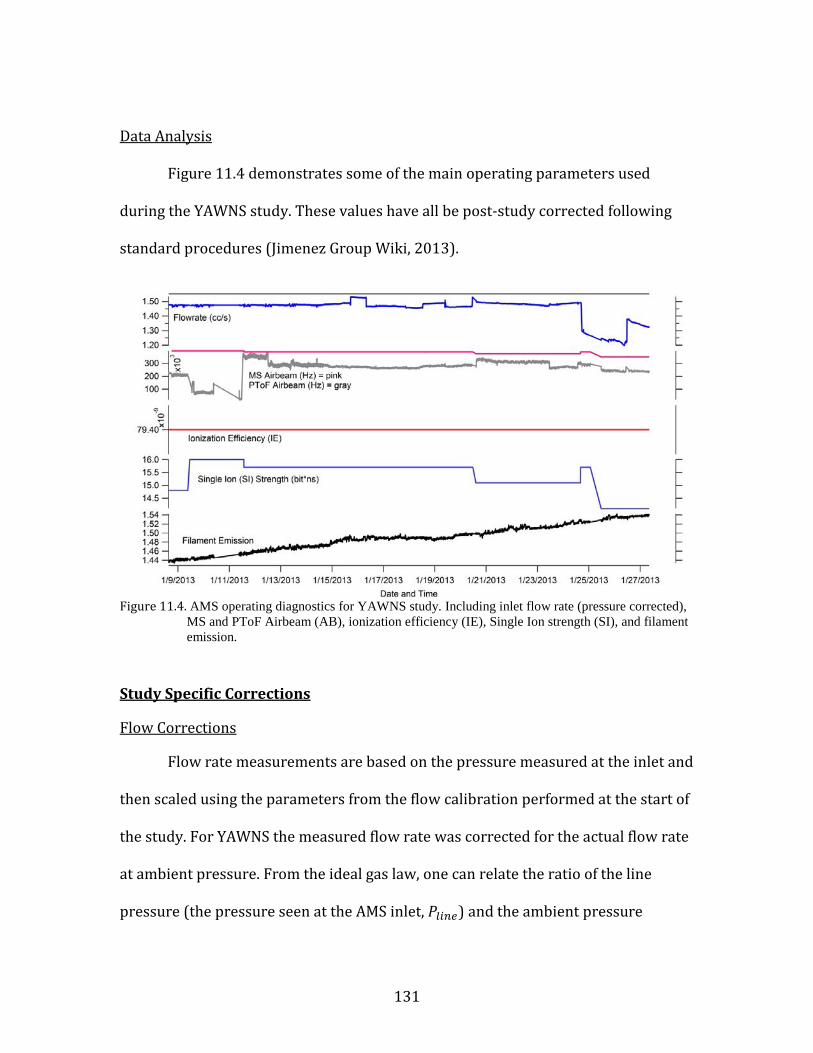
131
Data Analysis
Figure 11.4 demonstrates some of the main operating parameters used
during the YAWNS study. These values have all be post-study corrected following
standard procedures (Jimenez Group Wiki, 2013).
Figure 11.4. AMS operating diagnostics for YAWNS study. Including inlet flow rate (pressure corrected),
MS and PToF Airbeam (AB), ionization efficiency (IE), Single Ion strength (SI), and filament emission.
Study Specific Corrections Flow Corrections
Flow rate measurements are based on the pressure measured at the inlet and
then scaled using the parameters from the flow calibration performed at the start of
the study. For YAWNS the measured flow rate was corrected for the actual flow rate
at ambient pressure. From the ideal gas law, one can relate the ratio of the line
pressure (the pressure seen at the AMS inlet, 𝑃𝑙𝑖𝑛𝑒) and the ambient pressure
132
(𝑃𝑎𝑚𝑏𝑖𝑒𝑛𝑡) to the actual flow rate under ambient conditions (�̇�𝑎𝑚𝑏𝑖𝑒𝑛𝑡) and the
measured flow rate at the AMS inlet (�̇�𝑙𝑖𝑛𝑒). By making this correction measured
concentrations can be directly compared between all instrumentation.
Fragmentation Table Adjustments
The purpose of the fragmentation table is to apportion the AMS signal among
the different chemical species present in the aerosol (ammonium, chloride, nitrate,
sulfate, and organics). This table must be adjusted from study-to-study to account
for small changes between instruments and measurement environments. Most of
the necessary adjustments to the default fragmentation table have to do with air
interferences. After making the appropriate fragmentation corrections for a given
set of data the average mass spectra plots of all available filter samples are checked
to ensure that the concentration of the five main components (Org, Chl, NH4, NO3,
SO4) are each approximately zero. A more detailed explanation of the fragmentation
table is given by Allen et al. (2004).
CO2 [44]
The default mixing ratio used for the apportionment of gas-phase of CO2 in
the atmosphere is 370ppm . The amount of signal at m/z 44 (mostly CO2+) that is
due to gas phase CO2 and the amount of aerosol phase CO2+ (and other small aerosol
contributions at m/z 44) needs to be adjusted to reflect sampling conditions. Since
external measurements of gas-phase CO2 were being recorded during YAWNS, these
time-dependent measurements were used to replace the default CO2 mixing ratio.
133
Air [29]
Depending on the threshold setting and possible saturation effects, the
amount of N15N at m/z 29 detected by the system may be slightly different than that
predicted purely by an isotopic factor. In the case of this study a multiplier of 0.83
was used to adjust the predicted behavior.
Air [15]
Depending on the threshold setting and possible saturation effects, the
amount of 15N at m/z 15 detected by the system may be slightly different than that
predicted purely by an isotopic factor. In the case of this study a multiplier of 1.05
was used to adjust the predicted behavior.
O [16]
The O[16] fragment indicates the amount of gas phase signal due to O+ or a
doubly charged O22+ ion. In turn this ratio impacts the ratio of NH4[17] (NH3+) vs
NH4[16] (NH2+). This ratio should trend through the origin; since it did not a
multiplier of 0.7 was used to correct the ratio so that the data would trend through
the origin.
11.3. NOx/NOy Analyzer Operation and Calibration
The principal of measurement for this instrument is chemiluminescence,
where NO reacts with ozone to produce a vibrationally excited NO2 molecule:
NO + O3 NO2* + O2 [Rxn 11.1].
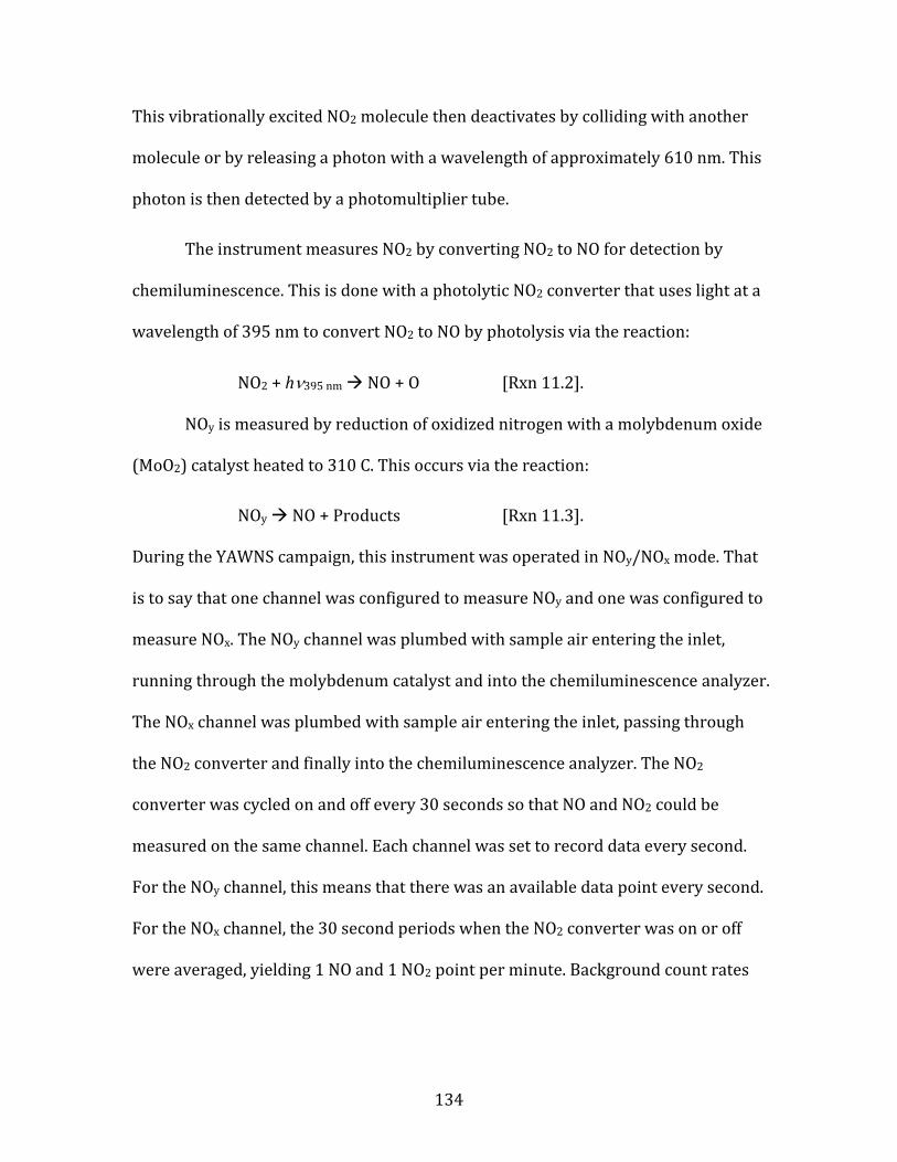
134
This vibrationally excited NO2 molecule then deactivates by colliding with another
molecule or by releasing a photon with a wavelength of approximately 610 nm. This
photon is then detected by a photomultiplier tube.
The instrument measures NO2 by converting NO2 to NO for detection by
chemiluminescence. This is done with a photolytic NO2 converter that uses light at a
wavelength of 395 nm to convert NO2 to NO by photolysis via the reaction:
NO2 + hν395 nm NO + O [Rxn 11.2].
NOy is measured by reduction of oxidized nitrogen with a molybdenum oxide
(MoO2) catalyst heated to 310 C. This occurs via the reaction:
NOy NO + Products [Rxn 11.3].
During the YAWNS campaign, this instrument was operated in NOy/NOx mode. That
is to say that one channel was configured to measure NOy and one was configured to
measure NOx. The NOy channel was plumbed with sample air entering the inlet,
running through the molybdenum catalyst and into the chemiluminescence analyzer.
The NOx channel was plumbed with sample air entering the inlet, passing through
the NO2 converter and finally into the chemiluminescence analyzer. The NO2
converter was cycled on and off every 30 seconds so that NO and NO2 could be
measured on the same channel. Each channel was set to record data every second.
For the NOy channel, this means that there was an available data point every second.
For the NOx channel, the 30 second periods when the NO2 converter was on or off
were averaged, yielding 1 NO and 1 NO2 point per minute. Background count rates
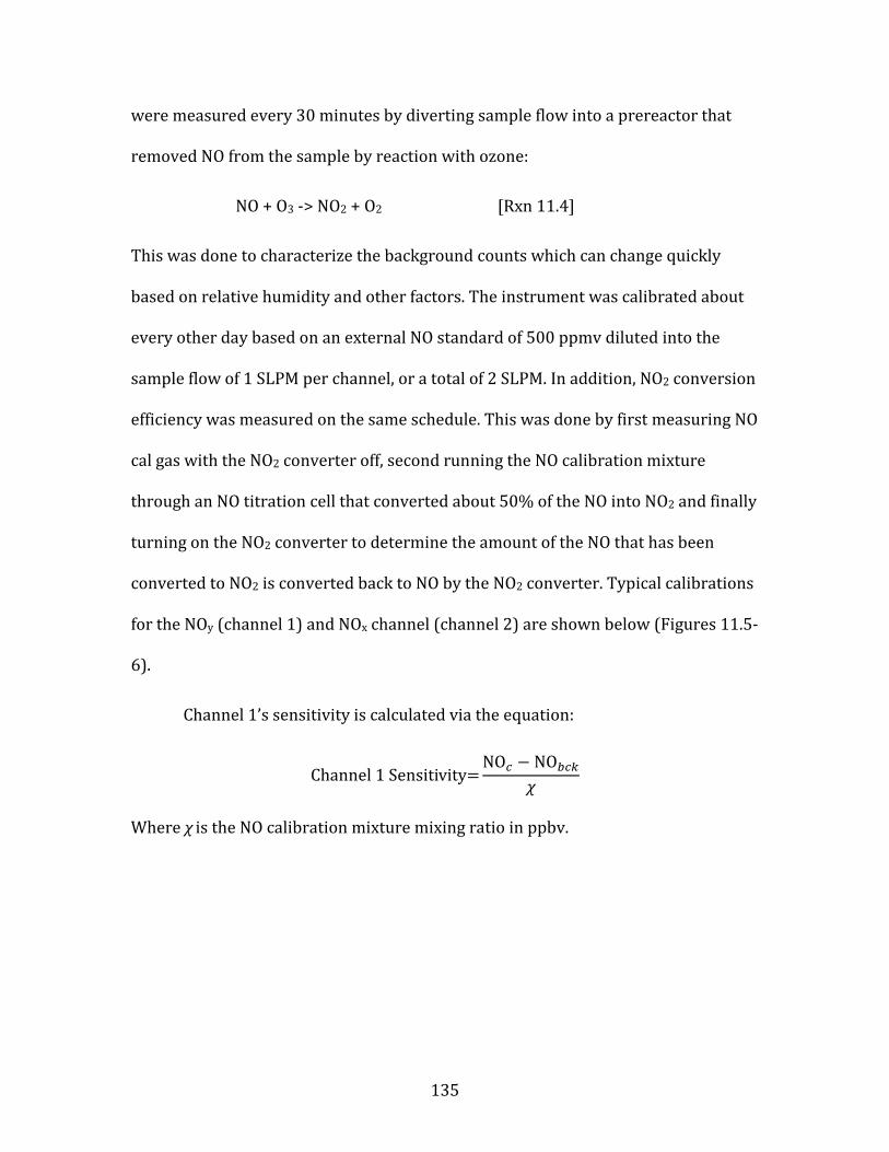
135
were measured every 30 minutes by diverting sample flow into a prereactor that
removed NO from the sample by reaction with ozone:
NO + O3 -> NO2 + O2 [Rxn 11.4]
This was done to characterize the background counts which can change quickly
based on relative humidity and other factors. The instrument was calibrated about
every other day based on an external NO standard of 500 ppmv diluted into the
sample flow of 1 SLPM per channel, or a total of 2 SLPM. In addition, NO2 conversion
efficiency was measured on the same schedule. This was done by first measuring NO
cal gas with the NO2 converter off, second running the NO calibration mixture
through an NO titration cell that converted about 50% of the NO into NO2 and finally
turning on the NO2 converter to determine the amount of the NO that has been
converted to NO2 is converted back to NO by the NO2 converter. Typical calibrations
for the NOy (channel 1) and NOx channel (channel 2) are shown below (Figures 11.5-
6).
Channel 1’s sensitivity is calculated via the equation:
Channel 1 Sensitivity=NO𝑐 − NO𝑏𝑐𝑘
𝜒
Where χ is the NO calibration mixture mixing ratio in ppbv.
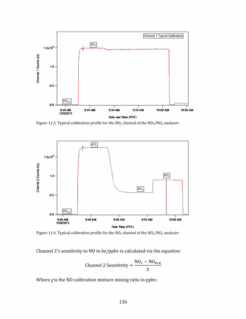
136
Figure 11.5. Typical calibration profile for the NOy channel of the NOx/NOy analyzer.
Figure 11.6. Typical calibration profile for the NOx channel of the NOx/NOy analyzer.
Channel 2’s sensitivity to NO in hz/ppbv is calculated via the equation:
Channel 2 Sensitivity =NO𝑐 − NO𝑏𝑐𝑘
χ
Where χ is the NO calibration mixture mixing ratio in ppbv.
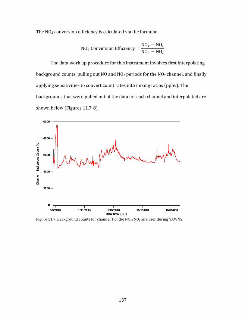
137
The NO2 conversion efficiency is calculated via the formula:
NO2 Conversion Ef�iciency =NO𝑥 − NO𝐿
NO𝐶 − NO𝐿
The data work up procedure for this instrument involves first interpolating
background counts, pulling out NO and NO2 periods for the NOx channel, and finally
applying sensitivities to convert count rates into mixing ratios (ppbv). The
backgrounds that were pulled out of the data for each channel and interpolated are
shown below (Figures 11.7-8).
Figure 11.7. Background counts for channel 1 of the NOx/NOy analyzer during YAWNS.
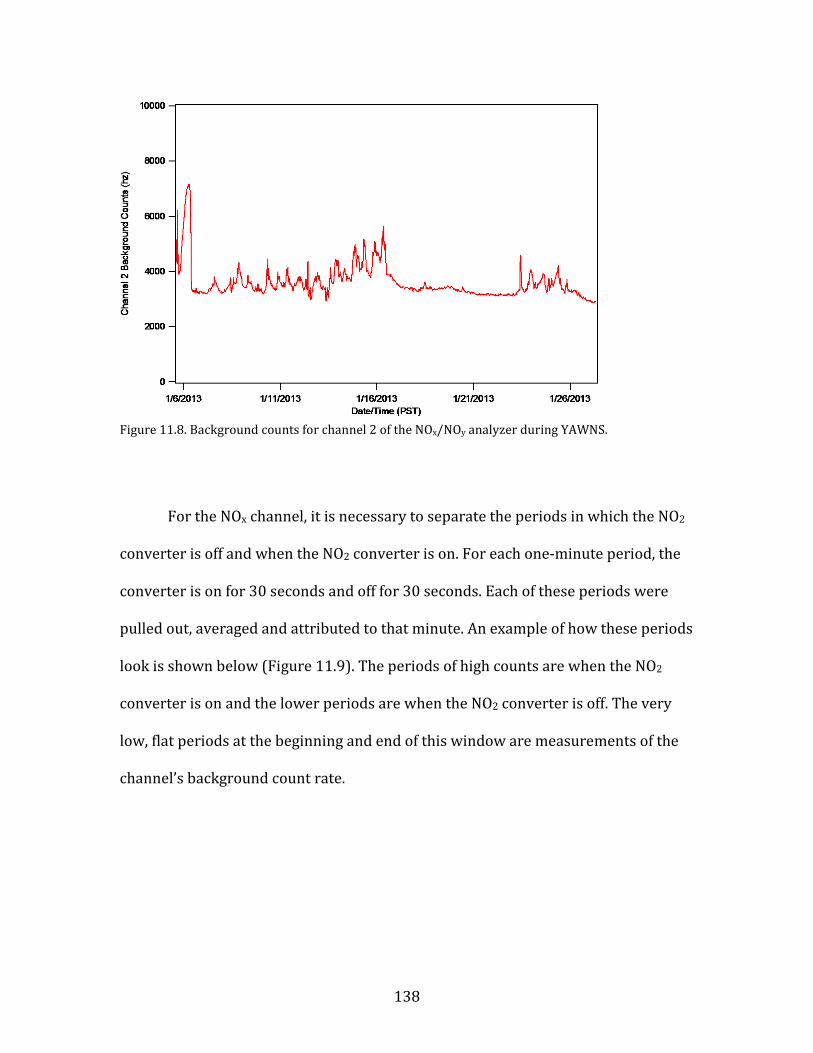
138
Figure 11.8. Background counts for channel 2 of the NOx/NOy analyzer during YAWNS.
For the NOx channel, it is necessary to separate the periods in which the NO2
converter is off and when the NO2 converter is on. For each one-minute period, the
converter is on for 30 seconds and off for 30 seconds. Each of these periods were
pulled out, averaged and attributed to that minute. An example of how these periods
look is shown below (Figure 11.9). The periods of high counts are when the NO2
converter is on and the lower periods are when the NO2 converter is off. The very
low, flat periods at the beginning and end of this window are measurements of the
channel’s background count rate.

139
Figure 11.9. Representative time series of the raw count rate measured by channel 2 of the NOx/NOy
analyzer. Explanation provided in the text.
To calculate NOy mixing ratios, the interpolated background of channel 1 is
simply subtracted from the overall channel 1 count rate and then divided by the
sensitivity. This assumes that the conversion efficiency of the catalyst is 1.
NO𝑦 (ppbv) =CH1 (hz) − CH1𝑏𝑐𝑘 (hz)
CH1𝑠𝑒𝑛𝑠 � hzppbv
�
Where CH1 is the signal of channel 1, CH1bck is the interpolated background, and
CH1sens is the sensitivity of channel 1. To calculate NO mixing ratios, the interpolated
background of channel 2 is subtracted from the NO period averages and then
divided by the channel 2 sensitivity.
NO (ppbv) =CH2𝑁𝑂 (hz) − CH2𝑏𝑐𝑘 (hz)
CH2𝑠𝑒𝑛𝑠 � hzppbv
�
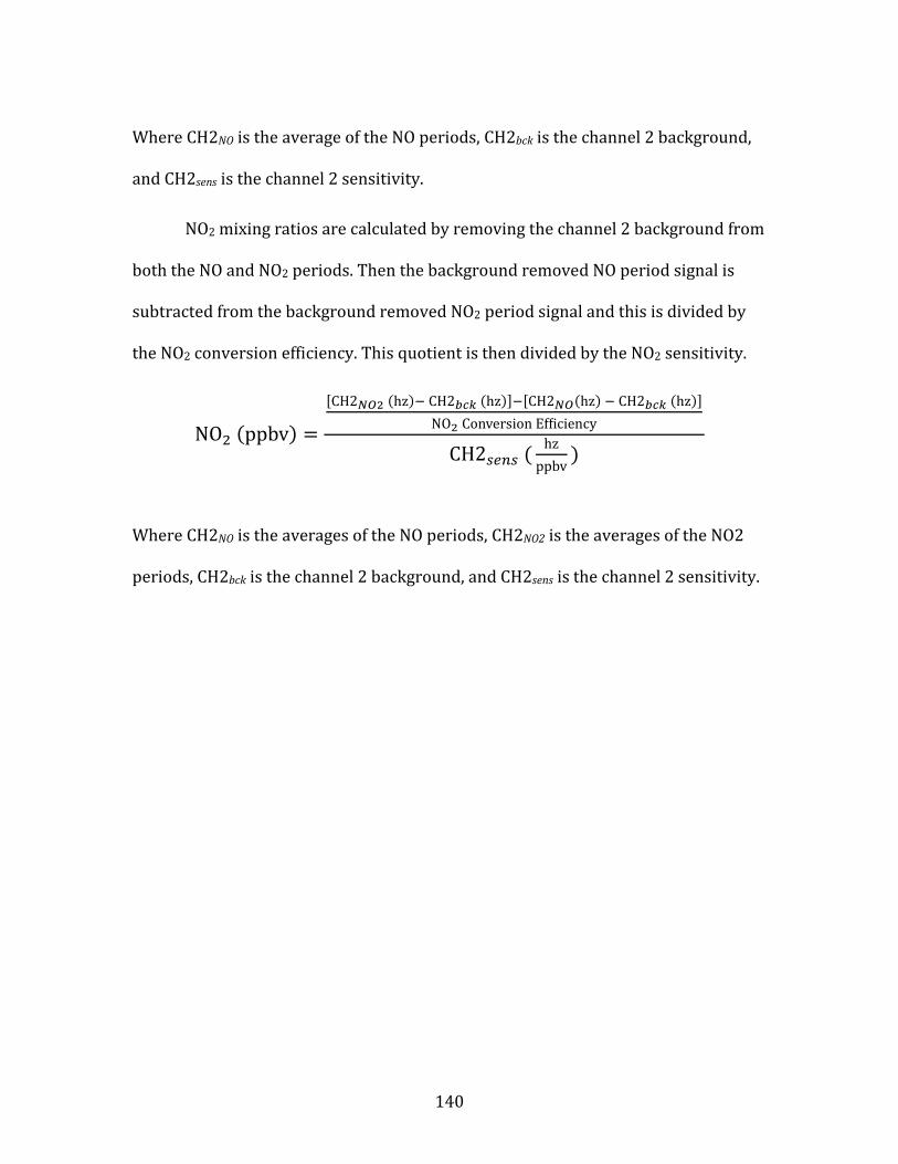
140
Where CH2NO is the average of the NO periods, CH2bck is the channel 2 background,
and CH2sens is the channel 2 sensitivity.
NO2 mixing ratios are calculated by removing the channel 2 background from
both the NO and NO2 periods. Then the background removed NO period signal is
subtracted from the background removed NO2 period signal and this is divided by
the NO2 conversion efficiency. This quotient is then divided by the NO2 sensitivity.
NO2 (ppbv) =
[CH2𝑁𝑂2 (hz)− CH2𝑏𝑐𝑘 (hz)]−[CH2𝑁𝑂(hz) − CH2𝑏𝑐𝑘 (hz)]NO2 Conversion Ef�iciency
CH2𝑠𝑒𝑛𝑠 ( hzppbv
)
Where CH2NO is the averages of the NO periods, CH2NO2 is the averages of the NO2
periods, CH2bck is the channel 2 background, and CH2sens is the channel 2 sensitivity.
141
11.4. Aerolaser VUV CO Instrument Operation and Calibration
In the field, the Aerolaser VUV CO instrument was configured to report data
every second. Background count rates were measured every four hours by passing
sample air through a SOFNOCAT 514 scrubber, which removes any CO from the
sample. Calibrations were also done every 4 hours by mixing about 30 SCCM of an
external CO standard of 101.6 ppmv in to the typical sample flow of approximately
800 SCCM. To account for ambient CO, ambient air is measured with no calibration
(cal) gas addition before and after cal gas is measured. The average of these two
periods is subtracted from the count rate observed when cal gas is introduced to
determine the count rate that is attributable to only the cal gas. A typical
background/calibration goes as follows: ambient air through SOFNOCAT 515
(instrument background), measure ambient air (calibration background 1), ambient
sample with calibration gas added (calibration), and finally ambient air is measured
again (calibration background 2). A typical calibration is shown below (Figure
11.10).
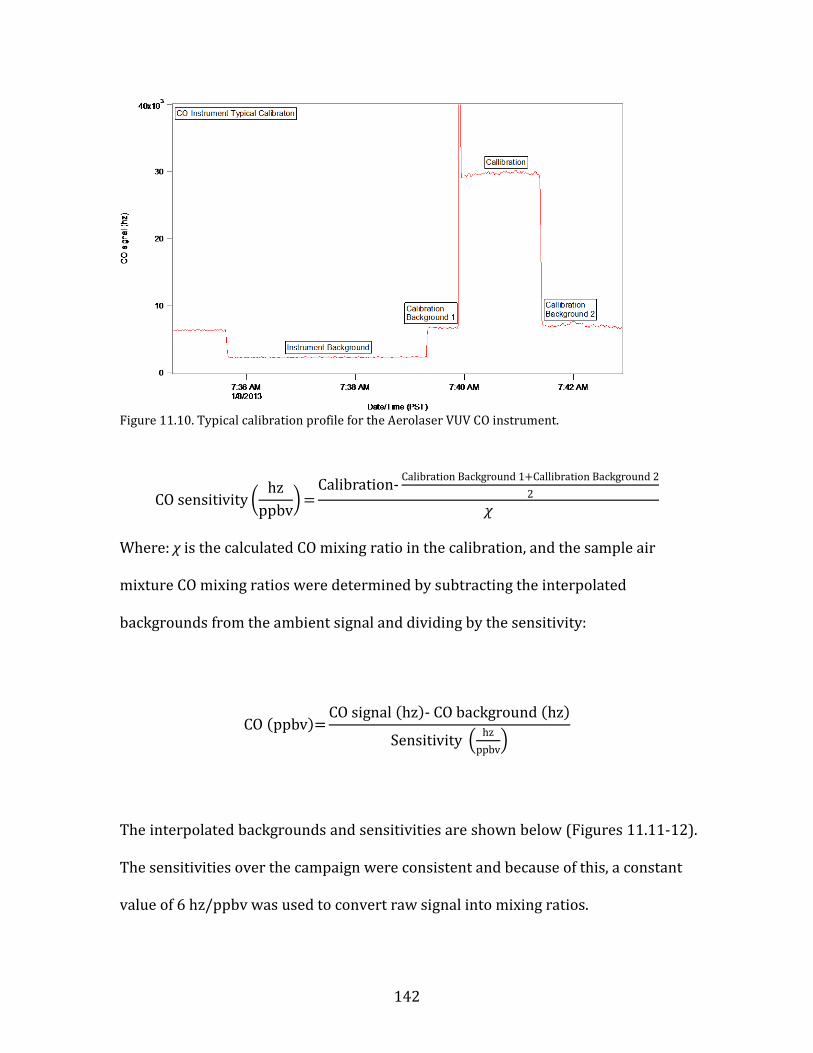
142
Figure 11.10. Typical calibration profile for the Aerolaser VUV CO instrument.
CO sensitivity �hz
ppbv� =
Calibration- Calibration Background 1+Callibration Background 22
𝜒
Where: χ is the calculated CO mixing ratio in the calibration, and the sample air
mixture CO mixing ratios were determined by subtracting the interpolated
backgrounds from the ambient signal and dividing by the sensitivity:
CO (ppbv)=CO signal (hz)- CO background (hz)
Sensitivity � hzppbv
�
The interpolated backgrounds and sensitivities are shown below (Figures 11.11-12).
The sensitivities over the campaign were consistent and because of this, a constant
value of 6 hz/ppbv was used to convert raw signal into mixing ratios.
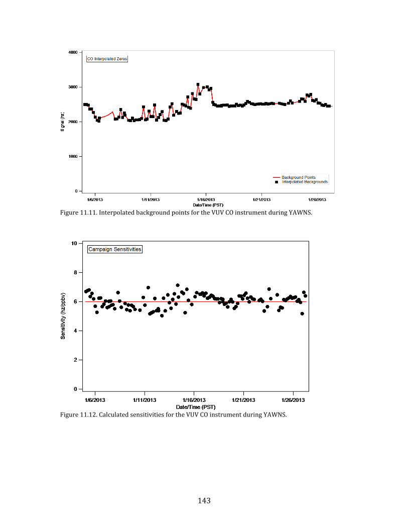
143
Figure 11.11. Interpolated background points for the VUV CO instrument during YAWNS.
Figure 11.12. Calculated sensitivities for the VUV CO instrument during YAWNS.
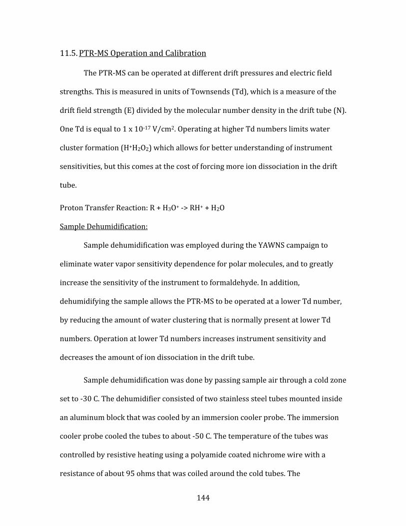
144
11.5. PTR-MS Operation and Calibration
The PTR-MS can be operated at different drift pressures and electric field
strengths. This is measured in units of Townsends (Td), which is a measure of the
drift field strength (E) divided by the molecular number density in the drift tube (N).
One Td is equal to 1 x 10-17 V/cm2. Operating at higher Td numbers limits water
cluster formation (H+H2O2) which allows for better understanding of instrument
sensitivities, but this comes at the cost of forcing more ion dissociation in the drift
tube.
Proton Transfer Reaction: R + H3O+ -> RH+ + H2O Sample Dehumidification:
Sample dehumidification was employed during the YAWNS campaign to
eliminate water vapor sensitivity dependence for polar molecules, and to greatly
increase the sensitivity of the instrument to formaldehyde. In addition,
dehumidifying the sample allows the PTR-MS to be operated at a lower Td number,
by reducing the amount of water clustering that is normally present at lower Td
numbers. Operation at lower Td numbers increases instrument sensitivity and
decreases the amount of ion dissociation in the drift tube.
Sample dehumidification was done by passing sample air through a cold zone
set to -30 C. The dehumidifier consisted of two stainless steel tubes mounted inside
an aluminum block that was cooled by an immersion cooler probe. The immersion
cooler probe cooled the tubes to about -50 C. The temperature of the tubes was
controlled by resistive heating using a polyamide coated nichrome wire with a
resistance of about 95 ohms that was coiled around the cold tubes. The
145
temperatures of the individual tubes were controlled by Watlow temperature
controllers and the tube temperature was measured continuously using a
thermocouple probe that was in contact with the inner wall of the tube.
In the field, the two tubes were operated in tandem so that measurements
would remain continuous over the course of the campaign. Each tube operated in
one of three states at any given time; sample, condition, or backflush. Sample mode
was when ambient air was sampled by the PTR-MS through the cold tube. In
backflush mode, the tube was heated up to 70 C and flush with dry N2 to remove ice
buildup that may have formed while sampling. Conditioning mode is when the tube
is returned to the low temperature with ambient air flowing through before being
used as a dehumidifier for the PTR-MS sample. At any given time, one tube was in
sample mode, while the other was in the process of being backflushed and
conditioned. This cycle was 20 minutes long, so each tube was used to dehumidify
sample air for 20 minutes before being backflushed and reconditioned. This process
was automated so that continuous measurements could be made without operators
present.
IVOC Sampler:
Between January 12 and January 24, a thermal desorption system was used
in conjunction with the PTR-MS to measure larger molecular weight VOC that were
below the detection limit of the instrument. This system employed a Tenax trap to
accumulate VOCs over a 20-minute sampling period while the PTR-MS was
measuring ambient air. VOCs were desorbed and measured by the PTR-MS for 5-
minute periods, during which the PTR-MS was not making ambient measurements.
146
Because of an issue of the sample line not being continuously conditioned, the IVOC
data will not be presented in this report. However, being that the IVOC sampling
cycle lasted about 30 minutes and the IVOC measure mode when the PTR-MS is not
measuring ambient air lasted 5 minutes, it is important to note that 5 of every
approximately 30 minutes of VOC sampling was lost.
In Field Operation:
During the measurement campaign, The PTR-MS was operated in one of
three modes: 120 Td VOC mode, 80 Td VOC mode, and 80 Td VOC and IVOC mode.
120 Td VOC mode was when the PTR-MS sampled ambient air at 120 Td without
dehumidifying the sample, 80 Td VOC mode was when the PTR-MS measured
ambient air at 80 Td through the dehumidifier, and 80 Td VOC and IVOC mode was
when the PTR-MS measured ambient air at 80 Td, but the thermal desorption
sampler was also running and desorbing for PTR-MS measurements for 5 of every
30 minutes. Table 11.4 below shows operation modes during the different intervals
of the study.
Table 11.4. PTR-MS operation modes during YAWNS. Date Td Dehumidification IVOC system
1/5 – 1/8 120 NO NO 1/8 – 1/12 80 YES NO
1/12 – 1/24 80 YES YES 1/24 – 1/27 120 NO NO
Calibration and Sensitivities:
The PTR-MS was calibrated 8 times over the course of the study. This was
done by sampling about 10 SCCM of an external gas standard dilluted with
approximately 1 SLPM of zero air. Backgrounds were also taken by measuring zero
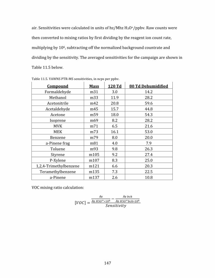
147
air. Sensitivities were calculated in units of hz/Mhz H3O+/ppbv. Raw counts were
then converted to mixing ratios by first dividing by the reagent ion count rate,
multiplying by 106, subtracting off the normalized background countrate and
dividing by the sensitivity. The averaged sensitivities for the campaign are shown in
Table 11.5 below.
Table 11.5. YAWNS PTR-MS sensitivities, in ncps per ppbv.
Compound Mass 120 Td 80 Td Dehumidified Formaldehyde m31 3.0 14.2
Methanol m33 11.9 28.2 Acetonitrile m42 20.8 59.6
Acetaldehyde m45 15.7 44.8 Acetone m59 18.0 54.3 Isoprene m69 8.2 28.2
MVK m71 6.5 21.6 MEK m73 16.1 53.0
Benzene m79 8.0 20.0 a-Pinene frag m81 4.0 7.9
Toluene m93 9.8 26.3 Styrene m105 9.2 27.4
P-Xylene m107 8.3 25.0 1,2,4-Trimethylbenzene m121 6.6 20.3
Teramethylbenzene m135 7.3 22.5 a-Pinene m137 2.6 10.8
VOC mixing ratio calculation:
[𝑉𝑂𝐶] =ℎ𝑧
ℎ𝑧 𝐻3𝑂+∗106 − ℎ𝑧 𝑏𝑐𝑘ℎ𝑧 𝐻3𝑂+𝑏𝑐𝑘∗106
𝑆𝑒𝑛𝑠𝑖𝑡𝑖𝑣𝑖𝑡𝑦
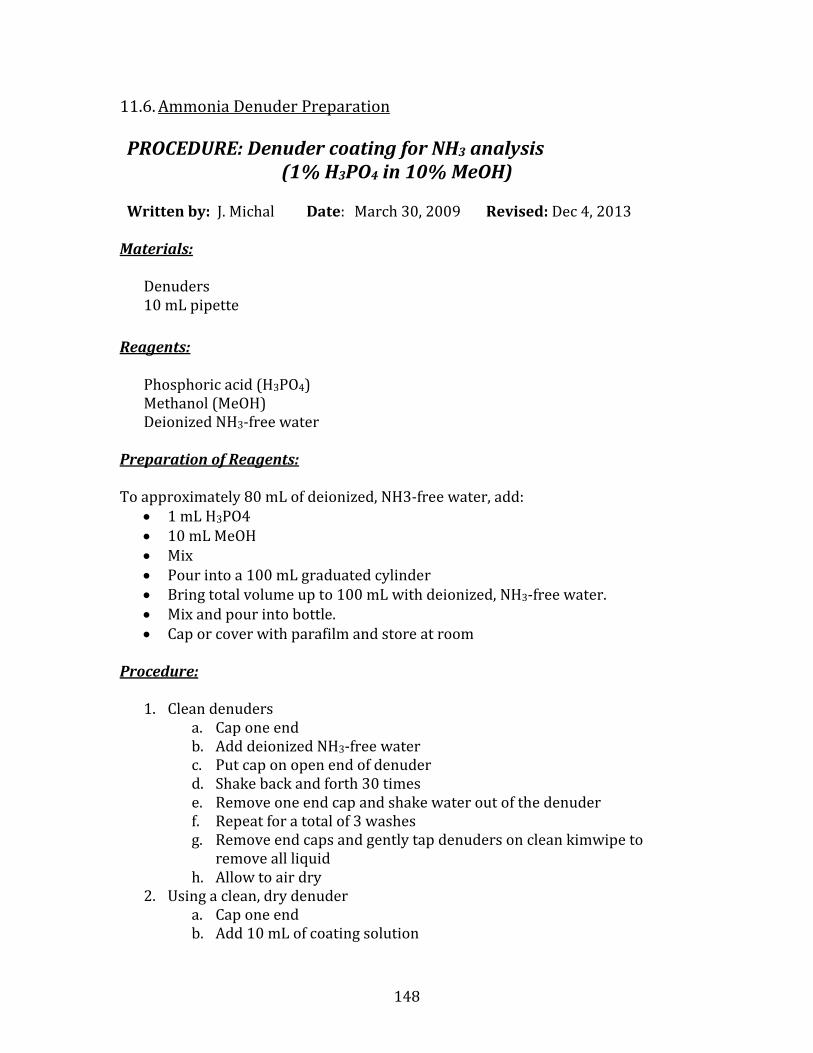
148
11.6. Ammonia Denuder Preparation
PROCEDURE: Denuder coating for NH3 analysis (1% H3PO4 in 10% MeOH)
Written by: J. Michal
Date: March 30, 2009
Revised: Dec 4, 2013
Materials:
Denuders 10 mL pipette
Reagents:
Phosphoric acid (H3PO4) Methanol (MeOH) Deionized NH3-free water
Preparation of Reagents: To approximately 80 mL of deionized, NH3-free water, add:
• 1 mL H3PO4 • 10 mL MeOH • Mix • Pour into a 100 mL graduated cylinder • Bring total volume up to 100 mL with deionized, NH3-free water. • Mix and pour into bottle. • Cap or cover with parafilm and store at room
Procedure:
1. Clean denuders a. Cap one end b. Add deionized NH3-free water c. Put cap on open end of denuder d. Shake back and forth 30 times e. Remove one end cap and shake water out of the denuder f. Repeat for a total of 3 washes g. Remove end caps and gently tap denuders on clean kimwipe to
remove all liquid h. Allow to air dry
2. Using a clean, dry denuder a. Cap one end b. Add 10 mL of coating solution

149
c. Put cap with hole in end on the open end of the denuder d. Shake back and forth 30 times e. Remove end cap with the hole and tap denuder into plastic funnel
placed on waste collection bottle. Tap gently until all liquid has been removed
f. Tap denuder on clean kimwipe to remove any liquid g. Dry with nitrogen gas or zero air
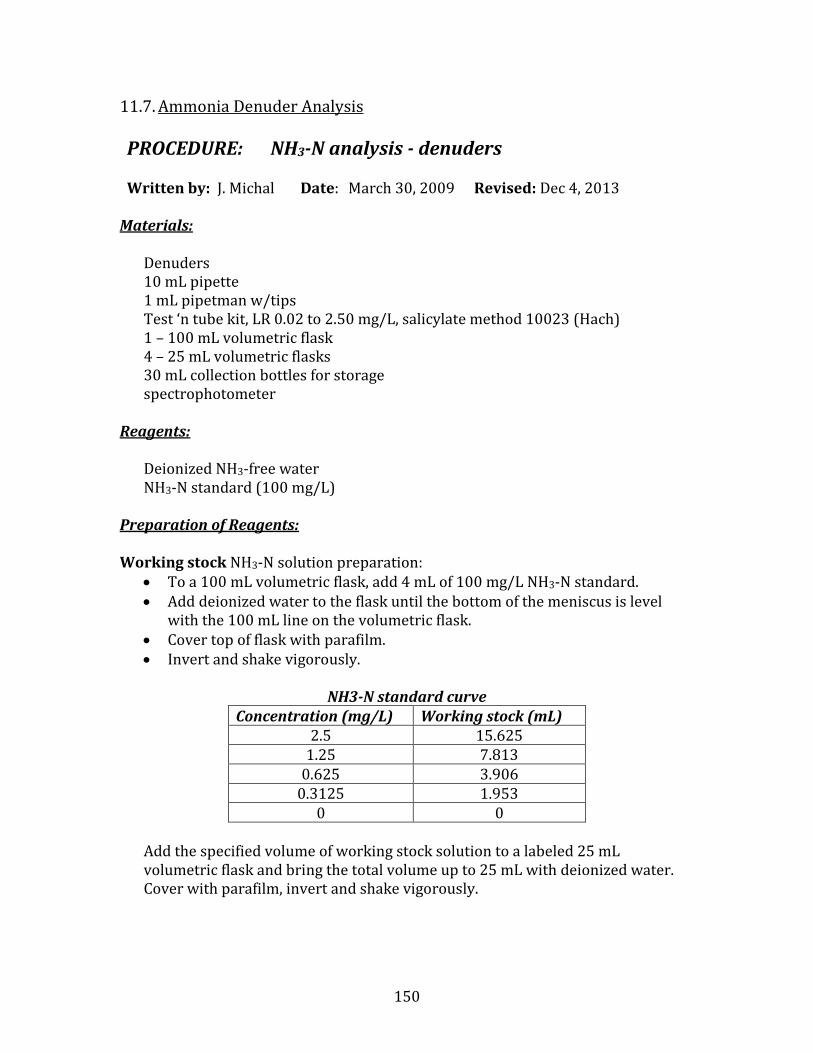
150
11.7. Ammonia Denuder Analysis
PROCEDURE: NH3-N analysis - denuders Written by: J. Michal
Date: March 30, 2009
Revised: Dec 4, 2013
Materials:
Denuders 10 mL pipette 1 mL pipetman w/tips Test ‘n tube kit, LR 0.02 to 2.50 mg/L, salicylate method 10023 (Hach) 1 – 100 mL volumetric flask 4 – 25 mL volumetric flasks 30 mL collection bottles for storage spectrophotometer
Reagents:
Deionized NH3-free water NH3-N standard (100 mg/L)
Preparation of Reagents: Working stock NH3-N solution preparation:
• To a 100 mL volumetric flask, add 4 mL of 100 mg/L NH3-N standard. • Add deionized water to the flask until the bottom of the meniscus is level
with the 100 mL line on the volumetric flask. • Cover top of flask with parafilm. • Invert and shake vigorously.
NH3-N standard curve
Concentration (mg/L) Working stock (mL) 2.5 15.625
1.25 7.813 0.625 3.906
0.3125 1.953 0 0
Add the specified volume of working stock solution to a labeled 25 mL volumetric flask and bring the total volume up to 25 mL with deionized water. Cover with parafilm, invert and shake vigorously.
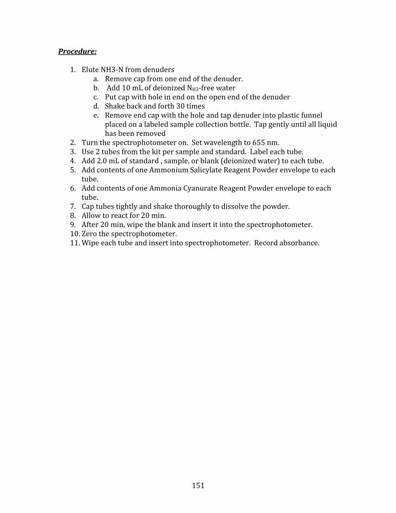
151
Procedure:
1. Elute NH3-N from denuders a. Remove cap from one end of the denuder. b. Add 10 mL of deionized NH3-free water c. Put cap with hole in end on the open end of the denuder d. Shake back and forth 30 times e. Remove end cap with the hole and tap denuder into plastic funnel
placed on a labeled sample collection bottle. Tap gently until all liquid has been removed
2. Turn the spectrophotometer on. Set wavelength to 655 nm. 3. Use 2 tubes from the kit per sample and standard. Label each tube. 4. Add 2.0 mL of standard , sample, or blank (deionized water) to each tube. 5. Add contents of one Ammonium Salicylate Reagent Powder envelope to each
tube. 6. Add contents of one Ammonia Cyanurate Reagent Powder envelope to each
tube. 7. Cap tubes tightly and shake thoroughly to dissolve the powder. 8. Allow to react for 20 min. 9. After 20 min, wipe the blank and insert it into the spectrophotometer. 10. Zero the spectrophotometer. 11. Wipe each tube and insert into spectrophotometer. Record absorbance.