theoretical computer sciencem. dalla preda et al. / theoretical computer science 577 (2015) 74–97...
TRANSCRIPT
Theoretical Computer Science 577 (2015) 74–97
Contents lists available at ScienceDirect
Theoretical Computer Science
www.elsevier.com/locate/tcs
Unveiling metamorphism by abstract interpretation of code
properties
Mila Dalla Preda a,∗, Roberto Giacobazzi a, Saumya Debray b
a University of Verona, Italyb University of Arizona, USA
a r t i c l e i n f o a b s t r a c t
Article history:Received 13 November 2012Received in revised form 10 May 2014Accepted 17 February 2015Available online 23 February 2015Communicated by V. Sassone
Keywords:Abstract interpretationProgram semanticsMetamorphic malware detectionSelf-modifying programs
Metamorphic code includes self-modifying semantics-preserving transformations to exploit code diversification. The impact of metamorphism is growing in security and code protection technologies, both for preventing malicious host attacks, e.g., in software diversification for IP and integrity protection, and in malicious software attacks, e.g., in metamorphic malware self-modifying their own code in order to foil detection systems based on signature matching. In this paper we consider the problem of automatically extracting metamorphic signatures from metamorphic code. We introduce a semantics for self-modifying code, later called phase semantics, and prove its correctness by showing that it is an abstract interpretation of the standard trace semantics. Phase semantics precisely models the metamorphic code behavior by providing a set of traces of programs which correspond to the possible evolutions of the metamorphic code during execution. We show that metamorphic signatures can be automatically extracted by abstract interpretation of the phase semantics. In particular, we introduce the notion of regular metamorphism, where the invariants of the phase semantics can be modeled as finite state automata representing the code structure of all possible metamorphic change of a metamorphic code, and we provide a static signature extraction algorithm for metamorphic code where metamorphic signatures are approximated in regular metamorphism.
© 2015 Elsevier B.V. All rights reserved.
1. Introduction
Detecting and neutralizing computer malware, such as worms, viruses, trojans, and spyware is a major challenge in modern computer security, involving both sophisticated intrusion detection strategies and advanced code manipulation tools and methods. Traditional misuse malware detectors (also known as signature-based detectors) are typically syntactic in nature: they use pattern matching to compare the byte sequence comprising the body of the malware against a signature database [34]. Malware writers have responded by using a variety of techniques in order to avoid detection: Encryption, oligomorphism with mutational decryption patterns, and polymorphism with different encryption methods for generat-ing an endless sequence of decryption patterns are typical strategies for achieving malware diversification. Metamorphism emerged in the last decade as an effective alternative strategy to foil misuse malware detectors. Metamorphic malware apply semantics-preserving transformations to modify its own code so that one instance of the malware bears very little resemblance to another instance, in a kind of body-polymorphism [33], even though semantically their functionality is the
* Corresponding author.E-mail addresses: [email protected] (M. Dalla Preda), [email protected] (R. Giacobazzi), [email protected] (S. Debray).
http://dx.doi.org/10.1016/j.tcs.2015.02.0240304-3975/© 2015 Elsevier B.V. All rights reserved.
M. Dalla Preda et al. / Theoretical Computer Science 577 (2015) 74–97 75
same. Thus, a metamorphic malware is a malware equipped with a metamorphic engine that takes the malware, or parts of it, as input and morphs it at run-time to a syntactically different but semantically equivalent variant, in order to avoid de-tection. Some of the basic metamorphic transformations commonly used by malware are semantic-nop/junk insertion, code permutation, register swap and substitution of equivalent sequences of instructions [7,33]. It is worth noting that most of these transformations can be seen as special cases of code substitution [23]. The quantity of metamorphic variants possible for a particular piece of malware makes it impractical to maintain a signature set that is large enough to cover most or all of these variants, making standard signature-based detection ineffective [10]. Existing malware detectors therefore fall back on a variety of heuristic techniques, but these may be prone to false positives (where innocuous files are mistakenly identified as malware) or false negatives (where malware escape detection) at worst. The reason for this vulnerability to metamorphism lies upon the purely syntactic nature of most existing and commercial detectors. The key for identifying metamorphic malware lies, instead, in a deeper understanding of their semantics. Preliminary works in this direction by Dalla Preda et al. [16], Christodorescu et al. [11], and Kinder et al. [27] confirm the potential benefits of a semantics-based approach to malware detection. Still a major drawback of existing semantics-based methods relies upon their need of an a priori knowledge of the obfuscations used to implement the metamorphic engine. Because of this, it is always possible for any expert malware writer to develop alternative metamorphic strategies, even by simple modification of existing ones, able to foil any given detection scheme. Indeed, handling metamorphism represents one of the main challenges in modern malware analysis and detection [18].
Contributions We use the term metamorphic signature to refer to an abstract program representation that ideally captures all the possible code variants that might be generated during the execution of a metamorphic program. A metamorphic signature is therefore any (possibly decidable) approximation of the properties of code evolution. We propose a different approach to metamorphic malware detection based on the idea that extracting metamorphic signatures is approximating mal-ware semantics. Program semantics concerns here the way code changes, i.e., the effect of instructions that modify other instructions. We face the problem of determining how code mutates, by catching properties of this mutation, without any a priori knowledge about the implementation of the metamorphic transformations. We use a formal semantics to model the execution behavior of self-modifying code commonly encountered in malware. Using this as the basis, we propose a theo-retical model for statically deriving, by abstract interpretation, an abstract specification of all possible code variants that can be generated during the execution of a metamorphic malware. Traditional static analysis techniques are not adequate for this purpose, as they typically assume that programs do not change during execution. We therefore define a more general semantics-based behavioral model, called phase semantics, that can cope with changes to the program code at run time. The idea is to partition each possible execution trace of a metamorphic program into phases, each collecting the computations performed by a particular code variant. The sequence of phases (once disassembled) represents the sequence of possible code mutations, while the sequence of states within a given phase represents the behavior of a particular code variant.
Phase semantics precisely expresses all the possible phases, namely code variants, that can be generated during the execution of a metamorphic code. Phase semantics can then be used as a metamorphic signature for checking whether a program is a metamorphic variant of another one. Indeed, thanks to the precision of phase semantics, we have that a program Q is a metamorphic variant of a program P if and only if Q appears in the phase semantics of P . Unfortunately, due to the possible infinite sequences of code variants that can be present in the phase semantics of P , the above test for metamorphism is undecidable in general. Thus, in order to gain decidability, we need to loose precision and do so by using the well established theory of abstract interpretation [12,13]. Indeed, abstract interpretation is used here to extract the invariant properties of phases, which are properties of the generated program variants. Abstract domains represent here properties of the code shape in phases. We use the domain of finite state automata (FSA) for approximating phases and provide a static semantics of traces of FSA as an abstraction of the phase semantics. We introduce the notion of regular metamorphism as a further approximation obtained by abstracting sequences of FSA into a single FSA. This abstraction provides an upper regular language-based approximation of any metamorphic behavior of a program and it leads to a decidable test for metamorphism. This is particularly suitable to extract metamorphic signatures for engines implemented themselves as FSA of basic code transformations, which correspond to the way most classical metamorphic generators are implemented [23,31,35]. Our approach is general and language independent, providing an adequate theoretical foundation for the systematic design of algorithms and methods devoted to the extraction of approximate metamorphic signatures from any metamorphic code P . The main advantage of the phase semantics here is in modeling code mutations without isolating the metamorphic engine from the rest of the viral code. The approximation of the phase semantics by abstract interpretation can make decidable whether a given binary matches a metamorphic signature, without knowing any features of the metamorphic engine itself.
Structure of the paper In Section 3 we describe the behavior of a metamorphic program as a graph, later called program evolution graph, where each vertex is a standard static representation of programs (e.g., a control flow graph) and whose edges represent possible run-time changes to the code. We then define the phase semantics of a program as the set of all possible paths in the program evolution graph and we prove its correctness by showing that it is a sound abstract interpretation of standard trace semantics. Thus, phase semantics provides a precise description of the history of run-time code modifications, namely the sequences of “code snapshots” that can be generated during execution. Then, in Section 4, we introduce a general method for extracting metamorphic signatures as abstract interpretation of phase semantics. The result
76 M. Dalla Preda et al. / Theoretical Computer Science 577 (2015) 74–97
of the analysis is a correct approximate specification of the malware evolution, namely an approximated representation of all its possible metamorphic variants. This method is instantiated in Section 5 by abstracting programs with FSA over the alphabet of abstract binary instructions and phase semantics by sequences of FSA. Here, the abstract phase semantics is given by a set of sequences of FSA and it provides a behavioral model for the evolution of any metamorphic program. Next, in Section 6, we introduce regular metamorphism modeling metamorphic engines as FSA of basic code transformations. This is achieved by approximating the phase semantics of program P as a unique FSA W� P �, whose language contains the strings of instructions that corresponds to the runs of all the metamorphic variants of P . W� P � provides an approximated metamorphic signature of P which can be used to verify whether a program is a metamorphic variant of P by language inclusion which is decidable for regular languages. In Section 7 we discuss how the presented approach could be applied to the analysis of the metamorphic virus MetaPHOR. The paper ends with a discussion and related works.
The results presented in this work are an extended and reviewed version of [17].
2. Background
Mathematical notation Given two sets S and T , we denote with ℘(S) the powerset of S , with S � T the set-difference between S and T , with S ⊂ T strict inclusion and with S ⊆ T inclusion. Let S⊥ be set S augmented with the undefined value ⊥, i.e., S⊥ = S ∪ {⊥}. 〈P , ≤〉 denotes a poset P with ordering relation ≤, while 〈P , ≤, ∨, ∧, �, ⊥〉 denotes a complete lattice P , with ordering ≤, least upper bound (lub) ∨, greatest lower bound (glb) ∧, greatest element (top) �, and least element (bottom) ⊥. Often, ≤P will be used to denote the underlying ordering of a poset P , and ∨P , ∧P , �P and ⊥Pdenote the basic operations and elements of a complete lattice P . We use the symbol to denote pointwise ordering between functions: If X is any set, 〈P , ≤〉 is a poset and f , g : X → P then f g if for all x ∈ X , f (x) ≤ g(x). If f : S → Tand g : T → Q then g ◦ f : S → Q denotes the composition of f and g , i.e., g ◦ f = λx.g( f (x)). A function f : P → Q on posets is (Scott)-continuous when it preserves the lub of countable chains in P . A function f : C → D on complete lattices is additive when for any Y ⊆ C , f (∨C Y ) = ∨D f (Y ), and it is co-additive when f (∧C Y ) = ∧D f (Y ). Given a function f : S → T , its point-wise extension from ℘(S) to ℘(T ) is λX . { f (x) | x ∈ X}.
Let A∗ be the set of finite sequences, also called strings, of elements of A with ε the empty string, and with |ω| the length of string ω ∈ A∗ . We denote the concatenation of ω, ν ∈ A∗ as ω :: ν . We say that a string s0 . . . sh is a subsequence of a string t0 . . . tn , denoted s0 . . . sh � t0t1 . . . tn , if there exists l ∈ [1, n] : ∀i ∈ [0, h] : si = tl+i .
Finite State Automata (FSA) An FSA M is a tuple (Q , δ, S, F , A), where Q is the set of states, δ : Q × A → ℘(Q ) is the transition relation, S ⊆ Q is the set of initial states, F ⊆ Q is the set of final states and A is the finite alphabet of symbols. A transition is a tuple (q, s, q′) such that q′ ∈ δ(q, s). Let ω ∈ A∗ , we denote with δ∗ : Q × A∗ → ℘(Q ) the extension of δ to strings: δ∗(q, ε) = {q} and δ∗(q, ωs) = ⋃
q′∈δ∗(q,ω) δ(q′, s). A string ω ∈ A∗ is accepted by M if there exists q0 ∈ S :
δ∗(q0, ω) ∩ F �= ∅. The language L(M) accepted by an FSA M is the set of all strings accepted by M . Given an FSA M and a partition π over its states, the quotient automaton M/π = (Q ′, δ′, S ′, F ′, A) is defined as follows: Q ′ = {[q]π | q ∈ Q }, δ′ : Q ′ × A → ℘(Q ′) is the function δ′([q]π , s) = ⋃
p∈[q]π {[q′]π | q′ ∈ δ(p, s)}, S ′ = {[q]π | q ∈ S}, and F ′ = {[q]π | q ∈ F }. An FSA M = (Q , δ, S, F , A) can be equivalently specified as a graph M = (Q , E, S, F ) with a node q ∈ Q for each automata state and a labeled edge (q, s, q′) ∈ E if and only if q′ ∈ δ(q, s).
Abstract interpretation Abstract interpretation is based on the idea that the behavior of a program at different levels of abstraction is an approximation of its (concrete) semantics [12,13]. The concrete program semantics is computed on the so-called concrete domain, i.e., the poset of mathematical objects on which the program runs, here denoted by 〈C, ≤C 〉, where the ordering relation encodes relative precision: c1 ≤C c2 means that c1 is a more precise (concrete) description than c2. Approximation is encoded by an abstract domain 〈A, ≤A〉, which is a poset of abstract values that represent some approximated properties of concrete objects and whose partial order models relative precision. In abstract interpretation abstraction is formally specified as a Galois connection (GC) (C, α, γ , A), i.e., an adjunction [12,13], namely as a concrete domain C and an abstract domain A related through an abstraction map α : C → A and a concretization map γ : A → C such that: ∀a ∈ A, c ∈ C : α(c) ≤A a ⇔ c ≤C γ (a). Thus, α(c) ≤A a or equivalently c ≤C γ (a) means that a is a sound approximation in A of c. GCs ensure that α(c) actually provides the best possible approximation in the abstract domain A of the concrete value c ∈ C . Recall that a tuple (C, α, γ , A) is a GC iff α is additive iff γ is co-additive. This means that given an additive (resp. co-additive) function f between two domains we can always build a GC by considering its right (resp. left) adjoint map. In particular, we have that every abstraction map α induces a concretization map γ and vice versa, formally: γ (y) =∨{x | α(x) ≤ y} and α(x) = ∧{y | x ≤ γ (y)}. As usual, we denote a GC as a tuple (C, α, γ , A). Given two GCs (C, α1, γ1, A1)
and (A1, α2, γ2, A2), their composition (C, α2 ◦α1, γ1 ◦γ2, A2) is still a GC. Abstract domains can be compared with respect to their relative degree of precision: If A1 and A2 are both abstract domains of a common concrete domain C , we say that A1 is more precise than A2 when for any a2 ∈ A2 there exists a1 ∈ A1 such that γ1(a1) = γ2(a2), i.e., when γ2(A2) ⊆γ1(A1). Given a GC (C, α, γ , A) and a concrete predicate transformer (semantics) F : C → C , we say that F � : A → A is a sound, i.e., correct, approximation of F in A if for any c ∈ C and a ∈ A, if a approximates c then F �(a) must approximate F (c), i.e., ∀c ∈ C , α(F (c)) ≤A F �(α(c)). When α ◦ F = F � ◦ α, the abstract function F � is a complete abstraction of F in A. While any abstract domain induces the canonical best correct approximation α ◦ F ◦ γ of F : C → C in A, not all abstract domains induce a complete abstraction [24]. The least fix-point of an operator F on a poset 〈P , ≤〉, when it exists, is
M. Dalla Preda et al. / Theoretical Computer Science 577 (2015) 74–97 77
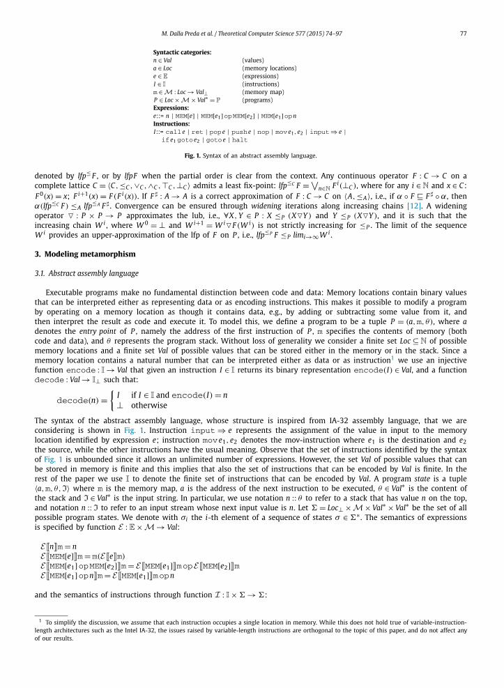
Syntactic categories:n ∈ Val (values)a ∈ Loc (memory locations)e ∈ E (expressions)I ∈ I (instructions)m ∈ M : Loc → Val⊥ (memory map)P ∈ Loc ×M× Val∗ = P (programs)Expressions:e::= n | MEM[e] | MEM[e1]opMEM[e2] | MEM[e1]opnInstructions:I::= call e | ret | pop e | push e | nop | mov e1, e2 | input⇒ e |if e1 goto e2 | goto e | halt
Fig. 1. Syntax of an abstract assembly language.
denoted by lfp≤ F , or by lfpF when the partial order is clear from the context. Any continuous operator F : C → C on a complete lattice C = 〈C, ≤C , ∨C , ∧C , �C , ⊥C 〉 admits a least fix-point: lfp≤C F = ∨
n∈N F i(⊥C ), where for any i ∈N and x ∈ C : F 0(x) = x; F i+1(x) = F (F i(x)). If F � : A → A is a correct approximation of F : C → C on 〈A, ≤A〉, i.e., if α ◦ F F � ◦ α, then α(lfp≤C F ) ≤A lfp≤A F � . Convergence can be ensured through widening iterations along increasing chains [12]. A widening operator � : P × P → P approximates the lub, i.e., ∀X, Y ∈ P : X ≤P (X�Y ) and Y ≤P (X�Y ), and it is such that the increasing chain W i , where W 0 = ⊥ and W i+1 = W i�F (W i) is not strictly increasing for ≤P . The limit of the sequence W i provides an upper-approximation of the lfp of F on P , i.e., lfp≤P F ≤P limi→∞W i .
3. Modeling metamorphism
3.1. Abstract assembly language
Executable programs make no fundamental distinction between code and data: Memory locations contain binary values that can be interpreted either as representing data or as encoding instructions. This makes it possible to modify a program by operating on a memory location as though it contains data, e.g., by adding or subtracting some value from it, and then interpret the result as code and execute it. To model this, we define a program to be a tuple P = (a, m, θ), where adenotes the entry point of P , namely the address of the first instruction of P , m specifies the contents of memory (both code and data), and θ represents the program stack. Without loss of generality we consider a finite set Loc ⊆ N of possible memory locations and a finite set Val of possible values that can be stored either in the memory or in the stack. Since a memory location contains a natural number that can be interpreted either as data or as instruction1 we use an injective function encode : I → Val that given an instruction I ∈ I returns its binary representation encode(I) ∈ Val, and a function decode : Val → I⊥ such that:
decode(n) ={
I if I ∈ I and encode(I) = n⊥ otherwise
The syntax of the abstract assembly language, whose structure is inspired from IA-32 assembly language, that we are considering is shown in Fig. 1. Instruction input ⇒ e represents the assignment of the value in input to the memory location identified by expression e; instruction mov e1, e2 denotes the mov-instruction where e1 is the destination and e2the source, while the other instructions have the usual meaning. Observe that the set of instructions identified by the syntax of Fig. 1 is unbounded since it allows an unlimited number of expressions. However, the set Val of possible values that can be stored in memory is finite and this implies that also the set of instructions that can be encoded by Val is finite. In the rest of the paper we use I to denote the finite set of instructions that can be encoded by Val. A program state is a tuple 〈a, m, θ, I〉 where m is the memory map, a is the address of the next instruction to be executed, θ ∈ Val∗ is the content of the stack and I ∈ Val∗ is the input string. In particular, we use notation n :: θ to refer to a stack that has value n on the top, and notation n :: I to refer to an input stream whose next input value is n. Let = Loc⊥ ×M × Val∗ × Val∗ be the set of all possible program states. We denote with σi the i-th element of a sequence of states σ ∈ ∗ . The semantics of expressions is specified by function E : E ×M → Val:
E�n�m = nE�MEM[e]�m = m(E�e�m)
E�MEM[e1] opMEM[e2]�m = E�MEM[e1]�m opE�MEM[e2]�mE�MEM[e1] opn�m = E�MEM[e1]�m opn
and the semantics of instructions through function I : I × → :
1 To simplify the discussion, we assume that each instruction occupies a single location in memory. While this does not hold true of variable-instruction-length architectures such as the Intel IA-32, the issues raised by variable-length instructions are orthogonal to the topic of this paper, and do not affect any of our results.
78 M. Dalla Preda et al. / Theoretical Computer Science 577 (2015) 74–97
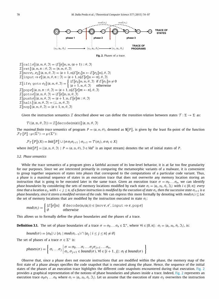
Fig. 2. Phases of a trace.
I�call e�〈a, m, θ, I〉 = 〈E�e�m, m, (a + 1) :: θ, I〉I�ret�〈a, m, n :: θ, I〉 = 〈n, m, θ, I〉I�mov e1, e2 �〈a, m, θ, I〉 = 〈a + 1, m[E�e1 �m ← E�e2 �m], θ, I〉I�input⇒ e�〈a, m, θ, n :: I〉 = 〈a + 1, m[E�e�m ← n], θ, I〉I�if e1 goto e2 �〈a, m, θ, I〉 =
{ 〈E�e2 �m,m, θ,I〉 if E�e1 �m �= 0〈a + 1,m, θ,I〉 otherwise
I�pop e�〈a, m, n :: θ, I〉 = 〈a + 1, m[E�e�m ← n], θ, I〉I�goto e�〈a, m, θ, I〉 = 〈E�e�m, m, θ, I〉I�push e�〈a, m, θ, I〉 = 〈a + 1, m, E�e�m :: θ, I〉I�halt�〈a, m, θ, I〉 = 〈⊥, m, θ, I〉I�nop�〈a, m, θ, I〉 = 〈a + 1, m, θ, I〉
Given the instruction semantics I described above we can define the transition relation between states T : → as:
T (〈a,m, θ,I〉) = I�decode(m(a))�〈a,m, θ,I〉The maximal finite trace semantics of program P = (a, m, θ), denoted as S� P �, is given by the least fix-point of the function FT � P � : ℘( ∗) → ℘( ∗):
FT � P �(X) = Init� P � ∪ {σσiσi+1 | σi+1 = T (σi),σσi ∈ X}where Init� P � = {〈a, m, θ, I〉 | P = (a, m, θ), I ∈ Val∗ is an input stream} denotes the set of initial states of P .
3.2. Phase semantics
While the trace semantics of a program gives a faithful account of its low-level behavior, it is at far too fine granularity for our purposes. Since we are interested primarily in comparing the metamorphic variants of a malware, it is convenient to group together sequences of states into phases that correspond to the computations of a particular code variant. Thus, a phase is a maximal sequence of states in an execution trace that does not overwrite any memory location storing an instruction that is going to be executed later in the same trace. Given an execution trace σ = σ0 . . . σn , we can identify phase boundaries by considering the sets of memory locations modified by each state σi = 〈ai, mi, θi, Ii〉 with i ∈ [0, n]: every time that a location a j , with i < j ≤ n, of a future instruction is modified by the execution of state σi , then the successive state σi+1 is a phase boundary, since it stores a modified version of the code. We can express this more formally by denoting with mod(σi) ⊆ Locthe set of memory locations that are modified by the instruction executed in state σi :
mod(σi) ={ {E�e�m} if decode(mi(ai)) ∈ {mov e, e′,input⇒ e,pop e}
∅ otherwise
This allows us to formally define the phase boundaries and the phases of a trace.
Definition 3.1. The set of phase boundaries of a trace σ = σ0 . . . σn ∈ ∗ , where ∀i ∈ [0, n] : σi = 〈ai, mi, θi, Ii〉, is:
bound(σ ) = {σ0} ∪ {σi | mod(σi−1) ∩ {a j | i ≤ j ≤ n} �= ∅}The set of phases of a trace σ ∈ ∗ is:
phases(σ ) ={
σi . . . σ j
∣∣∣∣ σ = σ0 . . . σi . . . σ jσ j+1 . . . σn,
σi,σ j+1 ∈ bound(σ ),∀l ∈ [i + 1, j] : σl /∈ bound(σ )
}
Observe that, since a phase does not execute instructions that are modified within the phase, the memory map of the first state of a phase always specifies the code snapshot that is executed along the phase. Hence, the sequence of the initial states of the phases of an execution trace highlights the different code snapshots encountered during that execution. Fig. 2provides a graphical representation of the notions of phase boundaries and phases inside a trace. Indeed, Fig. 2 represents an execution trace σ0σ1 . . . σ8 where σi = 〈ai, mi, θi, Ii〉. Let us assume that the execution of state σ2 overwrites the instruction
M. Dalla Preda et al. / Theoretical Computer Science 577 (2015) 74–97 79
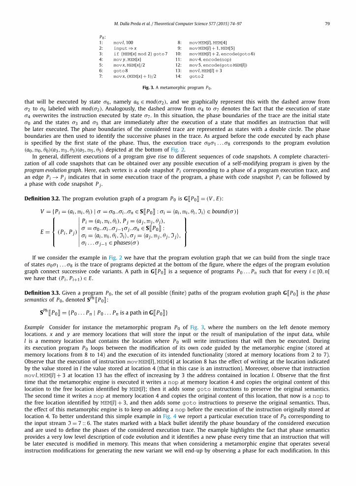
P0:1: mov l,100 8: movMEM[l],MEM[4]2: input⇒ x 9: movMEM[l] + 1,MEM[5]3: if (MEM[x] mod 2) goto7 10: movMEM[l] + 2,encode(goto6)
4: mov y,MEM[x] 11: mov4,encode(nop)
5: mov x,MEM[x]/2 12: mov5,encode(gotoMEM[l])6: goto8 13: mov l,MEM[l] + 37: mov x, (MEM[x] + 1)/2 14: goto2
Fig. 3. A metamorphic program P0.
that will be executed by state σ6, namely a6 ∈ mod(σ2), and we graphically represent this with the dashed arrow from σ2 to σ6 labeled with mod(σ2). Analogously, the dashed arrow from σ4 to σ7 denotes the fact that the execution of state σ4 overwrites the instruction executed by state σ7. In this situation, the phase boundaries of the trace are the initial state σ0 and the states σ3 and σ5 that are immediately after the execution of a state that modifies an instruction that will be later executed. The phase boundaries of the considered trace are represented as states with a double circle. The phase boundaries are then used to identify the successive phases in the trace. As argued before the code executed by each phase is specified by the first state of the phase. Thus, the execution trace σ0σ1 . . . σ8 corresponds to the program evolution (a0, m0, θ0)(a3, m3, θ3)(a5, m5, θ5) depicted at the bottom of Fig. 2.
In general, different executions of a program give rise to different sequences of code snapshots. A complete characteri-zation of all code snapshots that can be obtained over any possible execution of a self-modifying program is given by the program evolution graph. Here, each vertex is a code snapshot Pi corresponding to a phase of a program execution trace, and an edge Pi → P j indicates that in some execution trace of the program, a phase with code snapshot Pi can be followed by a phase with code snapshot P j .
Definition 3.2. The program evolution graph of a program P0 is G� P0 � = (V , E):
V = {Pi = (ai,mi, θi) | σ = σ0..σi ..σn ∈ S� P0 � : σi = 〈ai,mi, θi,Ii〉 ∈ bound(σ )}
E =
⎧⎪⎪⎨⎪⎪⎩
(Pi, P j)
∣∣∣∣∣∣∣∣
Pi = (ai,mi, θi), P j = (a j,m j, θ j),
σ = σ0..σi ..σ j−1σ j..σn ∈ S� P0 � :σi = 〈ai,mi, θi,Ii〉,σ j = 〈a j,m j, θ j,I j〉,σi . . . σ j−1 ∈ phases(σ )
⎫⎪⎪⎬⎪⎪⎭
If we consider the example in Fig. 2 we have that the program evolution graph that we can build from the single trace of states σ0σ1 . . . σ8 is the trace of programs depicted at the bottom of the figure, where the edges of the program evolution graph connect successive code variants. A path in G� P0 � is a sequence of programs P0 . . . Pn such that for every i ∈ [0, n[we have that (Pi, Pi+1) ∈ E .
Definition 3.3. Given a program P0, the set of all possible (finite) paths of the program evolution graph G� P0 � is the phase semantics of P0, denoted SPh � P0 �:
SPh � P0 � = {P0 . . . Pn | P0 . . . Pn is a path in G� P0 �}
Example Consider for instance the metamorphic program P0 of Fig. 3, where the numbers on the left denote memory locations. x and y are memory locations that will store the input or the result of manipulation of the input data, while l is a memory location that contains the location where P0 will write instructions that will then be executed. During its execution program P0 loops between the modification of its own code guided by the metamorphic engine (stored at memory locations from 8 to 14) and the execution of its intended functionality (stored at memory locations from 2 to 7). Observe that the execution of instruction movMEM[l], MEM[4] at location 8 has the effect of writing at the location indicated by the value stored in l the value stored at location 4 (that in this case is an instruction). Moreover, observe that instruction mov l, MEM[l] + 3 at location 13 has the effect of increasing by 3 the address contained in location l. Observe that the first time that the metamorphic engine is executed it writes a nop at memory location 4 and copies the original content of this location to the free location identified by MEM[l]; then it adds some goto instructions to preserve the original semantics. The second time it writes a nop at memory location 4 and copies the original content of this location, that now is a nop to the free location identified by MEM[l] + 3, and then adds some goto instructions to preserve the original semantics. Thus, the effect of this metamorphic engine is to keep on adding a nop before the execution of the instruction originally stored at location 4. To better understand this simple example in Fig. 4 we report a particular execution trace of P0 corresponding to the input stream I = 7 :: 6. The states marked with a black bullet identify the phase boundary of the considered execution and are used to define the phases of the considered execution trace. The example highlights the fact that phase semantics provides a very low level description of code evolution and it identifies a new phase every time that an instruction that will be later executed is modified in memory. This means that when considering a metamorphic engine that operates several instruction modifications for generating the new variant we will end-up by observing a phase for each modification. In this

80 M. Dalla Preda et al. / Theoretical Computer Science 577 (2015) 74–97
phase-1 • σ1 = 〈1,m1, θ,7 :: 6〉σ2 = 〈2,m2 = m1[l ← 100], θ,7 :: 6〉σ3 = 〈3,m3 = m2[x ← 7], θ,6〉σ4 = 〈7,m4 = m3, θ,6〉σ5 = 〈8,m5 = m4[x ← 4], θ,6〉
phase-2 • σ6 = 〈9,m6 = m2[100 ← encode(mov y,MEM[x])], θ,6〉phase-3 • σ7 = 〈10,m7 = m6[101 ← encode(mov x,MEM[x]/2)], θ,6〉phase-4 • σ8 = 〈11,m8 = m7[102 ← encode(goto6)], θ,6〉phase-5 • σ9 = 〈12,m9 = m8[4 ← encode(nop)], θ,6〉phase-6 • σ10 = 〈13,m10 = m9[5 ← encode(goto100)], θ,6〉
σ11 = 〈14,m11 = m10[l ← 103], θ,6〉σ12 = 〈2,m12 = m11, θ,6〉σ13 = 〈3,m13 = m12[x ← 6], θ, ε〉σ14 = 〈4,m14 = m13, θ, ε〉σ15 = 〈5,m15 = m14, θ, ε〉σ16 = 〈100,m16 = m14, θ, ε〉σ17 = 〈101,m17 = m16[y ← 6], θ, ε〉σ18 = 〈102,m18 = m17[x ← 3], θ, ε〉σ19 = 〈6,m19 = m18, θ, ε〉σ20 = 〈8,m20 = m19, θ, ε〉
phase-7 • σ21 = 〈9,m21 = m20[103 ← encode(nop)], θ, ε〉phase-8 • σ22 = 〈10,m22 = m21[104 ← encode(goto100)], θ, ε〉phase-9 • σ23 = 〈11,m23 = m22[105 ← encode(goto6)], θ, ε〉phase-10 • σ24 = 〈12,m24 = m23[4 ← encode(nop)], θ, ε〉phase-11 • σ25 = 〈13,m25 = m24[5 ← encode(goto103)], θ, ε〉
σ26 = 〈14,m26 = m25[l ← 106], θ, ε〉σ27 = 〈2,m27 = m26, θ, ε〉. . .
Fig. 4. Execution trace of P0 with input stream I= 7 :: 6.
cases it would be nice and useful to further abstract the model of phase semantics in order to observe only the “final” code variant obtained through this series of intermediate modifications. The formal definition of this abstraction will be based on some knowledge of the metamorphic engine that we are considering. In Section 7 we will provide an example of this when considering the metamorphic malware MetaPHOR.
3.3. Fix-point phase semantics
It is possible to define a function on 〈℘(P∗), ⊆〉 that iteratively computes the phase semantics of a given program. In order to do this we introduce the notion of mutating transition: A transition between two states that leads to a state which is a phase boundary.
Definition 3.4. We say that a pair of states (σi, σ j) is a mutating transition of P0, denoted (σi, σ j) ∈ MT(P0), if there exists a trace σ = σ0 . . . σiσ j . . . σn ∈ S� P0 � such that σ j ∈ bound(σ ).
From the above notion of mutating transition we can derive the program transformer T Ph : ℘(P) → ℘(P) that associates with each set of programs the set of their possible metamorphic variants, i.e., P j ∈ T Ph(Pi) means that, during execution, program Pi can be transformed into program P j .
Definition 3.5. The transition relation between programs T Ph : ℘(P) → ℘(P) is given by the point-wise extension of T Ph :P → ℘(P) where ∀P0 ∈ P:
T Ph(P0) ={
Pl
∣∣∣∣ Pl = (al,ml, θl),σ = σ0 . . . σl−1σl ∈ S� P0 �,σl = 〈al,ml, θl,Il〉,(σl−1,σl) ∈ MT(P0),∀i ∈ [0, l − 1[: (σi,σi+1) /∈ MT(P0)
}
and T Ph(P0) = ∅ if P0 is not self-modifying.
The transition relation T Ph can be extended to traces of programs by defining function FT Ph � P0 � : ℘(P∗) → ℘(P∗) as:
FT Ph � P0 �(Z) = P0 ∪ {zPi P i+1 | Pi+1 ∈ T Ph(Pi), zPi ∈ Z}The following lemma shows that FT � P0 � and FT Ph � P0 � are extensive functions when considering prefix ordering on strings.
M. Dalla Preda et al. / Theoretical Computer Science 577 (2015) 74–97 81
Lemma 3.6. The following implications hold:
(1) If P0 . . . Pl Pl+1 ∈FT Ph � P0 �(Z) then P0 . . . Pl ∈ Z and Pl+1 ∈ T Ph(Pl).(2) If σ0 . . . σnσn+1 ∈FT � P �(X) then σ0 . . . σn ∈ X and σn+1 ∈ T (σn).(3) If σ0 . . . σl . . . σn ∈ S� P0 �, where σ0 = 〈a0, m0, θ0, I0〉, σl = 〈al, ml, θl, Il〉, P0 = (a0, m0, θ0) and Pl = (al, ml, θl), then σl . . . σn ∈
S� Pl �.
Proof. Immediate by definition of FT Ph � P0 �, FT � P0 � and S� P �. �The following result shows how function FT Ph � P0 � iteratively computes the phase semantics of P0.
Theorem 3.7. lfp⊆FT Ph � P0 � = SPh � P0 �.
Proof. In the rest of the proof we consider that ∀i ∈ N: σi = 〈ai, mi, θi, Ii〉 and Pi = (ai, mi, θi). Let us show that SPh � P0 � ⊆ lfp⊆FT Ph � P0 �. We prove this by showing by induction on the length of the string that ∀z ∈ P
∗ : z ∈ SPh � P0 � ⇒z ∈ lfp⊆FT Ph � P0 �. The only path of length one in G� P0 � is P0, and the only string of length one in lfp⊆FT Ph � P0 � is P0. Assume that the above implication holds for every string of length n and let us show that it holds for z = P0 . . . Pl Pkof length n + 1. If P0 . . . Pl Pk is a path of G� P0 � = (V , E) it means that P0 . . . Pl is a path of G� P0 � = (V , E) and that (Pl, Pk) ∈ E . By Definition 3.2 of program evolution graph, this means that P0 . . . Pl is a path of G� P0 � and that there exists σ = σ0 . . . σl−1σl . . . σk−1σk . . . σn ∈ S� P0 � such that σl . . . σk−1 ∈ phases(σ ). By Definition 3.1 of phases this means that {σl, σk} ⊆ bound(σ ) and ∀i ∈ ]l, k − 1] : σi /∈ bound(σ ). By induction hypothesis and by point (3) of Lemma 3.6 we have that P0 . . . Pl ∈ lfp⊆FT Ph � P0 � and that ∃σ ′ = σl . . . σk−1σk . . . σn ∈ S� Pl � such that σk ∈ bound(σ ′)and ∀i ∈ ]l, k − 1] : σi /∈ bound(σ ′). By Definition 3.4 of mutating transition this implies that (σk−1, σk) ∈ MT(Pl) and ∀i ∈ [l, k − 1[: (σi, σi+1) /∈ MT(Pl). By Definition 3.5 of T Ph this means that Pk ∈ T Ph(Pl). From which we can conclude that, P0 . . . Pl Pk ∈ lfp⊆FT Ph � P0 �.
Let us now show that lfp⊆FT Ph � P0 � ⊆ SPh � P0 �. We prove this by showing that ∀z ∈ P∗ : z ∈ lfp⊆FT Ph � P0 � ⇒ z ∈
SPh � P0 �. Consider P0 . . . Pl Pl+1 ∈ lfp⊆FT Ph � P0 �. This means that ∀i ∈ [0, l] : Pi+1 ∈ T Ph(Pi). By Definition 3.5 of T Ph , we have that ∀i ∈ [0, l], there exists ni ∈ N such that σ i = σiσi1 . . . σini
σi+1 ∈ S� Pi � such that (σini, σi+1) ∈ MT(Pi),
∀k ∈ [1, ni[: (σik , σik+1) /∈ MT(Pi), and (σi, σi1 ) /∈ MT(Pi). By concatenating all the traces connecting pairs of programs in transition relation we obtain a trace σ = σ 0σ 1 . . . σ l = σ0σ01 . . . σ0n0
σ1 . . . σlnlσl+1 ∈ S� P0 � such that ∀i ∈ [0, l + 1] : σi ∈
bound(σ ) ∧ ∀k ∈ [1, ni] : σik /∈ bound(σ ). By Definition 3.1 this means that ∀i ∈ [0, l] : σiσi1 . . . σini∈ phases(σ ). By Defini-
tion 3.2 of program evolution graph, this means that ∀i ∈ [0, l] : (Pi, Pi+1) ∈ E , which implies that P0 . . . Pl Pl+1 ∈ SPh � P0 �and concludes the proof. �3.4. Correctness and completeness of phase semantics
We prove the correctness of phase semantics by showing that it is a sound approximation of maximal finite trace semantics, namely by providing a pair of adjoint maps αPh : ℘( ∗) → ℘(P∗) and γPh : ℘(P∗) → ℘( ∗), for which the fix-point computation of FT Ph � P0 � approximates the fix-point computation of FT � P0 �. Given a trace σ =〈a0, m0, θ0, I0〉 . . . σi−1σi . . . σn we define the abstraction function αPh as αPh(σ ) = (a0, m0, θ0)αPh(σi . . . σn) such that σi ∈bound(σ ) and ∀l ∈ [0, i − 1] : σl /∈ bound(σ ), while α(ε) = ε . The idea is that abstraction αPh observes only the states of a trace that are phase boundaries and it can be lifted point-wise to ℘( ∗) giving rise to the Galois connection (℘ ( ∗), αPh, γPh, ℘(P∗)). The following result shows that the fix-point computation of phase semantics approximates the fix-point computation of trace semantics, thus proving that phase semantics is a sound abstraction of trace semantics on the abstract domain ℘(P∗).
Theorem 3.8. ∀X ∈ ℘( ∗) αPh(X ∪FT � P0 �(X)) ⊆ αPh(X) ∪FT Ph � P0 �(αPh(X)).
Proof. Let us consider P0 . . . Pl Pk ∈ αPh(X ∪ FT � P0 �(X)). Function αPh is additive, i.e., αPh(X ∪ FT � P0 �(X)) = αPh(X) ∪αPh(FT � P0 �(X)), and we can therefore distinguish the two following cases:
(1): P0 . . . Pl Pk ∈ αPh(X) which immediately implies that the program sequence P0 . . . Pl Pk ∈ αPh(X) ∪FT Ph � P0 �(αPh(X)).(2): P0 . . . Pl Pk ∈ αPh(FT � P0 �(X)). In this case we have that there exists σσiσ j ∈ FT � P0 �(X) such that αPh(σσiσ j) =
P0 . . . Pl Pk . By point (2) of Lemma 3.6, this means that ∃σσi ∈ X such that σ j = T (σi), and αPh(σσiσ j) = P0 . . . Pl Pk . We have two possible cases:
(A) αPh(σσi) = P0 . . . Pl Pk , which means that P0 . . . Pl Pk ∈ αPh(X) and therefore we are back to case (1).(B) αPh(σσi) = P0 . . . Pl and αPh(σσiσ j) = P0 . . . Pl Pk . This means that P0 . . . Pl ∈ αPh(X) and, by following the defini-
tion of αPh and point (3) of Lemma 3.6, that σσiσ j = σ0 . . . σl . . . σiσ j ∈ FT � P0 �(X) is such that σ ′ = σl . . . σiσ j ∈ S� Pl �and σ j ∈ bound(σ ′) and ∀ f ∈ [l + 1, i] : σ f /∈ bound(σ ′). This means that P0 . . . Pl ∈ αPh(X) and σ ′ = σl . . . σiσ j ∈ S� Pl �
is such that (σi, σ j) ∈ MT(Pl) and σ j = 〈ak, mk, θk, Ik〉 and ∀ f ∈ [l, i[: (σ f , σ f +1) /∈ MT(Pl). By Definition 3.5 of T Ph , this
82 M. Dalla Preda et al. / Theoretical Computer Science 577 (2015) 74–97
means that P0 . . . Pl ∈ αPh(X) and Pk ∈ T Ph(Pl), where Pk = (ak, mk, θk). From this we can conclude that P0 . . . Pl Pk ∈FT Ph � P0 �(αPh(X)). �
Observe that, in general, the converse of the theorem above may not hold, namely we may have that αPh(X ∪FT � P0 �(X)) ⊂ αPh(X) ∪FT Ph � P0 �(αPh(X)). In fact, given X ∈ ℘( ∗), the concrete function FT � P0 � makes only one tran-sition in T and this may not be a mutating transition, while the abstract function FT Ph � P0 � “jumps” directly to the next mutating transition. Even if the fix-point computation of FT Ph � P0 � is not step-wise complete [24], it is complete at the fix-point, as shown by the following theorem, proving completeness of the phase semantics.
Theorem 3.9. αPh(lfp⊆FT � P0 �) = lfp⊆FT Ph � P0 �.
Proof. For readability in the proof we omit the apex denoting the partial order on which the lfp is computed. In the rest of the proof we consider that for every i ∈N: σi = 〈ai, mi, θi, Ii〉 and Pi = (ai, mi, θi).
Let us show that αPh(lfpFT � P0 �) ⊆ lfpFT Ph � P0 �. We prove this by showing by induction on the length of the string that ∀z ∈ P
∗ : z ∈ αPh(lfpFT � P0 �) ⇒ z ∈ lfpFT Ph � P0 �. By definition we have that the only string of length 1 that belongs to αPh(lfpFT � P0 �) is P0, and the only string of length 1 that belongs to lfpFT Ph � P0 � is P0. Assume that the above implication holds for any string of length n and consider the string P0 . . . Pl Pk of length n + 1. If P0 . . . Pl Pk ∈ αPh(lfpFT � P0 �) it means that ∃σ = σ0 . . . σl . . . σk−1σk ∈ lfpFT � P0 � such that αPh(σ ) = P0 . . . Pl Pk , namely that ∃σ = σ0 . . . σl . . . σk−1σk ∈ S� P0 � such that αPh(σ ) = P0 . . . Pl Pk . By induction and by following the definition of αPh and point (3) of Lemma 3.6, we have that P0 . . . Pl ∈ lfpFT Ph � P0 � and ∃σ ′ = σl . . . σk−1σk ∈ S� Pl � such that σk ∈ bound(σ ′) and ∀i ∈ [l + 1, k − 1] : σi /∈ bound(σ ′). This means that (σk−1, σk) ∈ MT(Pl) and ∀i ∈ [l, k − 1[: (σi, σi+1) /∈ MT(Pl). By Definition 3.5 of T Ph we have that Pk ∈ T Ph(Pl), from which we can conclude that P0 . . . Pl Pk ∈ lfpFT Ph � P0 �.
Let us show that lfpFT Ph � P0 � ⊆ αPh(lfpFT � P0 �). We prove this by showing by induction on the length of the strings that ∀z ∈ P
∗ : z ∈ lfpFT Ph � P0 � ⇒ z ∈ αPh(lfpFT � P0 �). For the strings of length 1 we have the same argument as before. Assume that the above implication holds for every string of length n and consider P0 . . . Pl Pk of length n + 1. Assume that P0 . . . Pl Pl+1 ∈ lfpFT Ph � P0 �. From point (1) of Lemma 3.6 this means that P0 . . . Pl ∈ lfpFT Ph � P0 � and Pl+1 ∈ T Ph(Pl). By induction and from Definition 3.5 of T Ph we have that P0 . . . Pl ∈ αPh(lfpFT � P0 �) and ∃σ l = σlσl1 . . . σlnlσl+1 ∈ S� Pl �such that (σlnl
, σl+1) ∈ MT(Pl) and ∀i ∈ [l, l[: (σli , σli+1 ) /∈ MT(Pl) and (σl, σ l1) /∈ MT(Pl). This means that ∃σ0 . . . σl ∈lfpFT � P0 � such that αPh(σ0 . . . σl) = P0 . . . Pl . This implies that there exists a trace σ0 . . . σl . . . σl+1 ∈ lfpFT � P0 � such that αPh(σ0 . . . σl . . . σl+1) = P0 . . . Pl Pl+1 and therefore that P0 . . . Pl Pl+1 ∈ αPh(lfpFT � P0 �). �4. Abstracting metamorphism
Consider a sequence P0 P1 P2 . . . ∈ SPh � P0 � in the phase semantics of a metamorphic program P0. By definition this means that during execution the program P0 may evolve into the syntactically different but semantically equivalent pro-gram P1, then into program P2 and so on. Thus, a program Q is a metamorphic variant of a program P0, denoted P0 �Ph Q , if Q is an element of at least one trace in SPh � P0 �. This leads to the following concrete test for metamorphism:
P0 �Ph Q ⇔ ∃P0 P1 . . . Pn ∈ SPh � P0 �,∃i ∈ [0,n] : Pi = Q (1)
Thanks to the completeness of phase semantics, the above concrete test for metamorphic variant avoids both false positives and false negatives. Unfortunately, the phase semantics of a metamorphic program may present infinite traces, modeling infinite code evolutions, and this means that it may not be possible to decide whether a program appears (or not) in the phase semantics of a metamorphic program. So phase semantics provides a very precise model of code evolution that leads to a test for metamorphism that is undecidable in general. In order to gain decidability we have to loose precision. In particular, our idea is to abstract the phase semantics in order to obtain an approximated model of code evolution that leads to a decidable abstract test for metamorphism. Indeed, the considered model of metamorphic code behavior is based on a very low-level representation of programs as memory maps that simply give the contents of memory locations together with the address of the instruction to be executed next. While such a representation is necessary to precisely capture the effects of code self-modification, it is not a convenient representation if we want to statically recognize the different code snapshots encountered during a program’s execution. Instead, we would like to consider a suitable abstraction of the domain of programs where it is possible to compute an approximation of the metamorphic behavior of a self-modifying program that can be used to decide whether a program is a metamorphic variant of another one. The idea is to determine an abstract interpretation of phase semantics, namely to approximate the computation of phase semantics on an abstract domain that captures properties of the evolution of the code, rather than of the evolution of program states, as usual in abstract interpretation. Following the standard abstract interpretation approach to static program analysis [12], we have to:
• Define an abstract domain 〈A, A〉 of code properties that gives rise to a Galois connection (℘ (P∗), αA, γA, A);• Define the abstract transition relation T A : ℘(A) → ℘(A) and the abstract function FT A � P0 � : A → A such that
lfp AFT A � P0 � = SA � P0 � provides an abstract specification of the metamorphic behavior on A;

M. Dalla Preda et al. / Theoretical Computer Science 577 (2015) 74–97 83
• Prove that SA � P0 � is a correct approximation of phase semantics SPh � P0 �, namely that αA(lfp⊆FT Ph � P0 �) Alfp AFT A � P0 �.
The abstract specification SA � P0 �, obtained as abstract interpretation of the phase semantics, induces an abstract notion of metamorphic variant with respect to the abstract domain A: A program Q is a metamorphic variant of program P0 with respect to the abstract domain A, denoted P0 �A Q , if SA � P0 � approximates Q in the abstract domain A. This leads to the following abstract test for metamorphism wrt A:
P0 �A Q ⇔ αA(Q ) A SA � P0 �
In this sense, SA � P0 � is an abstract metamorphic signature for P0. Whenever SA � P0 � is a correct approximation of phase semantics, we have that P0 �A Q avoids false negatives, namely the abstract metamorphic test never misses a program that is a metamorphic variant of P0. The absence of false positives is not guaranteed in general and it may need a refinement of the abstract domain A [24]. In fact, due to the loss of precision of the abstraction process it may happen that the above test on the abstract metamorphic signature classifies a program as a metamorphic variant of the original malware P0 even if it is not. For example, if we consider the most abstract domain A = {�} that maps every program and every phase semantics in � we would have an abstract test for metamorphism that says that every program is a metamorphic variant of another one. Of course this result is sound in the sense that we have no false negatives, while it is very imprecise since we have the maximal amount of false positives. Indeed, there is a wide gamma of abstract domains between the concrete domain of programs (used to compute the precise phase semantics) and the abstract domain A = {�}, and we have to carefully choose the abstract domain in order to gain decidability while keeping a good degree of precision. How to choose this abstract domains is a challenging task. Of course the decidability of the abstract test for metamorphism depends on the choice of the abstract domain A. The example at the end of Section 6 shows another case of loss of precision due to abstraction.
Observe that we are interested in abstract domains representing code properties, namely in abstract domains that need to approximate properties of sequences of instructions. This is an unusual view of abstract domains, which are instead tra-ditionally designed to approximate properties of the states computed by the program. Abstractions for approximating code properties can be achieved naturally by grammar-based, constraint-based and finite state automata abstractions [14]. This allows us to extract, by abstract interpretation, invariant properties of the code evolution in metamorphic code without any a priori knowledge about the obfuscations implemented in the metamorphic engine. This idea will be exploited in the fol-lowing section, where we propose to abstract each phase by an FSA, describing the sequence of instructions (or approximate descriptions of instructions) that may be disassembled from the corresponding memory. Of course intermediate abstractions can be considered in case we have some partial knowledge on the structure of possible obfuscations implemented by the metamorphic engine. As observed in [16], the knowledge of some aspects of the obfuscation implemented by the meta-morphic engine may induce an abstraction on traces which can be composed with the Galois connection identified by the adjoint maps αPh and γPh in order to provide a more abstract basic representation of phases, on which checking whether P0 �A Q is simpler.
5. Phase semantics as sequences of FSA
5.1. Phases as FSA
We introduce a representation of programs, where a program is specified by the sequences of possibly abstract instruc-tions that may occur during its execution. Traditionally, the most commonly used program representation that expresses the possible control flow behaviors of a program, and hence the possible instruction sequences that may be obtained from its execution, is the control flow graph. In this representation, the vertices contain the instructions to be executed, and the edges represent possible control flow. For our purposes, it is convenient to consider a dual representation where vertices corre-spond to program locations and abstract instructions label edges. The resulting representation, which is clearly isomorphic to standard control flow graphs up-to memory locations, is an FSA over an alphabet of instructions. The instructions that define the alphabet of the FSA associated with a phase could be a simplification of ordinary IA-32 instructions, later called abstract instructions. Let M P denote the FSA-representation of a given program P and let L(M P ) be the language it recog-nizes. The idea is that for each sequence in L(M P ) the order of the abstract instructions in the sequence corresponds to the execution order of the corresponding concrete instructions in at least one run of the control flow graph of P . Instructions are abstracted in order to provide a simplified alphabet and to be independent from low-level details that are not relevant when describing the malware metamorphic behaviour. Our construction is parametric in the instruction abstraction. In the rest of the paper, as a possible abstraction of instructions, we consider function ι : I → I defined as follows:
ι(I) = I =
⎧⎪⎪⎨⎪⎪⎩
call if I = call ee1 if I = if e1 goto e2goto if I = goto eI otherwise
Observe that since I is finite also the set I of abstract instructions is finite. The intuition beyond abstraction ι is to have a program representation that is independent from the particular memory locations used to store instructions, and this is
84 M. Dalla Preda et al. / Theoretical Computer Science 577 (2015) 74–97
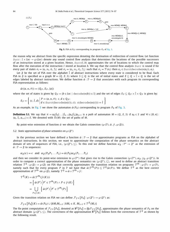
Fig. 5. FSA α(P0) corresponding to program P0 of Fig. 3.
the reason why we abstract from the specific expression denoting the destination of redirection of control flow. Let function Succ : I × Loc → ℘(Loc) denote any sound control flow analysis that determines the locations of the possible successors of an instruction stored at a given location. Hence, Succ(I, b) approximates the set of locations to which the control may flow after the execution of the instruction I stored at location b. We say that the control flow analysis Succ is sound if for every pair of states σi = 〈ai, mi, θi, Ii〉 and σ j = 〈a j, m j, θ j, I j〉 such that σ j = T (σi) then a j ∈ Succ(decode(m(ai)), ai).
Let F be the set of FSA over the alphabet I of abstract instructions where every state is considered to be final. Each FSA in F is specified as a graph M = (Q , E, S) where S ⊆ Q is the set of initial states and E ⊆ Q × I × Q is the set of edges labeled by abstract instructions. We define function α : P → F that associates with each program its corresponding FSA-representation as follows:
α((a,m, θ)) = (Q P , E P , {a})where the set of states is given by Q P = {b ∈ Loc | decode(m(b)) ∈ I} and the set of edges E P ⊆ Q P × I× Q P is given by:
E P ={
(c, I,d)
∣∣∣∣ P = (a,m, θ); c,d ∈ Q P ;d ∈ Succ(decode(m(c)), c); ι(decode(m(c))) = I
}
As an example, in Fig. 5 we show the automaton α(P0) corresponding to program P0 of Fig. 3.
Definition 5.1. We say that π = a0[ I0] . . . [ In−1]an[ In]an+1 is a path of automaton M = (Q , E, S) if a0 ∈ S and ∀i ∈ [0, n] :(ai, Ii, ai+1) ∈ E . We denoted with �(M) the set of paths of M .
By point-wise extension of function α we obtain the Galois connection (℘ (P), α, γ , ℘(F)).
5.2. Static approximation of phase semantics on ℘(F∗)
In the previous section we have defined a function α : P → F that approximates programs as FSA on the alphabet of abstract instructions. In this section, we want to approximate the computation of the phase semantics on the abstract domain of sets of sequences of FSA, i.e., 〈℘(F∗), ⊆〉. To this end we define function αF : P∗ → F∗ as the extension of α : P → F to sequences:
αF(ε) = ε and αF(P0 P1 . . . Pn) = α(P0)αF(P1 . . . Pn)
and then we consider its point-wise extension to ℘(P∗) that gives rise to the Galois connection (℘ (P∗), αF, γF, ℘(F∗)). In order to compute a correct approximation of the phase semantics on 〈℘(F∗), ⊆〉, we need to define an abstract transition relation T F : ℘(F) → ℘(F) on FSA that correctly approximates the transition relation on programs T Ph : ℘(P) → ℘(P), namely such that for every program P in P we have that α(T Ph(P )) ⊆ T F(α(P )). We define T F as the best correct approximation of T Ph on ℘(F), namely T F = α ◦ T Ph ◦ γ :
T F(K ) = α(T Ph(γ (K )))
={
α(P ′)∣∣∣P ′ ∈ T Ph(P ) ∧ P ∈ γ (K )
}
=⋃
P∈γ (K )
{α(P ′)
∣∣∣P ′ ∈ T Ph(P )}
Given the transition relation on FSA we can define FT F � P0 � : ℘(F∗) → ℘(F∗) as:
FT F � P0 �(K ) = α(P0) ∪ {kMi Mi+1 | kMi ∈ K , Mi+1 ∈ T F(Mi)}The fix-point computation of FT F � P0 �, denoted as SF� P0 � = lfpFT F � P0 �, approximates the phase semantics of P0 on the abstract domain 〈℘(F∗), ⊆〉. The correctness of the approximation SF� P0 � follows form the correctness of T F as shown by the following result.
M. Dalla Preda et al. / Theoretical Computer Science 577 (2015) 74–97 85
Theorem 5.2. αF(lfpFT Ph � P0 �) ⊆ lfpFT F � P0 � = SF� P0 �.
Proof. Let us prove that ω ∈ αF(lfpFT Ph � P0 �) ⇒ ω ∈ lfpFT F � P0 �. Let M0 . . . Mn ∈ αF(lfpFT Ph � P0 �), this means that ∃P0 . . . Pn ∈ lfpFT Ph � P0 � such that αF(P0 . . . Pn) = M0 . . . Mn . This means that ∀i ∈ [0, n[: Pi+1 ∈ T Ph(Pi) and ∀ j ∈ [1, n] :α(P j) = M j . From the correctness of T F we have that ∀P ∈ P : α(T Ph(P )) ⊆ T F(α(P )) and therefore: ∀i ∈ [0, n[: α(Pi+1) ∈T F(α(Pi)) and ∀ j ∈ [0, n] : α(P j) = M j . And this means that M0 . . . Mn ∈ lfpFT F � P0 �. �
SF� P0 � approximates the phase semantics of program P0 on 〈℘(F∗), ⊆〉 by abstracting programs with FSA, while the transitions, i.e., the metamorphic engine, follow directly from T Ph and are not approximated. For this reason SF� P0 � may still have infinite traces of FSAs thus leading to an abstract test of metamorphism that is still undecidable in general. In the following we introduce a static computable approximation of the transition relation on FSA that allows us to obtain a static approximation S�� P0 � of the phase semantics of P0 on 〈℘(F∗), ⊆〉. S�� P0 � may play the role of abstract metamorphic signature of P0. To this end, we introduce the notion of limits of a path that approximates the notion of bounds of a trace, and the notion of transition edge that approximates the notion of mutating transition. Moreover, we assume to have access to the following sound program analyses:
• a stack analysis StackVal : Loc → ℘(Val) that approximates the set of possible values on the top of the stack when control reaches a given location (e.g. [3,4]);
• a memory analysis LocVal : Loc × Loc → ℘(Val) that approximates the set of possible values that can be stored in a memory location when the control reaches a given location (e.g. [3,4]).
These analyses allow us to define the function EVal : Loc × E → ℘(Val), that approximates the evaluation of an expression in a given point:
EVal(b, n) = {n}EVal(b, MEM[e]) = {LocVal(b, l) | l ∈ EVal(b, e)}EVal(b, MEM[e1] opMEM[e2]) = {n1 opn2 | i ∈ {1, 2} : ni ∈ EVal(b, MEM[ei])}EVal(b, MEM[e] opn) = {n1 opn | n1 ∈ EVal(b, MEM[e])}
and a sound control flow analysis Succ : I × Loc → ℘(Loc):
Succ(I,b) =
⎧⎪⎪⎪⎨⎪⎪⎪⎩
EVal(b, e) if I ∈ {call e,goto e}StackVal(b) if I = ret{b + 1} ∪ EVal(b, e2) if I = if e1 goto e2,
∅ if I = halt{b + 1} otherwise
Moreover, function EVal allows us to define function write : I× Loc → ℘(Loc) that approximates the set of memory locations that may be modified by the execution of an abstract instruction stored at a given location:
write( I,b) ={
EVal(b, e) if I ∈ {mov e, e′,input⇒ e,pop e}∅ otherwise
With these assumptions, we define the limits of an execution path π as the nodes that are reached by an edge labeled by an abstract instruction that may modify the label of a future edge in π , namely an abstract instruction that occurs later in the same path. Given a path π = a0[ I0] . . . [ In−1]an we have:
limit(π) = {a0} ∪ {ai | write( I i−1,ai−1) ∩ {a j | i ≤ j ≤ n} �= ∅}
Definition 5.3. Consider an automata M = (Q , E, S) that represents a program. A pair of program locations (b, c) is a transition edge of M = (Q , E, S), denoted (b, c) ∈ TE(M), if there exists a ∈ S and an execution path π ∈ �(M) such that π = a[ Ia] . . . [ Ib−1]b[ Ib]c and c ∈ limit(π).
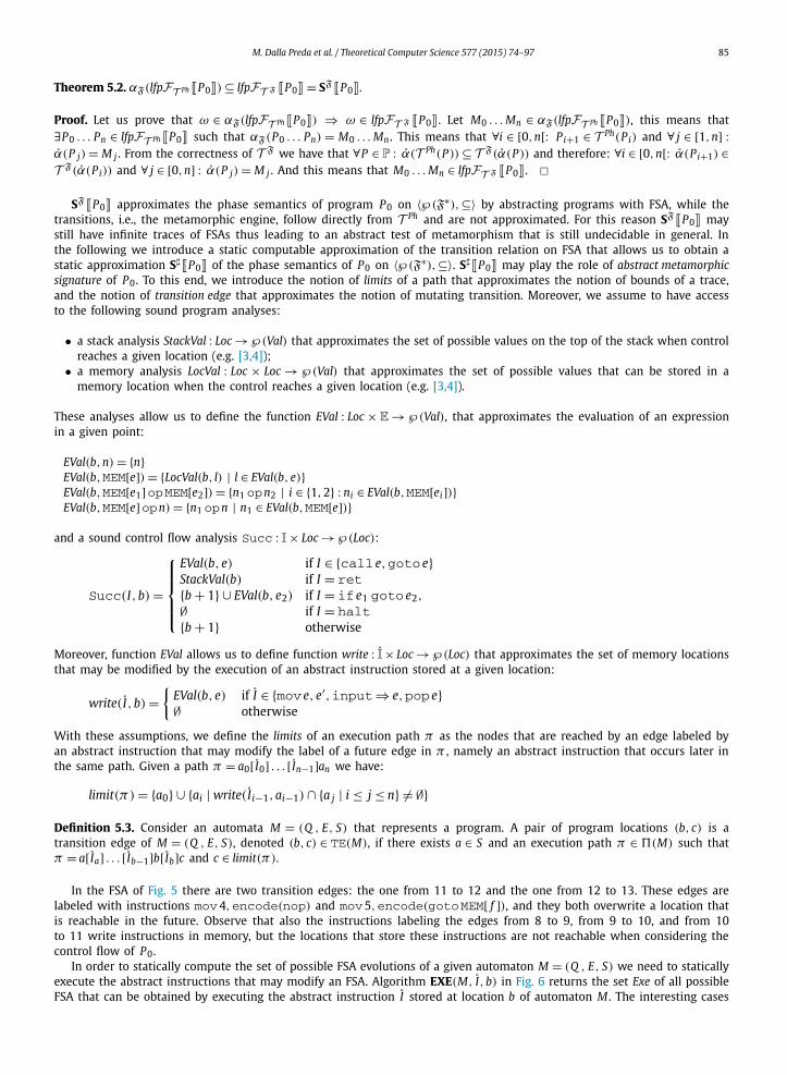
In the FSA of Fig. 5 there are two transition edges: the one from 11 to 12 and the one from 12 to 13. These edges are labeled with instructions mov4, encode(nop) and mov5, encode(gotoMEM[ f ]), and they both overwrite a location that is reachable in the future. Observe that also the instructions labeling the edges from 8 to 9, from 9 to 10, and from 10to 11 write instructions in memory, but the locations that store these instructions are not reachable when considering the control flow of P0.
In order to statically compute the set of possible FSA evolutions of a given automaton M = (Q , E, S) we need to statically execute the abstract instructions that may modify an FSA. Algorithm EXE(M, I, b) in Fig. 6 returns the set Exe of all possible FSA that can be obtained by executing the abstract instruction I stored at location b of automaton M . The interesting cases

86 M. Dalla Preda et al. / Theoretical Computer Science 577 (2015) 74–97
EXE(M, I,b) // M = (Q , E, S) is an FSAExe = {M ′ = (Q , E, S ′) | S ′ = {d | (b, I,d) ∈ E}}if I = mov e1, e2
then X = write( I,b)
Y = {n | n ∈ EVal(b, e2),decode(n) ∈ I}Exe = Exe ∪ NEXT(X, Y , M,b)
if I = input⇒ ethen X = write( I,b)
Y = {n | n is an input ,decode(n) ∈ I}Exe = Exe ∪ NEXT(X, Y , M,b)
if I = pop ethen X = write( I,b)
Y = {n | n ∈ StackVal(b),decode(n) ∈ I}Exe = Exe ∪ NEXT(X, Y , M,b)
return Exe
NEXT(X, Y , M,b)
Next = ∅for each a j ∈ X do
E = E � {(a j , I j , c) | (a j , I j , c) ∈ E}
Next = Next ∪ ⋃n∈Y
⎧⎨⎩ M = (Q , E, S)
∣∣∣∣∣∣Q = Q ∪ {a j} ∪ Succ(decode(n),a j)
E = E ∪ {(a j , ι(decode(n)),d) | d ∈ Succ(decode(n),a j)}S = {d | (b, I,d) ∈ E}
⎫⎬⎭
return Next
Fig. 6. Algorithm for statically executing instruction I .
of the algorithm are I = mov e1, e2, I = input⇒ e and I = pop e, since these are the only cases in which we might have a modification of the automaton.
The algorithm starts by initializing Exe to the FSA M ′ that has the same states and edges of M and whose possible initial states S ′ are the nodes reachable through the abstract instruction I stored at b in M . This ensures correctness when the execution of the abstract instruction I does not correspond to a real code mutation. Then if I writes in memory, namely if I ∈ {mov e1, e2, input ⇒ e, pop e}, we consider the set X of locations that can be modified by the execution of I , i.e., X = write( I, b), and the set Y of possible instructions that can be written by I in a location of X . Next, we add to Exe the set NEXT(X, Y , M, b) of all possible automata that can be obtained by writing an instruction of Y in a memory location in X . In particular, NEXT(X, Y , M, b) is based on the following observation: For each location a j in X and for each n ∈ Y we have an automaton M = (Q , E, S) to add to Exe where Q is obtained by adding to Q the location a j and the possible successors of the new instruction written by I at location a j ; E is obtained from E by deleting all the edges that start from a j (if any), and by adding for each n ∈ Y the edges {(a j, ιk(decode(n)), d) | d ∈ Succ(decode(n), a j)}, S is given by the set of nodes reachable through I in the original automaton M .
Let Evol(M) denote the possible evolutions of automaton M , namely the automata that can be obtained by the execution of the abstract instruction labeling the first transition edge of a path of M:
Evol(M) ={
M ′∣∣∣∣ a0[ I0] . . . [ Il−1]al[ Il]al+1 ∈ �(M), (al,al+1) ∈ TE(M),
∀i ∈ [0, l[: (ai,ai+1) /∈ TE(M), M ′ ∈ EXE(M, Il,al)
}
We can now define the static transition T � : ℘(F) → ℘(F). The idea is that the possible static successors of an automaton M are all the automata in Evol(M) together with all the automata M ′ that are different from M and that can be reached from M through a sequence of successive automata that differ from M only in the entry point. This ensures the correctness of T � , i.e., Ml ∈ T F(M0) ⇒ Ml ∈ T �(M0), even if between M0 and Ml there are spurious transition edges, i.e., transition edges that do not correspond to any mutating transition.
Definition 5.4. Let M = (Q , E, S). T � : ℘(F) → ℘(F) is given by the point-wise extension of:
T �(M) = Evol(M) ∪⎧⎨⎩ M ′
∣∣∣∣∣∣MM1 . . . Mk M ′ : M1 ∈ Evol(M),∀i ∈ [1,k[:Mi+1 ∈ Evol(Mi), M ′ = (Q ′, E ′, S ′) ∈ Evol(Mk),
(E �= E ′ ∨ Q �= Q ′),∀ j ∈ [1,k] : M j = (Q , E, S j)
⎫⎬⎭
Observe that X ⊆ Loc and Y ⊆ Val are finite sets and this ensures that the set of automata returned by the algorithm EXE(M, I, b) is finite and therefore the set of possible successors of any given automata M is finite. The following result shows that T � correctly approximates T F .
Lemma 5.5. For any M ∈ F : T F(M) ⊆ T �(M).
Proof. Let Ml ∈ T F(M0). By definition of T F this means Ml ∈ α(T Ph(γ (M0))). Which means that ∃P0 = (a0, m0, θ0), Pl = (al, ml, θl) : α(P0) = M0 and α(Pl) = Ml such that Pl ∈ T Ph(P0). By definition of T Ph this means that there exists
M. Dalla Preda et al. / Theoretical Computer Science 577 (2015) 74–97 87
P0 = (a0, m0, θ0), Pl = (al, ml, θl) : α(P0) = M0 and α(Pl) = Ml such that M0 = (Q 0, E0, S0), Ml = (Q l, El, Sl) and E0 �=El ∨ Q 0 �= Q l , moreover there exists σ0 . . . σl−1σl ∈ S� P0 � where (σl−1, σl) ∈ MT(P0) and ∀i ∈ [0, l − 2] : (σi, σi+1) /∈ MT(P0)
with ∀i ∈ [0, l] : σi = 〈ai, mi, θi, Ii〉. Thanks to the soundness of the analyses this means that: ∃P0 = (a0, m0, θ0), Pl =(al, ml, θl) : α(P0) = M0 and α(Pl) = Ml such that M0 = (Q 0, E0, S0), Ml = (Q l, El, Sl) and E0 �= El ∨ Q 0 �= Q l; moreover
there exists π = a0I0−→ . . .
Il−2−→ al−1Il−1−→ al ∈ �(M0) where ∀i ∈ [0, l[: ι(decode(mi(ai))) = I i and (al−1, al) ∈ TE(M0). Here
we have two possible cases:
(1) ∀ j ∈ [0, l − 2] : (a j, a j+1) /∈ TE(M0). In this case from the correctness of write and EVal it follows that Ml ∈EXE(M0, Il−1, al−1), and therefore that Ml ∈ Evol(M0) and hence that Ml ∈ T �(M0).
(2) ∃ j ∈ [0, l − 2] : (a j, a j+1) ∈ TE(M0). Observe that every transition edge of M0 that precedes (al−1, al) in π does not correspond to a real mutating transition and it is therefore spurious, in fact they represent code modifications that seem to be possible because of the loss of information implicit in the static analysis of the code. Let k be the number of transition edges of M0 that precede the transition edge (al−1, al) in π . Let us denote the set of transition edges of M0 along the path π up to al as follows:
TE(M0,π,al) = {(ai1 ,ai1+1), (ai2 ,ai2+1), . . . , (aik ,aik+1), (al−1,al)}Let π|ai denote the suffix of path π starting from ai . Let M0 = (Q 0, E0, S0), and ∀ j ∈ [1, k] let I i j be the abstract instruction labeling the transition edge (ai j , ai j+1), then from the definition of algorithm EXE it follows that:
– Mi1 = (Q 0, E0, {ai1+1}) ∈ EXE(M0, Ii1 , ai1 ) and thus Mi1 ∈ Evol(M0), moreover TE(Mi1 , π|ai1+1 , al) = {(ai2 , ai2+1), . . . ,(aik , aik+1), (al−1, al)};
– ∀ j ∈ [2, k] we have that Mi j = (Q 0, E0, {ai j+1}) ∈ EXE(Mi j−1 , Ii j , ai j ), thus Mi j ∈ Evol(Mi j−1), and TE(Mi j , π|ai j+1 , al) ={(ai j+1 , ai j+1+1), . . . , (aik , aik+1), (al−1, al)}.
In particular, we have that TE(Mik , π|aik+1 , al) = {(al−1, al)}. Thanks to the correctness of write and EVal we have that Ml ∈ EXE(Mik , Il−1, al−1) and therefore Ml ∈ Evol(Mik ), with Ml = (Q l, El, Sl) and Q 0 �= Q l ∨ E0 �= El . Thus, we have that M0 Mi1 . . . Mik Ml is a sequence of FSA such that: M1 ∈ Evol(M0), ∀ j ∈ [1, k[: Mi j+1 ∈ Evol(Mi j ), Ml ∈ Evol(Mik ) with Ml = (Q l, El, Sl) and Q 0 �= Q l ∨ E0 �= El , and ∀h ∈ [1, k] : Mih = (Q 0, E0, {aih+1}) and from the definition of T � this means that Ml ∈ T �(M0).
We can now define function FT � � P0 � : ℘(F∗) → ℘(F∗) that statically approximates the iterative computation of phase semantics on the abstract domain 〈℘(F∗), ⊆〉:
FT � � P0 �(K ) = α(P0) ∪ {kMi M j | (Mi, M j) ∈ T �,kMi ∈ K }From the correctness of T � it follows the correctness of S�� P0 � = lfpFT � � P0 �, as shown by the following result. �Theorem 5.6. αF(lfpFT Ph � P0 �) ⊆ lfpFT � � P0 �.
Proof. From Theorem 5.2 we have that αF(lfpFT Ph � P0 �) ⊆ lfpFT F � P0 �. Thus it is enough to prove that lfpFT F � P0 � ⊆lfpFT � � P0 �. Let M0 . . . Mn ∈ lfpFT F � P0 �. This means that ∀i ∈ [0, n[: Mi+1 ∈ T �(Mi). From Lemma 5.5 this means that ∀i ∈ [0, n[: Mi+1 ∈ T �(Mi) and therefore M0 . . . Mn ∈ lfpFT � � P0 �. �
Thus, S�� P0 � provides a correct approximation of the phase semantic of a metamorphic program on the abstract domain of set of sequences of FSA, where both programs and transitions are approximated. However, it is still possible to have infinite traces of FSA and thus the abstract test for metamorphism defined by S� � P0 � may still be undecidable. In the next section we propose a further abstraction of S�� P0 � that provides an approximation of the phase semantics that leads to a decidable test for metamorphism for every metamorphic program.
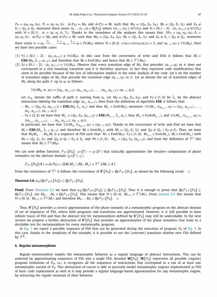
In Fig. 7 we report a possible sequence of FSA that can be generated during the execution of program P0 of Fig. 3. In this case, thanks to the simplicity of the example, it is possible to use the (concrete) transition relation over FSA defined by T F .
6. Regular metamorphism
Regular metamorphism models the metamorphic behavior as a regular language of abstract instructions. This can be achieved by approximating sequences of FSA into a single FSA, denoted W� P0 �. W� P0 � represents all possible (regular) program evolutions of P0, i.e., it recognizes all the sequences of instructions that correspond to a run of at least one metamorphic variant of P0. This abstraction of course is able to precisely model metamorphic engines implemented as FSA of basic code replacement as well as it may provide a regular language-based approximation for any metamorphic engine, by extracting the regular invariant of their behavior.

88 M. Dalla Preda et al. / Theoretical Computer Science 577 (2015) 74–97
Fig. 7. Some metamorphic variants of program P0 of Fig. 3, where the metamorphic engine, namely the instructions stored at locations from 8 to 14, is briefly represented by the box marked ME. In the graphic representation of automata we omit to show the nodes that are not reachable.
We define an ordering relation on FSA according to the language they recognize: Given two FSA M1 and M2 we say that M1 F M2 if L(M1) ⊆ L(M2). Observe that F is reflexive and transitive but not antisymmetric and it is therefore a pre-order. Moreover, according to this ordering, a unique least upper bound of two automata M1 and M2 does not always exist, since there is an infinite number of automata that recognize the language L(M1) ∪ L(M2). Given two automata M1 = (Q 1, δ1, S1, F1, A) and M2 = (Q 2, δ2, S2, F2, A) on the same alphabet A, we approximate their least upper bound with:
M1 � M2 = (Q 1 ∪ Q 2, δ, S1 ∪ S2, F1 ∪ F2, A)
where the transition relation δ : (Q 1 ∪ Q 2) × A → ℘(Q 1 ∪ Q 2) is defined as δ(q, s) = δ1(q, s) ∪ δ2(q, s). FSA are �-closed for finite sets, and the following result shows that � approximates any upper bound with respect to the ordering F .
Lemma 6.1. Given two FSA M1 and M2 we have: L(M1) ∪ L(M2) ⊆ L(M1 � M2).
Proof. Let us show by induction on the length of ω ∈ A∗ that for every q1 ∈ S1 it holds that q ∈ δ1(q1, ω) ⇒ q ∈ δ(q1, ω). Base: When |ω| = 1 we have that ω = s ∈ A and therefore δ1(q1, s) ⊆ δ1(q1, s) ∪ δ2(q1, s) = δ(q1, s). Assume that it holds for strings of length n and let us prove that it holds for strings of length n + 1. Let ω = s0 . . . sn−1sn . By definition we have that:
δ∗1(q1, s0 . . . sn−1sn) =
⋃p∈δ∗
1(q1,s0...sn−1)
δ(p, sn)
δ∗(q1, s0 . . . sn−1sn) =⋃
p∈δ∗(q1,s0...sn−1)
δ(p, sn)
By induction hypothesis δ∗1(q1, s0 . . . sn−1) ⊆ δ∗(q1, s0 . . . sn−1), and since δ(p, sn) = δ1(p, sn) ∪ δ2(p, sn), we have
δ∗1(q1, s0 . . . sn−1sn) ⊆ δ∗(q1, s0 . . . sn−1sn). Moreover the final states of M1 � M2 are F1 ∪ F2 and therefore: δ∗
1(q1, ω) ∩F1 �= ∅ ⇒ δ∗(q1, ω) ∩ (F1 ∪ F2) �= ∅. The proof that ∀q2 ∈ S2 : q ∈ δ2(q2, ω) ⇒ q ∈ δ(q2, ω) is analogous. �
M. Dalla Preda et al. / Theoretical Computer Science 577 (2015) 74–97 89
We can now define the function F�T � � P0 � : F → F as follows:
F�T � � P0 �(M) = α(P0)� M � (�{M ′ | M ′ ∈ T �(M)})
Observe that the set of possible successors of a given automaton M , i.e., T �(M), is finite since we have a (finite family of) successor for every transition edge of M and M has a finite set of edges. Since FSA are �-closed for finite sets, the function F�T � � P0 � is well defined and returns an FSA. Let ℘F (F∗) denote the domain of finite sets of strings of FSA, let K ∈ ℘F (F∗)
and let us define the function αS : ℘F (F∗) → F as:
αS(M0 . . . Mk) = �{Mi | 0 ≤ i ≤ k}αS(K ) = �{αS(M0 . . . Mk) | M0 . . . Mk ∈ K }
Function αS is additive and thus it defines a Galois connection (℘F (F∗), αS , γS , F). The following result shows that, when considering finite sets of sequences of FSA, the abstract function F�
T � � P0 � correctly approximates function FT � � P0 � on F.
Theorem 6.2. For any K ∈ ℘F (F∗): αS (FT � � P0 �(K )) F F�T � � P0 �(αS(K )).
Proof. We prove L(αS(FT � � P0 �(K ))) ⊆ L(F�T � � P0 �(αS (K ))). Let I0 . . . In ∈ L(αS (FT � � P0 �(K ))). This means ∃M0 . . . Mh ∈
FT � � P0 �(K ) with α(P0) = M0 s.t. I0 . . . In ∈ L(αS (M0 . . . Mh)). Let ∀i ∈ [0, h] : Mi = (Q i, Ei, Si). Therefore, by definition of FT � � P0 � and of �, we have that ∃M0 . . . Mh−1 ∈ K with α(P0) = M0 and Mh ∈ T �(Mh−1) such that I0 . . . In ∈ L((Q 0 ∪ . . .∪Q h), (E0 ∪ . . .∪ Eh), (S0 ∪ . . .∪ Sh)). Since M0 . . . Mh−1 ∈ K we have that αS (K ) = (Q K , E K , S K ) where Q 0 ∪ . . .∪ Q h−1 ⊆ Q K , E0 ∪ . . . ∪ Eh−1 ⊆ E K and S0 ∪ . . . ∪ Sh−1 ⊆ S K . This implies that Mh ∈ T �(αS(K )). By definition F�
T � � P0 �(αS(K )) = α(P0) �αS(K ) � (�{M ′ | M ′ ∈ T �(αS (K ))}), and therefore we have F�
T � � P0 �(αS (K )) = (Q ′, E ′, S ′) where Q 0 ∪ . . .∪ Q h−1 ∪ Q h ⊆ Q ′ , E0 ∪ . . . ∪ Eh−1 ∪ Eh ⊆ E ′ and S0 ∪ . . . ∪ Sh−1 ∪ Sh ⊆ S ′ and therefore I0 . . . In ∈ L(F�
T � � P0 �(αS(K ))). �Observe that, thanks to the fact that T �(M) returns a finite number of possible successors of M , then at each step of
the fix-point computation of FT � the function FT � is applied to a finite set of traces of FSA. This means Theorem 6.2 can be applied to each step of the fix-point computation of FT � .
The domain 〈F, F〉 has infinite ascending chains, which means that, in general, the fix-point computation of F�T � � P0 �
on F may not converge. A typical solution for this situation is the use of a widening operator which forces convergence towards an upper approximation of all intermediate computations along the fix-point iteration, i.e., an element in F which upper approximates the iterations of the fix-point semantic operator. The widening operator has for example been used to approximate fix-point computations in possibly non-complete lattices, e.g., in the case of convex polyhedra [15]. We refer to the widening operation over FSA described by D’Silva [22]. Here the author considers an increasing sequence M0 M1 . . . Mkof FSA in a fix-point computation of a function H on automata, where L(Mi+1) = L(Mi) ∪ L(H(Mi)). Given two FSA over a finite alphabet A in the considered sequence Mi = (Q i, Ei, Si) and M j = (Q j, E j, S j) with i < j, the widening between Mi and M j is formalized in terms of an equivalence relation R ⊆ Q i × Q j between the set of states of the two automata. The equivalence relation R , also called widening seed, is used to define another equivalence relation ≡R⊆ Q j × Q j over the states of M j , such that ≡R= R ◦ R−1. The widening between Mi and M j is then given by the quotient of M j with respect to the partition induced by ≡R :
Mi�M j = M j/≡R
By changing the widening seed, i.e., the equivalence relation R , we obtain different widening operators. It has been proved that convergence is guaranteed when the widening seed is the relation Rn ⊆ Q i × Q j such that (qi, q j) ∈ Rn if qi and q jrecognize the same language of strings of length at most n [22]. When considering the widening seed Rn we have that two states q and q′ of M j are in equivalence relation ≡Rn if they recognize the same language of strings of length at most n that is recognized by a state r of Mi , i.e., if ∃r ∈ Q i : (r, q) ∈ Rn and (r, q′) ∈ Rn . Thus, the parameter n tunes the length of the strings that we consider for establishing the equivalence of states and therefore for merging them in the widening, namely the more abstract will be the result of the widening. Observe that the smaller is n the more information will be lost by the widening. We denote with �n the widening operator that uses Rn as widening seed. �n is well defined since I is finite.
The widening operator �n allows us to approximate the least fix-point of F�T � � P0 � on 〈Fk, F〉 with the limit W� P0 �
of the following widening sequence:
W0 = α(P0) W i+1 = W i �n F�T � � P0 �(W i)
In the following we refer to W� P0 � as the widened fix-point of F�T � � P0 � and to the sequence W0 W1, . . . as the widening
sequence of F�T � � P0 �, namely the sequence of automata generated in the above widening fix-point computation. From the
correctness of the widening operator �n and by Theorem 6.2, it follows that the widening sequence W0 W1 . . . converges to an upper-approximation of the least fix-point of FT � � P0 �, namely any automata modeling a possible static variant of P0 is correctly approximated by W� P0 �. This means that for every Mi we have that:
90 M. Dalla Preda et al. / Theoretical Computer Science 577 (2015) 74–97
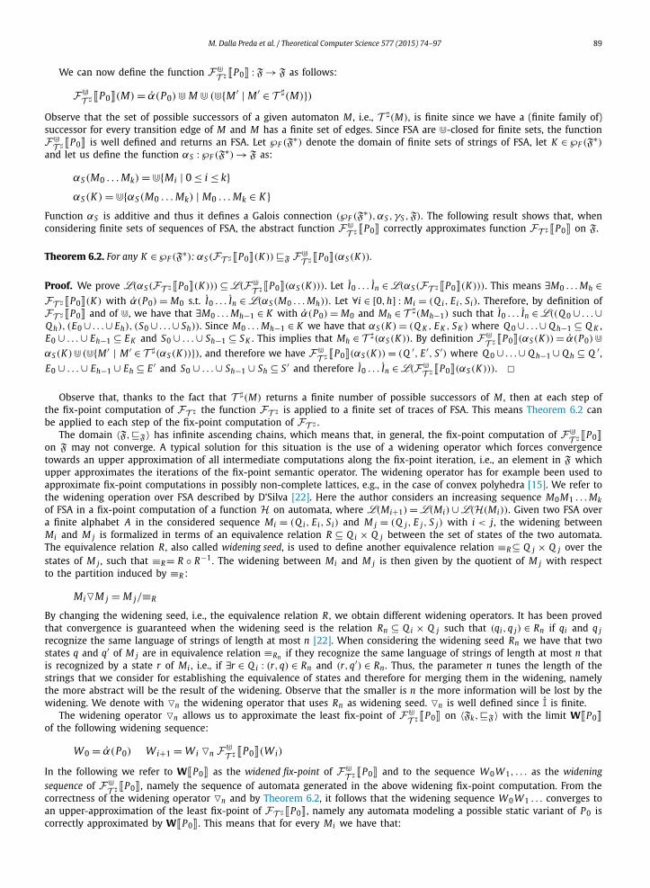
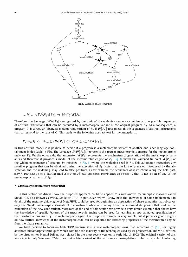
Fig. 8. Widened phase semantics.
. . . Mi . . . ∈ lfp⊆FT � � P0 � ⇒ Mi F W� P0 �
Therefore, the language L(W� P0 �) recognized by the limit of the widening sequence contains all the possible sequences of abstract instructions that can be executed by a metamorphic variant of the original program P0. As a consequence, a program Q is a regular (abstract) metamorphic variant of P0 if W� P0 � recognizes all the sequences of abstract instructions that correspond to the runs of Q . This leads to the following abstract test for metamorphism:
P0 �F Q ⇔ α(Q ) F W� P0 � ⇔ L(α(Q )) ⊆ L(W� P0 �)
In this abstract model it is possible to decide if a program is a metamorphic variant of another one since language con-tainment is decidable in FSA. The language L(W� P0 �) represents the regular metamorphic signature for the metamorphic malware P0. On the other side, the automaton W� P0 � represents the mechanism of generation of the metamorphic vari-ants and therefore it provides a model of the metamorphic engine of P0. Fig. 8 shows the widened fix-point W� P0 � of the widening sequence of program P0 reported in Fig. 3, where the widening seed is R2. This automaton recognizes any possible program that can be obtained during the execution of P0. Note that, the loss of precision introduced by the ab-straction and the widening, may lead to false positives, as for example the sequences of instructions along the bold path mov f , 100; input ⇒ a; MEM[a] mod 2 = 0; movb, MEM[a]; goto; movb, MEM[a]; goto; . . . that is not a run of any of the metamorphic variants of P0.
7. Case study: the malware MetaPHOR
In this section we discuss how the proposed approach could be applied to a well-known metamorphic malware called MetaPHOR, also known as Win32/Smile or ETAP. In particular, we will show how the knowledge of some implementation details of the metamorphic engine of MetaPHOR could be used for designing an abstraction of phase semantics that observes only the “final” metamorphic variants of the malware while abstracting from the intermediate phases that lead to the generation of the new code variant. Moreover, at the end of this section we provide a very simple example that shows how the knowledge of specific features of the metamorphic engine can be used for learning an approximated specification of the transformations used by the metamorphic engine. The proposed example is very simple but it provides good insights on how further knowledge of the metamorphic code can be exploited for extracting properties of the metamorphic engine from the phase semantics.
We have decided to focus on MetaPHOR because it is a real metamorphic virus that, according to [5], uses highly advanced metamorphic techniques which combine the majority of the techniques used by its predecessor. The virus, written by the virus writer Mental Driller, was released in the most recent version in early March 2002. The original version of this virus infects only Windows 32-bit files, but a later variant of the virus was a cross-platform infector capable of infecting

M. Dalla Preda et al. / Theoretical Computer Science 577 (2015) 74–97 91
also Linux ELF files. The Mental Driller named it MetaPHOR from the words “Metamorphic Permutating High-Obfuscating Reassembler”, which accurately describe this virus. A detailed description of the virus can be found at [5,21].2
Let us describe the main stages of the life-cycle behavior of MetaPHOR. Polymorphic Decryption: MetaPHOR starts by running a sophisticated polymorphic decryptor that hides from decryption heuristic scanners. Sometimes this step is not necessary because the virus could be unencrypted, as MetaPHOR is programmed to produce an unencrypted copy every few infections. Payload: MetaPHOR performs the intended payload that consists in displaying a specific message according to the current date. Re-building by metamorphism: MetaPHOR builds a new virus body in memory at each generation. The metamorphic process is very complex and accounts for around 70% of the viral code. Polymorphism: MetaPHOR uses ad-vanced polymorphic techniques such as the branching technique, pseudo-random index decryption technique (PRIDE) and entry point obscuring technique (EPO), see [5,19,20] for details. Infection: MetaPHOR searches for Win32 PE executable files in the current directory and in the directories located in the three levels above the current directory. The virus checks sev-eral things before infecting a file: For example it avoids to infect “goat” or “bait” files – files that are created by anti-virus programs.
7.1. The re-building engine of MetaPHOR
An innovative feature of the metamorphic re-building engine of MetaPHOR is the use of an intermediate representationwhich allows to abstract from the complexity of the underlying processor’s instruction-set and to simplify the metamor-phic transformations. In particular, the instruction-set of the intermediate representation includes: base instructions with 2 operands, such as: add, sub, or, and, mov, ... , base instructions with 1 operand, such as: push, pop, call, ... , other instructions, such as: ret, lea, ... and macro-instructions that represent for example the instruction sequences which are used when calling a Windows API (such as apicall-begin, apicall-end), or a system call, or a system call followed by the results saving and so on. Once MetaPHOR has decrypted its own code, it gives control to it and, after the potential payload actions, it re-builds its own code by applying metamorphic transformations. The re-building process is organized as follows:
• Disassembly-Depermutation: The x86 code is first disassembled into the intermediate representation presented above. The disassembly algorithm builds the intermediate code in a linear way and this ensures both the depermutation of the resulting code and the removal of the inaccessible code (dead code).
• Compression: This step is necessary in order to avoid continuous growth of the viral code that would lead to a virus of many mega-bytes in very few generations. The basic idea of this process is to compress in one instruction what the expansion process codes in many. This is achieved by applying transformations that are the inverse of the ones used by the expansion process. Examples of compressing transformations are:1. Rules that transform one instruction into an equivalent one, as for example:
– sub e, imm−→ add e, −imm– or e, 0 −→ nop
2. Rules that transform a sequence of two instructions into one instruction, as for example:– push imm; pop e −→ mov e, imm– mov e, imm; push e −→ push imm
– op e, imm; op e, imm2−→ op e, (imm op imm2)3. Rules that transform a sequence of three instructions into one instruction, as for example:
– mov e1, e2; op e1, e3; mov e2, e1 −→ op e2, e3
Compression corresponds to rewriting code in such a way that we substitute the first instructions by their equivalent one according to the rule and we overwrite the remaining instructions with nop. The compression algorithm com-presses the code as much as possible by iterating the code rewriting process. A complete list of the compression rules used by MetaPHOR can be found in [21]. In the following we report an example of what a compressor does in few iterations:
mov [var1], esi mov eax, esipush [var1] noppop eax �⇒ noppush ebx add eax, ebxpop [var2] nopadd eax, [var2] nop
2 The assembly code of the virus can be found at: http://vx.netlux.org/29a/29a-6/29a-6.602.
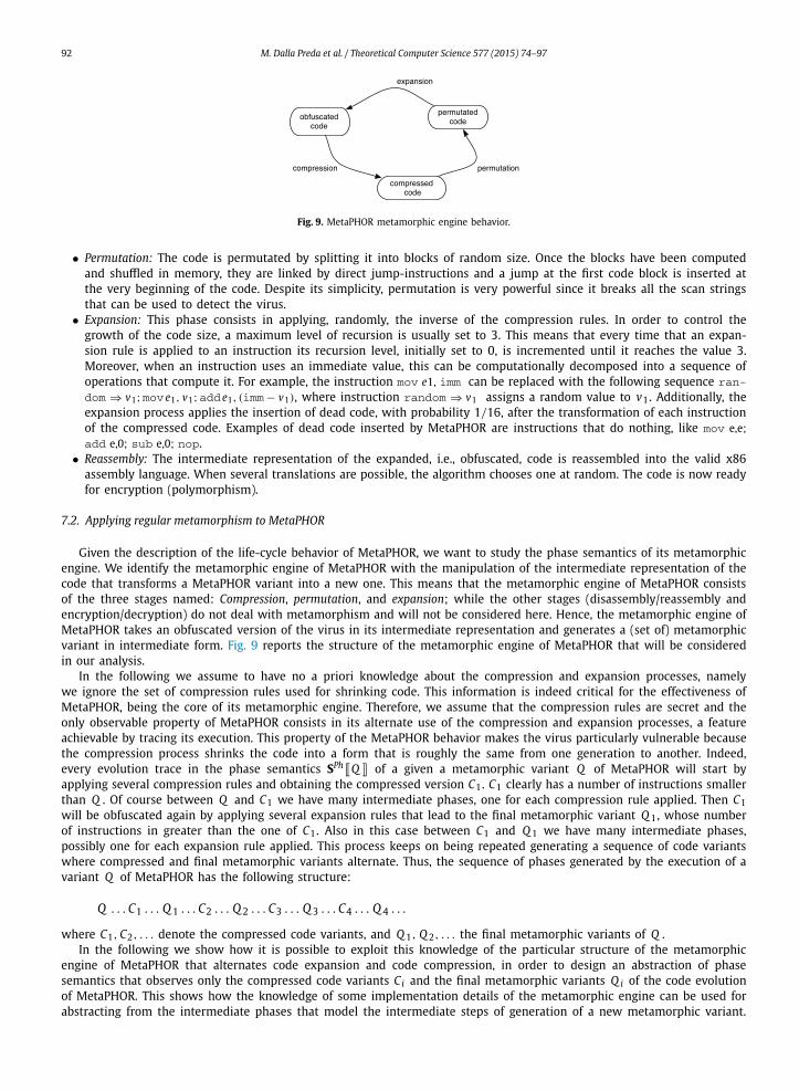
92 M. Dalla Preda et al. / Theoretical Computer Science 577 (2015) 74–97
Fig. 9. MetaPHOR metamorphic engine behavior.
• Permutation: The code is permutated by splitting it into blocks of random size. Once the blocks have been computed and shuffled in memory, they are linked by direct jump-instructions and a jump at the first code block is inserted at the very beginning of the code. Despite its simplicity, permutation is very powerful since it breaks all the scan strings that can be used to detect the virus.
• Expansion: This phase consists in applying, randomly, the inverse of the compression rules. In order to control the growth of the code size, a maximum level of recursion is usually set to 3. This means that every time that an expan-sion rule is applied to an instruction its recursion level, initially set to 0, is incremented until it reaches the value 3. Moreover, when an instruction uses an immediate value, this can be computationally decomposed into a sequence of operations that compute it. For example, the instruction mov e1, imm can be replaced with the following sequence ran-dom ⇒ v1; mov e1, v1; add e1, (imm− v1), where instruction random ⇒ v1 assigns a random value to v1. Additionally, the expansion process applies the insertion of dead code, with probability 1/16, after the transformation of each instruction of the compressed code. Examples of dead code inserted by MetaPHOR are instructions that do nothing, like mov e,e;add e,0; sub e,0; nop.
• Reassembly: The intermediate representation of the expanded, i.e., obfuscated, code is reassembled into the valid x86 assembly language. When several translations are possible, the algorithm chooses one at random. The code is now ready for encryption (polymorphism).
7.2. Applying regular metamorphism to MetaPHOR
Given the description of the life-cycle behavior of MetaPHOR, we want to study the phase semantics of its metamorphic engine. We identify the metamorphic engine of MetaPHOR with the manipulation of the intermediate representation of the code that transforms a MetaPHOR variant into a new one. This means that the metamorphic engine of MetaPHOR consists of the three stages named: Compression, permutation, and expansion; while the other stages (disassembly/reassembly and encryption/decryption) do not deal with metamorphism and will not be considered here. Hence, the metamorphic engine of MetaPHOR takes an obfuscated version of the virus in its intermediate representation and generates a (set of) metamorphic variant in intermediate form. Fig. 9 reports the structure of the metamorphic engine of MetaPHOR that will be considered in our analysis.
In the following we assume to have no a priori knowledge about the compression and expansion processes, namely we ignore the set of compression rules used for shrinking code. This information is indeed critical for the effectiveness of MetaPHOR, being the core of its metamorphic engine. Therefore, we assume that the compression rules are secret and the only observable property of MetaPHOR consists in its alternate use of the compression and expansion processes, a feature achievable by tracing its execution. This property of the MetaPHOR behavior makes the virus particularly vulnerable because the compression process shrinks the code into a form that is roughly the same from one generation to another. Indeed, every evolution trace in the phase semantics SPh � Q � of a given a metamorphic variant Q of MetaPHOR will start by applying several compression rules and obtaining the compressed version C1. C1 clearly has a number of instructions smaller than Q . Of course between Q and C1 we have many intermediate phases, one for each compression rule applied. Then C1will be obfuscated again by applying several expansion rules that lead to the final metamorphic variant Q 1, whose number of instructions in greater than the one of C1. Also in this case between C1 and Q 1 we have many intermediate phases, possibly one for each expansion rule applied. This process keeps on being repeated generating a sequence of code variants where compressed and final metamorphic variants alternate. Thus, the sequence of phases generated by the execution of a variant Q of MetaPHOR has the following structure:
Q . . . C1 . . . Q 1 . . . C2 . . . Q 2 . . . C3 . . . Q 3 . . . C4 . . . Q 4 . . .
where C1, C2, . . . denote the compressed code variants, and Q 1, Q 2, . . . the final metamorphic variants of Q .In the following we show how it is possible to exploit this knowledge of the particular structure of the metamorphic
engine of MetaPHOR that alternates code expansion and code compression, in order to design an abstraction of phase semantics that observes only the compressed code variants Ci and the final metamorphic variants Q i of the code evolution of MetaPHOR. This shows how the knowledge of some implementation details of the metamorphic engine can be used for abstracting from the intermediate phases that model the intermediate steps of generation of a new metamorphic variant.
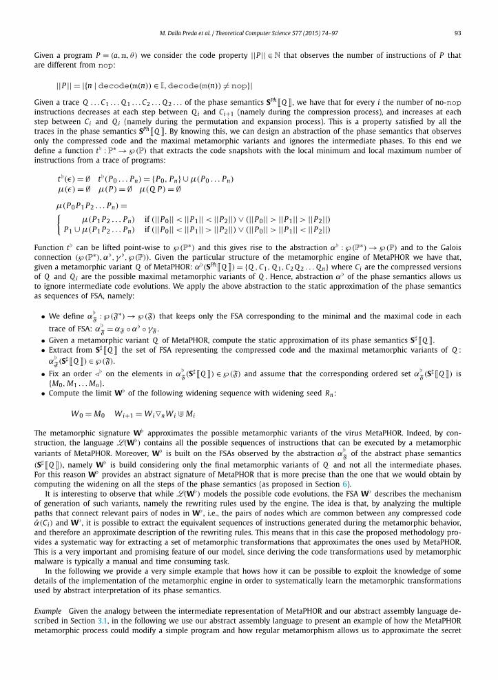
M. Dalla Preda et al. / Theoretical Computer Science 577 (2015) 74–97 93
Given a program P = (a, m, θ) we consider the code property ||P || ∈ N that observes the number of instructions of P that are different from nop:
||P || = |{n | decode(m(n)) ∈ I,decode(m(n)) �= nop}|Given a trace Q . . . C1 . . . Q 1 . . . C2 . . . Q 2 . . . of the phase semantics SPh � Q �, we have that for every i the number of no-nopinstructions decreases at each step between Q i and Ci+1 (namely during the compression process), and increases at each step between Ci and Q i (namely during the permutation and expansion process). This is a property satisfied by all the traces in the phase semantics SPh � Q �. By knowing this, we can design an abstraction of the phase semantics that observes only the compressed code and the maximal metamorphic variants and ignores the intermediate phases. To this end we define a function t� : P∗ → ℘(P) that extracts the code snapshots with the local minimum and local maximum number of instructions from a trace of programs:
t�(ε) = ∅ t�(P0 . . . Pn) = {P0, Pn} ∪ μ(P0 . . . Pn)
μ(ε) = ∅ μ(P ) = ∅ μ(Q P ) = ∅μ(P0 P1 P2 . . . Pn) ={
μ(P1 P2 . . . Pn) if (||P0|| < ||P1|| < ||P2||) ∨ (||P0|| > ||P1|| > ||P2||)P1 ∪ μ(P1 P2 . . . Pn) if (||P0|| < ||P1|| > ||P2||) ∨ (||P0|| > ||P1|| < ||P2||)
Function t� can be lifted point-wise to ℘(P∗) and this gives rise to the abstraction α� : ℘(P∗) → ℘(P) and to the Galois connection (℘ (P∗), α�, γ �, ℘(P)). Given the particular structure of the metamorphic engine of MetaPHOR we have that, given a metamorphic variant Q of MetaPHOR: α�(SPh � Q �) = {Q , C1, Q 1, C2 Q 2 . . . Q n} where Ci are the compressed versions of Q and Q i are the possible maximal metamorphic variants of Q . Hence, abstraction α� of the phase semantics allows us to ignore intermediate code evolutions. We apply the above abstraction to the static approximation of the phase semantics as sequences of FSA, namely:
• We define α�
F: ℘(F∗) → ℘(F) that keeps only the FSA corresponding to the minimal and the maximal code in each
trace of FSA: α�
F= αF ◦ α� ◦ γF .
• Given a metamorphic variant Q of MetaPHOR, compute the static approximation of its phase semantics S� � Q �.• Extract from S�� Q � the set of FSA representing the compressed code and the maximal metamorphic variants of Q :
α�
F(S�� Q �) ∈ ℘(F).
• Fix an order �� on the elements in α�
F(S�� Q �) ∈ ℘(F) and assume that the corresponding ordered set α�
F(S�� Q �) is
{M0, M1 . . . Mn}.• Compute the limit W� of the following widening sequence with widening seed Rn:
W0 = M0 W i+1 = W i�n W i � Mi
The metamorphic signature W� approximates the possible metamorphic variants of the virus MetaPHOR. Indeed, by con-struction, the language L(W�) contains all the possible sequences of instructions that can be executed by a metamorphic variants of MetaPHOR. Moreover, W� is built on the FSAs observed by the abstraction α�
Fof the abstract phase semantics
(S�� Q �), namely W� is build considering only the final metamorphic variants of Q and not all the intermediate phases. For this reason W� provides an abstract signature of MetaPHOR that is more precise than the one that we would obtain by computing the widening on all the steps of the phase semantics (as proposed in Section 6).
It is interesting to observe that while L(W�) models the possible code evolutions, the FSA W� describes the mechanism of generation of such variants, namely the rewriting rules used by the engine. The idea is that, by analyzing the multiple paths that connect relevant pairs of nodes in W� , i.e., the pairs of nodes which are common between any compressed code α(Ci) and W� , it is possible to extract the equivalent sequences of instructions generated during the metamorphic behavior, and therefore an approximate description of the rewriting rules. This means that in this case the proposed methodology pro-vides a systematic way for extracting a set of metamorphic transformations that approximates the ones used by MetaPHOR. This is a very important and promising feature of our model, since deriving the code transformations used by metamorphic malware is typically a manual and time consuming task.
In the following we provide a very simple example that hows how it can be possible to exploit the knowledge of some details of the implementation of the metamorphic engine in order to systematically learn the metamorphic transformations used by abstract interpretation of its phase semantics.
Example Given the analogy between the intermediate representation of MetaPHOR and our abstract assembly language de-scribed in Section 3.1, in the following we use our abstract assembly language to present an example of how the MetaPHOR metamorphic process could modify a simple program and how regular metamorphism allows us to approximate the secret
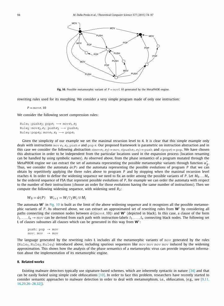
94 M. Dalla Preda et al. / Theoretical Computer Science 577 (2015) 74–97
Fig. 10. Possible metamorphic variant of P = mov l,10 generated by the MetaPHOR engine.
rewriting rules used for its morphing. We consider a very simple program made of only one instruction:
P = mov e,10
We consider the following secret compression rules:
Rule1 : push e2; pop e1 −→ mov e1, e2
Rule2 : mov e2, e1; push e2 −→ push e1
Rule3 : pop e2; mov e1, e2 −→ pop e1
Given the simplicity of our example we set the maximal recursion level to 4. It is clear that this simple example only deals with instructions mov e1, e2, push e and pop e. Our proposed framework is parametric on instruction abstraction and in this case we consider the following abstraction ι(mov e1, e2) = mov, ι(push e1, e2) = push and ι(pop e) = pop. We have chosen this abstraction in order to be independent from the particular locations used in the expansion process (location renaming can be handled by using symbolic names). As observed above, from the phase semantics of a program mutated through the MetaPHOR engine we can extract the set of automata representing the possible metamorphic variants through function α
�
F.
Thus, we consider the automata α(P ) and the automata representing the possible evolutions of program P that we can obtain by repetitively applying the three rules above to program P and by stopping when the maximal recursion level reaches 4. In order to define the widening sequence we need to fix an order among the possible variants of P . Let M0 . . . Mn
be the ordered sequence of FSA that represent possible evolutions of P , for example we can order the automata with respect to the number of their instructions (choose an order for those evolutions having the same number of instructions). Then we compute the following widening sequence, with widening seed R2:
W0 = α(P ) W i+1 = W i�2W i � Mi
The automata W� in Fig. 10 is built as the limit of the above widening sequence and it recognizes all the possible metamor-phic variants of P . As observed above, we can extract an approximated set of rewriting rules from W� by considering all paths connecting the common nodes between α({mov e,10}) and W� (depicted in black). In this case, a clause of the form I1, . . . , In → mov can be derived from each path with instruction-labels I1, . . . , In connecting black nodes. The following set Ł of clauses subsumes all clauses which can be generated in this way from W�:
push ; pop → movmov ; mov → mov
The language generated by the rewriting rules Ł includes all the metamorphic variants of mov generated by the rules {Rule1, Rule2, Rule3} introduced above, including spurious sequences like mov mov mov mov induced by the widening approximation. This shows how the analysis of the phase semantics of a metamorphic virus can provide important informa-tion about the implementation of its metamorphic engine.
8. Related works
Existing malware detectors typically use signature-based schemes, which are inherently syntactic in nature [34] and that can be easily fooled using simple code obfuscations [10]. In order to face this problem, researchers have recently started to consider semantic approaches to malware detection in order to deal with metamorphism, i.e., obfuscation, (e.g., see [9,11,16,29,26–28,32]).
M. Dalla Preda et al. / Theoretical Computer Science 577 (2015) 74–97 95
In [16] the authors use trace semantics to characterize the behaviors of the malware and of the potentially infected program, and use abstract interpretation to “hide” irrelevant aspects of these behaviors. In this setting, a program is infected by a malware if their behaviors are indistinguishable up to a certain abstraction, which corresponds to some obfuscations. A significant limitation of this work, however, is that it does not give any systematic method to derive abstractions from obfuscations. The knowledge of the obfuscation is essential in order to derive these abstractions.
In [27] the authors model the malware as a formula in the new logic CTPL, which is an extension of CTL able to handle register renaming. They develop a model checking algorithm for CTPL and use it to verify infection. A program P is infected by malware M , if P satisfies the CTPL formula that models M . By knowing the obfuscations used by malware M it is possible to design CTPL specifications that recognize several metamorphic variants of M . Once again the knowledge of the obfuscations is essential in order to check infection.
In [11] the idea is to model the malware as a template that expresses its malicious intent, while no distinction is made among their different metamorphic variants. Also in this case the definition of the template is driven by the knowledge of the obfuscations commonly used by malware: It uses symbolic variable/constants to handle variable and register renaming, and it is related to the malware control flow graph in order to deal with code reordering. The authors provide an algorithm that verifies whether a program presents the considered template malicious behavior, and in the case of positive answer they classify the program as infected.
In [28] the authors propose a methodology for making context-sensitive analysis of assembly programs even when the call and ret instructions are obfuscated. In particular, they define a general framework where they formalize the notion of context-trace semantics. They show how, by successive abstractions of the context-trace semantics, it is possible to derive by abstract interpretation the context-sensitive version of any context insensitive analysis that was obtained by approximating the context insensitive trace semantics.
Some researchers have tried to detect metamorphic malware by modeling the metamorphic engine as formal grammars and automata [23,31,35]. These works are promising but the design of the grammar and automata is based on the knowl-edge of the metamorphic transformations used, and none of them provides a methodology for extracting a grammar or an automata from a given metamorphic malware.
In [6] the authors use FSA to approximate programs in a setting that is different from ours. In particular, Beaucamps et al. approximate the set of possible execution traces of a program with a regular language P on a given alphabet that expresses some instruction properties (like being a system call). In order to be independent from implementation details (and therefore cope with metamorphism) the regular language P is abstracted with respect to predefined behavioral patterns. A behavioral pattern is formalized as an automata whose regular language Bλ ∈ ℘( ∗) describes the possible sequences in ∗ that satisfy a high level property λ. The abstraction of P with respect to Bλ is obtained by replacing in each trace of P all the occurrences of the patterns of Bλ with λ. This abstraction can be carried out with respect to all the behavioral patterns Bλ1 . . .Bλn representing high level properties of interest. This leads to a description of the original program as a regular language of abstract symbols � = {λ1 . . . λn} that can be compared to the abstract description of known malware in order to detect infection. This detection strategy is able to recognize all the metamorphic variants that are considered by the behavioral patterns. Thus, in order to design efficient behavioral patterns we need to know in advance the metamorphic transformations used by malware. In the experiments in [6] the authors construct the behavioral patterns from the observation of some known malicious execution traces. We believe that it is possible to use our method based on abstracting the phase semantics to systematically derive the FSA for Bλ .
In [1,2] the authors model malware as tree automata and then use tree automata inference for capturing the essence of being malicious. Their idea is to focus on the system call behaviour of the malware and to use dynamic analysis in order to extract the data flow dependences between system calls. These dependences are then represented as a graph that provides an abstract model of the malicious behaviour. Next, given a set of these system call dependences graphs, they use tree automata inference to derive (learn) an automata that is able to recognize them. This automata should ideally capture the essence of the malicious behavior and should be able to detect also unknown variants of the considered malware. In our framework we would say that the learned automata acts like a metamorphic signature for the set of malware variants from which it has been generated. However, it cannot be ensured that the so obtained metamorphic signature is able to capture all the possible variants of a given malware. Indeed the efficiency of the automata in capturing unknown malware depends on the malware set used for training the inference algorithm.
All these approaches provide a model of the metamorphic behavior that is based on the knowledge of the metamorphic transformations, i.e., obfuscations, that malware typically use. By knowing how code mutates, it is possible to specify suitable (semantics-based) equivalence relations which trace code evolution and detect malware. This knowledge is typically the result of a time and cost consuming tracking analysis based on emulation and heuristics, which requires intensive human interaction in order to achieve an abstract specification of code features that are common to the malware variants obtained through various obfuscations and mutations. These abstract specifications of the malicious behavior are designed based on the obfuscations used by malware and can therefore be potentially bypassed by the design of a variety of new evasion techniques, yet keeping the basic attack model unchanged.
A work closed to our is the one proposed by Guizani et al. [25]. Here the authors propose a theoretical framework for modeling self-modifying programs. They introduce the notion of code waves which are very similar to our phases. The main difference is that their approach for modeling code evolution is dynamic while our one is static. So they can might be more
96 M. Dalla Preda et al. / Theoretical Computer Science 577 (2015) 74–97
precise on the analysis of the considered execution traces but they have to face the problem of behavioral coverage typical of dynamic analysis.
To the best of our knowledge, we are not aware of any work for statically modeling metamorphism without any a priori knowledge of the transformations used by the metamorphic engine.
Another important work that formally addresses the analysis of self-modifying code is the one of Cai et al. [8]. In this work the authors propose a general framework based on Hoare logic for the modular verification of self-modifying programs. In particular, in order to reason on self-modifying code Cai et al. treat code as data and apply separation logic to support local reasoning in order to verify code modules and then combine them through the frame rule. A related recent work in the verification of self-modifying x86 code based on Hoare logic is the one of Myreen [30]. Myreen proposes a formal semantics for x86 that models possible out-of-date instruction cache and defines a Hoare logic on this semantics that allows to reason about self-modifying code. However, their goals and results are very different from ours: Cai et al. and Myreen propose a general framework based on Hoare logic to verify self-modifying code, while we use program semantics and abstract interpretation to extract metamorphic signature from malicious self-modifying code.
9. Discussion
While traditional static models of programs consider programs that have a constant structure during execution, meta-morphic attacks require new semantic models and analysis for coping with unknown obfuscation strategies, generated by an unknown metamorphic engine. In order to model the self-modifying nature of a metamorphic malware it is necessary to provide a model of program behavior that allows the program to change during execution. For this reason we have intro-duced the notion of phase semantics, that precisely describes the evolution of any metamorphic program during execution. Phase semantics allows us to model the self-modifying behavior of any metamorphic malware and it does not need any a priori knowledge of the metamorphic transformations. The key contribution relies upon the idea that abstract interpreta-tion of phase semantics provides useful information about the way code changes, i.e., about the metamorphic engine itself, without any a priori knowledge on its concrete implementation. Phase semantics provides a very precise and low level description of the metamorphic behavior, and due to the presence of possible infinite sequences of code evolution it may not be possible to decide whether a program appears in the phase semantics of another one, namely whether a program is a metamorphic variant of another one. Since we are interested in deciding this fact we recurred to abstract interpretation in order to loose some of the precision of phase semantics in favor of decidability. In particular, the abstract interpretation of the phase semantics of a metamorphic program P on the abstract domain of FSA, i.e., automaton W� P �, provides an abstract metamorphic signature that can be used to verify if a program is a metamorphic variant of P . The idea is that the language recognized by the resulting automaton represents the sequences of all possible instructions that can be en-countered during the execution of a variant of the original code. A priori knowledge of the transformations applied by the metamorphic engine can be used to further abstract the FSA-representation and to obtain an FSA that models in a more concise way all the possible metamorphic variants. For example, by abstracting from the intermediate phases that model the intermediate steps of code mutation that lead to the generation of a metamorphic code variant.
Interestingly, the language recognized by W� P � provides an upper-approximation of the possible metamorphic variants of the original malware, while the automaton itself models the mechanism of generation of such variants, i.e., an approx-imation of the metamorphic engine. This means that with our approach it should be possible to extract properties of the implementation of the metamorphic engine by abstract interpretation of the phase semantics. In Section 7 we have con-sidered the malware MetaPHOR and we have shown how to learn the metamorphic engine from phase semantics on toy example. Besides its simplicity, this example provides good insights on how to proceed for the extraction of properties of code evolution from phase semantics. The idea is that phase semantics captures all the details of code evolution and in order to extract properties of this evolution we need to know what to look at, namely what to observe and what to abstract from. Indeed, we need to design a proper abstraction of code that it is suitable for the property of interest. Any information regarding features of the metamorphic engine can be useful in the design of such an abstraction.
The phase semantics provides a semantics-based model for code metamorphism where abstract interpretation is used for reasoning about code layout. This opens an interesting new field that may represent a future challenge for abstract interpre-tation: The abstraction of code layout, where the code is the object of abstraction and the way it is generated is the object of abstract interpretation. The computation of the phase semantics on these abstract domains returns an approximation of the possible evolutions of the malicious code, where the code variants are approximated with objects of the abstract domain. As future work we are interested in using these approximated code variants in order to extract a formal specification of all possible code variants that could be generated and of the metamorphic engine. The idea is to consider known algorithms for learning from positive examples and to adapt them to the extraction of common features among variants of metamorphic malware. For example we could model the metamorphic engine as a rewriting system, an automata, a grammar or a logic program and then develop a learning strategy for the extraction of upper approximating term rewriting systems, automata and grammars incorporating the provided positive examples yet inducing an approximation of the metamorphic mutation engine. Particular emphasis will be devoted to extract context-free grammars modeling code mutations driven by context free rewriting rules. This involves the definition of widening operators, namely a transformation which steady unstable sub-strings characterizing exactly the invariant part of the unstable strings of a self-mutating malware. We then plan to validate these learning methodology on real malware.
M. Dalla Preda et al. / Theoretical Computer Science 577 (2015) 74–97 97
We believe that the possibility of understanding properties of the implementation of the metamorphic engine, by analyz-ing the structure of an approximate specification derived by abstract interpretation from the phase semantics of a malware (e.g., the FSA W� P �), will become an essential tool for a quick tracking of malicious code and for understanding new obfuscation strategies in the long standing battle between hiding and seeking in computer security.
Acknowledgements
The work of Mila Dalla Preda was partially supported by the MIUR FIRB 2013 project FACE (Formal Avenue for Chasing malwarE) RBFR13AJFT.
We would like to thank the anonymous referees for their useful comments that have helped us in improving the paper.
References
[1] D. Babic, D. Reynaud, D. Song, Malware analysis with tree automata inference, in: Proceedings of the Computer Aided Verification – 23rd International Conference, CAV 2011, in: Lecture Notes in Computer Science, vol. 6806, Springer, 2011, pp. 116–131.
[2] D. Babic, D. Reynaud, D. Song, Recognizing malicious software behaviors with tree automata inference, Form. Methods Syst. Des. 41 (1) (2012) 107–128.[3] G. Balakrishnan, R. Gruian, T.W. Reps, T. Teitelbaum, Codesurfer/x86 – a platform for analyzing x86 executables, in: Proceedings of the 14th Interna-
tional Conference on Compiler Construction, CC’05, 2005, pp. 250–254.[4] G. Balakrishnan, T.W. Reps, Analyzing memory accesses in x86 executables, in: Proceedings of the 13th International Conference on Compiler Construc-
tion, CC’04, 2004, pp. 5–23.[5] P. Beaucamps, Advanced metamorphic techniques in computer viruses, available at VX Heavens: http://vxheavens.com/lib/apb01.html, 2008.[6] P. Beaucamps, I. Gnaedig, J. Marion, Behavior abstraction in malware analysis, in: Proceedings of Runtime Verification – First International Conference,
RV10, in: Lecture Notes in Computer Science, vol. 6418, Springer, 2010, pp. 168–182.[7] D. Bruschi, L. Martignoni, M. Monga, Code normalization for self-mutating malware, IEEE Secur. Priv. 5 (2) (2007) 46–54.[8] H. Cai, Z. Shao, A. Vaynberg, Certified self-modifying code, in: Proceedings of the 2007 ACM SIGPLAN Conference on Programming Language Design
and Implementation, PLDI ’07, ACM, New York, NY, USA, 2007, pp. 66–77.[9] M. Christodorescu, S. Jha, Static analysis of executables to detect malicious patterns, in: Proceedings of the 12th USENIX Security Symposium, Secu-
rity ’03, 2003, pp. 169–186.[10] M. Christodorescu, S. Jha, Testing malware detectors, in: Proceedings of the ACM SIGSOFT International Symposium on Software Testing and Analysis,
ISSTA ’04, ACM, 2004, pp. 34–44.[11] M. Christodorescu, S. Jha, S.A. Seshia, D. Song, R.E. Bryant, Semantics-aware malware detection, in: Proceedings of the IEEE Symposium on Security and
Privacy, S&P’05, Oakland, CA, USA, 2005, pp. 32–46.[12] P. Cousot, R. Cousot, Abstract interpretation: a unified lattice model for static analysis of programs by construction or approximation of fixpoints, in:
Proceedings of the 4th ACM Symp. on Principles of Programming Languages, POPL ’77, ACM Press, New York, 1977, pp. 238–252.[13] P. Cousot, R. Cousot, Systematic design of program analysis frameworks, in: Proceedings of the 6th ACM Symp. on Principles of Programming Languages,
POPL ’79, ACM Press, New York, 1979, pp. 269–282.[14] P. Cousot, R. Cousot, Formal language, grammar and set-constraint-based program analysis by abstract interpretation, in: Proceedings of the Seventh
ACM Conference on Functional Programming Languages and Computer Architecture, La Jolla, California, 25–28 June 1995, ACM Press, New York, NY, 1995, pp. 170–181.
[15] P. Cousot, N. Halbwachs, Automatic discovery of linear restraints among variables of a program, in: Conference Record of the Fifth Annual ACM SIGPLAN-SIGACT Symposium on Principles of Programming Languages, Tucson, Arizona, ACM Press, New York, NY, 1978, pp. 84–97.
[16] M. Dalla Preda, M. Christodorescu, S. Jha, S. Debray, A semantics-based approach to malware detection, ACM Trans. Program. Lang. Syst. 30 (5) (2008) 1–54.
[17] M. Dalla Preda, R. Giacobazzi, S. Debray, K. Coogan, G. Townsend, Modelling metamorphism by abstract interpretation, in: Proceedings of the 17th International Static Analysis Symposium, SAS10, in: Lecture Notes in Computer Science, vol. 6337, Springer-Verlag, 2010, pp. 218–235.
[18] M. Dalla Preda, The grand challenge in metamorphic analysis, in: Proceedings of the 6th International Conference on Information Systems, Technology and Management, ICISTM’12, in: Communications in Computer and Information Science, vol. 285, Springer, 2012, pp. 439–444.
[19] Mental Driller, Advanced polymorphic engine construction. 29A E-zine, available at http://vx.netlux.org/lib/vmd03.html, 2000.[20] Mental Driller, Tuareg details and source code. 29A E-zine, available at http://vx.org.ua/29a/29A-5.html, 2000.[21] Mental Driller, How I made MetaPHOR and what I’ve learnt, available at VX Heavens: http://vxheavens.com/lib/vmd01.html, 2002.[22] V. D’Silva, Widening for automata, Diploma thesis, Institut Fur Informatick, Universitat Zurich, 2006.[23] E. Filiol, Metamorphism, formal grammars and undecidable code mutation, in: Proceedings of World Academy of Science, Engineering and Technology,
PWASET, vol. 20, 2007.[24] R. Giacobazzi, F. Ranzato, F. Scozzari, Making abstract interpretations complete, J. ACM 47 (2) (2000) 361–416.[25] W. Guizani, J. Marion, D. Reynaud-Plantey, Server-side dynamic code analysis, in: Proceedings of the 4th IEEE International Conference on Malicious an
Unwanted Software, MALWARE’09, 2009, pp. 55–62.[26] A. Holzer, J. Kinder, H. Veith, Using verification technology to specify and detect malware, in: Proceedings of the 11th International Conference on
Computer Aided System Theory, EUROCAST’07, in: LNCS, vol. 4739, 2007, pp. 497–504.[27] J. Kinder, S. Katzenbeisser, C. Schallhart, H. Veith, Detecting malicious code by model checking, in: Proceedings of the 2nd International Conference on
Intrusion and Malware Detection and Vulnerability Assessment, DIMVA’05, in: LNCS, vol. 3548, 2005, pp. 174–187.[28] A. Lakhotia, D. Boccardo, A. Singh, A. Manacero, Context-sensitive analysis of obfuscated x86 executables, in: Proceedings of the 2010 ACM SIGPLAN
Workshop on Partial Evaluation and Program Manipulation, PEPM 2010, ACM, 2010, pp. 131–140.[29] G. Lu, S. Debray, Automatic simplification of obfuscated javascript code: a semantics-based approach, in: Proceedings of the Sixth International Confer-
ence on Software Security and Reliability, SERE 2012, IEEE, 2012, pp. 31–40.[30] Magnus O. Myreen, Verified just-in-time compiler on x86, in: Proceedings of the 37th ACM SIGPLAN-SIGACT Symposium on Principles of Programming
Languages, POPL 2010, ACM, 2010, pp. 107–118.[31] Qozah, Polymorphism and grammars. 29A E-zine, 2009.[32] P. Singh, A. Lakhotia, Static verification of worm and virus behaviour in binary executables using model checking, in: Proceedings of the 4th IEEE
Information Assurance Workshop, 2003.[33] P. Ször, P. Ferrie, Hunting for metamorphic, in: Proceedings of the Virus Bulleting Conference, Virus Bulletin Ltd, 2001, pp. 123–144.[34] P. Ször, The Art of Computer Virus Research and Defense, Addison–Wesley Professional, Boston, MA, USA, 2005.[35] P. Zbitskiy, Code mutation techniques by means of formal grammars and automatons, J. Comput. Virol. (2009).