theoretical considerations of local environment...
TRANSCRIPT

Linkoping Studies in Science and TechnologyDissertation No. 1353
Theoretical Considerations of
Local Environment Effects in Alloys
Tobias Marten
Department of Physics, Chemistry and Biology (IFM)Linkoping University, SE-581 83 Linkoping, Sweden
Linkoping 2010

ISBN 978–91–7393–285–1ISSN 0345–7524
Printed by LiU-Tryck, Linkoping 2010

To my wife & ourlovely daughter

Abstract
This thesis is devoted to a theoretical study of local environment effects in alloys.A fundamental property of a disordered system is that all chemically equivalentatoms are different due to their different chemical environments, in contrast to anideal periodic solid where all the atoms that occupy equivalent positions in thecrystal have exactly the same physical properties. The local environment effectshave been largely ignored in earlier theories of disordered systems, that is thesystem has been treated as a whole and average properties have been derived.Moreover, inhomogeneous systems, such as surfaces and interfaces, induce localenvironment effects that are not necessarily present in the bulk.
The importance and presence of local environment effects are illustrated bycalculating observable physical properties in various systems. In particular, byemploying the complete screening picture the effects of local environments on thecore-level binding energy shifts as well as Auger shifts in random alloys are in-vestigated. This so-called disorder broadening effect has recently been observedexperimentally. It is shown that there are different contributions to the disorderbroadening that vary with the local chemical environment. Furthermore, the influ-ence of inhomogeneous lattice distortions on the disorder broadening of the core-level photoemission spectra are considered for systems with large size-mismatchbetween the alloy components.
The effects of local chemical environments on physical properties in magneticsystems are illuminated. A noticeable variation in the electronic structure, localmagnetic moments and exchange parameters at different sites is obtained. Thisreflects the sensitivity to different chemical environments and it is shown to be ofqualitative importance in the vicinity of magnetic instability.
The local environment effects due to the presence of surfaces and interfaces arealso considered. The effect is explicitly studied by considering the concentrationprofile of a thin Ag-Pd film deposited on a Ru substrate. Two computationalapproaches are utilized to calculate the relative composition in each layer of thethin film as a function of temperature in a theoretically consistent way. It is shown
v

vi
that, opposed to the situation in the bulk, where a complete solubility betweenAg and Pd takes place, a non-uniform distribution of the alloy components acrossthe film is observed.
In another study it is investigated whether the presence of TiN interfaceschanges the dynamical and thermodynamic stability of B1 SiN. Phonon calcula-tions show that TiN interfaces have a stabilization effect on the lattice dynamics.On the other hand, calculations of the Si vacancy formation energy show that thestructures are unstable with respect to composition variations.

Popularvetenskaplig sammanfattning
Denna avhandling ar en teoretisk studie inom materialfysik. Malsattningen inomdetta forskningsomrade ar att forsta de grundlaggande orsakerna som gor att ettmaterial har vissa egenskaper. Det langsiktiga malet ar att designa material medoptimala egenskaper for olika tillampningar. Fran ett teoretiskt perspektiv innebardetta att man forsoker formulera modeller som inte bara reproducerar enskildaexperiment utan aven kan gora forutsagelser om egenskaper hos andra material.
Egenskaperna hos ett material avgors av samspelet mellan atomer, eller merkorrekt av interaktionen mellan alla de elektroner och karnor som bygger uppatomerna. Den fundamentala ekvationen som beskriver egenskaper pa atomar nivaformulerades av Erwin Schrodinger 1926. Han fick sedermera Nobelpriset for sittbidrag till atomteorin. Problemet med Schrodingerekvationen ar att den bara garatt losa for system bestaende av ett fatal elektroner. Detta i relation till det faktumatt ett makroskopiskt material bestar av storleksordningen 1023 elektroner, saforstar man att det ar omojligt att losa ett sadant mangpartikelproblem och attandra formuleringar och approximationer ar nodvandiga.
En omformulering av problemet, den sa kallade tathetsfunktionalteorin, ladesfram pa 1960 talet. I stallet for att ha kontroll pa varje enskild elektron sa rackerdet inom tathetsfunktionalteorin med att bestamma tatheten av elektroner i varjepunkt. Detta forenklar problemet drastiskt och har lett till att denna metodanvands flitigt inom materialforskningen. Alla studier i denna avhandling har avende sin grund i denna teori. En av upphovsmakarna, Walter Kohn, belonades 1998med Nobelpriset i kemi for hans bidrag till utveckling av teorin.
Studierna i denna avhandling belyser genomgaende vikten av lokala effekter,dvs hur den omgivande kemiska miljon paverkar observerbara fysikaliska egen-skaper. Exempelvis har jag studerat hur bindningsenergin hos en starkt bundenelektron nara atomkarnan forandras vid legering samt bindningsenergins beroendeav den lokala kemiska miljon. Legeringar har anvants sedan lang tid tillbaka somett satt att forandra egenskaperna hos material. Bindningsenergier kan aven detek-teras experimentellt och ar ett viktigt redskap for att karaktarisera ett material.
vii
viii
Bland annat ar bindningsenergiskiftet relaterat till kristallstrukturen, dvs i vilketmonster atomerna arrangerar sig, och den globala och lokala kompositionen i leg-eringen.
Ett annat exempel ar hur skapandet av ytor och gransskikt paverkar ett mate-rials egenskaper. Tunna filmer, dvs tunna lager av material, anvands ofta i applika-tioner inom elektronik och som belaggningar for att gora ett material slitstarkteller for att forandra dess optiska egenskaper. En av studierna i avhandlingenbelyser den fundamentala skillnaden mellan en yta och en tunnfilm. Detta visasexplicit genom att rakna ut hur atomerna ordnar sig i ytlagren. Att ha kunskap omdetta ar viktigt eftersom det paverkar egenskaperna hos materialet. Tva metoderjamfors for att rakna ut hur atomerna ordnar sig relativt varandra som funktionav temperaturen.
Ett annat system som studerats ar TiN-SiN (titannitrid-kiselnitrid) som blandannat ar av intresse for sina tillampningar, som harda ytskikt pa borrar ochskarverktyg. En avsevard forstarkning i hardhet uppnas da man introducerar ettgransskikt av SiN i TiN. Den fundamentala anledningen till denna forstarkningoch hur SiN formerar sig relativt TiN ar dock inte klarlagd annu. I denna studiekontrolleras huruvida vissa foreslagna strukturer ar stabila eller ej.

Acknowledgements
This thesis is a compilation of the work I have carried out at the TheoreticalPhysics group at Linkoping University. It would not have been possible to completethis work without the contributions from colleagues and friends.
First I would like to acknowledge my supervisor Prof. Igor Abrikosov for hissupport and guidance during all these years. I am also very thankful to theinstructive discussions I have had with Dr. Eyvaz Isaev, Dr. Weine Olovsson,Dr. Sergei Simak, Dr. Andrei Ruban, and Dr. Dr. Bjorn Alling. My experimentalcolleagues are acknowledged for fruitful collaborations.
I thank Johan Bohlin and, again, Dr. Dr. Bjorn Alling for our nice discussionsduring the daily coffee session, there have been a few over the years. Olle Hellmanand Peter Steneteg are acknowledged for their computer support. All other col-leagues and friends in the Theoretical Physics group, current and past, are highlyacknowledged for providing a nice working environment: Dr. Christian Asker,Dr. Till Burkert, Marcus Ekholm, Dr. Andreas Kissavos, Hans Lind, Dr. FrancoisLiot, Dr. Arkady Mikhaylushkin, Dr. Leonid Pourovskii, Dr. Ferenc Tasnadi, andOlga Vekilova. Also, many thanks to my friends in the Computational Physicsgroup. Thanks to Lejla Kronback and Ingegard Andersson for taking care of alladministrative issues. I wish to give special thanks to my family for all their helpand support.
Finally, I send my greatest gratitude to my wife Maria for always believingin me and for her constant encouragement and understanding. Moa, I love yourwarming hugs and your quick steps towards the hallway when I get home, now Iknow what life is about!
Linkoping, November 2010
ix

Contents
1 Introduction 11.1 Presence of local environment effects . . . . . . . . . . . . . . . . . 21.2 Outline of the thesis . . . . . . . . . . . . . . . . . . . . . . . . . . 4
2 Density-functional theory 52.1 The many-body problem . . . . . . . . . . . . . . . . . . . . . . . . 52.2 The Hohenberg-Kohn theorems . . . . . . . . . . . . . . . . . . . . 62.3 The Kohn-Sham scheme . . . . . . . . . . . . . . . . . . . . . . . . 72.4 Exchange-correlation functionals . . . . . . . . . . . . . . . . . . . 9
3 Solving the Kohn-Sham equations 113.1 Computational scheme . . . . . . . . . . . . . . . . . . . . . . . . . 113.2 Periodicity and Bloch’s theorem . . . . . . . . . . . . . . . . . . . . 123.3 Plane-wave expansion technique . . . . . . . . . . . . . . . . . . . . 143.4 Green’s function technique . . . . . . . . . . . . . . . . . . . . . . . 17
4 Electronic structure of random alloys 214.1 Introduction . . . . . . . . . . . . . . . . . . . . . . . . . . . . . . . 214.2 Supercell approach . . . . . . . . . . . . . . . . . . . . . . . . . . . 214.3 Effective medium approach . . . . . . . . . . . . . . . . . . . . . . 254.4 A combined supercell and effective medium method . . . . . . . . 274.5 Inhomogeneous lattice distortions . . . . . . . . . . . . . . . . . . . 30
5 Disorder broadening of core levels: a local environment effect 315.1 Introduction . . . . . . . . . . . . . . . . . . . . . . . . . . . . . . . 315.2 Modelling core-level shifts in disordered alloys . . . . . . . . . . . . 35
5.2.1 Complete screening picture . . . . . . . . . . . . . . . . . . 355.2.2 Initial state approximation . . . . . . . . . . . . . . . . . . 36
5.3 Disorder broadening of core photoemission spectra . . . . . . . . . 37
xi

xii Contents
5.3.1 The influence of inhomogeneous lattice distortions . . . . . 405.4 Disorder broadening of Auger spectra . . . . . . . . . . . . . . . . 42
6 Local environment effects in magnetic FeNi alloy 476.1 Introduction . . . . . . . . . . . . . . . . . . . . . . . . . . . . . . . 476.2 The influence of local chemical environments . . . . . . . . . . . . 48
7 Local environment effects and thermodynamic stability ininhomogeneous systems 537.1 Double-segregation effect in AgPd thin film alloy . . . . . . . . . . 53
7.1.1 Introduction . . . . . . . . . . . . . . . . . . . . . . . . . . 537.1.2 Effective Hamiltonian . . . . . . . . . . . . . . . . . . . . . 547.1.3 Calculating effective cluster interactions . . . . . . . . . . . 547.1.4 Monte Carlo simulations . . . . . . . . . . . . . . . . . . . . 567.1.5 Concentration profile . . . . . . . . . . . . . . . . . . . . . . 57
7.2 Dynamic and thermodynamic stability of TiN/SiNx interface . . . 627.2.1 Introduction . . . . . . . . . . . . . . . . . . . . . . . . . . 627.2.2 Lattice dynamics . . . . . . . . . . . . . . . . . . . . . . . . 647.2.3 Evaluation of the stability . . . . . . . . . . . . . . . . . . . 66
8 Conclusions 69
Bibliography 71
List of Publications 83
Paper IAb initio study of disorder broadening of core photoemissionspectra in random Cu-Pd and Ag-Pd alloys 87
Paper IILocal environment effects in random metallic alloys 97
Paper IIICore-level shifts in complex metallic systems fromfirst-principles 121
Paper IVSuppression of disorder broadening of core-level photoelectronlines in CuAu alloys by inhomogeneous lattice distortion 141
Paper VFirst principle calculations of core-level binding energy andAuger kinetic energy shifts in metallic solids 147
Paper VIMagnetism in systems with reduced dimensionality andchemical disorder: The local environment effects 161

Contents xiii
Paper VIIDouble-segregation effect in AgxPd1−x/Ru(0001) thin filmnanostructures 169
Paper VIIISingle-monolayer SiNx embedded in TiN: A first-principlesstudy 179

xiv Contents
CHAPTER 1
Introduction
The subject of this thesis is in the field of condensed matter physics, a field whichevolved tremendously during the last century. The very first Nobel Prize in physicswas in 1901 awarded to W. C. Rontgen for the discovery of x-rays, subsequentlynamed after him. A couple of years later M. von Laue was able to show thatthese rays could be diffracted by the atoms constituting the crystals and that thepattern that appears, the so-called Laue pattern, is a characteristic of the crystalstructure. This proved that crystalline solids were built up of atomic lattices.
In 1921 A. Einstein received the Nobel prize for his discovery of the law ofthe photoelectric effect. A phenomenon in which a surface upon exposure of elec-tromagnetic radiation (quanta, or, as it was later called, photons) starts to emitelectrons. Today, experimental methods based on the photoelectron technique arewidely used to investigate properties of materials. This idea of quantized proper-ties was a tremendous achievement and one of the starting points to the equationthat E. Schrodinger published in 1926. The equation, known as the Schrodingerequation, gives a recipe on how to calculate properties of systems at atomic lengthscales and smaller. However, considering that a macroscopic sample of a realisticmaterial consists of the unimaginable number of 1023 atoms, while the Schrodingerequation is only solvable for systems of a few electrons, one realizes that it is im-possible to solve such a many-body problem, not even with the best computerspresently available.
Theoretical achievements have been done, and are still under development, tofind approximations and alternative formulations in order to make calculationsfeasible. The major step forward was the formulation of density-functional theory,an alternative but equivalent description of Schrodingers wave-function formalismbut with the ability to significantly reduce the problem of calculating ground-state properties. W. Kohn was in 1998 awarded the Nobel prize in chemistry forhis development of the theory. Nowadays, density-functional theory constitute
1
2 Introduction
!"!"!"!"
"!"!"!"!
"!"!"!"!
!!"!!!"!
!"!"!"!"
"!"!"!"!
"!"!"!"!
!!"!!!"!
#$
%&
# %
$ &#$
%&
# %
$ &(a)
surface
vacuum
(b)
interface
(c)
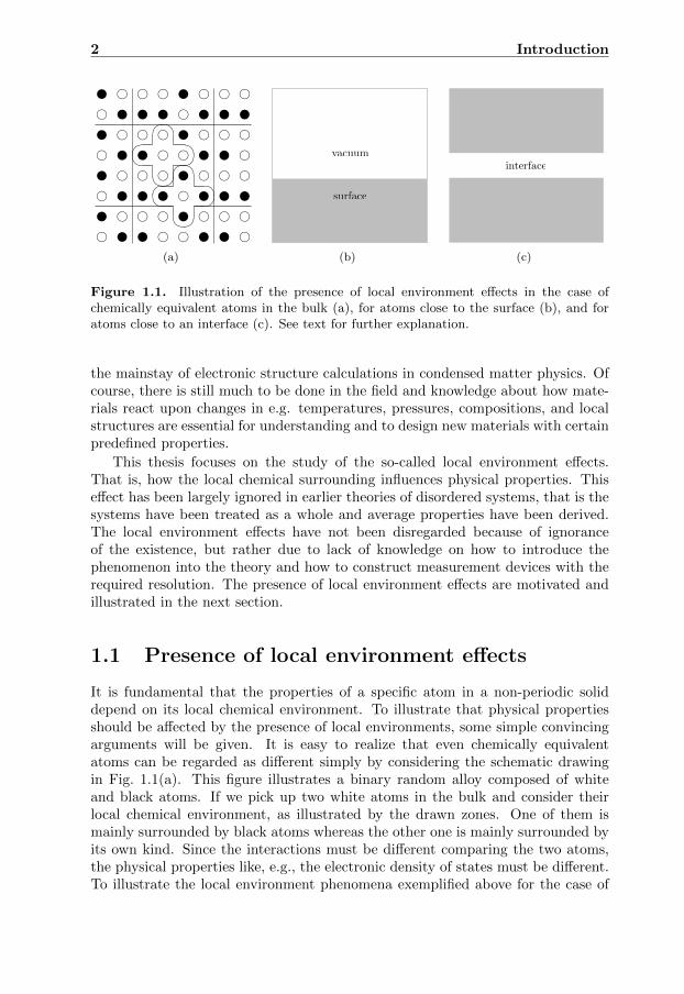
Figure 1.1. Illustration of the presence of local environment effects in the case ofchemically equivalent atoms in the bulk (a), for atoms close to the surface (b), and foratoms close to an interface (c). See text for further explanation.
the mainstay of electronic structure calculations in condensed matter physics. Ofcourse, there is still much to be done in the field and knowledge about how mate-rials react upon changes in e.g. temperatures, pressures, compositions, and localstructures are essential for understanding and to design new materials with certainpredefined properties.
This thesis focuses on the study of the so-called local environment effects.That is, how the local chemical surrounding influences physical properties. Thiseffect has been largely ignored in earlier theories of disordered systems, that is thesystems have been treated as a whole and average properties have been derived.The local environment effects have not been disregarded because of ignoranceof the existence, but rather due to lack of knowledge on how to introduce thephenomenon into the theory and how to construct measurement devices with therequired resolution. The presence of local environment effects are motivated andillustrated in the next section.
1.1 Presence of local environment effects
It is fundamental that the properties of a specific atom in a non-periodic soliddepend on its local chemical environment. To illustrate that physical propertiesshould be affected by the presence of local environments, some simple convincingarguments will be given. It is easy to realize that even chemically equivalentatoms can be regarded as different simply by considering the schematic drawingin Fig. 1.1(a). This figure illustrates a binary random alloy composed of whiteand black atoms. If we pick up two white atoms in the bulk and consider theirlocal chemical environment, as illustrated by the drawn zones. One of them ismainly surrounded by black atoms whereas the other one is mainly surrounded byits own kind. Since the interactions must be different comparing the two atoms,the physical properties like, e.g., the electronic density of states must be different.To illustrate the local environment phenomena exemplified above for the case of

1.1 Presence of local environment effects 3
!7.5 !6.0 !4.5 !3.0 !1.5 0.0 1.5
Ag
Pd
DO
S (
arb
itra
ry u
nits)
E!EF [eV]
2 Pd
3 Pd
4 Pd
5 Pd
6 Pd
7 Pd
8 Pd
9 Pd
10 Pd
2 Ag
3 Ag
4 Ag
5 Ag
6 Ag
7 Ag
8 Ag
9 Ag
10 Ag
Figure 6: Density of states at di!erent Ag and Pd atoms in Ag50Pd50 random alloy as afunction of numbers of atoms of opposite kind in their first coordination shell. The DOS forAg and Pd are shown in the upper and lower part respectively.
Local environment e!ects in random alloys: the density of states.
In this section we illustrate the existence of the local environment e!ects in random alloysby studying the dependence of the density of states at di!erent atoms in random Ag-Pdand Cu-Pd alloys on the number of unlike atoms in their surrounding. In general, theproperties for a specific atom in an alloy depend on its chemical environment [6, 8]. Thesee!ects can be studied within the supercell approach using the LSGF method discussed inthe previous section. The figures below show the density of states (DOS) at di!erent atomsin the equiatomic alloys, which have di!erent number of neighboring atoms of oppositekind. One sees substantial variations of the DOS as one goes from two to ten atoms ofopposite kind in the first coordination shell for the same alloy components. We would liketo remark that these di!erences are observed in completely random alloys: the supercellswere constructed in such a way that short-range order parameters are essentially zeroes upto the sixth coordination shell. We therefore can conclude, that (i) local environment e!ectsdo exist, and (ii) we can capture them by means of our theoretical methodology. However,there are two important questions. Firstly, it is interesting if these e!ects can be observedexperimentally, and, secondly, are there any cases when the local environment e!ects canqualitatively influence physical phenomena. In the next section we will answer the formerquestion.
!7.5 !6.0 !4.5 !3.0 !1.5 0.0 1.5
2 Pd
3 Pd
4 Pd5 Pd
6 Pd
7 Pd
8 Pd9 Pd
10 Pd
Cu
Pd
2 Cu
3 Cu
4 Cu
5 Cu
6 Cu
7 Cu
8 Cu
9 Cu
10 Cu
E!EF [eV]
DO
S (
arb
itra
ry u
nits)
Figure 7: Density of states at di!erent Cu and Pd atoms in Cu50Pd50 random alloy as afunction of numbers of atoms of opposite kind in their first coordination shell. The DOS forCu and Pd are shown in the upper and lower part respectively.
Disorder broadening of core-level photoemission line shapein random metallic alloys
Experimental determination of disorder broadening
Binding energies of core electrons show energy shifts which depend on the chemical environ-ment of the atom. This is why studies of the di!erence between the core electron bindingenergies in the elemental metal and for example in a disordered alloy can help to provide abetter understanding of the electronic structure and the bonding properties of a solid. Thecore level energy shift (CLS) is relatively easy to measure using x-ray photoelectron spec-troscopy, and it was shown to be related to di!erent properties of materials. For example,the shift is shown to be related to the cohesive energy1 [23] and the segregation energy [24].
Of particular interest for us is a study by R. J. Cole et al. [7], where an evidence for”disorder broadening” of core level x-ray photoemission line shapes in alloys was presentedand the broadening was attributed to variations in local properties of alloy components. Theanalysis of the experimental data starts with determination of the instrumental resolution.When this is done the XPS line of the pure metal is investigated. The latter is simulated usingthe Doniach–Sunjic (DS) lineshape2 which is characterized by two parameters, the lifetimeparameter and an assymetry index. The DS lineshape is broadened by a Gaussian to simulatethe instrumental broadening. Numerical fitting then allows determination of the lifetimeparameter and the assymetry index. When investigating the alloy spectra one assumes thatthe lifetime parameter does not change upon alloying. Thus only the assymetry index is a
1The energy that must be added to a crystal to separate its components into free atoms at rest.2See for instance Ref. [25] for a detailed derivation of the function.
E ! EfE ! Ef
DOS(arb.units)
DOS(arb.units)
Ag
Pd Pd
Cu
Figure 1.2. Density of states at different atoms in the equiatomic face-centered cubicAgPd (left panel) and CuPd (right panel) random alloys. The chosen atoms have differentnumber of atoms of opposite kind in their first coordination shell, as indicated by thenumbers to the left in each figure. See Fig. 3.2(c) for an illustration of the fcc crystalstructure.
the bulk, the calculated density of states at different atoms in the equiatomic face-centered cubic (fcc) random AgPd and CuPd alloys are presented, see Fig. 1.2.The atoms are chosen to have different number of atoms of opposite kind in theirfirst coordination shell (nearest neighbors), similar to the schematic in Fig. 1.1(a).A substantial variation of the DOS is seen for the components constituting thealloys when going from two to ten atoms of opposite kind as nearest neighbors,reflecting the presence of local environment effects.
Another example is the presence of surfaces or interfaces, which also leads todifferences in properties between chemically equivalent atoms. In Fig. 1.1(b) asurface is created. For instance, if one considers atoms close to the vacuum theypossess different properties as compared to chemically equivalently atoms in thebulk, due to different chemical environments. The same argument can be used inthe case of an interface in Fig. 1.1(c). Hence, as motivated and shown above, thelocal environment effects do really exist and the available theoretical tools thatwill be presented in the following chapters are able to capture these effects.
The question is if the local environment effects can qualitatively influence phys-ical phenomena. It is within this context the work in this thesis has been done.The overall aim has been to theoretically investigate the effect of local environ-ments on observable physical properties. For instance, the work includes studies ofthe distribution of core-level binding energy shifts as well as Auger shifts in chem-ically disordered bulk metallic alloys. Local environment effects in inhomogeneoussystems are also studied as well as its influence on magnetic properties.

4 Introduction
1.2 Outline of the thesis
The thesis is organized as follows: in Chapter 2 the density-functional theory isintroduced. This is the basic underlying theory that has been used in the calcula-tions. After that follows a chapter that presents different computational techniquesused to solve the electronic structure problem. Chapter 4 deals with different waysto model random alloys. Results are devoted to Chapters 5 through 7. I will alsooverview the theoretical tools that were used to study the specific physical prop-erties in those chapters. After that follows a chapter with conclusions and, at theend, the papers that this thesis is based on are included.

CHAPTER 2
Density-functional theory
2.1 The many-body problem
As mentioned in the introduction, the invention of quantum-mechanics and thederivation of the Schrodinger equation made it possible to describe interactionsat an atomic level. The time-independent version of the Schrodinger equation isgenerally written as
HΨ = EΨ, (2.1)
where Ψ and E correspond to the many-body wave-function and the total energyof the system, respectively. If we consider a system of M nuclei and N electronsthe Hamiltonian H may be decomposed into the following terms1.
H =− 1
2
M∑
i=1
1
Mi∇2Ri− 1
2
N∑
j=1
∇2rj +
1
2
M,M∑
i=1,k=1i6=k
ZiZk|Ri −Rk|
+1
2
N,N∑
j=1,l=1j 6=l
1
|rj − rl|−
M,N∑
i=1,j=1
Zi|Ri − rj |
(2.2)
The first two terms correspond to the kinetic energies of the nuclei and electrons,respectively. The following terms are the electrostatic Coulomb interactions be-tween the nuclei, among the electrons and the last term represents the interactionbetween electrons and nuclei. Moreover, Mi and Zi denote the mass and charge ofthe i:th nucleus. In general the total wave-function is a function of all the spatial
1In Hartree atomic units: ~ = e = me = 4πε0 = 1.
5

6 Density-functional theory
and spin coordinates of the electrons, rj :s and σj :s, and all the spatial coordinatesof the nuclei, Ri:s, that is
Ψ = Ψ(rj , σj ,Ri) where j = 1, . . . , N and i = 1, . . . ,M. (2.3)
The problem with Eq. (2.2), although elegant in its form, is that it is practicallyimpossible to solve for systems containing more than a few atoms. If we considerthe fact that the building blocks of a solid typically consist of 1023 atoms one easilyrealizes that other formulations and/or approximations are needed.
A first attempt to simplify the problem is to consider the mass difference be-tween nuclei and electrons. Since the nuclei are much heavier they will move muchslower than the electrons. Thus, the electronic and ionic degrees of freedom maybe decoupled from each other. The electronic subproblem can be treated as ifthe electrons were moving around in some external potential from the stationarynuclei. If we make use of this so-called Born-Oppenheimer approximation, or adi-abatic approximation, the first term in Eq. (2.2) may be cancelled. Moreover, theterm corresponding to the interactions between the nuclei may be left out sinceit will contribute by constant term, though it has to be considered if the totalenergy is to be calculated. Even though the problem is greatly simplified we stillhave to find the many-body wave-function of the electrons that is a solution tothe reduced Hamiltonian. That is, to find
Ψ = Ψ(rj , σj) where j = 1, . . . , N, (2.4)
an unmanageable problem due to the enormous amount of electrons involved in areal sample. Hence, a reformulation of the problem is necessary.
2.2 The Hohenberg-Kohn theorems
The general idea behind density-functional theory (DFT) is to replace the 3Nspatial degrees of freedom of the electrons by the electron density, that is, onescalar function that only depends on the position in space.
The first approach to use the density as a fundamental variable was proposed byThomas and Fermi [1, 2]. They based their model on the density of a homogeneouselectron gas for the kinetic energy and neglected the exchange and correlationsamong the electrons. It turned out that their approximations were too crude tobe applied and make accurate predictions of materials properties. Inspired bythe approach, Hohenberg and Kohn later formulated DFT as an exact theory ofmany-body systems. Before proceeding one should mention that DFT is a theoryvalid for any correlated many-body system. However, in the following it will bediscussed in the context of interacting electrons subject to the external field, Vext,generated by the nuclei.
Hohenberg and Kohn formulated two theorems that constitute the basis ofmodern DFT [3].
Theorem 1 For any system of interacting particles the external potential Vext(r)is within a constant uniquely determined by the ground state density, n0(r). Thatis, the density may be used instead of the potential to characterize the system.

2.3 The Kohn-Sham scheme 7
Theorem 2 For any external potential, Vext(r), it is possible to define a universalfunctional, F [n(r)], for the total energy functional, E[n(r)]. For a particularexternal potential, the exact ground-state energy is the minimum value of theenergy functional. The density that minimizes the functional is the ground-statedensity, n0(r).
Theorem 1 implies that, given the ground-state density, n0(r), all properties ofthe system is known (since the Hamiltonian is fully determined, except for thetrivial shift in energy). Theorem 2 means that the total energy functional alone issufficient to determine the ground-state density. The proofs of the theorems canbe found in Ref. [4].
The total energy functional can in the Hohenberg and Kohn representation bewritten as
EH-K[n] = F [n] +
∫n(r)Vext(r)dr, (2.5)
where the universal function may be expressed as
F [n] = Te[n] + Vee[n]. (2.6)
The universality of F [n] comes from the independence of the external potential.It contains the kinetic energy Te and the interaction energy Vee of the electrons,functionals that only depend on the density.
2.3 The Kohn-Sham scheme
One year after the groundbreaking theorems that told us that the density couldbe used as a fundamental variable, Kohn and Sham proposed an anzats on how tosolve the equations in practice. The main idea in the Kohn-Sham anzats [5] is toreplace the many-body problem, Eqs. (2.1) and (2.2), by an auxiliary independent-particle problem and incorporate all many-body effects in the so-called exchange-correlation energy functional. This fictitious system has the constraint to yieldthe same ground-state density as the physical system.
The kinetic energy for non-interacting electrons can be evaluated exactly as
Ts[n] = −1
2
N∑
j
〈φj |∇2|φj〉, (2.7)
where φj are the one-particle orbitals which in turn are solutions to the Schrodingerlike equation, the so-called Kohn-Sham equation
(− 1
2∇2 + veff(r)
)φj(r) = εjφj(r), (2.8)
with energy-eigenvalues εj . The ground-state density is calculated from the one-particle orbitals
n(r) =
N∑
j
|φj(r)|2, (2.9)

8 Density-functional theory
where the sum is over the N lowest occupied states.Within the Kohn-Sham approach the energy functional is written as [5]
EK-S[n] = Ts[n] +
∫n(r)Vext(r)dr +
1
2
∫∫n(r)n(r′)
|r − r′| drdr′ + Exc[n]. (2.10)
The second term in the equation above represents the density interacting with theexternal potential, the third term is the electrostatic self-interaction energy of thedensity, known as the Hartree energy, and the last term denotes the exchange-correlation energy. If one compares EH-K[n] and EK-S[n], that is Eqs. (2.5) and(2.10), the Exc[n] is defined as
Exc[n] =(Te[n]− Ts[n]
)+(Vee[n]− 1
2
∫∫n(r)n′(r)
|r − r′| drdr′). (2.11)
Thus, Exc[n] is the difference in the kinetic and the internal interaction energies ofthe physical many-body system and the non-interacting auxiliary system, wherein the fictitious system the interactions among the electrons are replaced by theHartree energy.
Now we seek to find an expression for the effective potential veff entering theKohn-Sham equation (2.8). Let us consider the variation of the interacting andnon-interacting energy functionals with respect to the density. From Eq. (2.10) itfollows that
0 =δ
δn
(EK-S − µ
∫n(r)dr
)
=δTs[n]
δn+ Vext(r) +
∫n(r′)
|r − r′|dr′ +
δExc[n]
δn− µ, (2.12)
where the Lagrange multiplier µ is introduced to satisfy the constraint that thedensity should integrate to the total number of electrons (N=
∫n(r)dr). On the
other hand for non-interacting electrons moving in the effective potential veff itfollows that
0 =δ
δn
(E[n]− µ
∫n(r)dr
)
=δ
δn
(Ts[n] +
∫n(r)veff(r)dr − µ
∫n(r)dr
)
=δTs[n]
δn+ veff(r)− µ. (2.13)
Using the anzats that the equations are solved for the same density we can simplyidentify the effective potential as
veff(r) = Vext(r) +
∫n(r′)
|r − r′|dr′ +
δExc[n]
δn. (2.14)
Equations (2.8), (2.9) and (2.14) are known as the Kohn-Sham equations and arecoupled through the density and have to be solved in a self-consistent manner.
2.4 Exchange-correlation functionals 9
Before continuing it is fruitful to study some of the implications of the approach.Starting with the Kohn-Sham equation (2.8) it is easily shown that
N∑
j
εj =
N∑
j
(〈φj | −
1
2∇2 + veff(r)|φj〉
)= Ts[n] +
∫veff(r)n(r)dr, (2.15)
or equivalently
Ts[n] =
N∑
j
εj −∫veff(r)n(r)dr. (2.16)
Substituting this form of Ts[n] into Eq. (2.10) and explicitly write out the expres-sion of veff we can, after some mathematics, write the total energy as
EK-S[n] =
N∑
j
εj −1
2
∫∫n(r)n(r′)
|r − r′| drdr′ −∫δExc[n]
δnn(r)dr + Exc[n]. (2.17)
Here we notice that the total energy is not just the sum over the Kohn-Shamenergy-eigenvalues. Due to their construction they do not represent real particlesand have, in principle, no physical meaning other than producing the correctground-state density. Since the Kohn-Sham eigenvalues are independent particleeigenvalues they do not in general correspond to the true energies for removal ofan electron of the system, nor do the eigenvalue differences provide the correctenergy for neutral excitations [4]. The subject in Papers I–V is about bindingenergy shifts of core electrons, which is related to this part. This will be discussedin Chapter 5.
To sum up, the approach by Kohn and Sham lets us replace the complicatedmany-body problem by an independent particle equation that is much easier tosolve. Thus, the outlined scheme provides a way on how to find the exact ground-state density and ground-state energy of a many-body problem in an independentparticle framework. However, we are left by the unknown functional Exc[n] whichhas to be approximated in some manner. Before going into this discussion oneshould note that the contribution from this term is rather small as compared tothe other terms contributing to the total energy. Still, it is large enough to be ofimportance for describing physical properties of condensed matter, such as bondingand bulk modulus, etc.
2.4 Exchange-correlation functionals
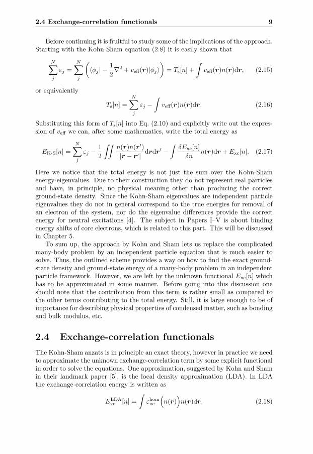
The Kohn-Sham anzats is in principle an exact theory, however in practice we needto approximate the unknown exchange-correlation term by some explicit functionalin order to solve the equations. One approximation, suggested by Kohn and Shamin their landmark paper [5], is the local density approximation (LDA). In LDAthe exchange-correlation energy is written as
ELDAxc [n] =
∫εhom
xc
(n(r)
)n(r)dr. (2.18)

10 Density-functional theory
That is, the exchange-correlation energy at each point in space is approximatedas the product of the density at that point and the exchange-correlation energydensity of an homogeneous electron gas, εhom
xc (n), with that density. The latter isknown from quantum Monte Carlo simulations by Ceperley and Alder [6]. Somecommonly used analytical parameterizations of the data can be found in Refs. [6,7, 8, 9, 10].
Even though the LDA is built to be valid for slowly varying densities it hasproven to perform well even for highly inhomogeneous systems, especially in solidstate physics, and is still frequently used in DFT simulations. One explanationto this success is that in solids the region outside the nuclei, i.e. the interstitialregion mainly responsible for the bonding, the density gradients are rather low.Moreover, it is possible to define a so-called exchange-correlation hole density,which describes the inter-electronic repulsion. An electron present at a point rreduces the probability of finding another electron at r′. It turns out that it is thespherical average of the exchange-correlation hole density that enters the exchange-correlation energy. Thus, even though LDA does not give the right form of theexchange-correlation hole the spherical average is still close to the real one. [7]
Throughout this chapter the spin-dependency has been left out to keep equa-tions more transparent and outline general ideas rather than details. However,all results above can be generalized to account for spin-polarized situations. Ageneralization of the LDA to account for spin-polarization was derived by vonBarth and Hedin [11], the so-called local-spin density approximation (LSDA). Inthis case the exchange-correlation energy density is a function of two spin densitiesεhom
xc (n↑, n↓).The natural step to go beyond the LDA is to include the gradient of the density.
This class has been named the generalized gradient approximation (GGA). Theexchange-correlation energy may be written as [4]
EGGAxc [n↑, n↓] =
∫εGGA
xc
(n↑(r), n↓(r), |∇n↑(r)|, |∇n↓(r)|
)n(r). (2.19)
There are different forms of the GGA available, some commonly used functionalsare found in Refs. [12, 13, 14, 15].
Naturally, GGAs are better than LDAs in describing atoms and moleculessince quite substantial gradient dependency is involved. Usually, LDA also un-derestimates the lattice spacing for the 3d series of the transition metals. Due tothis underestimation, LDA for instance fails to correctly predict ferromagnetic Feto have bcc as ground-state crystal structure, while GGA does not. Equal per-formance is generally obtained for the ground-state properties of the 4d metals,whereas for the 5d metals LDA is usually better. [16]
CHAPTER 3
Solving the Kohn-Sham equations
3.1 Computational scheme
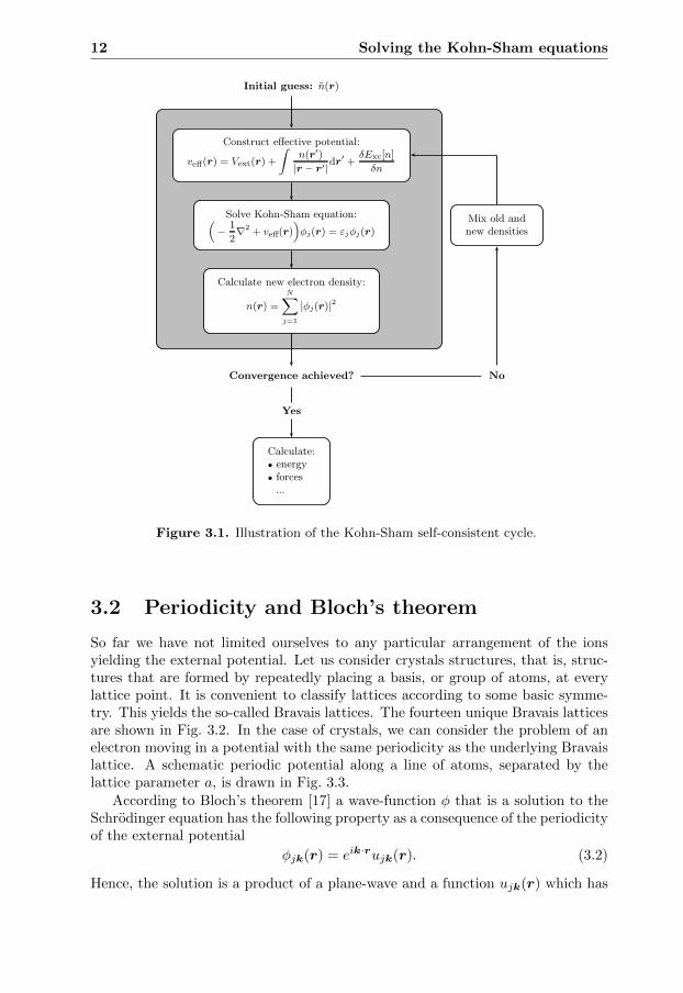
The Kohn-Sham equations provide a method for finding the exact ground-statedensity. In practice we need to solve these equations numerically in a self-consistentway since they are coupled through the density. The procedure is schematicallygiven in Fig. 3.1. The shaded area represents the key equations in the Kohn-Shamscheme. Actual calculations start with an initial guess of the density, a so-calledtrial density n(r). With this density we can construct and calculate the effectivepotential, which in turn is used in the Kohn-Sham equation. The solution tothe one-electron eigenvalue problem gives a new density. A comparison to theprevious density can be used as a self-consistently criterion. Successive changes ofthe density are made until a self-consistent solution is found. Once it is reached,ground-state properties can be calculated.
In general, to solve the Kohn-Sham equations the wave-functions have to beexpanded in some basis-set
|φj〉 =∑
i
αi|ξi〉, (3.1)
where α and |ξ〉 denote the expansion coefficients and basis functions, respectively.
There exists different methods for solving the Kohn-Sham equation, each hav-ing its advantages and disadvantages. An overview of some of the methods willbe presented in the following sections. First, we will have a look at the transla-tional symmetry that crystals possess and how it can be utilized to reduce thecomputational cost.
11
12 Solving the Kohn-Sham equations
Initial guess: n(r)
Construct effective potential:
veff(r) = Vext(r) +
∫
n(r′)
|r − r′|dr′ +
δExc[n]
δn
Solve Kohn-Sham equation:(
−1
2∇2 + veff(r)
)
φj(r) = εjφj(r)Mix old andnew densities
Calculate new electron density:
n(r) =
N∑
j=1
|φj(r)|2
Convergence achieved? No
Yes
Calculate:• energy• forces...
Figure 3.1. Illustration of the Kohn-Sham self-consistent cycle.
3.2 Periodicity and Bloch’s theorem
So far we have not limited ourselves to any particular arrangement of the ionsyielding the external potential. Let us consider crystals structures, that is, struc-tures that are formed by repeatedly placing a basis, or group of atoms, at everylattice point. It is convenient to classify lattices according to some basic symme-try. This yields the so-called Bravais lattices. The fourteen unique Bravais latticesare shown in Fig. 3.2. In the case of crystals, we can consider the problem of anelectron moving in a potential with the same periodicity as the underlying Bravaislattice. A schematic periodic potential along a line of atoms, separated by thelattice parameter a, is drawn in Fig. 3.3.
According to Bloch’s theorem [17] a wave-function φ that is a solution to theSchrodinger equation has the following property as a consequence of the periodicityof the external potential
φjk(r) = eik·rujk(r). (3.2)
Hence, the solution is a product of a plane-wave and a function ujk(r) which has

3.2 Periodicity and Bloch’s theorem 13
I. Cubic
(a) Simple (b) Body-centered (c) Face-centered
II. Orthorhombic
(d) Simple (e) Body-centered (f) Face-centered (g) Base-centered
III. Monoclinic IV. Tetragonal
(h) Simple (i) Base-centered (j) Simple (k) Body-centered
lV. Hexagonal VI. Trigonal (Rhombohedral) VII. Triclinic
(l) Hexagonal (m) Trigonal (n) Triclinic
Figure 3.2. Bravais lattices grouped into the seven crystal systems. The ai:s are thebasis vectors that span the unit cell.
the property of having the same periodicity as the potential (lattice). Since
V (r) = V (r + T ) (3.3)
with T = n1a1 + n2a2 + n3a3 being a translation vector and a:s Bravais latticevectors, it follows from the theorem that
ujk(r) = ujk(r + T ), (3.4)
which allow us to write an equivalent form of Bloch’s theorem
φjk(r + T ) = eik·Tφjk(r). (3.5)
The proof of the theorem can be found in Refs. [4, 18].

14 Solving the Kohn-Sham equationssnoitauqemahS-nhoKehtgnivloS41
a
V(x)
x
Figure 3.3. A schematic crystalline periodic potential V (x ) along a line o! ons, sepa-rated by the lattice parameter a . The equilibrium ion sites are marked with !lled graycircles. The shaded area corresponds to one particular choice of unit cell.
a
x
V (x)
Figure 3.3. A schematic crystalline periodic potential V (x) along a line of ions, sepa-rated by the lattice parameter a. The equilibrium ion sites are marked with filled graycircles. The shaded area corresponds to one particular choice of unit cell.
The result of Bloch’s theorem is that the electronic structure problem of a solidis significantly simplified, since it is only necessary to solve the Schrodinger equa-tion, or Kohn-Sham equation, for one unit cell (or supercell as will be introducedlater). In the one-dimensional case one may choose the space which corresponds tothe shaded area in Fig. 3.3. In the reciprocal space this corresponds to consideringthe electrons contained in the first Brillouin zone (BZ). Moreover, in addition totranslational symmetry, crystals may also exhibit symmetries under rotation andinversion. This further reduces the space where we have to solve the equations,since certain wave-vectors inside the BZ become equivalent. The smallest possiblepart in reciprocal space that contains a complete set of inequivalent k-vectors iscalled the irreducible part.
3.3 Plane-wave expansion technique
One common method to expand the wave-function is to use plane-waves. Theperiodic part of Eq. (3.2) can be Fourier expanded as
ujk(r) =∑
G
cjk,GeiG·r, (3.6)
where the summation is over reciprocal lattice vectors G, and cjk,G are the expan-sion coefficients. Thus, the orbitals for the independent electrons may be expressedas
φjk(r) =∑
G
cjk,Gei(G+k)·r. (3.7)
3.3 Plane-wave expansion technique 15
The periodic potential in a crystal may also be expressed as a sum of Fourier com-ponents in the same way as the wave-function above. Inserting the Fourier trans-form of the wave-function and the potential into the Kohn-Sham equation (2.8),and using the orthonormality of plane-waves, the equation can be rewritten in amatrix form and the eigenfunctions cjk,G with corresponding energy-eigenvaluesεjk can be found through diagonalization. [4]
An advantage of using plane-wave basis set is that it is straightforward tocalculate forces and hence to obtain relaxed geometries, due to their explicit inde-pendence of atomic positions [4]. It is also easy to control the basis set convergenceby increasing the cut-off energy in the Fourier expansion. In practical calculationsthe expansion of the wave-functions is truncated by only keeping plane-waves with
a kinetic energy lower than a specified cut-off value, that is ~2
2m |k +G|2 < Ecut.
However, a problem arises in the vicinity of the core regions of atoms. In thisregion the electronic wave-functions oscillate rapidly due to the strong Coulombinteraction with the nuclei together with Pauli exclusion principle. This makethem a lot harder to describe and prohibitively many plane-waves are required inthe expansion.
An approach to circumvent this problem is to introduce pseudopotentials. Thegeneral idea behind the approach is that the core states are localized and do notparticipate in the bonding as the valence states do. Then, one can assume thatthe core electron distribution is the same irrespective of the chemical environmentsurrounding the atom. This is referred to as the frozen core approximation. Thus,the core states can be assumed to be fixed and need to be calculated once for asingle isolated atom (or another chosen reference system). In doing so one alsodecreases the computational effort, since only the valence electrons have to beconsidered in the calculations.
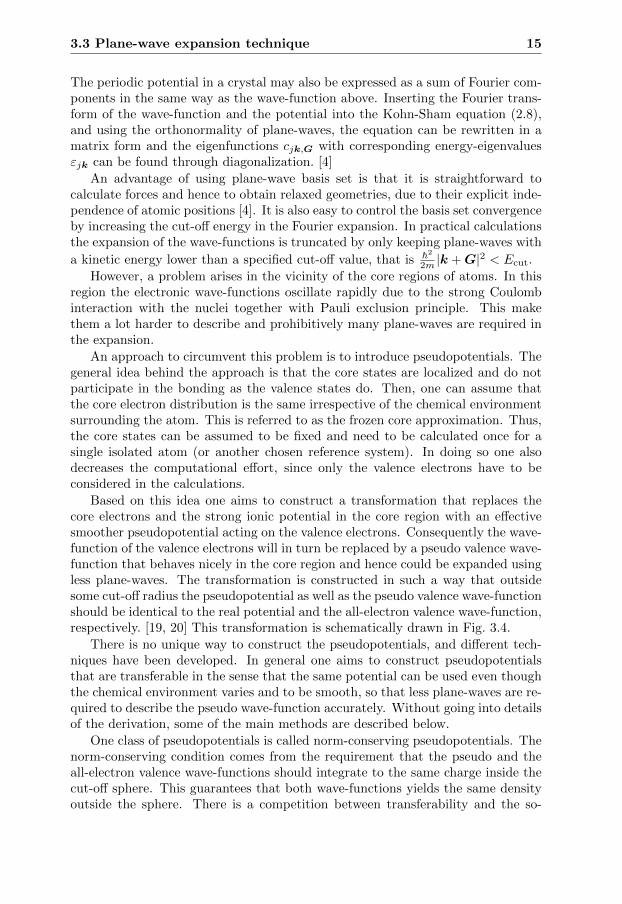
Based on this idea one aims to construct a transformation that replaces thecore electrons and the strong ionic potential in the core region with an effectivesmoother pseudopotential acting on the valence electrons. Consequently the wave-function of the valence electrons will in turn be replaced by a pseudo valence wave-function that behaves nicely in the core region and hence could be expanded usingless plane-waves. The transformation is constructed in such a way that outsidesome cut-off radius the pseudopotential as well as the pseudo valence wave-functionshould be identical to the real potential and the all-electron valence wave-function,respectively. [19, 20] This transformation is schematically drawn in Fig. 3.4.
There is no unique way to construct the pseudopotentials, and different tech-niques have been developed. In general one aims to construct pseudopotentialsthat are transferable in the sense that the same potential can be used even thoughthe chemical environment varies and to be smooth, so that less plane-waves are re-quired to describe the pseudo wave-function accurately. Without going into detailsof the derivation, some of the main methods are described below.
One class of pseudopotentials is called norm-conserving pseudopotentials. Thenorm-conserving condition comes from the requirement that the pseudo and theall-electron valence wave-functions should integrate to the same charge inside thecut-off sphere. This guarantees that both wave-functions yields the same densityoutside the sphere. There is a competition between transferability and the so-

16 Solving the Kohn-Sham equations
! "Z
r
rcut r
V PP
!PP
!AE
Figure 3.4. Illustration of the transformation of the strong Coulomb potential of thenucleus (—) to the pseudopotential V PP (···) and the corresponding transformation ofthe all-electron wave-function ψAE (—) to the pseudo wave-function ψPP (···). At thecut-off radius rcut it is required that the corresponding quantities match each other.
called softness of the pseudo-functions in terms of the number of plane-waves thatis required to expand the wave-function. In general, to have a high transferabilityone should, of course, minimize rcut to resemble more of the real potential. Onthe other hand for larger cut-off radius the pseudopotentials become softer andless plane-waves are needed. [4]
Another family of pseudopotentials widely used in the condensed matter com-munity was proposed by Vanderbilt, the so-called ultrasoft pseudopotentials [20].In order to have such soft pseudopotentials the norm-conserving condition is re-leased. The price to pay to achieve these properties and yet being accurate isthat equation becomes much more complex. For instance augmentation chargeshave to be introduced due to the deficit in the core region [20]. Nevertheless,the use of ultrasoft pseudopotentials is usually more advantageous than the norm-conserving pseudopotentials considering the gain in computational cost. However,the drawback with the above methods is that in the transformation to smoothwave-functions the information about the all-electron wave-function close to thenuclei is lost.
At last, another important method to solve electronic structure problem is theall-electron projector-augmented wave method (PAW), proposed by Blochl [21].Similar to the pseudopotential methods a transformation to smooth wave-functionsis done to address the problem of rapid oscillations of the wave-functions in thevicinity of the nuclei. However, in the PAW method the true all-electron wave-function and hence electronic density is retained. This is achieved by a linear

3.4 Green’s function technique 17
transformation that couples the true wave-functions to smooth auxiliary wave-functions, that are much more numerically convenient. Since the wave-functionsalready are smooth at some distance from the nuclei the transformation shouldonly modify the wave-functions in some sphere centered around the nuclei. Outsidethis sphere the transformation is unity. Finding such a transformation enables oneto expand the auxiliary wave-functions in a convenient basis-set in the core regionand then reconstruct the true wave-function and density. This enables calculationof physical properties that require knowledge about the electron density close tothe nuclei [22].
For further reading and details about the methods see Refs. [4, 20, 21, 23] andreferences therein.
In this thesis two electronic structure programs that utilizes the pseudopo-tential and the PAW approach have been used, the Vienna Ab initio SimulationPackage (vasp) [23, 24, 25] and the Quantum opEn Source Package for Researchin Electronic Structure, Simulation, and Optimization (quantum-espresso) [26].
3.4 Green’s function technique
Another approach to solve the Kohn-Sham equation is the Green’s function tech-nique. An advantage with this method is that it is suitable and straightforwardto extend the formalism to treat disorder and to handle defects without having toconstruct large supercells. The theory of disordered systems will be the subjectof the next chapter. For ordered system though, the wave-function methods areusually computationally more efficient.
The one-particle Green’s function G(r, r′, E) that describes the propagation ofan independent electron with energy E from r to r′ is defined as the solution tothe equation
(− 1
2∇2 + veff(r)− E
)G(r, r′, E) = −δ(r − r′). (3.8)
It may also be found through the one-particle wave-functions that are solutions tothe Kohn-Sham equation (2.8).
G(r, r′, E + iξ) =∑
j
φj(E, r)φ∗j (E, r′)
E + iξ − εj(3.9)
This is known as the spectral representation and the poles give the eigenenergiesto the Hamiltonian. Given the Green’s function various physical properties canbe derived, e.g. the electron density per spin
n(r) = − 1
π
EF∫Im[G(r, r, E)]dE (3.10)
and the density of states
n(E) = − 1
π
∫
V
Im[G(r, r, E)]dr. (3.11)

18 Solving the Kohn-Sham equations
!"#$!"#$
!"#$!"#$
!"#$
!"#$
!"#$
!"#$
!"#$
!!"V (r)
VMTZ
S
Figure 3.5. Schematic drawing of the muffin-tin potential is shown to the left. The righthand part shows a top view of the potential landscape. The landscape is divided intotwo type of regions, the interstitial region with a flat potential, VMTZ, and the regionswithin a sphere, defined by the radius S, with a spherically symmetric potential, V (r).
Even though the Green’s function formally may be found through the Kohn-Shamorbitals there exists a more efficient and natural formalism. This method is knownas the Korringa-Kohn-Rostocker (KKR) method or the multiple-scattering the-ory [27, 28].
The main idea of the multiple scattering theory is to treat all atoms as scatter-ing centers and to find a solution to the electronic structure problem by demandingthat the incident wave at each scattering center equals the sum of the outgoingwaves from all other scattering centers. Although no restriction on the potentialhas to be done, the so-called muffin-tin (MT) potentials proposed by Slater [29]may be used. The effective potential that enters the Kohn-Sham equations is thenassumed to be spherically symmetric inside the MT sphere centered around eachnucleus and constant in the interstitial region. That is, we may write the potentialas
VMT(r) =
{V (r) r 6 SVMTZ = const. r > S
, (3.12)
where S defines the radius of the MT sphere, V (r) and VMTZ denote the sphericallyaveraged crystal potential and the muffin-tin zero, respectively. In this way eachsite can be viewed as a spherical scatterer. A schematic figure of the MT potentialis given in Fig. 3.5.
Following the example in Ref. [16] and considering the MT spheres to be non-overlapping the solution to the scattering problem may be written as
G(r +Ri, r′ +Rj , E) =
∑
LL′
Ril(r, E)gijLL′(E)Rjl′(r′, E)
− δij∑
L
Ril(r, E)Hjl(r′, E). (3.13)
The vectors r and r′ denote the coordinates within the spheres centered at Ri
and Rj , respectively. Ril and Hil represent the regular and irregular solutions tothe Schrodinger equation inside a MT sphere centered at site i for orbital angular

3.4 Green’s function technique 19
momentum l and energy E (measured relative to the VMTZ). The sum is over allL, representing the combined angular momentum quantum numbers (l,m). Thescattering path operator gijLL′(E) appearing in the equation above is an importantquantity that describes the propagation of a state between sites i and j. In asimple one-component crystal the scattering path operator is given by [16]
gijLL′ =1
VBZ
∫
BZ
[m(E)−B(k, E)]−1LL′e
ik(Ri−Rj)dk, (3.14)
where the integration is over the Brillouin zone. Here m(E) is defined as thepotential function matrix and B(k, E) is the Fourier transform of the structureconstant matrix. Although we have made simplifications above, the separationof the potential part from the structure part is a general feature of the multiplescattering formalism and is advantageous when dealing with disordered systems [4,16], as will be further discussed in the next chapter.

20 Solving the Kohn-Sham equations

CHAPTER 4
Electronic structure of random alloys
4.1 Introduction
So far we have assumed that we have the translational symmetry of a Bravaislattice. However, when alloys are created, it is common that solid solutions areformed that lack any long-range periodicity in the distribution of the components.In such cases the translational symmetry breaks down. This substitutional disor-der differ from so-called topological disorder, the situation in liquids and amor-phous systems, since it is still possible on the average to associate atoms to latticepositions.
When modelling solid solutions, without the knowledge on how alloy compo-nents are distributed on the lattice, the completely random alloy is often a goodstarting point. In a completely random alloy, the occupation of the sites by dif-ferent types of atoms is uncorrelated [16].
Due to the lack of long-range order, and particularly in the case of the randomalloy, each ion is placed in a unique local environment and is strictly speakingdifferent from all other atoms in the crystal. It is a real challenge to model thesekind of systems using first-principles methods.
4.2 Supercell approach
One approach to deal with the problem of lost translational symmetry is to usethe concept of supercells. A supercell is a large cell created by repeating theprimitive unit cell a certain number of times in each direction in space. In thisway several lattice sites are generated on which atoms can be distributed in adesired way. Of course, also the supercell obey periodic boundary conditions andthus translational symmetry but with the possibility to introduce different local
21

22 Electronic structure of random alloys
!"!"!"!"
"!"!"!"!
"!"!"!"!
"!"!"!"!
!"!"!"!"
"!"!"!"!
"!"!"!"!
"!"!"!"! Figure 4.1. An illustration of a two-
dimensional supercell that is repeatedperiodically through space.
chemical environments. This is schematically illustrated in Fig. 4.1. The problemis how the atoms should be placed on the lattice sites of the supercell in order tomimic the random alloy in the best way. One obvious way would be to use hugesupercells and then distribute alloy components using a random number generationscheme. Unfortunately such schemes turn out to be rather cumbersome in practicesince very large cells are needed to obtain accurate results. Improvements basedon averaging over several different supercells are also computationally demanding.
Another approach to this problem was suggested by Zunger et al. when intro-ducing the so-called special quasi-random structure (SQS) method [30]. Withinthis approach it is possible to only consider one configuration of atoms by con-structing a smart supercell instead of just generate large ones by random numbergenerators. To answer the requirements of what criteria such a smart supercellshould fulfill, one needs to cluster expand the configurational part of the totalenergy of an alloy.
Sanches et al. [31] derived a formalism for describing configurational clusterfunctions in a system containing arbitrarily number of components. For instanceconsider M components that occupy N lattice points, then any of the MN con-figurations are characterized by the vector σ=(σ1, . . . , σN ). The spin occupationvariable σi takes on values ±(m,m − 1, . . . , 1(0)) for an M = 2m(2m + 1) com-ponent system. The numbers within brackets refer to the case when odd numberof components are considered. What we need to find is a set of functions thatspan the configurational space. For simplicity, to outline the general idea, let usconsider a system of M = 2 components, i.e. an AB alloy, with N lattice points.In this case the spin occupation number σi takes the value +1 if site i is occupiedby the A component and −1 if occupied by an B atom. Consider site i, it is easilyshown that the polynomials φ0(σi) = 1 and φ1(σi) = σi form a complete andorthonormal set in the one-dimensional configuration space (point clusters) withthe inner product between two functions of configurations f(σi) and g(σi) definedas
〈f(σi) · g(σi)〉 =1
2
∑
σi=±1
f(σi)g(σi). (4.1)
4.2 Supercell approach 23
(a)
!...
!!
!...
!!
!...
!!
!...
!!
!...
!!"#
i1 i2 i3
in!1
in
(b)
!...
!!
!...
!!
!...
!!
!...
!!
!...
!!
j1 j2 j3
jn!1
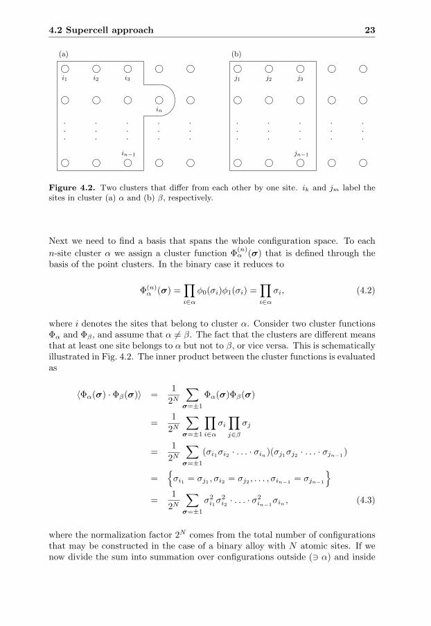
Figure 4.2. Two clusters that differ from each other by one site. ik and jm label thesites in cluster (a) α and (b) β, respectively.
Next we need to find a basis that spans the whole configuration space. To each
n-site cluster α we assign a cluster function Φ(n)α (σ) that is defined through the
basis of the point clusters. In the binary case it reduces to
Φ(n)α (σ) =
∏
i∈αφ0(σi)φ1(σi) =
∏
i∈ασi, (4.2)
where i denotes the sites that belong to cluster α. Consider two cluster functionsΦα and Φβ , and assume that α 6= β. The fact that the clusters are different meansthat at least one site belongs to α but not to β, or vice versa. This is schematicallyillustrated in Fig. 4.2. The inner product between the cluster functions is evaluatedas
〈Φα(σ) · Φβ(σ)〉 =1
2N
∑
σ=±1
Φα(σ)Φβ(σ)
=1
2N
∑
σ=±1
∏
i∈ασi∏
j∈β
σj
=1
2N
∑
σ=±1
(σi1σi2 · . . . · σin)(σj1σj2 · . . . · σjn−1)
={σi1 = σj1 , σi2 = σj2 , . . . , σin−1
= σjn−1
}
=1
2N
∑
σ=±1
σ2i1σ
2i2 · . . . · σ2
in−1σin , (4.3)
where the normalization factor 2N comes from the total number of configurationsthat may be constructed in the case of a binary alloy with N atomic sites. If wenow divide the sum into summation over configurations outside (3 α) and inside

24 Electronic structure of random alloys
(∈ α) α we may rewrite the above expression as
〈Φα(σ) · Φβ(σ)〉 =1
2N
∑
σ=±1︸ ︷︷ ︸3α
·∑
σ=±1︸ ︷︷ ︸∈α
σ2i1σ
2i2 · . . . · σ2
in−1σin
=1
2N2N−n
∑
σi1=±1
σ2i1
∑
σi2=±1
σ2i2 · . . . ·
∑
σin−1=±1
σ2in−1
∑
σin=±1
σin
=1
2n2n−1
∑
σin=±1
σin
=1
2
∑
σin=±1
σin
= 0. (4.4)
Hence, the cluster functions are orthogonal. Following the same scheme as outlinedabove one can show that they are properly normalized, that is 〈ΦαΦβ〉 = δαβ . Itis also possible to show that the completeness relation holds [31]
∑
α
Φα(σ)Φα(σ′) = δ(σ, σ′). (4.5)
Thus, the functions Φα(σ) form a complete orthonormal set in the configurationalspace. This means that any property χ that is a function of configuration may beexpanded in this basis
χ(σ) =∑
α
χ(n)α Φ(n)
α (σ). (4.6)
The expansion coefficients are given by the projections of the function onto thecluster functions
χ(n)α = 〈χ(σ)Φ(n)
α (σ)〉. (4.7)
The space group symmetries of the crystal require that χ(n)α are the same for
clusters that are related by symmetry operations. Accordingly, an alternative wayto write Eq. (4.6) is to introduce the correlation function, ξ(n), for the n-site cluster
α as the average value of the cluster function, ξ(n)f =〈Φ(n)
f 〉, and sum over all figuresf instead of over all clusters [16]
χ(σ) =∑
f
χ(n)f ξ
(n)f . (4.8)
The meaning of a figure is illustrated in Fig. 4.3, where different examples of figuresare drawn for the case of a bcc underlying lattice.
Considering the expansion of the configurational part of the total energy, the
coefficients, V(n)f , are called effective cluster interactions (ECIs) and may be writ-
ten asEconf(σ) =
∑
f
V(n)f ξ
(n)f . (4.9)

4.3 Effective medium approach 25
b b
b b
b
b
b
bb
b
bb
b
b
b
b
bb
b
Figure 4.3. Illustrating different figures for the case of a bcc lattice. Examples of apair, a triplet and a tetrahedron are shown from the left to the right.
From Eq. (4.9) we may draw some conclusion on how the supercell should beconstructed in order to mimic the disorder of the random alloy. First one maynotice that the only contribution to the energy comes from the clusters with non-
zero V(n)f . Thus, in order to mimic the random alloy the supercell should be
constructed in such a way that the correlation function ξ(n)f for the terms with
non-zero effective interactions resembles the correlation function for the randomalloy. Ideally one should do so for as many clusters as possible. Of course itcan not be fulfilled for all distant clusters using a finite supercell. However, theinteractions among nearest neighbors are generally more important than distantneighbors. Thus, one should try to exactly match the correlation functions of arandom alloy between the first few nearest neighbor pairs.
4.3 Effective medium approach
Another approach to recover spatial homogeneity in a crystal is the concept ofeffective medium. Instead of direct calculations on supercells one tries to averageout the disorder. The most straightforward way to construct an effective mediummay be to put the average atomic potential on each lattice site, taken with theweight of concentration of the atoms constituting the alloy. This attempt is calledthe virtual crystal approximation. Although it is a nice idea the approximation isoften too simple to be used for prediction of properties of real materials. [32]
Another improved methodology was put forward by Soven in 1967, the so-called coherent potential approximation (CPA) [33], later also implemented in theKKR framework by Gyorffy [34]. The CPA requirement yields that if an electronis propagating through the coherent potential it should on the average be scatteredas it would in the real alloy. The effective potential is put on every lattice pointexcept for the central one where the real potential for one alloy component isplaced (illustrated in Fig. 2 and 3 on pp. 102–103). By doing so the problem can

26 Electronic structure of random alloys
be viewed as a single-impurity placed in an otherwise ideal crystal. One of themain advantages with the KKR Green’s function technique is that it is suitablefor perturbation theory. Suppose the coherent Green’s function g for the effectivepotential m is known, then the on-site scattering path operators gi for each alloycomponent i can be determined through the Dyson equation, that is
gi = g + g(m−mi)gi. (4.10)
The on-site coherent scattering path operator may be determined from the multiplescattering equation introduced in Section 3.4
g =1
VBZ
∫
BZ
dk
m−B . (4.11)
By the definition of CPA it should also be the average of the alloy componentswith concentration ci
g =∑
i
cigi where∑
i
ci = 1. (4.12)
Equations (4.10)–(4.12) form a self-consistent set of equations and can be solvedin an iterative manner. From the knowledge of the scattering path operators ofthe components one can derive physical properties, e.g. the density is given byinserting gi in Eq. (3.13) and then use the result in Eq. (3.10).
The CPA usually works well to describe average properties and is computa-tionally very fast compared to supercell methods. An application of CPA is themodelling of paramagnetic states. That is, states where the magnetic momentsare randomly oriented with zero net magnetic moment. The technique is calledthe disordered local moments method [35] and a simulation is simply carried outby treating the disorder as an equiatomic alloy constituting of spin-up as well asspin-down moments.
However, due to the fact that the CPA is a single-site approximation the theoryhas some embedded shortcomings. The uniqueness of each atom is totally absentsince only the central atom is put into the effective medium, that is each site hasthe same neighborhood. One implication of this is the inability to account forinhomogeneous lattice distortions, see Section 4.5. Another concern is the chargetransfer effects present in real alloys. In CPA the effective medium has to be chargeneutral leading to zero charge transfer and hence the electrostatic interactions cannot be treated. All information about charge transfer lies beyond the single-siteapproximation since information about the local chemical surrounding is required.However, a model to correct for this mistreatment has been proposed, the so-calledscreened impurity model (SIM) [36, 37, 38].
Different implementations that utilize the CPA-Green’s function techniquehave been used in this work. The Bulk Green’s Function Method (BGFM) [39, 40]utilizes the CPA and has for instance been used in Paper VII to extract effectivecluster interactions that are used in Monte Carlo simulations to study the con-centration profile of AgPd thin-films on top of a Ru substrate, see Section 7.1.
4.4 A combined supercell and effective medium method 27
Another method that have been used extensively is the Locally Self-consistentGreen’s Function method (LSGF) [41, 42]. The LSGF method is an approach tocombine the CPA and the supercell approach and go beyond the single-site ap-proximation, as will be evident in the next section when the method is furtherdiscussed. This method has for instance been used in Papers I–III and in Paper Vto study the effect of local chemical environments on core-level shifts and Augershifts, which is the subject in Chapter 5.
In both the LSGF and the BGFM the atomic sphere approximation (ASA) isutilized to describe the potential. Within the ASA the potential is approximatedby MT spheres that have the same volume as the Wigner-Seitz cell. This causesoverlap between neighboring spheres, which makes the scheme to usually performwell for close packed systems [4]. A modification to improve ASA has been de-veloped to not only consider the spherical contribution to the potential but alsoaccount for multipole moments, the so-called ASA+M technique [40, 43].
Another approach worth mentioning here is the Exact Muffin-Tin Orbital(EMTO) method [44]. The EMTO method goes beyond the ASA and describesmore accurately the exact crystal potential, on the cost of increased computationaleffort.
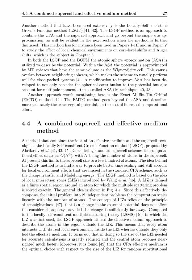
4.4 A combined supercell and effective mediummethod
A method that combines the idea of an effective medium and the supercell tech-nique is the Locally Self-consistent Green’s Function method (LSGF), proposed byAbrikosov et al. [41, 42, 45]. Considering standard supercell schemes the computa-tional effort scales as O(N3), with N being the number of atoms in the supercell.At present this limits the supercell size to a few hundred of atoms. The idea behindthe LSGF method is to find a way to provide better time scaling and still accountfor local environment effects that are missed in the standard CPA scheme, such asthe charge transfer and Madelung energy. The LSGF method is based on the ideaof local interaction zones (LIZs) introduced by Wang et al. [46]. A LIZ is definedas a finite spatial region around an atom for which the multiple scattering problemis solved exactly. The general idea is shown in Fig. 4.4. Since this effectively de-composes the initial problem into N independent problems the computation scaleslinearly with the number of atoms. The concept of LIZs relies on the principleof nearsightedness [47], that is a change in the external potential does not affectthe considered property provided the change is sufficiently far away. Comparedto the locally self-consistent multiple scattering theory (LSMS) [46], in which theLIZ was first used, the LSGF approach utilizes the effective medium approach todescribe the atoms in the region outside the LIZ. This means that every atominteracts with its real local environment inside the LIZ whereas outside they onlyfeel the effective medium. It turns out that in doing so the size of the LIZ neededfor accurate calculations is greatly reduced and the central atom becomes near-sighted much faster. Moreover, it is found [42] that the CPA effective medium isthe optimal choice with respect to the size of the LIZ for random substitutional

28 Electronic structure of random alloys
!"!"!"!"
"!"!"!"!
"!"!"!"!
!!"!!!"!
!"!"!"!"
"!"!"!"!
"!"!"!"!
!!"!!!"!
(a)
!!!!!!!!
!!!!!!!!
!!!!!!!!
!!!!!!!!
!!!!!!!!
!!!!!!!!
!!!!!!!!
!!!!!!!!
(b)
!!!!!!!!
!!!!!!!!
!!!!!!!!
!!!!"!!!
!!!!"!!!
!!!!!!!!
!!!!!!!!
!!!!!!!!
#$ %&#%
$&
(c)
!!!!!!!!
!!!!!!!!
!!!!!!!!
!!!"""!!
!!!!"!!!
!!!"!"!!
!!!!!!!!
!!!!!!!!
(d)
Figure 4.4. Illustration of the idea behind the locally self-consistent Green’s functionmethod. (a) A supercell with periodic boundary conditions is in subfigure (b) replaced byan effective medium (represented by gray atoms). Subfigures (c) and (d) show differentsizes of the so-called local interaction zone embedded into the effective medium. See textfor further explanation.
alloys and has also been the method of choice in the present work.
The procedure for solving the electronic structure problem is schematicallyshown in Fig. 4.4. From a supercell with a given distribution of atoms the effectivemedium is created (represented by gray atoms). For each atom in the originalsupercell the LIZ is embedded into the effective medium. The size of the LIZcan be tuned to include only the central site, the nearest neighbors, the nextnearest neighbors and so fourth. For each atom the Dyson equation is used tosolve the scattering problem inside the LIZ. If one considers an atom at site Rand surround it by M − 1 neighbors, i.e. forming a LIZ of M atoms, the Green’sfunction for the LIZ embedded into the effective medium can be found by solvingthe corresponding multisite equation. The Green’s function at the central site R

4.4 A combined supercell and effective medium method 29
O(N3)Tim
e
Number of atoms (N)
O(M3N)
O(M3N)
Figure 4.5. Schematic comparison ofthe required computational effort be-tween conventional O(N3) methods andthe order-N LSGF method with two dif-ferent sizes of the LIZ, denoted M andM with M > M . For a LIZ of size Mthe (‖) area denotes the supercell sizesfor which conventional electronic struc-ture methods are more efficient thanLSGF. The (‖)+(=) area denotes thecorresponding supercell sizes when us-ing a LIZ of size M .
can be written as [41]
gRR = gRR +
M∑
R′=1
gRR′(mR′ −mR′)gR′R, (4.13)
where summation runs over the atoms constituting the LIZ. The coherent pathoperator and the coherent potential function are designated by g and m, respec-tively. In general, the full Green’s function matrix gRR′ is not exact, because ofthe use of an effective medium instead of real atoms. However, the site diagonalblock gRR, which is needed to calculate the charge density, will approach that ofthe real atom at site R provided a sufficiently large LIZ is used. In this sense it islocally self-consistent [42].
Using the LSGF method one can study physical properties of individual atomsin a system. For instance the site-projected density of states can be calculated fromthe knowledge of gRR. The density of states at atoms with different number ofnearest neighbors of opposite kind in the equiatomic fcc AgPd and CuPd randomalloys shown in Fig. 1.2 have been calculated using this method.
Finally we note that the computational effort for each LIZ scales as O(M3).Therefore, an increased LIZ results in an increased slope in the computationaltime versus the number of atoms relation, but the overall linear behavior is stillmaintained, that is the complete procedure scales as O(M3N). This is illustratedin Fig. 4.5 where the computational time versus the number of atoms in the su-percell is schematically drawn for the case of the conventional supercell technique,O(N3), and when using the LSGF method, O(M3N). Two different sizes of theLIZ are chosen to simulate, for instance, the inclusion of the nearest neighbors andnext nearest neighbors in each LIZ. The different sizes of the LIZ are denoted Mand M respectively, assuming M being larger than M . Note that for moderatesupercells, or if a large LIZ is required, conventional O(N3) methods are moreefficient, as indicated by the marked areas in the figure.
A shortcoming with the present implementation of LSGF is the inability totreat local lattice relaxations.

30 Electronic structure of random alloys
4.5 Inhomogeneous lattice distortions
A consequence of different chemical environments is that the atoms that form thecrystal do not occupy ideal lattice positions. Instead, the atoms relax and arrangethemselves in a manner to minimize the total energy of the system. Inhomogeneouslattice distortions, or local lattice relaxations, are in general more pronounced foralloys where the constituents atoms have large size mismatches, such as CuAu [48,49].
Given the atomic distribution it is possible to calculate the forces acting on eachion by using the so-called force theorem or Hellmann-Feynman theorem [50, 51].The theorem states that the force acting on an ion is the same as the expectationvalue of the derivative of the Hamiltonian with respect to that ion position, thatis
Fi = − ∂E
∂Ri= −〈Ψ| ∂H
∂Ri|Ψ〉, (4.14)
where Ri is the position of the i:th ion and Ψ is an eigenfunction to H withH|Ψ〉 = E|Ψ〉. Actually, the theorem is more general and valid for variationof any parameter, not only the special case of nucleus positions as above. Thegeneralized form that applies to any variation λ is expressed as [4]
∂E
∂λ= 〈Ψλ|
∂H
∂λ|Ψλ〉. (4.15)
Using the equations above it is possible to show that the force can be written as
Fi = −∫n(r)
∂Vext(r)
∂Ridr − ∂Eion-ion
∂Ri, (4.16)
where Vext and Eion-ion denote the external potential and the interaction amongthe nuclei. Thus, the forces can be calculated from the knowledge of the electrondensity.
The force theorem gives a route to find the equilibrium positions of the nuclei.This can computationally be achieved in an iterative manner. Given the forcesacting on the ions the atoms can be moved a small step in the correspondingdirection. For this new arrangement of atoms we can find a new solution to theelectronic structure problem and recalculate new forces. This procedure is iterateduntil the forces are below some convergence criteria. Moreover, the theorem is alsoof use as a starting point for calculations of phonon spectra, see Section 7.2.2 ande.g. Ref. [52] for a thorough review.

CHAPTER 5
Disorder broadening of core levels:a local environment effect
Up to now I have outlined the general theory that has been used in the studies. Theforthcoming chapters are devoted to results. In each of the chapters I will overviewthe theoretical tools that were used to study the specific physical properties.
5.1 Introduction
Binding energies of core electrons in an atom can be measured experimentally, of-ten done using x-ray photoelectron spectroscopy (XPS). In the XPS technique thebinding energy spectra are obtained by irradiating the sample with a monochro-matic beam of photons, while simultaneously measuring the kinetic energy of theejected electrons, the so-called photoelectrons [53]. That is, if the incident photonhas sufficient energy, the binding energy Eb for an electron can be deduced fromthe knowledge of its kinetic energy Ekin and the photon energy ~ω
Eb = ~ω − Ekin. (5.1)
Above, the binding energy is assumed to be measured with respect to the Fermienergy as is common practice for solids [54]. By tuning the photon energy it ispossible to access different core-levels. Figure 5.1 shows a schematic of the XPSprocess together with the notation of electronic core-levels. Nowadays the XPStechnique is well established and routinely used to study a broad spectrum ofsystems such as metals, metallic alloys, semiconductors, polymers, ceramics etc.Further details of experimental techniques can be found in the book by Hufner [54]and references therein.
The binding energy of an electron is in general different depending on if weconsider e.g. the free atom, the atom placed in a crystal, for instance, a pure
31
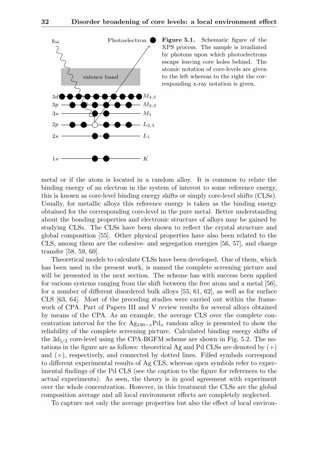
32 Disorder broadening of core levels: a local environment effect
1s K
2s L1
2p L2,3
3s M1
3p M2,3
3d M4,5
valence band
hω Photoelectron Figure 5.1. Schematic figure of theXPS process. The sample is irradiatedby photons upon which photoelectronsescape leaving core holes behind. Theatomic notation of core-levels are givento the left whereas to the right the cor-responding x-ray notation is given.
metal or if the atom is located in a random alloy. It is common to relate thebinding energy of an electron in the system of interest to some reference energy,this is known as core-level binding energy shifts or simply core-level shifts (CLSs).Usually, for metallic alloys this reference energy is taken as the binding energyobtained for the corresponding core-level in the pure metal. Better understandingabout the bonding properties and electronic structure of alloys may be gained bystudying CLSs. The CLSs have been shown to reflect the crystal structure andglobal composition [55]. Other physical properties have also been related to theCLS, among them are the cohesive- and segregation energies [56, 57], and chargetransfer [58, 59, 60].
Theoretical models to calculate CLSs have been developed. One of them, whichhas been used in the present work, is named the complete screening picture andwill be presented in the next section. The scheme has with success been appliedfor various systems ranging from the shift between the free atom and a metal [56],for a number of different disordered bulk alloys [55, 61, 62], as well as for surfaceCLS [63, 64]. Most of the preceding studies were carried out within the frame-work of CPA. Part of Papers III and V review results for several alloys obtainedby means of the CPA. As an example, the average CLS over the complete con-centration interval for the fcc Ag100−xPdx random alloy is presented to show thereliability of the complete screening picture. Calculated binding energy shifts ofthe 3d5/2 core-level using the CPA-BGFM scheme are shown in Fig. 5.2. The no-tations in the figure are as follows: theoretical Ag and Pd CLSs are denoted by (+)and (×), respectively, and connected by dotted lines. Filled symbols correspondto different experimental results of Ag CLS, whereas open symbols refer to exper-imental findings of the Pd CLS (see the caption to the figure for references to theactual experiments). As seen, the theory is in good agreement with experimentover the whole concentration. However, in this treatment the CLSs are the globalcomposition average and all local environment effects are completely neglected.
To capture not only the average properties but also the effect of local environ-

5.1 Introduction 33
0 20 40 60 80 100atomic % Pd
-1.2
-1.0
-0.8
-0.6
-0.4
-0.2
0
0.2
0.4
0.6
0.8C
ore-
leve
l shi
ft (e
V)
Figure 5.2. Calculated Ag 3d5/2 (+)and Pd 3d5/2 (×) core-level shifts usingthe CPA-BGFM framework as a functionof Pd concentration in the Ag100−xPdx
random alloy. Filled (open) symbols re-fer to different experimental results of theAg (Pd) CLSs. Squares are results fromRef. [65], circles from Ref. [66], and dia-monds are results collected from Ref. [67].
ments present in disordered alloys one needs to go beyond the single-site approxi-mation. It should be emphasized that even though it is rather simple to measurethe binding energies using XPS, it requires extremely high resolution spectrome-ters to explore the so-called disorder broadening of the photoemission spectra andhence to provide insight into the local chemical environments. As mentioned thedisorder broadening phenomenon arises due to the different local environmentsof the atoms in the alloy. Experimentally the core-spectral line attain a largerwidth as compared to the pure metal. Even though the effect has been overlookedfor quite some time, Cole et al. recently found the first experimental evidencefor disorder broadening of the 2p3/2 core spectral line of Cu in CuPd alloys [59].Later disorder broadenings have been detected in a number of binary alloys, forinstance the 3d5/2 core-level of Ag in AgPd [65], the 2p3/2 core-level in the Cubased alloys of Pd [68], Pt [69], Zn [70], and recently also the equiatomic CuAuwas examined [49].
Two examples of experimental core-level photoelectron spectra showing thedisorder broadening phenomenon are given in Fig. 5.3. The spectra show theadditional broadening effect present in the alloy compared to the pure metal. Thelargest disorder broadening measured so far, at least to my knowledge, is foundfor the 3d5/2 core level of Ag in the equiatomic AgPd random alloy. The spectrumis presented in the top panel of Fig. 5.3. On the contrary, one of the smallestbroadening observed is obtained for the 4f7/2 core level of Au in CuAu randomalloy, shown in the lower panel of Fig. 5.3. The data is collected from a reviewpaper [71] with results originally presented in Refs. [49, 65]. Note that the spectrahave been shifted in order to align the peaks. The identification of the effectof disorder broadening in alloys is interesting and opens up an opportunity forstudying specific local environments experimentally.
Soon after the experimental discovery, a theoretical work was carried out byFaulkner and co-workers [72]. They used the LSMS method, see Section 4.4 and

34 Disorder broadening of core levels: a local environment effect
1117 1117.5 1118 1118.5 1119Kinetic energy (eV)
0
20
40
60
80
100Co
unt r
ate
(arb
. uni
ts)
1402 1402.5 1403 1403.5 1404Kinetic energy (eV)
0
20
40
60
80
100
Coun
t rat
e (a
rb. u
nits)
Ag 3d5/2
Au 4f7/2
Figure 5.3. Experimental XPS spectrashowing the disorder broadening effect ofAg 3d5/2 core level in Ag50Pd50 (top panel)and the Au 4f7/2 core level in Cu50Au50
(bottom panel). Dashed lines and solidlines correspond to data obtained for thecase of the alloy and pure metal, respec-tively. The energy scales of the alloy spec-tra have been shifted by the same amountas the measured CLS in order to align thepeaks. The data is collected from Ref. [71].
Ref. [46], to account for the chemically different environments of the atoms. How-ever, the CLSs were calculated using an approximated scheme based on the Kohn-Sham energy-eigenvalues, the so-called initial state model which will be coveredlater, and rather poor agreement with experiment was found.
In this work I have calculated the disorder broadening of core spectral lines forseveral equiatomic random alloys employing the complete screening picture andsupercell methods. Before illuminating some of the results presented in Papers I–V, the theoretical tools to calculate CLSs are presented.

5.2 Modelling core-level shifts in disordered alloys 35
5.2 Modelling core-level shifts in disorderedalloys
5.2.1 Complete screening picture
Several different methods have been developed to analyze CLSs. Within the so-called potential model [58], the binding energy shift is estimated as
∆Epot = ∆V −∆R, (5.2)
where ∆V represents the shift of the electrostatic potential for an atom in differentenvironments and ∆R denotes the relaxation energy shift. The first term is referredto as the initial state shift, while the latter term accounts for the so-called finalstate effects, that is the relaxation effects due to the presence of a core-hole,see Fig. 5.1. The remaining electrons collectively screen the core hole and thisscreening combined with the core hole is felt by the escaping electron.
A model that accounts for both initial as well as final state effects is the com-plete screening picture introduced by Johansson et al. [56]. The method is a totalenergy approach and does not make any distinction between the two contribu-tions. It relies on the main assumption that the valence electrons attain a fullyrelaxed configuration in the presence of a core hole. This is expected to be validfor metallic systems due to the mobility of the electrons.
Within the complete screening picture the ionization energy is calculated bythe total energy difference between the unperturbed state and the state with a corehole at single core-ionized atoms. The ionization energy is given by the so-calledgeneralized thermodynamic chemical potential (GTCP) [73]
µi =∂E
∂c
∣∣∣∣c→0
, (5.3)
where c defines the concentration of core-ionized atoms in a system with totalenergy E. The subscript i denotes the particular core-level that is of interest, itcould for instance be the 2p level as in the illustration of the XPS event in Fig. 5.1.The complete screening CLS, ∆Ecs, is then given by taken the difference betweenthe GTCPs when the atom is situated in the alloy and when it is placed in thereference system, that is
∆Ecsi = µalloy
i − µrefi = ∆µi. (5.4)
In the particular studies of disorder broadening in random metallic alloys thereference system is taken to be the corresponding pure metal.
Core-ionized atoms are in actual calculations simulated by promoting an elec-tron from the core-level of interest to the valence band. In this way the overallcharge neutrality is maintained. That is, in practice the GTCP is derived fromthe ground state energies of the ionized state (constrained to have a core hole atlevel i) and the unperturbed state, yielding the following expression
µi =Eioni − E
∆c. (5.5)

36 Disorder broadening of core levels: a local environment effect
To study the disorder broadening of CLSs the supercell framework has beenemployed. In this case we have as many different GTCPs as the number of atomscontained in the supercell. If we consider a binary alloy AB, the alloy GTCP forcore-level i of the A atom at position I in the supercell may be derived as
µAIi =
EAion
Ii − E1/N
, (5.6)
where N correspond to the total number of sites in the supercell. The dispersion ofCLSs may then be studied by constructing a large SQS and calculate the bindingenergy shift for each atom. A measure of the deviation from the mean is given bythe Gaussian full width at half maximum (FWHM)
Γ = 2σ√
2 ln 2, (5.7)
where σ is the standard deviation of the distribution. At the equiatomic composi-tion a Gaussian broadening of the core XPS spectrum is expected [59, 65, 68, 69,70]. From the knowledge about the site specific CLS, the average CLS is readilycalculated.
If electronic structure codes with no explicit access to particular core-levels areused, e.g. methods based on pseudopotentials or the PAW technique, the CLScan still be calculated using the so-called equivalent core approximation. Thiswas actually the method that was first employed in conjunction with the completescreening picture [56]. Within this model the core hole problem is circumventedby approximating the core-ionized atom by its neighboring element in the periodictable. This is the reason for also being named the (Z + 1)-approximation. It isassumed that when the photoelectron has escaped from the sample the remainingelectrons effectively see a core with one extra proton which is nearly identical tothe core of the (Z + 1)-element. [74].
There is another method accounting for both initial state and final state effects,the so-called Slater-Janak transition state model [75, 76]. The validity of thismodel and its ability to calculate CLSs in metallic alloys has been studied and canbe found in Refs. [62, 77, 78]. Further description of the model is also found inthe suggested references above.
5.2.2 Initial state approximation
To gain further understanding about the CLSs it is useful to separate the shift incontributions arising from initial state and final state effects. The shift in the on-site electrostatic potential ∆V due to different environments of an atom is reflectedas rigid shifts in eigenenergies of deeply lying core-states. Therefore, the initialstate contribution to the shift is sometimes referred to as the core-level eigenvalueshift [74] and is for the A atom at position I in the alloy calculated as
∆Eisi = −εAI
i + εrefi . (5.8)
εIi and εrefi denote the Kohn-Sham eigenvalues of electronic core-level i in the alloy
and in the pure metal (the reference system), respectively. The eigenvalues areassumed to be aligned to the Fermi-level.

5.3 Disorder broadening of core photoemission spectra 37
Naturally, since the final state effects are completely ignored, the reliability ofthe initial state shift depends strongly upon the system of study. If one expectsthat the contribution from final state effects is negligible, or assumed to be can-celled between the studied system and the reference system, then the initial statemodel would serve as a good approximation. However, if the screening characterof the valence electrons in the alloy as compared to the pure metal differs, theimportance of relaxation effects increases [55, 79]. Moreover, if we recap to Sec-tion 2.3 where the Kohn-Sham eigenvalues were introduced we remember that theyhave, in principle, no other physical interpretation apart from yielding the correctground state charge density. Nevertheless, together with the complete screeningpicture the initial state shift may be used to estimate, simply by subtracting itscontribution, the part arising from final state effects.
The complete screening picture and the initial state approximation have beenused together with the LSGF approach to study the disorder broadening of corespectral lines. The equivalent core approximation has been applied in conjunctionwith the PAW technique, as implemented in vasp, to study the effect of locallattice relaxations. Those methods were outlined in Chapter 4. In some cases theCPA method as implemented in BGFM has been used for comparison of generaltrends and to global composition averages.
5.3 Disorder broadening of core photoemissionspectra
In Fig. 5.2 I showed the possibility to calculate average core-level binding energyshifts over the whole composition range using the complete screening picture.In this work, as outlined above, we generalized the model to simulate disorderbroadening of core photoemission spectra. The theoretical scheme was tested ontwo chosen model systems, the equiatomic fcc AgPd and CuPd random alloys. Thedisordered alloys were modelled by a large supercell (256 atoms) constructing usingthe SQS technique described in Section 4.2. Moreover, the electronic structure wassolved using the LSGF method with a LIZ that included the nearest as well asnext nearest atoms around the central site, see Section 4.4. For further details ofthe calculations I refer to Paper I.
The core-levels under investigation were the 3d5/2 of Ag and Pd and the 2p3/2
of Cu. A summary of the results is given in Table 5.1 where also a comparisonto experiment as well as to the previous study by Faulkner et al. [72] is done. Asseen from the table the disorder broadening, calculated according to Eq. (5.7), ofthe 3d5/2 level of Ag and 2p3/2 core-level of Cu are substantially larger than for3d5/2 core-level of Pd. Moreover, the theoretical prediction of the Ag disorderbroadening is in excellent agreement with the experimental finding. The completescreening picture predicts a FWHM parameter Γ to be 0.35 eV as compared to theexperimental value of 0.38 eV. Actually, if only the initial state effect is considereda disorder broadening of 0.27 eV is obtained, which is in agreement with theprevious study by Faulkner et al. (0.31 eV) who employed this model to calculatethe CLSs. Hence, if one accounts for the relaxation energy, due to the presence of

38 Disorder broadening of core levels: a local environment effect
Table 5.1. Experimental and calculated FWHM parameter Γ. Experimental results forthe disorder broadening of Ag 3d5/2 core spectral line is taken from Ref. [65] and thedata for the 2p3/2 level of Cu is from Refs. [59, 68]. Γcs denote the results of the disorderbroadening obtained in this work. The last column contains results obtained by meansof the LSMS method using the initial state scheme to derive the CLSs, see Ref. [72]. Allvalues are given in eV.
Alloy (core level) Γexp Γcs ΓisLSMS
AgPd (Ag 3d5/2) 0.38 0.35 0.31AgPd (Pd 3d5/2) 0.13 0.08
CuPd (Cu 2p3/2) 0.23 0.16 0.05CuPd (Pd 3d5/2) 0.06 0.10
the core hole, theoretical predictions are brought closer to experiment. This effectis also seen for the disorder broadening of the 2p3/2 core level of Cu, as seen inTable 5.1.
Unfortunately, in the case of Pd, a similar comparison between theory and ex-periment can not be done. Experimentally the identification of disorder broadeningis hindered by a large asymmetry in the XPS spectra. This effect has been at-tributed to low energy many-body excitations that varies with the local density ofstates at the Fermi-level and therefore also with local and global composition. [80]
A detailed investigation of the contributions arising from initial state as wellas final state effects was also carried out in Paper I. In Fig. 5.4 the broadeningsof the initial- and final state contributions are presented together with the totaldisorder broadening for the two alloys. Here the final state contribution to the CLSwas calculated as ∆Efs
i = ∆Ecsi − ∆Eis
i . The first observation is that the maincontribution to the CLSs of Ag and Cu arises from the initial state effect. Anotherobservation common to both Ag and Cu is that values around the maximum orminimum of the initial state and final state distributions were found to occur at thesame side of their respective average. In the figure this is illustrated by the dashedline that connects the end points of the distributions. This coupling between thedistributions effectively increases the total broadening. That is, for Ag and Cu,the effect of accounting for the core hole relaxation energy additionally increasesthe overall disorder broadening.
On the contrary, for Pd, the opposite effect is observed in both alloys. Thefinal state effect shift the average CLS in a profound way. Moreover, insteadof reinforcing the total broadening, the initial state and final state contributionscancel each other, with the result of a narrow total broadening. This is mostnotable in CuPd.
From this it is apparent that final state effects have a considerably impactand need to be considered in order to correctly predict disorder broadenings. Aninteresting note is that this effect actually correlates with the trend found for thevariation of the CLS as a function of the global concentration in CPA calculations.That is, the final state contribution is less pronounced at high Pd concentration.

5.3 Disorder broadening of core photoemission spectra 39
!!"# !!"$ !!"% !!"& !"!
(a) Ag 3d5/2
(b) Pd 3d5/2
'()*+!,-!"./,01
234)4*+!4,-!"&5,01
643*+!7,-!"!8,01
'()*+!,-!"9.,01
234)4*+!4,-!"9.,01
643*+!7,-!"&&,01
":;,<01=
!!"$ !!"& !"& !"$
Ag 3d5/2 Pd 3d5/2
!E (eV)
Initial!is = 0.27 eV
Total!cs = 0.35 eV
Total!cs = 0.13 eV
Final!fs = 0.09 eV
Final!fs = 0.22 eV
Initial!is = 0.13 eV
(a) Ag50Pd50
!!"# !!"$ !!"% !"!
&'()*
!+,!"-$+./
012(2)*!2+,!"--+./
321)*
!4+,!"!#+./
&'()*
!+,!"!$+./
012(2)*!2+,!"-5+./
321)*
!4+,!"-6+./
(a) Cu 2p3/2
(b) Pd 3d5/2
"78+9./:
!!"- !"- !"% !"6 !";
Cu 2p3/2
!E (eV)
Initial!is = 0.11 eV
Initial!is = 0.14 eV
Final!fs = 0.09 eV
Final!fs = 0.15 eV
Total!cs = 0.16 eV
Total!cs = 0.06 eV
Pd 3d5/2
(b) Cu50Pd50
Figure 5.4. Calculated disorder broadening according to the complete screening pic-ture and its separation into initial state (is) and final state (fs) contributions in the (a)Ag50Pd50 and (b) Cu50Pd50 random alloys. The final state contribution is defined as∆Efs
i = ∆Ecsi − ∆Eis
i .

40 Disorder broadening of core levels: a local environment effect
2 3 4 5 6 7 8 9 10No. of Pd atoms as nearest neighbors
-1.0
-0.8
-0.6
-0.4
-0.2
0
0.2C
LS (e
V)
Figure 5.5. The variation of the aver-age CLS as a function of the number ofPd atoms as nearest neighbors. Circlesand squares correspond to the average CLStaken over all sites with the same numberof Pd atoms as nearest neighbors for Pdand Ag, respectively.
This can be seen in either of the two included review Papers III (Fig. 5 on p. 131)or V (Fig. 5 on p. 154), with the original findings presented in Refs. [55, 62].Considering that the minimum of the final state distributions of Pd correspondsto environments with a high density of Pd atoms as nearest neighbors, this followsthe trend for the global composition variation. Moreover, in Fig. 5.5, the averageCLS as a function of the number of nearest neighbors of Pd atoms is shown.The average is taken over all sites with the same number of Pd atoms as nearestneighbors. The variation of the CLSs show similar dependency as found for theCLS as a function of the global composition presented in Fig. 5.2.
A last observation is that also the total average CLS, taken over all sites,agrees with experiment, taken into account that the experimental uncertaintyis the order of ±0.1 eV. Comparing experimental findings to the average CLS,given within parenthesis, we have for Ag in AgPd alloy that ∆Eexp
b = −0.62 eV(−0.49 eV) and for Pd ∆Eexp
b = −0.20 eV (−0.13 eV), for the case of CuPda similar comparison yields ∆Eexp
b = −0.64 eV (−0.77 eV) for Cu and for Pd∆Eexp
b = 0.19 eV (0.35 eV).
5.3.1 The influence of inhomogeneous lattice distortions
Even though it was shown that the contribution from the final state effect broughttheoretical predictions in closer agreement with experiment, it was considered if theneglect of inhomogeneous lattice distortions could have an impact on the disorderbroadening. Due to different local compositions around atoms, there will be locallattice relaxations that may influence the CLS.
The effect of local lattice relaxations was investigated in Paper I as a possibleexplanation to the somewhat worse agreement in the FWHM parameter Γ betweentheory and experiment for the case of Cu in CuPd. Subsequently, a joint experi-
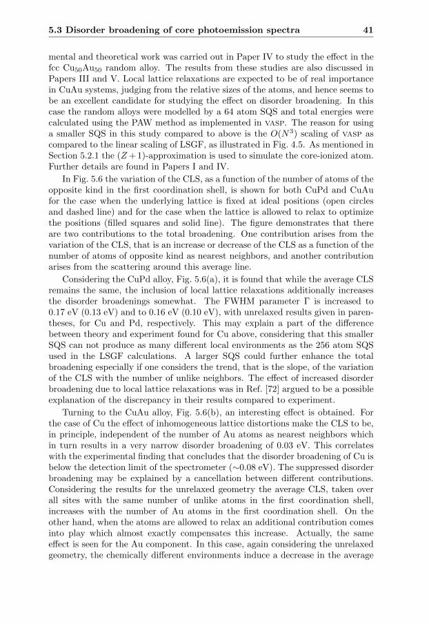
5.3 Disorder broadening of core photoemission spectra 41
mental and theoretical work was carried out in Paper IV to study the effect in thefcc Cu50Au50 random alloy. The results from these studies are also discussed inPapers III and V. Local lattice relaxations are expected to be of real importancein CuAu systems, judging from the relative sizes of the atoms, and hence seems tobe an excellent candidate for studying the effect on disorder broadening. In thiscase the random alloys were modelled by a 64 atom SQS and total energies werecalculated using the PAW method as implemented in vasp. The reason for usinga smaller SQS in this study compared to above is the O(N3) scaling of vasp ascompared to the linear scaling of LSGF, as illustrated in Fig. 4.5. As mentioned inSection 5.2.1 the (Z+ 1)-approximation is used to simulate the core-ionized atom.Further details are found in Papers I and IV.
In Fig. 5.6 the variation of the CLS, as a function of the number of atoms of theopposite kind in the first coordination shell, is shown for both CuPd and CuAufor the case when the underlying lattice is fixed at ideal positions (open circlesand dashed line) and for the case when the lattice is allowed to relax to optimizethe positions (filled squares and solid line). The figure demonstrates that thereare two contributions to the total broadening. One contribution arises from thevariation of the CLS, that is an increase or decrease of the CLS as a function of thenumber of atoms of opposite kind as nearest neighbors, and another contributionarises from the scattering around this average line.
Considering the CuPd alloy, Fig. 5.6(a), it is found that while the average CLSremains the same, the inclusion of local lattice relaxations additionally increasesthe disorder broadenings somewhat. The FWHM parameter Γ is increased to0.17 eV (0.13 eV) and to 0.16 eV (0.10 eV), with unrelaxed results given in paren-theses, for Cu and Pd, respectively. This may explain a part of the differencebetween theory and experiment found for Cu above, considering that this smallerSQS can not produce as many different local environments as the 256 atom SQSused in the LSGF calculations. A larger SQS could further enhance the totalbroadening especially if one considers the trend, that is the slope, of the variationof the CLS with the number of unlike neighbors. The effect of increased disorderbroadening due to local lattice relaxations was in Ref. [72] argued to be a possibleexplanation of the discrepancy in their results compared to experiment.
Turning to the CuAu alloy, Fig. 5.6(b), an interesting effect is obtained. Forthe case of Cu the effect of inhomogeneous lattice distortions make the CLS to be,in principle, independent of the number of Au atoms as nearest neighbors whichin turn results in a very narrow disorder broadening of 0.03 eV. This correlateswith the experimental finding that concludes that the disorder broadening of Cu isbelow the detection limit of the spectrometer (∼0.08 eV). The suppressed disorderbroadening may be explained by a cancellation between different contributions.Considering the results for the unrelaxed geometry the average CLS, taken overall sites with the same number of unlike atoms in the first coordination shell,increases with the number of Au atoms in the first coordination shell. On theother hand, when the atoms are allowed to relax an additional contribution comesinto play which almost exactly compensates this increase. Actually, the sameeffect is seen for the Au component. In this case, again considering the unrelaxedgeometry, the chemically different environments induce a decrease in the average

42 Disorder broadening of core levels: a local environment effect
3 4 5 6 7 8 9
-0.6
-0.4
-0.2
0
0.2
0.4
0.6
Cor
e-le
vel s
hift
(eV
)
3 4 5 6 7 8 9
-0.6
-0.4
-0.2
0
0.2
0.4
0.6C
ore-
leve
l shi
ft (e
V)
Cu
(b) CuAu(a) CuPd
Pd
Cu
Au
No. of atoms of opposite kind in the first coordination shell
Figure 5.6. Variation of the CLS as a function of the number of atoms of opposite kind inthe first coordination shell. The CLS of Cu 2p3/2 and Pd 3d5/2 is presented in (a) whereasin (b) the CLS of Cu 2p3/2 and Au 4f7/2 are shown. Open circles represent the site-resolved CLS for an unrelaxed underlying lattice. Filled squares are the correspondingCLS when accounting for local lattice relaxations. The lines represent the average CLStaken over all sites with equal amount of unlike nearest neighbors. The figure is takenfrom Paper V.
CLS as a function of Cu atoms in the first shell. However, here the effect ofinhomogeneous lattice distortions is so strong that the variation of the CLS withincreased number of Cu atoms as nearest neighbors is reversed. In the case ofAu the FWHM parameter is calculated to be 0.09 eV in good agreement withexperiment where an additional broadening of 0.12 eV is found for Cu50Au50 ascompared to pure Au. Another effect seen on Au but not on Cu is that the averageCLS changes when accounting for relaxations. In the case of Au the average CLSdecreases from 0.36 eV to 0.28 eV when the atoms are allowed to relax to optimalpositions, in close agreement with 0.25 eV as measured in experiments.
We conclude that for alloys with large size-mismatch between the components,the effect of local lattice relaxation can have a qualitative impact on the CLSs andthe disorder broadening of core-levels.
5.4 Disorder broadening of Auger spectra
Another experimental technique that is used to reveal information about the elec-tronic structure and bonding properties in solids is Auger electron spectroscopy(AES). As XPS, AES relies on the the fact that the kinetic energies of the ejectedelectrons are characteristics of the energy levels in the solid. In fact, the Augerprocess occurs after an electronic shell has been ionized, that is it can be seen as adecay route of the XPS event. In the XPS event a core-ionized atom is left behind.This hole may be filled by an electron that is less tightly bound. Simultaneouslythe excess of energy, i.e. the difference in orbital energies, may be captured by

5.4 Disorder broadening of Auger spectra 43
1s K
2s L1
2p L2,3
3s M1
3p M2,3
3d M4,5
valence band
hω Photoelectron
(a)
1s K
2s L1
2p L2,3
3s M1
3p M2,3
3d M4,5
valence band
Auger electron
(b)
Figure 5.7. Schematic view of the Auger process. (a) A core hole is created by irra-diating the sample. (b) As this corresponds to an unstable state an electron with lowerbinding energy can fill the vacancy. This excess of energy is captured by a third electron,the Auger electron, which escapes from the sample. The final state is an atom withdouble core holes. The atomic notation of core-levels is given to the left in each subfigurewhereas to the right the corresponding x-ray notation is given.
another outer shell electron that escapes from the sample, provided the energy islarge enough. The escaping electron is referred to as the Auger electron, in analogywith the photoelectron in the XPS process. The Auger process is schematicallydrawn in Fig. 5.7. It is common to use the x-ray notation when referring to Augerprocesses. The Auger electron in the example given in Fig. 5.7 would be referredto as an L2,3M2,3M4,5 electron. The first part, L2,3, labels the atomic level thatis filled in the process whereas the second part, M2,3, labels the atomic level fromwhere the relaxing electron leaves, and the last part, M4,5, represents the atomiclevel from which the Auger electron was emitted. The Auger kinetic energy canbe evaluated as
EAESkin (ijk) = Eb(i)− Eb(jk), (5.9)
where Eb(i) corresponds to the binding energy of an electron at i:th core-level andEb(jk) corresponds to the double core-hole binding energy at j and k. Hence, ijkrepresent the electronic shells that are involved in the process. Both the kinetic en-ergy of the photoelectron and the Auger electron can be measured simultaneously.This reduces the problem of the reference energy, since the difference in kineticenergy is obtained in the same spectra, and is thus independent of the referenceenergy of the spectrometer [81]. A parameter α that measures this difference wasintroduced by Wagner [82], later modified to α′ which also involves the photon

44 Disorder broadening of core levels: a local environment effect
energy of the excitation source, that is
α′ = α+ ~ω = EAESkin (ijk)− EXPS
kin (i) + ~ω= EAES
kin (ijk) + Eb(i). (5.10)
Here I have used Eq. (5.1) in the second equality to identify the binding energyEb(i). Extracting the Auger parameter enables to experimentally estimate theinitial state and final state contribution to the CLS [83, 71, 80, 84]
∆α′ = ∆EAESkin + ∆Eb ≈ 2∆R, (5.11)
∆EAESkin + 3∆Eb ≈ 2∆V. (5.12)
Theoretically it is straightforward to extend the complete screening pictureto also calculate the Auger kinetic energy shift as well as the shift of the Augerparameter [85]. This was done in Ref. [79] where the Auger shifts were analyzedas a function of the global composition, both experimentally as well as theoret-ically. Theoretically the Auger shifts were calculated using the CPA, effectivelyaveraging out the local environment effects. Excellent agreement between theoryand experiment was obtained. I will return to those results later when discussingthe disorder broadening of Auger spectra.
To study the disorder broadening effect the model is further extended. Givenrelation Eq. (5.9), the shift of the Auger kinetic energy between the alloy and apure metal can be calculated as
∆EAESkin (ijk) = ∆Eb(i)−∆Eb(jk)
= ∆µi −∆µjk, (5.13)
where the notation from Eq. (5.4) has been adopted. In a similar way, using therelation above, the Auger parameter shift may be calculated as
∆α′ = ∆EAESkin (ijk) + ∆Eb(i)
= 2∆µi −∆µjk. (5.14)
For transparency the site and occupation index AI has been suppressed. However,one should keep in mind that due to local environment effects, both EAES
kin (ijk) andα′ are site-specific quantities. In Paper V we studied the disorder broadening ofAuger L3M4,5M4,5 spectra in equiatomic random AgPd alloy. The same techniqueas above for the case of the AgPd alloy was used, that is we utilized the SQStechnique (256 atoms) and the electronic structure problem was solved using theLSGF method. In actual calculations the Auger process was simulated by a singlecore hole in 2p3/2 ↔ L3 and double core holes in 3d5/2 ↔ M4,5 (identical resultsare obtained if one instead considers two single holes in 3d3/2 and 3d5/2).
The simulated spectra of the Auger kinetic shifts and Auger parameter shiftsare shown in Fig. 5.8. Both components show similar disorder broadening of Augerkinetic energy shifts, 0.36 eV. That is, approximately the same FWHM parameteras for the 3d5/2 CLS is obtained in the case of Ag, but it is significantly increasedin the case of Pd, roughly by a factor of three.

5.4 Disorder broadening of Auger spectra 45
(a) Ag (b) Pd
-1.0 -0.8 -0.6 -0.4 -0.2 0 0.2 0.4 0.6 0.8 1.0Auger kinetic binding energy shifts (eV)
Coun
ts (a
rb. u
nits)
2 3 4 5 6 7 8 9 10No. of Pd atoms in the first shell
-0.2
0
0.2
0.4
0.6
0.8
ΔE ki
n (eV
)
20 40 60 80Conc. Pd (at. %) Γ=0.36 eV
-1.0 -0.8 -0.6 -0.4 -0.2 0 0.2 0.4 0.6 0.8 1.0Auger kinetic binding energy shifts (eV)
Coun
ts (a
rb. u
nits)
2 3 4 5 6 7 8 9 10No. of Pd atoms in the first shell
-0.8
-0.6
-0.4
-0.2
0
0.2
ΔE ki
n (eV
)
20 40 60 80Conc. Pd (at %)Γ=0.36 eV
-1.0 -0.8 -0.6 -0.4 -0.2 0 0.2 0.4 0.6 0.8 1.0Auger parameter shifts (eV)
Coun
ts (a
rb. u
nits)
2 3 4 5 6 7 8 9 10No. of Pd atoms in the first shell
-0.8
-0.6
-0.4
-0.2
0
0.2
Δα
´ (eV
)
Conc. Pd (at. %)20 40 60 80
Γ=0.03 eV
-1.0 -0.8 -0.6 -0.4 -0.2 0 0.2 0.4 0.6 0.8 1.0Auger parameter shifts (eV)
Coun
ts (a
rb. u
nits)
2 3 4 5 6 7 8 9 10No. of Pd atoms in the first shell
-0.8
-0.6
-0.4
-0.2
0
0.2
Δα
´ (eV
)
20 40 60 80Conc. Pd (at. %)Γ=0.26 eV
Figure 5.8. The distribution of L3M4,5M4,5 Auger kinetic energy shifts (top panels)and Auger parameter shifts (bottom panels) in equiatomic AgPd random alloy. Resultsfor Ag and Pd are presented in the left and right panels respectively. The inset shows thevariation of the quantity, averaged over sites with the same number of atoms of oppositekind as nearest neighbors, with increasing Pd atoms in the first coordination shell (filledcircles). Those results are compared to results obtained by means of CPA [79] (opencircles).
Turning to the distribution of the Auger parameter shifts, an extremely sharpand narrow peak around zero is obtained in the case of Ag while a substantialbroadening and a non-zero average is obtained for Pd. Since ∆α′ is connectedto the final state contribution, this correlates with the previous discussion of theimportance of final state effects in the case of Pd as compared to Ag.
If we make a similar comparison as before and study the variation of the distri-butions as a function of the number of nearest neighbors of Pd atoms in the firstcoordination shell, a remarkable resemblance to the global composition variation isfound. This is the case considering both the Auger kinetic energy shifts and Augerparameter shifts, as seen in the insets to each of the panels in Fig. 5.8. Filled circlesdenote the variation of the average quantity as a function of increasing number ofPd atoms as nearest neighbors, and open circles correspond to the dependency onthe global composition variation derived using CPA. Results obtained using theCPA method are from Paper III and originally presented in Ref. [79]. Again theaverage is taken over all sites with the same number of Pd atoms as nearest neigh-bors. It is interesting to see the correlation, because one should remember thatthe CPA medium outside the LIZ describes the equiatomic composition whereasin the single-site calculations the medium describes the average properties of the

46 Disorder broadening of core levels: a local environment effect
Table 5.2. Average Auger L3M4,5M4,5 data calculated using the LSGF method arecompared to results obtained by means of CPA [79] as well as to experimental results [79].Data for the equiatomic alloy are presented and all values are given in eV.
∆EAESkin ∆α′
Ag LSGF 0.42 -0.06CPA 0.41 -0.11Exp. 0.41 -0.21
Pd LSGF -0.32 -0.44CPA -0.32 -0.41Exp. -0.38 -0.59
corresponding global composition. In Table 5.2 the results for the equiatomic com-position of the Auger shifts are compiled and compared to experiment as well asto results obtained by means of CPA.
Recently, Stoker et al. [80] have pointed out that a comparison of disorderbroadening in the XPS and Auger spectra should allow for experimental separa-tion of initial and final state broadenings. Also, the prospects of measuring thedisorder broadening of the Auger spectra was investigated. They parameterizedthe initial state and final state distributions presented in Fig. 5.4 and deducedthe Auger disorder broadening to be greater than the XPS disorder broadeningand to be in the order of 0.3–0.5 eV [71, 80], in line with the results presentedabove, derived from first-principles. On the other hand they also observed, usingthe parameterization, that it will be hard to measure the Auger disorder broaden-ing in Ag50Pd50 and Cu50Pd50 alloys. Nevertheless, they identified a number ofother Auger transitions in other systems for which the disorder broadening may bedetectable experimentally. It would be interesting to calculate the disorder broad-ening of Auger shifts in these systems for possible comparison to experiments.
CHAPTER 6
Local environment effects in magnetic FeNi alloy
6.1 Introduction
In Paper VI the effect of local environments on the electronic structure and physicalproperties of magnetic systems was considered. Magnetism gives a system anadditional degree of freedom in the sense that the system can lower its energy byattaining different magnetic orderings. Among others, common magnetic states areferromagnetic, antiferromagnetic, spin-waves, and states where the moments arealigned in a disordered manner. Ferromagnetic and antiferromagnetic orderingsare states where the moments align collinearly, whereas the latter two are so-callednon-collinear states.
Here the collinear order was treated and as a model system the random equi-atomic fcc FeNi alloy was studied. Fe–Ni steels are interesting alloys because ofthe so-called Invar effect that at ambient conditions appears at around 35 atomicpercent Ni. The Invar effect is characterized by a very low thermal expansion coef-ficient over a wide temperature range. The anomalous behavior was recognized byGuillaume already in 1897 [86]. Invar alloys are used in a wide variety of applica-tions. Obviously they are particularly useful when high dimensional stability withrespect to variation in temperature is required, like for instance in precision instru-ments where minimum thermal expansion is vital. The effect was later observedin other iron-based alloys, for instance Fe-Pd and Fe-Pt.
The Invar effect has attracted much attention and efforts have been made intrying to understand the physical origin behind the vanishing expansion. Weiss [87]proposed a two-state model upon which the Fe atoms can attain two states: onehigh-spin state, ferromagnetic, with large volume, and another low spin-state, an-tiferromagnetic, with smaller volume. Thermal excitations into the low-spin statewas an explanation of the low expansion coefficient. More recent non-collinear cal-
47

48 Local environment effects in magnetic FeNi alloy
culations by Schilfgaarde et al. [88] predict that the situation is far more complex.According to their calculations at 0 K the Fe65Ni35 alloy is ferromagnetic whileupon compression a few Fe spins make discontinuous transitions to approximatelyantiferromagnetic alignment. Upon further reduction of the volume a continuoustransition to a disordered non-collinear state is observed. The appearance of theInvar effect was suggested to be an effect of a large amount of magnetic configu-rations within a certain volume range. That is, upon external perturbations thesystem can relax into another magnetic configuration instead of expanding thelattice. Moreover, it was suggested that the Invar anomaly may be induced uponcompression of the lattice in non-Invar alloys. This was later confirmed experi-mentally in Fe55Ni45 and Fe20Ni80 alloys [89]. Ruban et al. [90] studied the originof the magnetic frustration in the region of the Invar effect and concluded thatit was caused by the local environment effects. Although the models have pro-vided insight into the mechanism, a full explanation of the effect is still lacking.Nevertheless, progress in the field is ongoing, see e.g. Refs. [91, 92, 93, 94, 95, 96].
The aim with our study was not to find a general explanation for the Invareffect, rather the system was chosen to study the importance of local environmenteffects, especially in the vicinity of magnetic instabilities.
6.2 The influence of local chemical environments
In the simulations we approach the magnetic instability from the high volumeferromagnetic side. Moreover, the only allowed deviations from collinear ferro-magnetic state are possible spin-flips. Using the SQS approach together with theGreen’s function technique, the magnetic moments and pair exchange interactionswere studied at different volumes and at sites with different local chemical envi-ronments.
In the absence of external fields and if only pair interactions are considered,the classical Heisenberg Hamiltonian that describes the exchange interactions maybe written as
Hex = −∑
i6=j
Jijei · ej , (6.1)
where ei is an unit vector pointing in the same direction as the magnetic momentat site i. The summation runs over all pairs excluding i = j. Jij are the pairexchange parameters that may be obtained using the Green’s function techniquethrough the magnetic force theorem [97, 98, 99]. For a ferromagnetic referencesystem the pair exchange interactions can be calculated as
Jij =1
4π
EF∫Im Tr(∆ig
↑ij∆jg
↓ji)dE, (6.2)
where ∆i = m↑i − m↓i is the difference in the potential functions and gij is thescattering path operator, see Section 3.4. Positive Jij favors ferromagnetic orderingwhereas negative interactions indicate a tendency towards antiferromagnetism. Inthe Hamiltonian the moments are treated as classical vectors and it is assumed

6.2 The influence of local chemical environments 49
exchange parameter of the classical Heisenberg Hamilto-nian Hex ! "
P0ij Jijeiej. Here Jij are the pair exchange
parameters, ei is the unit vector in the direction of themagnetic moment of an atom at site i, and the summationruns over all sites i; j, excluding i ! j. The effectiveexchange parameter J0 !
Pja0 J0j can be calculated
independently of Jij using the magnetic force theorem[17–19]. The physical meaning of J0 is the following: itmeasures the energy cost for the rotation of one spin at site0 by the small angle y from the original orientation in asystem with, for example, the ferromagnetic long-rangeorder. Therefore, negative sign of J0 indicates a tendencytowards a spin flip transition at a given site. In Fig. 2 weshow local magnetic moments and effective exchangeparameters at different sites of fcc Fe50Ni50 alloy as afunction of the lattice parameter. The alloy is simulated by64 atom SQS [15,16]. One can clearly see that the valuesexhibit a substantial dispersion. In agreement with theresults reported earlier in Ref. [23], we see in Fig. 2a thatthe amplitude of magnetic moments at different Fe sites
anticorrelates with number of Fe atoms in the firstcoordination shell of the sites. Moreover, we observe thatat lattice parameter 3.45 A magnetic moments at some Fesites discontinuously flip, and orient antifrerromagneticallyto the rest of Fe moments in the supercell. Similartransition was observed by van Schilfgaarde et al. [4] innon-collinear calculations for Fe65Ni35 Invar alloy. Thetransition for equiatomic alloy occurs at a smaller volume,though, in agreement with the fact that the Invar effect inalloys with higher Ni concentration can be induced bycompression [24]. Note that the sites where the spin-fliptransition takes place are in the Fe-rich environment.The behavior of magnetic moments agrees with the
behavior of effective exchange parameters shown inFig. 2b. J0 also show substantial variations depending onthe local chemical composition around their sites. Thedispersion increases with decreasing lattice parameter, andbecomes particularly strong in a vicinity of the first spin fliptransition. The effective exchange parameters at Fe sites inFe-rich environment are smaller than J0 at Fe sitessurrounded by more Ni atoms. The former change signfirst, indicating a tendency for the local moments at theirrespective sites to be aligned antiparallel to the direction ofnet magnetization. According to Ref. [4] these spin flipscatalyze the transition to a non-collinear alignment forsmaller lattice constants, and act as a nucleation centers forthe continuous transition from the HS ferromagnetic stateat large volumes to the LS non-collinear state at smallervolumes.In order to understand the observed behavior of effective
exchange parameters in fcc Fe–Ni Invar, let us consider theinfluence of the local chemical environment on theelectronic structure at different sites in the bulk alloys. InFig. 3 we show the DOS calculated for three Fe sites in thesupercell with 9, 6 and 3 Fe atoms in the first coordinationshell, respectively, and at two different lattice parameters.Let us first point out that differences between the DOS atdifferent Fe sites are quite small; they are definitely muchsmaller than, for instance, the difference between theelectronic structure of the bulk and thin film alloysdiscussed in Section 3.1. Still, it is responsible for thesubstantial dispersion of the effective exchange parametersin Fig. 2b. Upon the close inspection of Fig. 3 one sees thatthe most noticeable difference between the DOS atdifferent sites consists of the shift of the majority spin d-band towards the Fermi energy upon decreasing intera-tomic distance and increasing number of Fe atoms in thefirst coordination shell. The same tendency we saw than wediscussed a suppression of magnetic phase transition inthin films as compared to bulk Fe–Ni alloys. Indeed, inFig. 1a one sees that in the bulk alloys the majority spin d-band is not saturated, opposite to the thin film case. Wetherefore conclude that the tendency towards the anti-ferromagnetism correlates with the fact that the spin upstates becomes unsaturated upon compression of thelattice, and that the tendency is stronger in Fe-richenvironment.
ARTICLE IN PRESS
3.4 3.5 3.6 3.7Lattice parameter (Å)
-2
0
2
4
6
8
10
12
J 0 (m
Ry)
(a)
(b)
Fe (3Fe-9Ni)
Fe (4Fe-8Ni)
Fe (5Fe-7Ni)
Fe (6Fe-6Ni)
Fe (8Fe-4Ni)
Fe (9Fe-3Ni)
-1
0
1
2
m (m
B)
Fe (3Fe-9Ni)
Fe (8Fe-4Ni)
Fe (9Fe-3Ni)
Fig. 2. (a) Local magnetic moments m in Bohr magnetons #mB$ and (b)effective exchange parameters J0 at different sites of fcc Fe50Ni50 alloy as afunction of the lattice parameter. The alloy is simulated by 64 atom SQS[15,16]. Each site shown in the figure has different number of Fe and Ninearest neighbors, as indicated in the legends.
I.A. Abrikosov et al. / Journal of Magnetism and Magnetic Materials 300 (2006) 211–215214
Figure 6.1. (a) Local magnetic mo-ments m, in units of Bohr magnetonsmB, and (b) effective exchange inter-actions J0, in mRy, at different sitesas a function of the lattice parameterin the equiatomic fcc FeNi alloy. Grayshaded areas indicate negative valuesof the corresponding quantity. Thevolume for the first observed spin-fliptransition is indicated by the verticalline. The figure is taken from Pa-per VI.
that one can ascribe local magnetic moments to each site. In general the magneticdensity is a vector field, but often the so-called atomic moment approximation isused. This is motivated by noticing that the spin density often is concentratedand aligned in a collinear manner centered around the nuclei [100].
One may also define an effective exchange parameter J0:
J0 =∑
j 6=0
J0j (6.3)
This parameter describes the energy cost upon rotating a spin at site 0 a smallangle from the original alignment in a system with, for instance as treated here,ferromagnetic order. Moreover, if J0 < 0 this is an indication of a tendency towardsa spin-flip at site 0.
Local magnetic moments and effective exchange parameters at different sites asa function of the volume in the fcc Fe50Ni50 random alloy are shown in Fig. 6.1. Asseen, the local magnetic moments, Fig. 6.1(a), are sensitive to the local chemicalenvironment, in agreement with the results reported in Ref. [101] and what is foundin Paper II for a fixed volume. At large volumes the dependency is suppressedand almost identical local magnetic moments are observed, irrespective if the firstcoordination shell is mostly composed of Fe or Ni neighbors. While compressingthe lattice the local magnetic moment at a given site decreases almost linearly andthe spread in moments among different sites is increased with an anticorrelation

50 Local environment effects in magnetic FeNi alloy
4. Summary
In summary, we have shown that there exists asubstantial dependence of the site projected electronicstructure and magnetic properties in disordered systems onthe local chemical environment of the sites. The sites withmore Fe nearest neighbors exhibit stronger tendencytowards the antiferromagnetism. The tendency correlateswith the fact that the majority spin d-band is less saturatedin Fe-rich environment.
Acknowledgements
We are grateful to the Swedish Research Council (VR),EURTN project COLLECT, and The Swedish Foundation
for Strategic Research (SSF) for financial support. Thecollaboration between Sweden and the former SovietUnion was supported by The Royal Swedish Academy ofSciences. Dr. S.I. Simak is gratefully acknowledged forproviding us with the special quasirandom structureSQS-64.
References
[1] C.E. Guillaume, C. R. Acad. Sci. 125 (1897) 235.[2] E.F. Wasserman, in: K.H.J. Buschow, E.P. Wohlfarth (Eds.),
Ferromagnetic Materials, vol. 5, North-Holland, Amsterdam, 1990,p. 237 and references wherein.
[3] R.J. Weiss, Proc. R. Soc. London 82 (1963) 281.[4] M. van Schilfgaarde, I.A. Abrikosov, B. Johansson, Nature 400
(1999) 46.[5] A.K. Arzhnikov, L.V. Dobysheva, J. Magn. Magn. Mater. 117 (1992)
87.[6] W. Olovsson, I.A. Abrikosov, J. Appl. Phys. 97 (2005) 10A317.[7] A.V. Ruban, M.I. Katsnelson, W. Olovsson, S.I. Simak, I.A.
Abrikosov, Phys. Rev. B 71 (2005) 054402.[8] E.I. Kondorskii, V.L. Sedov, JETP 35 (1958) 1597.[9] V.L. Sedov, Antiferromagnetism of Gamma-iron. Problem of Invar,
Nauka, Moscow, 1987.[10] O.K. Andersen, Phys. Rev. B 12 (1975) 3060.[11] O.K. Andersen, O. Jepsen, Phys. Rev. Lett. 53 (1984) 2571.[12] P. Hohenberg, W. Kohn, Phys. Rev. B 136 (1964) 864.[13] W. Kohn, L.J. Sham, Phys. Rev. 140 (1965) A1133.[14] J.S. Faulkner, Prog. Mater. Sci. 27 (1982) 1.[15] A. Zunger, S.-H. Wei, L.G. Ferreira, J.E. Bernard, Phys. Rev. Lett.
65 (1990) 353.[16] A.V. Ruban, S.I. Simak, S. Shallcross, H.L. Skriver, Phys. Rev. B 67
(2003) 214302.[17] A.I. Liechtenstein, M.I. Katsnelson, V.A. Gubanov, J. Phys. F 14
(1984) L125.[18] A.I. Liechtenstein, M.I. Katsnelson, V.A. Gubanov, Solid State
Commun. 54 (1985) 327.[19] A.I. Liechtenstein, M.I. Katsnelson, V.P. Antropov, V.A. Gubanov,
J. Magn. Magn. Mater. 67 (1987) 65.[20] A.I. Abrikosov, H.L. Skriver, Phys. Rev. B 47 (1993) 16532.[21] A.V. Ruban, H.L. Skriver, Compt. Mat. Sci. 15 (1999) 119.[22] I.A. Abrikosov, O. Eriksson, P. Soderlind, H.L. Skriver, B.
Johansson, Phys. Rev. B 51 (1995) 1058.[23] P. James, O. Eriksson, B. Johansson, I.A. Abrikosov, Phys. Rev. B 59
(1999) 419.[24] L. Dubrovinsky, N. Dubrovinskaia, I.A. Abrikosov, M. Vennstrm,
F. Westman, S. Carlson, M. van Schilfgaarde, B. Jonansson, Phys.Rev. Lett. 86 (2001) 4851.
[25] F.O. Schuman, S.Z. Wu, G.J. Mankey, R.F. Willis, J. Appl. Phys. 79(1996) 5635.
[26] G.J. Mankey, S.Z. Wu, F.O. Schuman, F. Huang, M.T. Kief, R.F.Willis, J. Vac. Sci. Technol. A 13 (1995) 1531.
[27] E.A. Smirnova, I.A. Abrikosov, Yu.Kh. Vekilov, B. Johansson, A.N.Baranov, V.S. Stepanyuk, W. Hergert, P.H. Dederichs, Phys. Rev. B59 (1999) 14417.
ARTICLE IN PRESS
spin up
spin down
spin down
spin up
a=3.72 Å
a=3.49 Å
(9Fe-3Ni)
(6Fe-6Ni)
(3Fe-9Ni)
E-EF (Ry)0.2-0.2-0.4 0.0
20
10
0
10
20
20
10
0
10
20
DO
S (s
tate
s/ (R
y*at
om))
(a)
(b)
Fig. 3. Density of states (DOS) at different sites of fcc Fe50Ni50 alloy attwo different lattice parameters, corresponding to a high-spin ferromag-netic state (a) and a state in a vicinity of the first spin flip transition (b).Each site shown in the figure has different number of Fe and Ni nearestneighbors, as indicated in the legends.
I.A. Abrikosov et al. / Journal of Magnetism and Magnetic Materials 300 (2006) 211–215 215
(a)
(b)
DOS(states/(R
y·atom
))
E ! Ef (Ry)
4. Summary
In summary, we have shown that there exists asubstantial dependence of the site projected electronicstructure and magnetic properties in disordered systems onthe local chemical environment of the sites. The sites withmore Fe nearest neighbors exhibit stronger tendencytowards the antiferromagnetism. The tendency correlateswith the fact that the majority spin d-band is less saturatedin Fe-rich environment.
Acknowledgements
We are grateful to the Swedish Research Council (VR),EURTN project COLLECT, and The Swedish Foundation
for Strategic Research (SSF) for financial support. Thecollaboration between Sweden and the former SovietUnion was supported by The Royal Swedish Academy ofSciences. Dr. S.I. Simak is gratefully acknowledged forproviding us with the special quasirandom structureSQS-64.
References
[1] C.E. Guillaume, C. R. Acad. Sci. 125 (1897) 235.[2] E.F. Wasserman, in: K.H.J. Buschow, E.P. Wohlfarth (Eds.),
Ferromagnetic Materials, vol. 5, North-Holland, Amsterdam, 1990,p. 237 and references wherein.
[3] R.J. Weiss, Proc. R. Soc. London 82 (1963) 281.[4] M. van Schilfgaarde, I.A. Abrikosov, B. Johansson, Nature 400
(1999) 46.[5] A.K. Arzhnikov, L.V. Dobysheva, J. Magn. Magn. Mater. 117 (1992)
87.[6] W. Olovsson, I.A. Abrikosov, J. Appl. Phys. 97 (2005) 10A317.[7] A.V. Ruban, M.I. Katsnelson, W. Olovsson, S.I. Simak, I.A.
Abrikosov, Phys. Rev. B 71 (2005) 054402.[8] E.I. Kondorskii, V.L. Sedov, JETP 35 (1958) 1597.[9] V.L. Sedov, Antiferromagnetism of Gamma-iron. Problem of Invar,
Nauka, Moscow, 1987.[10] O.K. Andersen, Phys. Rev. B 12 (1975) 3060.[11] O.K. Andersen, O. Jepsen, Phys. Rev. Lett. 53 (1984) 2571.[12] P. Hohenberg, W. Kohn, Phys. Rev. B 136 (1964) 864.[13] W. Kohn, L.J. Sham, Phys. Rev. 140 (1965) A1133.[14] J.S. Faulkner, Prog. Mater. Sci. 27 (1982) 1.[15] A. Zunger, S.-H. Wei, L.G. Ferreira, J.E. Bernard, Phys. Rev. Lett.
65 (1990) 353.[16] A.V. Ruban, S.I. Simak, S. Shallcross, H.L. Skriver, Phys. Rev. B 67
(2003) 214302.[17] A.I. Liechtenstein, M.I. Katsnelson, V.A. Gubanov, J. Phys. F 14
(1984) L125.[18] A.I. Liechtenstein, M.I. Katsnelson, V.A. Gubanov, Solid State
Commun. 54 (1985) 327.[19] A.I. Liechtenstein, M.I. Katsnelson, V.P. Antropov, V.A. Gubanov,
J. Magn. Magn. Mater. 67 (1987) 65.[20] A.I. Abrikosov, H.L. Skriver, Phys. Rev. B 47 (1993) 16532.[21] A.V. Ruban, H.L. Skriver, Compt. Mat. Sci. 15 (1999) 119.[22] I.A. Abrikosov, O. Eriksson, P. Soderlind, H.L. Skriver, B.
Johansson, Phys. Rev. B 51 (1995) 1058.[23] P. James, O. Eriksson, B. Johansson, I.A. Abrikosov, Phys. Rev. B 59
(1999) 419.[24] L. Dubrovinsky, N. Dubrovinskaia, I.A. Abrikosov, M. Vennstrm,
F. Westman, S. Carlson, M. van Schilfgaarde, B. Jonansson, Phys.Rev. Lett. 86 (2001) 4851.
[25] F.O. Schuman, S.Z. Wu, G.J. Mankey, R.F. Willis, J. Appl. Phys. 79(1996) 5635.
[26] G.J. Mankey, S.Z. Wu, F.O. Schuman, F. Huang, M.T. Kief, R.F.Willis, J. Vac. Sci. Technol. A 13 (1995) 1531.
[27] E.A. Smirnova, I.A. Abrikosov, Yu.Kh. Vekilov, B. Johansson, A.N.Baranov, V.S. Stepanyuk, W. Hergert, P.H. Dederichs, Phys. Rev. B59 (1999) 14417.
ARTICLE IN PRESS
spin up
spin down
spin down
spin up
a=3.72 Å
a=3.49 Å
(9Fe-3Ni)
(6Fe-6Ni)
(3Fe-9Ni)
E-EF (Ry)0.2-0.2-0.4 0.0
20
10
0
10
20
20
10
0
10
20
DO
S (s
tate
s/ (R
y*at
om))
(a)
(b)
Fig. 3. Density of states (DOS) at different sites of fcc Fe50Ni50 alloy attwo different lattice parameters, corresponding to a high-spin ferromag-netic state (a) and a state in a vicinity of the first spin flip transition (b).Each site shown in the figure has different number of Fe and Ni nearestneighbors, as indicated in the legends.
I.A. Abrikosov et al. / Journal of Magnetism and Magnetic Materials 300 (2006) 211–215 215
Figure 6.2. Density of states at differ-ent Fe sites in the equiatomic fcc FeNialloy are calculated at (a) a high vol-ume, corresponding to a high-spin fer-romagnetic state, and at (b) a volume inthe vicinity of the first spin-flip transi-tion. The figure is taken from Paper VI.
between the amplitude and the number of Fe atoms as nearest neighbors. Uponfurther compression some Fe sites in Fe rich environments discontinuously flip toan antiferromagnetic alignment compared to the rest of the Fe atoms. This occurswhen the lattice parameter is close to 3.45 A, which is marked with a verticalline in the figure. At the Invar composition similar transitions occur at highervolumes [88], though the result is in agreement with the fact that the Invar effectmay be induced upon applying pressure.
A correlation to the results discussed above is seen in the effective exchangeinteractions, as shown in Fig. 6.1(b). Similar sensitivity to different chemical en-vironments is observed. Moreover, the variation of the exchange parameter as afunction of the lattice parameter is the same as for the local magnetic moments,i.e. while decreasing the volume the dispersion increases. At equilibrium latticeparameter, at around 3.55 A, all effective exchange parameters and local magneticmoments are positive, which is in agreement with the fact that Fe50Ni50 is fer-romagnetic at ambient pressure. Effective exchange interactions are smallest atFe sites with high concentration of its own kind as nearest neighbors. Close tothe lattice parameter 3.45 A, J0 changes sign at Fe sites in Fe rich environments,indicating a tendency towards spin-flip.
In Fig. 6.2 the density of states at three different Fe sites are shown at twodifferent volumes. Each site having different local chemical environments, that is 3,6 or 9 Fe atoms in the first coordination shell. The larger volume corresponds to ahigh-volume high-spin ferromagnetic state whereas the smaller volume corresponds

6.2 The influence of local chemical environments 51
to the lattice parameter in the vicinity of the first spin-flip transitions, see Fig. 6.1.Considering the site-projected density of states at the larger volume the spin up d-band is saturated at all sites, i.e. it is situated well below the Fermi level. However,upon compression of the lattice to a volume close to the one in the vicinity of spin-flip transitions, one notices that the spin up band is shifted towards the Fermi level.This is particularly pronounced for Fe atoms in Fe rich environments. Hence, thetendency towards antiferromagnetism correlates with the fact that the spin upstates become unsaturated.
Hence, there is strong dependence of the physical properties on the local chem-ical environment of the sites. Fe atoms in Fe rich environments exhibit strongertendency towards antiferromagnetism.

52 Local environment effects in magnetic FeNi alloy

CHAPTER 7
Local environment effects andthermodynamic stability in inhomogeneous systems
In the preceding chapters the local environment effects present in bulk alloys werehighlighted. The forthcoming chapter will focus on inhomogeneous systems. Inparticular, in Paper VII a joint theoretical and experimental study of structuralproperties of ultrathin AgPd films deposited on Ru was carried out. This will bediscussed in the next section. After that, I will discuss results from Paper VIIIwhere it was investigated if the presence of TiN interfaces modify the dynamicand thermodynamic stability of SiN.
7.1 Double-segregation effect in AgPd thin filmalloy
7.1.1 Introduction
Thin film alloys deposited on substrates are interesting because they often exhibitdifferent physics as compared to bulk. Some frequently used applications of thinfilms are electronics, catalysis and coatings of different kinds, e.g., wear-resistantcoatings on drills and optical coatings. The reduced dimensionality induces localenvironment effects that are not necessarily present in the bulk. Those effectsmay change the electronic structure significantly and give novel properties thatare highly desirable in applications. It is of importance to be able to determinethe variation of the composition through the thin film layers in order to predictthe physical properties.
Here we have studied a four-monolayer (ML) Ag1−xPdx thin film, with nominalequiatomic composition, deposited at a Ru(0001) substrate. The aim was to study
53
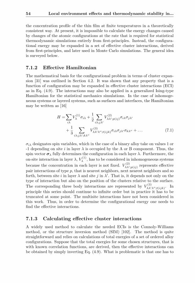
54 Local environment effects and thermodynamic stability in...
the concentration profile of the thin film at finite temperatures in a theoreticallyconsistent way. At present, it is impossible to calculate the energy changes causedby changes of the atomic configurations at the rate that is required for statisticalthermodynamic simulations entirely from first-principles. Instead, the configura-tional energy may be expanded in a set of effective cluster interactions, derivedfrom first-principles, and later used in Monte Carlo simulations. The general ideais surveyed below.
7.1.2 Effective Hamiltonian
The mathematical basis for the configurational problem in terms of cluster expan-sion [31] was outlined in Section 4.2. It was shown that any property that is afunction of configuration may be expanded in effective cluster interactions (ECI)as in Eq. (4.9). The interactions may also be applied in a generalized Ising-typeHamiltonian for the statistical mechanics simulations. In the case of inhomoge-neous systems or layered systems, such as surfaces and interfaces, the Hamiltonianmay be written as [16]
H =∑
iλ
V(1)λ σiλ +
1
2
∑
iλ;jλ′
V(2)λλ′;p(ij)σiλσjλ′
+1
3
∑
iλ;jλ′;kλ′′
V(3)λλ′λ′′;t(ijk)σiλσjλ′σkλ′′ + . . . (7.1)
σiλ designates spin variables, which in the case of a binary alloy take on values 1 or-1 depending on site i in layer λ is occupied by the A or B component. Thus, thespin vector σλ fully determines the configuration in each layer λ. Furthermore, the
on-site interaction in layer λ, V(1)λ , has to be considered in inhomogeneous systems
because the concentration in each layer is not fixed. V(2)λλ′;p(ij) represents effective
pair interactions of type p, that is nearest neighbors, next nearest neighbors and soforth, between site i in layer λ and site j in λ′. That is, it depends not only on thetype of interaction but also on the position of the clusters relative to the surface.
The corresponding three body interactions are represented by V(3)λλ′λ′′;t(ijk). In
principle this series should continue to infinite order but in practice it has to betruncated at some point. The multisite interactions have not been considered inthis work. Thus, in order to determine the configurational energy one needs tofind the effective interactions.
7.1.3 Calculating effective cluster interactions
A widely used method to calculate the needed ECIs is the Connoly-Williamsmethod, or the structure inversion method (SIM) [102]. The method is quitestraightforward and relies on calculations of total energies of a set of ordered alloyconfigurations. Suppose that the total energies for some chosen structures, that iswith known correlation functions, are derived, then the effective interactions canbe obtained by simply inverting Eq. (4.9). What is problematic is that one has to

7.1 Double-segregation effect in AgPd thin film alloy 55
decide in advance which interactions are important and the selection of the struc-tures that should be used. This is particularly problematic when inhomogeneoussystems are considered. Usually, in the case of inhomogeneous systems the numberof interactions that has to be included is drastically increased, and with this thecomplexity of the ordered structures which have to be calculated increases. [16]On the other hand, since the interactions are based on total energies of specificalloy configurations effects like local lattice relaxation and electrostatic screeningare naturally builtin.
Another approach to the problem of finding the interactions is the generalizedperturbation method (GPM) [103, 104]. The GPM has previously been used tocalculate surface concentration profiles [105, 106, 107, 108]. Within this methodthe ECIs can be obtained with almost equal ease for bulk and inhomogeneoussystems. Furthermore, the method allows for a systematic convergence in termsof interactions. In contrast to SIM the interactions are obtained by applyingperturbation to the CPA medium (which on the average describes a completelyrandom alloy). Though, since it relies on a single-site theory, effects like locallattice relaxations are missed. A brief outline of the GPM is given below. Forsimplicity the explicit layer dependency will be suppressed but the idea can begeneralized to inhomogeneous systems.
It has been shown [109, 110] that the ECIs given in Eq. (4.7) may be rewrittenas
V(n)f =
1
2n
∑
σ1,...,σn=±1
(v
(n)f ({σ1, . . . , σn})
n∏
i=1
σi
). (7.2)
Above v(n)f ({σ1, . . . , σn}) is defined as the n-site potentials of cluster f having a
specific configuration {σ1, . . . , σn}. The summation runs over all possible config-urations of the cluster f . Assuming an N atom binary alloy, the n-site potentialsmay be derived from the total energy of the system obtained as the average overall configurations outside f
v(n)f ({σ1, . . . , σn}) =
1
2N−n
∑
σ
E({σ1, . . . , σn}f ;σ), (7.3)
that is E({σ1, . . . , σn}f ;σ) is the energy of the system if the cluster f has config-uration {σi, . . . , σn} and the configuration outside f is σ.
In practice, it is impossible to treat the huge number of configurations that
are involved in evaluating v(n)f . Even though it is still unmanageable to explicitly
perform the summation, the problem is significantly reduced if the configurationsoutside f are constrained to have a particular concentration. Fortunately, theCPA scheme is an efficient method to approximate the configurational averagingneeded in Eq. (7.3), thinking in terms of embedding the cluster f into the ef-fective medium which in turn represents the configurational averaging at a fixedconcentration. However, in doing so it implies that the interactions per definitionare concentration dependent, because the CPA effective medium is obtained at afixed concentration. The energy of embedding a cluster into the effective mediumcan be separated into two contributions: one contribution that arises due to the

56 Local environment effects and thermodynamic stability in...
change in integrated density of states of the effective medium when embeddingclusters into it (one-electron contribution), and another contribution due to thechange in local charge density leading to an additional electrostatic contribution(screening). Within the multiple-scattering and CPA formalism the one-electroncontribution to the effective interaction is calculated as
V(n)-one-elf = − 1
πIm
Ef∫ ∑
p∈f
Tr(∆tigij∆tj . . .∆tkgki
)fdE, (7.4)
where gij is the path operator of the CPA effective medium that describes thescattering between sites i and j in the cluster. The summation should run over allirreducible paths p in the cluster f , that is starting and ending at the same sitewhile only passing the other sites once. The difference in the on-site scatteringmatrix ∆ti is calculated as
∆ti = tAi − tBi , (7.5)
where tγ (γ =A or B) in the CPA-Green’s function formalism is defined throughthe coherent potential function of the alloy m, the potential function at site i, andthe on-site CPA scattering path operator g0
tγi =m−mγ
i
1 + (m−mγi )g0
. (7.6)
While Eq. (7.4) takes care of the one-electron contribution the additionalscreened Coulomb contribution to the pair interactions is in the KKR-ASA-CPAframework given by [37, 38, 111]
V(2)−scrf =
e2
2(qA − qB)2
αscrf
S. (7.7)
qA − qB is the effective charge transfer determined as the difference in the netcharges of the alloy components inside the atomic sphere of radius S. αscr
f is theintersite screening constant, which may be determined from supercell calculationswhere electrostatics is properly treated [37, 38].
The total pair interaction in the screened version of the GPM is then calculatedas
V(2)f = V
(2)−one-elf + V
(2)−scrf . (7.8)
Moreover, it has been shown that the concentration dependence of the surfacesegregation energy in AgPd is rather weak [112]. Therefore the on-site interac-
tions V(1)λ were assumed to be concentration independent. In this case the inter-
actions can be derived from a homogeneous random alloy in the surface region as
V(1)λ =∂E/∂σλ [16, 112].
7.1.4 Monte Carlo simulations
Once the ECIs are found, thermodynamic properties, including equilibrium com-positions of the surface layers, can be studied by employing the Monte Carlo

7.1 Double-segregation effect in AgPd thin film alloy 57
(MC) technique. Opposed to Ag-Pd which are miscible over the whole concen-tration interval, Ag-Ru and Pd-Ru show phase separation up to very high tem-peratures [113]. Moreover, Ruban et al. [40, 114] have shown that the surfacesegregation energy of Ru on top of Ag and Pd is very large, that is Ag and Pdhave a strong preference to segregate and to be on top of Ru. With this in mindthe simulation of the concentration profiles of the 4ML AgPd film were carriedout assuming no intermixing between the bulk Ru and the 4ML film. Of course,in general when simulating surfaces one should allow for fluctuations in the con-centration of alloy components in the surface region by allowing for exchange ofatoms with the bulk. Although Ru was absent in the statistical MC simulations,it should be emphasized that the ECIs that were used in the effective Hamiltonianto simulate the concentration profiles were derived in the presence of Ru.
The thin AgPd film was in the MC simulations modelled by a 4ML slab withperiodic boundary conditions applied parallel to the surface. At each MC stepthe energy of exchange, ∆E, of two randomly chosen atoms of different sorts wascalculated using the effective Hamiltonian in Eq. (7.1). If the interchange betweenthe two atoms is energetically favourable, ∆E < 0, the exchange is accepted. If
∆E > 0, then an interchange of atoms are given with the probability e− ∆E
kBT > r,where r being a random number such that r ∈ [0, 1]. In this way, after repeatingthe procedure for each and every atom thousands of times, a set of different con-figurations is obtained and physical quantities, such as the concentration profile,can be calculated by averaging over all these configurations.
7.1.5 Concentration profile
The effective pair interactions were found to reveal a strong concentration de-pendence, reflecting the sensitivity of the electronic structure to the local alloycomposition. This means that the calculated set of ECIs are only valid for smalldeviations from the concentration profile they were obtained from. Hence, theyhave to be recalculated during the statistical thermodynamic simulations.
We employ two techniques to combine first-principles calculations and statis-tical mechanics simulations in a cyclic manner in order to treat the concentrationdependency of the pair-interactions. In one of them, the stepwise approach, onestarts from a homogeneous initial concentration profile, that is with no segrega-tion, and calculate ECIs from first-principles. Then MC simulations are carriedout from a high temperature down to a lower one. Simultaneously, one monitorsthe relative change in concentration in each layer. If the change in any layer islarger than a defined value one stops. Here 5% was used as an upper limit. If notthe final temperature has been reached at this stage, then one has to calculate anew set of ECIs for the new concentration profile and then insert those interactionsinto the MC scheme again. This procedure is continued until the temperature ofinterest is reached. The procedure is illustrated in Fig. 7.1(a).
Another method, the so-called self-consistent procedure previously suggestedby Drchal et al. [107, 108], was also employed to calculate the surface concentrationprofile. In the self-consistent procedure one considers a fixed temperature andstarts from e.g. the same initial profile as in the stepwise approach. Effective
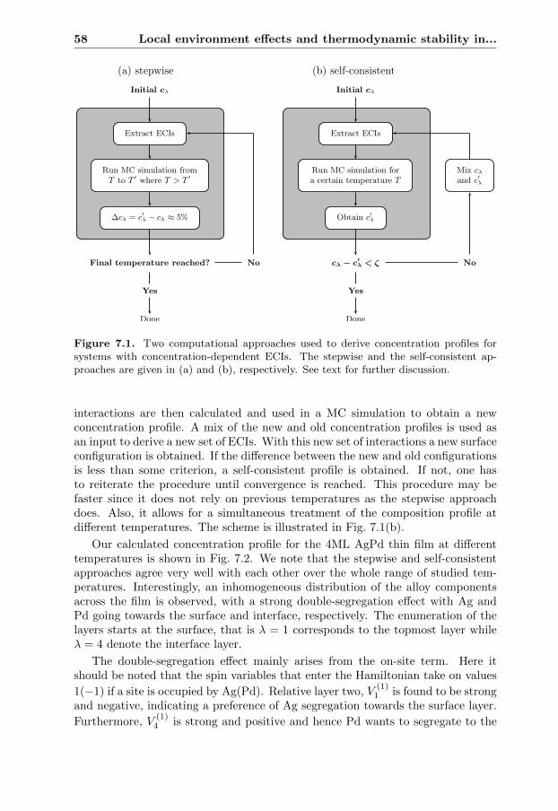
58 Local environment effects and thermodynamic stability in...
(a) stepwise (b) self-consistent
Initial c!
Extract ECIs
Run MC simulation from
T to T!where T > T
!
!c! = c!
! ! c! " 5%
Final temperature reached? No
Yes
Done
Initial c!
Extract ECIs
Run MC simulation for
a certain temperature T
Mix c!
and c!
!
Obtain c!
!
c! ! c!! < ! No
Yes
Done
Figure 7.1. Two computational approaches used to derive concentration profiles forsystems with concentration-dependent ECIs. The stepwise and the self-consistent ap-proaches are given in (a) and (b), respectively. See text for further discussion.
interactions are then calculated and used in a MC simulation to obtain a newconcentration profile. A mix of the new and old concentration profiles is used asan input to derive a new set of ECIs. With this new set of interactions a new surfaceconfiguration is obtained. If the difference between the new and old configurationsis less than some criterion, a self-consistent profile is obtained. If not, one hasto reiterate the procedure until convergence is reached. This procedure may befaster since it does not rely on previous temperatures as the stepwise approachdoes. Also, it allows for a simultaneous treatment of the composition profile atdifferent temperatures. The scheme is illustrated in Fig. 7.1(b).
Our calculated concentration profile for the 4ML AgPd thin film at differenttemperatures is shown in Fig. 7.2. We note that the stepwise and self-consistentapproaches agree very well with each other over the whole range of studied tem-peratures. Interestingly, an inhomogeneous distribution of the alloy componentsacross the film is observed, with a strong double-segregation effect with Ag andPd going towards the surface and interface, respectively. The enumeration of thelayers starts at the surface, that is λ = 1 corresponds to the topmost layer whileλ = 4 denote the interface layer.
The double-segregation effect mainly arises from the on-site term. Here itshould be noted that the spin variables that enter the Hamiltonian take on values
1(−1) if a site is occupied by Ag(Pd). Relative layer two, V(1)1 is found to be strong
and negative, indicating a preference of Ag segregation towards the surface layer.
Furthermore, V(1)4 is strong and positive and hence Pd wants to segregate to the
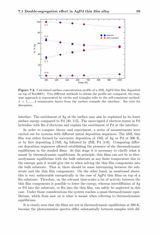
7.1 Double-segregation effect in AgPd thin film alloy 59
300 400 500 600 700 800 900 1000Temp. (K)
0
20
40
60
80
100
At.
% A
g
λ=1
λ=3
λ=2
λ=4
stepwiseself-consistent
Figure 7.2. Calculated surface concentration profile of a 4ML AgPd thin film depositedon top of Ru(0001). Two different methods to obtain the profile are compared, the step-wise approach is represented by circles and triangles refer to the self-consistent method.λ = 1, . . . , 4 enumerates layers from the surface towards the interface. See text fordiscussion.
interface. The enrichment of Ag at the surface may also be explained by its lowersurface energy compared to Pd [40, 115]. The unoccupied d electron states in Pdhybridize with Ru d electrons and explain the enrichment of Pd at the interface.
In order to compare theory and experiment, a series of measurements werecarried out for systems with different initial deposition sequences. The 4ML thinfilm was either formed by successive deposition of 1ML of Ag or Pd at 300 K,or by first depositing 2.1ML Ag followed by 2ML Pd [116]. Comparing differ-ent deposition sequences allowed establishing the presence of the thermodynamicequilibrium in the studied films. At this stage it is necessary to clarify what ismeant by thermodynamic equilibrium. In principle, thin films can not be in ther-modynamic equilibrium with the bulk substrate at any finite temperature due tothe entropy gain it would give rise to when solving the thin film components intothe bulk substrate. That is, there should be some intermixing between the sub-strate and the thin film components. On the other hand, as mentioned above,this is very unfavorable energetically in the case of AgPd thin films on top of aRu substrate. Therefore, on the relevant time-scales a lot of activity between thethin film components is possible to lower the energy, whereas interdiffusion of Agor Pd into the substrate, or Ru into the thin film, can safely be neglected in thiscase. Under those considerations the system reaches a quasi-thermodynamic equi-librium, which from now on is what is meant when referring to thermodynamicequilibrium.
It is clearly seen that the films are not in thermodynamic equilibrium at 300 K,because the photoemission spectra differ substantially between samples with dif-

60 Local environment effects and thermodynamic stability in...
Inte
nsity
(arb
. uni
ts)
Pd(2.0)/Ag(2.1)/RuAg(1)/Pd(1)/Ag(1)/Pd(1)/RuPd(1)/Ag(1)/Pd(1)/Ag(1)/Ru
-12 -11 -10 -9 -8 -7 -6 -5 -4 -3 -2 -1 0 1E-EF [eV]
0
20
40
60
80
100
120
DO
S [s
tate
s·(Ry
·ato
m)-1
]
λ=1λ=2Total
660 K
Homogenous film
(a)
(b)
300 K
660 K
645 K
650 KDOS(states/(R
y·atom
))
E ! Ef (eV)
Intensity
(arb.units)
(a)
(b)
Figure 7.3. (a) Experimental valence band spectra at different temperatures for thethree differently initially prepared thin films. The deposition sequence is indicated in thelegend. (b) Theoretical layer resolved valence band density of states and total DOS. Thetotal DOS is calculated according to Eq. (7.9). The DOS at 660 K is obtained from thetheoretically determined surface concentration profile and the DOS for a homogeneousfilm is presented for comparison. The figure is taken from Paper VII.
ferent initial deposition sequences as seen in Fig. 7.3(a). The legend shows thedeposition sequence for the differently prepared thin films. The pronounced differ-ence between the valence band (VB) spectra of the Ag respectively Pd terminatedsamples at 300 K reveals the presence of Pd at the surface in the latter sam-ples. On the contrary, at around 650 K the VB spectra from different samples aremuch closer to each other, indicating that they are very close to thermodynamicequilibrium. All spectra exhibit a strong dominant Ag contribution at higher tem-peratures, irrespective of the initial preparation. This supports the theoreticalprediction of the absence of Pd in the surface layer.
Theoretical valence-band density of states (VB-DOS) for the concentrationprofile obtained at 660 K is shown in Fig.7.3(b). Good agreement to experiment isfound as regards the width of the band, the peak alignments as well as the shoulderclose to the Fermi level, which originates from deeper layers as seen from the layer-resolved DOS. The total VB-DOS is calculated from the following equation
gtot =
4∑
λ=1
wλ · g(λ), (7.9)

7.1 Double-segregation effect in AgPd thin film alloy 61
concentration profile of the alloy surface. One could expectthat this ordering tendency increases in the thin film, becausethe observed double-segregation effect provides naturalboundary conditions to form an ordered sequence of alternat-ing Ag and Pd layers similar to a stacking of !111" planes inthe L11 structure. However, Fig. 3 shows that this does nothappen. Note that if one is not careful, one might think thatthe concentration profiles for the film and for the alloy sur-face are the same or very similar to each other. But as amatter of fact, the segregation profiles are qualitatively dif-ferent between the surface of the alloy and the alloy film, aslayers 2 and 4 are interchanged in Fig. 4, as compared to Fig.3. This indicates that the surface-induced ordering of the L11type, present at the alloy surface, is suppressed in the film. Ifwe compare the same pair interactions as above for the filmat 550 K !in mRy" !V11;1=2.66, V12;1=3.20, V12;2=1.45;V22;1=1.00, V23;1=1.10, V23;2=0.91; V33;1=0.28, V34;1=!0.48, V34;2=0.40", we observe that the interactions aredamped through the layers and that the NN interlayer inter-action V34;1 even changes sign. We conclude that the nano-scale thickness of the Ag-Pd alloy film is essential for theordering behavior of the system, which differs drasticallyboth from the bulk systems with complete solubility between
Ag and Pd and from the surfaces of bulk alloys with a strongtendency toward L11-surface-induced order.
B. Comparison to experiment
In order to compare theory and experiment, thin Ag-Pdfilms were deposited on a Ru!0001" substrate and the coreand valence band !VB" spectra were studied by photoelec-tron spectroscopy. Experimental data are based on the use ofsynchrotron radiation, from the storage ring ISA at AarhusUniversity, for measurements of the core-level shifts !CLSs"of the 3d5/2 electrons of Ru, Pd, and Ag. The photon energywas 40 eV for excitation of valence band electrons. Thebeamline is equipped with a spherical grating monochro-mator and a SCIENTA hemispherical concentric analyzer.Photons were incident at an angle of 40° with respect to thesurface normal, and photoelectrons were collected by the200-mm-mean-radius energy analyzer along the surface nor-mal. The opening angle of the analyzer was !9° and thetotal instrumental resolution was better than 0.2 eV and0.1 eV for the 3d5/2 core electrons and valence band elec-trons, respectively. It was ensured that the kinetic energies ofthe emitted 3d electrons, around 60 eV, correspond to infor-mation from the first three to four atomic layers according tothe exponential decay of the intensity with increasing depth.The facilities of the end station and the preparation of theRu!0001" surface have been described earlier in Ref. 44.Calibrations of the Ag and Pd evaporation sources werebased on photoelectron intensities, CLSs, and variations inthe full widths at half maximum !FWHMs". The evaporationrate was in the order of 0.14 monolayers /min. Concerningthe geometrical structure, low-energy electron diffraction!LEED" demonstrated the hexagonal patterns from the over-layers.
The 4-ML-thick AgxPd1!x binary alloy film of the nomi-nal composition Ag50Pd50 was formed by successive deposi-tion of 1 ML of either Ag or Pd at 300 K on the Ru!0001"surface. In order to ensure that the films were as close aspossible to the thermodynamic equilibrium extended anneal-ing periods, of 30 min duration for temperatures below
Inte
nsity
(arb
.uni
ts)
Pd(2.0)/Ag(2.1)/RuAg(1)/Pd(1)/Ag(1)/Pd(1)/RuPd(1)/Ag(1)/Pd(1)/Ag(1)/Ru
-12 -11 -10 -9 -8 -7 -6 -5 -4 -3 -2 -1 0 1E-EF [eV]
0
20
40
60
80
100
120
DO
S[s
tate
s/(R
y*at
om)]
!=1!=2Total
660 K
Homogenous film
(a)
(b)
300 K
660 K
645 K
650 K
FIG. 5. !Color online" Comparison between !a" experimentalvalence band !VB" spectra and !b" theoretical VB density of states!DOS". !a" VB spectra of the Pd!2.0"/Ag!2.1"/Ru, Ag!1"/Pd!1"/Ag!1"/Pd!1"/Ru, and Pd!1"/Ag!1"/Pd!1"/Ag!1"/Ru interfaces at indi-cated temperatures. !b" Calculated layer-resolved VB-DOS for thesurface and the subsurface layers as well as the total VB-DOS,which corresponds to the contribution from all layers accounting forthe attenuation in the intensity through the layers—i.e., #"=1
4 w"
#DOS!"". The attenuation factor w" takes on values 1.00, 0.57,0.33, and 0.19 for layers 1, 2, 3, and 4, respectively, and DOS!""denotes the calculated VB-DOS in layer ".
278 278.5 279 279.5 280 280.5 281 281.5 282Binding energy [eV]
Inte
nsity
(arb
.uni
ts)
Clean Ru(0001) surface at 300 KAg(1.3)/Ru(0001) at 400 KPd(1.3)/Ru(0001) at 400 KPd(1)/Ag(1)/Pd(1)/Ag(1)/Ru(0001)after annealing at 645 K
FIG. 6. !Color online" Ru 3d5/2 core level spectra recorded foran incoming photon energy of 350 eV. See text for discussion.
MARTEN et al. PHYSICAL REVIEW B 77, 125406 !2008"
125406-4
Intensity
(arb.units)
Binding energy (eV)
Figure 7.4. Experimental Ru3d5/2 core level spectra for dif-ferent films. The figure is takenfrom Paper VII.
where g(λ) is the layer resolved DOS and wλ is the attenuation factor through thelayers. Explicit numbers of wλ are found in Paper VII. In particular, the film withoriginal deposition sequence Ag(1)/Pd(1)/Ag(1)/Pd(1)/Ru is in best agreementwith theory. Among the initially different samples, this is actually the thin filmwhich is closest to the predicted equilibrium profile. This confirms the theoreticalprediction of Ag enrichment at the surface layer.
Furthermore, the theoretical prediction of Pd at the interface with Ru is sup-ported by experimental binding energy spectra of the Ru 3d5/2 core-level, shown inFig. 7.4. Among the three possible interfaces included in the figure, the Ru 3d5/2
spectrum from the Pd(1)/Ag(1)/Pd(1)/Ag(1)/Ru sample after annealing at 645 Kfits with the Ru 3d5/2 core-level spectrum recorded for the Pd(1.3)/Ru interface.This indicates that the local chemical environment around Ru atoms mainly iscomposed of Pd atoms, and supports the theoretical conclusion of the segregationof Pd towards the interface with Ru.
Another interesting phenomenon while decreasing the temperature is the ob-served tendency to form alternating layers in the thin film. This correspondsto L11 ordering, i.e. alternating layers in the fcc (111) or hcp (0001) direction,which is observed at surfaces of AgPd alloys close to the equiatomic composi-tion [112, 117, 118, 119, 120, 121]. To illustrate the difference in ordering betweenthe thin alloy film and the alloy surface, a self-consistent concentration profile forthe (111) surface of Ag50Pd50 was derived. This was achieved employing the sametheoretical technique as for the thin film alloy above. Although exchange of atomsbetween bulk and surface was permitted, the result in Fig. 7.5 quantitatively de-scribes the composition profile at the Ag50Pd50 surface. Nevertheless, up to 600 Ksurface induced ordering takes place with Ag segregating to the surface and Pd tothe subsurface. At lower temperatures the third and the fourth layer are enrichedby Ag and Pd respectively. One would expect that the double-segregation effectobserved in the thin film should enhance this ordering behaviour since it providesnatural boundary conditions to forming an ordered sequence of alternating Ag andPd layers similar to a stacking of (111) planes in the L11 structure. Interestinglythough if one compares Fig. 7.2 and Fig. 7.5 one concludes that in the thin AgPd
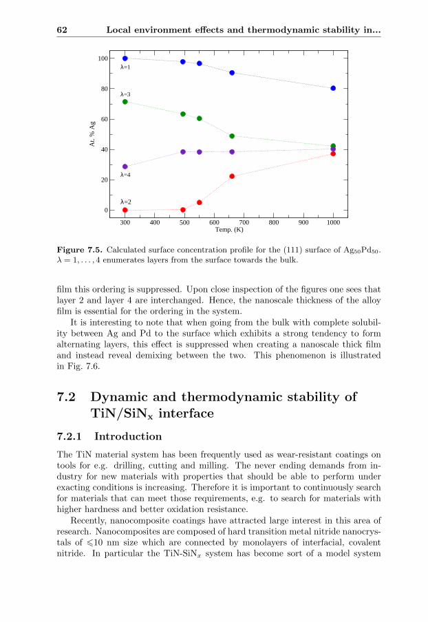
62 Local environment effects and thermodynamic stability in...
300 400 500 600 700 800 900 1000Temp. (K)
0
20
40
60
80
100
At.
% A
g
λ=1
λ=3
λ=4
λ=2
Figure 7.5. Calculated surface concentration profile for the (111) surface of Ag50Pd50.λ = 1, . . . , 4 enumerates layers from the surface towards the bulk.
film this ordering is suppressed. Upon close inspection of the figures one sees thatlayer 2 and layer 4 are interchanged. Hence, the nanoscale thickness of the alloyfilm is essential for the ordering in the system.
It is interesting to note that when going from the bulk with complete solubil-ity between Ag and Pd to the surface which exhibits a strong tendency to formalternating layers, this effect is suppressed when creating a nanoscale thick filmand instead reveal demixing between the two. This phenomenon is illustratedin Fig. 7.6.
7.2 Dynamic and thermodynamic stability ofTiN/SiNx interface
7.2.1 Introduction
The TiN material system has been frequently used as wear-resistant coatings ontools for e.g. drilling, cutting and milling. The never ending demands from in-dustry for new materials with properties that should be able to perform underexacting conditions is increasing. Therefore it is important to continuously searchfor materials that can meet those requirements, e.g. to search for materials withhigher hardness and better oxidation resistance.
Recently, nanocomposite coatings have attracted large interest in this area ofresearch. Nanocomposites are composed of hard transition metal nitride nanocrys-tals of 610 nm size which are connected by monolayers of interfacial, covalentnitride. In particular the TiN-SiNx system has become sort of a model system
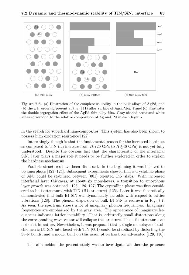
7.2 Dynamic and thermodynamic stability of TiN/SiNx interface 63
(b) alloy surface
Ag
Pd
(a) bulk alloy
Ag
Pd
!=1
!=2
!=3
!=4
(c) thin alloy film
Ru
Figure 7.6. (a) Illustration of the complete solubility in the bulk alloys of AgPd, and(b) the L11 ordering present at the (111) alloy surface of Ag50Pd50. Panel (c) illustratesthe double-segregation effect of the AgPd thin alloy film. Gray shaded areas and whiteareas correspond to the relative composition of Ag and Pd in each layer λ.
in the search for superhard nanocomposites. This system has also been shown topossess high oxidation resistance [122].
Interestingly though is that the fundamental reason for the increased hardnessas compared to TiN (an increase from H≈20 GPa to H&40 GPa) is not yet fullyunderstood. Despite the obvious fact that the characteristic of the interfacialSiNx layer plays a major role it needs to be further explored in order to explainthe hardness mechanism.
Possible structures have been discussed. In the beginning it was believed tobe amorphous [123, 124]. Subsequent experiments showed that a crystalline phaseof SiNx could be stabilized between (001) oriented TiN slabs. With increasedinterfacial layer thickness, at about six monolayers, a transition to amorphouslayer growth was obtained. [125, 126, 127] The crystalline phase was first consid-ered to be isostructural with TiN (B1 structure) [125]. Later it was theoreticallydemonstrated that bulk B1 SiN was dynamically unstable with respect to latticevibrations [128]. The phonon dispersion of bulk B1 SiN is redrawn in Fig. 7.7.As seen, the spectrum shows a lot of imaginary phonon frequencies. Imaginaryfrequencies are emphasized by the gray area. The appearance of imaginary fre-quencies indicates lattice instability. That is, arbitrarily small distortions alongthe corresponding wave-vector will collapse the structure. Thus, the structure cannot exist in nature. Nevertheless, it was proposed that a single monolayer of stoi-chiometric B1 SiN interfaced with TiN (001) could be stabilized by distorting theSi–N bonds, and a model built on this assumption has been advocated [129, 130].
The aim behind the present study was to investigate whether the presence

64 Local environment effects and thermodynamic stability in...
KX! ! X WL L
30
20
10
0
-10i
Freq
uenc
y(THz)
B1 SiNB1 SiN
KX! ! X WL L
30
20
10
0
-10i
Frequ
ency
(THz)
Figure 7.7. Calculated phononspectrum for B1 SiN. Thegray area emphasizes imaginaryfrequencies. Redrawn fromRef. [128].
of TiN interfaces changes the dynamical stability of SiN and to systematicallyinvestigate if the structural model [129, 130] is realistic. This was tested explicitlyby calculating phonon dispersion relations, which reveals the dynamical stabilityof the structures. The theoretical methodology on how to do this is briefly outlinedin the next section. Furthermore, the stability upon formation of Si vacancies wascarried out by relaxing the compositional degree of freedom at the interfacial layer.In this particular study a single monolayer of SiNx interfaced with B1 TiN(001)and TiN(111) were under investigation, the ideal structures are given in Fig. 7.8.
7.2.2 Lattice dynamics
In a crystal the ions vibrate around their equilibrium positions. Within the Born-Oppenheimer approximation the vibrations of the nuclei are decoupled from theelectronic degrees of freedom. Hence, the equations of motion of the nuclei aresolely determined from the ground state energy of a system of interacting electronsmoving in the field of fixed nuclei. Given the positions of the nuclei {R} the totalenergy E(R) may be derived, recalling Eq. (2.2) and the discussion about theBorn-Oppenheimer approximation. Classically, Newton’s equation of motion ofion i with mass Mi can be written as [4]
Mi∂2Ri
∂t2= Fi = −∂E(R)
∂Ri. (7.10)
If small atomic displacements from equilibrium positions are assumed, a Taylorexpansion of the total energy around the average positions {R0} may be carriedout. Furthermore, in the so-called harmonic approximation, vibrational modes ofthe following form are assumed [4]
uieiωt = Ri(t)−R0
i . (7.11)
Thus, carrying out the expansion of the energy and assuming displacements asgiven above, then inserting the results into the equation of motion yields for everyion i that [4]
− ω2Miui,α = −∑
j,β
Ci,α;j,βuj,β , (7.12)

7.2 Dynamic and thermodynamic stability of TiN/SiNx interface 65
Ti
Si
N
Figure 7.8. A single monolayer of SiNinterfaced with B1 TiN(001) (left) andTiN(111) (right).
where the so-called force constants are defined as
Ci,α;j,β =∂2E(R)
∂Ri,α∂Rj,β. (7.13)
The force constants connect a displacement of atom j to the force exerted on atomi. In deriving Eq. (7.12) the linear order term in the expansion of the total energyvanishes, since all derivatives should be evaluated at equilibrium positions with nonet force on any ion. The first non-vanishing correction to the equilibrium energyis thus the second order term. Higher order terms are referred to as anharmoniccontributions and have in this particular study been left out. α and β denotecartesian components and will in the following be suppressed for transparency.
If ui is rescaled to√Miui and given the fact that Eq. (7.12) should be valid
for each ion i the full spectra of vibrational frequencies ω can be determined bythe secular equation
det
(1√MiMj
∂2E(R)
∂Ri∂Rj− ω2
)= 0. (7.14)
Thus, in order to obtain the vibrational frequencies an evaluation of the secondderivative of the total energy is necessary.
Recalling the Hellmann-Feynman theorem, Section 4.5, the force Fi acting onion i with mass Mi could be written as
Fi = −∂E(R)
∂Ri= −
∫n(r)
∂Vext(r)
∂Ridr − ∂Eion-ion
∂Ri, (7.15)
where n(r) is the ground state electron density for the given ionic configuration.Thus, the force constants are obtained by differentiating the Hellmann-Feynmanforces
∂2E(R)
∂Ri∂Rj=
∫∂n(r)
∂Rj
∂Vext(r)
∂Ridr +
∫n(r)
∂2Vext(r)
∂Ri∂Rjdr +
∂2Eion-ion
∂Ri∂Rj. (7.16)

66 Local environment effects and thermodynamic stability in...
(a) (b)
Γ X M Γ Z R A-10i
-5i
0
5
10
15
20Fr
eque
ncy
(TH
z)
Γ K M Γ A0
5
10
15
20
25
Freq
uenc
y (T
Hz)
Figure 7.9. Calculated phonon spectra of the (a) (001) and (b) (111) interfaces for thecase when the atoms occupy ideal in-plane B1 positions, though statically relaxed in thedirection normal to the interfaces. Figures are taken from Paper VIII.
Hence, in order to derive the force constants and in turn the phonon spectrum theknowledge about the ground state density n(r) and its response to a distortion∂n(r)/∂Rj is required. The response of the charge density can be obtained bylinearizing Eqs. (2.8), (2.9), and (2.14), yielding a set of equations that can besolved self-consistently. The derivation of the linear response upon distortion ofthe ions is left out but can be found in the literature [4, 52, 131].
Also the supercell approach to derive the force constants should be mentionedin this context. Within this method, also referred to as the direct method or thesmall displacement method, the idea is to make small distortions in the atomicpositions and calculate the induced force. The drawback with this method is thatone has to introduce supercells opposed to the linear response method where thederivation of the spectra is carried out in the unit cell [52]. For certain systems theforce constants can be long-ranged and hence large supercells are required. [132]
The phonon dispersions of the TiN/SiNx interfaces were studied utilizing theharmonic approximation to the force constants as well as the linear responsemethod as implemented in quantum-espresso [26]. For a detailed derivationof all equations and the realization in the framework of pseudopotentials, the re-view by Baroni et al. [52] is suggested. Moreover, ultrasoft pseudopotentials thathave been shown to give results in good agreement with experiment as well as toother theoretical methods were used [133, 134].
7.2.3 Evaluation of the stability
To study the possible dynamical stabilization of SiN by introducing TiN interfacesthe phonon frequencies were calculated. Figure 7.9 show the calculated spectrafor the case when the atoms occupy ideal in-plane B1 lattice positions (atomsare only relaxed in the direction normal to the interface plane). Compared tothe phonon dispersion in bulk B1 SiN, given in Fig. 7.7, the (001) interface stillexhibits branches which have imaginary phonon frequencies. Interestingly, in the
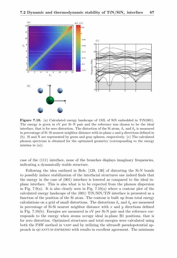
7.2 Dynamic and thermodynamic stability of TiN/SiNx interface 67
x
y
(a)
(b)
0 2 4 6 8 10 12 140
2
4
6
8
10
12
14
!x
! y
"0.24
"0.2
"0.16
"0.12
"0.08
"0.04
0
0.04
#E !eV"
!x
!y
!E (eV)
Z Γ X Y Γ R-5i
0
5
10
15
20
25
Freq
uenc
y (T
Hz)
(c)
Figure 7.10. (a) Calculated energy landscape of 1ML of SiN embedded in TiN(001).The energy is given in eV per Si–N pair and the reference was chosen to be the idealinterface, that is for zero distortion. The distortion of the Si atom, δx and δy is measuredin percentage of Si–Si nearest neighbor distance with in-plane x and y directions defined in(b). Si and N are represented by green and gray spheres, respectively. (c) The calculatedphonon spectrum is obtained for the optimized geometry (corresponding to the energyminima in (a)).
case of the (111) interface, none of the branches displays imaginary frequencies,indicating a dynamically stable structure.
Following the idea outlined in Refs. [129, 130] of distorting the Si-N bondsto possibly induce stabilization of the interfacial structures one indeed finds thatthe energy in the case of (001) interface is lowered as compared to the ideal in-plane interface. This is also what is to be expected from the phonon dispersionin Fig. 7.9(a). It is also clearly seen in Fig. 7.10(a) where a contour plot of thecalculated energy landscape of the (001) TiN/SiN/TiN interface is presented as afunction of the position of the Si atom. The contour is built up from total energycalculations on a grid of small distortions. The distortions δx and δy are measuredin percentage of Si-Si nearest neighbor distance with x and y directions definedin Fig. 7.10(b). Energies are measured in eV per Si-N pair and the reference cor-responds to the energy when atoms occupy ideal in-plane B1 positions, that isfor zero distortion. Optimized structures and total energies were calculated usingboth the PAW method in vasp and by utilizing the ultrasoft pseudopotential ap-proach in quantum-espresso with results in excellent agreement. The minimum

68 Local environment effects and thermodynamic stability in...
is found at approximately 10% distortion along either, due to symmetry, the x orthe y axis.
On the other hand, for the (111) interface, similar distortions only result inrelaxation in the z-direction, i.e. the lowest energy is found for in-plane ideal po-sitions. This actually corresponds to the structure for which the phonon spectrumin Fig. 7.9(b) is obtained.
The calculated phonon dispersion for the geometry that minimizes the energyfor the case of the (001) interface is shown in Fig. 7.10(c). One notices thatimaginary frequencies still appear even though the structure was allowed to relaxinto the energy minimum by distorting the bonds. However, the number of phononbranches showing imaginary frequencies are significantly reduced. Nevertheless,imaginary frequencies suggest that the particular structure is unstable, at least atlow temperatures. At the same time, given the small imaginary part, it may bestabilized by anharmonic effects with increased temperature [135].
The local environment effect of TiN interfaces is illuminated by the absenceof imaginary phonon frequencies and a great reduction of the same in the case of(111) and (001) interfaces, respectively.
To further test the structural model the stoichiometric degree of freedom wasrelaxed allowing for silicon vacancies at the interface. The vacancy formation en-ergy with respect to a Si atom in bulk Si was in actual calculations simulated byremoval of one Si atom of totally four, resulting in a Si3N4 interfacial stoichiometry.All energies were obtained at optimized geometries. We find large and negativevalues for both interfaces (-1.59 eV and -0.65 eV for the case of (001) and (111)interface, respectively). This actually means that there is a preference of spon-taneous creation of Si vacancies. Hence both structures are thermodynamicallyunstable with respect to formation of Si vacancies. Furthermore, Hao et al. [136]noted that the stoichiometric degree of freedom is of importance and also provedthat there are other chemical potentials apart from the one used above that aremore energetically favorable, regardless if the structure is grown under nitrogenpoor or rich conditions. Thus, the derived vacancy formation energies are under-estimations and an enhancement of the driving force of forming vacancies is to beexpected.
Even though the presence of TiN interfaces has a stabilization effect on thelattice dynamics, the results above suggest that in seeking for possible structure ofTiN/SiNx, stoichiometries other than 1:1 between Si and N should be considered.Possible structures with 3:4 ratio of Si to N stoichiometry that are dynamicallystable in bulk and with well matched lattice parameters to TiN have been pointedout in Ref. [128]. These structures seem promising but a verification similar toabove is required.

CHAPTER 8
Conclusions
The aim with this thesis has been to study the local environment effects presentin alloys. Observable physical properties have been calculated to illuminate theimportance of the effect. The effect of local environments on physical propertiesin the bulk, in magnetic systems, as well as in inhomogeneous systems have beenstudied.
The presence of local environment effects in equiatomic random alloys washighlighted by calculating the core-level binding energy shifts for every atom inlarge supercells. The results demonstrate that there are different contributions tothe disorder broadening that vary with the local chemical environments. Initialstate and final state contributions can either cancel or reinforce each other toadditionally broaden the photoemission spectra. The latter effect is observed inthe case of Ag and Cu, the final state contribution additionally increases thedisorder broadening. On the contrary, in the case of Pd, and particularly in CuPd,a cancellation among the two contributions is observed with the result of a narrowdisorder broadening.
Inhomogeneous lattice distortions were demonstrated to be of importance whensystems with large size-mismatch between the constituent atoms are under con-sideration. It was shown that the effect of local lattice relaxations both couldincrease and reduce the disorder broadening. The latter effect is observed for bothcomponents in random equiatomic CuAu alloy. For instance, in the case of Cu thesuppression of disorder broadening is so strong that the disorder broadening effectis below the experimental detection limit. Theoretically this was explained by adelicate balance between the dispersion of the core-level shifts, induced by differentlocal environments, and the influence of inhomogeneous lattice distortions.
Opposed to the disorder broadening of core-level binding energy shifts in theequiatomic AgPd alloy, both components show identical disorder broadening ofAuger kinetic energy shifts. The disorder broadening of Auger parameter shifts
69

70 Conclusions
was found to be significantly broader in the case of Pd as compared to Ag. For Agboth the disorder broadening and the mean value are close to zero. This reveals theimportance of final state effect in the case of Pd and an almost zero contributionin the case of Ag.
In conclusion, a robust theoretical framework for calculating disorder broaden-ing of core levels has been developed.
The local environment effects on physical properties in a magnetic system wasstudied in the equiatomic random fcc FeNi alloy. The sensitivity was explicitlyshown by calculating local magnetic moments and exchange parameters at differentchemical environments. It was shown that Fe sites in Fe rich local environmentsexhibit stronger tendency towards antiferromagnetism.
A combined theoretical and experimental study of thin AgxPd1−x films on topof Ru substrate was carried out. It was demonstrated that ordering trends inintermetallic alloys can be influenced by reduction of the dimensionality of thealloy system to thin films with nanometer thickness. This was shown by studyingthe concentration profile of the AgPd film. Opposed to the situation in bulkwhere there is a complete solubility between Ag and Pd the alloy components aredistributed non-uniformly across the thin film. A double-segregation effect wasobserved with Ag and Pd showing strong preference towards the surface and theinterface, respectively. The surface induced L11 ordering, i.e. alternating layers ofAg and Pd in the fcc (111) or hcp (0001) direction present at the surface of AgPdalloys around the equiatomic composition, was observed to be weakened due tothe nanometer thickness of the film. Hence, the structural properties of the filmsare much more diverse than their bulk counterparts and their surfaces.
It was considered whether the presence of TiN interfaces changes the stabilityof SiN. In particular two different interfaces were studied: one monolayer SiNx
embedded between B1 TiN (001) and B1 TiN (111). Phonon calculations showedthat the (111) interface is dynamically stable while distortion of the Si-N bondfrom ideal in-plane B1 positions almost, but not completely, stabilizes the (001)interface dynamically. However, both interfaces were found to be unstable withrespect to Si vacancy formation. In conclusion, this mean that the interestingphysical properties of real existing TiN-SiNx nanocomposites can not be under-stood from the calculated properties of isostructural TiN/SiN interfaces with Si1N1
stoichiometry. In order to understand the hardening mechanism and the explana-tion of the experimental finding of epitaxial SiNx in TiN/SiNx multilayers otherstructures with more complicated geometry and other stoichiometries need to beinvestigated.
Bibliography
[1] L. H. Thomas. The calculation of atomic fields. Math. Proc. CambridgePhilos. Soc., 23(05):542–548, 1927.
[2] E. Fermi. Un metodo statistico per la determinazione di alcune priorietadell’atome. Rend. Accad. Naz. Lincei, 6:602, 1927.
[3] P. Hohenberg and W. Kohn. Inhomogeneous Electron Gas. Phys. Rev.,136:B864, 1964.
[4] R. M. Martin. Electronic Structure: Basic Theory and Practical Methods.Cambridge University Press, 2004.
[5] W. Kohn and L. J. Sham. Self-Consistent Equations Including Exchangeand Correlation Effects. Phys. Rev., 140:A1133, 1965.
[6] D. M. Ceperley and B. J. Alder. Ground State of the Electron Gas by aStochastic Method. Phys. Rev. Lett., 45(7):566–569, 1980.
[7] O. Gunnarsson and B. I. Lundqvist. Exchange and correlation in atoms,molecules, and solids by the spin-density-functional formalism. Phys. Rev.B, 13(10):4274–4298, 1976.
[8] S. H. Vosko, L. Vilk, and M. Nusair. Accurate spin-dependent electron liquidcorrelation energies for local spin density calculations: a critical analysis.Can. J. Phys., 58:1200, 1980.
[9] J. P. Perdew and A. Zunger. Self-interaction correction to density-functionalapproximations for many-electron systems. Phys. Rev. B, 23(10):5048–5079,1981.
[10] J. P. Perdew and Y. Wang. Accurate and simple analytic representation ofthe electron-gas correlation energy. Phys. Rev. B, 45(23):13244–13249, 1992.
71

72 Bibliography
[11] U. von Barth and L. Hedin. A local exchange-correlation potential for thespin polarized case: I. J. Phys. C: Solid State Phys., 5(13):1629, 1972.
[12] J. P. Perdew, K. Burke, and M. Ernzerhof. Generalized Gradient Approxi-mation Made Simple. Phys. Rev. Lett., 77:3865, 1996.
[13] A. D. Becke. Density-functional exchange-energy approximation with correctasymptotic behavior. Phys. Rev. A, 38(6):3098–3100, 1988.
[14] Y. Wang and J. P. Perdew. Correlation hole of the spin-polarized electrongas, with exact small-wave-vector and high-density scaling. Phys. Rev. B,44(24):13298–13307, 1991.
[15] J. P. Perdew, J. A. Chevary, S. H. Vosko, K. A. Jackson, M. R. Pederson,D. J. Singh, and C. Fiolhais. Atoms, molecules, solids, and surfaces: Applica-tions of the generalized gradient approximation for exchange and correlation.Phys. Rev. B, 46:6671, 1992.
[16] A. V. Ruban and I. A. Abrikosov. Configurational thermodynamics of al-loys from first principles: effective cluster interactions. Rep. Prog. Phys.,71(4):046501, 2008.
[17] F. Bloch. Uber die Quantenmechanik der Elektronen in Kristallgittern. Z.Physik A, 52(7):555–600, 1928.
[18] N. W. Ashcroft and D. N. Mermin. Solid State Physics. Thomson Learning,1 edition, 1976.
[19] P. E. Blochl. Generalized separable potentials for electronic-structure calcu-lations. Phys. Rev. B, 41(8):5414–5416, 1990.
[20] D. Vanderbilt. Soft self-consistent pseudopotentials in a generalized eigen-value formalism. Phys. Rev. B, 41(11):7892, 1990.
[21] P. E. Blochl. Projector augmented-wave method. Phys. Rev. B, 50:17953,1994.
[22] P. E. Blochl, J. C. Forst, and J. Schimpl. Projector augmented wave method:ab initio molecular dynamics with full wave functions. Bull. Mater. Sci.,26(1):33, 2003.
[23] G. Kresse and D. Joubert. From ultrasoft pseudopotentials to the projectoraugmented-wave method. Phys. Rev. B, 59:1758, 1999.
[24] G. Kresse and J. Furthmuller. Efficiency of ab-initio total energy calculationsfor metals and semiconductors using a plane-wave basis set. Comput. Mater.Sci., 6:15, 1996.
[25] G. Kresse and J. Furthmuller. Efficient iterative schemes for ab initio total-energy calculations using plane-wave basis set. Phys. Rev. B, 54:11169, 1996.
Bibliography 73
[26] P. Giannozzi, S. Baroni, N. Bonini, M. Calandra, R. Car, C. Cavaz-zoni, D. Ceresoli, G. L. Chiarotti, M. Cococcioni, I. Dabo, A. D.Corso, S. de Gironcoli, S. Fabris, G. Fratesi, R. Gebauer, U. Gerst-mann, C. Gougoussis, A. Kokalj, M. Lazzeri, L. Martin-Samos, N. Marzari,F. Mauri, R. Mazzarello, S. Paolini, A. Pasquarello, L. Paulatto, C. Sbrac-cia, S. Scandolo, G. Sclauzero, A. P. Seitsonen, A. Smogunov, P. Umari,and R. M. Wentzcovitch. quantum-espresso: a modular and open-sourcesoftware project for quantum simulations of materials. J. Phys.: Condens.Matter, 21(39):395502, 2009.
[27] J. Korringa. On the calculation of the energy of a Bloch wave in a metal.Physica, 13(6–7):392–400, 1947.
[28] W. Kohn and N. Rostoker. Solution of the Schrodinger Equation in PeriodicLattices with an Application to Metallic Lithium. Phys. Rev., 94:1111, 1954.
[29] J. C. Slater. Wave Functions in a Periodic Potential. Phys. Rev., 51(10):846–851, 1937.
[30] A. Zunger, S.-H Wei, L. G. Ferreira, and J. E. Bernard. Special QuasirandomStructures. Phys. Rev. Lett., 65:353, 1990.
[31] J. M. Sanchez, F. Ducastelle, and D. Gratias. Generalized cluster descriptionof multicomponent systems. Physica A, 128:334, 1984.
[32] J. S. Faulkner. The Modern Theory of Alloys. Prog. Mater. Sci., 27:1, 1982.
[33] P. Soven. Coherent-Potential Model of Substitutional Disordered Alloys.Phys. Rev., 156:809, 1967.
[34] B. L. Gyorffy. Coherent-Potential Approximation for a Nonoverlapping-Muffin-Tin-Potential Model of Random Substitutional Alloys. Phys. Rev.B, 5:2382, 1972.
[35] B. L. Gyorffy, A. J. Pindor, J. Staunton, G. M. Stocks, and H. Winter. Afirst-principles theory of ferromagnetic phase transitions in metals. J. Phys.F: Met. Phys., 15(6):1337–1386, 1985.
[36] P. A. Korzhavyi, A. V. Ruban, I. A. Abrikosov, and H. L. Skriver. Madelungenergy for random metallic alloys in the coherent potential approximation.Phys. Rev. B, 51:5773, 1995.
[37] A. V. Ruban and H. L. Skriver. Screened Coulomb interactions in metallicalloys. I. Universal screening in the atomic-sphere approximation. Phys. Rev.B, 66:024201, 2002.
[38] A. V. Ruban, S. I. Simak, P. A. Korzhavyi, and H. L. Skriver. ScreenedCoulomb interactions in metallic alloys. II. Screening beyond the single-siteand atomic-sphere approximation. Phys. Rev. B, 66:024202, 2002.

74 Bibliography
[39] I. A. Abrikosov and H. L. Skriver. Self-consistent linear-muffin-tin-orbitalscoherent-potential technique for bulk and surface calculations: Cu-Ni, Ag-Pd, and Au-Pt random alloys. Phys. Rev. B, 47:16532, 1993.
[40] A. V. Ruban and H. L. Skriver. Calculated surface segregation in transitionmetal alloys. Comput. Mater. Sci., 15:119, 1999.
[41] I. A. Abrikosov, A. M. N. Niklasson, S. I. Simak, B. Johansson, A. V. Ruban,and H. L. Skriver. Order-N Green’s Function Technique for Local Environ-ment Effects in Alloys. Phys. Rev. Lett., 76:4203, 1996.
[42] I. A. Abrikosov, S. I. Simak, B. Johansson, A. V. Ruban, and H. L. Skriver.Locally self-consistent Green’s function approach to the electronic structureproblem. Phys. Rev. B, 56:9319, 1997.
[43] P. A. Korzhavyi, I. A. Abrikosov, B. Johansson, A. V. Ruban, and H. L.Skriver. First-principles calculation of the vacancy formation energy in tran-sition and noble metals. Phys. Rev. B, 59:11693, 1999.
[44] L. Vitos. Total-energy method based on the exact muffin-tin orbitals theory.Phys. Rev. B, 64(1):014107, 2001.
[45] I. A. Abrikosov, P. A. Korzhavyi, and B. Johansson. Electronic Structureand Physical Properties of Solids: The Uses of the LMTO method. Springer-Verlag Berlin Heidelberg, 2000, pp. 379-398.
[46] Y. Wang, G. M. Stocks, W. A. Shelton, and D. M. C. Nicholson. Order-NMultiple Scattering Approach to Electronic Structure Calculations. Phys.Rev. Lett., 75:2867, 1995.
[47] W. Kohn. Density Functional and Density Matrix Method Scaling Linearlywith the Number of Atoms. Phys. Rev. Lett., 76(17):3168–3171, 1996.
[48] A. V. Ruban, S. I. Simak, S. Shallcross, and H. L. Skriver. Local lattice relax-ations in random metallic alloys: Effective tetrahedron model and supercellapproach. Phys. Rev. B, 67:214302, 2003.
[49] T. Marten, I. A. Abrikosov, W. Olovsson, B. Johansson, R. J. Cole, G. Beam-son, S. R. Haines, and P. Weightman. Suppression of disorder broadeningof core-level photoelectron lines in CuAu alloys by inhomogeneous latticedistortion. Phys. Rev. B, 79(1):012201, 2009.
[50] H. Hellmann. Einfuhrung in die Quantenchemie. Franz Deuticke, Leipzig,1937.
[51] R. P. Feynman. Forces in Molecules. Phys. Rev., 56(4):340–343, 1939.
[52] S. Baroni, S. de Gironcoli, A. Dal Corso, and P. Giannozzi. Phonons andrelated crystal properties from density-functional perturbation theory. Rev.Mod. Phys., 73(2):515–562, 2001.
Bibliography 75
[53] A. Einstein. Uber einen die Erzeugung und Verwandlung des Lichtes betre-ffenden heuristischen Gesichtspunkt. Ann. Physik, 17:132, 1905.
[54] S. Hufner. Photoelectron Spectroscopy: Principles and Applications.Springer-Verlag Berlin, 3 edition, 2003.
[55] I. A. Abrikosov, W. Olovsson, and B. Johansson. Valence-Band Hybridiza-tion and Core Level Shifts in Random Ag-Pd Alloys. Phys. Rev. Lett.,87:176403, 2001.
[56] B. Johansson and N. Martensson. Core-level binding-energy shifts for themetallic elements. Phys. Rev. B, 21:4427, 1980.
[57] A. Rosengren and B. Johansson. Surface heat of segregation from surfacecore-level binding-energy shifts. Phys. Rev. B, 23:3852, 1981.
[58] U. Gelius. Binding Energies and Chemical Shifts in ESCA. Phys. Scr.,9(3):133–147, 1974.
[59] R. J. Cole, N. J. Brooks, and P. Weightman. Madelung Potentials and Dis-order Broadening of Core Photoemission Spectra in Random Alloys. Phys.Rev. Lett., 78:3777, 1997.
[60] R. J. Cole, N. J. Brooks, and P. Weightman. Determination of charge transferin the CuxPd1−x alloy system. Phys. Rev. B, 56:12178, 1997.
[61] W. Olovsson, I. A. Abrikosov, and B. Johansson. Core level shift in ran-dom CuPd and AgPd alloys by the complete screening picture. J. ElectronSpectrosc. Relat. Phenom., 127:65, 2002.
[62] W. Olovsson, C. Goransson, L. V. Pourovskii, B. Johansson, and I. A.Abrikosov. Core-level shifts in fcc random alloys: A first-principles approach.Phys. Rev. B, 72:064203, 2005.
[63] M. Alden, H. L. Skriver, and B. Johansson. Ab initio Surface Core-LevelShifts and Surface Segregation Energies. Phys. Rev. Lett., 71:2449, 1993.
[64] M. Alden, I. A. Abrikosov, B. Johansson, N. M. Rosengaard, and H. L.Skriver. Self-consistent Green’s-function technique for bulk and surface im-purity calculations: Surface core-level shifts by complete screening. Phys.Rev. B, 50:5131, 1994.
[65] A. W. Newton, S. Haines, P. Weightman, and R. J. Cole. Disorder inducedcore photoelectron linewidth broadening in AgPd alloys. J. Electron Spec-trosc. Relat. Phenom., 136:235, 2004.
[66] P. Steiner and S. Hufner. Thermochemical data of alloys from photoelectronspectroscopy. Acta Metall., 29:1885, 1981.

76 Bibliography
[67] P. F. Barbieri, A. de Siervo, M. F. Carazzolle, R. Landers, and G. G.Kleiman. XPS and XAES study of Ag-Pd and Cu-Ni alloys: spectra, shiftsand electronic structure information. J. Electron Spectrosc. Relat. Phenom.,135:113, 2004.
[68] R. J. Cole and P. Weightman. Electrostatics in disordered CuxPd1−x alloys.J. Phys.: Condens. Matter, 10:5679, 1998.
[69] A. W. Newton, A. Vaughan, R. J. Cole, and P. Weightman. Disorder broad-ening of core level photoemission spectra in CuxPt1−x alloys. J. ElectronSpectrosc. Relat. Phenom., 107:185, 2000.
[70] D. Lewis, R. J. Cole, and P. Weightman. Observation of disorder broadeningof core photoelectron spectra of CuZn alloys. J. Phys.: Condens. Matter,11:8431, 1999.
[71] R. J. Cole and P. Weightman. Disorder broadening of core levels: Insightsinto alloy electronic structure. J. Electron Spectrosc. Relat. Phenom., 178–179:112–122, 2010.
[72] J. S. Faulkner, Y. Wang, and G. M. Stocks. Core Level Chemical Shifts inMetallic Alloys. Phys. Rev. Lett., 81:1905, 1998.
[73] B. Drittler, M. Weinert, R. Zeller, and P. H. Dederichs. First-principlescalculation of impurity-solution energies in Cu and Ni. Phys. Rev. B, 39:930,1989.
[74] W. F. Egelhoff. Core-level binding-energy shifts at surfaces and in solids.Surf. Sci. Rep., 6(6-8):253–415, 1987.
[75] J. C. Slater. Quantum theory of molecules and solids, volume 4 of Interna-tional series in Pure and Applied physics. McGraw-Hill, 1 edition, 1974.
[76] J. F. Janak. Proof that ∂E/∂ni = εi in density-functional theory. Phys.Rev. B, 18:7165, 1978.
[77] C. Goransson, W. Olovsson, and I. A. Abrikosov. Numerical investigation ofthe validity of the Slater-Janak transition-state model in metallic systems.Phys. Rev. B, 72(13):134203, 2005.
[78] W. Olovsson, C. Goransson, T. Marten, and I. A. Abrikosov. Core-levelshifts in complex metallic systems from first principle. phys. stat. sol. (b),243:2447, 2006.
[79] W. Olovsson, I. A. Abrikosov, B. Johansson, A. W. Newton, R. J. Cole,and P. Weightman. Auger Energy Shifts in fcc AgPd Random Alloys fromComplete Screening Picture and Experiment. Phys. Rev. Lett., 92:226406,2004.
[80] R. D. Stoker, M. Szmigiel, N. J. Miller, and R. J. Cole. Disorder broadeningof alloy Auger spectra. J. Electron Spectrosc. Relat. Phenom., 162(3):127,2008.
Bibliography 77
[81] M. Prutton. Introduction to Surface Physics. Oxford University Press, USA,2002.
[82] C. D. Wagner. Chemical shifts of Auger lines, and the Auger parameter.Faraday Discuss. Chem. Soc., 60:291–300, 1975.
[83] P. Weightman and R. J. Cole. Electron spectroscopy of disordered metalalloys. J. Electron Spectrosc. Relat. Phenom., 178-179:100–111, 2010.
[84] G. Moretti. Auger parameter and Wagner plot in the characterization ofchemical states by X-ray photoelectron spectroscopy: a review. J. ElectronSpectrosc. Relat. Phenom., 95(2–3):95–144, 1998.
[85] N. Martensson, P. Hedegard, and B. Johansson. Auger Energy Shifts forMetallic Elements. Phys. Scr., 29(2):154–180, 1984.
[86] C. E. Guillaume. Recherches sur les aciers au nickel. Dilatations aux tem-peratures elevees; resistance electrique. C. R. Hebd. Seances. Acad. Sci.,125:235, 1897.
[87] R. J. Weiss. The Origin of the ‘Invar’ Effect. Proc. Phys. Soc., 82(2):281,1963.
[88] M. van Schilfgaarde, I. A. Abrikosov, and B. Johansson. Origin of the Invareffect in iron-nickel alloys. Nature, 400(6739):46–49, 1999.
[89] L. Dubrovinsky, N. Dubrovinskaia, I. A. Abrikosov, M. Vennstrom, F. West-man, S. Carlson, M. van Schilfgaarde, and B. Johansson. Pressure-InducedInvar Effect in Fe-Ni Alloys. Phys. Rev. Lett., 86(21):4851–4854, 2001.
[90] A. V. Ruban, M. I. Katsnelson, W. Olovsson, S. I. Simak, and I. A.Abrikosov. Origin of magnetic frustrations in Fe-Ni Invar alloys. Phys.Rev. B, 71(5):054402, 2005.
[91] F. Liot and C. A. Hooley. Anomalous thermal expansion in iron-basedferromagnets: ab initio calculations and the relation to magnetism. ArXive-prints: 2009arXiv0912.0215L, December 2009.
[92] F. Liot. Thermal Expansion and Local Environment Effects in FerromagneticIron-Based Alloys. PhD thesis, Linkoping University, 2009.
[93] F. Liot and I. A. Abrikosov. Local magnetovolume effects in Fe65Ni35 alloys.Phys. Rev. B, 79(1):014202, 2009.
[94] A. V. Ruban, S. Khmelevskyi, P. Mohn, and B. Johansson. Magnetic state,magnetovolume effects, and atomic order in Fe65Ni35 Invar alloy: A firstprinciples. Phys. Rev. B, 76:014420, 2007.
[95] F. Liot, S. I. Simak, and I. A. Abrikosov. Static ionic displacements in Fe–Nialloys from first principles. J. Appl. Phys., 99(8):08P906, 2006.
78 Bibliography
[96] I. A. Abrikosov, A. E. Kissavos, F. Liot, B. Alling, S. I. Simak, O. Peil, andA. V. Ruban. Competition between magnetic structures in the Fe rich fccFeNi alloys. Phys. Rev. B, 76(1):014434, 2007.
[97] A. I. Liechtenstein, M. I. Katsnelson, and V. A. Gubanov. Exchange inter-actions and spin-wave stiffness in ferromagnetic metals. J. Phys. F: Met.Phys., 14(7):L125, 1984.
[98] A. I. Liechtenstein, M. I. Katsnelson, V. P. Antropov, and V. A. Gubanov.Local spin density functional approach to the theory of exchange interactionsin ferromagnetic metals and alloys. J. Magn. Magn. Mater., 67(1):65–74,1987.
[99] A. I. Liechtenstein, M. I. Katsnelson, and V. A. Gubanov. Local spin excita-tions and Curie temperature of iron. Solid State Commun., 54(4):327–329,1985.
[100] J. Kubler. Theory of Itinerant Electron Magnetism. Oxford University Press,2000.
[101] P. James, O. Eriksson, B. Johansson, and I. A. Abrikosov. Calculated mag-netic properties of binary alloys between Fe, Co, Ni, and Cu. Phys. Rev. B,59(1):419–430, 1999.
[102] J. W. D. Connolly and A. R. Williams. Density-functional theory applied tophase transformations in transition-metal alloys. Phys. Rev. B, 27(8):5169–5172, 1983.
[103] F. Ducastelle. Order and Phase Stability in Alloys. North Holland, Amster-dam, 1991.
[104] F. Ducastelle and F. Gautier. Generalized perturbation theory in disor-dered transitional alloys: Application to the calculation of ordering energies.J. Phys. F: Met. Phys., 6:2039, 1976.
[105] V. Drchal, J. Kudrnovsky, L. Udvardi, P. Weinberger, and A. Pasturel.Effective interatomic interactions in inhomogeneous semi-infinite systems.Phys. Rev. B, 45:14328, 1992.
[106] A. Pasturel, V. Drchal, J. Kudrnovsky, and P. Weinberger. First-principlesstudy of surface segregation in Cu-Ni alloys. Phys. Rev. B, 48:2704, 1993.
[107] V. Drchal, J. Kudrnovsky, A. Pasturel, I. Turek, and P. Weinberger. Ab initiotheory of surface segregation: Self-consistent determination of the concen-tration profile. Phys. Rev. B, 54:8202, 1996.
[108] V. Drchal, A. Pasturel, R. Monnier, J. Kudrnovsky, and P. Weinberger. The-ory of surface segregation in metallic alloys: The generalized perturbationmethod. Comput. Mater. Sci., 15:144, 1999.
Bibliography 79
[109] A. Berera, H. Dreysse, L. T. Willes, and D. de Fontaine. A direct methodfor obtaining effective pair interactions in binary alloys. J. Phys. F: Met.Phys., 18(4):L49, 1988.
[110] H. Dreysse, A. Berera, L. T. Wille, and D. de Fontaine. Determinationof effective-pair interactions in random alloys by configurational averaging.Phys. Rev. B, 39(4):2442–2452, 1989.
[111] A. V. Ruban, S. Shallcross, S. I. Simak, and H. L. Skriver. Atomic andmagnetic configurational energetics by the generalized perturbation method.Phys. Rev. B, 70:125115, 2004.
[112] A. V. Ruban, S. I. Simak, P. A. Korzhavyi, and B. Johansson. Theoreticalinvestigation of bulk ordering and surface segregation in Ag-Pd and otherisoelectronic alloys. Phys. Rev. B, 75:054113, 2007.
[113] T. B. Massalski. Binary Alloy Phase Diagram, volume 2. ASM International,Materials Park, OH, 2nd edition, 1990.
[114] A. V. Ruban, H. L. Skriver, and J. K. Nørskov. Surface segregation energiesin transition-metal alloys. Phys. Rev. B, 59:15990, 1999.
[115] H. L. Skriver and N. M. Rosengaard. Surface energy and work function ofelemental metals. Phys. Rev. B, 46:7157, 1992.
[116] W. Olovsson, L. Bech, T. H. Andersen, Z. Li, S. V. Hoffmann, B. Johansson,I. A. Abrikosov, and J. Onsgaard. Core-level shifts for two- and three-dimensional bimetallic PdxCu1−x and PdxAg1−x alloys on Ru(0001). Phys.Rev. B, 72:075444, 2005.
[117] S. Muller and A. Zunger. First-Principles Predictions of Yet-Unobserved Or-dered Structures in the Ag-Pd Phase Diagram. Phys. Rev. Lett., 87:165502,2001.
[118] M. Ropo, K. Kokko, L. Vitos, and J. Kollar. Segregation at the PdAg(111)surface: Electronic structure calculations. Phys. Rev. B, 71(4):045411, 2005.
[119] M. Ropo, K. Kokko, L. Vitos, J. Kollar, and B. Johansson. The chemi-cal potential in surface segregation calculations: AgPd alloys. Surf. Sci.,600(4):904–913, 2006.
[120] M. Ropo. Ab initio study of the geometric dependence of AgPd surfacesegregation. Phys. Rev. B, 74:195401, 2006.
[121] P. T. Wouda, M. Schmid, B. E. Nieuwenhuys, and P. Varga. STM study ofthe (111) and (100) surfaces of PdAg. Surf. Sci., 417(2–3):292, 1998.
[122] S. Veprek, M. G. J. Veprek-Heijman, P. Karvankova, and J. Prochazka.Different approaches to superhard coatings and nanocomposites. Thin SolidFilms, 476(1):1–29, 2005.

80 Bibliography
[123] S. Veprek and S. Reiprich. A concept for the design of novel superhardcoatings. Thin Solid Films, 268(1–2):64, 1995.
[124] S. Veprek. The origin of superhardness in TiN/Si3N4 nanocomposites: therole of the interfacial monolayer. High Press. Res., 26(2):119–125, 2006.
[125] L. Hultman, J. Bareno, A. Flink, H. Soderberg, K. Larsson, V. Petrova,M. Oden, J. E. Greene, and I. Petrov. Interface structure in superhard TiN-SiN nanolaminates and nanocomposites: Film growth experiments and abinitio calculations. Phys. Rev. B, 75(15):155437, 2007.
[126] H. Soderberg, M. Oden, J. M. Molina-Aldareguia, and L. Hultman. Nanos-tructure formation during deposition of TiN/SiNx nanomultilayer films byreactive dual magnetron sputtering. J. Appl. Phys., 97(11):114327, 2005.
[127] H. Soderberg, M. Oden, A. Flink, J. Birch, P. O. A. Persson, M. Beckers,and L. Hultman. Growth and characterization of TiN/SiN(001) superlatticefilms. J. Mater. Res., 22:3255, 2007.
[128] B. Alling, E. I. Isaev, A. Flink, L. Hultman, and I. A. Abrikosov. Metasta-bility of fcc-related Si-N phases. Phys. Rev. B, 78(13):132103, 2008.
[129] R. F. Zhang, A. S. Argon, and S. Veprek. Friedel Oscillations are Limitingthe Strength of Superhard Nanocomposites and Heterostructures. Phys.Rev. Lett., 102(1):015503, 2009.
[130] R. F. Zhang, A. S. Argon, and S. Veprek. Electronic structure, stability, andmechanism of the decohesion and shear of interfaces in superhard nanocom-posites and heterostructures. Phys. Rev. B, 79(24):245426, 2009.
[131] S. Baroni, P. Giannozzi, and E. Isaev. Density-Functional PerturbationTheory for Quasi-Harmonic Calculations. Rev. Mineral. Geochem., 71(1):39–57, 2010.
[132] A. van de Walle and G. Ceder. The effect of lattice vibrations on substitu-tional alloy thermodynamics. Rev. Mod. Phys., 74(1):11–45, 2002.
[133] E. I. Isaev, R. Ahuja, S. I. Simak, A. I. Lichtenstein, Yu. Kh. Vekilov, B. Jo-hansson, and I. A. Abrikosov. Anomalously enhanced superconductivity andab initio lattice dynamics in transition metal carbides and nitrides. Phys.Rev. B, 72(6):064515, 2005.
[134] E. I. Isaev, S. I. Simak, I. A. Abrikosov, R. Ahuja, Yu. Kh. Vekilov, M. I.Katsnelson, A. I. Lichtenstein, and B. Johansson. Phonon related propertiesof transition metals, their carbides, and nitrides: A first-principles study. J.Appl. Phys., 101(12):123519–123519, 2007.
[135] C. Asker, A. B. Belonoshko, A. S. Mikhaylushkin, and I. A. Abrikosov.First-principles solution to the problem of Mo lattice stability. Phys. Rev.B, 77(22):220102(R), 2008.

Bibliography 81
[136] S. Hao, B. Delley, S. Veprek, and C. Stampfl. Superhard Nitride-BasedNanocomposites: Role of Interfaces and Effect of Impurities. Phys. Rev.Lett., 97(8):086102, 2006.

82 Bibliography

List of Publications
[I] Ab initio study of disorder broadening of core photoemissionspectra in random Cu-Pd and Ag-Pd alloysT. Marten, W. Olovsson, S. I. Simak, and I. A. Abrikosov.Phys. Rev. B, 72:054210, 2005.
[II] Local environment effects in random metallic alloysI. A. Abrikosov, T. Marten, and W. Olovsson.in The Science of Complex Alloy Phases, edited by T. B. Massalski andP. E. A. Turchi, TMS (The Minerals, Metals & Materials Society) pp. 87–108, San Francisco, 2005.
[III] Core-level shifts in complex metallic systems from first principleW. Olovsson, C. Goransson, T. Marten, and I. A. Abrikosov.phys. stat. sol. (b), 243:2447, 2006.
[IV] Suppression of disorder broadening of core-level photoelectronlines in CuAu alloys by inhomogeneous lattice distortionT. Marten, I. A. Abrikosov, W. Olovsson, B. Johansson, R. J. Cole,G. Beamson, S. R. Haines, and P. Weightman.Phys. Rev. B, 79:012201, 2009.
[V] First principle calculations of core-level binding energy and Augerkinetic energy shifts in metallic solidsW. Olovsson, T. Marten, E. Holmstrom, B. Johansson, and I. A. Abrikosov.J. Electron Spectrosc. Relat. Phenom., 178–179:88–99, 2010.
[VI] Magnetism in systems with reduced dimensionality and chemicaldisorder: The local environment effectsI. A. Abrikosov, F. Liot, T. Marten, and E. A. Smirnova.J. Magn. Magn. Mater., 300:211, 2006.
83

84 List of Publications
[VII] Double-segregation effect in AgxPd1−x/Ru(0001) thin film nano-structuresT. Marten, O. Hellman, A. V. Ruban, W. Olovsson, C. Kramer,J. P. Godowski, L. Bech, Z. Li, J. Onsgaard, and I. A. Abrikosov.Phys. Rev. B, 77:125406, 2008.
[VIII] Single-monolayer SiNx embedded in TiN: A first-principles studyT. Marten, E. I. Isaev, B. Alling, L. Hultman, and I. A. Abrikosov.Phys. Rev. B, 81:212102, 2010.
Publications not included in the thesis
[IX] Comparison of thermodynamic properties of cubic Cr1−xAlxN andTi1−xAlxN from first-principles calculationsB. Alling, T. Marten, I. A. Abrikosov, and A. Karimi.J. Appl. Phys., 102:044314, 2007.
[X] Questionable collapse of the bulk modulus in CrNB. Alling, T. Marten, and I. A. Abrikosov.Nat. Mater., 9:283–284, 2010.
[XI] Effect of magnetic disorder and strong electron correlations onthe thermodynamics of CrNB. Alling, T. Marten, and I. A. Abrikosov.Accepted for publication in Phys. Rev. B.
[XII] Interface core level shifts as a probe of embedded thin film qualityW. Olovsson, E. Holmstrom, T. Marten, I. A. Abrikosov, andA. M. N. Niklasson.In manuscript.
[XIII] Electronic theory of materials properties: from fundamentalunderstanding towards materials designI. A. Abrikosov, T. Marten, P. Olsson, and S. I. Simak.Snic Progress Report 2003–2005, pp. 140–142.
Comments on Papers
Copyrights of Papers I, IV, VII and VIII belong to American Physical Society.The copyright of Paper II belongs to The Minerals, Metals & Materials Society.Wiley-VCH owns the copyright of Paper III, and the copyrights of Papers V andVI belong to Elsevier. Reprints of the papers are included with permission fromthe copyright holders.
As the first author I have carried out most of the calculations and collaboratedin the analysis and interpretation of the results. I have written the first draft ofthe manuscript, excluding the experimental parts, and has been responsible for theiterative process to the final version. My contribution in Papers II, III, and V are,

List of Publications 85
except from planning, discussions of results and proofreading, the sections relatedto local environment effects. In Paper VI, I contributed with the calculation ofthe density of states at different sites.