theoretical investigation of variable area ejectors -...
TRANSCRIPT
Theoretical Investigation of Variable Area Ejectors
by
Mikhail Koupriyanov
A Thesis submitted to
the Faculty of Graduate Studies and Research
in partial fulfillment of
the requirements for the degree of
Master of Applied Science
Ottawa-Carleton Institute for
Mechanical and Aerospace Engineering
Department of Mechanical and Aerospace Engineering
Carleton University
Ottawa, Ontario, Canada
September 2008
Copyright c©
2008 - Mikhail Koupriyanov
The undersigned recommend to
the Faculty of Graduate Studies and Research
acceptance of the Thesis
Theoretical Investigation of Variable Area Ejectors
Submitted by Mikhail Koupriyanov
in partial fulfillment of the requirements for the degree of
Master of Applied Science
J. Etele, Supervisor
M. I. Yaras, Department Chair
Carleton University
2008
Abstract
A theoretical analysis of a variable area ejector is presented. The flowfield is solved
using a steady quasi-one-dimensional, inviscid control volume formulation for cases
of both complete and incomplete mixing while combustion effects are included with
an equilibrium calculation. An assumed three parameter analytical wall pressure
distribution is used in all cases. Under fully mixed-conditions, the model estimated
compression ratios that were 40% higher than the computational values due to ne-
glecting turbulence and viscosity. This cause was later confirmed with a partially
mixed calculation which also predicted a mixing length of 9 diameters. Under SMC
conditions, improved compression was achieved at an equivalence ratio of 2.5, while
a decrease in performance occurred at Stoichiometric conditions. The oxidation of
carbon monoxide occurred for the entire equivalence ratio range and was responsible
for the majority of the heat release in the ejector. Thrust augmentation was found
to increase with area constriction up to a limit, with the Stoichiometric case yielding
values as high as 12%.
ii

Acknowledgements
My time at Carleton University has been a rewarding and exciting experience which
I will always remember. I would like to extend my thanks to the department faculty
and staff for making me feel welcome in this university which seemed foreign not so
long ago.
I also want to take this opportunity to thank my adviser, Dr. Jason Etele for
giving me the opportunity to work on a challenging and interesting project, which
has greatly extended my understanding of high speed aerodynamics and combustion
(my favorite engineering disciplines). Your guidance and desire to push me to do
better has made me a far more diligent researcher and has greatly improved the
quality of the work which I am now submitting.
Last, but not least, I would like to a acknowledge the Natural Sciences and Engi-
neering Research Council, who’s financial assistance made it possible for me to move
to Ottawa and pursue my Masters degree full time.
iii
Table of Contents
Nomenclature ix
1 Introduction 1
1.1 Background . . . . . . . . . . . . . . . . . . . . . . . . . . . . . . . . 1
1.2 Literature Review . . . . . . . . . . . . . . . . . . . . . . . . . . . . . 4
1.3 Objectives . . . . . . . . . . . . . . . . . . . . . . . . . . . . . . . . . 12
2 Non-Reacting Ejector Theory 14
2.1 Wall Pressure Distribution . . . . . . . . . . . . . . . . . . . . . . . . 19
2.2 Solution for Minimum Rocket Pressure . . . . . . . . . . . . . . . . . 20
2.2.1 Control Volume Solution . . . . . . . . . . . . . . . . . . . . . 21
2.2.2 Riemann Solution . . . . . . . . . . . . . . . . . . . . . . . . . 24
2.3 Wall Pressure Integral . . . . . . . . . . . . . . . . . . . . . . . . . . 28
2.4 Numerical Solution . . . . . . . . . . . . . . . . . . . . . . . . . . . . 30
2.4.1 CV Method - Numerical Solution . . . . . . . . . . . . . . . . 34
2.4.2 Area-Mach Number Relation . . . . . . . . . . . . . . . . . . . 38
3 Theory for SMC Ejector 40
3.1 Gibbs Minimization . . . . . . . . . . . . . . . . . . . . . . . . . . . . 42
3.2 Numerical Solution . . . . . . . . . . . . . . . . . . . . . . . . . . . . 44
iv
TABLE OF CONTENTS
4 Partially Mixed Ejector Theory 51
4.1 Mixed-Flow Velocity Profile . . . . . . . . . . . . . . . . . . . . . . . 54
4.2 Mixing Correlations . . . . . . . . . . . . . . . . . . . . . . . . . . . . 57
4.3 Numerical Solution . . . . . . . . . . . . . . . . . . . . . . . . . . . . 59
5 Results & Discussion 61
5.1 Pressure Distribution . . . . . . . . . . . . . . . . . . . . . . . . . . . 61
5.2 Ejector Performance . . . . . . . . . . . . . . . . . . . . . . . . . . . 65
5.3 Effects of Combustion . . . . . . . . . . . . . . . . . . . . . . . . . . 69
5.4 Effects of Mixing . . . . . . . . . . . . . . . . . . . . . . . . . . . . . 83
5.5 Thrust Augmentation . . . . . . . . . . . . . . . . . . . . . . . . . . . 89
6 Conclusions 94
6.1 Future Work . . . . . . . . . . . . . . . . . . . . . . . . . . . . . . . . 97
v
List of Figures
1.1 Typical RBCC Engine . . . . . . . . . . . . . . . . . . . . . . . . . . 2
1.2 Specific Impulse of Various Propulsive Cycles [17] . . . . . . . . . . . 3
2.1 Ejector Control Volume . . . . . . . . . . . . . . . . . . . . . . . . . 14
2.2 Air & Rocket Control Volumes for Estimating pmin . . . . . . . . . . 21
2.3 Riemann Problem Set-Up Adapted to Ejector . . . . . . . . . . . . . 24
2.4 Velocity Polygon at Node i . . . . . . . . . . . . . . . . . . . . . . . . 26
2.5 Ejector Control Volume showing surface element d~S . . . . . . . . . . 28
2.6 Ejector Solution Process (Non-Reacting) . . . . . . . . . . . . . . . . 33
2.7 CV-based Solution Process for pmin . . . . . . . . . . . . . . . . . . . 37
2.8 Solution of Area-Mach Number Relation . . . . . . . . . . . . . . . . 39
3.1 Ejector Solution Process (Reacting) . . . . . . . . . . . . . . . . . . . 50
4.1 Assumed Velocity Profile at Mixed-Flow Plane . . . . . . . . . . . . . 55
4.2 Velocity Profile at Ejector Inlet . . . . . . . . . . . . . . . . . . . . . 58
5.1 Wall Pressure Distributions . . . . . . . . . . . . . . . . . . . . . . . 62
5.2 Minimum Rocket Stream Pressure at a Fixed Air Mass Flow Rate . . 63
5.3 Ejector Compression Ratio πm, theoretical (dashed lines) and CFD
(solid line) results . . . . . . . . . . . . . . . . . . . . . . . . . . . . . 66
vi
LIST OF FIGURES
5.4 Ejector Compression Augmentation πm, theoretical (dashed lines) and
CFD (solid line) results . . . . . . . . . . . . . . . . . . . . . . . . . . 68
5.5 Ejector Compression Under SMC Conditions . . . . . . . . . . . . . . 71
5.6 Relative Change in Combustion Heat Release (CR = 0.15) . . . . . . 72
5.7 Compression Augmentation at SMC Operation (CR = 0.15) . . . . . 73
5.8 Relative Changes in Pressure and Mach Number (CR = 0.15) . . . . . 74
5.9 Ejector Mixed-Flow Temperature (CR = 0.15) . . . . . . . . . . . . . 75
5.10 Effect of Rocket Temperature on Ejector Compression (CR = 0.15) . . 76
5.11 Ejector Composition - Major Species (CR = 0.15) . . . . . . . . . . . 78
5.12 Ejector Composition - Minor Species (CR = 0.15) . . . . . . . . . . . 80
5.13 Production of CO2 & H2O (CR = 0.15) . . . . . . . . . . . . . . . . . 82
5.14 Momentum Mixing Parameter . . . . . . . . . . . . . . . . . . . . . . 84
5.15 Energy Mixing Parameter . . . . . . . . . . . . . . . . . . . . . . . . 85
5.16 Effect of Ejector Duct Length . . . . . . . . . . . . . . . . . . . . . . 86
5.17 Velocity Profiles at Mixed-Flow Plane for Various L/D’s . . . . . . . 87
5.18 Velocity u∗ from Eq. (4.17) . . . . . . . . . . . . . . . . . . . . . . . 88
5.19 Calculation of Ejector Thrust . . . . . . . . . . . . . . . . . . . . . . 90
5.20 Ejector Performance Map . . . . . . . . . . . . . . . . . . . . . . . . 91
5.21 Thrust Augmentation and Air Entrainment (CR = 0.3) . . . . . . . . 92
vii
List of Tables
5.1 Test Conditions . . . . . . . . . . . . . . . . . . . . . . . . . . . . . . 61
5.2 Comparison of Flow Variables at Point of Maximum Expansion for
poa = 58.7 kPa . . . . . . . . . . . . . . . . . . . . . . . . . . . . . . . 65
5.3 Assumed Product Species . . . . . . . . . . . . . . . . . . . . . . . . 70
5.4 Ejector Configuration . . . . . . . . . . . . . . . . . . . . . . . . . . . 90
viii

Nomenclature
Roman Symbols
A Area
a speed of sound
bi total flow rate
of atomic species i
ci coefficient
Cp specific heat at constant
pressure
CR contraction ratio 1 − Am/Ai
D diameter
f Newton-Raphson functional
g gibbs free energy (molar)
gof gibbs free energy of
formation (molar)
∆HR heat of reaction
h molar enthalpy
h specific enthalpy
ho
f standard heat of
formation (molar)
L length of ejector duct
m mass flow rate
M Mach number
Mc convective Mach number
n unit normal vector
N molar flow rate
na number of distinct
atomic species
nr number of species in
rocket exhaust
ns number of species
p pressure
R gas constant
r radius
Ru universal gas constant
ix
Nomenclature
s turbulent spreading
parameter
sθ turbulent spreading
parameter based on
momentum thickness
T temperature
t time
u streamwise velocity
u1 velocity at upper boundary
of shear layer
u2 velocity at lower boundary
of shear layer
u∗ dimensionless velocity
u2/u1
~V resultant velocity
v radial velocity
Vcs contact surface velocity
W molecular weight
x axial coordinate
Y mass fraction
Greek Symbols
α air/rocket mass flow ratio
βe energy mixing factor
βm momentum mixing factor
γ ratio of specific heats
δ shear layer thickness,
flow angle
ǫ relative shear layer thickness
δm/rm
ζ rocket/air total pressure
ratio, por/p
oa
ηik amount of atomic particle i per
kmol of species k
θ air/rocket specific total
enthalpy ratio
θo initial momentum thickness
λ Lagrange multiplier
µ functional
ν density ratio, ρr/ρa
ξ non-dimensional shear layer
coordinate
x
Nomenclature
πm compression ratio, pom/p
oa
πm compression augmentation
ratio
ρ density
σ rocket exhaust/ejector
inlet area ratio
τ velocity ratio, ur/ua
Υ numerical damping
parameter
Φ thrust augmentation ratio
Fej/Fr
φr equivalence ratio of the
rocket’s combustion chamber
χ functional
Subscripts
2 point of maximum expansion
a air
AM Area-Mach Number relation
CV control volume
DSL dividing streamline
e propelling nozzle exit
i ejector inlet
m mixed flow (ejector exit)
r rocket
ref reference conditions
(273K, 1atm)
w wall
Superscripts
o stagnation conditions
∗ sonic conditions
− area-averaged quantity
˜ normalized by RuTm
xi
Chapter 1
Introduction
1.1 Background
Currently the only available means of orbital insertion is by using chemical rocket
engines. Although rocket propulsion offers a high thrust-to-weight ratio, it suffers
from a relatively low specific impulse (on the order of 300s), as well as the burden of
having to carry a large quantity of on-board oxidizer. These shortcomings collectively
make launching payloads into space a very expensive endeavour with costs on the
order of $22000/kg of payload. The desire to bring down these costs served as the
impetus behind the Highly Reusable Space Transportation Study released by NASA in
1997. The goal of the study was to identify technologies which would reduce the costs
of space access by a significant amount. Among the candidates which showed promise
of achieving the cost reduction goal were various types of air-breathing Combined-
Cycle Propulsion (CCP) systems. A combined cycle engine essentially integrates
different propulsive cycles into a single engine/flowpath architecture. One of the
variants of such a system is the Rocket-Based Combined-Cycle Engine (RBCC) which
has at its core a chemical rocket, required for space flight and static thrust. An
example of a generic RBCC engine is shown in Figure 1.1.
1
Chapter 1. Introduction
Fuel Fuel
Oxidizer
Inlet Section Ejector/Mixing Section Combustor Nozzle
Annular Rocket MotorFlame Holders
Fuel Injectors
Entrained Air
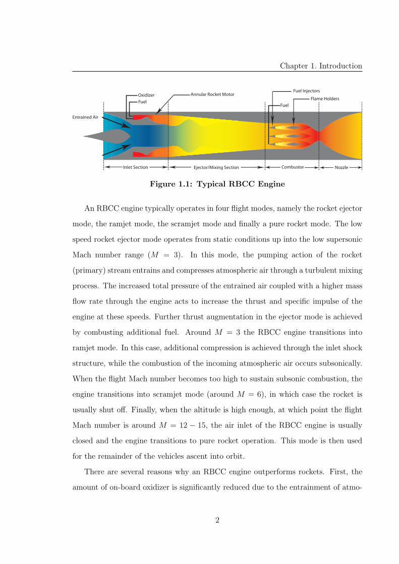
Figure 1.1: Typical RBCC Engine
An RBCC engine typically operates in four flight modes, namely the rocket ejector
mode, the ramjet mode, the scramjet mode and finally a pure rocket mode. The low
speed rocket ejector mode operates from static conditions up into the low supersonic
Mach number range (M = 3). In this mode, the pumping action of the rocket
(primary) stream entrains and compresses atmospheric air through a turbulent mixing
process. The increased total pressure of the entrained air coupled with a higher mass
flow rate through the engine acts to increase the thrust and specific impulse of the
engine at these speeds. Further thrust augmentation in the ejector mode is achieved
by combusting additional fuel. Around M = 3 the RBCC engine transitions into
ramjet mode. In this case, additional compression is achieved through the inlet shock
structure, while the combustion of the incoming atmospheric air occurs subsonically.
When the flight Mach number becomes too high to sustain subsonic combustion, the
engine transitions into scramjet mode (around M = 6), in which case the rocket is
usually shut off. Finally, when the altitude is high enough, at which point the flight
Mach number is around M = 12 − 15, the air inlet of the RBCC engine is usually
closed and the engine transitions to pure rocket operation. This mode is then used
for the remainder of the vehicles ascent into orbit.
There are several reasons why an RBCC engine outperforms rockets. First, the
amount of on-board oxidizer is significantly reduced due to the entrainment of atmo-
2
Chapter 1. Introduction
0 2 4 6 8 10 12 14 16 18 200
1000
2000
3000
4000
5000
6000
7000
Mach Number
Spe
cific
Impu
lse
(sec
)
Hydrogen
Hydrocarbon
Rocket
Scramjet
Ramjet
Rocket
Ejector
Turbojet
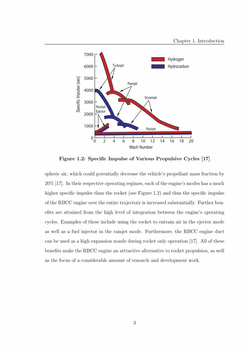
Figure 1.2: Specific Impulse of Various Propulsive Cycles [17]
spheric air, which could potentially decrease the vehicle’s propellant mass fraction by
20% [17]. In their respective operating regimes, each of the engine’s modes has a much
higher specific impulse than the rocket (see Figure 1.2) and thus the specific impulse
of the RBCC engine over the entire trajectory is increased substantially. Further ben-
efits are attained from the high level of integration between the engine’s operating
cycles. Examples of these include using the rocket to entrain air in the ejector mode
as well as a fuel injector in the ramjet mode. Furthermore, the RBCC engine duct
can be used as a high expansion nozzle during rocket only operation [17]. All of these
benefits make the RBCC engine an attractive alternative to rocket propulsion, as well
as the focus of a considerable amount of research and development work.
3
Chapter 1. Introduction
1.2 Literature Review
To date, this research has spawned numerous RBCC engine concepts all at different
stages of development. Most of these emerged from an industry-based NASA funded
study in the mid 1960’s, which evaluated 36 potential engine designs to replace the
multistage rocket propulsion system used in the space shuttle [26]. Twelve concepts,
including the RBCC engine were identified as the most promising and were thus
funded for further research [17]. The most promising ones were variants of an Ejector
Scramjet (ESJ) with different subsystems installed to further improve performance.
One of the configurations is Marquardt’s Supercharged Ejector Scramjet (SESJ) [25].
The SESJ was designed to be used for future high speed space transportation sys-
tems and has been studied by Marquardt both conceptually and experimentally. The
engine uses a dual concentric annular nozzle embedded inside an axisymmetric flow-
path. The engine also houses an integrated fan stage which boosts the performance of
the low-speed airbreathing modes (hence the term “supercharged”). Another relative
of the ESJ is Aerojet’s Strutjet engine [11]. This particular engine has a three-
dimensional asymmetric flowpath with embedded streamwise struts. The struts not
only enhance mixing and compression within the engine but are also used to efficiently
house various engine components such as the primary rockets and fuel injectors.
At low speeds (M < 1), the performance of the RBCC engine depends on the
operation of the rocket ejector, which tends to produce the lowest levels of thrust
augmentation as compared to the high speed modes. At these speeds, the perfor-
mance of the ejector depends on three fundamental processes, namely the entrain-
ment of atmospheric air, mixing of the two streams and finally the combustion of
the rocket/air mixture within the engine duct. The entrainment of atmospheric air,
for example, is required not only to increase the mass flow rate through the engine,
but also to supply the fresh oxygen required for combustion. The entrained air must
4
Chapter 1. Introduction
then fully mix with the rocket exhaust to achieve high compression as well as a uni-
form fuel/oxidizer distribution. Since longer ducts may be required to achieve a fully
mixed flow, poor mixing can increase engine weight, reduce ejector compression and
combustion efficiency thereby offsetting any performance gains.
The mixing kinetics inside an ejector can be studied in isolation by implementing
so called cold flow experiments, where the primary rocket stream is replaced with
either air or nitrogen at room temperature. This approach has the advantage of
decoupling the mixing from the combustion, in an experimental sense, but lacks the
realistic temperatures that are generally encountered in real ejectors. Despite this,
there have been many studies, with the earliest dating back to the mid 1950’s with
the experimental/theoretical work of Fabri & Paulon [30]. The purpose of their
experiments was to characterize the operation of an ejector over a wide range of
operating conditions. They were also among the first to identify the various operating
regimes of the ejector, such as the supersonic regime (sometimes called a “Fabri
Choke” [67]). In this regime, the high-pressure primary stream interacts with the
entrained air flow and creates an aerodynamic throat which can choke the air stream.
More recent experimental studies have been aimed at reducing ejector mixing
lengths through various means. For example, Kitamura et al. [44, 45] focused on the
geometry of the ejector, and studied the performance of various mixing tube cross-
sections. In their work, pressure recovery lengths were used to quantify the mixing
performance of axisymmetric, as well as straight and diverging rectangular geometries.
The studies showed that the pressure recovery lengths of axisymmetric ducts were
50% shorter than the rectangular ones, and that the divergent mixing tubes suffered
higher total pressure losses. Lineberry & Landrum [49], went a different route and
used a Strutjet-type experimental set-up to assess the use of multiple rocket nozzles
in an ejector. Their results showed that higher rocket chamber pressures tended to
increase the ejector mixing length, which was strongly dependent on the mass flow
5
Chapter 1. Introduction
rate of the primary stream.
To study ejectors under more realistic operating conditions, cold flow experiments
can be modified by heating the primary stream. This is done to experimentally
quantify the effects that high temperatures have on ejector performance. Although
basic thermodynamics can show that high temperatures increase impact losses in fully
mixed ejectors, its effects on the turbulent mixing process require detailed experimen-
tal studies. One such study was carried out by Quinn [61], who demonstrated that the
effect of high temperatures varied depending on the extent of mixing in the ejector.
His data showed that a hot primary stream has a slightly favourable effect in short,
partially mixed ejectors (L/D ≤ 6) due to the higher viscosity. In longer ejectors, on
the other hand, where the flows are fully mixed, higher temperatures were shown to
decrease air entrainment.
There have also been attempts to improve the mixing in the ejector by modifying
the primary flow nozzle. Several concepts have been suggested, such as the use of
so-called hypermixing nozzles [8] or forced mixer lobes [59]. Both methods derive
from the concept of inducing large scale axial vorticity within the ejector to aid
in mixing. This type of “convective” mixing is more efficient than shear mixing
according to Presz et. al. [59], and can result in nearly complete mixing. The use of
such mixing augmentation was originally intended to increase the thrust of ejectors
used on VSTOL aircraft, while forced mixer lobes have been used in gas turbine
engines. Subsonic studies were carried out by various researchers [8,31,60] to evaluate
different hypermixing nozzle arrangements. It was shown that the nozzles significantly
enhanced mixing of the two streams, and high levels of thrust augmentation (≈ 2)
can be achieved [60]. It was later shown by Tilllman et al. [66] that the same types of
mixer lobes used by Presz et al. [59] in their subsonic experiments, work equally well
for supersonic primary streams. In fact, his results showed that improved pumping
and near ideal mixing can be achieved without flow separation.
6
Chapter 1. Introduction
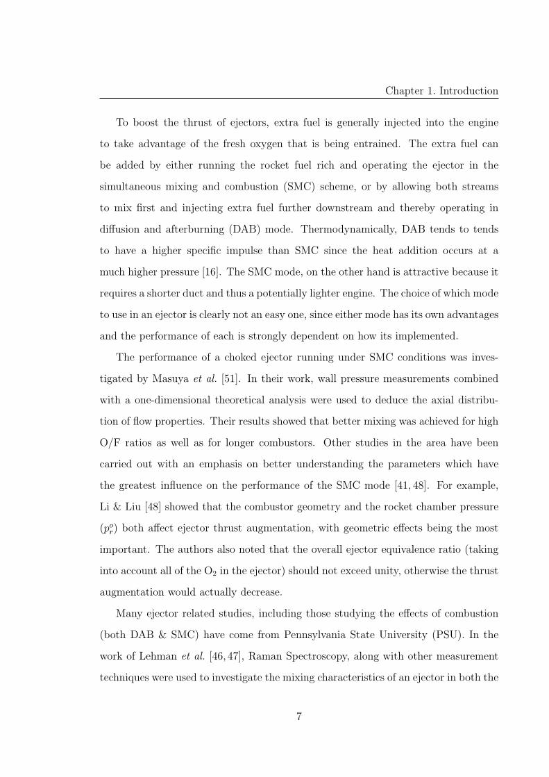
To boost the thrust of ejectors, extra fuel is generally injected into the engine
to take advantage of the fresh oxygen that is being entrained. The extra fuel can
be added by either running the rocket fuel rich and operating the ejector in the
simultaneous mixing and combustion (SMC) scheme, or by allowing both streams
to mix first and injecting extra fuel further downstream and thereby operating in
diffusion and afterburning (DAB) mode. Thermodynamically, DAB tends to tends
to have a higher specific impulse than SMC since the heat addition occurs at a
much higher pressure [16]. The SMC mode, on the other hand is attractive because it
requires a shorter duct and thus a potentially lighter engine. The choice of which mode
to use in an ejector is clearly not an easy one, since either mode has its own advantages
and the performance of each is strongly dependent on how its implemented.
The performance of a choked ejector running under SMC conditions was inves-
tigated by Masuya et al. [51]. In their work, wall pressure measurements combined
with a one-dimensional theoretical analysis were used to deduce the axial distribu-
tion of flow properties. Their results showed that better mixing was achieved for high
O/F ratios as well as for longer combustors. Other studies in the area have been
carried out with an emphasis on better understanding the parameters which have
the greatest influence on the performance of the SMC mode [41, 48]. For example,
Li & Liu [48] showed that the combustor geometry and the rocket chamber pressure
(por) both affect ejector thrust augmentation, with geometric effects being the most
important. The authors also noted that the overall ejector equivalence ratio (taking
into account all of the O2 in the ejector) should not exceed unity, otherwise the thrust
augmentation would actually decrease.
Many ejector related studies, including those studying the effects of combustion
(both DAB & SMC) have come from Pennsylvania State University (PSU). In the
work of Lehman et al. [46, 47], Raman Spectroscopy, along with other measurement
techniques were used to investigate the mixing characteristics of an ejector in both the
7
Chapter 1. Introduction
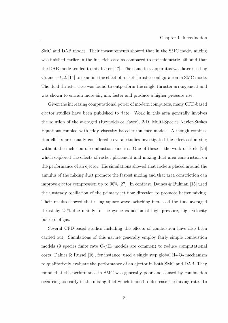
SMC and DAB modes. Their measurements showed that in the SMC mode, mixing
was finished earlier in the fuel rich case as compared to stoichiometric [46] and that
the DAB mode tended to mix faster [47]. The same test apparatus was later used by
Cramer et al. [14] to examine the effect of rocket thruster configuration in SMC mode.
The dual thruster case was found to outperform the single thruster arrangement and
was shown to entrain more air, mix faster and produce a higher pressure rise.
Given the increasing computational power of modern computers, many CFD-based
ejector studies have been published to date. Work in this area generally involves
the solution of the averaged (Reynolds or Favre), 2-D, Multi-Species Navier-Stokes
Equations coupled with eddy viscosity-based turbulence models. Although combus-
tion effects are usually considered, several studies investigated the effects of mixing
without the inclusion of combustion kinetics. One of these is the work of Etele [26]
which explored the effects of rocket placement and mixing duct area constriction on
the performance of an ejector. His simulations showed that rockets placed around the
annulus of the mixing duct promote the fastest mixing and that area constriction can
improve ejector compression up to 30% [27]. In contrast, Daines & Bulman [15] used
the unsteady oscillation of the primary jet flow direction to promote better mixing.
Their results showed that using square wave switching increased the time-averaged
thrust by 24% due mainly to the cyclic expulsion of high pressure, high velocity
pockets of gas.
Several CFD-based studies including the effects of combustion have also been
carried out. Simulations of this nature generally employ fairly simple combustion
models (9 species finite rate O2/H2 models are common) to reduce computational
costs. Daines & Russel [16], for instance, used a single step global H2-O2 mechanism
to qualitatively evaluate the performance of an ejector in both SMC and DAB. They
found that the performance in SMC was generally poor and caused by combustion
occurring too early in the mixing duct which tended to decrease the mixing rate. To
8
Chapter 1. Introduction
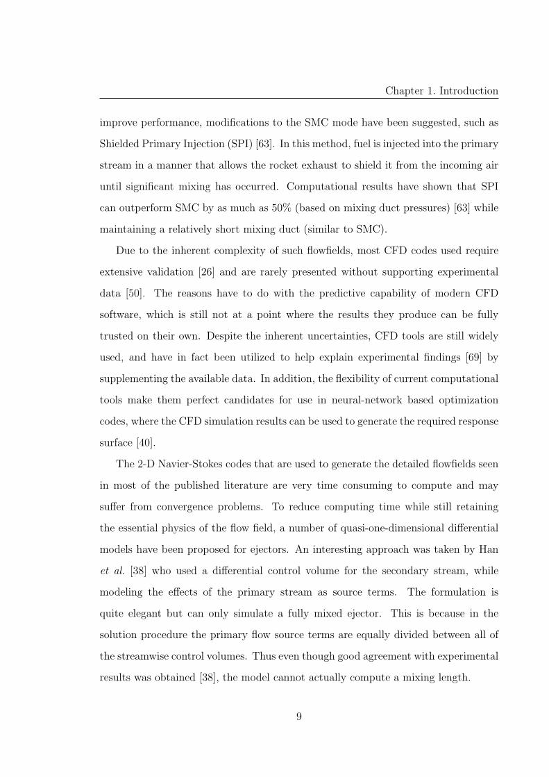
improve performance, modifications to the SMC mode have been suggested, such as
Shielded Primary Injection (SPI) [63]. In this method, fuel is injected into the primary
stream in a manner that allows the rocket exhaust to shield it from the incoming air
until significant mixing has occurred. Computational results have shown that SPI
can outperform SMC by as much as 50% (based on mixing duct pressures) [63] while
maintaining a relatively short mixing duct (similar to SMC).
Due to the inherent complexity of such flowfields, most CFD codes used require
extensive validation [26] and are rarely presented without supporting experimental
data [50]. The reasons have to do with the predictive capability of modern CFD
software, which is still not at a point where the results they produce can be fully
trusted on their own. Despite the inherent uncertainties, CFD tools are still widely
used, and have in fact been utilized to help explain experimental findings [69] by
supplementing the available data. In addition, the flexibility of current computational
tools make them perfect candidates for use in neural-network based optimization
codes, where the CFD simulation results can be used to generate the required response
surface [40].
The 2-D Navier-Stokes codes that are used to generate the detailed flowfields seen
in most of the published literature are very time consuming to compute and may
suffer from convergence problems. To reduce computing time while still retaining
the essential physics of the flow field, a number of quasi-one-dimensional differential
models have been proposed for ejectors. An interesting approach was taken by Han
et al. [38] who used a differential control volume for the secondary stream, while
modeling the effects of the primary stream as source terms. The formulation is
quite elegant but can only simulate a fully mixed ejector. This is because in the
solution procedure the primary flow source terms are equally divided between all of
the streamwise control volumes. Thus even though good agreement with experimental
results was obtained [38], the model cannot actually compute a mixing length.
9

Chapter 1. Introduction
Another such model has been proposed by Yungster & Trefny [70] specifically for
NASA’s Independent Ramjet Stream (IRS) Cycle. In the IRS cycle, the secondary
(air) stream is pre-fueled far upstream of the rocket resulting in a pre-mixed fuel/air
mixture. The rocket is then used only as a source of ignition for the secondary stream,
and thus mixing between the flows is not required for thrust augmentation. This par-
ticular cycle has actually been the subject of several computational studies [9,65], such
as tailoring the fuel injection scheme to alter the location of the thermal throat [65],
(which was shown to be feasible for a standard ejector [31]). The differential model
of Yungster & Trefny [70] uses separate control volumes for the primary and sec-
ondary streams, while neglecting the shear layer since no mixing is assumed to occur.
The streamline which divides the two control volumes is calculated with an empirical
pressure-based equation (i.e., Astream ∝ (pp−ps)). In addition, chemical reactions are
modeled using a heat release function specified between two assumed points which
signify the start and end of the heat release. This model agreed very well with ana-
lytical benchmark tests [70] carried out by the authors (i.e., Rayleigh flow), but it has
not yet been compared to Navier-Stokes based simulations or experimental results.
Analyses of a more fundamental nature, in the form of the basic integral conser-
vation laws have also been applied to ejectors. The goal in this case is to establish
fundamental operating trends as well as to identify the dimensionless parameters
which govern ejector performance (α, ζ, θ, etc.). Such treatments generally employ
the Inviscid, quasi-one-dimensional conservation laws (mass, momentum, energy) ap-
plied to a straight wall mixing duct, subject to specific assumptions about how the
two streams initially interact. The majority of the theoretical treatments on ejec-
tors further assume that the two streams fully mix, which essentially represents the
ideal case, or the maximum performance that a given ejector configuration can ob-
tain. Analysis under non-ideal, partially-mixed conditions are limited to the work of
Papamoschou [57]. In his analysis, conservation laws are applied separately to each
10
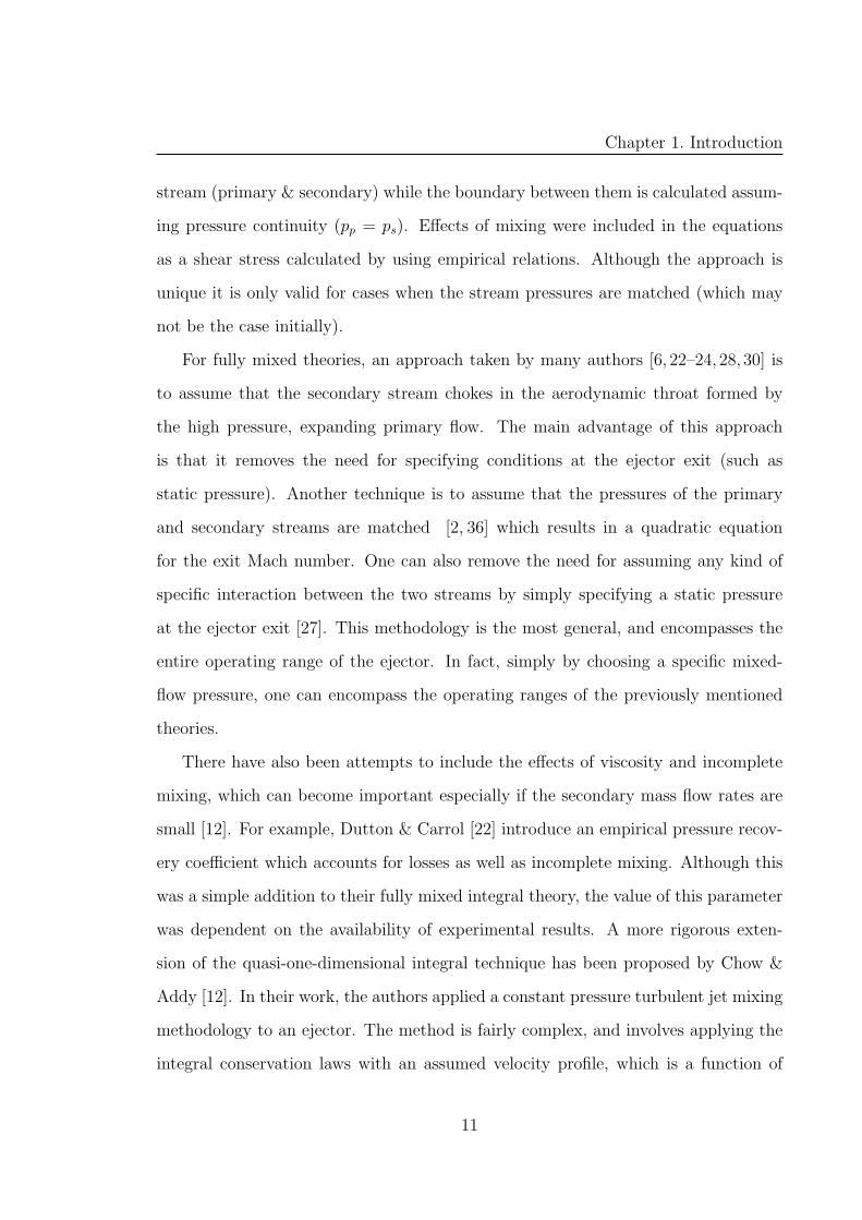
Chapter 1. Introduction
stream (primary & secondary) while the boundary between them is calculated assum-
ing pressure continuity (pp = ps). Effects of mixing were included in the equations
as a shear stress calculated by using empirical relations. Although the approach is
unique it is only valid for cases when the stream pressures are matched (which may
not be the case initially).
For fully mixed theories, an approach taken by many authors [6, 22–24, 28, 30] is
to assume that the secondary stream chokes in the aerodynamic throat formed by
the high pressure, expanding primary flow. The main advantage of this approach
is that it removes the need for specifying conditions at the ejector exit (such as
static pressure). Another technique is to assume that the pressures of the primary
and secondary streams are matched [2, 36] which results in a quadratic equation
for the exit Mach number. One can also remove the need for assuming any kind of
specific interaction between the two streams by simply specifying a static pressure
at the ejector exit [27]. This methodology is the most general, and encompasses the
entire operating range of the ejector. In fact, simply by choosing a specific mixed-
flow pressure, one can encompass the operating ranges of the previously mentioned
theories.
There have also been attempts to include the effects of viscosity and incomplete
mixing, which can become important especially if the secondary mass flow rates are
small [12]. For example, Dutton & Carrol [22] introduce an empirical pressure recov-
ery coefficient which accounts for losses as well as incomplete mixing. Although this
was a simple addition to their fully mixed integral theory, the value of this parameter
was dependent on the availability of experimental results. A more rigorous exten-
sion of the quasi-one-dimensional integral technique has been proposed by Chow &
Addy [12]. In their work, the authors applied a constant pressure turbulent jet mixing
methodology to an ejector. The method is fairly complex, and involves applying the
integral conservation laws with an assumed velocity profile, which is a function of
11
Chapter 1. Introduction
various empirical parameters related to the mixing of the two jets.
The effects of combustion have also been incorporated in several of the integral-
based theories in open literature. In a paper by Han et al. [36], combustion kinetics
were treated very simply by adding a source term to the energy equation. A similar
approach was adopted by Dobrowolski [20], who used the analysis to theoretically
establish that DAB operation is more efficient than SMC. What sets his work apart
from the rest, is that his analysis included the effects of a variable area mixing duct
by integrating the Crocco Pressure-Area Relation [20] and using it in the momentum
equation. The relation has a power law form, and was originally used for single stream
devices, such as ramjets. A more detailed treatment of the mixing and combustion
processes in an ejector was presented by Peters et al. [58]. Their work was more
focused on modeling the mixing process using a modification of the model of Chow &
Addy [12]. However, in contrast to the previously mentioned approaches, the authors
invoked chemical equilibrium relations to include the effects of combustion.
1.3 Objectives
The goal of the current work will be to present an analysis methodology for an
ejector that is simple enough to rapidly examine a large number of configurations
and accurate enough for use during the initial design stage. The theory will assume
complete mixing and will therefore be used to provide idealized performance estimates
for the subsonic flight speed range. What sets the present work apart from the rest
is its ability to analyze ejector configurations not covered by the approaches available
in open literature and to do so in a more complete manner, while maintaining an
equation set which can be solved very quickly. Specifically, the theory that will be
presented will focus on an annular rocket configuration since it has been shown to
promote better mixing [29] and is thus more likely to be used in an ejector design.
12

Chapter 1. Introduction
The performance of an ejector can be improved further by constricting its mixing
duct which has been shown to improve the compression ratio [27]. For this reason
the formulation will also enable analysis of converging mixing ducts and although one
such theory was found in literature it was only applicable for ejectors with a central
rocket configuration [20]. The combustion in the ejector under SMC conditions will
be treated in detail by using an equilibrium calculation which can account for a large
number of species. Finally, a method will be provided to estimate a mixing length as
well as any performance losses due to incomplete mixing by modifying the equations
for the fully mixed-case.
13
Chapter 2
Non-Reacting Ejector Theory
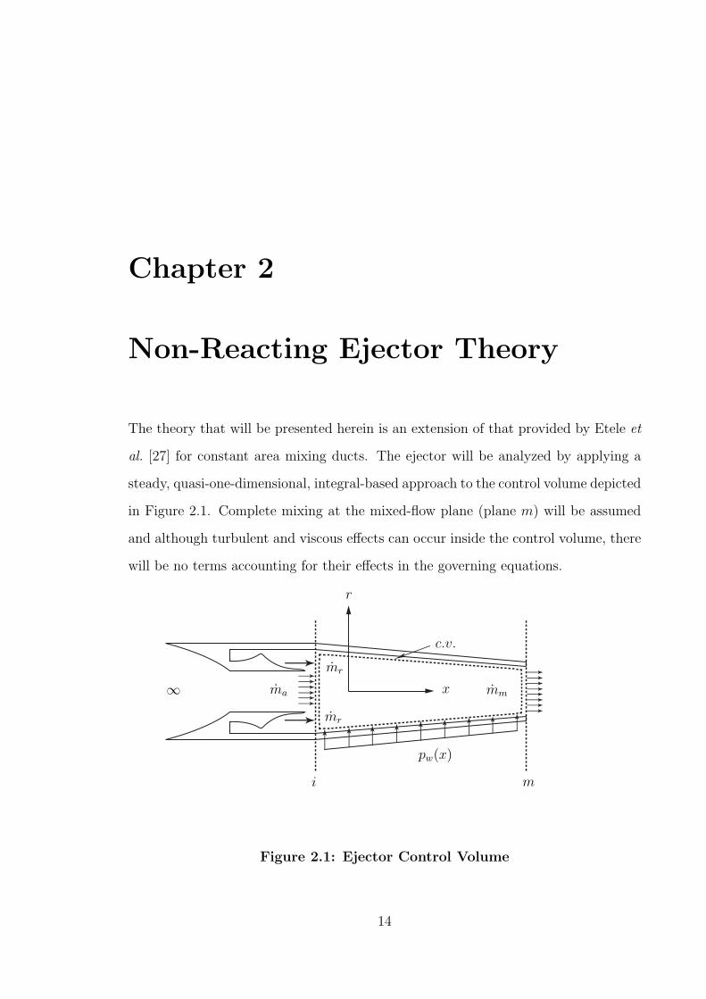
The theory that will be presented herein is an extension of that provided by Etele et
al. [27] for constant area mixing ducts. The ejector will be analyzed by applying a
steady, quasi-one-dimensional, integral-based approach to the control volume depicted
in Figure 2.1. Complete mixing at the mixed-flow plane (plane m) will be assumed
and although turbulent and viscous effects can occur inside the control volume, there
will be no terms accounting for their effects in the governing equations.
mr
mr
ma mm∞
i m
c.v.
pw(x)
r
x
Figure 2.1: Ejector Control Volume
14
Chapter 2. Non-Reacting Ejector Theory
Considering the mass flow rates shown in Figure 2.1 the conservation of mass can
be expressed as,
ma + mr = mm (2.1)
The mass flow rates in Eq. (2.1) can be more conveniently written in terms of total
conditions, to give,
m
A= po
√γ
RT o
M
(1 + γ−1
2M2
)1/2
(1 + γ−1
2M2
) γγ−1
which then simplifies to
m
A=( po
√RT o
)µ (2.2)
with the functional µ defined as,
µ(γ,M) =√γM
(1 +
γ − 1
2M2
)−(γ+1)2(γ−1)
(2.3)
Substituting Eq. (2.2) into Eq. (2.1) and re-arranging gives the first equation for the
mixed-flow Mach number, Mm,
mr
pmAm
√RmT o
m
γm
(α+ 1) = Mm
(1 +
γm − 1
2M2
m
)1/2
(2.4)
where α is the entrainment ratio and is defined as,
α = ma/mr (2.5)
Neglecting viscous forces, the momentum equation for the ejector control volume
can be written as follows:
(maua + paAa) + (mrur + prAr) − (mmum + pmAm) −∫∫ L
0
pw(x) · d~Sx = 0 (2.6)
15

Chapter 2. Non-Reacting Ejector Theory
The air and rocket momentum terms can be re-expressed using the ideal-gas law and
the definition of the speed of sound,
(mu+ pA) = ma(M +
p
ρua
)A = ma
(M +
1
γM
)(2.7)
The speed of sound can then be related to sonic conditions in the following manner:
a
a∗=
√T
T ∗
=
√1 + γ−1
2
1 + γ−1
2M2
=1√
2
γ+1+(
γ−1
γ+1
)M2
(2.8)
Using Eq. (2.8) to replace the speed of sound in Eq. (2.7) yields,
ma(M +
1
γM
)= ma∗χ (2.9)
where χ is defined as,
χ(γ,M) =
[M + 1
γM√2
γ+1+(
γ−1
γ+1
)M2
](2.10)
Substituting equations (2.7) & (2.9) into Eq. (2.6) and manipulating the exit mo-
mentum flux so as to explicitly maintain the mixed-flow pressure, one obtains,
maa∗χa + mra
∗
rχr − pmAm
(γM2
m + 1)−∫∫ L
0
pw(x) · d~Sx = 0 (2.11)
At sonic conditions, the speed of sound can be expressed as,
a∗2 = 2Cpγ − 1
γ + 1T o (2.12)
16
Chapter 2. Non-Reacting Ejector Theory
thereby allowing one to write the ratio of the air/rocket sonic sound speeds as,
a∗aa∗r
=√θΓ (2.13)
where θ and Γ have the following definitions:
θ =Cp,aT
oa
Cp,rT or
(2.14)
Γ =
√(γa − 1)(γr + 1)
(γa + 1)(γr − 1)(2.15)
One can then invoke the definition of α along with Eq. (2.13) to simplify Eq. (2.11)
and yield a second equation for Mm,
M2m =
1
γm
[mra
∗
r
pmAm
(α√θΓχa + χr) − Fp,x − 1
](2.16)
where the term Fp,x defines the dimensionless wall pressure force,
Fp,x =1
pmAm
∫∫ L
0
pw(x) · d~Sx (2.17)
At this point it is convenient to relate the entrainment ratio to other ejector
variables by substituting Eq. (2.2) into (2.5) to give,
α =1
ζ
(1 − σ
σ
) 1√θ
[γa(γr − 1)
γr(γa − 1)
]1/2µa
µr
with the following additional definitions:
σ =Ar
Ai
(2.18)
17
Chapter 2. Non-Reacting Ejector Theory
ζ =po
r
poa
(2.19)
Since only the µ functionals depend on the solution variables, α can be more conve-
niently re-expressed as,
α = ψµa
µr
(2.20)
where
ψ =1
ζ
(1 − σ
σ
) 1√θ
(γa(γr − 1)
γr(γa − 1)
)1/2
(2.21)
With no heat losses or chemical reactions, the conservation of energy for the ejector
simply becomes a conservation of total enthalpy,
maCp,aToa + mrCp,rT
or = mmCp,mT
om (2.22)
Invoking mass conservation and re-arranging gives,
mr
(ma
mr
Cp,aToa
Cp,rT or
+ 1
)= mr
(ma
mr
+ 1
)Cp,mT
om
Cp,rT or
The definitions of α and θ can then be used to simplify the energy equation and give
the following result,
T om =
Cp,r
Cp,m
(αθ + 1
α+ 1
)T o
r (2.23)
Assuming complete mixing at the exit, mass averaging can be used to relate the
gas properties to the entrainment ratio,
Wm =1
α+ 1(αWa +Wr) (2.24)
γm =1
α+ 1(αγa + γr) (2.25)
Ideal gas relations can then be used to solve for the gas constant and the specific heat
18
Chapter 2. Non-Reacting Ejector Theory
of the mixture,
Rm =Ru
Wm
(2.26)
Cp,m =γmRm
γm − 1(2.27)
Equations (2.4), (2.16) & (2.23) represent a system of three equations in the five
unknowns, namely µa, χa,Mm, Tom and Fp,x. However, from equations (2.10) & (2.3) it
is clear that both χa and µa depend on the air inflow Mach number, Ma. Thus if one
can relate Fp,x to other ejector variables, the system will only have three unknowns
(Ma,Mm,T om) and can therefore be solved. To implement the solution one needs to
know the total inlet conditions (T oa , T
or , p
or, p
oa ), the ejector geometry (σ,A(x)), the
rocket exhaust Mach number Mr, the inlet gas composition (Ra, Rr, γa, γr) and the
exit pressure pm.
2.1 Wall Pressure Distribution
To relate the dimensionless wall pressure force to other ejector variables, a wall pres-
sure distribution is required. Since in general, such information will not be known a
priori, one has to assume a functional form for pw(x). One can consider two repre-
sentative cases. The first is the simplest, the case where no additional information
about the ejector flowfield is known. This is a linear pressure distribution given by
Eq. (2.28) which depends only on the pressure at each end of the ejector. Since the
present theory will focus on a configuration with an annular rocket, then the pressure
at the ejector inlet will simply be pr while the pressure at the outlet is the mixed-flow
pressure pm.
pw(x) = pr + (pm − pr)x
L(2.28)
19
Chapter 2. Non-Reacting Ejector Theory
The second is slightly more complex and is designed to qualitatively model the
expansion-recompression process that occurs inside the ejector. This pressure dis-
tribution is given by Eq. (2.29) and depends on the minimum pressure to which the
rocket plume expands in addition to the pressure boundary conditions.
pw(x) = pmin + c1
[c2 − (
x
L− 1)2
]2(2.29)
The constants c1 and c2 can be found by applying the pressure boundary conditions
(i.e., pw(0) = pr, pw(L) = pm) to give,
c2 =(1 +
√β)−1
(2.30)
c1 =pm − pmin
c22(2.31)
where
β =pr − pmin
pm − pmin
(2.32)
The parameter pmin represents the minimum pressure to which the rocket exhaust
expands and requires additional equations for its quantification.
2.2 Solution for Minimum Rocket Pressure
It is clear at this point that if one wishes to use Eq. (2.29) a way of solving for
the parameter pmin is required. Two different methods are presented to solve for the
minimum rocket pressure, the first is a Control Volume calculation, while the second
one makes use of a Riemann solver. Both methods assume that the air and rocket
streams are isentropic and that no mixing takes place before the expansion point.
20
Chapter 2. Non-Reacting Ejector Theory
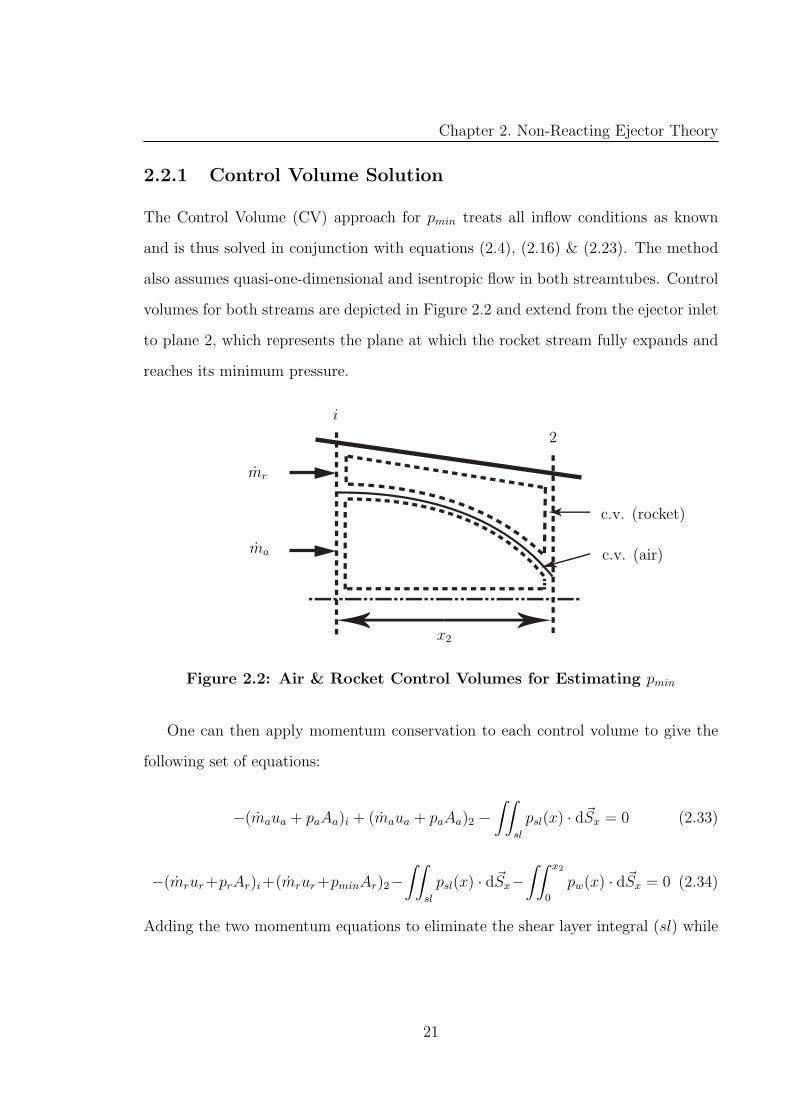
2.2.1 Control Volume Solution
The Control Volume (CV) approach for pmin treats all inflow conditions as known
and is thus solved in conjunction with equations (2.4), (2.16) & (2.23). The method
also assumes quasi-one-dimensional and isentropic flow in both streamtubes. Control
volumes for both streams are depicted in Figure 2.2 and extend from the ejector inlet
to plane 2, which represents the plane at which the rocket stream fully expands and
reaches its minimum pressure.
ma
mr
c.v. (air)
i
2
c.v. (rocket)
x2
Figure 2.2: Air & Rocket Control Volumes for Estimating pmin
One can then apply momentum conservation to each control volume to give the
following set of equations:
−(maua + paAa)i + (maua + paAa)2 −∫∫
sl
psl(x) · d~Sx = 0 (2.33)
−(mrur+prAr)i+(mrur+pminAr)2−∫∫
sl
psl(x) · d~Sx−∫∫ x2
0
pw(x) · d~Sx = 0 (2.34)
Adding the two momentum equations to eliminate the shear layer integral (sl) while
21
Chapter 2. Non-Reacting Ejector Theory
using equations (2.7) & (2.9) to simplify the momentum fluxes yields,
ma(χa,2a∗
a,2 − χa,ia∗
a,i) + mr(χr,2a∗
r,2 − χr,ia∗
r,i) −∫∫ x2
0
pw(x) · d~Sx = 0 (2.35)
Since both streams do not mix and are adiabatic, then by Eq. (2.12):
a∗a,i = a∗a,2 = a∗a
a∗r,i = a∗r,2 = a∗r
which allows the definitions of α, θ & Γ to be used to simplify Eq. (2.35),
(χr,i − χr,2) + α√θΓ(χa,i − χa,2) − Fp,x2 = 0 (2.36)
where
Fp,x2 =1
mra∗r
∫∫ x2
0
pw(x) · d~Sx (2.37)
The term Fp,x2 has the same form as Eq. (2.17) but is integrated only up to the point
where the rocket stream reaches its minimum pressure. The axial location of this
point can be obtained directly from Eq. (2.29) by minimizing the expression to give,
x2
L= 1 −√
c2 (2.38)
Equations (2.29) & (2.38) can be substituted into the expression for Fp,x2 and inte-
grated to obtain a closed-form expression (Eq. (2.85)) in terms of the constants c1
& c2. Since both of these constants are functions of pmin (see Eq’s (2.31), (2.30),
(2.32)), the dimensionless pressure integral (Fp,x2) becomes a function of the solution
variable, pmin.
22
Chapter 2. Non-Reacting Ejector Theory
Next, the conservation of mass is applied to the air control volume in conjunction
with Eq. (2.2) to obtain,
Aa,i
poa,i√RaT o
a,i
µa,i = Aa,2
poa,2√RaT o
a,2
µa,2 (2.39)
Since the flow is both isentropic and adiabatic, the above equation reduces to,
Aa,iµa,i = Aa,2µa,2 (2.40)
Applying the same approach to the rocket stream gives,
Ar,iµr,i = Ar,2µr,2 (2.41)
Given the fact that the flow areas at station 2 are constrained,
Ar,2 + Aa,2 = A(x2) (2.42)
allows equations (2.40), (2.41) and (2.42) to be combined into an expression in terms
of the air/rocket Mach numbers only,
Aa,iµa,i
µa,2
+ Ar,iµr,i
µr,2
= A(x2) (2.43)
Since both streams were assumed isentropic, pmin can be related to Mr,2 with the
isentropic expression for total pressure which can be written as,
pmin = por
(1 +
γr − 1
2M2
r,2
) −γrγr−1
(2.44)
The derivation thus yields two equations, (2.36) & (2.43) in the unknowns µa,2, χa,2,
µr,2, χr,2 and pmin. If one invokes the definitions of µ and χ as well as Eq. (2.44), the
23
Chapter 2. Non-Reacting Ejector Theory
unknowns are reduced to the air and rocket Mach numbers, Ma,2 and Mr,2. It should
be noted that since the solution for pmin requires knowledge of the ejector inflow
conditions (Ma), it must be repeated at each iteration of the solution of equations
(2.4), (2.16) & (2.23).
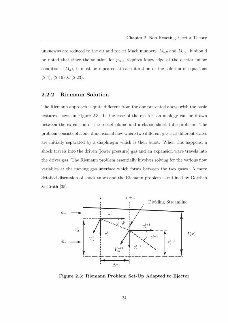
2.2.2 Riemann Solution
The Riemann approach is quite different from the one presented above with the basic
features shown in Figure 2.3. In the case of the ejector, an analogy can be drawn
between the expansion of the rocket plume and a classic shock tube problem. The
problem consists of a one-dimensional flow where two different gases at different states
are initially separated by a diaphragm which is then burst. When this happens, a
shock travels into the driven (lower pressure) gas and an expansion wave travels into
the driver gas. The Riemann problem essentially involves solving for the various flow
variables at the moving gas interface which forms between the two gases. A more
detailed discussion of shock tubes and the Riemann problem is outlined by Gottlieb
& Groth [35].
V i+1cs
i i+ 1
mr
ma
A(x)ria
ri+1a
∆x
Dividing Streamline
vi+1r
ui+1r
uir
V ics
vir
δi
δi+1
Figure 2.3: Riemann Problem Set-Up Adapted to Ejector
24
Chapter 2. Non-Reacting Ejector Theory
Referring to Fig. 2.3, the method is set up such that the radial motion of the
rocket plume expanding against the air stream at some location x is treated as a
shock tube. For the case when the rocket pressure exceeds the static pressure of the
air, the rocket plume becomes the driver gas. Since the streams are assumed not to
mix, one can define a contact surface, or more generally a dividing streamline which
separates the two streams. In the present case, a Riemann solver is used to solve for
the velocity of the contact surface which along with the streamwise velocity can be
used to trace out the dividing streamline. The streamline would then define the area
distribution of the streamtubes which surround each stream at which point isentropic
relations can be used to find the remaining flow variables. The present formulation
uses a Riemann solver proposed by Gottlieb & Groth [35] to solve for Vcs.
First, from the Mach numbers of the rocket and air streams the sonic reference
areas can be found using the Area-Mach Number Relation [3].
f
(A
A∗
)=
1
M2
(2
γ + 1+γ − 1
γ + 1M2
) γ+1γ−1
=
(A
A∗
)2
(2.45)
Next the Riemann solver is applied to find the velocity of the contact surface at node
i.
V ics = f(pi
r, pia, ρ
ir, ρ
ia, Rr, Ra, γr, γa) (2.46)
To define the streamline at the next node, the radial velocity component at node i+1
is required which can be written as,
vi+1r = vi
r + ∆vr (2.47)
Referring to the velocity polygon shown in Fig. 2.4 one can express ∆vr as,
∆vr = V icscos(δi) =
V icsu
ir√
[uir]
2 + [vir]
2(2.48)
25
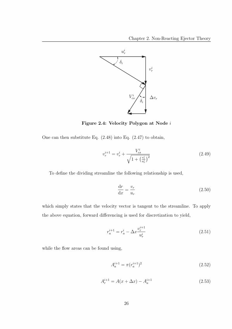
Chapter 2. Non-Reacting Ejector Theory
uir
vir
V ics
δi
δi
∆vr
Figure 2.4: Velocity Polygon at Node i
One can then substitute Eq. (2.48) into Eq. (2.47) to obtain,
vi+1r = vi
r +V i
cs√1 +
(vi
r
uir
)2 (2.49)
To define the dividing streamline the following relationship is used,
dr
dx=vr
ur
(2.50)
which simply states that the velocity vector is tangent to the streamline. To apply
the above equation, forward differencing is used for discretization to yield,
ri+1a = ri
a − ∆xvi+1
r
uir
(2.51)
while the flow areas can be found using,
Ai+1a = π(ri+1
a )2 (2.52)
Ai+1r = A(x+ ∆x) − Ai+1
a (2.53)
26
Chapter 2. Non-Reacting Ejector Theory
With the flow areas known, the Area-Mach Number Relation can be used to solve for
the Mach number,
M i+1
j = f(Ai+1
j
A∗
j
)j = a, r (2.54)
after which isentropic relations along with the ideal gas law are used to solve for the
state of each stream at i+ 1,
T i+1
j = T oj
[1 +
γj − 1
2(M i+1
j )2
]−1
j = a, r (2.55)
pi+1
j = poj
[1 +
γj − 1
2(M i+1
j )2
] −γjγj−1
j = a, r (2.56)
ρi+1
j =pi+1
j
RjTi+1
j
j = a, r (2.57)
Lastly, mass conservation can be used to solve for the axial velocity,
ui+1
j =mj
ρi+1
j Ai+1
j
j = a, r (2.58)
The procedure is then marched in the x-direction until vr ≤ 0 (the expansion
stops). One thing to note regarding the above procedure, is that the air stream can
choke while vr > 0. This type of situation would not happen in reality, since the
mass flow rate of the air at the inlet would adjust to accommodate a smaller A∗
a.
However, because pmin is solved at each iteration of the ejector solution, equations
(2.4), (2.16) & (2.23) govern the mass flow rate of the air, and not the Riemann
solver. Essentially, the type of feedback required to allow the air flow to adjust is
not possible to implement in the present formulation. Thus to be able to solve for
pmin when the air flow chokes, a slight modification to the solution process is made.
If critical conditions are encountered in the air stream during a given run while the
streamline is still expanding, the Riemann procedure is stopped. At the point where
the solver stops, it is then assumed that Aa = A∗
a. This fixes the area of the rocket
27
Chapter 2. Non-Reacting Ejector Theory
stream (by Eq. (2.42)), and allows one to use Eq. (2.45) to find the Mach number at
that station, from which pmin can be found using Eq. (2.56).
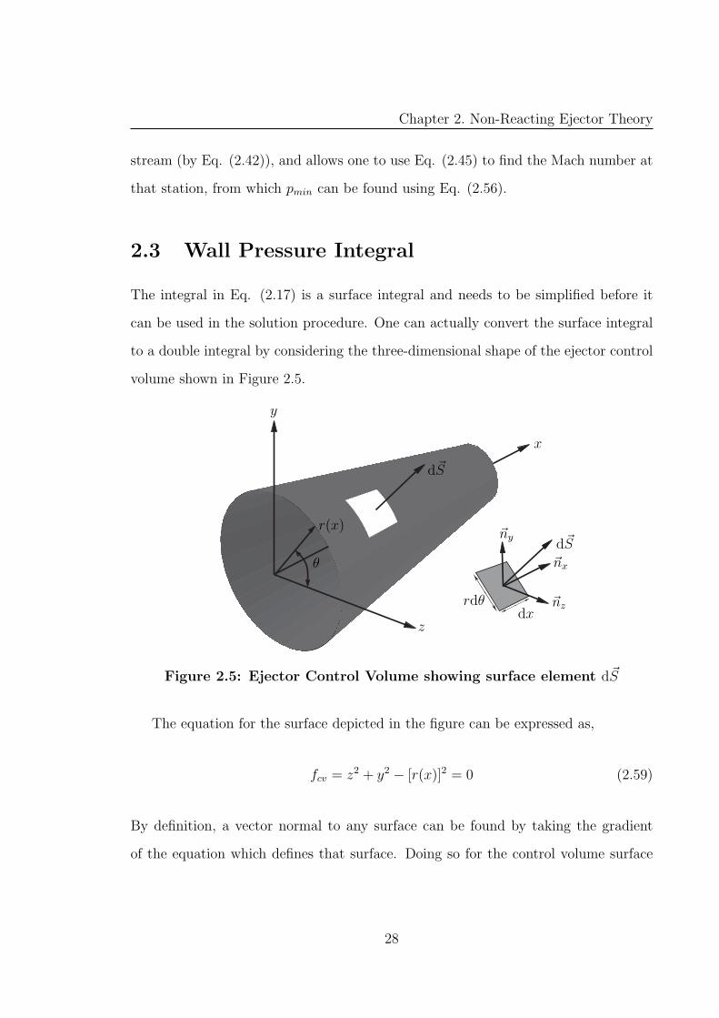
2.3 Wall Pressure Integral
The integral in Eq. (2.17) is a surface integral and needs to be simplified before it
can be used in the solution procedure. One can actually convert the surface integral
to a double integral by considering the three-dimensional shape of the ejector control
volume shown in Figure 2.5.
~nx
~ny
~nz
d~S
d~S
dxrdθ
θ
r(x)
x
y
z
Figure 2.5: Ejector Control Volume showing surface element d~S
The equation for the surface depicted in the figure can be expressed as,
fcv = z2 + y2 − [r(x)]2 = 0 (2.59)
By definition, a vector normal to any surface can be found by taking the gradient
of the equation which defines that surface. Doing so for the control volume surface
28
Chapter 2. Non-Reacting Ejector Theory
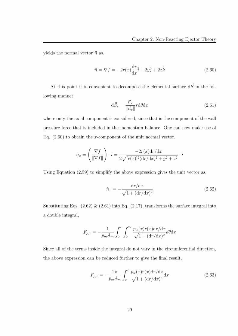
yields the normal vector ~n as,
~n = ∇f = −2r(x)dr
dxi+ 2yj + 2zk (2.60)
At this point it is convenient to decompose the elemental surface d~S in the fol-
lowing manner:
d~Sx =~nx
‖~nx‖rdθdx (2.61)
where only the axial component is considered, since that is the component of the wall
pressure force that is included in the momentum balance. One can now make use of
Eq. (2.60) to obtain the x-component of the unit normal vector,
nx =
(∇f‖∇f‖
)· i =
−2r(x)dr/dx
2√
[r(x)]2(dr/dx)2 + y2 + z2· i
Using Equation (2.59) to simplify the above expression gives the unit vector as,
nx = − dr/dx√1 + (dr/dx)2
(2.62)
Substituting Eqs. (2.62) & (2.61) into Eq. (2.17), transforms the surface integral into
a double integral,
Fp,x = − 1
pmAm
∫ L
0
∫ 2π
0
pw(x)r(x)dr/dx√1 + (dr/dx)2
dθdx
Since all of the terms inside the integral do not vary in the circumferential direction,
the above expression can be reduced further to give the final result,
Fp,x = − 2π
pmAm
∫ L
0
pw(x)r(x)dr/dx√1 + (dr/dx)2
dx (2.63)
29
Chapter 2. Non-Reacting Ejector Theory
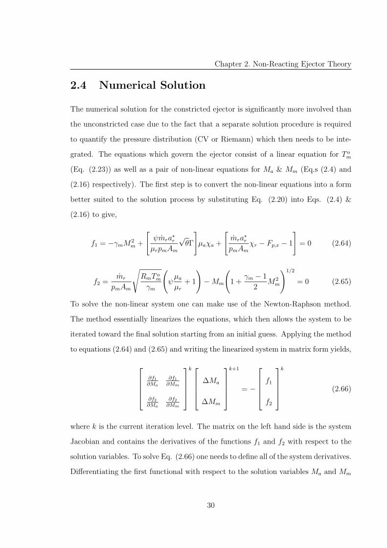
2.4 Numerical Solution
The numerical solution for the constricted ejector is significantly more involved than
the unconstricted case due to the fact that a separate solution procedure is required
to quantify the pressure distribution (CV or Riemann) which then needs to be inte-
grated. The equations which govern the ejector consist of a linear equation for T om
(Eq. (2.23)) as well as a pair of non-linear equations for Ma & Mm (Eq.s (2.4) and
(2.16) respectively). The first step is to convert the non-linear equations into a form
better suited to the solution process by substituting Eq. (2.20) into Eqs. (2.4) &
(2.16) to give,
f1 = −γmM2m +
[ψmra
∗
r
µrpmAm
√θΓ
]µaχa +
[mra
∗
r
pmAm
χr − Fp,x − 1
]= 0 (2.64)
f2 =mr
pmAm
√RmT o
m
γm
(ψµa
µr
+ 1
)−Mm
(1 +
γm − 1
2M2
m
)1/2
= 0 (2.65)
To solve the non-linear system one can make use of the Newton-Raphson method.
The method essentially linearizes the equations, which then allows the system to be
iterated toward the final solution starting from an initial guess. Applying the method
to equations (2.64) and (2.65) and writing the linearized system in matrix form yields,
∂f1
∂Ma
∂f1
∂Mm
∂f2
∂Ma
∂f2
∂Mm
k
∆Ma
∆Mm
k+1
= −
f1
f2
k
(2.66)
where k is the current iteration level. The matrix on the left hand side is the system
Jacobian and contains the derivatives of the functions f1 and f2 with respect to the
solution variables. To solve Eq. (2.66) one needs to define all of the system derivatives.
Differentiating the first functional with respect to the solution variables Ma and Mm
30
Chapter 2. Non-Reacting Ejector Theory
gives,
∂f1
∂Ma
=ψ√θΓmra
∗
r
µrpmAm
[µa
∂χa
∂Ma
+ χa∂µa
∂Ma
](2.67)
∂f1
∂Mm
= −2γmMm (2.68)
In a similar manner one can also obtain derivatives of the second functional to yield,
∂f2
∂Mm
= −(
1 +γm − 1
2M2
m
)1/2[(γm − 1)M2
m
2(1 + γm−1
2M2
m)+ 1
](2.69)
Keeping in mind that T om depends on Ma (through α) the derivative of Eq. (2.65)
with respect to Ma can be obtained as,
∂f2
∂Ma
=mr
pmAm
√RmT o
m
γm
[ψ
µr
∂µa
∂Ma
+(α+ 1)
2T om
∂T om
∂Ma
](2.70)
while the derivative of T om can be acquired from the energy equation, giving,
∂T om
∂Ma
=Cp,r
Cp,m
T or
∂µa
∂Ma
[(θ − 1)
(α+ 1)2
]ψ
µr
(2.71)
Lastly, the derivatives of the µ and χ functionals are required since they appear
several times. To obtain these one can simply differentiate Eqs. (2.3) and (2.10) to
give the following relations:
∂χ
∂M=
(2
γ + 1+γ − 1
γ + 1M2
)−1/2[(
1 − 1
γM2
)
−(M2 +
1
γ
)(γ − 1
γ + 1
)(2
γ + 1+γ − 1
γ + 1M2
)3](2.72)
∂µ
∂M=
√γ
[(1 +
γ − 1
2M2
)−(γ+1)2(γ−1)
− M2
2(γ + 1)
(1 +
γ − 1
2M2
) (1−3γ)2(γ−1)
](2.73)
31
Chapter 2. Non-Reacting Ejector Theory
When Eq. (2.66) is solved at a given iteration level one can then update the values
of the solution variables in the following manner:
Mk+1a = Mk
a + (∆Ma)k (2.74)
Mk+1m = Mk
m + (∆Mm)k (2.75)
The solution is considered converged when the right hand side of Eqs. (2.64) and
(2.65) are sufficiently close to zero. For the present computations the tolerance is set
to,
|f1, f2| ≤ 1 × 10⁻⁷
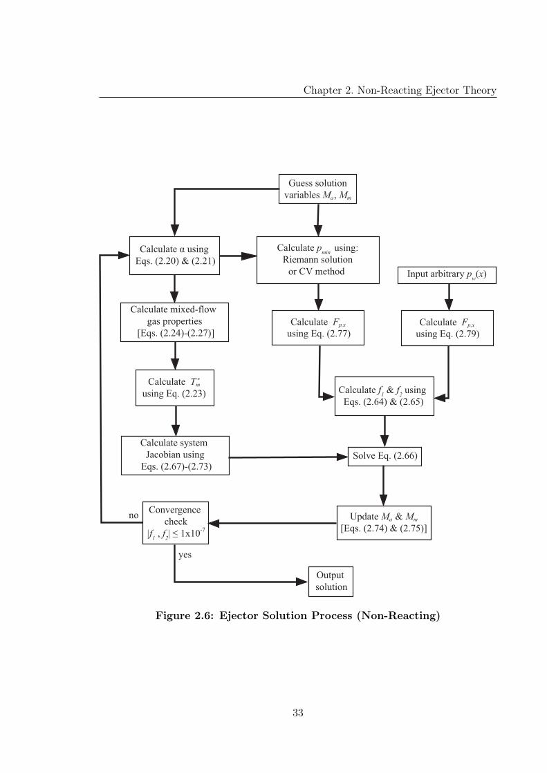
A flowchart representation of the solution process is shown in Figure 2.6. When the
initial guesses for Ma and Mm are set to 0.2 and 0.8 respectively, a converged solution
can be obtained in less than 15 iterations.
Several options exist for computing Fp,x with the choice coming down to what
pressure distribution is used. In either case, the same linear nozzle contour function
will be used whose profile can be expressed as,
r(x) = ri +
(dr
dx
)x (2.76)
When the pressure distribution is defined by Eq. (2.29), one needs to solve for pmin
before Fp,x can be computed. This means that either the CV or Riemann solution
is implemented first using the value of Ma at the given iteration level. Once pmin is
known, one can integrate Equation (2.63) to obtain a closed form expression for Fp,x.
Accordingly, Eqs. (2.29) & (2.76) are substituted into Eq. (2.63) and integrated,
32
Chapter 2. Non-Reacting Ejector Theory
Calculate pmin
using:
Riemann solution
or CV method
Solve Eq. (2.66)
Update Ma & Mm
[Eqs. (2.74) & (2.75)]
Convergence
check
|f1 , f
2| ≤ 1x10
-7
Output
solution
yes
no
Guess solution
variables Ma, Mm
Calculate α using
Eqs. (2.20) & (2.21)
Calculate mixed-flow
gas properties
[Eqs. (2.24)-(2.27)]
Calculate Tm
using Eq. (2.23)
Calculate Fp,x
using Eq. (2.77)
Input arbitrary pw(x)
Calculate Fp,x
using Eq. (2.79)
Calculate system
Jacobian using
Eqs. (2.67)-(2.73)
Calculate f1 & f
2 using
Eqs. (2.64) & (2.65)
Figure 2.6: Ejector Solution Process (Non-Reacting)
33
Chapter 2. Non-Reacting Ejector Theory
giving,
Fp,x =−2πL dr
dx
pmAm
√1 +
(drdx
)2
[pm
2(2ri + rm) − c1c2
6(4ri + rm) +
c130
(6ri + rm)
](2.77)
which is specific to the polynomial-based pressure distribution. If one wishes to use
an arbitrary pw(x) the most convenient method of solution is numerical integration.
The second-order accurate trapezoidal rule will be used in the present case which can
be expressed for an arbitrary function as,
∫ b
a
f(x)dx ≈ ∆x
[f(b) − f(a)
2+
n∑
i=1
f(xi)
](2.78)
Applying the above method to equation (2.63) gives the following numerical formula:
Fp,x ≈ −2π∆x
pmAm
[K(L) −K(0)
2+
n∑
i=1
K(xi)
](2.79)
where
K(x) =pw(x)√
1 + (dr/dx)2r(x)
dr
dx
while centered differencing can be used to evaluate the derivative dr/dx,
dr
dx≈ ri+1 − ri−1
2∆x(2.80)
2.4.1 CV Method - Numerical Solution
The solution of the equations which govern pmin is carried out using the Newton-
Raphson method. The procedure itself is analogous to the method used for Eqs.
(2.4) and (2.16) since both equation sets contain a wall pressure integral. In this
case, Eq. (2.20) can once again be used to rewrite Eqs. (2.36) and (2.43) in the
34
Chapter 2. Non-Reacting Ejector Theory
following form:
f1,CV = (χr,i − χr,2) + ψ√θΓ
(µa,i
µr,i
)(χa,i − χa,2) − Fp,x2 = 0 (2.81)
f2,CV = Aa,iµa,i
µa,2
+ Ar,iµr,i
µr,2
− A(x2) = 0 (2.82)
where the term A(x2) is calculated from the radial contour of the nozzle defined by
equation (2.76). To define the Jacobian, one can differentiate equations (2.81) and
(2.82) with respect to the solution variables (Mr2,Ma2) to obtain,
∂f1,CV
∂Mr,2
= − ∂χr,2
∂Mr,2
∂f1,CV
∂Ma,2
= −α√θΓ
∂χa,2
∂Ma,2
(2.83)
∂f2,CV
∂Mr,2
= −Ar,iµr,i
µ2r,2
∂µr,2
∂Mr,2
∂f2,CV
∂Ma,2
= −Aa,iµa,i
µ2a,2
∂µa,2
∂Ma,2
(2.84)
Solution of the above system also requires that Fp,x2 be related to the solution vari-
ables. Since pmin is found only for the polynomial pressure distribution (Eq. (2.29)),
it is worthwhile to obtain a closed form expression for Fp,x2 as well. Carrying out the
integration gives,
Fp,x2 =−2π dr
dx
mra∗r
√1 +
(drdx
)2
[pminx2
(ri +
x2
2
dr
dx
)+ ric1L
(c22 −
2
3c2
− 8
15c5/2
2 +1
5
)+
dr
dxc1L
2
(c222− c2
6+
1
30− 8
15c5/2
2 +c326
)](2.85)
where x2 is defined by Eq. (2.38). To ensure that the solution process remains stable,
one can introduce a damping factor, ΥCV as,
Mk+1a,2 = Mk
a,2 + ΥCV [∆Ma,2]k (2.86)
Mk+1r,2 = Mk
r,2 + ΥCV [∆Mr,2]k (2.87)
35
Chapter 2. Non-Reacting Ejector Theory
Although more rigorous methods are available for choosing a value for ΥCV , a value
of 0.1 was found to work well. The damping is conditional and is applied only if the
following condition is met:
||(f1,CV , f2,CV )||k+1 ≥ ||(f1,CV , f2,CV )||k (2.88)
which is simply a mathematical condition that represents the solution diverging. The
convergence tolerance in this case is set to,
|f1,CV , f2,CV | ≤ 1 × 10⁻⁷
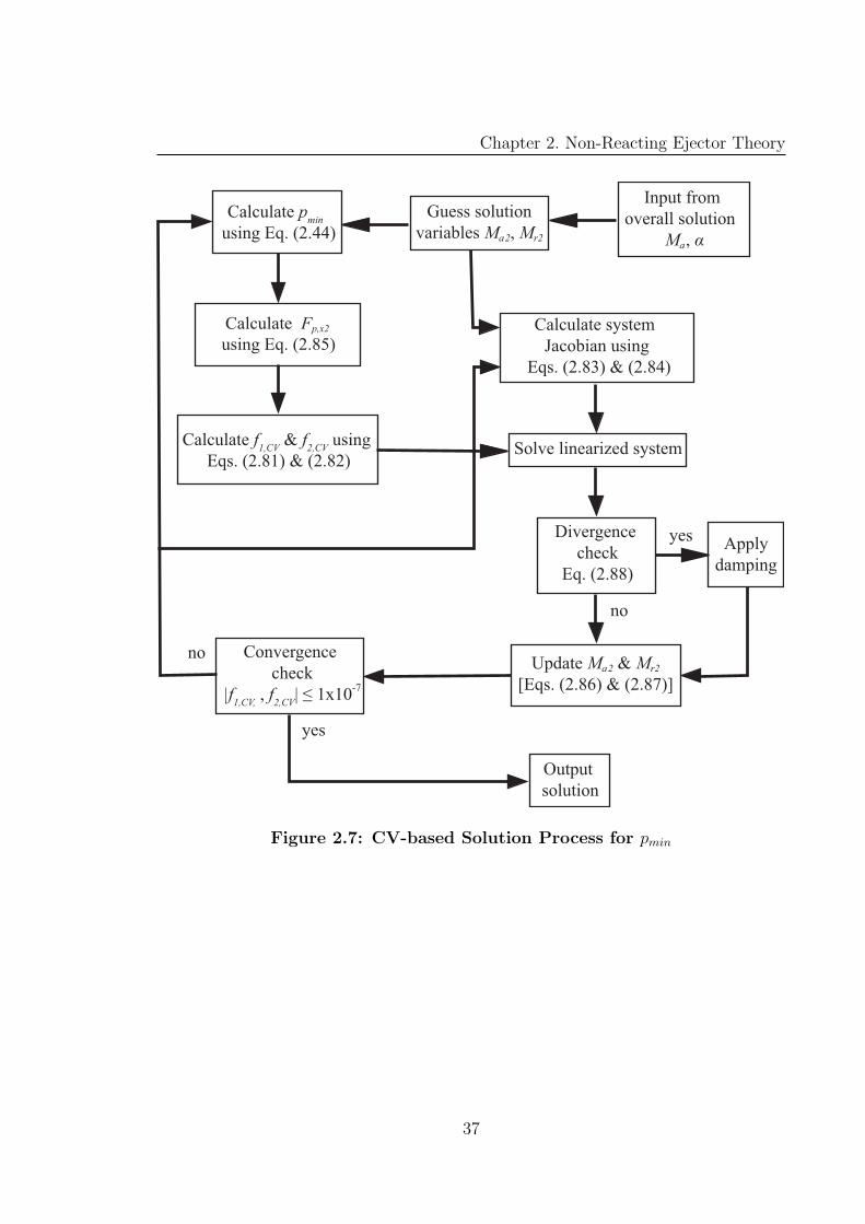
The solution process for pmin is summarized in Figure 2.7 and is invoked at each
iteration level of the solution for the entire ejector (see Fig. 2.6). This means that
a converged solution for pmin is obtained at every iteration of the overall solution
process. The initial guesses for Ma,2 and Mr,2 are set to Ma and 1.2×Mr respectively
and yield a converged solution in less than 220 iterations.
36
Chapter 2. Non-Reacting Ejector Theory
Calculate pmin
using Eq. (2.44)
Solve linearized system
Update Ma2 & Mr2
[Eqs. (2.86) & (2.87)]
Convergence
check
|f1,CV,
, f2,CV
| ≤ 1x10⁻⁷
Output
solution
yes
no
Input from
overall solution
Ma, α
Apply
damping
Calculate Fp,x2
using Eq. (2.85)Calculate system
Jacobian using
Eqs. (2.83) & (2.84)
Calculate f1,CV
& f2,CV
using
Eqs. (2.81) & (2.82)
Guess solution
variables Ma2, Mr2
Divergence
check
Eq. (2.88)
yes
no
Figure 2.7: CV-based Solution Process for pmin
37
Chapter 2. Non-Reacting Ejector Theory
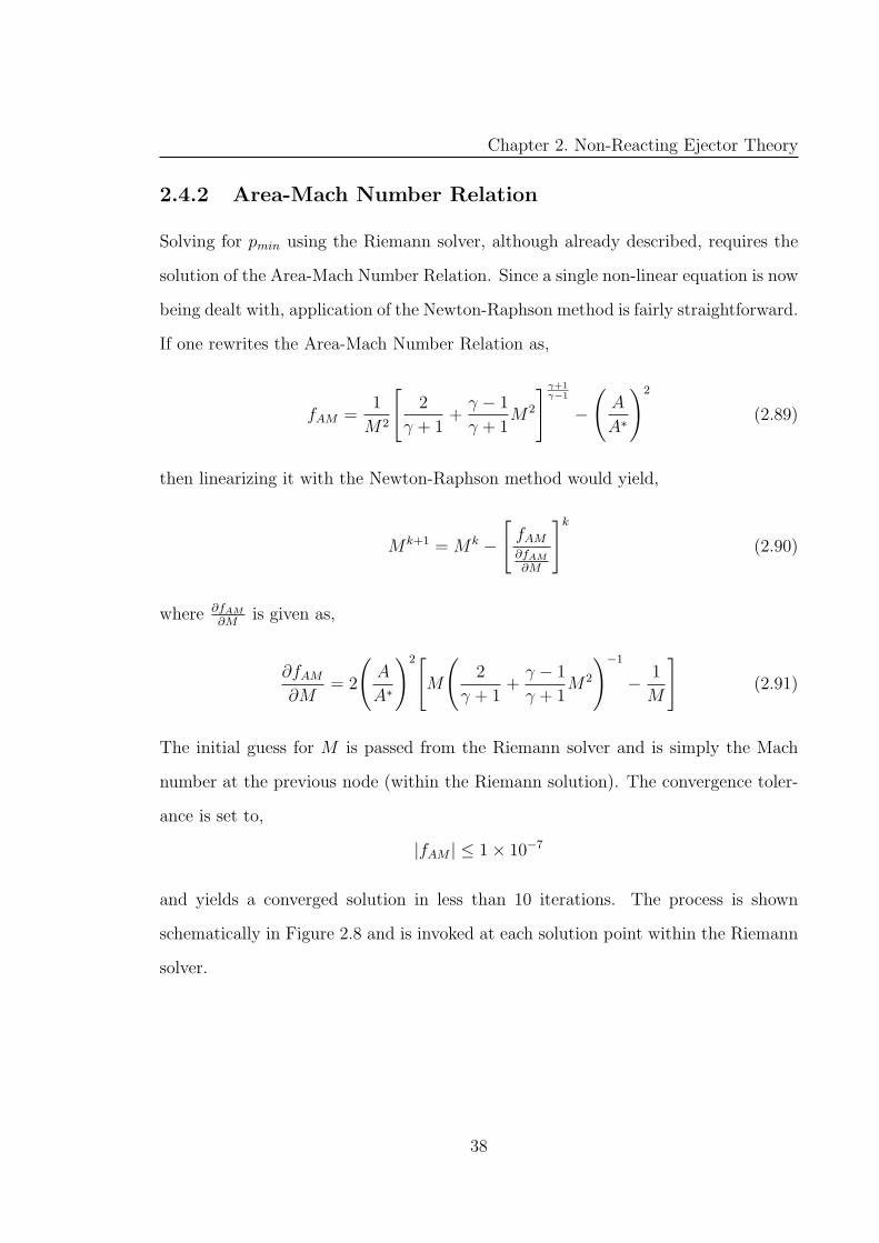
2.4.2 Area-Mach Number Relation
Solving for pmin using the Riemann solver, although already described, requires the
solution of the Area-Mach Number Relation. Since a single non-linear equation is now
being dealt with, application of the Newton-Raphson method is fairly straightforward.
If one rewrites the Area-Mach Number Relation as,
fAM =1
M2
[2
γ + 1+γ − 1
γ + 1M2
] γ+1γ−1
−(A
A∗
)2
(2.89)
then linearizing it with the Newton-Raphson method would yield,
Mk+1 = Mk −[fAM
∂fAM
∂M
]k
(2.90)
where ∂fAM
∂Mis given as,
∂fAM
∂M= 2
(A
A∗
)2[M
(2
γ + 1+γ − 1
γ + 1M2
)−1
− 1
M
](2.91)
The initial guess for M is passed from the Riemann solver and is simply the Mach
number at the previous node (within the Riemann solution). The convergence toler-
ance is set to,
|fAM | ≤ 1 × 10⁻⁷
and yields a converged solution in less than 10 iterations. The process is shown
schematically in Figure 2.8 and is invoked at each solution point within the Riemann
solver.
38
Chapter 2. Non-Reacting Ejector Theory
Solve Eq. (2.90)
and update M
Convergence
check
|fAM
| ≤ 1x10⁻⁷
Output
solution
Calculate
∂ fAM
/∂M
using Eq. (2.91)
Calculate fAM
using Eq. (2.89)
Guess solution
variable M
yes
no no
Figure 2.8: Solution of Area-Mach Number Relation
39
Chapter 3
Theory for SMC Ejector
If one assumes that the pressure distribution used for the unreacting case remains
valid under SMC conditions then the equations for the conservation of mass (Eq.
(2.4)) and momentum (Eq. (2.16)) remain unchanged. Thus the only thing required
is that the energy equation be modified to account for the heat release caused by the
secondary combustion inside the ejector. Keeping this in mind one can derive a more
general form of the energy equation as,
ns∑
k=1
Nkhk +Wmu2
m
2
ns∑
k=1
Nk = ma
(ha +
u2a
2
)+ mr
(hr +
u2r
2
)(3.1)
where ns is the number of atomic species being considered. Since chemical reactions
are now present in the system, all enthalpy terms must be expressed relative to a
reference state. Doing so allows the energy fluxes to be written on a mass-basis as
follows:
h+u2
2=
ns∑
k=1
Yk
Wk
ho
f,k + Cp(To − Tref ) (3.2)
40

Chapter 3. Theory for SMC Ejector
In addition, the ideal gas law and the speed of sound can be used to simplify the
kinetic energy term on the left hand side of Eq (3.1) to give,
Wmu2
m
2
ns∑
k=1
Nk =1
2NmγmRuTmM
2m (3.3)
It should be noted at this point, that the kinetic energy term (Eq. (3.3)) does not
usually show up in a combustion analysis since the post-combustion velocity is usually
small. The present application, however, necessitates that this term be included in the
equation since the velocity at the mixed-flow plane of the ejector cannot be considered
small. Substituting Eqs. (3.2) & (3.3) into Eq. (3.1) while invoking the definitions
of α and θ yields the simplified energy equation,
ns∑
k=1
Nkhk +1
2NmγmRuTmM
2m = H (3.4)
where H represents the total energy flowing into the ejector, and is given as,
H = mrCp,rTor
[(αθ + 1) − Tref
T or
(α(Cp,a
Cp,r
)+ 1
)+
1
Cp,rT or
nr∑
k=1
Yr,k
MWk
ho
f,k
](3.5)
The thermal properties of the reacted mixture can be found on a mass weighted
basis, averaging this time over all of the product species to yield,
Cp,m =ns∑
k=1
YkCp,k (3.6)
Wm =ns∑
k=1
Yk
Wk
(3.7)
Rm =Ru
Wm
(3.8)
γm =
(1 − Rm
Cp,m
)−1
(3.9)
41
Chapter 3. Theory for SMC Ejector
Unlike the unreacting case, it is clear at this point that Eq. (3.4) is not sufficient
to close the system of equations by itself. The inclusion of chemical reactions has
essentially added ns unknowns (Nk’s) for which additional relationships are required.
3.1 Gibbs Minimization
Since equation (3.4) is stated very generally, many different methods can be used.
For the present case, the Gibbs Minimization technique [26] will be applied to solve
for the chemical composition at the exit plane (m) of the ejector. The full derivation
of this method is quite involved, and thus only a brief overview will be presented.
Fundamentally, the Gibbs Minimization technique involves minimizing the Gibbs free
energy of all the atomic species considered while being constrained by the need for
of all the atoms involved in the reactions to be conserved. For this reason it goes
beyond the simple assumption of complete combustion, since the species which can
form under those conditions, such as unburned hydrocarbons and radicals can be
accounted for.
To derive the necessary equations, one first needs to consider the Gibbs free energy
of a single species which can be written as,
gk = gof,k +RuTm
[ln
(Nk
Nm
)+ ln
(pm
pref
)](3.10)
while the Gibbs energy of the entire mixture per unit time can be expressed on a
molar basis to give,
G =ns∑
k=1
Nkgk =ns∑
k=1
Nk
{go
f,k +RuTm
[ln
(Nk
Nm
)+ ln
(pm
pref
)]}(3.11)
One can then differentiate the above expression with respect to Nk to obtain the
42
Chapter 3. Theory for SMC Ejector
following simplified result,
dG =ns∑
k=1
gkdNk (3.12)
The conservation of distinct atoms can be expressed in the following form:
ns∑
k=1
ηikNk = bi, i = 1 → na (3.13)
where ηik is the amount of atomic particle i per kmol of species k while bi is the total
inflow rate of atomic particle i. If one further assumes the usual composition for the
entrained air (21% O2 79% N2), then bi can be expressed as,
bi = mr
[nr∑
k=1
ηikYr,k
Wk
+α
Wa
(0.79ηi,N2 + 0.21ηi,O2)
], i = 1 → na (3.14)
where nr is the number of species present in the rocket plume. At this point one can
minimize Eq. (3.11) subject to the constraint of atom conservation (Eq. (3.13)). The
method of Lagrange Multipliers is a perfect candidate for this task since it can be
used to maximize/minimize a function f(x, y) subject to a constraint function q(x, y).
For multiple constraints, the method generalizes to,
∇f(xo, yo) =∑
k
λk∇qk(xo, yo) (3.15)
where λk is a Lagrange multiplier. Taking the derivative of Eq. (3.13) with respect
to Nk and substituting it along with Eq. (3.12) into the Lagrange formula gives,
gk −na∑
i=1
λiηik = 0, k = 1 → ns (3.16)
where na is the number of distinct atomic species. It is also convenient at this point
43
Chapter 3. Theory for SMC Ejector
to non-dimensionalize the above equation by dividing it by RuTm to give,
gk −na∑
i=1
λiηik = 0, k = 1 → ns (3.17)
where
gk =gk
RuTm
λi =λi
RuTm
(3.18)
Solution of the ejector under SMC conditions can be done in a manner similar to the
unreacting case except that Eq. (2.23) has now been replaced with Eqs. (3.4), (3.13)
and (3.17). Unlike the unreacting case, however, there are now additional (na + ns)
unknowns which are required to solve for the equilibrium composition.
3.2 Numerical Solution
To solve for the post-combustion ejector composition in an efficient manner requires
a slightly unintuitive approach since the solution depends on the number of product
species. For example, if one tried to solve the system using the Newton-Raphson
method with the unknowns being the molar flow rates of the product species (Nk’s),
one would be required to derive and evaluate an ns × ns Jacobian, which would
quickly become cumbersome and inefficient for large numbers of species. In addi-
tion, one would also loose some flexibility since the numerical scheme would need
major modifications for different numbers of product species. In the present case, the
Newton-Raphson method can still be applied, but in a slightly different manner. The
solution methodology that will be shown is adapted from reference [26]. The starting
point for this method is to apply the Newton-Raphson linearization to a generic func-
tional, fs while using the natural logarithm of Nm, Tm and the Nk’s as the solution
44
Chapter 3. Theory for SMC Ejector
variables,
ns∑
k=1
[∂fs
∂ ln(Nk)
]+
∂fs
∂ ln(Nm)∆ ln(Nm) +
∂fs
∂ ln(Tm)∆ ln(Tm) = −fs (3.19)
Using the following mathematical definition
∂y
∂ lnx= x
∂y
∂x
along with Eq. (3.17) as the fs in equation (3.19), one obtains,
∆ ln(Nk) = ∆ ln(Nm) + hk∆ ln(Tm) − gk +na∑
i=1
λiηik, k = 1 → ns (3.20)
with
hk =hk
RuTm
(3.21)
In a similar manner, one can also substitute the atomic constraint equation (Eq.
(3.13)) into Eq. (3.19) to give,
ns∑
k=1
[Nkηik∆ ln(Nk)] = −ns∑
k=1
ηikNk + bi, i = 1 → na (3.22)
At this point the ∆ lnNk term can be eliminated from equation (3.20) by using Eq.
(3.22), resulting in the following expression:
na∑
j=1
{ns∑
k=1
ηikNkηjk
}λj +
{ns∑
k=1
ηikNk
}∆ ln(Nm), i = 1 → na
+
{ns∑
k=1
ηikNkhk
}∆ ln(Tm) = bi −
ns∑
k=1
ηikNk +ns∑
k=1
ηikNkgk (3.23)
Equation (3.23) is an important result since it effectively eliminates the Nk’s from
the numerical procedure and thus significantly improves the computational efficiency
45
Chapter 3. Theory for SMC Ejector
of the method.
For the present solution it is convenient to consider the total molar flow rate, Nm,
as an independent variable for which one can write,
ns∑
k=1
Nk −Nm = 0 (3.24)
The above equation is then used as the next functional (fs) while applying the same
procedure as above to give,
na∑
i=1
{ns∑
k=1
ηikNk
}λi +
{ns∑
k=1
Nk −Nm
}∆ ln(Nm)
+
{ns∑
k=1
Nkhk
}∆ ln(Tm) = Nm +
ns∑
k=1
Nk(gk − 1) (3.25)
Using the energy equation (Eq. (3.4)) as the last functional, one obtains the final
equation required to solve the system as,
na∑
i=1
{ns∑
k=1
ηikNkhk
}λi +
{ns∑
k=1
Nkhk + EK
}∆ ln(Nm)
+
{ns∑
k=1
Nk
[Cp,k
Ru
+ h2k
]+ EK
}∆ ln(Tm)
= H − EK +ns∑
k=1
Nkhk(gk − 1) (3.26)
where
EK =1
2NmγmM
2m (3.27)
H =H
RuTm
(3.28)
Equations (3.23), (3.25) and (3.26) can be expressed in the familiar matrix form
46
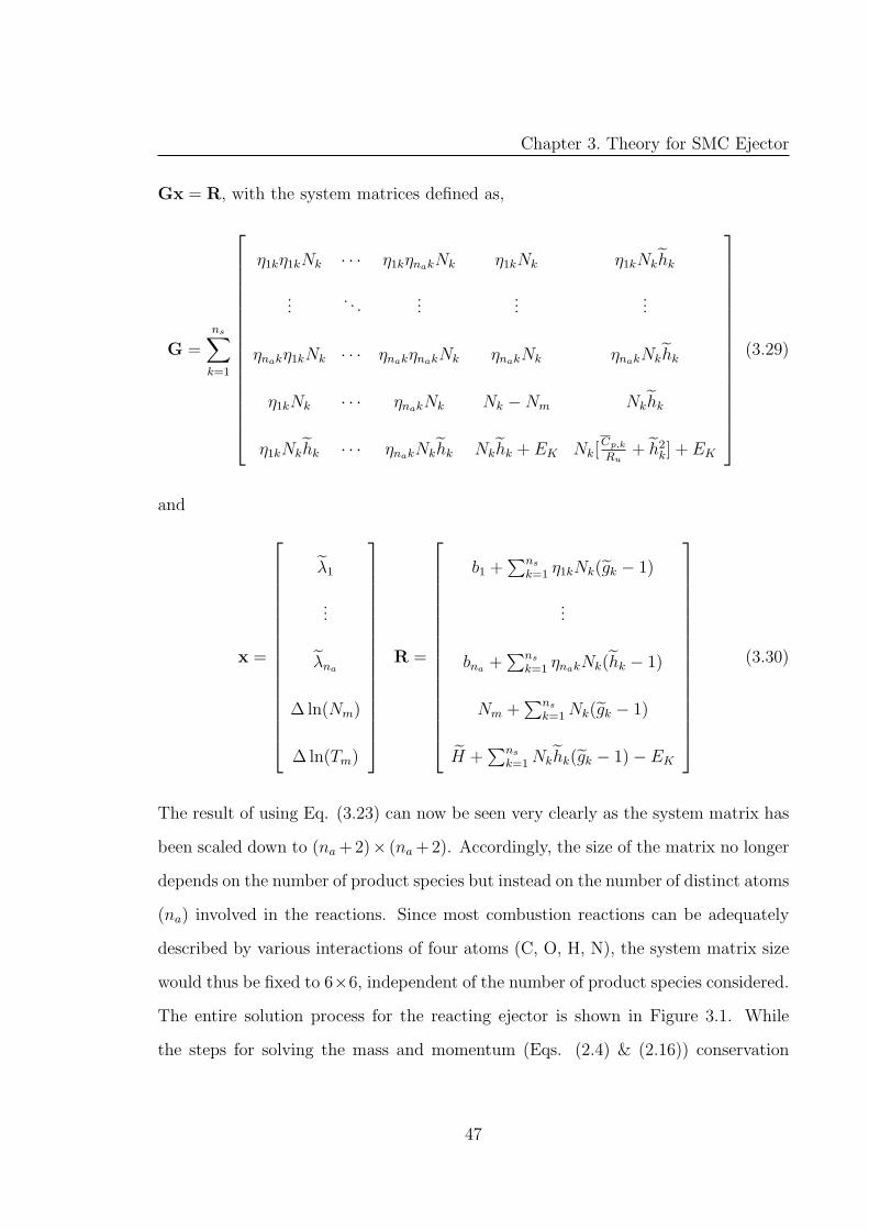
Chapter 3. Theory for SMC Ejector
Gx = R, with the system matrices defined as,
G =ns∑
k=1
η1kη1kNk · · · η1kηnakNk η1kNk η1kNkhk
.... . .
......
...
ηnakη1kNk · · · ηnakηnakNk ηnakNk ηnakNkhk
η1kNk · · · ηnakNk Nk −Nm Nkhk
η1kNkhk · · · ηnakNkhk Nkhk + EK Nk[Cp,k
Ru+ h2
k] + EK
(3.29)
and
x =
λ1
...
λna
∆ ln(Nm)
∆ ln(Tm)
R =
b1 +∑ns
k=1η1kNk(gk − 1)
...
bna+∑ns
k=1ηnakNk(hk − 1)
Nm +∑ns
k=1Nk(gk − 1)
H +∑ns
k=1Nkhk(gk − 1) − EK
(3.30)
The result of using Eq. (3.23) can now be seen very clearly as the system matrix has
been scaled down to (na +2)× (na +2). Accordingly, the size of the matrix no longer
depends on the number of product species but instead on the number of distinct atoms
(na) involved in the reactions. Since most combustion reactions can be adequately
described by various interactions of four atoms (C, O, H, N), the system matrix size
would thus be fixed to 6×6, independent of the number of product species considered.
The entire solution process for the reacting ejector is shown in Figure 3.1. While
the steps for solving the mass and momentum (Eqs. (2.4) & (2.16)) conservation
47
Chapter 3. Theory for SMC Ejector
equations remain the same, solving for the composition involves the inversion of the
G matrix starting from an initial guess at the equilibrium composition (Nm, Nk’s)
and the post-combustion temperature (Tm). The initial guesses used for the present
case are,
Tm = 2500K, Nk = 0.1/ns, k = 1 → ns
The updated values for the solution variables (λk, Nm, Tm) are then used to solve for
all of the Nk’s by applying Eq. (3.20) in a sequential manner. Once a solution for
the composition and Tm is obtained the rest of the ejector solution process continues
in the same manner as for the unreacting case (Fig. 3.1). The entire ejector solution
under SMC conditions is considered converged when the following conditions are met:
|f1, f2| ≤ 1 × 10⁻⁷,ns∑
k=1
Nk −Nm ≤ 1 × 10⁻⁷
In most cases, a converged solution can be obtained in approximately 20 iterations.
To ensure that the numerical procedure remains stable, a damping function is
applied to the equilibrium solution at each iteration. For the major species whose
∆ ln(Nk) is positive, one can calculate the damping factor, Υ1, as,
Υ1 =2
max[|∆ ln(Tm)|, |∆ ln(Nm)|, |∆ lnNk|](3.31)
While for the minor species (Yk ≤ 1 × 10⁻⁸ [26]) with positive ∆ ln(Nk)’s one can
calculate another damping factor,
Υ2 =ln(1 × 10⁻⁴) − ln(Nk) + ln(Nm)
∆ ln(Nk) − ∆ ln(Nm)(3.32)
48
Chapter 3. Theory for SMC Ejector
From Υ1 and Υ2 one can then calculate the overall damping factor,
Υ = min[1,Υ1,Υ2] (3.33)
The damping factor can then be used to update the solution variables,
[ln(Tm)]k+1 = [ln(Tm)]k + Υ[∆ ln(Tm)]k (3.34)
[ln(Nm)]k+1 = [ln(Nm)]k + Υ[∆ ln(Nm)]k (3.35)
[ln(Nk)]k+1 = [ln(Nk)]
k + Υ[∆ ln(Nk)]k k = 1 → ns (3.36)
49
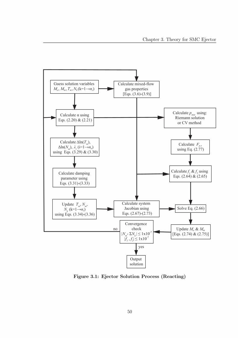
Chapter 3. Theory for SMC Ejector
Calculate pmin
using:
Riemann solution
or CV method
Solve Eq. (2.66)
Update Ma & Mm
[Eqs. (2.74) & (2.75)]
Convergence
check
|Nm- ΣN
k | ≤ 1x10
-7
|f1 , f
2| ≤ 1x10
-7
Output
solution
yes
no
Guess solution variables
Ma, Mm, Tm, Nk (k=1→ns)
Calculate α using
Eqs. (2.20) & (2.21)
Calculate mixed-flow
gas properties
[Eqs. (3.6)-(3.9)]
Calculate Fp,x
using Eq. (2.77)
Calculate system
Jacobian using
Eqs. (2.67)-(2.73)
Calculate f1 & f
2 using
Eqs. (2.64) & (2.65)
Calculate Δln(Tm),
Δln(Nm),
λ
i (i=1→na)
using Eqs. (3.29) & (3.30)
Update Tm, N
m,
N
k (k=1→ns)
using Eqs. (3.34)-(3.36)
Calculate damping
parameter using
Eqs. (3.31)-(3.33)
Figure 3.1: Ejector Solution Process (Reacting)
50
Chapter 4
Partially Mixed Ejector Theory
The theory for the partially mixed ejector is essentially an extension of the fully-mixed
theory presented earlier. The scope of the problem is quite broad since all of the flow
variables at a given plane will not be uniform for a flow that is not fully mixed.
To simplify the analysis, the variation of T, ρ, p and R in the radial direction will
therefore be neglected. The only variable that will be allowed to vary is the velocity
u. With this notion, the conservation of mass is applied to the ejector control volume
shown in Fig. 2.1 to yield,
mr + ma = 2π
∫ rm
0
ρurdr (4.1)
Since the density at the mixed flow plane was assumed to be uniform, it can be taken
out of the integral. One can then simplify the equation by using the definition of α
to give,
mr
Am
(α+ 1) = ρmum (4.2)
where um is the area-averaged velocity, defined as,
um =2
r2m
∫ rm
0
urdr (4.3)
51
Chapter 4. Partially Mixed Ejector Theory
Before the mass conservation equation can be simplified further, one needs to derive
the energy equation, which can be written as follows:
maCp,aToa + mrCp,rT
or = 2π
∫ rm
0
ρu(Cp,mT + u2/2)rdr (4.4)
The left hand side of the above equation can be simplified in the same manner as for
the fully mixed case, by invoking the definitions of α and θ. Furthermore, the integral
on the right hand side can be split since the temperature does not vary with r. The
result can then be divided by Am to give,
mrCp,rTor (αθ + 1) = ρmAm
[Cp,mTm
2
r2m
∫ rm
0
urdr
︸ ︷︷ ︸um
+1
r2m
∫ rm
0
u3rdr
]
If one then multiplies and divides the equation by u3m, one obtains,
mrCp,rTor (αθ + 1) = ρmAmumCp,m
[Tm + βe
u3m
Cp,m
]
where βe is the energy mixing factor, given as,
βe =1
u3mr
2m
∫ rm
0
u3rdr (4.5)
At this point it is convenient to define the area-averaged total temperature,
To
m = Tm + βeu2
m
Cp,m
(4.6)
If one further defines the area-averaged Mach number as,
Mm =um
γmRmTm
(4.7)
52
Chapter 4. Partially Mixed Ejector Theory
then Eq. (4.6) can be written in the following form:
To
m = Tm(1 + (γm − 1)βeM2
m) (4.8)
Equations (4.2) and (4.8) can now be substituted into the energy equation, to give
the final result,
To
m =Cp,r
Cp,m
(αθ + 1)
(α+ 1)T o
r (4.9)
To finish deriving the mass conservation equation, one needs to restate it in terms
of Mm by multiplying and dividing Eq. (4.10) by the speed of sound and using the
ideal gas law to give,
mr
Am
(α+ 1) = pm
√γm
RmTm
Mm
One can then substitute Eq. (4.8) into the above expression to obtain the final result,
mr
pmAm
√RmT
o
m
γm
(α+ 1) = Mm
(1 + (γm − 1)βeM
2
m
)1/2
(4.10)
To complete the equation set, one can now apply the momentum equation, which can
be written as,
(maua+paAa)+(mrur+prAr)−pmAm−∫∫ L
0
pw(x) · d~Sx =
[2π
∫ rm
0
ρu2rdr
](4.11)
The left hand side of the equation above can be simplified in the same manner as
Eq. (2.6) while using the ideal gas law on the right hand side to give the following
expression:
mra∗
r
pmAm
(α√θΓχa + χr) − Fp,x − 1 =
1
RmTm
[2
r2m
∫ rm
0
u2rdr
]
53
Chapter 4. Partially Mixed Ejector Theory
The above result can then be divided and multiplied by u2m while using Eq. (4.7) to
get,
M2
m =1
γmβm
[mra
∗
r
pmAm
(α√θΓχa + χr) − Fp,x − 1
](4.12)
where βm is the momentum mixing factor, defined as,
βm =2
u2mr
2m
∫ rm
0
u2rdr (4.13)
Finally, Eqs. (2.24)-(2.27) will be used to solve for the gas properties at the mixed-
flow plane of the ejector.
To summarize, the foregoing analysis has yielded three equations which govern
the partially mixed ejector. Upon inspection of Eqs. (4.9), (4.10) & (4.12) it is easy
to see that they are nearly identical in form to the equations for the fully-mixed
case ((2.4), (2.16) & (2.23)). Since the major departure from the fully-mixed theory
was the treatment of the mixed-flow plane (Mm → Mm, etc), all previously defined
equations for the µ and χ functionals (Eqs. (2.3) (2.10)) apply in this case as well.
Consequently, if one can obtain expressions for the two mixing factors, βm and βe
then Eqs. (4.9), (4.10) & (4.12) can be solved in exactly the same manner as the
equations for the fully mixed ejector.
4.1 Mixed-Flow Velocity Profile
To properly quantify the two mixing factors, one needs to assume an appropriate
velocity profile at the mixed-flow plane of the ejector. In the current treatment,
the boundary layer at the mixed-flow plane will be neglected since the intent is to
only model the mixing. In addition, since the model is specific to the annular rocket
configuration, it can be further assumed that the upper boundary of the shear layer
will quickly spread out toward the upper wall. Use of this assumption allows one to
54

Chapter 4. Partially Mixed Ejector Theory
split the velocity profile into two regions, a shear layer region, which extends from
the top wall down, as well as a uniform flow region which extends from the centerline
up to the lower boundary of the shear layer.
00
1
1u/u1
r/rm
ǫ
u2/u1 Uniform Flow Region
u/u1 = f(ξ)
Shear Layer Region
Figure 4.1: Assumed Velocity Profile at Mixed-Flow Plane
A schematic of the composite profile is presented in Figure 4.1, where ǫ is a relative
shear layer thickness defined as,
ǫ =δmrm
(4.14)
To facilitate the use of specific empirical correlations, it is convenient to express
this profile as a function of u2 which is the velocity at the lower boundary of the
shear layer. One can then make use of the fact that a similarity profile exists for
a compressible turbulent shear layer, provided that proper scaling is used for non-
dimensionalization. The velocity scale is generally taken as the velocity at either
one of the shear layer boundaries, while the shear layer thickness, δm is used as the
length scale. Curve fits for the profile typically involve the well-known Gaussian error
function [34]. Although very good agreement between experimental data is obtained
when this function is used, it cannot be readily integrated. For this reason, the
55
Chapter 4. Partially Mixed Ejector Theory
similarity profile will be approximated by using a cubic polynomial of the form:
u(r) = co + c1r + c2r2 + c3r
3 (4.15)
If one applies the following boundary conditions:
u(rm) = u1,du
dr(rm) = 0, u(rm − δm) = u2,
du
dr(rm − δm) = 0
to Eq. (4.15), then the velocity profile can obtained as,
u
u1
= u∗ + (1 − u∗)(3 − 2ξ)ξ2 (4.16)
where u∗ is defined as,
u∗ =u2
u1
(4.17)
and
ξ =r − (rm − δm)
δm(4.18)
Equation (4.16) can then be integrated to yield the expressions required to solve
for the integrals appearing in equations (4.3), (4.5) & (4.13).
∫ rm
0
urdr =u1r
2m
2
{(1 − ǫ)2u∗ +
ǫ
10(u∗(10 − 7ǫ) + (10 − 3ǫ))
}(4.19)
∫ rm
0
u2rdr =u2
1r2m
2
{(1 − ǫ)2u∗2 +
ǫ
35[2u∗2(13 − 10ǫ)
+9u∗(2 − ǫ) + 2(13 − 3ǫ)]
}(4.20)
56
Chapter 4. Partially Mixed Ejector Theory
∫ rm
0
u3rdr =u3
1r2m
4
{(1 − ǫ)2u∗3 +
ǫ
3080[u∗3(946 − 763ǫ)
+u∗2(594 − 351ǫ) + u∗(594 − 243ǫ) + (946 − 183ǫ)]
}(4.21)
4.2 Mixing Correlations
To be able to use Eqs (4.19)-(4.21), additional relations are needed to define u∗ and ǫ
at the mixed-flow plane of the ejector. Accurately modeling a compressible turbulent
shear layer is a difficult task, even with modern computational tools. In addition,
the shear layer is also axisymmetric and thus fundamentally different [64] from a
simpler, planar case for which most experimental data is available. Since the present
model is fairly simple, it lends itself to the use of empirical correlations for plane
mixing layers. Although some deviation will be expected, the essential physics of
compressible, turbulent mixing will be retained.
The first quantity that is required is the width of the shear layer. One can estimate
δm by using a correlation for its growth rate. For a planar, compressible, turbulent
shear layer, Papamoschou [57] gives the correlation as,
dδ
dx=
0.085(1 + ν)(1 − τ)
1 + ντf(Mc) (4.22)
where
ν =ρr
ρa
(4.23)
and
τ =ur
ua
(4.24)
The function f(Mc) accounts for the effects of compressibility and is estimated by
57

Chapter 4. Partially Mixed Ejector Theory
the following empirical relation,
f(Mc) = 0.25 + 0.75e−3M2c (4.25)
where Mc is the convective Mach number,
Mc =ur − ua
ar + aa
(4.26)
Since a turbulent shear layer grows linearly [64] (Eq. (4.22)), one can estimate the
shear layer thickness at the mixed-flow plane using,
δm ≈ Ldδ
dx(4.27)
10
0 u/ur
r
raua
ri
ur
Figure 4.2: Velocity Profile at Ejector Inlet
The last parameter required to quantify the velocity profile is the dimensionless
velocity, u∗. An equation for this quantity can be obtained from Alber and Lees [1],
and is written as,
x
sθθo
=19.7u∗3
2 − u∗ − 4u∗2(4.28)
58
Chapter 4. Partially Mixed Ejector Theory
where sθ is a spreading parameter based on the momentum thickness. It is related to
the usual turbulent spreading parameter s by the following equation:
sθ
s= [1 + [(γm − 1)/2]M
2
m]2 (4.29)
In the present work the generally accepted value of s = 9.42 [1] is used. Although
Eq. (4.28) can give u∗ at any x-location, only the value at the mixed-flow plane is
required for the solution.
To be able to use Eq. (4.28), some way of estimating the initial momentum thick-
ness is required. By definition, the compressible version of the momentum thickness
integral can be written as,
θo =
∫ ra
0
(1 − u
ur
) ρu
ρrur
dr (4.30)
To simplify the integration, one can assume uniform velocity profiles at the inlet of
the ejector, as shown in Figure 4.2. Assuming that the density profiles have the same
form, the integral in Eq. (4.30) can be evaluated to yield,
θo =
(τ − 1
ντ 2
)ra (4.31)
4.3 Numerical Solution
As was mentioned earlier, the equations for the partially mixed ejector are nearly
identical to those of the fully mixed case. For this reason, the numerical solution
of those equations can be carried out in the same manner as shown in Figure 2.6
(T om → T
o
m,Mm → Mm). However, due to the addition of the mixing factors, some
modification of the equations as well as the Jacobian is required. Firstly, the mass
59
Chapter 4. Partially Mixed Ejector Theory
and momentum conservation equations can be restated more conveniently as,
f1 = −γmβmM2
m +
[ψmra
∗
r
µrpmAm
√θΓ
]µaχa +
[mra
∗
r
pmAm
χr − Fp,x − 1
]= 0 (4.32)
and
f2 =mr
pmAm
√RmT
o
m
γm
(ψµa
µr
+ 1
)−Mm(1 + (γm − 1)βeM
2
m)1/2 = 0 (4.33)
Since the partially-mixed formulation altered only the mixed-flow plane as compared
to the fully mixed case, all derivatives with respect to Ma remain unchanged. One
does, however, need to alter the derivatives with respect to the area-averaged Mach
number. Differentiating Eqs. (4.32) and (4.33) with respect to Mm one can write,
∂f1
∂Mm
= −2γmβmMm (4.34)
∂f2
∂Mm
= −(1 + (γm − 1)β2M
2
m
)1/2
[(γm − 1)βeM
2
m
2(1 + (γm − 1)βeM2
m)+ 1
](4.35)
which can be substituted in place of Eqs (2.68) and (2.69) to implement the solution
procedure for the partially-mixed model.
60
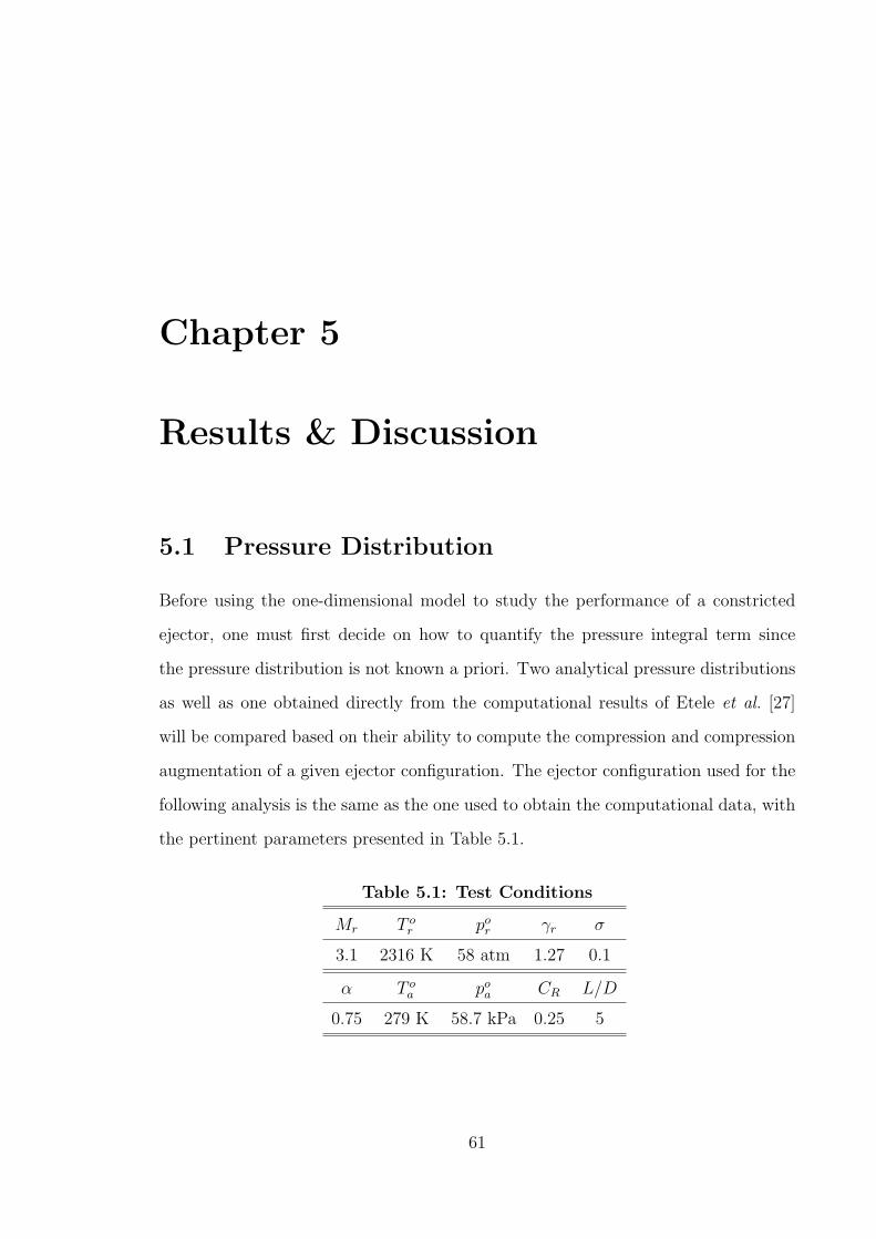
Chapter 5
Results & Discussion
5.1 Pressure Distribution
Before using the one-dimensional model to study the performance of a constricted
ejector, one must first decide on how to quantify the pressure integral term since
the pressure distribution is not known a priori. Two analytical pressure distributions
as well as one obtained directly from the computational results of Etele et al. [27]
will be compared based on their ability to compute the compression and compression
augmentation of a given ejector configuration. The ejector configuration used for the
following analysis is the same as the one used to obtain the computational data, with
the pertinent parameters presented in Table 5.1.
Table 5.1: Test Conditions
Mr T or po
r γr σ
3.1 2316 K 58 atm 1.27 0.1
α T oa po
a CR L/D
0.75 279 K 58.7 kPa 0.25 5
61
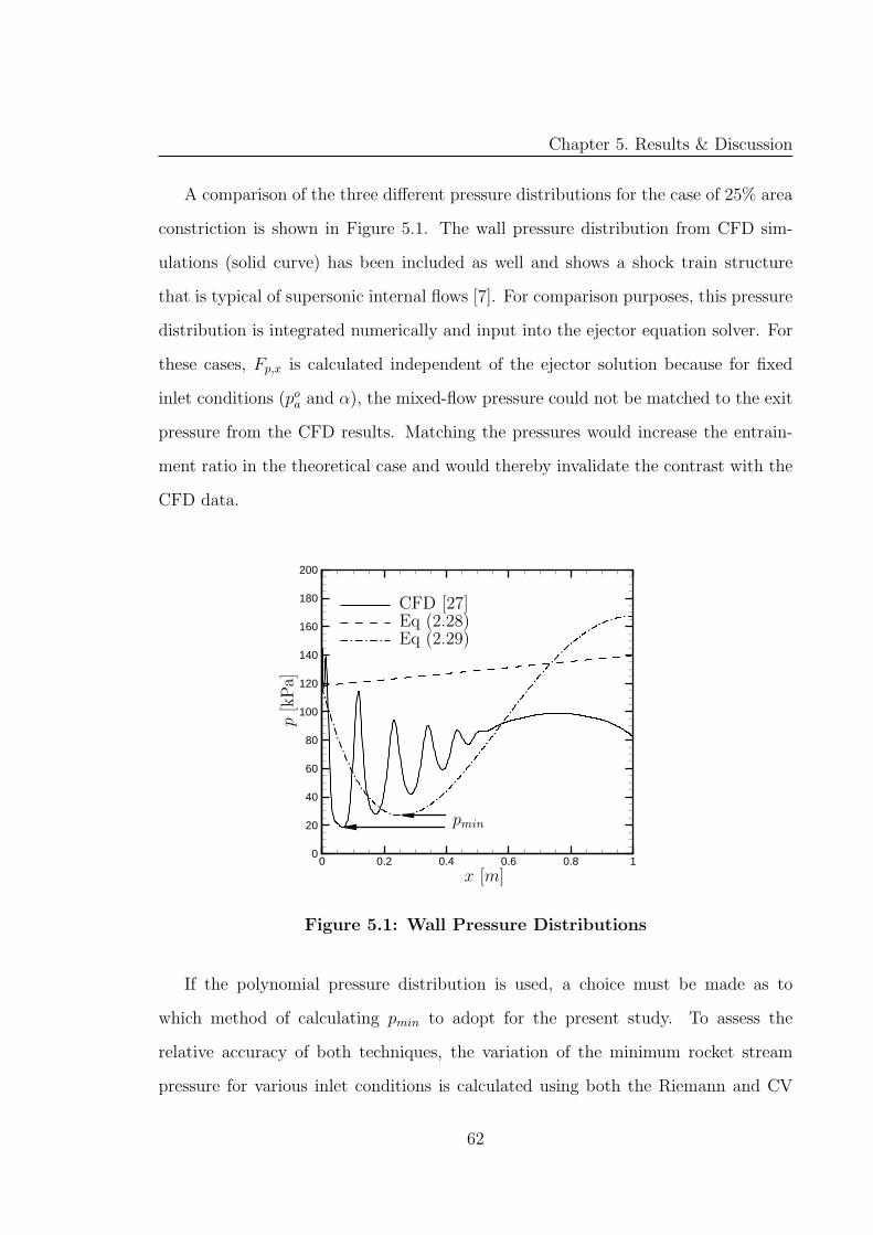
Chapter 5. Results & Discussion
A comparison of the three different pressure distributions for the case of 25% area
constriction is shown in Figure 5.1. The wall pressure distribution from CFD sim-
ulations (solid curve) has been included as well and shows a shock train structure
that is typical of supersonic internal flows [7]. For comparison purposes, this pressure
distribution is integrated numerically and input into the ejector equation solver. For
these cases, Fp,x is calculated independent of the ejector solution because for fixed
inlet conditions (poa and α), the mixed-flow pressure could not be matched to the exit
pressure from the CFD results. Matching the pressures would increase the entrain-
ment ratio in the theoretical case and would thereby invalidate the contrast with the
CFD data.
0 0.2 0.4 0.6 0.8 10
20
40
60
80
100
120
140
160
180
200
x [m]
p[k
Pa]
CFD [27]Eq (2.28)Eq (2.29)
pmin
Figure 5.1: Wall Pressure Distributions
If the polynomial pressure distribution is used, a choice must be made as to
which method of calculating pmin to adopt for the present study. To assess the
relative accuracy of both techniques, the variation of the minimum rocket stream
pressure for various inlet conditions is calculated using both the Riemann and CV
62
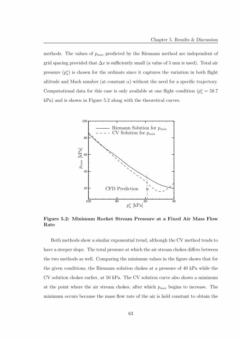
Chapter 5. Results & Discussion
methods. The values of pmin predicted by the Riemann method are independent of
grid spacing provided that ∆x is sufficiently small (a value of 5 mm is used). Total air
pressure (poa) is chosen for the ordinate since it captures the variation in both flight
altitude and Mach number (at constant α) without the need for a specific trajectory.
Computational data for this case is only available at one flight condition (poa = 58.7
kPa) and is shown in Figure 5.2 along with the theoretical curves.
406080100
20
40
60
80
100
poa [kPa]
p min
[kPa]
CV Solution for pmin
Riemann Solution for pmin
CFD Prediction
Figure 5.2: Minimum Rocket Stream Pressure at a Fixed Air Mass FlowRate
Both methods show a similar exponential trend, although the CV method tends to
have a steeper slope. The total pressure at which the air stream chokes differs between
the two methods as well. Comparing the minimum values in the figure shows that for
the given conditions, the Riemann solution chokes at a pressure of 40 kPa while the
CV solution chokes earlier, at 50 kPa. The CV solution curve also shows a minimum
at the point where the air stream chokes, after which pmin begins to increase. The
minimum occurs because the mass flow rate of the air is held constant to obtain the
63
Chapter 5. Results & Discussion
solutions presented in Figure 5.2. Furthermore, since the mass flow rate at sonic
conditions is directly proportional to the flow’s total pressure and sonic throat area,
when poa is decreased A∗
a has to increase. When this occurs the area of the rocket
stream decreases (Ar), which yields a smaller Mr and thus a higher pressure (pmin).
This behaviour makes sense from a physical standpoint, since one would expect the
choking of the air stream to place a lower bound on pmin.
The Riemann solution, on the other hand, does not show the same type of limiting
behaviour, since the choking condition was used to stop the solver before the expan-
sion of the rocket plume was complete. The discrepancy in this case can come from
two sources. The first is the Riemann solver itself, which may be over-estimating the
extent to which the rocket stream can expand. The other option is that the entrain-
ment ratio, which is governed by Eqs. (2.4), (2.16) & (2.23) is being overestimated at
choked airflow conditions. In this case, the Riemann solver may be more representa-
tive of the true flow physics, and the inflow condition being imposed by the governing
equations is unrealistic. In either case it is clear that using the Riemann approach
with the overall ejector solution procedure is producing anomalies when the air flow
chokes, while the CV method seems to be better suited to the present approach.
Overall, both methods are in good agreement with each other due to the common
assumptions used by both techniques. From the figure, it is also clear that both
methods predict a value of pmin that is 60-70% higher than the CFD prediction. The
reason for the discrepancy is tied to the presence of the shear layer which entrains fluid
from both streams and facilitates the transfer of mechanical energy. This causes the
total pressure and the mass flow rate of the rocket stream to decrease as the mixing
progresses, which means that the flow is not isentropic. These facts are clearly evident
in Table 5.2, which shows that both the mass flow rate and the velocity of the rocket
stream in the CFD results are lower than the theoretical values. Another reason is
the fact that the flow in this expansion region is highly two-dimensional and would
64
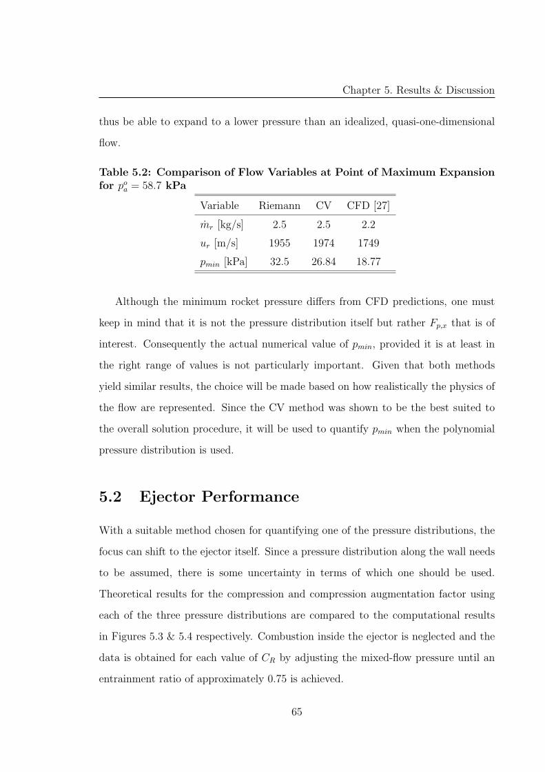
Chapter 5. Results & Discussion
thus be able to expand to a lower pressure than an idealized, quasi-one-dimensional
flow.
Table 5.2: Comparison of Flow Variables at Point of Maximum Expansionfor po
a = 58.7 kPa
Variable Riemann CV CFD [27]
mr [kg/s] 2.5 2.5 2.2
ur [m/s] 1955 1974 1749
pmin [kPa] 32.5 26.84 18.77
Although the minimum rocket pressure differs from CFD predictions, one must
keep in mind that it is not the pressure distribution itself but rather Fp,x that is of
interest. Consequently the actual numerical value of pmin, provided it is at least in
the right range of values is not particularly important. Given that both methods
yield similar results, the choice will be made based on how realistically the physics of
the flow are represented. Since the CV method was shown to be the best suited to
the overall solution procedure, it will be used to quantify pmin when the polynomial
pressure distribution is used.
5.2 Ejector Performance
With a suitable method chosen for quantifying one of the pressure distributions, the
focus can shift to the ejector itself. Since a pressure distribution along the wall needs
to be assumed, there is some uncertainty in terms of which one should be used.
Theoretical results for the compression and compression augmentation factor using
each of the three pressure distributions are compared to the computational results
in Figures 5.3 & 5.4 respectively. Combustion inside the ejector is neglected and the
data is obtained for each value of CR by adjusting the mixed-flow pressure until an
entrainment ratio of approximately 0.75 is achieved.
65
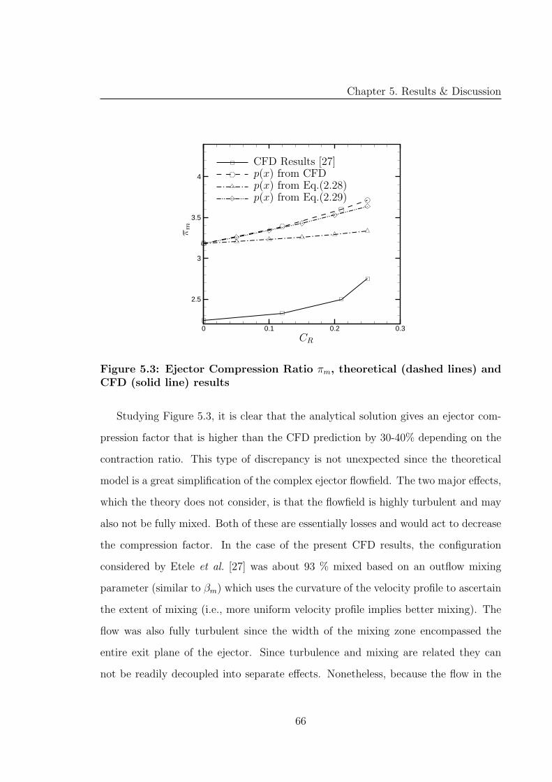
Chapter 5. Results & Discussion
0 0.1 0.2 0.3
2.5
3
3.5
4
CR
πm
CFD Results [27]p(x) from CFDp(x) from Eq.(2.28)p(x) from Eq.(2.29)
Figure 5.3: Ejector Compression Ratio πm, theoretical (dashed lines) andCFD (solid line) results
Studying Figure 5.3, it is clear that the analytical solution gives an ejector com-
pression factor that is higher than the CFD prediction by 30-40% depending on the
contraction ratio. This type of discrepancy is not unexpected since the theoretical
model is a great simplification of the complex ejector flowfield. The two major effects,
which the theory does not consider, is that the flowfield is highly turbulent and may
also not be fully mixed. Both of these are essentially losses and would act to decrease
the compression factor. In the case of the present CFD results, the configuration
considered by Etele et al. [27] was about 93 % mixed based on an outflow mixing
parameter (similar to βm) which uses the curvature of the velocity profile to ascertain
the extent of mixing (i.e., more uniform velocity profile implies better mixing). The
flow was also fully turbulent since the width of the mixing zone encompassed the
entire exit plane of the ejector. Since turbulence and mixing are related they can
not be readily decoupled into separate effects. Nonetheless, because the flow in the
66
Chapter 5. Results & Discussion
computational case is close to being fully mixed, it is clear that turbulence plays a
much more important role.
To examine how well the analytical model predicts air entrainment, it is neces-
sary to match the ejector’s exit conditions (pm) so that the inflow conditions can be
compared. This type of comparison reveals that the theory also predicts a higher sec-
ondary (air) mass flow rate, and thus a higher value of CR at which the entire ejector
chokes. For example, when CR = 0.25, the analytical model predicts an entrainment
ratio that is approximately 52% higher than the CFD results would suggest. This
discrepancy is tied to viscous effects as well as the turbulent nature of the flowfield
which have a strong influence on the shape (or curvature) of the velocity profile and
thus limit the amount of mass that can be passed through a given cross section.
Despite the higher values of πm & α predicted by the analytical model, the trends
are well represented, especially when the wall pressure distribution is defined either
by Eq. (2.29) or obtained directly form the CFD simulations (top two curves). In
fact, in both of these cases, the rate of increase of πm with decreasing exit area
is well captured as shown in Figures 5.3 & 5.4. Comparing the top two curves in
Figure 5.3, it is evident that both give nearly identical results for πm, even though
the mixed-flow pressures for the two distributions (see Fig. 5.1) are quite different.
This is an interesting result, because using the wall pressures extracted from the CFD
simulations to quantify Fp,x represents the accuracy limit of the theoretical integral
analysis. This would seem to suggest that the discrepancy in πm is not caused by the
pressure distribution, but rather by neglecting the effects mentioned earlier. It also
means that within the framework of the theory presented herein, Eq. (2.29) is indeed
a reasonable approximation of the integral of the wall pressure (Fp,x).
If one assumes that the viscous and turbulent effects stay nearly constant with CR,
than they can be effectively eliminated by dividing the compression factors in Fig. 5.3
by [πm]CR=0. The result is the compression augmentation factor, πm, which provides
67
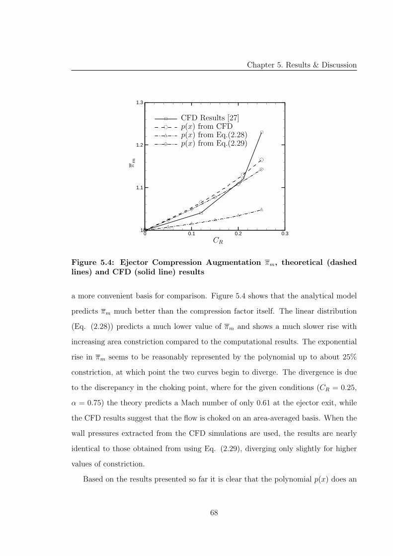
Chapter 5. Results & Discussion
0 0.1 0.2 0.31
1.1
1.2
1.3
CR
πm
CFD Results [27]p(x) from CFDp(x) from Eq.(2.28)p(x) from Eq.(2.29)
Figure 5.4: Ejector Compression Augmentation πm, theoretical (dashedlines) and CFD (solid line) results
a more convenient basis for comparison. Figure 5.4 shows that the analytical model
predicts πm much better than the compression factor itself. The linear distribution
(Eq. (2.28)) predicts a much lower value of πm and shows a much slower rise with
increasing area constriction compared to the computational results. The exponential
rise in πm seems to be reasonably represented by the polynomial up to about 25%
constriction, at which point the two curves begin to diverge. The divergence is due
to the discrepancy in the choking point, where for the given conditions (CR = 0.25,
α = 0.75) the theory predicts a Mach number of only 0.61 at the ejector exit, while
the CFD results suggest that the flow is choked on an area-averaged basis. When the
wall pressures extracted from the CFD simulations are used, the results are nearly
identical to those obtained from using Eq. (2.29), diverging only slightly for higher
values of constriction.
Based on the results presented so far it is clear that the polynomial p(x) does an
68
Chapter 5. Results & Discussion
adequate job of modeling the ejector’s performance within the accuracy limits of the
theoretical analysis. More importantly, the exponential trends in both πm and πm
are reproduced reasonably well up to the choking limit. Due to the convenience of a
closed-form expression, as well as its relative accuracy, Equation (2.29) will be used to
quantify Fp,x for the remainder of this study. It should be kept in mind, however, that
the fully-mixed theory lacks the performance loss mechanisms commonly encountered
in ejectors (viscosity, turbulence). Accordingly, the theoretical values of πm would be
different from a real ejector, and could be on the order of 40%, as is the case for the
present comparison.
5.3 Effects of Combustion
Although good agreement has been seen between theory and CFD, the results pre-
sented so far were obtained at operating conditions which are not representative of
an actual ejector. Specifically, the preceding data was obtained at an unrealistically
low equivalence ratio to avoid combustion and thus allow a comparison under a mix-
ing only basis. This does not occur in practice since rockets are generally operated
at equivalence ratios much higher than 0.2. To investigate the performance of the
ejector in this regime one must now account for the effects of combustion. Since the
SMC mode is of particular interest, one must look at the ejector under fuel rich as
well as fuel lean conditions. A wide operating range such as this necessitates the
need to account for dissociated species as well as products of incomplete combustion.
This makes the Gibbs Minimization technique particularly well suited for this task
as any number of various product species can be assumed to occur. Use of the equi-
librium assumption is warranted for these conditions since it has been validated for
the supersonic flowfield of the rocket using a CFD code which accounts for finite-rate
combustion kinetics [26]. The product species were chosen by consulting the same
69
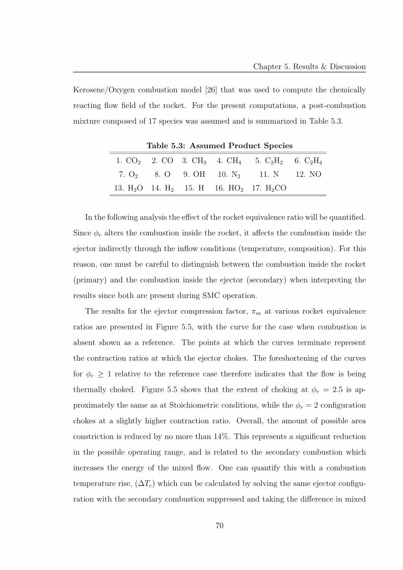
Chapter 5. Results & Discussion
Kerosene/Oxygen combustion model [26] that was used to compute the chemically
reacting flow field of the rocket. For the present computations, a post-combustion
mixture composed of 17 species was assumed and is summarized in Table 5.3.
Table 5.3: Assumed Product Species
1. CO2 2. CO 3. CH3 4. CH4 5. C2H2 6. C2H4
7. O2 8. O 9. OH 10. N2 11. N 12. NO
13. H2O 14. H2 15. H 16. HO2 17. H2CO
In the following analysis the effect of the rocket equivalence ratio will be quantified.
Since φr alters the combustion inside the rocket, it affects the combustion inside the
ejector indirectly through the inflow conditions (temperature, composition). For this
reason, one must be careful to distinguish between the combustion inside the rocket
(primary) and the combustion inside the ejector (secondary) when interpreting the
results since both are present during SMC operation.
The results for the ejector compression factor, πm at various rocket equivalence
ratios are presented in Figure 5.5, with the curve for the case when combustion is
absent shown as a reference. The points at which the curves terminate represent
the contraction ratios at which the ejector chokes. The foreshortening of the curves
for φr ≥ 1 relative to the reference case therefore indicates that the flow is being
thermally choked. Figure 5.5 shows that the extent of choking at φr = 2.5 is ap-
proximately the same as at Stoichiometric conditions, while the φr = 2 configuration
chokes at a slightly higher contraction ratio. Overall, the amount of possible area
constriction is reduced by no more than 14%. This represents a significant reduction
in the possible operating range, and is related to the secondary combustion which
increases the energy of the mixed flow. One can quantify this with a combustion
temperature rise, (∆Tc) which can be calculated by solving the same ejector configu-
ration with the secondary combustion suppressed and taking the difference in mixed
70
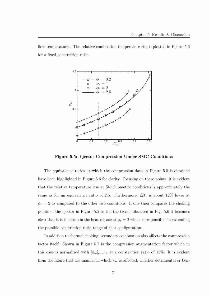
Chapter 5. Results & Discussion
flow temperatures. The relative combustion temperature rise is plotted in Figure 5.6
for a fixed constriction ratio.
0 0.1 0.2 0.3 0.4 0.5
3
3.5
4
4.5
CR
πm
φr = 0.2φr = 1φr = 2φr = 2.5
Figure 5.5: Ejector Compression Under SMC Conditions
The equivalence ratios at which the compression data in Figure 5.5 is obtained
have been highlighted in Figure 5.6 for clarity. Focusing on these points, it is evident
that the relative temperature rise at Stoichiometric conditions is approximately the
same as for an equivalence ratio of 2.5. Furthermore, ∆Tc is about 12% lower at
φr = 2 as compared to the other two conditions. If one then compares the choking
points of the ejector in Figure 5.5 to the the trends observed in Fig. 5.6 it becomes
clear that it is the drop in the heat release at φr = 2 which is responsible for extending
the possible constriction ratio range of that configuration.
In addition to thermal choking, secondary combustion also affects the compression
factor itself. Shown in Figure 5.7 is the compression augmentation factor which in
this case is normalized with [πm]φr=0.2 at a constriction ratio of 15%. It is evident
from the figure that the manner in which πm is affected, whether detrimental or ben-
71
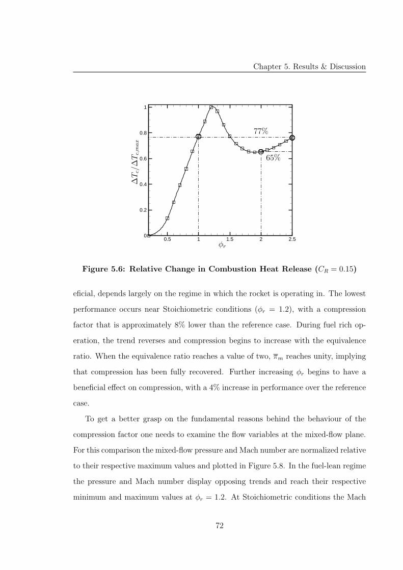
Chapter 5. Results & Discussion
0.5 1 1.5 2 2.50
0.2
0.4
0.6
0.8
1
φr
∆T
c/∆
Tc,
max
77%
65%
Figure 5.6: Relative Change in Combustion Heat Release (CR = 0.15)
eficial, depends largely on the regime in which the rocket is operating in. The lowest
performance occurs near Stoichiometric conditions (φr = 1.2), with a compression
factor that is approximately 8% lower than the reference case. During fuel rich op-
eration, the trend reverses and compression begins to increase with the equivalence
ratio. When the equivalence ratio reaches a value of two, πm reaches unity, implying
that compression has been fully recovered. Further increasing φr begins to have a
beneficial effect on compression, with a 4% increase in performance over the reference
case.
To get a better grasp on the fundamental reasons behind the behaviour of the
compression factor one needs to examine the flow variables at the mixed-flow plane.
For this comparison the mixed-flow pressure and Mach number are normalized relative
to their respective maximum values and plotted in Figure 5.8. In the fuel-lean regime
the pressure and Mach number display opposing trends and reach their respective
minimum and maximum values at φr = 1.2. At Stoichiometric conditions the Mach
72
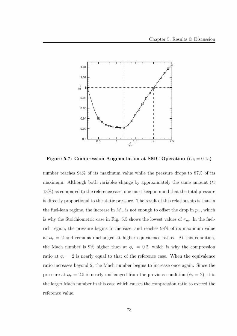
Chapter 5. Results & Discussion
0.5 1 1.5 2 2.50.9
0.92
0.94
0.96
0.98
1
1.02
1.04
φr
πm
Figure 5.7: Compression Augmentation at SMC Operation (CR = 0.15)
number reaches 94% of its maximum value while the pressure drops to 87% of its
maximum. Although both variables change by approximately the same amount (≈
13%) as compared to the reference case, one must keep in mind that the total pressure
is directly proportional to the static pressure. The result of this relationship is that in
the fuel-lean regime, the increase in Mm is not enough to offset the drop in pm, which
is why the Stoichiometric case in Fig. 5.5 shows the lowest values of πm. In the fuel-
rich region, the pressure begins to increase, and reaches 98% of its maximum value
at φr = 2 and remains unchanged at higher equivalence ratios. At this condition,
the Mach number is 9% higher than at φr = 0.2, which is why the compression
ratio at φr = 2 is nearly equal to that of the reference case. When the equivalence
ratio increases beyond 2, the Mach number begins to increase once again. Since the
pressure at φr = 2.5 is nearly unchanged from the previous condition (φr = 2), it is
the larger Mach number in this case which causes the compression ratio to exceed the
reference value.
73
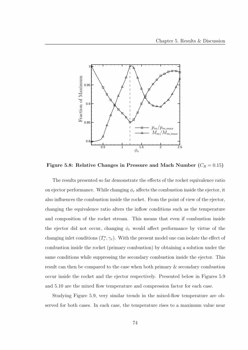
Chapter 5. Results & Discussion
0.5 1 1.5 2 2.5
0.8
0.85
0.9
0.95
1
φr
Fra
ctio
nof
Max
imum
pm/pm,max
Mm/Mm,max
Figure 5.8: Relative Changes in Pressure and Mach Number (CR = 0.15)
The results presented so far demonstrate the effects of the rocket equivalence ratio
on ejector performance. While changing φr affects the combustion inside the ejector, it
also influences the combustion inside the rocket. From the point of view of the ejector,
changing the equivalence ratio alters the inflow conditions such as the temperature
and composition of the rocket stream. This means that even if combustion inside
the ejector did not occur, changing φr would affect performance by virtue of the
changing inlet conditions (T or , γr). With the present model one can isolate the effect of
combustion inside the rocket (primary combustion) by obtaining a solution under the
same conditions while suppressing the secondary combustion inside the ejector. This
result can then be compared to the case when both primary & secondary combustion
occur inside the rocket and the ejector respectively. Presented below in Figures 5.9
and 5.10 are the mixed flow temperature and compression factor for each case.
Studying Figure 5.9, very similar trends in the mixed-flow temperature are ob-
served for both cases. In each case, the temperature rises to a maximum value near
74
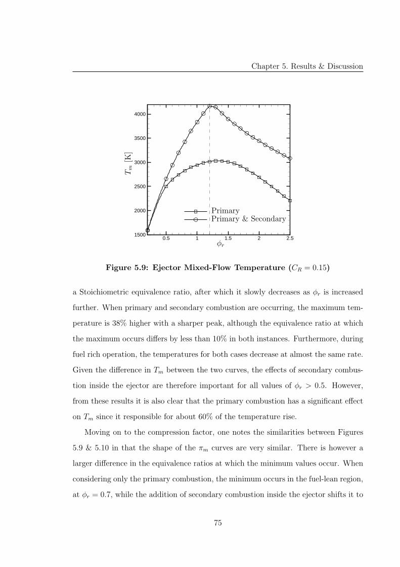
Chapter 5. Results & Discussion
0.5 1 1.5 2 2.51500
2000
2500
3000
3500
4000
φr
Tm
[K]
PrimaryPrimary & Secondary
Figure 5.9: Ejector Mixed-Flow Temperature (CR = 0.15)
a Stoichiometric equivalence ratio, after which it slowly decreases as φr is increased
further. When primary and secondary combustion are occurring, the maximum tem-
perature is 38% higher with a sharper peak, although the equivalence ratio at which
the maximum occurs differs by less than 10% in both instances. Furthermore, during
fuel rich operation, the temperatures for both cases decrease at almost the same rate.
Given the difference in Tm between the two curves, the effects of secondary combus-
tion inside the ejector are therefore important for all values of φr > 0.5. However,
from these results it is also clear that the primary combustion has a significant effect
on Tm since it responsible for about 60% of the temperature rise.
Moving on to the compression factor, one notes the similarities between Figures
5.9 & 5.10 in that the shape of the πm curves are very similar. There is however a
larger difference in the equivalence ratios at which the minimum values occur. When
considering only the primary combustion, the minimum occurs in the fuel-lean region,
at φr = 0.7, while the addition of secondary combustion inside the ejector shifts it to
75
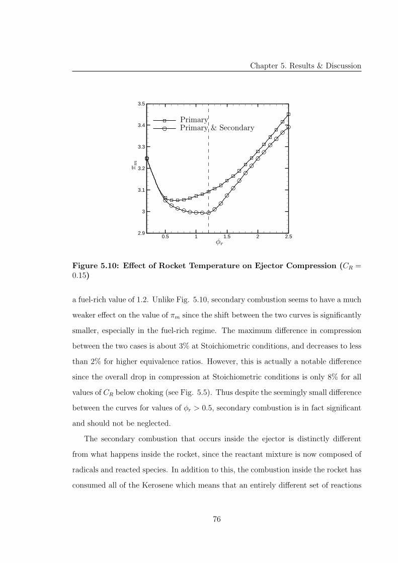
Chapter 5. Results & Discussion
0.5 1 1.5 2 2.52.9
3
3.1
3.2
3.3
3.4
3.5
φr
πm
PrimaryPrimary & Secondary
Figure 5.10: Effect of Rocket Temperature on Ejector Compression (CR =0.15)
a fuel-rich value of 1.2. Unlike Fig. 5.10, secondary combustion seems to have a much
weaker effect on the value of πm since the shift between the two curves is significantly
smaller, especially in the fuel-rich regime. The maximum difference in compression
between the two cases is about 3% at Stoichiometric conditions, and decreases to less
than 2% for higher equivalence ratios. However, this is actually a notable difference
since the overall drop in compression at Stoichiometric conditions is only 8% for all
values of CR below choking (see Fig. 5.5). Thus despite the seemingly small difference
between the curves for values of φr > 0.5, secondary combustion is in fact significant
and should not be neglected.
The secondary combustion that occurs inside the ejector is distinctly different
from what happens inside the rocket, since the reactant mixture is now composed of
radicals and reacted species. In addition to this, the combustion inside the rocket has
consumed all of the Kerosene which means that an entirely different set of reactions
76
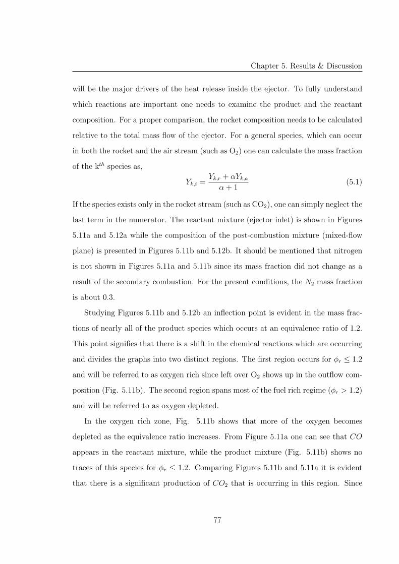
Chapter 5. Results & Discussion
will be the major drivers of the heat release inside the ejector. To fully understand
which reactions are important one needs to examine the product and the reactant
composition. For a proper comparison, the rocket composition needs to be calculated
relative to the total mass flow of the ejector. For a general species, which can occur
in both the rocket and the air stream (such as O2) one can calculate the mass fraction
of the kth species as,
Yk,i =Yk,r + αYk,a
α+ 1(5.1)
If the species exists only in the rocket stream (such as CO2), one can simply neglect the
last term in the numerator. The reactant mixture (ejector inlet) is shown in Figures
5.11a and 5.12a while the composition of the post-combustion mixture (mixed-flow
plane) is presented in Figures 5.11b and 5.12b. It should be mentioned that nitrogen
is not shown in Figures 5.11a and 5.11b since its mass fraction did not change as a
result of the secondary combustion. For the present conditions, the N2 mass fraction
is about 0.3.
Studying Figures 5.11b and 5.12b an inflection point is evident in the mass frac-
tions of nearly all of the product species which occurs at an equivalence ratio of 1.2.
This point signifies that there is a shift in the chemical reactions which are occurring
and divides the graphs into two distinct regions. The first region occurs for φr ≤ 1.2
and will be referred to as oxygen rich since left over O2 shows up in the outflow com-
position (Fig. 5.11b). The second region spans most of the fuel rich regime (φr > 1.2)
and will be referred to as oxygen depleted.
In the oxygen rich zone, Fig. 5.11b shows that more of the oxygen becomes
depleted as the equivalence ratio increases. From Figure 5.11a one can see that CO
appears in the reactant mixture, while the product mixture (Fig. 5.11b) shows no
traces of this species for φr ≤ 1.2. Comparing Figures 5.11b and 5.11a it is evident
that there is a significant production of CO2 that is occurring in this region. Since
77

Chapter 5. Results & Discussion
0.5 1 1.5 2 2.50
0.1
0.2
0.3
0.4
0.5
φr
YCO2
COH2OO2
(a) Inlet
0.5 1 1.5 2 2.50
0.1
0.2
0.3
0.4
0.5
φr
Y
CO2
COH2OO2
(b) Post-Combustion
Figure 5.11: Ejector Composition - Major Species (CR = 0.15)
78
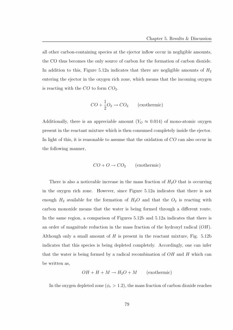
Chapter 5. Results & Discussion
all other carbon-containing species at the ejector inflow occur in negligible amounts,
the CO thus becomes the only source of carbon for the formation of carbon dioxide.
In addition to this, Figure 5.12a indicates that there are negligible amounts of H2
entering the ejector in the oxygen rich zone, which means that the incoming oxygen
is reacting with the CO to form CO2.
CO +1
2O2 → CO2 (exothermic)
Additionally, there is an appreciable amount (YO ≈ 0.014) of mono-atomic oxygen
present in the reactant mixture which is then consumed completely inside the ejector.
In light of this, it is reasonable to assume that the oxidation of CO can also occur in
the following manner,
CO +O → CO2 (exothermic)
There is also a noticeable increase in the mass fraction of H2O that is occurring
in the oxygen rich zone. However, since Figure 5.12a indicates that there is not
enough H2 available for the formation of H2O and that the O2 is reacting with
carbon monoxide means that the water is being formed through a different route.
In the same region, a comparison of Figures 5.12b and 5.12a indicates that there is
an order of magnitude reduction in the mass fraction of the hydroxyl radical (OH).
Although only a small amount of H is present in the reactant mixture, Fig. 5.12b
indicates that this species is being depleted completely. Accordingly, one can infer
that the water is being formed by a radical recombination of OH and H which can
be written as,
OH +H +M → H2O +M (exothermic)
In the oxygen depleted zone (φr > 1.2), the mass fraction of carbon dioxide reaches
79
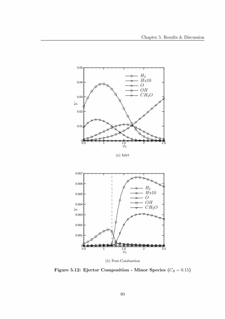
Chapter 5. Results & Discussion
0.5 1 1.5 2 2.50
0.01
0.02
0.03
0.04
0.05
φr
YH2
Hx10OOHCH2O
(a) Inlet
0.5 1 1.5 2 2.50
0.001
0.002
0.003
0.004
0.005
0.006
0.007
φr
Y
H2
Hx10OOHCH2O
(b) Post-Combustion
Figure 5.12: Ejector Composition - Minor Species (CR = 0.15)
80
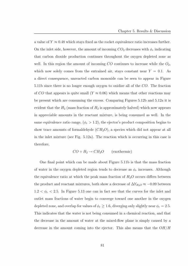
Chapter 5. Results & Discussion
a value of Y ≈ 0.48 which stays fixed as the rocket equivalence ratio increases further.
On the inlet side, however, the amount of incoming CO2 decreases with φr indicating
that carbon dioxide production continues throughout the oxygen depleted zone as
well. In this region the amount of incoming CO continues to increase while the O2,
which now solely comes from the entrained air, stays constant near Y = 0.1. As
a direct consequence, unreacted carbon monoxide can be seen to appear in Figure
5.11b since there is no longer enough oxygen to oxidize all of the CO. The fraction
of CO that appears is quite small (Y ≈ 0.06) which means that other reactions may
be present which are consuming the excess. Comparing Figures 5.12b and 5.12a it is
evident that the H2 (mass fraction of H2 is approximately halved) which now appears
in appreciable amounts in the reactant mixture, is being consumed as well. In the
same equivalence ratio range, (φr > 1.2), the ejector’s product composition begins to
show trace amounts of formaldehyde (CH2O), a species which did not appear at all
in the inlet mixture (see Fig. 5.12a). The reaction which is occurring in this case is
therefore,
CO +H2 → CH2O (exothermic)
One final point which can be made about Figure 5.11b is that the mass fraction
of water in the oxygen depleted region tends to decrease as φr increases. Although
the equivalence ratio at which the peak mass fraction of H2O occurs differs between
the product and reactant mixtures, both show a decrease of ∆YH2O ≈ −0.09 between
1.2 < φr < 2.5. In Figure 5.13 one can in fact see that the curves for the inlet and
outlet mass fractions of water begin to converge toward one another in the oxygen
depleted zone, and overlap for values of φr ≥ 1.6, diverging only slightly near φr = 2.5.
This indicates that the water is not being consumed in a chemical reaction, and that
the decrease in the amount of water at the mixed-flow plane is simply caused by a
decrease in the amount coming into the ejector. This also means that the OH/H
81
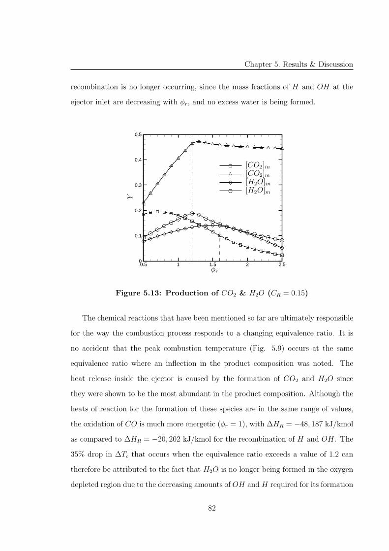
Chapter 5. Results & Discussion
recombination is no longer occurring, since the mass fractions of H and OH at the
ejector inlet are decreasing with φr, and no excess water is being formed.
0.5 1 1.5 2 2.50
0.1
0.2
0.3
0.4
0.5
φr
Y
[CO2]in[CO2]m[H2O]in[H2O]m
Figure 5.13: Production of CO2 & H2O (CR = 0.15)
The chemical reactions that have been mentioned so far are ultimately responsible
for the way the combustion process responds to a changing equivalence ratio. It is
no accident that the peak combustion temperature (Fig. 5.9) occurs at the same
equivalence ratio where an inflection in the product composition was noted. The
heat release inside the ejector is caused by the formation of CO2 and H2O since
they were shown to be the most abundant in the product composition. Although the
heats of reaction for the formation of these species are in the same range of values,
the oxidation of CO is much more energetic (φr = 1), with ∆HR = −48, 187 kJ/kmol
as compared to ∆HR = −20, 202 kJ/kmol for the recombination of H and OH. The
35% drop in ∆Tc that occurs when the equivalence ratio exceeds a value of 1.2 can
therefore be attributed to the fact that H2O is no longer being formed in the oxygen
depleted region due to the decreasing amounts of OH andH required for its formation
82
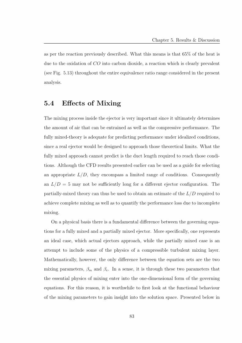
Chapter 5. Results & Discussion
as per the reaction previously described. What this means is that 65% of the heat is
due to the oxidation of CO into carbon dioxide, a reaction which is clearly prevalent
(see Fig. 5.13) throughout the entire equivalence ratio range considered in the present
analysis.
5.4 Effects of Mixing
The mixing process inside the ejector is very important since it ultimately determines
the amount of air that can be entrained as well as the compressive performance. The
fully mixed-theory is adequate for predicting performance under idealized conditions,
since a real ejector would be designed to approach those theoretical limits. What the
fully mixed approach cannot predict is the duct length required to reach those condi-
tions. Although the CFD results presented earlier can be used as a guide for selecting
an appropriate L/D, they encompass a limited range of conditions. Consequently
an L/D = 5 may not be sufficiently long for a different ejector configuration. The
partially-mixed theory can thus be used to obtain an estimate of the L/D required to
achieve complete mixing as well as to quantify the performance loss due to incomplete
mixing.
On a physical basis there is a fundamental difference between the governing equa-
tions for a fully mixed and a partially mixed ejector. More specifically, one represents
an ideal case, which actual ejectors approach, while the partially mixed case is an
attempt to include some of the physics of a compressible turbulent mixing layer.
Mathematically, however, the only difference between the equation sets are the two
mixing parameters, βm and βe. In a sense, it is through these two parameters that
the essential physics of mixing enter into the one-dimensional form of the governing
equations. For this reason, it is worthwhile to first look at the functional behaviour
of the mixing parameters to gain insight into the solution space. Presented below in
83
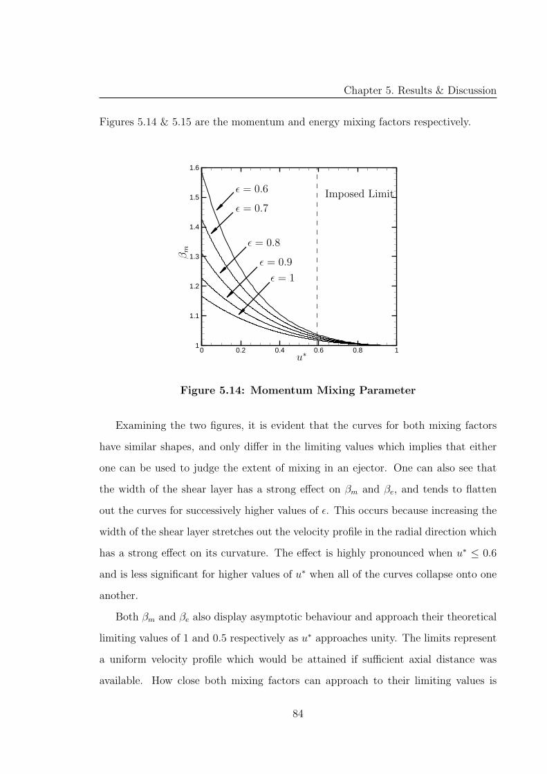
Chapter 5. Results & Discussion
Figures 5.14 & 5.15 are the momentum and energy mixing factors respectively.
0 0.2 0.4 0.6 0.8 11
1.1
1.2
1.3
1.4
1.5
1.6
u∗
βm
ǫ = 0.6
ǫ = 0.7
ǫ = 0.8
ǫ = 0.9
ǫ = 1
Imposed Limit
Figure 5.14: Momentum Mixing Parameter
Examining the two figures, it is evident that the curves for both mixing factors
have similar shapes, and only differ in the limiting values which implies that either
one can be used to judge the extent of mixing in an ejector. One can also see that
the width of the shear layer has a strong effect on βm and βe, and tends to flatten
out the curves for successively higher values of ǫ. This occurs because increasing the
width of the shear layer stretches out the velocity profile in the radial direction which
has a strong effect on its curvature. The effect is highly pronounced when u∗ ≤ 0.6
and is less significant for higher values of u∗ when all of the curves collapse onto one
another.
Both βm and βe also display asymptotic behaviour and approach their theoretical
limiting values of 1 and 0.5 respectively as u∗ approaches unity. The limits represent
a uniform velocity profile which would be attained if sufficient axial distance was
available. How close both mixing factors can approach to their limiting values is
84
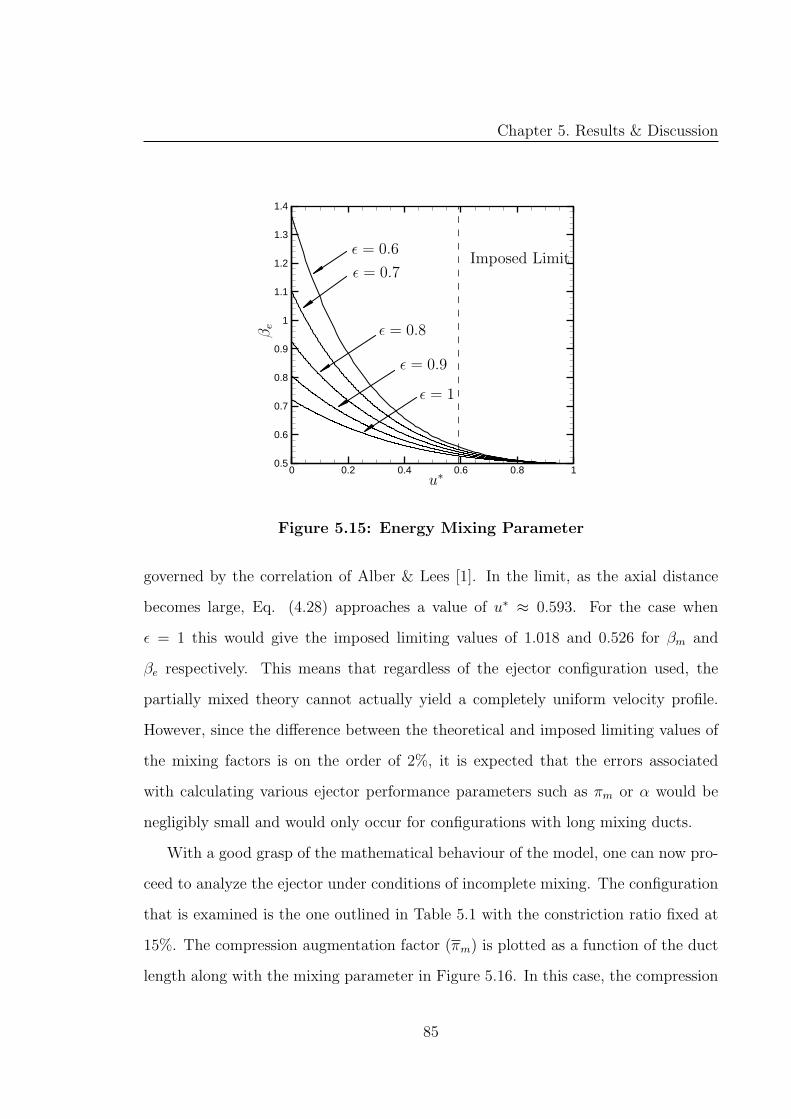
Chapter 5. Results & Discussion
0 0.2 0.4 0.6 0.8 10.5
0.6
0.7
0.8
0.9
1
1.1
1.2
1.3
1.4
u∗
βe
ǫ = 0.6
ǫ = 0.7
ǫ = 0.8
ǫ = 0.9
ǫ = 1
Imposed Limit
Figure 5.15: Energy Mixing Parameter
governed by the correlation of Alber & Lees [1]. In the limit, as the axial distance
becomes large, Eq. (4.28) approaches a value of u∗ ≈ 0.593. For the case when
ǫ = 1 this would give the imposed limiting values of 1.018 and 0.526 for βm and
βe respectively. This means that regardless of the ejector configuration used, the
partially mixed theory cannot actually yield a completely uniform velocity profile.
However, since the difference between the theoretical and imposed limiting values of
the mixing factors is on the order of 2%, it is expected that the errors associated
with calculating various ejector performance parameters such as πm or α would be
negligibly small and would only occur for configurations with long mixing ducts.
With a good grasp of the mathematical behaviour of the model, one can now pro-
ceed to analyze the ejector under conditions of incomplete mixing. The configuration
that is examined is the one outlined in Table 5.1 with the constriction ratio fixed at
15%. The compression augmentation factor (πm) is plotted as a function of the duct
length along with the mixing parameter in Figure 5.16. In this case, the compression
85
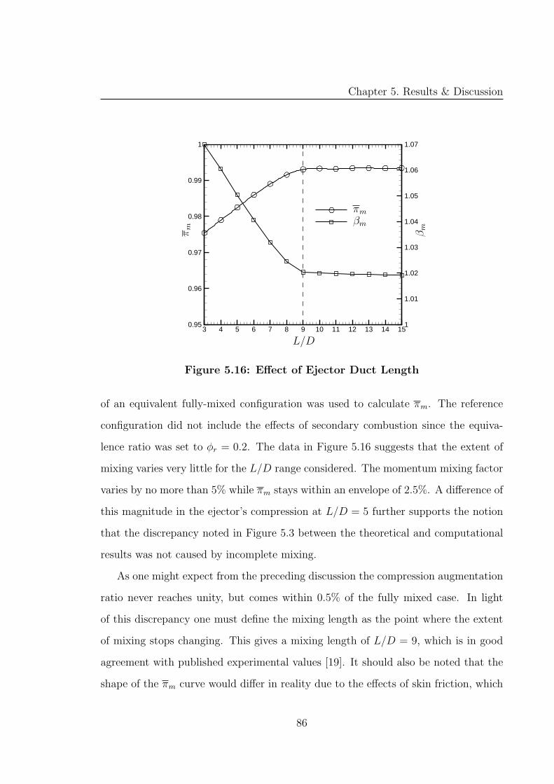
Chapter 5. Results & Discussion
3 4 5 6 7 8 9 10 11 12 13 14 150.95
0.96
0.97
0.98
0.99
1
1
1.01
1.02
1.03
1.04
1.05
1.06
1.07
L/D
πm
πm
βm
βm
Figure 5.16: Effect of Ejector Duct Length
of an equivalent fully-mixed configuration was used to calculate πm. The reference
configuration did not include the effects of secondary combustion since the equiva-
lence ratio was set to φr = 0.2. The data in Figure 5.16 suggests that the extent of
mixing varies very little for the L/D range considered. The momentum mixing factor
varies by no more than 5% while πm stays within an envelope of 2.5%. A difference of
this magnitude in the ejector’s compression at L/D = 5 further supports the notion
that the discrepancy noted in Figure 5.3 between the theoretical and computational
results was not caused by incomplete mixing.
As one might expect from the preceding discussion the compression augmentation
ratio never reaches unity, but comes within 0.5% of the fully mixed case. In light
of this discrepancy one must define the mixing length as the point where the extent
of mixing stops changing. This gives a mixing length of L/D = 9, which is in good
agreement with published experimental values [19]. It should also be noted that the
shape of the πm curve would differ in reality due to the effects of skin friction, which
86
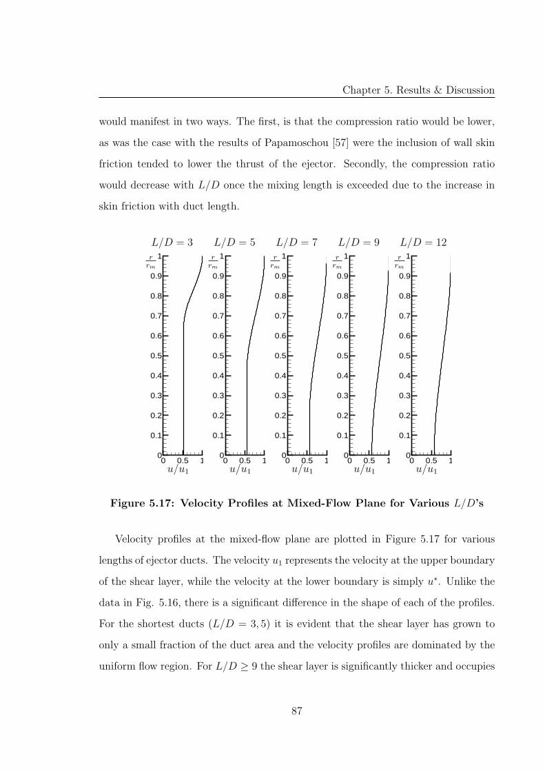
Chapter 5. Results & Discussion
would manifest in two ways. The first, is that the compression ratio would be lower,
as was the case with the results of Papamoschou [57] were the inclusion of wall skin
friction tended to lower the thrust of the ejector. Secondly, the compression ratio
would decrease with L/D once the mixing length is exceeded due to the increase in
skin friction with duct length.
0 0.5 10
0.1
0.2
0.3
0.4
0.5
0.6
0.7
0.8
0.9
1
0 0.5 10
0.1
0.2
0.3
0.4
0.5
0.6
0.7
0.8
0.9
1
0 0.5 10
0.1
0.2
0.3
0.4
0.5
0.6
0.7
0.8
0.9
1
0 0.5 10
0.1
0.2
0.3
0.4
0.5
0.6
0.7
0.8
0.9
1
0 0.5 10
0.1
0.2
0.3
0.4
0.5
0.6
0.7
0.8
0.9
1rrm
rrm
rrm
rrm
rrm
u/u1u/u1u/u1u/u1u/u1
L/D = 3 L/D = 5 L/D = 7 L/D = 9 L/D = 12
Figure 5.17: Velocity Profiles at Mixed-Flow Plane for Various L/D’s
Velocity profiles at the mixed-flow plane are plotted in Figure 5.17 for various
lengths of ejector ducts. The velocity u1 represents the velocity at the upper boundary
of the shear layer, while the velocity at the lower boundary is simply u∗. Unlike the
data in Fig. 5.16, there is a significant difference in the shape of each of the profiles.
For the shortest ducts (L/D = 3, 5) it is evident that the shear layer has grown to
only a small fraction of the duct area and the velocity profiles are dominated by the
uniform flow region. For L/D ≥ 9 the shear layer is significantly thicker and occupies
87
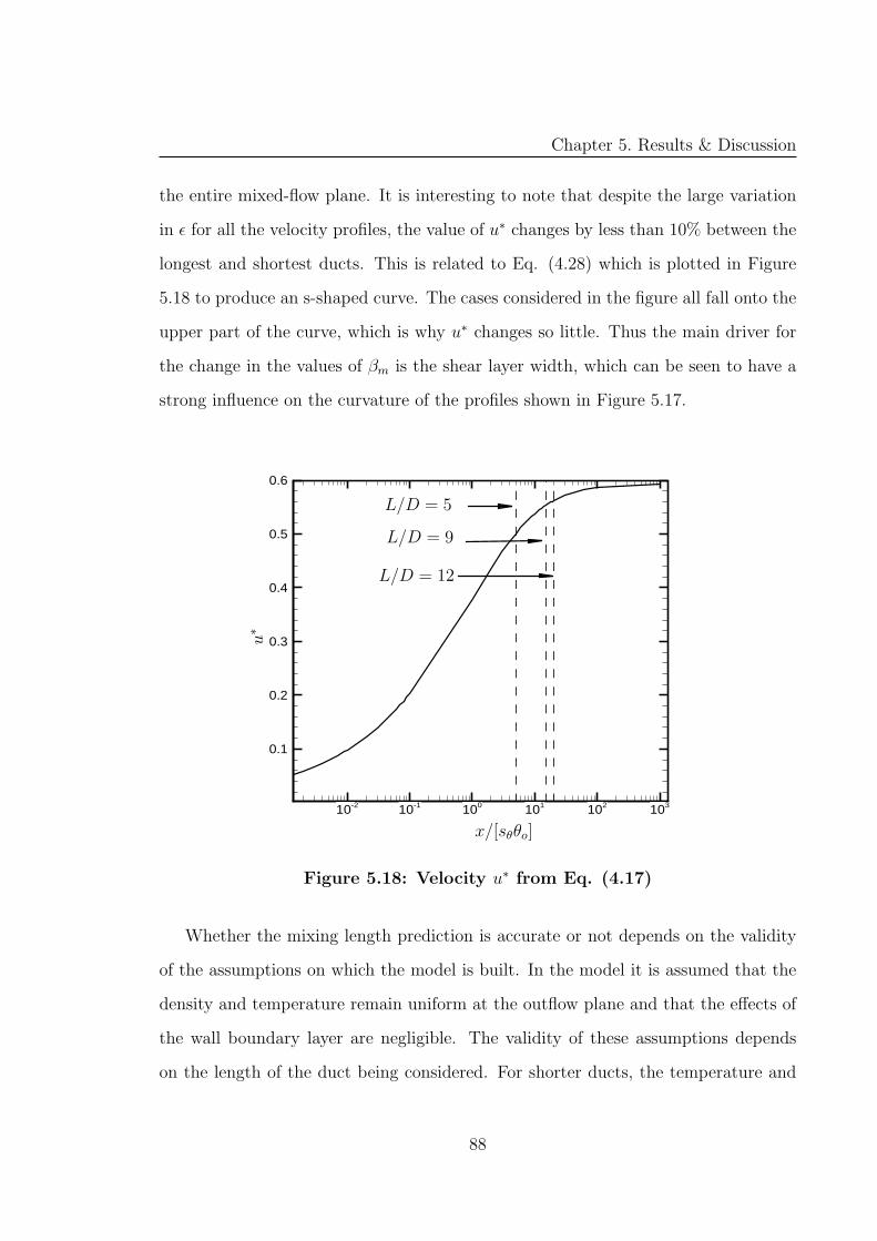
Chapter 5. Results & Discussion
the entire mixed-flow plane. It is interesting to note that despite the large variation
in ǫ for all the velocity profiles, the value of u∗ changes by less than 10% between the
longest and shortest ducts. This is related to Eq. (4.28) which is plotted in Figure
5.18 to produce an s-shaped curve. The cases considered in the figure all fall onto the
upper part of the curve, which is why u∗ changes so little. Thus the main driver for
the change in the values of βm is the shear layer width, which can be seen to have a
strong influence on the curvature of the profiles shown in Figure 5.17.
10-2 10-1 100 101 102 103
0.1
0.2
0.3
0.4
0.5
0.6
u∗
x/[sθθo]
L/D = 5
L/D = 9
L/D = 12
Figure 5.18: Velocity u∗ from Eq. (4.17)
Whether the mixing length prediction is accurate or not depends on the validity
of the assumptions on which the model is built. In the model it is assumed that the
density and temperature remain uniform at the outflow plane and that the effects of
the wall boundary layer are negligible. The validity of these assumptions depends
on the length of the duct being considered. For shorter ducts, the temperature and
88
Chapter 5. Results & Discussion
density profiles may no longer be uniform while the effects of the wall boundary layer
would become important for longer ducts. Since the temperature and density profiles
in the CFD results were uniform for L/D = 5, it is therefore reasonable to assume
that those effects would not alter the prediction of the model. The wall boundary
layer, on the other hand, may be fairly thick for L/D = 9 and although it would
increase the mixing factor, the extent of the mixing would remain unchanged. In
addition to these considerations, one must also keep in mind that the model uses a
correlation for a planar shear layer to estimate the mixing extent in an axisymmetric
case. Since axisymmetric shear layers tend to spread out faster [64], the mixing length
predicted by the model is most likely a conservative estimate.
5.5 Thrust Augmentation
The thrust of an ejector depends not only on how effectively it compresses the incom-
ing air but also on how much air it entrains. The results presented so far have only
dealt with the compression ratio, since α was held fixed. To quantify the effects of
CR and φr in a more complete manner, one needs to look at the how well the ejector
augments thrust. The analysis will therefore consider a fully-mixed ejector under
SMC conditions while using the case when combustion does not occur (φr = 0.2) as
a reference. The ejector configuration is modified to include a rocket that is repre-
sentative of an Atlas E/F first stage (Rocketdyne MA-3 engine), with the pertinent
parameters shown in Table 5.4.
The ejector configuration used for thrust calculations is shown in Figure 5.19 and
is fitted with a diverging propelling nozzle since the mixed-flow Mach number is fixed
at unity for all cases. The flow entering the nozzle at plane m is assumed to expand
isentropically to atmospheric pressure (p∞) by the time it reaches plane e. Given
that the pressures at either end of the nozzle are specified (pm, pe), and pm can vary
89
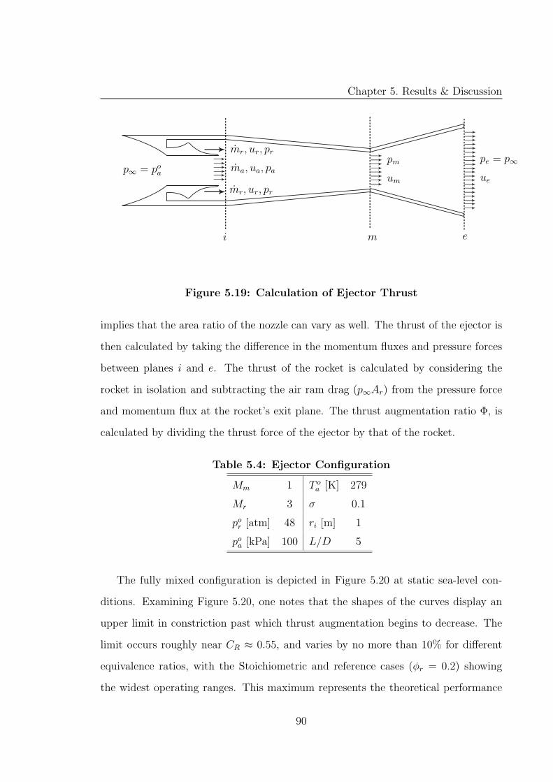
Chapter 5. Results & Discussion
mr, ur, pr
mr, ur, pr
ma, ua, pa
pm
um
pe = p∞
ue
p∞ = poa
i m e
Figure 5.19: Calculation of Ejector Thrust
implies that the area ratio of the nozzle can vary as well. The thrust of the ejector is
then calculated by taking the difference in the momentum fluxes and pressure forces
between planes i and e. The thrust of the rocket is calculated by considering the
rocket in isolation and subtracting the air ram drag (p∞Ar) from the pressure force
and momentum flux at the rocket’s exit plane. The thrust augmentation ratio Φ, is
calculated by dividing the thrust force of the ejector by that of the rocket.
Table 5.4: Ejector Configuration
Mm 1 T oa [K] 279
Mr 3 σ 0.1
por [atm] 48 ri [m] 1
poa [kPa] 100 L/D 5
The fully mixed configuration is depicted in Figure 5.20 at static sea-level con-
ditions. Examining Figure 5.20, one notes that the shapes of the curves display an
upper limit in constriction past which thrust augmentation begins to decrease. The
limit occurs roughly near CR ≈ 0.55, and varies by no more than 10% for different
equivalence ratios, with the Stoichiometric and reference cases (φr = 0.2) showing
the widest operating ranges. This maximum represents the theoretical performance
90
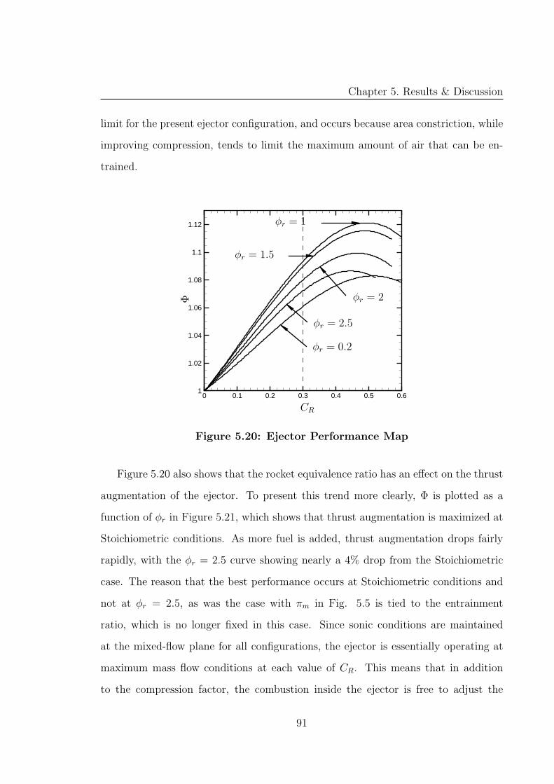
Chapter 5. Results & Discussion
limit for the present ejector configuration, and occurs because area constriction, while
improving compression, tends to limit the maximum amount of air that can be en-
trained.
0 0.1 0.2 0.3 0.4 0.5 0.61
1.02
1.04
1.06
1.08
1.1
1.12
CR
Φ
φr = 0.2
φr = 1
φr = 1.5
φr = 2
φr = 2.5
Figure 5.20: Ejector Performance Map
Figure 5.20 also shows that the rocket equivalence ratio has an effect on the thrust
augmentation of the ejector. To present this trend more clearly, Φ is plotted as a
function of φr in Figure 5.21, which shows that thrust augmentation is maximized at
Stoichiometric conditions. As more fuel is added, thrust augmentation drops fairly
rapidly, with the φr = 2.5 curve showing nearly a 4% drop from the Stoichiometric
case. The reason that the best performance occurs at Stoichiometric conditions and
not at φr = 2.5, as was the case with πm in Fig. 5.5 is tied to the entrainment
ratio, which is no longer fixed in this case. Since sonic conditions are maintained
at the mixed-flow plane for all configurations, the ejector is essentially operating at
maximum mass flow conditions at each value of CR. This means that in addition
to the compression factor, the combustion inside the ejector is free to adjust the
91
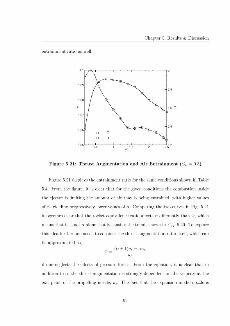
Chapter 5. Results & Discussion
entrainment ratio as well.
0.5 1 1.5 2 2.51.05
1.06
1.07
1.08
1.09
1.1
1.2
1.4
1.6
1.8
2
φr
Φ
Φ
α
α
Figure 5.21: Thrust Augmentation and Air Entrainment (CR = 0.3)
Figure 5.21 displays the entrainment ratio for the same conditions shown in Table
5.4. From the figure, it is clear that for the given conditions the combustion inside
the ejector is limiting the amount of air that is being entrained, with higher values
of φr yielding progressively lower values of α. Comparing the two curves in Fig. 5.21
it becomes clear that the rocket equivalence ratio affects α differently than Φ, which
means that it is not α alone that is causing the trends shown in Fig. 5.20. To explore
this idea further one needs to consider the thrust augmentation ratio itself, which can
be approximated as,
Φ =(α+ 1)ue − αua
ur
if one neglects the effects of pressure forces. From the equation, it is clear that in
addition to α, the thrust augmentation is strongly dependent on the velocity at the
exit plane of the propelling nozzle, ue. The fact that the expansion in the nozzle is
92
Chapter 5. Results & Discussion
isentropic implies that ue is proportional to the mixed-flow velocity, um. Referring
back to Figure 5.8 one notes that the maximum mixed-flow Mach number occurred
near Stoichiometric conditions (φr = 1.2 to be precise). Combining this with the fact
that the maximum temperature occurred at the same value of φr yields a mixed-flow
velocity that is nearly double that of the reference case. On the other hand, Figure
5.21 shows that 26% more air is entrained at reference conditions as compared to the
Stoichiometric case. The net effect of the two is a higher thrust augmentation ratio,
since the nearly two-fold increase in um offsets the 26% drop in α. At higher equiva-
lence ratios, both the mixed-flow velocity and the entrainment ratio are diminished,
thus causing the lower levels of thrust present at those conditions.
93

Chapter 6
Conclusions
A theoretical treatment for a constricted ejector has been presented. The bulk of the
theory relied on the assumption of complete mixing and used an equilibrium calcula-
tion procedure to analyze the SMC operating regime. For a non-reacting case, modifi-
cations to the preceding theory were introduced to account for incomplete mixing and
its effects on overall performance. In either case, a wall pressure distribution needed
to be assumed to close the system of equations. Several options for this pressure
distribution were presented, namely two analytical functions (linear & polynomial)
as well as wall pressures extracted directly from CFD simulations.
Other than the inlet and exit pressures, the polynomial pressure distribution re-
quired that the minimum rocket pressure, pmin be specified. Two methods for calcu-
lating this quantity were presented, one which made use of a Riemann solver and an-
other which made use of a control volume (CV method) formulation. Both techniques
predicted very similar values of pmin because of the common assumptions (isentropic
flow, no mixing) on which the methods were based. In addition, the analytical so-
lutions for pmin were 60-70% larger than the CFD prediction due to non-isentropic
effects as well as the highly two-dimensional flow in the computational case.
To evaluate which pressure distribution was the most appropriate in terms of
94
Chapter 6. Conclusions
accuracy, solutions under non-reacting, fully mixed conditions were obtained for the
ejector’s compression (πm) and compression augmentation (πm) factors. Overall, the
trends for ejector compression that were obtained were very close to the CFD results,
although the analytical values of πm were about 30-40% higher, with turbulent and
viscous effects being identified as the major causes. Within the theoretical solutions,
it was found that the polynomial pressure distribution was the best approximation
for quantifying Fp,x since the results it gave for πm and πm were very close to those
obtained when the CFD wall pressures were used.
Further analysis of the fully mixed ejector was performed under SMC conditions
by varying the equivalence ratio of the rocket in the range 0.2 < φr < 2.5. Op-
eration in this mode caused significant thermal choking for φr ≥ 1 which reduced
the allowable range of CR by 14% in the worst case, and was directly related to the
combustion temperature rise inside the ejector. The combustion also affected the
ejector’s compression ratio in a manner which depended on the equivalence ratio at
which the rocket was operating. At Stoichiometric conditions, there was an 8% drop
in πm which was caused by a lower mixed-flow pressure, while the highest compres-
sion ratio occurred at an equivalence ratio of 2.5 due to an increased Mach number.
For all values of φr > 0.5 the effects of the secondary combustion were significant
and were responsible for about 40% of the changes noted in the ejector’s mixed-flow
temperature and compression ratio.
Examination of the ejector’s post-combustion mixture revealed the existence of
an inflection point in the mass fractions of nearly all of the product species which
occurred at φr = 1.2 and effectively split the equivalence ratio range into two zones.
The oxidation of CO and the recombination of H and OH where shown to be the
reactions primarily responsible for the heat release inside the ejector. While the
Carbon Monoxide reaction persisted throughout the entire equivalence ratio range,
the radical recombination was mainly active in the oxygen rich zone, and is in fact
95
Chapter 6. Conclusions
what caused the inflection point and the subsequent drop in the heat release at higher
equivalence ratios.
The partially mixed theory was used to estimate the mixing length required to
achieve fully mixed conditions as well as to quantify the drop in compression caused
by incomplete mixing. For long mixing ducts, it was shown that the model was not
able to produce a completely uniform velocity profile due to the correlation used to
define u∗. Although a mixing duct with an L/D = 5 yielded a flow that was 95%
mixed with a compression ratio that was only 2.5% lower than the fully mixed value,
a limit in the mixing extent was not reached until an L/D = 9. Furthermore, for
the L/D range considered, the drop in πm due to incomplete mixing never exceeded
2.5%, further proving that incomplete mixing was not the cause of the discrepancy
between the theoretical and the computational results.
The thrust augmenting performance of the ejector was investigated under fully
mixed conditions. The case when secondary combustion was absent at φr = 0.2 was
used as a reference throughout. The results showed an upper limit in thrust augmen-
tation near CR ≈ 0.55 past which Φ decreased. Maximum thrust augmentation was
achieved at φr = 1, while operation in the fuel rich regime caused a 4% drop in Φ at
an equivalence ratio of 2.5. This occurred because compared to the reference case,
there was a two-fold increase in the mixed-flow velocity at Stoichiometric conditions
while α decreased by only 26%.
96
Chapter 6. Conclusions
6.1 Future Work
In light of the results reported in this study there are several routes which any research
that follows can take. The fully-mixed theory that was outlined in this work is
complete and should not be developed further. The best course of action would be to
use the theory to obtain performance data under operating conditions not covered in
the present work. An example of this would be to look at the DAB mode of operation
as well as to find the optimum operating parameters for this mode. Alternatively one
can use the fully-mixed theory in an optimization routine of some sort to generate
one or more optimized ejector configurations.
The partially-mixed theory, on the other hand, should be extended to include the
effects of non-uniform temperature and density profiles for instance. Although not
crucial, a correlation for u∗ which is better suited to the present application should
be found to ensure that a fully mixed case can be reached under the right operating
conditions. One can also modify the theory slightly to account for the effect of
wall skin friction, which would provide a more realistic prediction of the ejector’s
performance.
The Riemann approach that was introduced also warrants further investigation,
to see if it alone can be used to predict the ejector’s performance. Since the Riemann
approach essentially solves the ejector flowfield in a piece-wise manner, it is therefore
well suited for use in a more complex, differential ejector model, similar to the one
suggested by Papamoschou [57]. The advantage of using the Riemann solver in this
manner would be that one would no longer have to consider an ejector where the
pressures of the two streams are matched.
97
Bibliography
[1] Alber, I. E. and Lees, L., “Integral Theory for Supersonic Turbulent Base Flows,”
AIAA Journal , Vol. 6, No. 7, 1968.
[2] Alperin, M. and Wu, J. J., “Thrust Augmenting Ejectors, Part I,” AIAA Journal ,
Vol. 21, No. 10, 1983.
[3] Anderson, J. D., Fundamentals of Aerodynamics , McGraw Hill, 3rd ed., 2001.
[4] Anderson, J. D., Modern Compressible Flow , McGraw Hill, 3rd ed., 2002.
[5] Anderson, J. D., Computational Fluid Dynamics , McGraw Hill, 1995.
[6] Aoki, S., Lee, J., and Masuya, G., “Aerodynamic Experiment on an Ejector-Jet,”
Journal of Propulsion and Power , Vol. 21, No. 3, 2005.
[7] Bartosiewicz, Y., Aidoun, Z., Desevaux, P., and Mercadier, Y., “Numerical and
Experimental Investigations on Supersonic Ejectors,” Int. Journal of Heat and
Fluid Flow , Vol. 26, 2006, pp. 56–70.
[8] Bevilaqua, P. M., “Evaluation of Hypermixing for Thrust Augmenting Ejectors,”
Journal of Aircraft , Vol. 11, No. 6, 1974.
[9] Bond, R. B. and Edwards, J. R., “CFD Analysis of the Low Speed Propulsion
Mode in an RBCC Engine,” Paper 2004-857, AIAA, 2004.
98
BIBLIOGRAPHY
[10] Bradford, J. E. and Olds, J. R., “SCCREAM v.5: A Web-Based Airbreathing
Propulsion Analysis Tool,” Paper 99-2104, AIAA, 1999.
[11] Campbell, B. T., Siebenhaar, A., and Nguyen, T., “Strutjet Engine Perfor-
mance,” Journal of Propulsion and Power , Vol. 17, No. 6, 2001.
[12] Chow, W. L. and Addy, A. L., “Interaction Between Primary and Secondary
Streams of Supersonic Ejector Systems and Their Performance Characteristics,”
AIAA Journal , Vol. 2, No. 4, 1964.
[13] Chase, M. W., Davies, C. A., Downey, J. R., Frurip, D. J., Macdonald, R. A.,
and Syverud, A. N., JANAF Thermochemical Tables , Dow Chemical Company,
3rd ed.
[14] Cramer, J. M., Greene, M., Pal, S., and Santoro, R. J., “RBCC Ejector Mode
Operating Characteristics for Single and Twin Thruster Configurations,” Paper
2001-3464, AIAA, 2001.
[15] Daines, R. L. and Bulman, M., “Computational Analyses of Dynamic Rocket
Ejector Flowfields,” Paper 96-2686, AIAA, 1996.
[16] Daines, R. L. and Russel, R. M., “Numerical Analysis of the Effects of Combus-
tion in Rocket Ejectors,” Paper 1998-3772, AIAA, 1998.
[17] Daines, R. and Segal, C., “Combined Rocket and Airbreathing Propulsion Sys-
tems for Space-Launch Applications,” Journal of Propulsion and Power , Vol. 14,
No. 5, 1998.
[18] Desevaux, P. and Lanzetta, F., “Computational Fluid Dynamic Modeling of
Pseudoshock Inside a Zero-Secondary Flow Ejector,” AIAA Journal , Vol. 42,
No. 7, 2004.
99
BIBLIOGRAPHY
[19] Dijkstra, F., Maree, A. G. M., Caporicci, M., and Immich, H., “Experimental
Investigation of the Thrust Enhancement Potential of Ejector Rockets,” Paper
97-2756, AIAA, 1997.
[20] Dobrowolski, A., “Analysis of Nonconstant Area Combustion and Mixing in
Ramjet and Rocket-Ramjet Hybrid Engines,” Tn d-3626, NASA, 1966.
[21] duP. Donaldson, C. and Gray, K. E., “Theoretical and Experimental Investiga-
tion of the Compressible Free Mixing of Two Dissimilar Gases,” AIAA Journal ,
Vol. 4, No. 11, 1966.
[22] Dutton, J. C. and Carrol, B. F., “Optimal Supersonic Ejector Designs,” Journal
of Fluids Engineering , Vol. 108, No. 4, 1986.
[23] Dutton, J. C. and Carrol, B. F., “Limitation of Ejector Performance Due to Exit
Choking,” Journal of Fluids Engineering , Vol. 110, 1988, pp. 91–93.
[24] Dutton, J. C., Mikkelsen, C. D., and Addy, A. L., “A Theoretical and Experimen-
tal Investigation of the Constant Area, Supersonic-Supersonic Ejector,” AIAA
Journal , Vol. 20, No. 10, 1982.
[25] Escher, W. J. D., “The Seven Operating Modes of the Supercharged Ejector
Scramjet (SESJ) Combined-Cycle Engine,” Paper 2001-3240, AIAA, 2001.
[26] Etele, J., Computational Study of Variable Area Ejector Rocket Flowfields , Ph.D.
thesis, University of Toronto, Toronto, 2004.
[27] Etele, J., Parent, B., and Sislian, J. P., “Analysis of Increased Compression
Through Area Constriction on Ejector-Rocket Performance,” Journal of Space-
craft and Rockets , Vol. 44, No. 2, 2007.
[28] Etele, J. and Sislian, J. P., “Analysis of Increased Compression Factor on Ejector-
Rocket Performance,” Paper 2006-5.2.2, ICAS, 2006.
100
BIBLIOGRAPHY
[29] Etele, J., Sislian, J. P., and Parent, B., “Effect of Rocket Exhaust Configurations
on Ejector Performance in RBCC Engines,” Journal of Propulsion and Power ,
Vol. 21, No. 4, 2005.
[30] Fabri, J. and Paulon, J., “Theory and Experiments on Supersonic Air-Air Ejec-
tors,” Tm-1410, NACA, 1956.
[31] Fancher, R. B., “Low-Area Ratio, Thrust-Augmenting Ejectors,” Journal of Air-
craft , Vol. 9, No. 3, 1972.
[32] Foelsche, R. O., Tsai, C. Y., and Bakos, R. J., “Experiments on a RBCC Ejec-
tor Scramjet with Integrated, Staged Secondary Fuel Injection,” Paper 99-2242,
AIAA, 1999.
[33] Fox, R. W. and McDonald, A. T., Introduction to Fluid Mechanics , John Wiley
& Sons, 5th ed., 1998.
[34] Goebel, S. G. and Dutton, J. C., “Experimental Study of Compressible Turbulent
Mixing Layers,” AIAA Journal , Vol. 29, No. 4, 1991.
[35] Gottlieb, J. J. and Groth, C. P. T., “Assessment of Riemann Solvers for Unsteady
One-Dimensional Inviscid Flows of Perfect Gases,” Journal of Computational
Physics , Vol. 78, 1988, pp. 437–458.
[36] Han, S., Peddieson, J. J., and Gregory, D., “Ejector Primary Flow Molecular
Weight Effects in an Ejector Ram-Rocket Engines,” Journal of Propulsion and
Power , Vol. 18, No. 3, 2002.
[37] Han, S. and Peddieson, J. J., “One-Dimensional Numerical Study of Compress-
ible Flow Ejector,” AIAA Journal , Vol. 40, No. 7, 2002, Technical Note.
[38] Han, S., Tomes, J., and Lane, J., “Numerical Study of PSU-RBCC Ejector Mode
Operation,” Paper 2003-5230, AIAA, 2003.
101
BIBLIOGRAPHY
[39] Huang, W. and Xing, Y., “A Conceptual Study of RBCC for Hypersonic Missile,”
Paper 2005-4285, AIAA, 2005.
[40] Jahingir, M. N. and Huque, Z., “Design Optimization of Rocket-Based
Combined-Cycle Inlet/Ejector System,” Journal of Propulsion and Power ,
Vol. 21, No. 4, 2005.
[41] Jos, C. C., Anderson, W. E., Sankaran, V., and Gujarathi, A., “Ducted Rocket
Tests with a Fuel Rich Primary Thruster,” Paper 2005-4282, AIAA, 2005.
[42] Kamhawi, H., Krivanek, T., and Thomas, S. R., “Direct-Connect Ejector Ramjet
Combustor Experiment,” Paper 2003-16, AIAA, 2003.
[43] Kawatsu, K., Koike, S., Kumasaka, T., Masuya, G., and Takita, K., “Pseudo-
Shock Wave Produced by Backpressure in Straight and Diverging Rectangular
Ducts,” Paper 2005-3285, AIAA, 2005.
[44] Kitamura, E., Mitani, T., Huang, S., and Masuya, G., “Pressure Recovery in
Mixing Ducts of Ejector-Ramjets,” Paper 2005-3420, AIAA, 2005.
[45] Kitamura, E., Tomioka, S., Sakuranaka, N., and Masuya, G., “Pressure Recovery
Characteristics of Diverging Mixing Tubes for Ejector-Jets,” Paper 2006-7979,
AIAA, 2006.
[46] Lehman, M., Pal, S., Broda, J. C., and Santoro, R. J., “Raman Spectroscopy
Based Study of RBCC Ejector Mode Performance,” Paper 99-0090, AIAA, 1999.
[47] Lehman, M., Pal, S., and Santoro, R. J., “Experimental Investigation of the
RBCC Rocket-Ejector Mode,” Paper 2000-3725, AIAA, 2000.
[48] Li, Y. F., He, G. Q., and Liu, P. J., “Experimental Investigation of Rocket
Ejector in SMC Combustion Mode,” Paper 2006-5042, AIAA, 2006.
102
BIBLIOGRAPHY
[49] Lineberry, D. and Landrum, B., “Effects of Multiple Nozzles on Asymmetric
Ejector Performance,” Paper 2005-4283, AIAA, 2005.
[50] Luke, E. A. and Tang, L., “A CFD Benchmark Study for RBCC Ejector Mode
Operation,” Paper 2005-4425, AIAA, 2005.
[51] Masuya, G., Chinzei, N., and Ishii, S., “A Study of Airbreathing Rockets -
Subsonic Mode Combustion,” Acta Astronautica, Vol. 8, No. 5-6, 1981.
[52] Matsuo, K., Miyazato, Y., and Kim, H. D., “Shock Train and Pseudo-Shock
Phenomena in Internal Gas Flows,” Progress in Aerospace Sciences, Vol. 25,
1999, pp. 33–100.
[53] McBride, B. J., Gordon, S., and Reno, M. A., “Coefficients for Calculating Ther-
modynamic and Transport Properties of Individual Species,” Tm 4513, NASA,
1993.
[54] O’Brien, T. F. and Lewis, M. J., “Rocket-Based Combined-Cycle Engine Inte-
gration on an Osculating Cone Wvaerider Vehicle,” Journal of Aircraft , Vol. 38,
No. 6, 2001.
[55] O’Brien, T. F., Starkey, R. P., and Lewis, M. J., “Quasi-One-Dimensional High-
Speed Engine Model with Finite Rate Chemistry,” Jornal of Propulsion and
Power , Vol. 17, No. 6, 2001.
[56] Olds, J. R. and Bradford, J. E., “SCCREAM: A Conceptual Rocket-Based
Combined-Cycle Engine Performance Analysis Tool,” Journal of Propulsion and
Power , Vol. 17, No. 2, 2001.
[57] Papamoschou, D., “Analysis of a Partially Mixed Supersonic Ejector,” Journal
of Propulsion and Power , Vol. 12, No. 4, 1996.
103
BIBLIOGRAPHY
[58] Peters, C. E., Phares, W. J., and Cunningham, T. H. M., “Theoretical and Ex-
perimental Studies of Ducted Mixing and Burning of Coaxial Streams,” Journal
of Spacecraft , Vol. 6, No. 12, 1969.
[59] Presz, W. M. J., Morin, B. L., and Gousy, R. G., “Forced Mixer Lobes in Ejector
Designs,” Journal of Propulsion and Power , Vol. 4, No. 4, 1988.
[60] Quinn, B., “Compact Ejector Thrust Augmentation,” Journal of Aircraft ,
Vol. 10, No. 8, 1973.
[61] Quinn, B., “Ejector Performance at High Temperatures and Pressures,” Journal
of Aircraft , Vol. 13, No. 12, 1976.
[62] Rojas-Oviedo, R. and Deng, Z. T., “Analysis of Proposed Fully Internal Com-
pression Geometry for a Rocket-Based Combined Cycle Engine,” Paper 2001-
0824, AIAA, 2001.
[63] Russel, R. M., Brocco, D. S., and Daines, R. L., “Modeling and Validation of
an Ejector Primary Rocket for Shielded Afterburning Fuel Injection,” Paper 99-
2241, AIAA, 1999.
[64] Schetz, J. A., Boundary Layer Analysis , Prentice Hall, 1993.
[65] Steffen, C. J. J. and Yungster, S., “Computational Analysis of the Combustion
Processes in an Axisymmetric, RBCC Flowpath,” Tm 2001-210679, AIAA, 2001.
[66] Tillman, T. G., Paterson, R. W., and Presz, W. M., “Supersonic Nozzle Mixer
Ejector,” Journal of Propulsion and Power , Vol. 8, No. 2, 1992.
[67] Tokudome, S. and Kobayashi, K., “Experimental Study on Rocket-Ejector Sys-
tems,” Paper 2006-7977, AIAA, 2006.
[68] Turns, S., An Introduction to Combustion, McGraw Hill, 2nd ed., 2000.
104
BIBLIOGRAPHY
[69] West, J. and Ruf, J., “Computational Insight into Experimentally Observed
Change in Mixing Characteristics of an RBCC Engine in Ejector Mode,” Paper
2001-3459, AIAA, 2001.
[70] Yungster, S. and Trefny, C. J., “Analysis of a New Rocket-Based Combined-Cycle
Engine Concept at Low Speed,” Paper 99-2393, AIAA, 1999.
[71] Zucrow, J. M. and Hoffman, J. D., Gas Dynamics , Vol. 2, John Wiley & Sons,
1977.
105